Chapter 14 Satellite Based Augmentation Systems (SBAS) The concept of a Satellite Based Augmentation System (SBAS) has its roots in the 1980s. The GPS constellation was not yet complete, but people immediately began to consider how it could be used for aviation. The main problem was that since GPS was not designed as a safety-of-life system, it occasionally can provide misleading information. A network of monitoring stations was envisioned to send flags to the user when a satellite’s ranging information was not correct. Then it was realized that this network could correct the errors, leading to better accuracy and availability. Finally, the idea of broadcasting the corrections and flags from a geostationary satellite was incorporated. The signal from this satellite would be similar to the GPS satellites and be able to provide ranging as well as data. These three ideas together are the key elements that make up an SBAS. 14.1 Introduction to SBAS Satellite Based Augmentation Systems (SBAS) were developed to improve satellite navigation services such that the augmented combination would meet the strict requirements of air navigation. In particular, the service must be accurate, safe, and sufficiently available to guide aircraft in close proximity to each other or to other obstacles. Stand-alone (or unaugmented) satellite navigation from the core constellations, does not meet all of these aviation requirements. Specifically, the reliability of the signals is not assured. Large positioning errors could be presented to the pilot without suitable warning. An SBAS monitors the core constellation signals using a network of ground monitoring equipment and broadcasts information about the status of their performance via a satellite communication link. An SBAS has a strict upper limit on the length of time that erroneous information could be presented to the pilot. The Time-To-Alert (TTA) for an SBAS is six seconds in order to support operations where the aircraft is near to the ground. Each SBAS also evaluates the effects of the ionosphere on the ranging signals. Differential corrections and confidence bounds are produced to improve the nominal positioning accuracy and alert the user when the ionosphere may be creating unacceptably large errors. SBAS has been used for many years to guide aircraft both at altitude and to within 200 feet of the ground. Examples of SBASs are the Wide Area Augmentation System (WAAS) covering North America [Lawrence, 2006] and the European Geostationary Navigation Overlay Service (EGNOS) covering Europe [de Blas, 2010]. 14.1.1 Principles and Use in Civil Aviation An SBAS is designed to replace a large number of distributed terrestrial navigational aids with a single integrated system. An SBAS is capable of providing guidance for all phases of flight including takeoff, ascent, en route, terminal area, and approach. It was conceived to supplant Non-Directional Beacons (NDBs), Distance Measuring Equipment (DME), Tactical Air Navigation systems (TACANs), VHF Omnidirectional Range systems (VORs), and Category I Instrument Landing Systems (ILSs) [Holland, 1973]. There are, or were, over a thousand of each type of navigational aid (navaid) in use by the U.S. air space when the decision was made to implement WAAS. The Federal Aviation Administration’s (FAA’s) goal was to replace the thousands of pieces of equipment and their associated maintenance cost with a single much more easily maintained system. Over time, the vulnerability of GNSS based navigation to Radio Frequency Interference (RFI) became better understood and the reduction of traditional navigational aids has been much more gradual than initially planned. Nevertheless, WAAS has fulfilled its goal of providing seamless guidance throughout the U.S. airspace. The advantages of satellite based navigation are clear; GNSS provides global coverage and its signals come down from space, covering almost all areas where aircraft are most likely to operate. Unlike terrestrial navigation aids, the signals are rarely limited by terrain or blocked by buildings and/or aircraft. GNSS provides all weather service. It provides three-dimensional guidance (including altitude) and its accuracy does not rapidly degrade as the user moves away from reference locations. Aircraft can fly any three-dimensional path that they desire and are not constrained to particular routes extending from one navaid to another. Any airport can be supplied with a Precision Approach (PA) capability without the need for

guidance equipment to be installed at that airport. The avionics are simplified, as a single SBAS box can supply navigation at all locations rather that needing different boxes for different navigational aids that have to be handed off from one frequency to another. Finally, the accuracy of GNSS is much higher than that of traditional navaids. The uncertainty of position is sufficiently reduced so that more aircraft can be placed closer together without increasing the risk of collision. Navigation systems designed for use in aviation are judged by four important criteria: accuracy, integrity, continuity, and availability. Accuracy is perhaps the most obvious of these required attributes. It is a statistical measure of how close the indicated position is to the true position. Integrity consists of two key aspects: an upper bound on the position error at any given time and a maximum time required to alert the user if that upper bound cannot be assured to the required level of confidence. Both aspects must be met at all times to claim that the system meets the required integrity. It is this requirement in particular that motivated the development of the different augmentation systems. It is this requirement that is held above all others when making system design choices. Continuity and availability measure the system’s ability to provide predictable and consistent level of service. The requirements on these latter two criteria also create a challenge, as it can be difficult to maintain service in the face of potential integrity threats. For a much more detailed description of these parameters, please see Chapter X on GNSS integrity. 14.1.2 SBAS Architecture Overview The SBAS ground segment consists of four elements as shown in Figure 14-1. It has a network of reference stations to observe GNSS performance, a communication network to transfer data to and from the different elements, a master station to aggregate the data and decide what information to send to the users, and an uplink station to send the data to communication satellites so that it can be relayed to the user. The reference stations are the eyes and ears of an SBAS. Each reference station has multiple (either two or three depending on the system) GNSS receivers that are capable of precisely measuring the code and carrier on two frequencies. Currently, GPS is the only constellation corrected by operational SBASs. Measurements are made on the GPS L1 and L2 frequencies. However, SBASs are evolving to incorporate other constellations (Galileo, GLONASS, and BeiDou) as well as new signals on different frequencies (e.g., GPS L5 and Galileo E5a). Two different frequencies are used so that the system can measure and distinguish the effects of ionospheric delay. The redundancy of receivers is to identify and isolate individual receiver faults or excessive multipath effects. The reference stations have atomic clocks and precisely surveyed antennas to improve the overall measurement consistency and aid in detecting and isolating errors. The raw measurements from all of the reference stations are sent once per second to the master stations. The master stations are the brains of the SBAS. They take in the raw measurements, process them to reduce the effects of noise, and make estimates of the errors that are affecting the signals. The master stations generate corrections to reduce the satellite ranging errors for the user. The corrections improve the accuracy compared to stand-alone ranging signals. Most importantly, each master station estimates how much the corrections may be in error and sends confidence bounds on these corrections to the user. This information is packaged into individual messages and then transmitted to the user. The avionics are then able to use these bounds to determine if the corrected position solution may be used for its intended operation. The master station also determines if there is any unsafe prior information that may be in use by the SBAS receiver and can immediately send an alert to the user if needed. These corrections and confidences are packaged into individual messages for transmission to the user. The communication network carries the data to and from the master station. It needs to be redundant and reliable. The information is time critical, so it cannot get lost or delayed. Consequently, it has very tight requirements in terms of latency (no more than 50 milliseconds in the case of WAAS) and reliability. WAAS requires that more than 99.9% of messages reach their intended destination on time along each channel and that the two parallel channels achieve at least 99.999% reliability.

Ground uplink stations and communication satellites (currently all geostationary satellites) take the information on its final leg to the user. The signal from the Geostationary Earth Orbit (GEO) satellites is very similar in structure to the GPS L1 C/A signal. The primary difference is that the data rate has been increased to 250 bits per second. The information is encoded into one second long, 250-bit messages that each contain a portion of the information required by the user. The user has to aggregate information from many messages over time in order to obtain the full set of corrections and integrity bounds.

Figure 14-1 SBAS architecture

14.1.3 WAAS Architecture Overview The previous section described a generic SBAS architecture. This section presents the specific structure and nomenclature used by WAAS as illustrated in Figure 14-2. WAAS has a network of 38 WAAS Reference Stations (WRSs) spanning most of North America, each containing three parallel threads of equipment. These WAAS Reference Elements (WREs) each consist of a GPS antenna, a GPS receiver, a cesium clock, and a computer to format the data and send it to the WAAS Master Stations (WMSs). Each of the three WMSs has a Corrections and Verification (C&V) processor that consists of two parts: a Corrections Processor (CP) and a Safety Processor (SP). The CP performs an initial screening of the data to identify and remove outliers. The resulting output is fed into filters that estimate the receiver and satellite Inter-Frequency Biases (IFBs) [Komjathy, 2002], the WRE clock offsets, the satellite orbital locations, and the satellite clock offsets [Bertiger, 1997]. These are then passed along to the SP for evaluation. The SP is responsible for ensuring the safety of the WAAS output. It will decide what information will be sent to the user and to what level such information can be trusted. The SP performs its own independent data screening on the input WRE data. Its Code Noise and MultiPath (CNMP) monitor [Shallberg, 2008] performs data screening, carrier smoothing, and produces a confidence bound for the remaining uncertainty on the smoothed pseudorange values. The User Differential Range Error (UDRE) monitor takes in the smoothed iono-free pseudoranges and bounds from the CNMP monitor and uses them to determine a confidence bound on the satellite clock and orbital correction errors from the CP [Wu, 2002]. The Code Carrier Coherence (CCC) monitor [Shloss, 2002] and the Signal Quality Monitor (SQM) [Phelts, 2003] use inputs from CNMP to determine whether or not the UDRE bound is also sufficiently large to protect against potential code-carrier divergence and/or signal deformations, respectively.

Figure 14-2. WAAS System Architecture

The Grid Ionospheric Vertical Error (GIVE) monitor [Walter, 2001b] [Sparks, 2011a] takes in the smoothed ionospheric delay estimates and bounds from the CNMP monitor as well as the IFB estimates from the CP to estimate the ionospheric delays and confidence bounds for a set of Ionospheric Grid Points (IGPs) defined to exist 350 km above the WAAS service area [RTCA, 2016]. The user is able to interpolate between these IGPs to determine an ionospheric delay correction and corresponding confidence bound for each of their satellite measurements. The Range Domain Monitor (RDM) then evaluates all of the corrections and confidence bounds. The RDM uses smoothed L1 measurements and bounds from the CNMP monitor to determine whether corrections and bounds from the prior monitors combine as expected to bound the fully corrected single frequency measurements. If there is a problem, the RDM may increase the corresponding UDRE and GIVE values or it may flag the satellite as unsafe to use. All of this information is then passed to the User Position Monitor (UPM) [Walter, 2017a], which evaluates whether all the corrected position errors at each WRE are properly bounded. Like the RDM, it too has the ability to increase the broadcast bounds or set a satellite as unusable. Finally, the corrections, UDREs, and GIVES are broadcast to the user in a sequence of messages [RTCA, 2016] [Walter, 1999]. In order to understand the functioning of these monitors, it is necessary to understand the threats that they address. Section 14.2 describes these threats. The monitors are then described in greater detail in Section 14.3. 14.2 Error Sources and Threats to SBAS Service There are many error sources that may affect GNSS ranging. The rows of Table 14-1 [WGC, 2013] provide a list of the eight major error sources evaluated by all augmentation systems. Each error source is capable of degrading the ranging accuracy. All of the error sources have some nominal or unfaulted level of error as described in the second column of Table 14-1. For WAAS, these typically lead to nominal horizontal positioning errors of less than 0.75 m 95% of the time (and vertical errors below 1.2 m 95%) [FAATC]. Most of these error sources also have fault modes where anomalous behavior may lead to larger and unexpected errors. If the fault only affects one satellite ranging measurement it is referred to as a narrow fault. If the same underlying cause can affect multiple (or even all) ranging sources, then it is referred to as a wide fault. The last two columns of Table 14-1 briefly describe some sources of such fault types. If a fault type is sufficiently unlikely or only has a negligible effect to SBAS, it is identified as N/A (Not Applicable) in the table.

Threat models describe the anticipated events that a system must protect the user against and conditions under which it must provide reliably safe confidence bounds. Each threat model describes the specific nature of the threat, its magnitude, and its likelihood. It also describes the nominal error magnitudes that may be expected under unfaulted conditions. Together, the various threat models must be comprehensive in describing all reasonable conditions under which the system might have difficulty protecting the user. Ultimately the threat models form a major part of the basis for determining if the system design meets its integrity requirement. Each individual threat must be fully mitigated to within its allocation. Only when it can be shown that all threats have been sufficiently addressed can the system be deemed safe. SBAS was originally developed to address threats for satellite ranging. However, an SBAS also runs the risk of introducing new threats in the absence of any ranging fault. Included in the set of threat models must be the possibility of erroneous corrections introduced by the SBAS. Some of these threats are universal to any design while others are specific to the implementation. The following paragraphs provide an overview of many of the SBAS threats, although the full details depend on implementation and must be decided by the service provider.

Nominal Narrow fault Wide fault

1-Clock and Ephemeris

Orbit/clock estimation and prediction inaccuracy

Includes clock runoffs or jumps, bad ephemeris, and unflagged maneuvers

Includes errors in operating the constellation including the possibility of erroneous broadcast data

2-Signal Deformation

Nominal differences in signals due to RF components and waveform distortion

Failures in satellite payload signal generation components

N/A

3-Code-Carrier Incoherence

Incoherence in generated code and carrier signals

Failures in satellite payload signal generation components

N/A

4-Inter-Frequency Bias

Delay differences in satellite payload signal paths at different frequencies

Failures in satellite payload signal generation components

Errors in off-line determination or dissemination

5-Satellite Antenna Bias

Look-angle dependent biases caused at satellite antennas

Failures in satellite antenna components

N/A

6-Iono-sphere

Incorrectly modeled ionospheric delay

Large ionospheric deviations due to disturbed ionosphere

Multiple large ionospheric deviations due to disturbed ionosphere

7-Tropo-sphere

Incorrectly modeled tropospheric delay

N/A N/A

8-Receiver Noise and Multipath

Nominal noise and multipath errors

Receiver fault or a single strong multipath reflection

Receiver fault or environment with multiple strong multipath reflections

Table 14-1 GNSS Error Sources 14.2.1 SV Clock/Ephemeris Estimation Errors GPS and the other core constellations broadcast orbit and clock information to predict the satellite location and clock value at the time the signals are broadcast. These broadcast parameters contain some level of nominal error even when there are no faults in the core constellation [Jefferson, 2000] [Creel, 2007] [Heng,

2011]. The clock error magnitude is strongly dependent on clock type and age of data [Walter, 2017b]. GPS satellites with cesium clocks generally see larger error values than those that have rubidium oscillators [Senior, 2008] [Walter, 2017b]. The errors are also smaller when the GPS satellite has recently been uploaded with new ephemeris parameters. The better performing clocks have their errors bounded by 0.75 m 95% right after an upload (and below 1.5 m 95% when the upload data is 24-hours old). The nominal cesium clock error is usually below 1.5 m 95% right after upload (and below 3 m 95% after 24 hours). GLONASS satellites all use cesium clocks and their error is closer to 5 m 95% (age of data information is not available through its broadcast) [Gunning, 2017].

Figure 14-3. Radial, along-track, cross-track, clock, and projected error distributions of the GPS (left) and

GLONASS (right) satellites The nominal orbital errors are typically on par with the clock errors. These errors are best expressed in terms of radial, cross-track, and along-track errors, as errors in this coordinate frame exhibit the greatest stability. Figure 14-3 shows histograms of these orbital errors, along with the clock errors and Instantaneous User Ranging Error (IURE), for both the GPS [Walter, 2017b] and GLONASS [Gunning, 2017] satellites. These histograms contain data collected from all healthy satellites from January 1, 2013 through December 31, 2016. Note that the error scale is twice as large for the GLONASS data. The radial error is the smallest component, the along-track is the largest, and the cross-track falls in between. For GPS the errors are approximately 0.45 m, 2.25 m, and 1.25 m 95%, respectively. For GLONASS the errors are approximately 1 m, 6.5 m, and 5 m 95%, respectively. The radial error is closely aligned with the lines of sight to the user and therefore nearly all of it directly affects the IURE. The along-track and cross-track are nearly perpendicular to these lines of sight, so only about 15% of these errors affect the IURE. The resulting uncorrected, nominal clock and ephemeris IURE errors are about 1.8 m and 5.1 m 95% for GPS and GLONASS, respectively. WAAS only corrects the GPS constellation. After applying its differential corrections, WAAS reduces the nominal clock and ephemeris IURE errors to about 0.33 m 95% for satellites that are well observed by the reference network. Beyond the nominal conditions, the broadcast satellite clock and ephemeris information sometimes contain significant errors in the event of a satellite fault or erroneous upload. Such faults may create jumps, ramps, or higher order errors in the satellite clock, ephemeris, or both [Shank, 1993] [Hansen, 1998] [Rivers, 2000] [Gratton, 2007] [Heng, 2010] [Walter, 2016]. Such faults may be created by changes in state of the satellite orbit or clock, or simply due to the broadcasting of erroneous information. GPS has experienced five such faults since 2008 [Walter, 2015]. One event was a 20 m clock step, two events were clock run-offs where the clock gained errors of order one meter per minute for roughly an hour, and two events were broadcasts of incorrect orbital estimates that led to errors of order 10 m in the first case and over 400 m in the second. A much greater number of faults have been observed on GLONASS in the same time period. When the GPS errors occurred in view of WAAS, it was able to correct the error in the case of smaller faults and otherwise to flag the error to the user when it was too large to differentially correct.

Either the user or the SBAS may also experience incorrectly decoded ephemeris information. Therefore, both must take steps to ensure the received parameters are correct. The ephemeris must be decoded more than once and a bitwise verification performed to ensure it was correctly received. Further, the computed ephemeris position is compared against the almanac position to ensure that the receiver is correctly tracking the intended satellite. Although GPS has never broadcast faulty clock and orbital data for multiple satellites at the same time, such wide faults are viewed as a possibility. Such events have been observed on GLONASS [Heng, 2012] [Gunning, 2017]. SBAS systems undergo thorough evaluation in order to ensure that their risk of broadcasting erroneously characterized clock and/or ephemeris corrections is well below 10-7 per hour. 14.2.2 Signal Deformations The ranging measurement depends on correlating the incoming signal with an internally generated replica of the expected code. If the incoming signal is distorted (i.e., different from expectation), it can lead to timing/ranging errors. If these distortions differ from one satellite to another, positioning errors will result. The International Civil Aviation Organization (ICAO) [ICAO, 2006] has adopted a threat model to describe the possible signal distortions that may occur on the GPS L1 CA code. The threat model creates a representative set of faulted signals. These faults contain digital and analog components. The digital component is a measure of the positive chip length compared to the negative chip length. Ideally, these would be equal and the zero crossing as the signal transitions from one to the other would occur exactly where expected. In reality, the zero-crossing in one direction will be slightly delayed or advanced relative to the crossing in the opposite direction. The GPS specification states that this difference should be no greater than 10 nsec nominally [GPS, 2017]. The ICAO fault model includes cases that go to 120 nsec [ICAO, 2016].

Figure 14-4 Nominal signal distortions (left) and their potential ranging errors (right)

The analog model accounts for effects of finite bandwidth and filtering. Rather than producing a perfect square-wave, the chips are rounded with some overshoot and ringing following each transition. The right side of Figure 14-4 shows nominal signals in red for multiple GPS satellites where these effects can clearly be seen. These distortions will lead to biases that depend on the correlator spacing and bandwidth of the observing receivers. The left side of Figure 14-4 shows an example of the magnitude of these errors as the receiver correlator spacing is changed. For this figure, it was assumed that a reference receiver was used with a 1-chip correlator spacing and therefore all of these errors would cancel if the user receiver was identically configured. The errors grow, and can exceed half a meter, for users with very different spacings. Such biases would not be observable in the ranging measurements from a network of identically configured receivers [Phelts, 2009] [Wong, 2011] [Hsu, 2008]. Some sudden changes to the signal structure have been observed on GPS, but all such events have had only a small impact on the pseudorange errors and did not necessitate tripping the WAAS SQM monitor [Shallberg, 2017]. Threat models for other satellite signals are still under development although it has been proposed that the GPS L1 threat model is also applicable to the GPS L5 signal.

14.2.3 Code-Carrier Incoherency The satellite is expected to maintain coherency between the broadcast code and carrier. This potential fault mode describes a threat that originates on the satellite and is unrelated to differences in the code and carrier caused by the ionosphere. This satellite based threat is modeled as either a step or a rate of change between the code and carrier broadcast from the satellite. The nominal error is too small to adequately measure as it is obscured by the effects of the ionosphere and multipath. It is nominally modeled as having zero effect. Similarly, no fault has ever been observed on the GPS L1 signals. However nominal errors have been observed on WAAS geostationary signals and on the GPS L5 signal [Gordon, 2010] [Montenbruck, 2010]. This threat causes harm to the users because the SBAS ground segment and the users each employ carrier smoothing to reduce multipath, but with very different time scales. Any noticeable code and carrier incoherence would lead to unaccounted errors for the user. 14.2.4 Interfrequency Bias Estimation Errors For the current L1-only SBAS service, the correction algorithms need to know the hardware differential delay between the L1 and L2 frequencies in order to convert their dual-frequency measurements into single-frequency corrections. These hardware delays are referred to as Timing group delay (TGD) for the bias on the satellite and Inter-Frequency Biases (IFBs) for the biases in the reference station receivers/antennas. These values are typically estimated in tandem with the ionospheric delay estimation [Komjathy, 2002]. Although these values are nominally constant, there are some conditions under which they may change their value over time. One concern is component switching. If a new receiver or antenna is used to replace an old one, or if different components or paths are made active on a satellite, then there may be a change in the relative delay between the two frequencies. Another means is through thermal variation either at the reference station or on the satellite as it goes through its eclipse season. Finally, component aging may also induce a slow variation in these values. The estimate of these values will contain some small nominal error (typically a few centimeters) and occasionally one or more of them will contain a larger error (up to a few meters). Interfrequency bias errors will be very similar to clock errors in that there is no spatial variation in its effect on the user. The difference is that their effect is specific to the frequency combination employed by the user. The satellite clock is in reference to a specific combination. Currently for GPS, the broadcast clock is in reference to the L1P/L2P iono-free code combination. The L1-only clock is offset from this reference by the TGD. The future L1/L5 iono combination will be offset by a combination of TGD and an inter-signal correction or ISC. Any errors in these values will appear as a clock difference to the user. 14.2.5 Antenna Bias & Survey Errors Look-angle dependent biases in the code phase on both frequencies are present on reference station and GPS satellite antennas [Shallberg, 2002] [Haines, 2005]. These biases may be several tens of centimeters. In the case of at least one reference station antenna, they did not become smaller at higher elevation angle. These biases are observable in an anechoic chamber, but are more difficult to characterize in operation. They may result from intrinsic antenna design as well as manufacturing variation. So far, no significant change in these patterns has been reported for an operational GPS satellite, but there is a concern that multi-element antennas could suffer from a fault that would create a significant shift in performance. GPS Space Vehicle Number (SVN) 49 was launched with an incorrect antenna connection that resulted in meter level antenna variations on the L1 signal [Ericson, 2010]. However, this satellite was never set healthy as a result of this fault.

Errors in the surveyed coordinates of the reference station antenna code and/or carrier phase center can affect users in a similar manner as antenna biases. However, survey errors tend to be much smaller in magnitude and affect all frequencies identically. Survey values must be carefully checked before being applied. Further, position estimates for the reference stations are continuously evaluated to detect any unexpected changes. Fault sources could include slow motion due to continental drift or due to subsidence due to ground water pumping. Further rapid changes could be observed during earthquakes. 14.2.6 Ionosphere and Ionospheric Estimation Errors The propagation delays caused by the ionosphere may significantly limit the ability of an SBAS to provide its higher accuracy services, especially in equatorial and auroral regions. Propagation delays are caused by the presence of free electrons in the upper atmosphere along the propagation path of the signal. SBAS performance can be affected by the ionosphere through: (1) rapid changes in electron density that cause estimates of range delays to be less accurate, (2) spatial gradients in electron density that cannot be resolved by the 5° by 5° ionospheric grid, (3) amplitude scintillation fading, that, in the worst case, can result in the intermittent loss of the signal, and (4) phase scintillation effects that can cause signal outages on semi-codeless receivers operating on the GPS L2 frequency. All of these ionospheric effects are related to geography, season, and time-of-day, as well as solar activity level and geomagnetic activity [SIWG, 2003]. The majority of the time, mid-latitude ionosphere is easily estimated and bounded using a simple local planar fit. However, periods of disturbance occasionally occur where simple confidence bounds fall significantly short of bounding the true error [Walter, 2001b]. Additionally, in other regions of the world, particularly equatorial regions, the ionosphere frequently cannot be adequately described by this simple model [Rajagopal, 2004]. Some ionospheric disturbances can occur over very short baselines causing them to be difficult to describe even with higher order models. Gradients larger than three meters of vertical delay over a ten-kilometer baseline have been observed, even at mid-latitude [Datta-Barua, 2002] [Datta-Barua, 2010]. Further, because the ionosphere is not a static medium there may be large temporal gradients in addition to spatial gradients. Rates of change as large as four vertical meters per minute have been observed at mid-latitudes [Datta-Barua, 2002]. GPS broadcasts a simple global model of the ionosphere that typically cuts the error in half. However, on some days, the errors will be significantly larger and the simple model does not have the spatial or temporal resolution to capture the true variability. SBAS sends estimated ionospheric delay values on a 5° by 5° grid that is updated every five minutes [RTCA, 2016]. Even this model has days where it cannot capture the true ionospheric variation. 14.2.7 Tropospheric Errors Tropospheric errors are typically small compared to ionospheric errors or satellite faults. Historical observations were used to formulate a model and analyze deviations from that model [Collins, 1998]. The tropospheric delays are about 2.4 m for a satellite directly overhead, to about 25 m at 5° above the horizon. A very conservative bound was applied to the distribution of the deviations about this model. They are bounded by a 1-s value of 0.12 m at zenith and 1.23 m at 5°. The model and bound are described in the MOPS [RTCA, 2016]. These errors may affect the user both directly through their local troposphere, and indirectly through errors at the reference stations that may propagate into satellite clock and ephemeris estimates. Both sides reduce the direct effect using the specified formulas. 14.2.8 Multipath and Thermal Noise Multipath is the most significant measurement error source. It limits the ability to estimate the satellite and ionospheric errors. It depends upon the environment surrounding the antenna and the satellite trajectories. While many receiver tracking techniques can limit multipath’s magnitude, at the reference stations its period can be tens of minutes or greater [Shallberg, 2001] [Shallberg, 2008]. Fortunately, both SBAS

reference receivers and aircraft receivers operate in clear sky environments. Severe multipath can be avoided though careful placement of the antennas. The effects of multipath can be further reduced through the application of narrow correlator spacing. More advanced techniques are generally avoided due to their uncertain performance under signal deformation threats. Carrier smoothing is employed to further reduce the effects. At the aircraft, after applying a 100-second smoothing filter, the 1-s residual multipath error is expected to be below 0.13 m at zenith and below 0.45 m at 5°. 14.3 SBAS Integrity Monitoring Monitors are algorithms that determine the potential impact of the previously described threats. The monitors estimate the magnitude of the remaining error that may affect the user after they apply corrections. This magnitude is then broadcast to the user so that they may both properly weight the relative contributions of the satellites and determine an overall confidence bound on their position estimate. The monitors also may alert the users that one or more satellites are unsafe to use as they either have an error too large to correct or the uncertainty surrounding the error magnitude is too large. The SBAS integrity parameters sent to the users are the UDREs to bound the ranging errors to a specific satellite and the GIVEs to bound the estimated errors in the SBAS ionospheric delay model. This chapter will use the existing WAAS L1 design to describe the different SBAS monitors. As other SBASs have to mitigate the same threats, their designs will include a similar set of monitors, however the details may be different from system to system. WAAS has been operational since 2003 and has been designed to mitigate all of the threats identified for an L1-only user [Walter, 2003]. Figure 14-5 shows a high-level overview of the major integrity monitors. The CNMP algorithms process the receiver measurements from each of three receivers at the 38 WRSs. It provides smoothed measurements and confidence bounds to the remaining monitors The UDRE is initially set by the UDRE monitor, which evaluates the accuracy of the clock and ephemeris corrections and residual threats for each satellite in view. The CCC monitor then evaluates if that threat can be protected by the same UDRE or if it needs to be increased. Next, the SQM evaluates if the risk of unobservable signal deformation can also be bounded by the UDRE resulting from the previous two monitors. While nominal errors of all types need to be bounded simultaneously, it is unlikely that more than one fault type (clock/ephemeris, CCC, or SQM) initiate within the same six-second window. Therefore, the portion of the UDRE covering unobserved faults can be the maximum of the portion needed individually by any of the monitors. Because the clock and ephemeris threat creates errors that may be spatially varying, it generally has greater uncertainty than other satellite threats for the L1-only user. Most often, the UDRE monitor that determines the minimum UDRE that can be safely broadcast and only occasionally is it increased or flagged by later monitors. In parallel, the GIVE monitor determines the ionospheric corrections and the confidence bound that must be applied to each Ionospheric Grid Point (IGP). These ionospheric corrections and GIVEs are then combined with the satellite corrections and the UDREs to determine if the total L1 correction on each line of sight between the reference stations and the satellites are properly bounded by the combination of the UDRE and GIVE terms (Section 14.4.5 has more details on how they are combined). This comparison is made by the RDM (range domain monitor), which ensures that the individual corrections safely combine. The primary threat addressed by this monitor is related to inter-frequency biases. Finally, all of the corrections applied to each reference station result in a net WAAS positioning error that is checked against the known survey coordinates of the reference receiver’s antenna in the UPM (user positioning monitor). If either the RDM or UPM observe faults or lack the observability to validate the input UDREs and GIVEs, they will be increased or flagged unsafe by these monitors.

Figure 14-5. A high-level schematic of the major integrity monitors of the current WAAS system.

14.3.1 CNMP The purposes of the CNMP algorithms are to estimate and correct for observed code noise and multipath errors and then to provide a confidence estimate for residual error in smoothed L1 and L2 pseudorange measurements. To perform this function, CNMP must check for cycle slips, data gaps, and other anomalous signal tracking conditions. Inconsistent measurements are identified and removed or deweighted. The surviving measurements are then used for carrier smoothing. Having three parallel threads at each reference station allows voting to remove large artifacts that affect each thread differently. Measurements also have to be consistent over time in order to initialize the carrier smoothing of the code. The CNMP algorithms produce smoothed iono-free pseudoranges for use by the UDRE monitor, smoothed ionospheric estimates for use by the GIVE monitor, and smoothed L1-only measurements for use by the RDM and UPM [Shallberg, 2001] [Shallberg, 2008]. In addition, the instantaneous discrepancies between the smoothed code and raw code are provided to the CCC monitor for evaluation. In addition, the CNMP algorithms produce upper bounds on the possible remaining error affecting each of these outputs. The error curve is a function of the number of screened measurements that have been used by each smoothing filter. If there are too many missing or inconsistent measurements, the filter is restarted. At initialization, the multipath error is assumed to be large (up to 10 m 99.9% of the time on each L1 and L2). For GPS satellites, it is further assumed to initially follow a sinusoid with a 10-minute period that decorrelates over time [Shallberg, 2001]. Figure 14-6 shows the bounding 1-s confidence values for GPS (on the left) and GEO (on the right) satellites. The curves in this figure assume that the measurements were collected at 1 Hz and that all survive the screening process. If instead some measurements are removed, the curve will hold at the previous value until a new valid measurement is obtained. The curve will be reset if six seconds pass without any valid measurements. GPS satellites that restart while above 30° elevation angle use the lower red line since the multipath will be much smaller for the higher elevation. For GEO satellites, the initial period is assumed to be 24-hours. Earlier narrow bandwidth GEOs were further assumed to have initial multipath errors of 30 m 99.9%. Later wide-band GEOs could utilize narrow correlators and therefore assume a smaller 10 m initial multipath value as shown in the lower red curve.

Figure 14-6 One sigma CNMP error bounding curves for GPS (left) and GEOs (right)

14.3.2 UDRE The orbit determination algorithms in the CP estimate the satellites’ clock and orbital states, along with the WRS clock states, as part of a large extended Kalman filter [Bertiger, 1997]. This filter has been found to be very accurate. However, due to its complexity, its potential fault modes have not been exhaustively analyzed. Instead, it is treated as an untrusted component, despite its excellent track record of service. The much simpler UDRE monitor, which is part of the SP, determines the error bounds on these satellite corrections. The UDRE monitor applies the corrections to the iono-free pseudorange measurements from each WRS and compares each residual difference against a respective threshold. These threshold values are a function of the CNMP confidence values and the expected filter error. If the threshold is exceeded by two WREs at any given WRS, the satellite is set to be unusable. Otherwise, the magnitude of the residual errors is compared against one of the fourteen possible broadcast UDRE values. The UDRE monitor determines the probability of latent fault versus these discrete UDRE values [Wu, 2002]. The smallest UDRE value that meets the required probability of fault is selected for broadcast. If there are insufficient measurements or if none of the numerical UDRE values meet the requirement, the satellite is flagged as unusable. The UDRE monitor also evaluates prior broadcast correction and UDRE values to evaluate whether they remain safe for use. If there is a change such that old information should no longer be used, the UDRE monitor will trigger an alert to warn all SBAS users to immediately discontinue use of that satellite. The UDRE monitor is also responsible for generating a covariance matrix that describes its ability to bound the clock and ephemeris error. This four-by-four matrix describes the correlated errors affecting the satellite clock and its three-dimensional positioning errors. This matrix is normalized, such that the resulting minimum value, projected along any line of sight, is one. Typically, this line of sight corresponds to one between the satellite and the weighted centroid of WRSs able to observe the satellite. The projected normalized matrix value is larger than one for lines of sight that are farther from the observing network. These parameters are broadcast in a message whose identifying number is 28 and are referred to as Message Type 28 (MT28) parameters [Walter, 2001a]. These parameters are used to multiply the UDRE so that the error bound is smallest where observability is the best and it appropriately increases the uncertainty at the edges of coverage where unobserved errors may lurk. Correctly formulating the MT28 parameters is an important part of the UDRE monitor and they factor heavily into determining the minimum safe broadcast UDRE values [Blanch, 2014]. 14.3.2 GIVE Unlike the UDRE monitor, the GIVE monitor determines both the corrections and the confidence values. SBASs broadcast corrections on a 5° by 5° grid of points set at a fixed 350 km height above the surface of

the Earth [RTCA, 2016] [Walter, 1999]. Users interpolate the expected delay on their specific line of sight by interpolating the correction values at the surrounding IGPs. The GIVE monitor estimates the amount of vertical ionospheric delay occurring at each grid point. WAAS uses a simple linear model of ionospheric behavior. It assumes that in the immediate area around each IGP, the ionosphere can be modeled by three deterministic parameters: the vertical delay at the IGP plus the vertical ionospheric gradients in the East and North directions. It further assumes that the underlying ionospheric model has a stochastic component. Initially this component was treated as being independent of location (i.e., two co-located measurements had the same correlation as two widely spaced measurements) [Walter, 2001]. A later update to the monitor introduced spatial correlation to this stochastic component. This later technique is called kriging and it allowed the GIVE monitor to more accurately model non-planar behavior about each IGP [Sparks, 2011a] [Sparks, 2011b].

Figure 14-7 Vertical ionospheric delay measurements for quiet (left) and disturbed (right) days

The magnitudes of the gradients and of the stochastic components can vary greatly with time of day, season, location, and solar and geomagnetic activity. It has further been observed that sometimes the assumed model could not properly capture all of the variability of the ionosphere [Komjathy, 2004]. Figure 14-7 shows a dense sampling of the ionosphere on two successive days (much denser than actual WAAS sampling). Each circle represents the intersection of a line of sight with the assumed ionosphere at 350 km altitude. The line extending from the center of each circle points back to the receiver location. Longer lines correspond to lower elevation satellites. On the left is a typical quiet day where nearly every measurement consistently identifies about 8 m of vertical delay regardless of location or elevation angle. On the right is 24-hours later on a severely disturbed day where the vertical delay values range from nearly zero to over 20 m. These variations occur in close proximity to each other; well within 5° of latitude and longitude.

Figure 14-8 One sigma ionospheric error bounding curves for quiet (left) and disturbed (right) ionosphere Figure 14-8 shows the vertical stochastic ionospheric error component as a function of distance between any two measurements. The different colors show containment at different probability levels. The 95% and 99.9% bounds are converted to one-sigma expectations by dividing those values by 1.96 and 3.29, respectively. If the random component were perfectly Gaussian, the three curves would lie on top of each other. The separation of the lines indicates that a small fraction of the data is more likely to have large errors than would be expected from a Gaussian distribution. The left side of Figure 14-8 corresponds to a nominal or quiet day. The lines are closer together. Note that even for zero separation there is 0.2 m of expected difference. This “nugget” is due to the fact that co-located vertical measurements of the ionosphere actually sample differing lines of sight. That is, the simple two-dimensional model of the ionosphere fails to account for ionospheric variability in three-dimensions. On most days, this effect is small and easily absorbed into the GIVE. The right side of Figure 14-8 shows the behavior of the vertical ionosphere on a disturbed day. On this day, the nugget value was greater than 3 m (it was even worse on the day shown on the right for Figure 14-7). Even closely spaced observations using the grid model would have significant discrepancies. The WAAS GIVE algorithm uses the chi-square value of the measurements with respect to the nominal model to determine the current state of the ionosphere. If the measurements match the model, a quiet ionosphere may be assumed. If there are significant discrepancies, the assumed stochastic level must be appropriately increased along with the corresponding GIVE. This chi-square evaluation serves as the basis for the WAAS “storm detectors” [Walter, 2001b] [Sparks, 2005] [Sparks, 2014]. These detectors operate on a per IGP level for smaller disturbances and at a system level for larger ones. When storms are detected, the GIVEs are set to a maximum numerical value for a period of time. These values are too large to support the most demanding vertical operations, but are sufficiently small as to always support horizontal guidance. Fortunately, the ionosphere over North America is nearly always well behaved. Less than 0.5% availability of vertical guidance is lost due to disturbed ionospheric conditions. The GIVE monitor contains another component to protect against the concern that the ionosphere may be in a disturbed state, but the measurements are not sufficiently sampling this behavior. This so-called “under-sampled” threat is primarily a concern near the edges of coverage where sampling density becomes low. It has been observed that sometimes the disturbances are not sampled or are only barely sampled by the WRS measurements [Walter, 2004] [Paredes, 2008]. To counteract this threat, three actions are taken: 1) the assumed level of stochastic error is always increased relative to the expected value; 2) storm detectors remain in their tripped state for a period of time after the ionosphere appears to return to its quiet state; and 3) a specific undersampled threat term is added to the GIVE that is a function of the sampling density. This last term significantly increases the GIVE at the edges of coverage.

14.3.3 CCC and SQM For each satellite corrected by WAAS, the CCC monitor averages the instantaneous raw pseudorange error across all measurements to that satellite. Individual multipath errors are reduced, especially when many receivers view the satellite as is the case for satellites with low UDRE values. If the satellite were to create a divergence between the code and the carrier, it would bias this test metric and, when sufficiently large, cause the monitor to trip and alert the user to the error [Shloss, 2002]. Any incoherence between the code and the carrier would create a bias between the satellite clock correction (based on long-term smoothing) and the user measurement (based on a 100-second smoothing filter). The monitor metric has greater sensitivity against this threat and can detect such a fault well below the error bounds implied by the broadcast UDRE. This monitor has not ever tripped over the lifetime of WAAS, nor has it needed to. Nevertheless, it protects against the possibility of future events. The WAAS reference receivers provided measurements at nine different correlator spacings. The SQM algorithms evaluate the symmetry and consistency of the chip shapes broadcast by the different satellites [Phelts, 2003]. These algorithms are used to evaluate performance off-line in order to ensure there are no latent harmful deformations. The real-time implementation uses four metric values to evaluate the differences among the satellites. A common mode shape distortion would lead to identical pseudorange errors on all satellites. Such an error mode would only affect the user clock estimate and not lead to a position error. Therefore, the monitor determines and removes a common mode shape and the metrics are only affected by differences from one satellite to another. When any one of the metrics exceeds its threshold, the satellite is flagged as unusable. This flag persists for twelve hours after the metric returns below the threshold. The magnitude of the threshold is a function of the UDRE determined by the prior monitors. 14.3.4 RDM and UPM The RDM evaluates the performance of the satellite and ionospheric corrections together on each observed line of sight. It does not use the internal IFB and TGD estimates from the CP and therefore is able to detect errors in these values that may not be detected at the UDRE or GIVE monitor. It uses the broadcast TGD values from the GPS satellites. The RDM also does not use the CP estimated WRS clock biases. Instead it determines its own estimates of the WRS clock biases using the corrected pseudorange residuals based on the surveyed location of the WRS antennas. The IFB is common across all measurements to each specific WRE and therefore is incorporated into this clock estimate. The RDM evaluates the quality of its measurements, and if they cannot support the input UDRE, it will increase this value to one that is supported by the measurement quality. If it sees an error that exceeds its threshold, it will raise an alert that the satellite should not be used. It will also signal the CP that it needs to reset the TGD and IFB estimates for the affected satellites and WRSs. The UPM examines the corrections and looks to see if correlated errors exist that create a larger position error than expected. Recently, a new UPM algorithm was developed that guarantees user protection against the correlated error threat [Walter, 2017a]. It performs a chi-square check on the sum of the square of the normalized corrected residuals at each WRS. A mathematical proof shows that users will be protected as long as this chi-square metric is below a specified residual. This new chi-square UPM was fielded in 2017. At the moment, no integrity credit is taken for this monitor. However, in the future, the UDRE and/or GIVE values may be lowered, to exploit the protection now provided by this monitor. 14.4 SBAS Message, GEO signal definition and processing Messages sent to the user are defined in a document called the SBAS Minimum Operational Performance Standards (MOPS) [RTCA, 2016]. It is a large document written by committee to describe a complicated system. It has evolved slowly over time and some of the nomenclature and writing reflects a history of ideas and approaches. As such, it can be an intimidating and difficult document for the new initiate. This section is intended to provide an overview to assist the reader in understanding how the different message

types connect together to form a differential GPS correction. The corrections are broken into two categories: clock-ephemeris corrections and ionospheric corrections. 14.4.1 Message Format Messages are sent once per second and contain 212 bits of correction data comprised of 8 additional bits of acquisition and synchronization data, 6 bits to identify the message type, and 24 bits designated for parity, for a total of 250 bits. This format is shown in Figure 14-9. The parity bits protect against the use of corrupted data. The information from multiple messages must be stored and combined to form the corrections and confidence bounds for all of the satellites [Walter, 1999]. The different message types are listed in Table 14-2 along with their nominal update rates. Some information, such as satellite clock corrections and the associated UDREs, are updated very frequently (every six seconds). Other information, such as the ionospheric corrections, can be transmitted much less frequently (every five minutes). For precise vertical operations, the user must stop using data from messages that were received more than two update periods prior. This restriction prevents users from applying out of date information, but allows them to operate even when they are missing the most recent copy of any given message. For the less precise lateral only operations, the user may continue to use older information until three update periods have passed. This allows them to operate even when missing the two most recent copies of any given message.

Figure 14-9 SBAS Message structure

Message Type Messages Contents Update

Period (sec) 0 Don't use this GEO for safety-of-life (it is only for testing) 6 1 PRN Mask assignments, set up to 51 of 210 bits 120

2-5 Fast corrections (satellite clock error) 6-60 6 Integrity information (UDREI) 6 7 Fast correction degradation factors 120 9 GEO navigation message (X, Y, Z, time, etc.) 120

10 Degradation parameters 120 12 WAAS network time/UTC offset parameters 300 17 GEO satellite almanacs 300 18 Ionospheric grid point masks 300 24 Mixed fast/long term satellite error corrections 6-60 25 Long term satellite error corrections 120 26 Ionospheric delay corrections 300 27 WAAS service message 300 28 Clock/ephemeris covariance matrix 120 63 Null message -

Table 14-2 SBAS Message types and update intervals 14.4.2 Clock and Ephemeris Corrections and Bounds

The satellite clock and ephemeris errors are corrected and bounded by information in Message Types (MT) 1-7, 9, 10, 17, 24, 25, 27, and 28. The corrections are split into two types: fast corrections, which are scalar values that affect all users identically; and long-term corrections, which are in the form of a four-dimensional vector (delta position and clock) and affect users differently depending on their location. Most of the common errors, particularly most of the satellite clock errors, are removed by the fast correction. The long-term correction primarily removes the satellite ephemeris errors. Any discontinuities between one set of ephemeris parameters broadcast from a GPS satellite and the next set are incorporated into the long-term corrections. This is done for two reasons: to keep the fast corrections continuous, and to match specific ephemeris parameters, since only the long-term corrections are specifically linked to the issue of data from the GPS satellites. Any discontinuities in the broadcast GPS clock terms between one ephemeris and the next are absorbed into the long-term clock correction. Message Type 1 contains what is called the satellite mask. It identifies for which satellites the SBAS will broadcast corrections. This saves the SBAS from having to broadcast a PRN value along with the correction. Instead, the first set of satellites listed in the mask are corrected in MT2, the next set in MT3, etc. Message Types 2-5 and 24 contain fast corrections. The pseudorange correction contained is specific to the time of reception. Users update these corrections over time by applying a range rate correction term formed from recent corrections. The range rate correction is determined by differencing the most recent fast clock correction from a prior one, and dividing this difference by the difference between the times of arrival of two messages. The range rate correction is then multiplied by the time since receiving the most recent fast correction and added to the correction value in that fast correction. This extrapolated fast correction is added to the users pseudorange measurement. Message Types 2-5 are each capable of providing up to 13 fast corrections and associated UDRE values. Message Types 24 and 25 contain long term corrections, that is, x, y, z, and clock corrections in an Earth Centered Earth Fixed (ECEF) frame. The rates of change of these values are also included in the message. The correction vector is added to the satellite position and clock vector calculated from the navigation message broadcast by each GPS satellite. The corrections effectively move the estimated satellite position and clock values from those broadcast by the GPS satellite to the values estimated by the SBAS. Message Type 9 contains the full ephemeris information from each geostationary satellite for itself. This message provides the full x, y, z, and clock states for the GEO. The message contains three-dimensional position, velocity, and acceleration states in the ECEF frame as well as clock and clock rate states. Message Type 17 contains almanac data for up to three GEOs. These messages only contain rough three-dimensional position and velocity estimates for each GEO. Message Types 2-5, 6, and 24 also contain UDREs. The UDREs are quantized into one of 16 states. Each one is broadcast as a 4-bit number called a UDRE Index (UDREI). UDREIs run from 0 to 15. The values 0 to 13 correspond to numerical values with smaller indices corresponding to smaller UDRE values. A UDREI of 14 indicates that the satellite is “Not Monitored” (NM) and a value of 15 indicates that the satellite has been set to “Do Not Use” (DNU). NM indicates that the satellite is either out of view or so poorly viewed that the SBAS cannot verify its current level of performance. DNU indicates that the satellite is in view, but that it may have some problem such that it should not be used. In practice, both of these designations mean that the aircraft may not use the satellite as part of any SBAS corrected position solution. 14.4.3 Ionospheric Corrections The ionospheric corrections and integrity bound information are broadcast in Message Types 18 and 26. Message Type 18 defines a “mask” of activated Ionospheric Grid Points (IGP). This mask allows the user to determine the latitude and longitude of the corrections and confidences in the Type 26 messages. As shown in Figure 14-10, the Earth is divided into ten regions and a separate MT18 is sent for each region

which may contain up to 201 possible IGPs. An MT18 is only sent for regions where the SBAS chooses to broadcast corrections. WAAS, for example, only broadcasts masks for regions 0, 1, 2, 3, and 9. The application of ionospheric corrections requires the user to interpolate corrections for their measurements from a predefined grid of vertical delay values. The user must determine which grid points to use for interpolation and then apply the proper weights to each one to form their vertical delay estimate and confidence. This vertical delay estimate at the user’s Ionospheric Pierce Point (IPP) is then scaled by the obliquity factor to convert it to a slant range correction.

Figure 14-10 SBAS ionospheric grid point locations

As depicted in Figure 14-10, the Earth can be divided into four interpolation regions: 1) |𝐿𝑎𝑡𝑖𝑡𝑢𝑑𝑒| ≤ 60° 2) 60° < |𝐿𝑎𝑡𝑖𝑡𝑢𝑑𝑒| ≤ 75° 3) 75° < |𝐿𝑎𝑡𝑖𝑡𝑢𝑑𝑒| ≤ 85° 4) 85° < |𝐿𝑎𝑡𝑖𝑡𝑢𝑑𝑒| The first region uses rectangular grids with equal spacings in latitude and longitude. The second region uses cells that are 5° in latitude and 10° in longitude. In Region 3, the cell sizes are 10° in latitude and 30° in longitude. Region 4 is a circular region and the interpolation has slightly different form. In all regions the user’s IPP must be surrounded by active grid points with valid data. The user first seeks to use the four active surrounding IGPs defined in the mask to create a rectangle that can be used to interpolate to the location of the IPP. If there is no surrounding rectangle, the user then checks for a surrounding triangular region. If this too is unavailable, the user cannot form a differential ionospheric correction. The selection criteria for choosing surrounding grid points is given in Section A.4.4.10.2 of [RTCA, 2016]. Message Type 26 also contains GIVEs. The GIVEs are quantized into one of 16 states. Each one is broadcast as a 4-bit number called a GIVE Index (GIVEI) that run from 0 to 15. The values 0 to 14 correspond to numerical values. A GIVEI of 15 indicates that the satellite is not monitored. As with the satellites, NM indicates that the IGP is so poorly viewed that the SBAS cannot verify its current level of performance.

14.4.4 Issue Of Data (IOD) Information must be coordinated across different messages and with the information broadcast from the GPS satellites. It is necessary to have a way to identify which different sources of data may be used in combination. Issue numbers, termed Issue Of Data (IOD), are used to match different messages each containing only some of the required information. When IODs are the same across two different messages, the user knows that those two parts work together. When the IODs do not agree, the user knows that they are attempting to combine incompatible data and that they may be missing crucial pieces of information. The use of IODs maintains the high level of integrity mandated by the system. Specific examples will be given in the paragraphs below. There are five defined types of IOD. On the unaugmented GPS system there are IODs to coordinate clock (IODC) and ephemeris (IODE) information [GPS, 2017]. Each satellite has its own individual values. The IODE represents the eight least significant bits of the ten-bit IODC. The ephemeris data is split into three subframes of the broadcast GPS data. The three subframes must all have the same matching IODE to be combined together to obtain the full ephemeris data set. The IODE also enables the WAAS service provider to uniquely identify which ephemeris information is being corrected. The user must ensure that the IODE in the MT25 WAAS correction matches the value in the GPS ephemeris data set used for that satellite. Within the MOPS messages there is an IODP, which allows the user to uniquely match the PRN number of the satellite identified in the mask (MT1) to the location of the corrections and bounds in the messages 2-5, and 24 and 25. That is, the IODPs in MTs 2-5, and 24 and 25 must match the IODP in MT1. There is also an IODF that allows the integrity information in Message Type 6 to be traced back to a specific fast correction. The IODF also serves another purpose. It increments by one from one fast correction to the next, modulo 3. Thus, a user can detect when they have missed a message because when that happens, the IODFs will not be sequential for the received messages. By determining that they are missing information, the user can then take the prescribed steps to ensure that their integrity bound sufficiently covers the increased uncertainty. The IODI allows latitude and longitude to be mapped onto the ionospheric correction information. It coordinates the information in the MT18 messages with the data in the MT26 messages. That is, the IODI must match across all MT18 and MT26 messages that are used together. If the information were not divided in this manner, it would be impossible to fit the data into the 250 bps bandwidth. Further, the user could not recombine the information with sufficient integrity without the use of the IODI or a similar matching mechanism. 14.4.5 Protection Levels The SBAS protection level equations are based upon the observation that the error sources are approximately Gaussian and that an inflated Gaussian model can be used to conservatively describe the positioning errors [Walter, 1997] [DeCleene, 2000]. Therefore, four error terms were developed to describe satellite clock and ephemeris errors, ionospheric delay errors, tropospheric delay errors, and airborne receiver and multipath errors. The conservative variances of these terms were combined to form a conservative variance for the individual pseudorange error. (14-1) The first three terms are more fully described in Appendix A of [MOPS, 2016] while the last term is described in Appendix J. The first term, sflt covers the fast and long term satellite corrections. It is the product of the sUDRE with the multiplier from MT28 plus additional terms to account for the error growth since receiving the fast corrections and to account for any lost or missing messages. The second term,

σ i

2 = σ flt ,i

2 +σUIRE ,i

2 +σ tropo,i

2 +σ air ,i

2

sUIRE, is the interpolated GIVE values at the user’s pierce point location multiplied by the obliquity factor to convert the value form vertical to slant. The third term bounding the tropospheric error is comprised of a vertical one-sigma error bound of 0.12 m that is multiplied by a mapping function to convert from vertical to slant as specified in [MOPS, 2016]. The last term describes the airborne noise and multipath and is a fixed function of elevation angle. The pseudorange variance for each satellite, si, is inverted and placed on the diagonal elements of the weighting matrix, W, and is combined with the geometry matrix, G, to form the covariance of the position estimate. (14-2)

When the G matrix is expressed in the local East-North-Up (ENU) reference frame, the third diagonal element of the position covariance matrix represents the conservative estimate of the error variance in the vertical direction. Since the Vertical Protection Level (VPL) is intended to bound 99.99999% of errors, it is set to the equivalent Gaussian tail value of 5.33. Thus, the final VPL for SBAS is given by (14-3) where p3,3, is the third diagonal element of P. The Horizontal Protection Level (HPL) is given by

(14-3)

where KH is set to 6.0 for PA mode and to 6.18 for Non-Precision Approach (NPA) mode. These differences were initially derived from different integrity allocations and exposure times. In PA mode, the maximum allowable risk is 10-7/approach (where an approach is considered to last 150 seconds) and is split with 98% allocated to vertical and 2% allocated to horizontal. In NPA mode, the HPL gets 100% of the allocation which is 10-7/hour. The VPL allocation of 9.8 x10-8 corresponds to a 5.33s Gaussian error. The PA HPL allocation of 2 x10-9 corresponds to a 6s Gaussian error. For PA mode, the HPL protects against a one-dimensional cross-track error. For NPA mode, the HPL protects against a two-dimensional horizontal error. The NPA HPL allocation is defined as per hour; therefore it contains 24 150-second exposure periods. The corresponding allocation of (10-7)/24 = 4.17 x10-9 corresponds to a 6.21s two-dimensional Gaussian error. The reason behind the discrepancy between 6.18 and 6.21 is not known. The discrepancy is not important as it leads to less than a 0.5% difference in the required bounding sigmas. These protection levels provide real-time upper bounds on the possible magnitudes of the position errors. They are compared against Vertical and Horizontal Alert Limits (VALs and HALs) to determine availability of an operation. For example, a VAL of 50 m and an HAL of 40 m supports a PA operation called LPV [Cabler, 2002] that can guide the aircraft to within 250 feet above the ground. That is, as long as the VPL is below 50 m and the HPL is below 40 m, an aircraft may use SBAS to navigate down to 250 feet above ground level. After that point, the pilot must be able to see the runway well enough to land visually, or abort the landing. 14.5 SBAS Implementations 14.5.1 Wide-Area Augmentation System (WAAS) WAAS consists of 20 WRSs in the Conterminous United States (CONUS), in addition to seven in Alaska, one in Hawaii, one in Puerto Rico, four in Canada, and five in Mexico for a network of 38 total WRSs [Lawrence, 2007]. The WRS locations are shown as red circles in Figure 14-11. WAAS also has three WMSs and three geostationary satellites (GEOs) whose footprints are shown in Figure 14-12. The current

P = GT ⋅W ⋅G( )−1

VPLSBAS = 5.33 p3,3

HPLSBAS = KHp1,1 + p2,22

+p1,1 − p2,22

⎛

⎝⎜

⎞

⎠⎟

2

+ p1,22

GEOs are the Intelsat Galaxy XV satellite at 133° W (labeled CRW and using PRN 138), the Telesat ANIK F1R satellite at 107° W (labeled CRE and using PRN 137), and the EUTELSAT 117 West B at 117° W (labeled SM9 and using PRN 131). Each GEO has two independent Ground Uplink Stations (GUSs). WAAS was commissioned for service in July 2003 and has undergone many changes with many improvements to its service since that time [Walter, 2018].

Figure 14-11 WRS and IGP locations for WAAS Figure 14-12 GEO footprints for WAAS As can be seen in the left side of Figure 14-13, availability of the LPV service is very high for most of North America. In general, this performance meets the goals for the system. The right side of Figure 14-13 shows the NPA availability for an operation called Required Navigation Performance (RNP) with a 0.3 Nautical Mile (NM) HAL.

Figure 14-13 WAAS LPV (left) and RNP 0.3 (right) availability (courtesy FAA [FAATC])

14.5.2 European Geostationary Navigation Overlay Service (EGNOS)

EGNOS consists of 29 Ranging and Integrity Monitoring Stations (RIMS) in Europe, in addition to one in Turkey, six in Africa, one in North America, and one in South America for a total of 38 [GSA, 2016]. The station locations are shown as green squares in Figure 14-14 (except for Kourou, French Guiana and Hartebeeshoek, South Africa). There are four Master Control Centers (MCCs) and two operational GEOs (EGNOS also has a third test GEO, Astra-4B at 5° E). The operational GEOs are the Inmarsat-3 F2 satellite at 15.5° W and the Astra-5B satellite at 31.5° E and are shown in Figure 14-15. EGNOS was declared operation in October 2009, and was certified for safety-of-life service in March 2011.

Figure 14-14 RIMS and IGP locations for EGNOS Figure 14-15 GEO footprints for EGNOS For a variety of reasons EGNOS has chosen to implement its GEO satellites without a ranging capability. EGNOS also currently implements Message Type 27 (MT27) rather than Message Type 28 (MT28) [Walter, 2001a] as do WAAS and MSAS. MT27 restricts the use of low UDRE values to a box centered on the European region. Its borders can be seen in Figures 14-15 and 14-16 (right). Currently MT27 only impacts LPV service to the north, but it is a limiting factor for NPA service. Availability of LPV service is very high for most of Europe.

Figure 14-16 EGNOS LPV (left) and RNP 0.3 (right) availability (courtesy ESSP [ESSP])

14.5.3 Multi-function Satellite Augmentation Service (MSAS) MSAS is in its initial operating phase. It consists of six Ground Monitoring Stations (GMSs) on the Japanese Islands. The station locations are shown as magenta diamonds in Figure 14-17. There are two Master Control Stations (MCSs) and one Multifunction Transport Satellite (MTSAT) geostationary satellites at 145° E broadcasting on two different PRNs. MSAS was commissioned for service in September 2007 [Sakai, 2013].

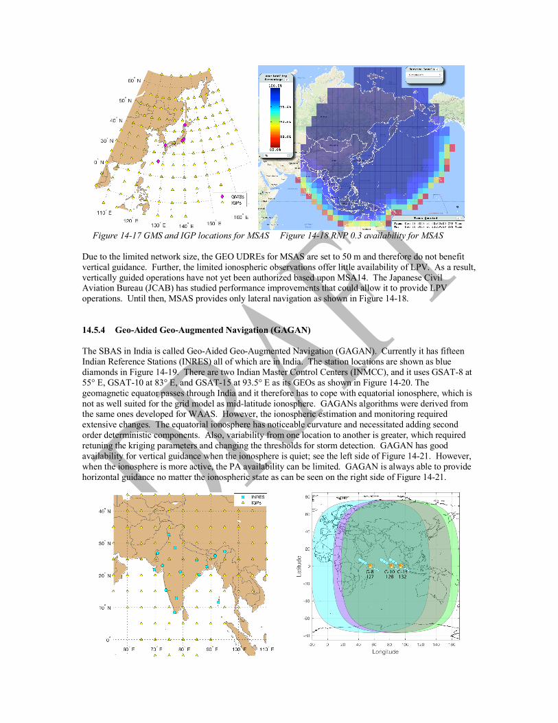
Figure 14-17 GMS and IGP locations for MSAS Figure 14-18 RNP 0.3 availability for MSAS Due to the limited network size, the GEO UDREs for MSAS are set to 50 m and therefore do not benefit vertical guidance. Further, the limited ionospheric observations offer little availability of LPV. As a result, vertically guided operations have not yet been authorized based upon MSA14. The Japanese Civil Aviation Bureau (JCAB) has studied performance improvements that could allow it to provide LPV operations. Until then, MSAS provides only lateral navigation as shown in Figure 14-18. 14.5.4 Geo-Aided Geo-Augmented Navigation (GAGAN) The SBAS in India is called Geo-Aided Geo-Augmented Navigation (GAGAN). Currently it has fifteen Indian Reference Stations (INRES) all of which are in India. The station locations are shown as blue diamonds in Figure 14-19. There are two Indian Master Control Centers (INMCC), and it uses GSAT-8 at 55° E, GSAT-10 at 83° E, and GSAT-15 at 93.5° E as its GEOs as shown in Figure 14-20. The geomagnetic equator passes through India and it therefore has to cope with equatorial ionosphere, which is not as well suited for the grid model as mid-latitude ionosphere. GAGANs algorithms were derived from the same ones developed for WAAS. However, the ionospheric estimation and monitoring required extensive changes. The equatorial ionosphere has noticeable curvature and necessitated adding second order deterministic components. Also, variability from one location to another is greater, which required retuning the kriging parameters and changing the thresholds for storm detection. GAGAN has good availability for vertical guidance when the ionosphere is quiet; see the left side of Figure 14-21. However, when the ionosphere is more active, the PA availability can be limited. GAGAN is always able to provide horizontal guidance no matter the ionospheric state as can be seen on the right side of Figure 14-21.

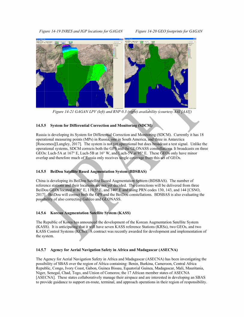
Figure 14-19 INRES and IGP locations for GAGAN Figure 14-20 GEO footprints for GAGAN

Figure 14-21 GAGAN LPV (left) and RNP 0.3 (right) availability (courtesy AAI [AAI])

14.5.5 System for Differential Correction and Monitoring (SDCM) Russia is developing its System for Differential Correction and Monitoring (SDCM). Currently it has 18 operational measuring points (MPs) in Russia, one in South America, and three in Antarctica [Roscomos][Langley, 2017]. The system is not yet operational but does broadcast a test signal. Unlike the operational systems, SDCM corrects both the GPS and the GLONASS constellations. It broadcasts on three GEOs: Luch-5A at 167° E, Luch-5B at 16° W, and Luch-5V at 95° E. These GEOs only have minor overlap and therefore much of Russia only receives single coverage from this set of GEOs. 14.5.5 BeiDou Satellite Based Augmentation System (BDSBAS) China is developing its BeiDou Satellite Based Augmentation System (BDSBAS). The number of reference stations and their locations are not yet decided. The corrections will be delivered from three BeiDou GEOs located at 80° E, 110.5° E, and 140° E and using PRN codes 130, 143, and 144 [CSNO, 2017]. BeiDou will correct both the GPS and the BeiDou constellations. BDSBAS is also evaluating the possibility of also correcting Galileo and GLONASS. 14.5.6 Korean Augmentation Satellite System (KASS) The Republic of Korea has announced the development of the Korean Augmentation Satellite System (KASS). It is anticipating that it will have seven KASS reference Stations (KRSs), two GEOs, and two KASS Control Systems (KCSs). A contract was recently awarded for development and implementation of the system. 14.5.7 Agency for Aerial Navigation Safety in Africa and Madagascar (ASECNA) The Agency for Aerial Navigation Safety in Africa and Madagascar (ASECNA) has been investigating the possibility of SBAS over the region of Africa containing: Benin, Burkina, Cameroon, Central Africa Republic, Congo, Ivory Coast, Gabon, Guinea Bissau, Equatorial Guinea, Madagascar, Mali, Mauritania, Niger, Senegal, Chad, Togo, and Union of Comoros; the 17 African member states of ASECNA [ASECNA]. These states collaboratively manage their airspace and are interested in developing an SBAS to provide guidance to support en-route, terminal, and approach operations in their region of responsibility.

They have conducted tests in coordinating with EGNOS and are investigating adapting the EGNOS algorithms to provide service over Africa [Lapie, 2016]. 14.6 Future Evolutions (Dual Frequency, Multi-Constellation) There are major innovations occurring on the core constellations: GPS is adding new signals including a civil signal at L5, GLONASS is improving the performance of its satellites, and Galileo and BeiDou are filling out the remainder of their planned constellations. SBAS is also planning to evolve along with these improvements. Current SBAS receivers only process GPS L1 C/A signals. The next generation of SBAS receivers will exploit signals on at least two different frequencies and from multiple constellations [Walter, 2011]. The details for exploiting these Dual-Frequency Multi-Constellation (DFMC) enhancements are still in the process of being developed. At the moment, there is significant effort in developing how to incorporate the L5 GPS signals and the E1 and E5A Galileo signals. However, the intention is that this early work will be extended to GLONASS and BeiDou signals as well. The L5 and E5 signals are attractive as they overlap each other and are in a protected Aeronautical Radio Navigation Service (ARNS) frequency band (unlike GPS L2 or Galileo E6 for example). ARNS bands are protected for aviation use and have lower concerns over other transmissions overwhelming these signals. The joint use of L1 with L5 (and E1 with E5a) is especially attractive because the signals can be combined in a manner to cancel the first order ionospheric delay effect. This iono-free combination reduces the ionospherically induced ranging error to a satellite from tens of meters to a few centimeters (usually even lower) [Datta-Barua, 2006]. Thus, the dominant source of uncertainty for the current L1-only SBAS systems can be virtually eliminated for a dual-frequency SBAS. The coverage regions for vertical guidance shown in previous plots could be dramatically expanded. Further, far fewer reference stations are required as there would be no need to estimate and send ionospheric grid corrections. Instead, the user directly estimates and removes the ionospheric delay along each of their lines of sight. The only penalty is that independent individual errors on each frequency become amplified. Thus, the effects of multipath are increased by a factor of 2.26 on L1 and 1.26 on L5 (if the error is equal on each frequency, the overall effect is increased by 2.6) [Walter, 2011]. For L1-only SBAS, the ionospheric correction uncertainty, reflected in the GIVEs, is by far the largest term in (14-1), while the sair term is the smallest. For dual-frequency SBAS, the error term on an individual satellite is given by (14-4) where is the dual-frequency clock and ephemeris bound and is the iono-free user noise and multipath bound. This term is used in place of (14-1) for the dual-frequency SBAS user. The inclusion of additional constellations into SBAS also promises to significantly improve their performance. Having more ranging measurements means that a user is very unlikely to suffer from weak geometry. Further, extra ranging measurements average down the effect of noise and uncertainty. Roughly speaking, doubling the number of ranging measurements will divide the protection level values by approximately the square root of two (about a 30% reduction). The constellations have different signal properties and thus their clocks are not precisely coordinated form one constellation to another. Further, the constellation timing differences may be larger than the dynamic range of the corrections. Therefore, the user needs to add another clock state to be estimated for each additional constellation from which they use ranging measurements. This estimated clock state will absorb both the differences in the constellation time base, and also those due to the different signal structure employed by the new constellation.

σ i,DF

2 = σ DFC ,i

2 +σ tropo,i

2 +σ air _ iono− free,i

2

σ DFC ,i

2 σ air _ iono− free,i

2

Figure 14-22 Existing L1-only LPV coverage Figure 14-23 DF LPV coverage for existing systems Figure 14-22 shows the LPV coverage provided by the currently operating systems. As can be seen, coverage is limited to the four regions: North America, Europe, Japan, and India. Figure 14-23 shows the coverage if those four systems all implemented dual frequency. This modeling further assumes that EGNOS switches from using MT27 to using MT28. Dual frequency eliminates the reliance on the ionospheric grid and large associated uncertainty at the edges of each system. Now coverage expands well beyond the original borders. The current systems only provide LPV service to approximately 11% of the Earth’s surface. Switching to dual frequency nearly triples the area covered to now over 31%. Adding another constellation to the set of corrections nearly doubles the area covered to 59%. Figure 14-24 shows this result when these same four systems provide DFMC service correcting both GPS and Galileo. These results are calculated using Stanford University’s Matlab Algorithm Availability Simulation Toolset (MAAST) [Jan, 2001]. MAAST uses the locations of the reference stations and satellites (obtained from the constellation almanacs) and replicates the UDRE and GIVE algorithms for each of the different systems. It is able to then estimate the resulting VPL and HPL at each time step and user location to compute expected availability. MAAST provides the ability to evaluate DFMC algorithms long before any DFMC capable receivers are fielded or satellites are launched. It is used extensively by WAAS to determine which algorithm candidates are most worthy of pursuing. It allows SBAS providers to estimate the expected levels of service for future evolutions as can be seen in Figures 14-23 to 14-25.

Figure 14-24 DFMC LPV coverage for existing systems Figure 14-25 DFMC LPV coverage for all systems Figure 14-25 shows the resulting LPV availability if the remaining planned SBASs are also implemented with DFMC service. The most significant expansion is now over Africa. This is because all of the planned

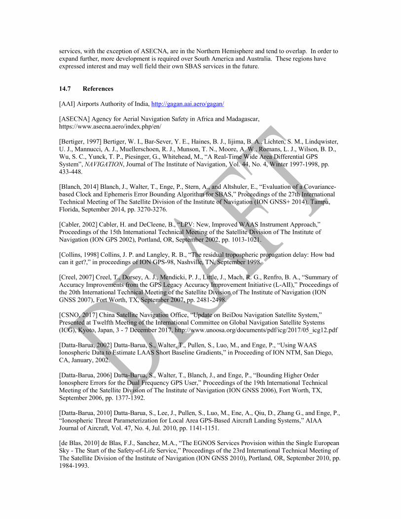
services, with the exception of ASECNA, are in the Northern Hemisphere and tend to overlap. In order to expand further, more development is required over South America and Australia. These regions have expressed interest and may well field their own SBAS services in the future. 14.7 References [AAI] Airports Authority of India, http://gagan.aai.aero/gagan/ [ASECNA] Agency for Aerial Navigation Safety in Africa and Madagascar, https://www.asecna.aero/index.php/en/ [Bertiger, 1997] Bertiger, W. I., Bar-Sever, Y. E., Haines, B. J., Iijima, B. A., Lichten, S. M., Lindqwister, U. J., Mannucci, A. J., Muellerschoen, R. J., Munson, T. N., Moore, A. W., Romans, L. J., Wilson, B. D., Wu, S. C., Yunck, T. P., Piesinger, G., Whitehead, M., “A Real-Time Wide Area Differential GPS System”, NAVIGATION, Journal of The Institute of Navigation, Vol. 44, No. 4, Winter 1997-1998, pp. 433-448. [Blanch, 2014] Blanch, J., Walter, T., Enge, P., Stern, A., and Altshuler, E., “Evaluation of a Covariance-based Clock and Ephemeris Error Bounding Algorithm for SBAS,” Proceedings of the 27th International Technical Meeting of The Satellite Division of the Institute of Navigation (ION GNSS+ 2014), Tampa, Florida, September 2014, pp. 3270-3276. [Cabler, 2002] Cabler, H. and DeCleene, B., “LPV: New, Improved WAAS Instrument Approach,” Proceedings of the 15th International Technical Meeting of the Satellite Division of The Institute of Navigation (ION GPS 2002), Portland, OR, September 2002, pp. 1013-1021. [Collins, 1998] Collins, J. P. and Langley, R. B., “The residual tropospheric propagation delay: How bad can it get?,” in proceedings of ION GPS-98, Nashville, TN, September 1998. [Creel, 2007] Creel, T., Dorsey, A. J., Mendicki, P. J., Little, J., Mach, R. G., Renfro, B. A., “Summary of Accuracy Improvements from the GPS Legacy Accuracy Improvement Initiative (L-AII),” Proceedings of the 20th International Technical Meeting of the Satellite Division of The Institute of Navigation (ION GNSS 2007), Fort Worth, TX, September 2007, pp. 2481-2498. [CSNO, 2017] China Satellite Navigation Office, “Update on BeiDou Navigation Satellite System,” Presented at Twelfth Meeting of the International Committee on Global Navigation Satellite Systems (ICG), Kyoto, Japan, 3 - 7 December 2017, http://www.unoosa.org/documents/pdf/icg/2017/05_icg12.pdf [Datta-Barua, 2002] Datta-Barua, S., Walter, T., Pullen, S., Luo, M., and Enge, P., “Using WAAS Ionospheric Data to Estimate LAAS Short Baseline Gradients,” in Proceeding of ION NTM, San Diego, CA, January, 2002. [Datta-Barua, 2006] Datta-Barua, S., Walter, T., Blanch, J., and Enge, P., “Bounding Higher Order Ionosphere Errors for the Dual Frequency GPS User,” Proceedings of the 19th International Technical Meeting of the Satellite Division of The Institute of Navigation (ION GNSS 2006), Fort Worth, TX, September 2006, pp. 1377-1392. [Datta-Barua, 2010] Datta-Barua, S., Lee, J., Pullen, S., Luo, M., Ene, A., Qiu, D., Zhang G., and Enge, P., “Ionospheric Threat Parameterization for Local Area GPS-Based Aircraft Landing Systems,” AIAA Journal of Aircraft, Vol. 47, No. 4, Jul. 2010, pp. 1141-1151. [de Blas, 2010] de Blas, F.J., Sanchez, M.A., “The EGNOS Services Provision within the Single European Sky - The Start of the Safety-of-Life Service,” Proceedings of the 23rd International Technical Meeting of The Satellite Division of the Institute of Navigation (ION GNSS 2010), Portland, OR, September 2010, pp. 1984-1993.

[DeCleene, 2000] DeCleene, B., “Defining Pseudorange Integrity - Overbounding,” Proceedings of the 13th International Technical Meeting of the Satellite Division of The Institute of Navigation (ION GPS 2000), Salt Lake City, UT, September 2000, pp. 1916-1924. [ESSP] European Satellite Services Provider, https://egnos-user-support.essp-sas.eu/new_egnos_ops/index.php [Ericson 2010] Ericson, S. D., Shallberg, K. W., and Edgar, C. E., “Characterization and Simulation of SVN49 (PRN01) Elevation Dependent Measurement Biases,” Proceedings of the 2010 International Technical Meeting of The Institute of Navigation, San Diego, CA, January 2010, pp. 963-974. [FAATC] William J. Hughes FAA Technical Center, http://www.nstb.tc.faa.gov [Gordon, 2010] Gordon, S., Sherrell, C., Potter, B.J., “WAAS Offline Monitoring,” Proceedings of the 23rd International Technical Meeting of The Satellite Division of the Institute of Navigation (ION GNSS 2010), Portland, OR, September 2010, pp. 2021-2030. [GPS, 2017] GPS “Interface Specification IS-GPS-200,” IRN-IS-200H-005 May 2017 available at: https://www.gps.gov/technical/icwg/ [Gratton, 2007] Gratton, L., Pramanik, R., Tang, H., Pervan, B., “Ephemeris Failure Rate Analysis and its Impact on Category I LAAS Integrity,” Proceedings of the 20th International Technical Meeting of the Satellite Division of The Institute of Navigation (ION GNSS 2007), Fort Worth, TX, September 2007, pp. 386-394. [GSA, 2016] Gobal Navigation satellite Systems Agency, “EGNOS Safety of Life (SoL) Service Definition Document 3.1,” September, 2016 available at: https://egnos-user-support.essp-sas.eu/new_egnos_ops/sites/default/files/library/official_docs/egnos_sol_sdd_in_force.pdf [Gunning, 2017] Gunning, K., Walter, T., and Enge, P., “Characterization of GLONASS Broadcast Clock and Ephemeris: Nominal Performance and Fault Trends for ARAIM,” Presented January 2017 at the Institute of Navigation (ION) International Technical Meeting, Monterey, California. [Haines, 2005] Haines, B., Bar-Sever, Y., Bertiger, W., Byun, S., Desai S., and Hajj, G., “GPS Antenna Phase Center Variations: New Perspectives From the GRACE Mission,” Dynamic Planet 2005, Cairns, Australia. [Hansen, 1998] Hansen, A., Walter, T., Lawrence, D., and Enge, P., “GPS Satellite Clock Event of SV#27 and Its Impact on Augmented Navigation Systems,” in proceedings of ION GPS-98, Nashville, TN, September 1998. [Heng, 2010] Heng, L., Gao, G. X., Walter, T., Enge, P., “GPS Signal-in-Space Anomalies in the Last Decade: Data Mining of 400,000,000 GPS Navigation Messages,” Proceedings of the 23rd International Technical Meeting of The Satellite Division of the Institute of Navigation (ION GNSS 2010), Portland, OR, September 2010, pp. 3115-3122. [Heng, 2011] Heng, L., Gao, G. X., Walter, T., Enge, P., “Statistical Characterization of GPS Signal-In-Space Errors,” Proceedings of the 2011 International Technical Meeting of The Institute of Navigation, San Diego, CA, January 2011, pp. 312-319. [Heng , 2012] Heng, L., Gao, G. X., Walter, T., and Enge, P., “GLONASS Signal-in-Space Anomalies Since 2009,” Proceedings of the 25th International Technical Meeting of The Satellite Division of the Institute of Navigation (ION GNSS 2012), Nashville, TN, September 2012, pp. 833-842.

[Holland, 1973] Holland, F. , Rucker R. , and Horowitz, B., “Structure of the Airspace,” in IEEE Transactions on Communications, vol. 21, no. 5, pp. 382-398, May 1973. doi: 10.1109/TCOM.1973.1091698 [Hsu, 2008] Hsu, P. H., Chiu, T., Golubev, Y., and Phelts, R.E. “Test Results for the WAAS Signal Quality Monitor,” Proceedings of IEEE/ION PLANS 2008, Monterey, CA, May 2008, pp. 263-270. [ICAO, 2006] International Civil Aviation Organization (ICAO), “International Standards and Recommended Practices, Annex 10 to the Convention on International Civil Aviation, Volume I Radio Navigation Aids,” 6th Edition, July 2006. [Jan, 2001] Jan, S. S., Chan, W., Walter, T., and Enge, P., “Matlab Simulation Toolset for SBAS Availability Analysis,” Proceedings of the 14th International Technical Meeting of the Satellite Division of The Institute of Navigation (ION GPS 2001), Salt Lake City, UT, September 2001, pp. 2366-2375. [Jefferson, 2000] Jefferson, D. C. and Bar-Sever, Y. E., “Accuracy and Consistency of GPS Broadcast Ephemeris Data,” in Proceeding of ION GPS-2000, Salt Lake City, UT, September 2000. [Komjathy, 2002] Komjathy, A., Wilson, B.D., Runge, T.F., Boulat, B.M., Mannucci, A.J., Sparks, L., Reyes, M.J., “A New Ionospheric Model for Wide Area Differential GPS: The Multiple Shell Approach,” Proceedings of the 2002 National Technical Meeting of The Institute of Navigation, San Diego, CA, January 2002, pp. 460-466. [Komjathy, 2004] Komjathy, A., Sparks, L., Mannucci, A. J., and Coster, A., “The Ionospheric Impact of the October 2003 Storm Event on WAAS,” Proceedings of the 17th International Technical Meeting of the Satellite Division of The Institute of Navigation (ION GNSS 2004), Long Beach, CA, September 2004, pp. 1298-1307. [Langley, 2017] Langley, R. B., “Innovation: GLONASS — past, present and future,” GPS World November 1, 2017, http://gpsworld.com/innovation-glonass-past-present-and-future/ [Lapie, 2016] Lapie, J., “SBAS-ASECNA Programme Update” Presented at the EGNOS Service Provision Workshop in Warsaw, Poland on 27-28 September 2016, available at: https://egnos-user-support.essp-sas.eu/new_egnos_ops/sites/default/files/workshop2016/08.%20ASECNA%20-%20SBAS-ASECNA%20Programme%20Update.pdf [Lawrence, 2007] Lawrence, D., Bunce, D., Mathur, N. G., Sigler, C. E., “Wide Area Augmentation System (WAAS) - Program Status,” Proceedings of the 20th International Technical Meeting of the Satellite Division of The Institute of Navigation (ION GNSS 2007), Fort Worth, TX, September 2007, pp. 892-899. [Montenbruck, 2010] Montenbruck, O., Hauschild, A., Steigenberger, P., and Langley, R. B., “Three’s the Challenge,” GPS World, July, 2010 [Paredes, 2008] Paredes, E., Pandya, N., Sparks, L., and Komjathy, A., “Reconstructing the WAAS Undersampled Ionospheric Gradient Threat Model for the WAAS Expansion into Mexico,” Proceedings of the 21st International Technical Meeting of the Satellite Division of The Institute of Navigation (ION GNSS 2008), Savannah, GA, September 2008, pp. 1938-1947. [Phelts 2003] Phelts, R. E., Walter, T., Enge, P., “Toward Real- Time SQM for WAAS: Improved Detection Techniques,” Proceedings of the 16th International Technical Meeting of the Satellite Division of the Institute of Navigation, ION GPS/GNSS-2003, September 2003. [Phelts, 2009] Phelts, R.E., Walter, T., Enge, P., “Characterizing Nominal Analog Signal Deformation on GNSS Signals,” Proceedings of the 22nd International Technical Meeting of The Satellite Division of the Institute of Navigation (ION GNSS 2009), Savannah, GA, September 2009, pp. 1343-1350.

[Phelts, 2015] Phelts, R. E., Altshuler, E., Walter, T., and Enge, P., “Validating Nominal Bias Error Limits Using 4 years of WAAS Signal Quality Monitoring Data,” Proceedings of the ION 2015 Pacific PNT Meeting, Honolulu, Hawaii, April 2015, pp. 956-963. [Rajagopal, 2004] Rajagopal, S., Walter, T., Datta-Barua, S., Blanch, J., and Sakai, T., “Correlation Structure of the Equatorial Ionosphere,” Proceedings of the 2004 National Technical Meeting of The Institute of Navigation, San Diego, CA, January 2004, pp. 542-550. [Rivers, 2000] Rivers, M. H., “2 SOPS Anomaly Resolution on an Aging Constellation,” Proceedings of the 13th International Technical Meeting of the Satellite Division of The Institute of Navigation (ION GPS 2000), Salt Lake City, UT, September 2000, pp. 2547-2550. [Roscomos] http://www.sdcm.ru/index_eng.html [RTCA, 2016] RTCA, DO-229E, “Minimum Operational Performance Standards for Global Positioning System/Satellite-Based Augmentation System Airborne Equipment (SBAS MOPS),” prepared by RTCA SC-159, December, 2016. [Sakai, 2013] Sakai, T. and Tashiro, H., “MSAS Status,” Proceedings of the 26th International Technical Meeting of The Satellite Division of the Institute of Navigation (ION GNSS+ 2013), Nashville, TN, September 2013, pp. 2343-2360. [Senior, 2008] Senior, Kenneth L., Ray, Jim R., Beard, Ronald L. “Characterization of periodic variations in the GPS satellite clocks,” GPS Solutions, Vol, 12, Issue 3, pp 211–225, July 2008, doi 10.1007/s10291-008-0089-9 [Shallberg, 2001] Shallberg, K., Shloss, P., Altshuler, E., and Tahmazyan, L., “WAAS Measurement Processing, Reducing the Effects of Multipath,” in Proceeding of ION GPS-2001, Salt Lake City, UT, September 2001. [Shallberg, 2002] Shallberg, K. and Grabowski, J., “Considerations for Characterizing Antenna Induced Range Errors,” Proceedings of the 15th International Technical Meeting of the Satellite Division of The Institute of Navigation (ION GPS 2002), Portland, OR, September 2002, pp. 809-815. [Shallberg, 2008] Shallberg, K. and Sheng, F., “WAAS Measurement Processing; Current Design and Potential Improvements,” Proceedings of IEEE/ION PLANS 2008, Monterey, CA, May 2008, pp. 253-262. [Shallberg, 2017] Shallberg, K. W., Ericson, S. D., Phelts, E., Walter, T., Kovach, K., and Altshuler, E., “Catalog and Description of GPS and WAAS L1 C/A Signal Deformation Events,” Proceedings of the 2017 International Technical Meeting of The Institute of Navigation, Monterey, California, January 2017, pp. 508-520. [Shank, 1993] Shank, C. M. and Lavrakas, J. “GPS Integrity: An MCS Perspective,” in Proceeding of ION GPS-1993, Salt Lake City, UT, September 1993. [Shloss, 2002] Shloss, P., Phelts, R. E., Walter, T., Enge, P., “A Simple Method of Signal Quality Monitoring for WAAS LNAV/VNAV,” Proceedings of the 15th International Technical Meeting of the Satellite Division of The Institute of Navigation (ION GPS 2002), Portland, OR, September 2002, pp. 800-808. [SIWG, 2003] SBAS Ionospheric Working Group, “Ionospheric Research Issues for SBAS – A White Paper,” February 2003, available at: http://web.stanford.edu/group/scpnt/gpslab/website_files/sbas-ion_wg/sbas_iono_white_feb2003.pdf

[Sparks, 2005] Sparks, L., A. Komjathy, A.J. Mannucci, E. Altshuler, T. Walter, J. Blanch, M. Bakry El- Arini, and R. Lejeune, “Extreme Ionospheric Storms and Their Impact on WAAS,” Proceedings of the Ionospheric Effects Symposium 2005, Alexandria VA, 2005. [Sparks, 2011a] Sparks, L., J. Blanch, and N. Pandya, “Estimating ionospheric delay using kriging: 1. Methodology,” Radio Sci., 46, 2011, doi:10.1029/2011RS004667. [Sparks, 2011b] Sparks, L., J. Blanch, and N. Pandya, “Estimating ionospheric delay using kriging: 2. Impact on satellite-based augmentation system availability,” Radio Sci., 46, 2011, doi:10.1029/2011RS004781. [Sparks , 2014] Sparks, L. and Altshuler, E., “Improving WAAS Availability Along the Coast of California,” Proceedings of the 27th International Technical Meeting of The Satellite Division of the Institute of Navigation (ION GNSS+ 2014), Tampa, Florida, September 2014, pp. 3299-3311. [Walter, 1997] Walter, T., Enge, P., and Hansen, A., “A Proposed Integrity Equation for WAAS MOPS,” Proceedings of the 10th International Technical Meeting of the Satellite Division of The Institute of Navigation (ION GPS 1997), Kansas City, MO, September 1997, pp. 475-484. [Walter, 1999] Walter, T., “WAAS MOPS: Practical Examples,” Proceedings of the 1999 National Technical Meeting of The Institute of Navigation, San Diego, CA, January 1999, pp. 283-293. [Walter, 2001a]Walter, T., Hansen, A., and Enge, P., “Message Type 28,” Proceedings of the 2001 National Technical Meeting of The Institute of Navigation, Long Beach, CA, January 2001, pp. 522-532. [Walter, 2001b] Walter, T., et al. “Robust Detection of Ionospheric Irregularities,” in NAVIGATION, Journal of the Institute of Navigation, vol. 48, no. 2, Summer 2001. [Walter, 2003] Walter, T., Enge, P., and DeCleene, B., “Integrity Lessons from the WAAS Integrity Performance Panel (WIPP),” Proceedings of the 2003 National Technical Meeting of The Institute of Navigation, Anaheim, CA, January 2003, pp. 183-194. [Walter, 2004] Walter, T., Rajagopal, S., Datta-Barua, S., and Blanch, J. A, “Protecting Against Unsampled Ionospheric Threats,” Presented October 2004 at the Beacon Satellite Symposium, Trieste, Italy. [Walter, 2011] Walter, T., Blanch, J., Phelts, R. E., and Enge, P, “Evolving WAAS to Serve L1/L5 Users,” Proceedings of the 24th International Technical Meeting of The Satellite Division of the Institute of Navigation (ION GNSS 2011), Portland, OR, September 2011, pp. 2495-2504. [Walter, 2012] Walter, Todd, Blanch, Juan, Phelts, R. Eric, Enge, Per, "Evolving WAAS to Serve L1/L5 Users", NAVIGATION, Journal of The Institute of Navigation, Vol. 59, No. 4, Winter 2012, pp. 317-327. [Walter, 2015] Walter, T. and Blanch, J., “Characterization of GNSS Clock and Ephemeris Errors to Support ARAIM,” Proceedings of the ION 2015 Pacific PNT Meeting, Honolulu, Hawaii, April 2015, pp. 920-931. [Walter, 2016] Walter, T., Blanch, J., Joerger, M., and Pervan, B., “Determination of Fault Probabilities for ARAIM,” Proceedings of IEEE/ION PLANS 2016, Savannah, GA, April 2016, pp. 451-461. [Walter, 2017a] Walter, T. and Blanch, J., “Improved User Position Monitor for WAAS,” Published in NAVIGATION, Vol. 64, No. 1, Spring 2017, pp. 165-175, DOI 10.1002/navi.180. [Walter, 2017b] Walter, T., Gunning, K., Phelts, R. E., and Blanch, J., “Validation of the Unfaulted Error Bounds for ARAIM.” Presented May 2017 at the Institute of Navigation (ION) Positioning, Navigation and Timing Conference, Honolulu, Hawaii.

[Walter, 2018] Walter, T., Shallberg, K., Altshuler, e., Wanner, W., Harris, C., and Stimmler, R., “WAAS at 15,” Proceedings of the 2018 International Technical Meeting of The Institute of Navigation, Reston, VA, January 2018. [WGC, 2013] E.U. U.S. Bilateral Working Group C, “Interim Report of ARAIM Technical Subgroup,” available at https://www.gps.gov/policy/cooperation/europe/2013/working-group-c/ [Wong, 2011] Wong, G., Phelts, R.E., Walter, T., and Enge, P., “Bounding Errors Caused by Nominal GNSS Signal Deformations,” Proceedings of the 24th International Technical Meeting of The Satellite Division of the Institute of Navigation (ION GNSS 2011), Portland, OR, September 2011. [Wu, 2002] Wu, T., Peck, Stephen, “An Analysis of Satellite Integrity Monitoring Improvement for WAAS,” Proceedings of the 15th International Technical Meeting of the Satellite Division of The Institute of Navigation (ION GPS 2002), Portland, OR, September 2002, pp. 756-765.