Chapter 12 The Keynesian Model and the Phillips Curve · The Keynesian Model and the Phillips Curve...

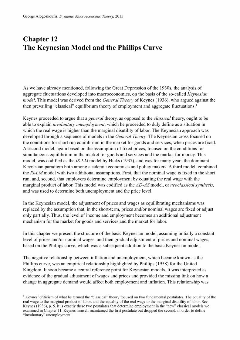
George Alogoskoufis, Dynamic Macroeconomic Theory, 2015

Chapter 12 The Keynesian Model and the Phillips Curve

As we have already mentioned, following the Great Depression of the 1930s, the analysis of aggregate fluctuations developed into macroeconomics, on the basis of the so-called Keynesian model. This model was derived from the General Theory of Keynes (1936), who argued against the then prevailing “classical” equilibrium theory of employment and aggregate fluctuations. 1

Keynes proceeded to argue that a general theory, as opposed to the classical theory, ought to be able to explain involuntary unemployment, which he proceeded to duly define as a situation in which the real wage is higher than the marginal disutility of labor. The Keynesian approach was developed through a sequence of models in the General Theory. The Keynesian cross focused on the conditions for short run equilibrium in the market for goods and services, when prices are fixed. A second model, again based on the assumption of fixed prices, focused on the conditions for simultaneous equilibrium in the market for goods and services and the market for money. This model, was codified as the IS-LM model by Hicks (1937), and was for many years the dominant Keynesian paradigm both among academic economists and policy makers. A third model, combined the IS-LM model with two additional assumptions. First, that the nominal wage is fixed in the short run, and, second, that employers determine employment by equating the real wage with the marginal product of labor. This model was codified as the AD-AS model, or neoclassical synthesis, and was used to determine both unemployment and the price level.

In the Keynesian model, the adjustment of prices and wages as equilibrating mechanisms was replaced by the assumption that, in the short-term, prices and/or nominal wages are fixed or adjust only partially. Thus, the level of income and employment becomes an additional adjustment mechanism for the market for goods and services and the market for labor.

In this chapter we present the structure of the basic Keynesian model, assuming initially a constant level of prices and/or nominal wages, and then gradual adjustment of prices and nominal wages, based on the Phillips curve, which was a subsequent addition to the basic Keynesian model.

The negative relationship between inflation and unemployment, which became known as the Phillips curve, was an empirical relationship highlighted by Phillips (1958) for the United Kingdom. It soon became a central reference point for Keynesian models. It was interpreted as evidence of the gradual adjustment of wages and prices and provided the missing link on how a change in aggregate demand would affect both employment and inflation. This relationship was

Keynes’ criticism of what he termed the “classical” theory focused on two fundamental postulates. The equality of the 1

real wage to the marginal product of labor, and the equality of the real wage to the marginal disutility of labor. See Keynes (1936), p. 5. It is exactly these two postulates that determine employment in the “new” classical models we examined in Chapter 11. Keynes himself maintained the first postulate but dropped the second, in order to define “involuntary” unemployment.

George Alogoskoufis, Dynamic Macroeconomic Theory, 2015 Chapter 12

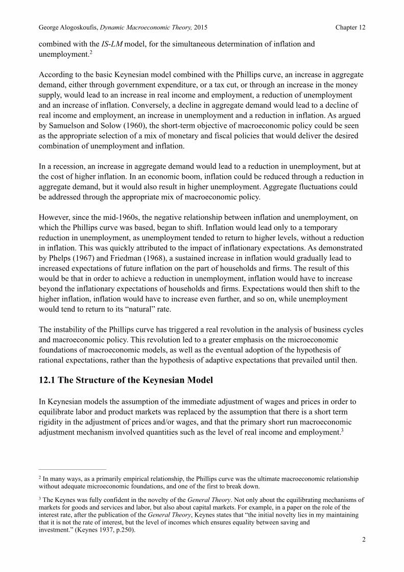
combined with the IS-LM model, for the simultaneous determination of inflation and unemployment. 2

According to the basic Keynesian model combined with the Phillips curve, an increase in aggregate demand, either through government expenditure, or a tax cut, or through an increase in the money supply, would lead to an increase in real income and employment, a reduction of unemployment and an increase of inflation. Conversely, a decline in aggregate demand would lead to a decline of real income and employment, an increase in unemployment and a reduction in inflation. As argued by Samuelson and Solow (1960), the short-term objective of macroeconomic policy could be seen as the appropriate selection of a mix of monetary and fiscal policies that would deliver the desired combination of unemployment and inflation.

In a recession, an increase in aggregate demand would lead to a reduction in unemployment, but at the cost of higher inflation. In an economic boom, inflation could be reduced through a reduction in aggregate demand, but it would also result in higher unemployment. Aggregate fluctuations could be addressed through the appropriate mix of macroeconomic policy.

However, since the mid-1960s, the negative relationship between inflation and unemployment, on which the Phillips curve was based, began to shift. Inflation would lead only to a temporary reduction in unemployment, as unemployment tended to return to higher levels, without a reduction in inflation. This was quickly attributed to the impact of inflationary expectations. As demonstrated by Phelps (1967) and Friedman (1968), a sustained increase in inflation would gradually lead to increased expectations of future inflation on the part of households and firms. The result of this would be that in order to achieve a reduction in unemployment, inflation would have to increase beyond the inflationary expectations of households and firms. Expectations would then shift to the higher inflation, inflation would have to increase even further, and so on, while unemployment would tend to return to its “natural” rate.

The instability of the Phillips curve has triggered a real revolution in the analysis of business cycles and macroeconomic policy. This revolution led to a greater emphasis on the microeconomic foundations of macroeconomic models, as well as the eventual adoption of the hypothesis of rational expectations, rather than the hypothesis of adaptive expectations that prevailed until then.

12.1 The Structure of the Keynesian Model

In Keynesian models the assumption of the immediate adjustment of wages and prices in order to equilibrate labor and product markets was replaced by the assumption that there is a short term rigidity in the adjustment of prices and/or wages, and that the primary short run macroeconomic adjustment mechanism involved quantities such as the level of real income and employment. 3

In many ways, as a primarily empirical relationship, the Phillips curve was the ultimate macroeconomic relationship 2

without adequate microeconomic foundations, and one of the first to break down.

The Keynes was fully confident in the novelty of the General Theory. Not only about the equilibrating mechanisms of 3

markets for goods and services and labor, but also about capital markets. For example, in a paper on the role of the interest rate, after the publication of the General Theory, Keynes states that “the initial novelty lies in my maintaining that it is not the rate of interest, but the level of incomes which ensures equality between saving and investment.” (Keynes 1937, p.250).

!2


In this section we shall look at the three main forms of traditional Keynesian model. First, we shall examine the Keynesian cross, which determines real output and employment as a function of real aggregate demand. Second, the IS-LM model, which determines real output and employment and the nominal interest rate as a function of real aggregate demand and monetary conditions. Thirdly we shall introduce the AD-AS model of aggregate demand and aggregate supply, that determines real income and the price level, for given nominal wages. All three forms can be found in successive chapters of the General Theory which develop the Keynesian model.

12.1.1 The Keynesian Cross

The Keynesian model starts by considering the determination of aggregate demand. The assumption is that total real output and income Y, is equal to the sum of real consumption C, real gross investment Ι and real government expenditure G.

(12.1)

In the simplest version, that of the Keynesian cross, investment and government expenditure are considered exogenous, and consumption is assumed to be a positive function of current real disposable income.

, (12.2)

where T denotes taxes, and CY is the marginal propensity to consume. Thus, (12.2) is the Keynesian consumption function.

From (12.1) and (12.2) we get the equilibrium condition between total output and aggregate demand, which is the equilibrium condition in the market for goods and services.

(12.3)

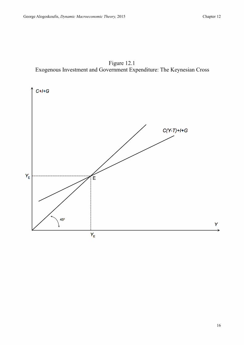
The equilibrium condition (12.3) is depicted in Figure 12.1, which is also known as the Keynesian cross.

Real output is determined by the equality of aggregate supply and aggregate demand, which is the sum of real consumption, investment and government expenditure. Prices are assumed fixed or sluggish to adjust, so a change in aggregate demand brings about a change in aggregate supply through corresponding changes in employment. 4

From equation (12.3), one can derive the multiplier.

(12.4)

Yt = Ct + It +Gt

Ct = C Yt −Tt( ) 0 <CY =∂C

∂(Y −T )<1

Yt = C Yt −Tt( ) + It +Gt

dYtdIt

= dYtdGt

= 11−CY

>1

The assumption here is that output is at less than full employment, and that an increase in aggregate demand causes 4

firms to increase labor demand, employment and output. Implicitly, because of involuntary unemployment, labor supply is assumed perfectly elastic.

!3


An exogenous change in aggregate demand, either through investment or through government expenditure, results in a change in real output which is a multiple of the original change which is higher than one, since the marginal propensity to consume is less than one. When aggregate demand increases, real output and income increases in order to maintain equilibrium between real output and expenditure. This causes an induced increase in private consumption through the consumption function, which brings about a further increase in real output and income. Consequently, a given exogenous rise in aggregate demand has a multiple effect on aggregate real income, due to the second round effects through aggregate consumption, which in turn produce further increases in real demand and real output and employment. 5

From equation (12.3) one can also derive the balanced budget multiplier, that is the effects of a change in government expenditure and taxes that leaves the budget deficit unchanged. Under the assumption that dGt=dTt, it follows that,

(12.5)

An increase in public expenditure, funded by an equal increase in taxes, increases total aggregate expenditure and real output and income by the same amount. This is something that was proven by Haavelmo (1945). Government expenditure increases aggregate demand one to one, but the tax increase reduces private consumption by less than one to one, because the marginal propensity to consume is less than one. Consequently, the initial impact on overall expenditure is 1-CY, and the overall effect of a change in government expenditure financed by increased taxes is equal to unity.

The model of the Keynesian cross, assumes that investment is exogenous. In an important paper, Samuelson (1939) combined this model with an investment function based on the principle of acceleration, to derive endogenous business cycles in the Keynesian model. The analysis of the Samuelson multiplier-accelerator model, one of the first Keynesian models of endogenous fluctuations, is presented in the Annex to this chapter. 6

12.1.2 The IS-LM Model

A more general form of the basic Keynesian model considers that aggregate investment depends on the real interest rate, and introduces the equilibrium condition in the market for money, in order to analyze the simultaneous determination of real output and the interest rate. This form was codified as the IS-LM model, in the important contribution of Hicks (1937), and is the best known version of the Keynesian model. 7

dYtdGt dGt=dTt

= 1

The explanation of aggregate consumption function and the multiplier take up Chapters 8 to 10 in Keynes (1936), and 5

constitute the important analytical chapters for the General Theory.

The principle of acceleration, as a basis for a theory of investment, has a long history in the analysis of business 6

cycles. It assumes that investment is a positive function of the change in total output or the change in consumption. Aftalion (1909), Bickerdike (1914) and Clark (1917) were early analyses of business cycles based on this principle. See Knox (1952) for a survey.

This form of the model, which is a generalization of the Keynesian cross, is analyzed in Chapters 10 to 18 of Keynes 7

(1936).!4


The main difference from the previous model of the Keynesian cross is that investment ceases to be treated as exogenous, and is considered to depend negatively on the real interest rate. Assuming that inflationary expectations are given, investment will depend negatively on the current nominal interest rate. Consequently, the equilibrium condition in the goods and services market takes the form, 8

(12.6)

where i is the nominal interest rate. The effects of the nominal interest rate on investment are assumed to be negative. Thus,

!

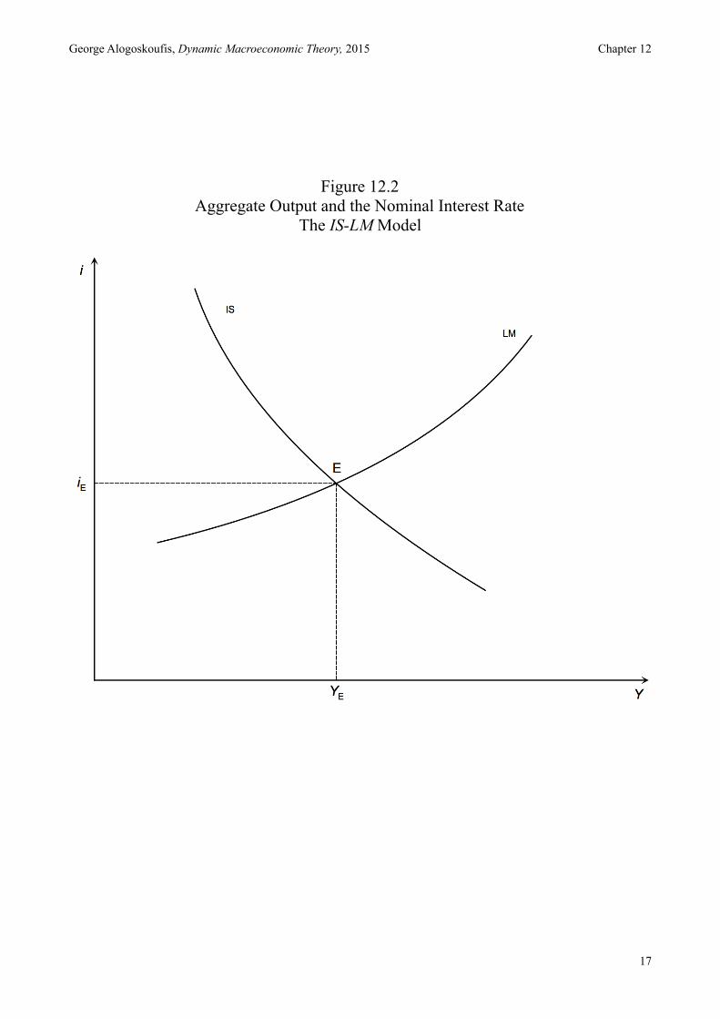
(12.6) describes the combinations of real output and the nominal interest rate that ensure equilibrium in the market for goods and services. It is depicted as the downward sloping IS (Investment-Savings) curve in Figure 12.2.

From the moment a new endogenous variable (the nominal interest rate) is introduced, one should analyze how it is determined. This is done through introducing the equilibrium condition in the money market, i.e. the condition that the demand for money, which is a positive function of aggregate output and a negative function of the nominal interest rate, is equal to the money supply, as defined by the policy of the central bank. The equilibrium condition takes the form,

(12.7)

where Μ is the nominal money supply, P the price level (which is considered as given in this version of the model) and m the demand function for real money balances (liquidity preference). The properties of the money demand function are described by,

!

(12.7) describes the combinations of real output and the nominal interest rate that ensure equilibrium in the money market, in the sense that money demand is equal to the exogenous money supply. It is depicted as the upward sloping LM (Liquidity-Money) curve in Figure 12.2.

Real output and the nominal interest rate are determined at the point where both the market for goods and services and the market for money are in equilibrium. At the point of intersection of the IS curve, which describes equilibrium in the market for goods and services, and the LM curve, which describes equilibrium in the money market, the economy is thus in short run equilibrium. Since the price level is assumed to be fixed, this equilibrium could be at less than full employment. In fact, this is assumption usually made in Keynesian models.

Yt = C Yt −Tt( ) + It (it )+Gt

∂I∂i

< 0

Mt

Pt= m Yt ,it( )

∂m∂Y

> 0, ∂m∂i

< 0

Keynes was fully aware of Fisher’s distinction between the nominal and the real interest rate, as is evident in the 8

discussion in pages 140-143 of the General Theory. However, the implicit assumption in his analysis was that inflationary expectations are given. This was after all consistent with the assumption of short-run price rigidity.

!5


It is simple to deduce that an increase in government expenditure, or a tax cut, shifts the IS curve to the right, and causes an increase in real output and the nominal interest rate. It is also simple to deduce that an increase in the money supply shifts the LM curve to the right, and causes an increase in real income and a reduction in the nominal interest rate. Both fiscal and monetary policies can thus lead to an increase in aggregate demand, and an increase in real output and employment. This is the rationale for aggregate demand policies in the Keynesian model.

12.1.3 The Aggregate Demand (AD), Aggregate Supply (AS) Model

The last and more sophisticated form of the basic Keynesian model is analyzed after Chapter 19 of the General Theory. In this form of the model, the price level ceases to be exogenous, and is allowed to change in order to equilibrate aggregate demand for goods and services with a less than perfectly elastic aggregate supply. However, nominal wages are still considered to be fixed in the short run.

The aggregate demand function (AD) is derived from the simultaneous satisfaction of the equilibrium condition in the market for goods and services (IS) and the equilibrium condition in the money market (LM). From (12.6) and (12.7), substituting for the nominal interest rate, we get an aggregate demand function of the form,

(12.8)

where,

!

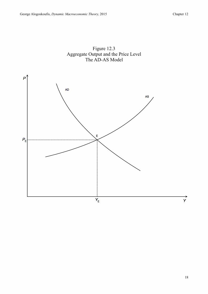
(12.8) describes aggregate demand as a negative function of the price level. A higher price level, given the money supply, means lower real money balances, higher nominal interest rates and lower investment demand. Thus, given the money supply, an increase in the price level reduces aggregate demand, and a fall in the price level, increases aggregate demand. The aggregate demand function is the negatively sloped AD curve in Figure 12.3.

In order to derive the aggregate supply function (AS), we examine the behavior of the representative firm. We assume that the representative firm is competitive and maximizes profits, selecting the level of employment and output, taking nominal wages and prices as given. Output and employment are determined by solving the following problem.

(12.9)

under the constraint,

(12.10)

Yt = DMt

Pt,Gt ,Tt

⎛⎝⎜

⎞⎠⎟

∂D∂Pt

< 0

max PtYt −WtLt[ ]

Yt = F Lt( )

!6


where F is a concave short run production function, depending only on the level of employment L.

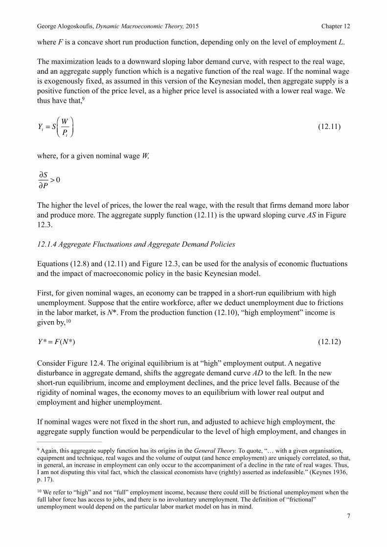
The maximization leads to a downward sloping labor demand curve, with respect to the real wage, and an aggregate supply function which is a negative function of the real wage. If the nominal wage is exogenously fixed, as assumed in this version of the Keynesian model, then aggregate supply is a positive function of the price level, as a higher price level is associated with a lower real wage. We thus have that, 9

(12.11)

where, for a given nominal wage W,

#

The higher the level of prices, the lower the real wage, with the result that firms demand more labor and produce more. The aggregate supply function (12.11) is the upward sloping curve AS in Figure 12.3.

12.1.4 Aggregate Fluctuations and Aggregate Demand Policies

Equations (12.8) and (12.11) and Figure 12.3, can be used for the analysis of economic fluctuations and the impact of macroeconomic policy in the basic Keynesian model.

First, for given nominal wages, an economy can be trapped in a short-run equilibrium with high unemployment. Suppose that the entire workforce, after we deduct unemployment due to frictions in the labor market, is N*. From the production function (12.10), “high employment” income is given by, 10

! (12.12)

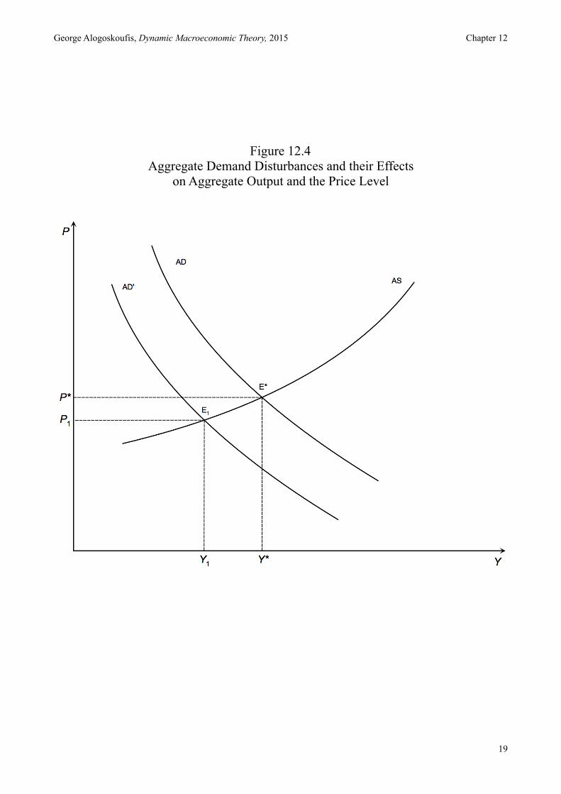
Consider Figure 12.4. The original equilibrium is at “high” employment output. A negative disturbance in aggregate demand, shifts the aggregate demand curve AD to the left. In the new short-run equilibrium, income and employment declines, and the price level falls. Because of the rigidity of nominal wages, the economy moves to an equilibrium with lower real output and employment and higher unemployment.

If nominal wages were not fixed in the short run, and adjusted to achieve high employment, the aggregate supply function would be perpendicular to the level of high employment, and changes in

Yt = SWPt

⎛⎝⎜

⎞⎠⎟

∂S∂P

> 0

Y*= F(N*)

Again, this aggregate supply function has its origins in the General Theory. To quote, “… with a given organisation, 9

equipment and technique, real wages and the volume of output (and hence employment) are uniquely correlated, so that, in general, an increase in employment can only occur to the accompaniment of a decline in the rate of real wages. Thus, I am not disputing this vital fact, which the classical economists have (rightly) asserted as indefeasible.” (Keynes 1936, p. 17).

We refer to “high” and not “full” employment income, because there could still be frictional unemployment when the 10

full labor force has access to jobs, and there is no involuntary unemployment. The definition of “frictional” unemployment would depend on the particular labor market model on has in mind.

!7


aggregate demand would only result in increases in the price level. Consequently, with full flexibility of wages and prices and wages, this model has the same properties as a “classical” model.

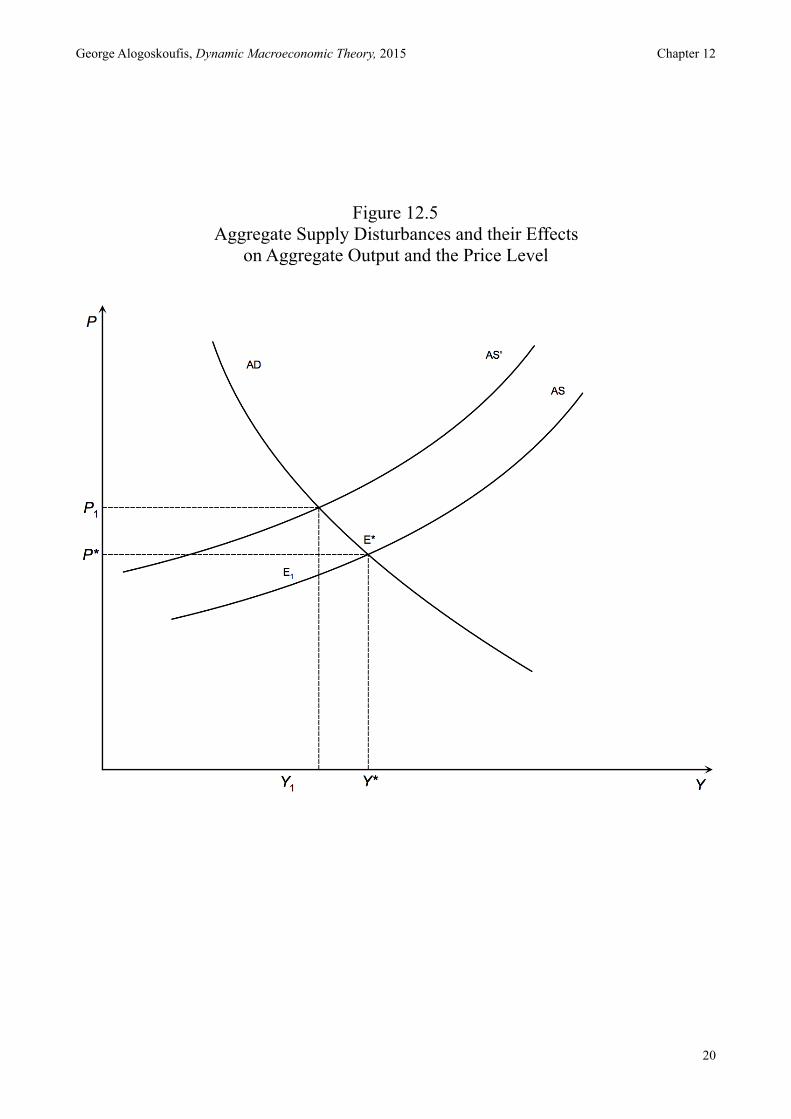
This model can also be used to address the effects of disturbances to aggregate supply. Consider Figure 12.5. The original equilibrium is at “high” employment output. A negative disturbance in aggregate supply, such as negative productivity shock, shifts the aggregate supply curve AS to the left. In the new short-run equilibrium, income and employment declines, and the price level rises. Because of the rigidity of nominal wages, the economy moves to an equilibrium with lower real output and employment and higher unemployment.

In contrast to the “classical” model of full adjustment of wages and prices, in the Keynesian model with nominal wage rigidity, even monetary disturbances can shift aggregate demand and cause fluctuations in real output, employment and other real variables such as real wages and interest rates.

How can the impact of shocks to aggregate demand and supply be addressed? According to the Keynesian approach, an appropriate solution can come from macroeconomic policy. An increase of government expenditure, a reduction in taxes or an increase in the money supply can move the aggregate demand curve to the right, and counteract the consequences of an initial demand or supply shock on real output and unemployment. In the case of demand shocks, the price level returns to its original equilibrium. In the case of a negative supply shock there are further effects on the price level.

This is the justification and the effects of aggregate demand policies in the Keynesian model. In principle, aggregate demand policies, such as monetary policy, could be used to counteract the effects of both demand and supply shocks on aggregate output and unemployment. This would imply that aggregate demand policies could in principle be used to stabilize economies around levels of high employment and help avoid the repetition of phenomena such as the Great Depression.

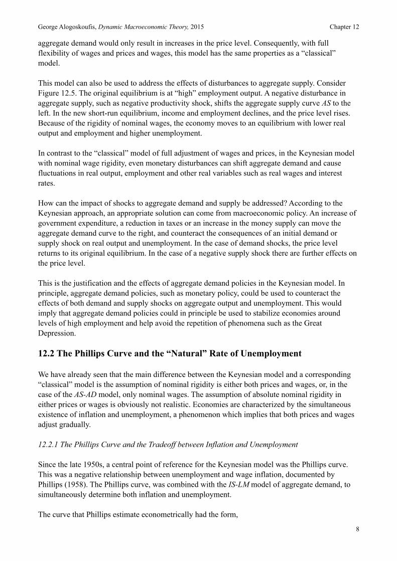
12.2 The Phillips Curve and the “Natural” Rate of Unemployment

We have already seen that the main difference between the Keynesian model and a corresponding “classical” model is the assumption of nominal rigidity is either both prices and wages, or, in the case of the AS-AD model, only nominal wages. The assumption of absolute nominal rigidity in either prices or wages is obviously not realistic. Economies are characterized by the simultaneous existence of inflation and unemployment, a phenomenon which implies that both prices and wages adjust gradually.

12.2.1 The Phillips Curve and the Tradeoff between Inflation and Unemployment

Since the late 1950s, a central point of reference for the Keynesian model was the Phillips curve. This was a negative relationship between unemployment and wage inflation, documented by Phillips (1958). The Phillips curve, was combined with the IS-LM model of aggregate demand, to simultaneously determine both inflation and unemployment.

The curve that Phillips estimate econometrically had the form,

!8


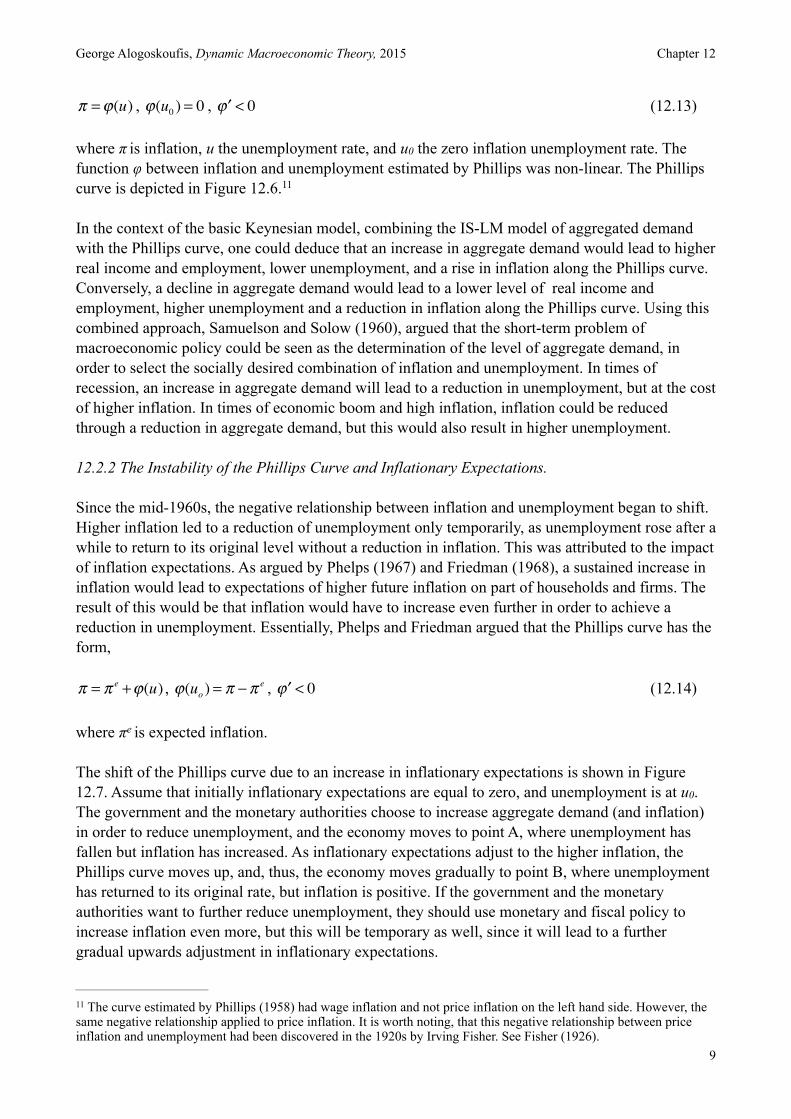
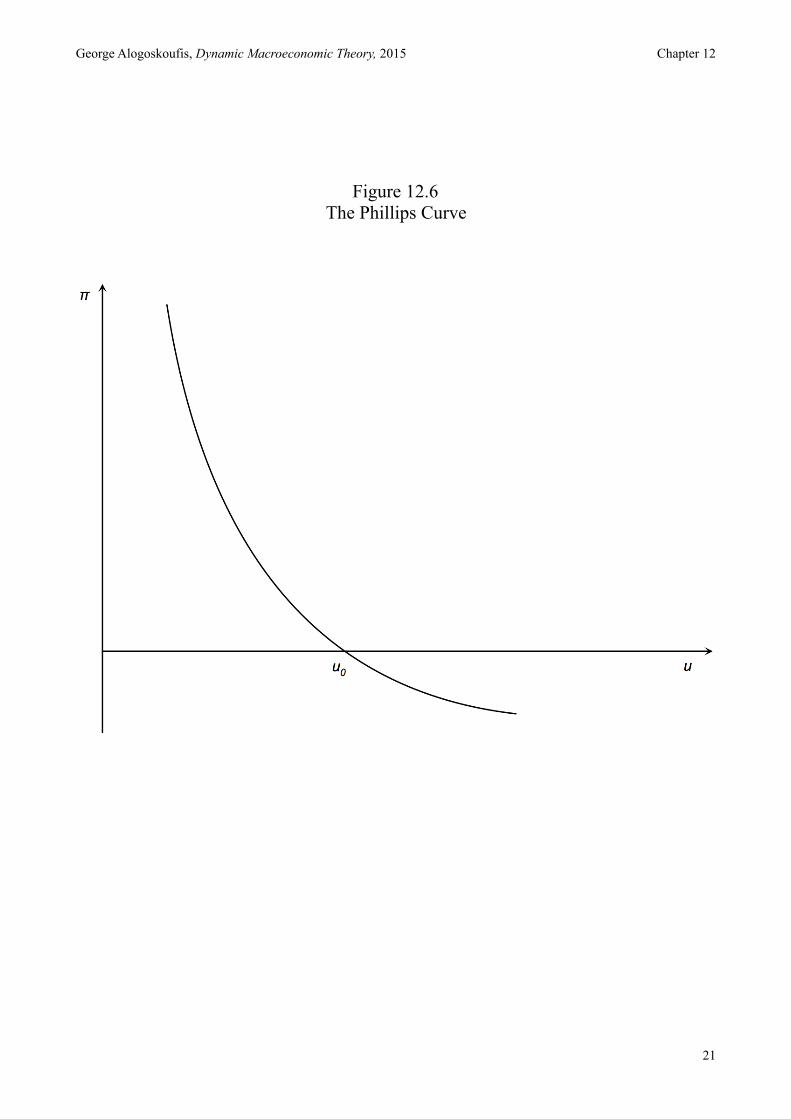
! , ! , ! (12.13)

where π is inflation, u the unemployment rate, and u0 the zero inflation unemployment rate. The function φ between inflation and unemployment estimated by Phillips was non-linear. The Phillips curve is depicted in Figure 12.6. 11

In the context of the basic Keynesian model, combining the IS-LM model of aggregated demand with the Phillips curve, one could deduce that an increase in aggregate demand would lead to higher real income and employment, lower unemployment, and a rise in inflation along the Phillips curve. Conversely, a decline in aggregate demand would lead to a lower level of real income and employment, higher unemployment and a reduction in inflation along the Phillips curve. Using this combined approach, Samuelson and Solow (1960), argued that the short-term problem of macroeconomic policy could be seen as the determination of the level of aggregate demand, in order to select the socially desired combination of inflation and unemployment. In times of recession, an increase in aggregate demand will lead to a reduction in unemployment, but at the cost of higher inflation. In times of economic boom and high inflation, inflation could be reduced through a reduction in aggregate demand, but this would also result in higher unemployment.

12.2.2 The Instability of the Phillips Curve and Inflationary Expectations.

Since the mid-1960s, the negative relationship between inflation and unemployment began to shift. Higher inflation led to a reduction of unemployment only temporarily, as unemployment rose after a while to return to its original level without a reduction in inflation. This was attributed to the impact of inflation expectations. As argued by Phelps (1967) and Friedman (1968), a sustained increase in inflation would lead to expectations of higher future inflation on part of households and firms. The result of this would be that inflation would have to increase even further in order to achieve a reduction in unemployment. Essentially, Phelps and Friedman argued that the Phillips curve has the form,

! , ! , ! (12.14)

where πe is expected inflation.

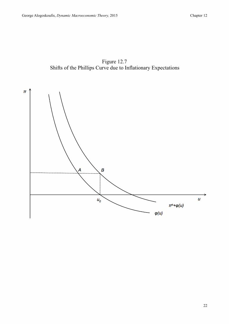
The shift of the Phillips curve due to an increase in inflationary expectations is shown in Figure 12.7. Assume that initially inflationary expectations are equal to zero, and unemployment is at u0. The government and the monetary authorities choose to increase aggregate demand (and inflation) in order to reduce unemployment, and the economy moves to point A, where unemployment has fallen but inflation has increased. As inflationary expectations adjust to the higher inflation, the Phillips curve moves up, and, thus, the economy moves gradually to point B, where unemployment has returned to its original rate, but inflation is positive. If the government and the monetary authorities want to further reduce unemployment, they should use monetary and fiscal policy to increase inflation even more, but this will be temporary as well, since it will lead to a further gradual upwards adjustment in inflationary expectations.

π =ϕ(u) ϕ(u0 ) = 0 ′ϕ < 0

π = π e +ϕ(u) ϕ(uo ) = π −π e ′ϕ < 0

The curve estimated by Phillips (1958) had wage inflation and not price inflation on the left hand side. However, the 11

same negative relationship applied to price inflation. It is worth noting, that this negative relationship between price inflation and unemployment had been discovered in the 1920s by Irving Fisher. See Fisher (1926).

!9


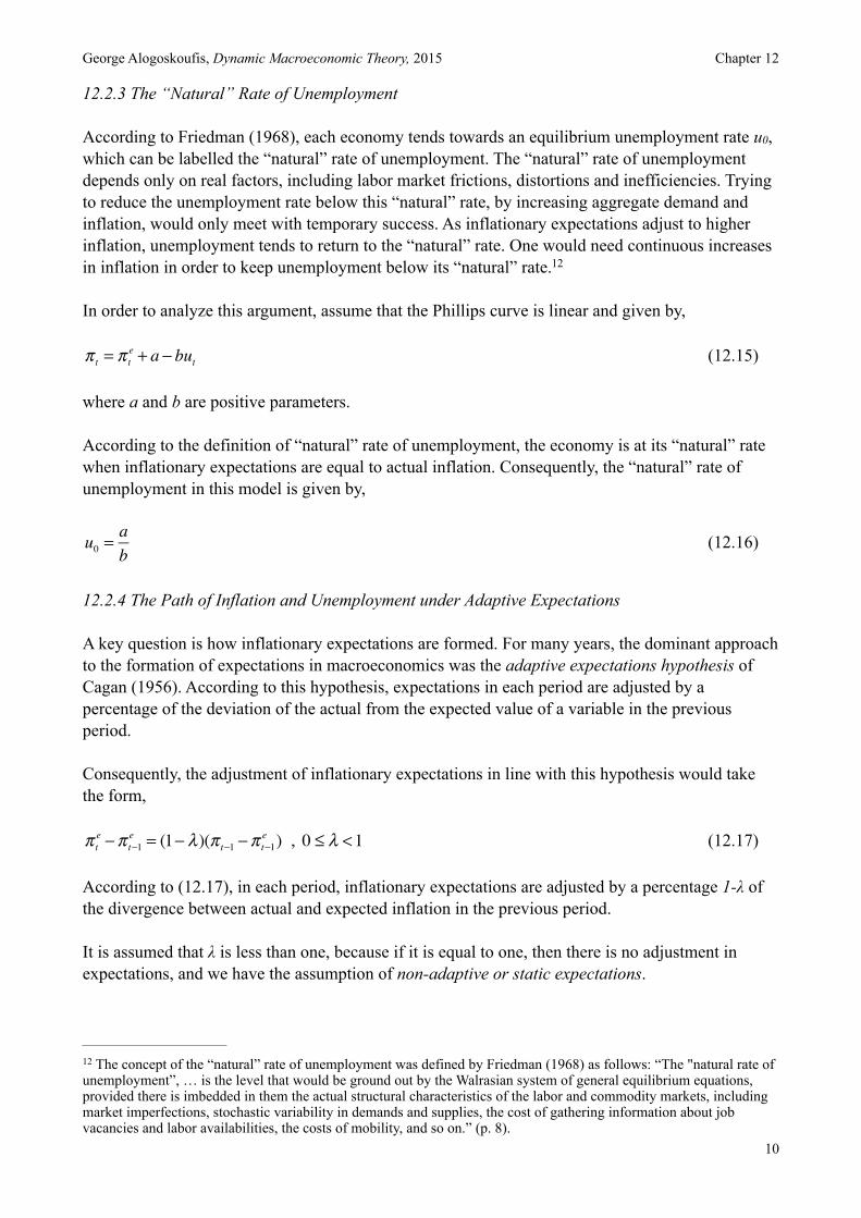
12.2.3 The “Natural” Rate of Unemployment

According to Friedman (1968), each economy tends towards an equilibrium unemployment rate u0, which can be labelled the “natural” rate of unemployment. The “natural” rate of unemployment depends only on real factors, including labor market frictions, distortions and inefficiencies. Trying to reduce the unemployment rate below this “natural” rate, by increasing aggregate demand and inflation, would only meet with temporary success. As inflationary expectations adjust to higher inflation, unemployment tends to return to the “natural” rate. One would need continuous increases in inflation in order to keep unemployment below its “natural” rate. 12

In order to analyze this argument, assume that the Phillips curve is linear and given by,

! (12.15)

where a and b are positive parameters.

According to the definition of “natural” rate of unemployment, the economy is at its “natural” rate when inflationary expectations are equal to actual inflation. Consequently, the “natural” rate of unemployment in this model is given by,

! (12.16)

12.2.4 The Path of Inflation and Unemployment under Adaptive Expectations

A key question is how inflationary expectations are formed. For many years, the dominant approach to the formation of expectations in macroeconomics was the adaptive expectations hypothesis of Cagan (1956). According to this hypothesis, expectations in each period are adjusted by a percentage of the deviation of the actual from the expected value of a variable in the previous period.

Consequently, the adjustment of inflationary expectations in line with this hypothesis would take the form,

! , ! (12.17)

According to (12.17), in each period, inflationary expectations are adjusted by a percentage 1-λ of the divergence between actual and expected inflation in the previous period.

It is assumed that λ is less than one, because if it is equal to one, then there is no adjustment in expectations, and we have the assumption of non-adaptive or static expectations.

π t = π te + a − but

u0 =ab

π te −π t−1

e = (1− λ)(π t−1 −π t−1e ) 0 ≤ λ <1

The concept of the “natural” rate of unemployment was defined by Friedman (1968) as follows: “The "natural rate of 12

unemployment”, … is the level that would be ground out by the Walrasian system of general equilibrium equations, provided there is imbedded in them the actual structural characteristics of the labor and commodity markets, including market imperfections, stochastic variability in demands and supplies, the cost of gathering information about job vacancies and labor availabilities, the costs of mobility, and so on.” (p. 8).

!10


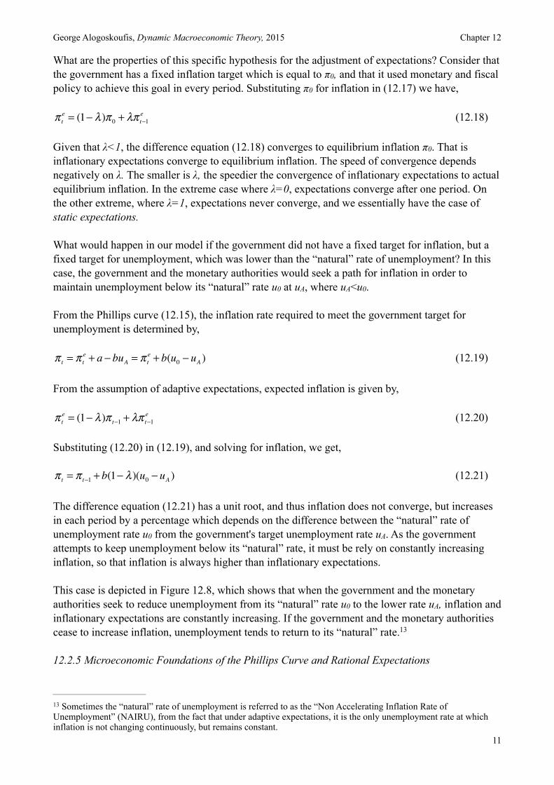
What are the properties of this specific hypothesis for the adjustment of expectations? Consider that the government has a fixed inflation target which is equal to π0, and that it used monetary and fiscal policy to achieve this goal in every period. Substituting π0 for inflation in (12.17) we have,

! (12.18)

Given that λ<1, the difference equation (12.18) converges to equilibrium inflation π0. That is inflationary expectations converge to equilibrium inflation. The speed of convergence depends negatively on λ. The smaller is λ, the speedier the convergence of inflationary expectations to actual equilibrium inflation. In the extreme case where λ=0, expectations converge after one period. On the other extreme, where λ=1, expectations never converge, and we essentially have the case of static expectations.

What would happen in our model if the government did not have a fixed target for inflation, but a fixed target for unemployment, which was lower than the “natural” rate of unemployment? In this case, the government and the monetary authorities would seek a path for inflation in order to maintain unemployment below its “natural” rate u0 at uA, where uA<u0.

From the Phillips curve (12.15), the inflation rate required to meet the government target for unemployment is determined by,

! (12.19)

From the assumption of adaptive expectations, expected inflation is given by,

! (12.20)

Substituting (12.20) in (12.19), and solving for inflation, we get,

! (12.21)

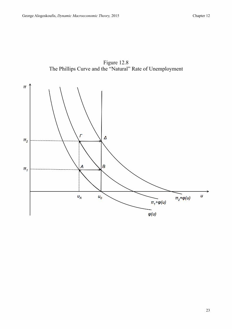
The difference equation (12.21) has a unit root, and thus inflation does not converge, but increases in each period by a percentage which depends on the difference between the “natural” rate of unemployment rate u0 from the government's target unemployment rate uΑ. As the government attempts to keep unemployment below its “natural” rate, it must be rely on constantly increasing inflation, so that inflation is always higher than inflationary expectations.

This case is depicted in Figure 12.8, which shows that when the government and the monetary authorities seek to reduce unemployment from its “natural” rate u0 to the lower rate uA, inflation and inflationary expectations are constantly increasing. If the government and the monetary authorities cease to increase inflation, unemployment tends to return to its “natural” rate. 13

12.2.5 Microeconomic Foundations of the Phillips Curve and Rational Expectations

π te = (1− λ)π 0 + λπ t−1

e

π t = π te + a − buA = π t

e + b(u0 − uA )

π te = (1− λ)π t−1 + λπ t−1

e

π t = π t−1 + b(1− λ)(u0 − uA )

Sometimes the “natural” rate of unemployment is referred to as the “Non Accelerating Inflation Rate of 13

Unemployment” (NAIRU), from the fact that under adaptive expectations, it is the only unemployment rate at which inflation is not changing continuously, but remains constant.

!11


The instability of the original Phillips curve observed in the late 1960s, and the interpretation given to it by Phelps and Friedman, sparked a revolution in the analysis of aggregate fluctuations and macroeconomic policy.

The literature has since moved in two directions.

First, great emphasis was placed on the microeconomic foundations of the determination of wages, prices, the supply and demand for goods and services and the determination of the equilibrium unemployment rate. The result is that today both “new classical” and the “new Keynesian” models of aggregate fluctuations are based on dynamic stochastic general equilibrium models with detailed and consistent microeconomic foundations. 14

Secondly, this development led to the adoption of the hypothesis of rational expectations, namely the hypothesis that households and firms form inflationary expectations taking into account the motives of governments and monetary authorities to choose between inflation and unemployment. The hypothesis of rational expectations is currently the key hypothesis regarding the formation of expectations, non only about inflation, but all future variables that affect the behavior of households and firms, as well as governments. 15

Both of these developments will be analyzed in the chapters that follow.

12.3 Conclusions

In this chapter we have introduced the basic Keynesian model, which was associated with the development of macroeconomics from the mid-1930s to the end of the 1960s.

We have shown that what separates classical from Keynesian models is the assumption of nominal rigidity and/or gradual adjustment in nominal wages and the price level.

Much of the theoretical research of the last five decades has focused on the microeconomic foundations of the Keynesian model, and in particular the Phillips curve. This is an important part of the so-called new Keynesian approach. In the next chapter we analyze a simple dynamic model that belongs to this category and look at the predictions of the “new” Keynesian approach for aggregate fluctuations and the relationship between inflation and unemployment.

See Phelps E.S. (1970) for a collection of models which started off this research program. The new classical model of 14

aggregate fluctuations (Ch.11), the new Keynesian approach to aggregate fluctuations (Ch. 13-14) and the matching model of equilibrium unemployment (Ch. 15) are all based on this important collection of models of 1970.

See Lucas (1972), who introduced the hypothesis of rational expectations of Muth (1961) to modern 15

macroeconomics.!12


Annex to Chapter 12: The Samuelson Multiplier-Accelerator Model

In an important paper, Samuelson (1939) combined the model of the Keynesian cross with an investment function based on the principle of acceleration, to derive endogenous cycles. Samuelson considered the following version of the Keynesian model.

! (A12.1)

! (A12.2)

! (A.12.3)

! (A.12.4)

a,b,c,d and e are constant parameters. a is the accelerator, which determines how a change in consumption affects current investment, and b is autonomous investment. c<1 is the marginal propensity to consume, and d is autonomous consumption. Finally e is government expenditure, assumed constant.

The investment function (A12.2) is based on the so called acceleration principle, which implies that when there is a positive change in consumption, firms will invest more, in order to produce the higher quantity of consumer goods demanded. When there is a negative change in consumption, firms will reduce investment, as they need less capital to meet the lower demand for consumer goods. The accelerator a measures the sensitivity of investment to changes in aggregate consumption.

(A.12.3) is a linear Keynesian consumption function, according to which consumption is a function of lagged and not current income.

Government expenditure is assumed exogenous and constant at e.

Substituting (A12.2) in (A.12.2), the investment function can be written as,

! (A.12.5)

Investment is a function of the lagged change in income, as the lagged change in income drives the demand for consumption goods.

Substituting the consumption function (A.12.3), the investment function (A.12.5), and (A.12.4) in the equilibrium condition of the market for goods and services (A.12.1), and collecting terms, one gets,

! (A.12.6)

The path of output is thus determined by the second order difference equation (A.12.6).

The particular solution of this equation, which defines equilibrium output, is given by,

Yt = Ct + It +Gt

It = a(Ct −Ct−1)+ b

Ct = cYt−1 + d

Gt = e

It = ac(Yt−1 −Yt−2 )+ b

Yt = c(1+ a)Yt−1 − acYt−2 + b + d + e

!13


! (A.12.7)

Equilibrium output depends only on autonomous expenditure and the multiplier 1/(1-c), as suggested by the model of the Keynesian cross. However, the path of output is determined by the difference equation (A.12.6), which also depends on the accelerator. 16

For the difference equation (A.12.6) to be stable, ac must be less than one, or the accelerator must satisfy a<1/c. If this condition is not satisfied, output will diverge.

For the roots to be real, the condition is that, c ≥ 4a/(1+a)2. Thus, for the roots to be real and for income to converge monotonically to its equilibrium value, the condition is,

! (A.12.8)

For (A.12.8) to be satisfied, if the marginal propensity to consume is equal to three quarters (0.75), the accelerator must be less than or equal to one third (0.333). In such a case the difference equation will converge monotonically.

If the accelerator is such that the inequality on left hand side of (A.12.8) is strict, the roots will be real and distinct, and less than one. The general solution of (A.12.6) will take the form,

! (A.12.9)

where Y1, Y2 are two boundary (initial conditions) and, λ1, λ2 <1 , the two real and distinct roots of the difference equation, which satisfy,

! , !

Real output will converge monotonically to its equilibrium level Y*, given in (A.12.7).

If the left hand side of (A.12.8) is equal to c, then we shall have two repeated roots, λ= c(1+a)/2<1. The general solution of (A.12.6) will take the form,

! (A.12.10)

Real output will converge monotonically to its equilibrium level Y*, given in (A.12.7).

In the case where the inequality on the left hand side of (A.12.8) is not satisfied, then we shall have two complex roots λ1, λ2, and real output will display oscillations, i.e endogenous fluctuations, during the convergence to its equilibrium value. This will occur as long as a<1/c. If the accelerator does not satisfy this condition, then the model displays divergent oscillations.

Y*= b + d + e1− c

4a(1+ a)2

≤ c < 1a

Yt =b + d + e1− c

+Y1λ1t +Y2λ2

t

λ1 + λ2 = c(1+ a) λ1λ2 = ca <1

Yt =b + d + e1− c

+Y1λt +Y2tλ

t

For the solution of second order linear difference equations see Mathematical Annex 2.16

!14


The complex roots will take the form of a pair of complex conjugates of the form,

! , !

where, ! and ! .

The general solution will then take the form,

! (A.12.11)

where θ is defined by,

! , ! .

This solution will display oscillations of a periodic nature. Since we have assumed that ac<1, the oscillations will be dampened, and there will be cyclical convergence to the equilibrium value given by (A.12.7).

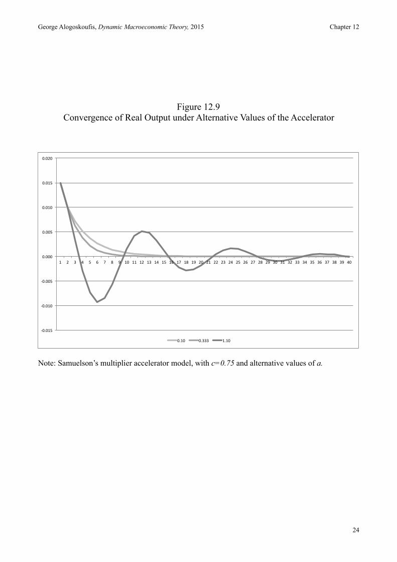
In Figure 12.9 we present the dynamic convergence of real output, for different values of the accelerator, assuming that the equilibrium value is equal to zero.

We assume that c=0.75, and that the accelerator takes three alternative values. 1. a=1/10, 2. a=1/3, and 3. a=11/10. Case 1 results in two real and distinct rules, and monotonic convergence to equilibrium, Case 2 results in repeated real roots and monotonic convergence to equilibrium, and Case 3 results in complex roots and cyclical convergence to equilibrium. Thus, if the accelerator is sufficiently high in this model, there will be cyclical convergence.

λ1 = µ +νi λ2 = µ −νi

µ = c(1+ a)2

ν = 4ac − c2 (1+ a)2

2

Yt =b + d + e1− c

+ ac( )t (Y1 +Y2 )cos(θt)+ (Y1 −Y2 )sin(θt)( )

cos(θ ) = µac

sin(θ ) = νac

!15


Figure 12.1 Exogenous Investment and Government Expenditure: The Keynesian Cross

!

!16


Figure 12.2 Aggregate Output and the Nominal Interest Rate

The IS-LM Model

!

!17


Figure 12.3 Aggregate Output and the Price Level

The AD-AS Model

!

!18


Figure 12.4 Aggregate Demand Disturbances and their Effects

on Aggregate Output and the Price Level

!

!19


Figure 12.5 Aggregate Supply Disturbances and their Effects

on Aggregate Output and the Price Level

!20


Figure 12.6 The Phillips Curve

!21


Figure 12.7 Shifts of the Phillips Curve due to Inflationary Expectations

!22


Figure 12.8 The Phillips Curve and the “Natural” Rate of Unemployment

!23


Figure 12.9 Convergence of Real Output under Alternative Values of the Accelerator

Note: Samuelson’s multiplier accelerator model, with c=0.75 and alternative values of a.

!24

!0.015&

!0.010&

!0.005&

0.000&

0.005&

0.010&

0.015&

0.020&

1& 2& 3& 4& 5& 6& 7& 8& 9& 10& 11& 12& 13& 14& 15& 16& 17& 18& 19& 20& 21& 22& 23& 24& 25& 26& 27& 28& 29& 30& 31& 32& 33& 34& 35& 36& 37& 38& 39& 40&

0.10& 0.333& 1.10&


References

Aftalion A. (1909), “La réalité des surproductions générales”, Revue d’Economie Politique, 22, pp. 219-220.

Bickerdike C.F. (1914), “A Non-Monetary Cause of Fluctuations in Employment”, The Economic Journal, 24, pp. 357-370.

Clark J.M. (1917), “Business Acceleration and the Law of Demand: A Technical Factor in Economic Cycles”, Journal of Political Economy, 25, pp. 217-235.

Fisher I. (1926), “A Statistical Relation between Unemployment and Price Changes”, International Labour Review, 13, pp. 785-92.

Friedman M. (1968), “The Role of Monetary Policy”, American Economic Review, 58, pp. 1-17. Haavelmo T. (1945), “Multiplier Effects of a Balanced Budget”, Econometrica, 13, pp. 311-318. Hicks J.R. (1937), “Mr Keynes and the Classics: A Suggested Interpretation”, Econometrica, 5, pp.

147-159. Keynes J.M. (1936), The General Theory of Employment, Interest and Money, Macmillan, London. Keynes J.M. (1937), “Alternative Theories of the Rate of Interest”, The Economic Journal, 47, pp.

241-252. Knox A.D. (1952), “The Acceleration Principle and the Theory of Investment: A Survey”,

Economica, 19, pp. 269-297. Lucas R.E. Jr (1972), “Expectations and the Neutrality of Money”, Journal of Economic Theory, 4,

pp. 103-124. Muth J.F. (1961), “Rational Expectations and the Theory of Price Movements”, Econometrica, 29,

pp. 315-335. Phelps E.S. (1967), “Phillips Curves, Expectations of Inflation and Optimal Unemployment over

Time”, Economica, 34, pp. 254-281. Phelps E.S. (1970), “Introduction” in Phelps E.S. et al, Microeconomic Foundations of Employment

and Inflation Theory, New York, W.W. Norton. Phillips A.W. (1958), “The Relationship between Unemployment and the Rate of Change of Money

Wages in the United Kingdom, 1861-1957”, Economica, 25, pp. 283-299. Samuelson P.A. (1939), “Interactions between the Multiplier Analysis and the Principle of

Acceleration”, Review of Economics and Statistics, 21, pp. 75-78. Samuelson P.A. and Solow R.M. (1960), “Analytical Aspects of Anti-Inflation Policy”, American

Economic Review, 50, pp. 177-194.

!25

Chapter 12 The Keynesian Model and the Phillips Curve · The Keynesian Model and the Phillips Curve...

Documents

Transcript of Chapter 12 The Keynesian Model and the Phillips Curve · The Keynesian Model and the Phillips Curve...