Chapter 12 Money, Banking, Prices, and Monetary Policy Copyright © 2014 Pearson Education, Inc.
44
Chapter 12 Money, Banking, Prices, and Monetary Policy Copyright © 2014 Pearson Education, Inc.
-
Upload
christal-elliott -
Category
Documents
-
view
219 -
download
1
Transcript of Chapter 12 Money, Banking, Prices, and Monetary Policy Copyright © 2014 Pearson Education, Inc.

Chapter 12
Money, Banking,
Prices, and Monetary
Policy
Copyright © 2014 Pearson Education, Inc.

1-2© 2014 Pearson Education, Inc.
Chapter 12 Topics
• What is money?
• Monetary Intertemporal Model
• Real and nominal interest rates.
• Demand for money – banks and alternative means of payment.
• Neutrality of money
• Short-run non-neutrality of money
• Zero lower bound and quantitative easing.

1-3© 2014 Pearson Education, Inc.
What is Money?
• Medium of exchange
• Store of value
• Unit of account

1-4© 2014 Pearson Education, Inc.
Measures of Money
• Monetary Base (outside money) = currency in circulation + bank reserves.
• M1 = currency in circulation + transactions deposits + travelers’ checks + demand deposits.
• M2 = M1 + savings deposits + retail money market funds.

1-5© 2014 Pearson Education, Inc.
Monetary Aggregates, June 2012 (in $billions)

1-6© 2014 Pearson Education, Inc.
The Inflation Rate
P
PPi
'

1-7© 2014 Pearson Education, Inc.
The Fisher Relation
i
Rr
1
11

1-8© 2014 Pearson Education, Inc.
The Approximate Fisher Relation
iRr

1-9© 2014 Pearson Education, Inc.
Figure 12.1Real and Nominal Interest Rates

1-10© 2014 Pearson Education, Inc.
Banks and Alternative Means of Payment
• Assume all goods must be purchased with currency or credit cards.
• “Credit cards” can be assumed to stand in, more broadly, for debt cards and checks, for example – all alternative means of payment supplied by the financial system.
• Goods purchased at price P, no matter what means of payment is used.

1-11© 2014 Pearson Education, Inc.
Banks and Alternative Means of Payment
• Using a credit card costs q per unit of goods purchased.
• Credit supply (by banks) is given by Xs(q), which is increasing in q.
• Supplying credit card services is costly for banks.

1-12© 2014 Pearson Education, Inc.
Figure 12.2The Supply Curve for Credit Card Services

1-13© 2014 Pearson Education, Inc.
Demand for Credit Card Services
• Quantity of goods purchased with credit card services:
• Goods purchased with currency:
• If
then all goods are purchased with credit cards.
• If
then all goods are purchased with currency.
( )dX q
( )dY X q
(1 ) (1 ),P R P q
(1 ) (1 ),P R P q

1-14© 2014 Pearson Education, Inc.
Figure 12.3Equilibrium in the Market for Credit Card Services

Figure 12.4The Effect of an Increase in the Nominal Interest Rate on the Market for Credit Card Services
1-15© 2014 Pearson Education, Inc.

1-16© 2014 Pearson Education, Inc.
Demand for Money
*[ ( )]dM P Y X R
• Here, X*(R) is the equilibrium quantity of credit card services (decreasing function of R). Therefore, more simply,
),( RYPLM d

1-17© 2014 Pearson Education, Inc.
Demand for Money
• Increasing in real income – more currency required as volume of transactions increases.
• Decreasing in the nominal interest rate. The nominal interest rate is the opportunity cost of using currency in transactions – higher R implies greater use of credit in
transactions, and less use of currency.

1-18© 2014 Pearson Education, Inc.
Nominal Money Demand
• Substitute using the approximate Fisher relation.
• For our experiments, suppose inflation rate is zero (harmless).
),( irYPLM d
),( rYPLM d

1-19© 2014 Pearson Education, Inc.
Figure 12.5The Nominal Money Demand Curve in the Monetary Intertemporal Model

1-20© 2014 Pearson Education, Inc.
The Firm’s Labor Demand
• As in Chapter 4, the firm’s labor demand schedule is the marginal product of labor for the firm, which is downward sloping.

1-21© 2014 Pearson Education, Inc.
Figure 12.6The Effect of an Increase in Current Real Income on the Nominal Money Demand Curve

1-22© 2014 Pearson Education, Inc.
Figure 12.7The Current Money Market in the Monetary Intertemporal Model

1-23© 2014 Pearson Education, Inc.
Figure 12.8The Complete Monetary Intertemporal Model

1-24© 2014 Pearson Education, Inc.
Figure 12.9A Level Increase in the Money Supply in the Current Period

1-25© 2014 Pearson Education, Inc.
The Neutrality of Money
• In the monetary intertemporal model, a level increase in the money supply increases the price level and the nominal wage in proportion to the money supply increase, but has no effect on any real macroeconomic variable.

1-26© 2014 Pearson Education, Inc.
Figure 12.10The Effects of a Level Increase in M—The Neutrality of Money

1-27© 2014 Pearson Education, Inc.
Shifts in Money Demand
• These shifts are important for how monetary policy should be conducted.
• Shifts in the demand for money that occur within a day, week or month (the very short run) are a critical for the central bank.

1-28© 2014 Pearson Education, Inc.
Figure 12.11A Shift in the Supply of Credit Card Services

1-29© 2014 Pearson Education, Inc.
Figure 12.12A Shift in the Demand for Money

Figure 12.13Instability in Money Demand
1-30© 2014 Pearson Education, Inc.

1-31© 2014 Pearson Education, Inc.
Sources of Shifts in the Demand for Money
• Shocks that the central bank is concerned with (in our model): shifts in money demand, output demand, output supply.
• Two alternative policy rules which central banks have adopted: money supply targeting, interest rate targeting.
• Key problem for the central bank: it cannot observe the shocks directly, and does not have timely information on all economic variables.

1-32© 2014 Pearson Education, Inc.
The Short-Run Nonneutrality of Money: Friedman-Lucas Money Surprise Model
• Imperfect information: consumers know the market nominal wage, but they do not observe all prices simultaneously, so they do not know their real wage.
• Different aggregate shocks hit the economy – money supply shocks and productivity shocks – and consumers cannot observe these shocks directly.
• When a worker sees an increase in the nominal wage, what happened to prices?

1-33© 2014 Pearson Education, Inc.
An Increase in the Money Supply in the Friedman-Lucas Money Surprise Model
• Money supply increases – unanticipated and unobserved by the private sector.
• Workers see an increase in their nominal wage, and think that their real wage has increased.
• Workers supply more labor, and output increases.• Nonneutrality of money, but only because people are
fooled into working harder.
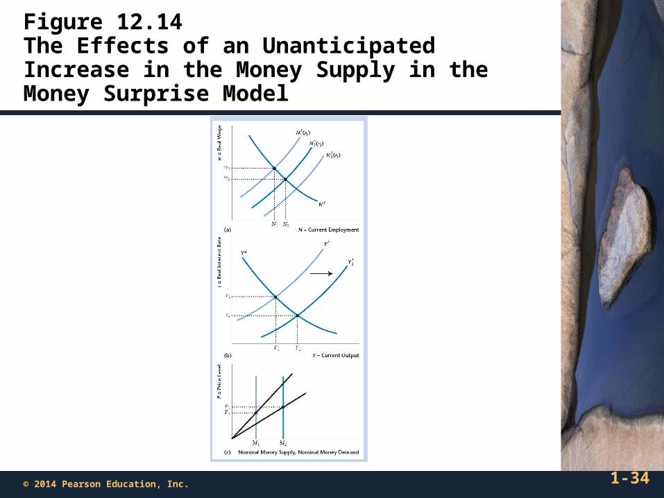
1-34© 2014 Pearson Education, Inc.
Figure 12.14The Effects of an Unanticipated Increase in the Money Supply in the Money Surprise Model

1-35© 2014 Pearson Education, Inc.
Money Supply Targeting and Interest Rate Targeting
• Basic money surprise model seems to indicate that predictability of the money supply is good policy.
• In the model, this means a constant M. In practice it means targeting the growth rate in the quantity of money.
• This works well for productivity shocks, but not for money demand shocks.
• For money demand shocks, interest rate targeting works well.

1-36© 2014 Pearson Education, Inc.
Figure 12.15A Surprise Increase in Money Demand in the Money Surprise Model

1-37© 2014 Pearson Education, Inc.
Figure 12.16A Total Factor Productivity Increase When There Is Interest Rate Targeting by the Central Bank

1-38© 2014 Pearson Education, Inc.
Optimal Central Banking
• What tends to work well in practice is for the central bank to target a short-term nominal interest rate in the very short run, and to consider changing this target every few weeks.
• There is much volatility in money demand in the very short run – interest rate targeting accommodates this.
• Productivity shocks are slower moving – the interest rate target can change in response.

1-39© 2014 Pearson Education, Inc.
Alternative Monetary Policy Rules
• Inflation targeting: Short-term interest rate target responds only to the inflation rate.
• Taylor rule: Short term interest rate target responds to inflation and to real aggregate activity.
• Nominal GDP targeting: Central bank attempts to target nominal GDP.

1-40© 2014 Pearson Education, Inc.
The Zero Lower Bound and Quantitative Easing
• Zero lower bound: The nominal interest rate cannot go below zero, as that would imply an arbitrage opportunity.
• What happens when r = 0? At the zero lower bound there is a liquidity trap. Increasing the money supply through conventional means does not do anything – even prices do not change.

1-41© 2014 Pearson Education, Inc.
Figure 12.17A Liquidity Trap

Figure 12.18A Typical Yield Curve
1-42© 2014 Pearson Education, Inc.

1-43© 2014 Pearson Education, Inc.
Quantitative Easing
• Under conventional accommodative monetary policy, the central bank swaps money for short-term government securities.
• But in a liquidity trap, this does not do anything.• However, long-term nominal interest rates can be
positive when short rates are zero.• What if the central bank purchases long-term government
securities? Won’t long-term interest rates go down?

1-44© 2014 Pearson Education, Inc.
Does Quantitative Easing Work?
• Tried in the United States and in the U.K., post-financial crisis.
• Swaps of money for long-term government bonds and other long-term assets.
• Central bank hopes that this reduces long-term interest rates.
• Possibly, it does not. Does the central bank have an advantage, in a liquidity trap, in turning long-maturity government bonds into short-term liquid assets?