Chapter 12fletcher/SUPER/chap12.pdf · Chapter 12 One-way analysis of variance Analysis of variance...
47
Transcript of Chapter 12fletcher/SUPER/chap12.pdf · Chapter 12 One-way analysis of variance Analysis of variance...


Chapter 12
One-way analysis of variance
Analysis of variance (ANOVA) involves comparing random samples from several populations(groups). Often the samples arise from observing experimental units with different treatments ap-plied to them and we refer to the populations as treatment groups. The sample sizes for the groupsare possibly different, say, Ni and we assume that the samples are all independent. Moreover, weassume that each population has the same variance and is normally distributed. Assuming differentmeans for each group we have a model
yi j = µi + εi j, εi js independent N(0,σ2)
or, equivalently,yi js independent N(µi,σ2),
where with a groups, i = 1, . . . ,a, and with Ni observations in the ith group, j = 1, . . . ,Ni. There isone mean parameter µi for each group and it is estimated by the sample mean of the group, say, yi·.Relating this model to the general models of Section 3.9, we have replaced the single subscript h thatidentifies all observations with a double subscript i j in which i identifies a group and j identifies anobservation within the group. The group identifier i is our (categorical) predictor variable. The fittedvalues are yh ≡ yi j = yi·, i.e., the point prediction we make for any observation is just the samplemean from the observation’s group. The residuals are εh ≡ εi j = yi j − yi·. The total sample size isn=N1+ · · ·+Na. The model involves estimating a mean values, one for each group, so dfE = n−a.The SSE is
SSE =n
∑h=1
ε2h =
a
∑1=1
Ni
∑j=1
ε2i j,
and the MSE is SSE/dfE.
12.1 Example
EXAMPLE 12.1.1. Table 12.1 gives data from Koopmans (1987, p. 409) on the ages at whichsuicides were committed in Albuquerque during 1978. Ages are listed by ethnic group. The dataare plotted in Figure 12.1. The assumption is that the observations in each group are a randomsample from some population. While it is not clear what these populations would be, we proceed toexamine the data. Note that there are fewer Native Americans in the study than either Hispanics ornon-Hispanic Caucasians (Anglos); moreover the ages for Native Americans seem to be both lowerand less variable than for the other groups. The ages for Hispanics seem to be a bit lower than fornon-Hispanic Caucasians. Summary statistics follow for the three groups.
Sample statistics: suicide agesGroup Ni yi· s2
i siCaucasians 44 41.66 282.9 16.82Hispanics 34 35.06 268.3 16.38Native Am. 15 25.07 74.4 8.51
275

276 12. ONE-WAY ANALYSIS OF VARIANCE
Table 12.1: Suicide ages.
Non-Hispanic NativeCaucasians Hispanics Americans
21 31 28 52 50 27 45 26 2355 31 24 27 31 22 57 17 2542 32 53 76 29 20 22 24 2325 43 66 44 21 51 48 22 2248 57 90 35 27 60 48 1622 42 27 32 34 15 14 2142 34 48 26 76 19 52 3653 39 47 51 35 24 29 1821 24 49 19 55 24 21 4821 79 53 27 24 18 28 2031 46 62 58 68 43 17 35
38
.
. . : . :
.:.:::. : : . :: ::..: ... . . . . .
---+---------+---------+---------+---------+---------+---Caucasians
. .
....:::: :: . : . .. :... .. . . .
---+---------+---------+---------+---------+---------+---Hispanics
:
:...:.: .. .
---+---------+---------+---------+---------+---------+---Nat. Am.
15 30 45 60 75 90
Figure 12.1: Dot plots of suicide age data.
The sample standard deviation for the Native Americans is about half the size of the others.To evaluate the combined normality of the data, we did a normal plot of the standardized residu-
als. One normal plot for all of the yi js would not be appropriate because they have different means,µi. The residuals adjust for the different means. Of course with the reasonably large samples avail-able here for each group, it would be permissible to do three separate normal plots, but in othersituations with small samples for each group, individual normal plots would not contain enoughobservations to be of much value. The normal plot for the standardized residuals is given as Fig-ure 12.2. The plot is based on n = 44+34+15 = 93 observations. This is quite a large number, soif the data are normal the plot should be quite straight. In fact, the plot seems reasonably curved.
In order to improve the quality of the assumptions of equal variances and normality, we considertransformations of the data. In particular, consider taking the log of each observation. Figure 12.3contains the plot of the transformed data. The variability in the groups seems more nearly the same.This is confirmed by the following sample statistics.
Sample statistics: log of suicide agesGroup Ni yi· s2
i siCaucasians 44 3.6521 0.1590 0.3987Hispanics 34 3.4538 0.2127 0.4612Native Am. 15 3.1770 0.0879 0.2965
The largest sample standard deviation is only about 1.5 times the smallest. The normal plot of stan-dardized residuals for the transformed data is given in Figure 12.4; it seems considerably straighterthan the normal plot for the untransformed data.

12.1 EXAMPLE 277
−2 −1 0 1 2
−10
12
3
Normal Q−Q Plot
Theoretical Quantiles
Stan
dard
ized r
esidu
als
Figure 12.2: Normal plot of suicide residuals, W ′ = .945.
. . . : . :
. :. :..:. :: .. . :...:.:. : . . .. .
-----+---------+---------+---------+---------+---------+-Caucasians
.
. . . .. .:: : :.: . .. . . . ::.. .. . .
-----+---------+---------+---------+---------+---------+-Hispanics
. . . ..: :... : .
-----+---------+---------+---------+---------+---------+-Nat. Am.
2.80 3.15 3.50 3.85 4.20 4.55
Figure 12.3: Dotplots of log suicide age data.
All in all, the logs of the original data seem to satisfy the assumptions reasonably well andconsiderably better than the untransformed data. The square roots of the data were also examinedas a possible transformation. While the square roots seem to be an improvement over the originalscale, they do not seem to satisfy the assumptions nearly as well as the log transformed data.
A basic assumption in analysis of variance is that the variance is the same for all groups. Al-though we can find the MSE as the sum of the squared residuals divided by the degrees of freedomfor error, equivalently, as we did for two independent samples with the same variance, we can alsocompute it as a pooled estimate of the variance. This is a weighted average of the variance estimatesfrom the individual groups with weights that are the individual degrees of freedom. For the logs ofthe suicide age data, the mean squared error is
MSE =(44−1)(.1590)+(34−1)(.2127)+(15−1)(.0879)
(44−1)+(34−1)+(15−1)= .168.
The degrees of freedom for this estimate are the sum of the degrees of freedom for the individualvariance estimates, s2
i , so the degrees of freedom for error are
dfE = (44−1)+(34−1)+(15−1) = (44+34+15)−3 = 90.

278 12. ONE-WAY ANALYSIS OF VARIANCE
−2 −1 0 1 2
−2−1
01
2
Normal Q−Q Plot
Theoretical Quantiles
Stan
dard
ized r
esidu
als
Figure 12.4: Normal plot of suicide residuals, log data, W ′ = .986.
3.2 3.3 3.4 3.5 3.6
−2−1
01
2
Residual−Fitted plot
Fitted
Stan
dard
ized r
esidu
als
Figure 12.5: Suicide residuals versus fitted values, log data.
This is also the total number of observations, n = 93, minus the number of mean parameters wehave to estimate, a = 3. The data have an approximate normal distribution, so we can use t(90) asthe reference distribution for statistical inferences on a single parameter. The sum of squares erroris SSE ≡ dfE ×MSE.
For completeness, we also include the residual-fitted value plot as Figure 12.5.We can now perform statistical inferences for a variety of parameters using our standard pro-
cedure involving a Par, an Est, a SE(Est), and a t(dfE) distribution for [Est −Par]/SE(Est). Inthis example, perhaps the most useful things to look at are whether there is evidence of any agedifferences in the three groups. Let µC ≡ µ1, µH ≡ µ2, and µN ≡ µ3 denote the population means

12.1 EXAMPLE 279
for the log ages of the non-Hispanic Caucasian (Anglo), Hispanic, and Native American groups,respectively. First, we briefly consider inferences for one of the group means. Our most lengthy dis-cussion is for differences between group means. We then discuss more complicated linear functionsof the group means. Finally, we discuss testing µC = µH = µN .
12.1.1 Inferences on a single group mean
In constructing confidence intervals, prediction intervals, or tests for an individual mean µi, weuse the MSE and the t(dfE) distribution with, say, Par = µH ≡ µ2, Est = y2· = 3.4538, SE(y2·) =√
MSE/34 =√.168/34, and a t(90) distribution because dfE = 90. The value t(.995,90) = 2.631
is needed for α = 0.01 tests and 99% confidence intervals. This t table value appears repeatedly inour discussion.
The endpoints of a 99% confidence interval for µH , the mean of the log suicide age for thisHispanic population, are
3.4538±2.631
√.16834
for an interval of (3.269,3.639). Transforming the interval back to the original scale gives(e3.269,e3.639) or (26.3,38.1), i.e., we are 99% confident that the median age of suicides for thisHispanic population is between 26.3 years old and 38.1 years old. By assumption, µH is the meanof the Hispanic log-suicide ages but, under normality, it is also the median. (The median has halfthe observations above it and half below.) The interval (e3.269,e3.639) = (26.3,38.1) is a 99% confi-dence interval for eµH , which is the median of the Hispanic suicide ages, even though eµH is not themean of the Hispanic suicide ages,
A 99% prediction interval for the age of a future log-suicide from this Hispanic population hasendpoints
3.4538±2.631
√.168+
.16834
for an interval of (2.360,4.548). Transforming the interval back to the original scale gives(10.6,94.4), i.e., we are 99% confident that a future suicide from this Hispanic population wouldbe between 10.6 years old and 94.4 years old. This interval happens to include all of the observedsuicide ages for Hispanics in Table 12.1; that seems reasonable, if not terribly informative.
12.1.2 Inference on pairs of means
The primary parameters of interest for these data are probably the differences between the grouppopulation means. These parameters, with their estimates and the variances of the estimates, aregiven below.
Par Est Var(Est)
µC −µH 3.6521−3.4538 σ2( 1
44 +1
34
)µC −µN 3.6521−3.1770 σ2
( 144 +
115
)µH −µN 3.4538−3.1770 σ2
( 134 +
115
)The estimates and variances are obtained exactly as in Section 4.2. The standard errors of the esti-mates are obtained by substituting MSE for σ2 in the variance formula and taking the square root.Below are given the estimates, standard errors, the tobs values for testing H0 : Par = 0, the P values,and the 99% confidence intervals for Par. Computing the confidence intervals requires the valuet(.995,90) = 2.632.

280 12. ONE-WAY ANALYSIS OF VARIANCE
Table of CoefficientsPar Est SE(Est) tobs P 99% CI
µC −µH .1983 .0936 2.12 .037 (−.04796, .44456)µC −µN .4751 .1225 3.88 .000 (.15280, .79740)µH −µN .2768 .1270 2.18 .032 (−.05734, .61094)
While the estimated difference between Hispanics and Native Americans is half again as large asthe difference between non-Hispanic Caucasians and Hispanics, the tobs values, and thus the sig-nificance levels of the differences, are almost identical. This occurs because the standard errors aresubstantially different. The standard error for the estimate of µC −µH involves only the reasonablylarge samples for non-Hispanic Caucasians and Hispanics; the standard error for the estimate ofµH −µN involves the comparatively small sample of Native Americans, which is why this standarderror is larger. On the other hand, the standards errors for the estimates of µC −µN and µH −µN arevery similar. The difference in the standard error between having a sample of 34 or 44 is minor bycomparison to the effect on the standard error of having a sample size of only 15.
The hypothesis H0 : µC −µH = 0, or equivalently H0 : µC = µH , is the only one rejected at the.01 level. Summarizing the results of the tests at the .01 level, we have no strong evidence of adifference between the ages at which non-Hispanic Caucasians and Hispanics commit suicide, wehave no strong evidence of a difference between the ages at which Hispanics and Native Americanscommit suicide, but we do have strong evidence that there is a difference in the ages at which non-Hispanic Caucasians and Native Americans commit suicide. Of course, all of these statements aboutnull hypotheses presume that the underlying model is correct.
Establishing a difference between non-Hispanic Caucasians and Native Americans does little toexplain why that difference exists. The reason that Native Americans committed suicide at youngerages could be some complicated function of socio-economic factors or it could be simply that therewere many more young Native Americans than old ones in Albuquerque at the time. The test onlyindicates that the two groups were different, it says nothing about why the groups were different.
The confidence interval for the difference between non-Hispanic Caucasians and Native Amer-icans was constructed on the log scale. Back transforming the interval gives (e.1528,e.7974) or(1.2,2.2). We are 99% confident that the median age of suicides is between 1.2 and 2.2 timeshigher for non-Hispanic Caucasians than for Native Americans. Note that examining differences inlog ages transforms to the original scale as a multiplicative factor between groups. The parametersµC and µN are both means and medians for the logs of the suicide ages. When we transform theinterval (.1528, .7974) for µC −µN into the interval (e.1528,e.7974), we obtain a confidence intervalfor eµC−µN or equivalently for eµC/eµN . The values eµC and eµN are median values for the age dis-tributions of the non-Hispanic Caucasians and Native Americans although they are not the expectedvalues (population means) of the distributions. Obviously, eµC = (eµC/eµN )eµN , so eµC/eµN is thenumber of times greater the median suicide age is for non-Hispanic Caucasians. That is the basisfor the interpretation of the interval (e.1528,e.7974).
With these data, the tests for differences in means do not depend crucially on the log trans-formation but interpretations of the confidence intervals do. For the untransformed data, the meansquared error is MSEu = 245 and the observed value of the test statistic for comparing non-HispanicCaucasians and Native Americans is
tu = 3.54 =41.66−25.07√
245( 1
44 +115
) ,which is not far from the transformed value 3.88. However, the untransformed 99% confidence inter-val is (4.3,28.9), indicating a 4 to 29 year higher age for the mean non-Hispanic Caucasian suicide,rather than the transformed interval (1.2,2.2), indicating that typical non-Hispanic Caucasian sui-cide ages are 1.2 to 2.2 times greater than those for Native Americans.

12.1 EXAMPLE 281
12.1.3 Inference on linear functions of means
The data do not strongly suggest that the means for Hispanics and Native Americans are different,so we might wish to compare the mean of the non-Hispanic Caucasians with the average of thesegroups. Typically, averaging means will only be of interest if we feel comfortable treating thosemeans as the same. The parameter of interest is Par = µC − (µH +µN)/2 or
Par = µC − 12
µH − 12
µN
withEst = yC − 1
2yH − 1
2yN = 3.6521− 1
23.4538− 1
23.1770 = .3367.
It is not really appropriate to use our standard methods to test this contrast between the meansbecause the contrast was suggested by the data. Nonetheless, we will illustrate the standard methods.From the independence of the data in the three groups and Proposition 1.2.11, the variance of theestimate is
Var(
yC − 12
yH − 12
yN
)= Var(yC)+
(−12
)2
Var(yH)+
(−12
)2
Var(yN)
=σ2
44+
(−12
)2 σ2
34+
(−12
)2 σ2
15
= σ2
[1
44+
(−12
)2 134
+
(−12
)2 115
].
Substituting the MSE for σ2 and taking the square root, the standard error is
.0886 =
√√√√.168
[144
+
(−12
)2 134
+
(−12
)2 115
].
Note that the standard error happens to be smaller than any of those we have considered whencomparing pairs of means. To test the null hypothesis that the mean for non-Hispanic Caucasiansequals the average of the other groups, i.e., H0 : µC − 1
2 µH − 12 µN = 0, the test statistic is
tobs =.3367−0.0886
= 3.80,
so the null hypothesis is easily rejected. This is an appropriate test statistic for evaluating H0, butwhen letting the data suggest the parameter, the t(90) distribution is no longer appropriate for quan-tifying the level of significance. Similarly, we could construct the 99% confidence interval withendpoints
.3367±2.631(.0886)
but again, the confidence coefficient 99% is not really appropriate for a parameter suggested by thedata.
While the parameter µC − 12 µH − 1
2 µN was suggested by the data, the theory of inference inChapter 3 assumes that the parameter of interest does not depend on the data. In particular, thereference distributions we have used are invalid when the parameters depend on the data. Moreover,performing numerous inferential procedures complicates the analysis. Our standard tests are set upto check on one particular hypothesis. In the course of analyzing these data we have performedseveral tests. Thus we have had multiple opportunities to commit errors. In fact, the reason we havebeen discussing .01 level tests rather than .05 level tests is to help limit the number of errors madewhen all of the null hypotheses are true. In Chapter 13, we discuss methods of dealing with theproblems that arise from making multiple comparisons among the means.

282 12. ONE-WAY ANALYSIS OF VARIANCE
Table 12.2: Analysis of variance: Logs of suicide age data.
Source df SS MS F PGroups 2 2.655 1.328 7.92 0.001Error 90 15.088 0.168Total 92 17.743
12.1.4 Testing µ1 = µ2 = µ3
To test H0 : µ1 = µ2 = µ3 we test the one-way ANOVA model against the reduced model that fitsonly the grand mean (intercept), yi j = µ + εi j. The results are summarized in Table 12.2. Subjectto roundoff error, the information for the Error line is as given previously for the one-way ANOVAmodel, i.e., dfE = 90, MSE = 0.168, and SSE = 90(0.168) = 15.088. The information in the Totalline is the dfE and SSE for the grand mean model. For the grand mean model, dfE = n− 1 =92, MSE = s2
y = 0.193, i.e., the sample variance of all n = 93 observation, and the SSE is foundby multiplying the two, SSE = 92(0.193) = 17.743. The dfE and SSE for Groups are found bysubtracting the entries in the Error line from the Total line, so the df and SS are precisely whatwe need to compute the numerator of the F statistic, df Grps = 92− 90 = 2, SSGrps = 17.743−15.008 = 2.655. The reported F statistic
7.92 =1.3280.168
=MSGrps
MSE=
[SSTot −SSE]/[df Tot −dfE]MSE
is the statistic for testing our null model.The extremely small P value for the analysis of variance F test, as reported in Table 12.2, es-
tablishes clear differences among the mean log suicide ages. More detailed comparisons are neededto identify which particular groups are different. We established earlier that at the .01 level, onlynon-Hispanic Caucasians and Native Americans display a pairwise difference.
12.1.5 Computing
We give R and SAS code for performing the one-way ANOVA.An R script:
suic <- read.table("E:\\Books\\ANREG2\\DATA2\\tab5-1.dat",
sep="",col.names=c("A","R"))
attach(suic)
suic
summary(suic)
#Summary tables
R=factor(R)
LA=log(A)
sabc <- lm(LA ~ R-1)
coef=summary(sabc)
coef
anova(sabc)
SAS code:options ps=60 ls=72 nodate;
data anova;
infile ’tab5-1.dat’;
input A R;
LA = log(A);

12.2 THEORY 283
proc glm data=anova;
class R ;
model LA = R ;
means R / lsd alpha=.01 ;
output out=new r=ehat p=yhat cookd=c h=hi rstudent=tresid student=sr;
proc plot;
plot ehat*yhat sr*R/ vpos=16 hpos=32;
proc rank data=new normal=blom;
var sr;
ranks nscores;
proc plot;
plot sr*nscores/vpos=16 hpos=32;
run;
12.2 Theory
In analysis of variance, we assume that we have independent observations on, say, a different normalpopulations with the same variance. In particular, we assume the following data structure.
Sample Data Distribution1 y11,y12, . . . ,y1N1 iid N(µ1,σ2)2 y21,y22, . . . ,y2N2 iid N(µ2,σ2)...
......
...a ya1,ya2, . . . ,yaNa iid N(µa,σ2)
Here each sample is independent of the other samples. These assumptions are written more suc-cinctly as the one-way analysis of variance model
yi j = µi + εi j, εi js independent N(0,σ2) (12.2.1)
i = 1, . . . ,a, j = 1, . . . ,Ni. The εi js are unobservable random errors. Alternatively, model (12.2.1) isoften written as
yi j = µ +αi + εi j, εi js independent N(0,σ2) (12.2.2)
where µi ≡ µ +αi. The parameter µ is viewed as a grand mean, while αi is an effect for the ithgroup. The µ and αi parameters are not well defined. In model (12.2.2) they only occur as the sumµ +αi, so for any choice of µ and αi the choices, say, µ +5 and αi −5 are equally valid. The 5 canbe replaced by any number we choose. The parameters µ and αi are not completely specified by themodel. There would seem to be little point in messing around with model (12.2.2) except that it hasuseful relationships with other models that will be considered later.
Alternatively, using the notation of Chapter 3, we could write the model
yh = m(xh)+ εh, h = 1, . . . ,n, (12.2.3)
where n ≡ N1 + · · ·+Na. In this case the predictor variable xh takes on one of a distinct values toidentify the group for each observation. Suppose xh takes on the values 1,2, . . . ,a, then we identify
µ1 ≡ m(1), . . . , µa ≡ m(a).
The model involves a distinct mean parameters, so dfE = n−a. Switching from the h subscripts tothe i j subscripts gives model (12.2.1) with xh = i.
To analyze the data, we compute summary statistics from each sample. These are the samplemeans and sample variances. For the ith group of observations, the sample mean is
yi· ≡1Ni
Ni
∑j=1
yi j

284 12. ONE-WAY ANALYSIS OF VARIANCE
and the sample variance is
s2i ≡
1Ni −1
Ni
∑j=1
(yi j − yi·)2.
With independent normal errors having the same variance, all of the summary statistics are indepen-dent of one another. Except for checking the validity of our assumptions, these summary statisticsare more than sufficient for the entire analysis. Typically, we present the summary statistics in tab-ular form.
Sample statisticsGroup Size Mean Variance
1 N1 y1· s21
2 N2 y2· s22
......
......
a Na ya· s2a
The sample means, the yi·s, are estimates of the corresponding µis and the s2i s all estimate the
common population variance σ2. With unequal sample sizes an efficient pooled estimate of σ2 mustbe a weighted average of the s2
i s. The weights are the degrees of freedom associated with the variousestimates. The pooled estimate of σ2 is the mean squared error (MSE),
MSE ≡ s2p ≡ (N1 −1)s2
1 +(N2 −1)s22 + · · ·+(Na −1)s2
a
∑ai=1(Ni −1)
=1
(n−a)
a
∑i=1
Ni
∑j=1
(yi j − yi·)2.
The degrees of freedom for the MSE are the degrees of freedom for error,
dfE ≡ n−a =a
∑i=1
(Ni −1).
This is the sum of the degrees of freedom for the individual variance estimates. Note that the MSEdepends only on the sample variances, so, with independent normal errors having the same variance,MSE is independent of the yi·s.
A simple average of the sample variances s2i is not reasonable. If we had N1 = 1000000 observa-
tions in the first sample and only N2 = 5 observations in the second sample, obviously the varianceestimate from the first sample is much better than that from the second and we want to give it moreweight.
In model (12.2.3) the fitted values for group i are
yh ≡ m(i) = µi = yi·
and the residuals areεh = yh − yh = yi j − yi· = εi j.
As usual,
MSE =∑n
h=1 ε2h
n−a=
∑ai=1 ∑Ni
j=1 ε2i j
n−a=
1(n−a)
a
∑i=1
Ni
∑j=1
(yi j − yi·)2.
We need to check the validity of our assumptions. The errors in models (12.2.1) and (12.2.2)are assumed to be independent normals with mean 0 and variance σ2, so we would like to use themto evaluate the distributional assumptions, e.g., equal variances and normality. Unfortunately, theerrors are unobservable, we only see the yi js and we do not know the µis, so we cannot compute

12.2 THEORY 285
the εi js. However, since εi j = yi j − µi and we can estimate µi, we can estimate the errors with theresiduals, εi j = yi j − yi·. The residuals can be plotted against fitted values yi· to check whether thevariance depends in some way on the means µi. They can also be plotted against rankits (normalscores) to check the normality assumption. More often we use the standardized residuals,
ri j =εi j√
MSE(
1− 1Ni
) ,see Section 7.2.
If we are satisfied with the assumptions, we proceed to examine the parameters of interest. Thebasic parameters of interest in analysis of variance are the µis, which have natural estimates, the yi·s.We also have an estimate of σ2, so we are in a position to draw a variety of statistical inferences. Themain problem in obtaining tests and confidence intervals is in finding appropriate standard errors.To do this we need to observe that each of the a samples are independent. The yi·s are computedfrom different samples, so they are independent of each other. Moreover, yi· is the sample mean ofNi normal observations, so
yi· ∼ N(
µi,σ2
Ni
).
For inferences about a single mean, say, µ2, use the general procedures with Par = µ2 andEst = y2·. The variance of y2· is σ2/N2, so SE(y2·) =
√MSE/N2. The reference distribution is
[y2·−µ2]/SE(y2·)∼ t(dfE). Note that the degrees of freedom for the t distribution are precisely thedegrees of freedom for the MSE. The general procedures also provide prediction intervals using theMSE and t(dfE) distribution.
For inferences about the difference between two means, say, µ2−µ1, use the general procedureswith Par = µ2 −µ1 and Est = y2·− y1·. The two means are independent, so the variance of y2·− y1·is the variance of y2· plus the variance of y1·, i.e., σ2/N2 +σ2/N1. The standard error of y2·− y1· is
SE(y2·− y1·) =
√MSE
N2+
MSEN1
=
√MSE
[1
N1+
1N2
].
The reference distribution is
(y2·− y1·)− (µ2 −µ1)√MSE
[1
N1+ 1
N2
] ∼ t(dfE).
We might wish to compare one mean, µ1, with the average of two other means, (µ2 +µ3)/2. Inthis case, the parameter can be taken as Par = µ1 − (µ2 +µ3)/2 = µ1 − 1
2 µ2 − 12 µ3. The estimate is
Est = y1·− 12 y2·− 1
2 y3·. By the independence of the sample means, the variance of the estimate is
Var(
y1·−12
y2·−12
y3·
)= Var(y1·)+Var
(−12
y2·
)+Var
(−12
y3·
)=
σ2
N1+
(−12
)2 σ2
N2+
(−12
)2 σ2
N3
= σ2[
1N1
+14
1N2
+14
1N3
].
The standard error is
SE(
y1·−12
y2·−12
y3·
)=
√MSE
[1
N1+
14N2
+1
4N3
].

286 12. ONE-WAY ANALYSIS OF VARIANCE
The reference distribution is(y1·− 1
2 y2·− 12 y3·
)−(µ1 − 1
2 µ2 − 12 µ3)√
MSE[
1N1
+ 14N2
+ 14N3
] ∼ t(dfE).
In general, we are concerned with parameters that are linear combinations of the µis. For knowncoefficients λ1, . . . ,λa, interesting parameters are defined by
Par = λ1µ1 + · · ·+λaµa =a
∑i=1
λiµi.
For example, µ2 has λ2 = 1 and all other λis equal to 0. The difference µ2−µ1 has λ1 =−1, λ2 = 1,and all other λis equal to 0. The parameter µ1 − 1
2 µ2 − 12 µ3 has λ1 = 1, λ2 =−1/2, λ3 =−1/2, and
all other λis equal to 0.The natural estimate of Par = ∑a
i=1 λiµi substitutes the sample means for the population means,i.e., the natural estimate is
Est = λ1y1·+ · · ·+λaya· =a
∑i=1
λiyi·.
In fact, Proposition 1.2.11 gives
E
(a
∑i=1
λiyi·
)=
a
∑i=1
λiE(yi·) =a
∑i=1
λiµi,
so by definition this is an unbiased estimate of the parameter.Using the independence of the sample means and Proposition 1.2.11,
Var
(a
∑i=1
λiyi·
)=
a
∑i=1
λ 2i Var(yi·)
=a
∑i=1
λ 2i
σ2
Ni
= σ2a
∑i=1
λ 2i
Ni.
The standard error is
SE
(a
∑i=1
λiyi·
)=
√MSE
[λ 2
1N1
+ · · ·+ λ 2a
Na
]=
√MSE
a
∑i=1
λ 2i
Ni
and the reference distribution is
(∑ai=1 λiyi·)− (∑a
i=1 λiµi)√MSE ∑a
i=1 λ 2i /Ni
∼ t(dfE),
see Exercise 12.8.14. If the independence and equal variance assumptions hold, then the centrallimit theorem and law of large numbers can be used to justify a N(0,1) reference distribution evenwhen the data are not normal as long as all the Nis are large, although I would continue to use the tdistribution since the normal is clearly too optimistic.
In analysis of variance, we are most interested in contrasts (comparisons) among the µis. Theseare characterized by having ∑a
i=1 λi = 0. The difference µ2 − µ1 is a contrast as is the parameterµ1 − 1
2 µ2 − 12 µ3. If we use model (12.2.2) rather than model (12.2.1) we get
a
∑i=1
λiµi =a
∑i=1
λi (µ +αi) = µa
∑i=1
λi +a
∑i=1
λiαi =a
∑i=1
λiαi,

12.2 THEORY 287
thus contrasts in model (12.2.2) involve only the group effects. This is of some importance laterwhen dealing with more complicated models.
Having identified a parameter, an estimate, a standard error, and an appropriate reference distri-bution, inferences follow the usual pattern. A 95% confidence interval for ∑a
i=1 λiµi has endpoints
a
∑i=1
λiyi·± t(.975,dfE)
√MSE
a
∑i=1
λ 2i /Ni.
An α = .05 test of H0 : ∑ai=1 λiµi = 0 rejects H0 if
|∑ai=1 λiyi·−0|√
MSE ∑ai=1 λ 2
i /Ni
> t(.975,dfE) (12.2.4)
An equivalent procedure to the test in (12.2.4) is often useful. If we square both sides of (12.2.4),the test rejects if |∑a
i=1 λiyi·−0|√MSE ∑a
i=1 λ 2i /Ni
2
> [t(.975,dfE)]2 .
The square of the test statistic leads to another common statistic, the sum of squares for the param-eter. Rewrite the test statistic as |∑a
i=1 λiyi·−0|√MSE ∑a
i=1 λ 2i /Ni
2
=(∑a
i=1 λiyi·−0)2
MSE ∑ai=1 λ 2
i /Ni
=(∑a
i=1 λiyi·)2/∑a
i=1 λ 2i /Ni
MSE
and define the sum of squares for the parameter as
SS
(a
∑i=1
λiµi
)≡ (∑a
i=1 λiyi·)2
∑ai=1 λ 2
i /Ni. (12.2.5)
The α = .05 t test of H0 : ∑ai=1 λiµi = 0 is equivalent to rejecting H0 if
SS (∑ai=1 λiµi)
MSE> [t(.975,dfE)]2 .
It is a mathematical fact that for any α between 0 and 1 and any dfE,[t(
1− α2,dfE
)]2= F(1−α,1,dfE) .
Thus the test based on the sum of squares is an F test with 1 degree of freedom in the numerator.Any parameter of this type has 1 degree of freedom associated with it.
In Section 1 we transformed the suicide age data so that they better satisfy the assumptions ofequal variances and normal distributions. In fact, analysis of variance tests and confidence intervalsare frequently useful even when these assumptions are violated. Scheffe (1959, p. 345) concludesthat (a) nonnormality is not a serious problem for inferences about means but it is a serious problemfor inferences about variances, (b) unequal variances are not a serious problem for inferences aboutmeans from samples of the same size but are a serious problem for inferences about means fromsamples of unequal sizes, and (c) lack of independence can be a serious problem. Of course any suchrules depend on just how bad the nonnormality is, how unequal the variances are, and how bad thelack of independence is. My own interpretation of these rules is that if you check the assumptionsand they do not look too bad, you can probably proceed with a fair amount of assurance.

288 12. ONE-WAY ANALYSIS OF VARIANCE
12.2.1 Analysis of variance tables
To test the (null) hypothesisH0 : µ1 = µ2 = · · ·= µa,
we test model (12.2.1) against the reduced model
yi j = µ + εi j, εi js independent N(0,σ2) (12.2.6)
in which each group has the same mean. Recall that the variance estimate for this model is thesample variance, i.e., MSE(6) = s2
y , with dfE(6) = n−1.The computations are typically summarized in an analysis of variance table. The commonly
used form for the analysis of variance table is given below.
Analysis of VarianceSource df SS MS F
Groups a−1 ∑ai=1 Ni (yi·− y··)2 SSGrps/(a−1) MSGrps
MSE
Error n−a ∑ai=1 ∑Ni
j=1(yi j − yi·
)2 SSE/(n−a)
Total n−1 ∑ai=1 ∑Ni
j=1(yi j − y··
)2
The entries in the Error line are just dfE, SSE, and MSE for model (12.2.1). The entries for theTotal line are dfE and SSE for model (12.2.6). These are often referred to as dfTot and SSTot andsometimes as dfTot−C and SSTot−C. The Groups line is obtained by subtracting the Error df andSS from the Total df and SS, respectively, so that MSGroups ≡ SSGrps/df Grps gives precisely thenumerator of the F statistic for testing our hypothesis. It is some work to show that the algebraicformula given for SSGrps is correct.
The total line is corrected for the grand mean. An obvious meaning for the phrase “sum ofsquares total” would be the sum of the squares of all the observations, ∑i j y2
i j. The reported sum of
squares total is SSTot = ∑ai=1 ∑Ni
j=1 y2i j −C, which is the sum of the squares of all the observations
minus the correction factor for fitting the grand mean, C ≡ ny2··. Similarly, an obvious meaning
for the phrase “degrees of freedom total” would be n, the number of observations: one degree offreedom for each observations. The reported df Tot is n−1, which is corrected for fitting the grandmean µ in model (12.2.6).
EXAMPLE 12.2.1. We now illustrate direct computation of SSGrps, the only part of the analysisof variance table computations that we have not illustrated for the logs of the suicide data. Thesample statistics are repeated below.
Sample statistics: log of suicide agesGroup Ni yi· s2
iCaucasians 44 3.6521 0.1590Hispanics 34 3.4538 0.2127Native Am. 15 3.1770 0.0879
The sum of squares groups is
SSGrps = 2.655 = 44(3.6521−3.5030)2 +34(3.4538−3.5030)2 +15(3.1770−3.5030)2
where
3.5030 = y·· =44(3.6521)+34(3.4538)+15(3.1770)
44+34+15.
The ANOVA table was presented as Table 12.2.2

12.3 REGRESSION ANALYSIS OF ANOVA DATA 289
Table 12.3: Suicide age data file.
Indicator VariablesAge Group x1 = Anglo x2 = Hisp. x3 = N.A.21 1 1 0 055 1 1 0 042 1 1 0 0...
......
......
19 1 1 0 027 1 1 0 058 1 1 0 050 2 0 1 031 2 0 1 029 2 0 1 0...
......
......
21 2 0 1 028 2 0 1 017 2 0 1 026 3 0 0 117 3 0 0 124 3 0 0 1...
......
......
23 3 0 0 125 3 0 0 123 3 0 0 122 3 0 0 1
12.3 Regression analysis of ANOVA data
We now discuss how to use multiple regression to analyze ANOVA data. Table 12.3 presents thesuicide age data with the categorical predictor variable “Group” taking on the values 1, 2, 3. Thepredictor Group identifies which observations belong to each of the three groups. To analyze thedata as a regression, we need to replace the three category (factor) predictor Group with a series ofthree indicator variables, x1,x2, and x3, see Table 12.3. Each of these x variables consist of 0s and1s, with the 1s indicating membership in one of the three groups. Thus, for any observation that is ingroup 1 (Anglo), x1 = 1 and for any observation that is in group 2 (Hisp.) or group 3 (N.A.), x1 = 0.Similarly, x2 is a 0-1 indicator variable that is 1 for Hispanics and 0 for any other group. Finally,x3 is the indicator variable for Native Americans. Many computer programs will generate indicatorvariables like x1,x2,x3 corresponding to a categorical variable like Group.
We fit the multiple regression model without an intercept
yh = µ1xh1 +µ2xh2 +µ3xh3 + εh, h = 1, . . . ,n. (12.3.1)
It does not matter that we are using Greek µs for the regression coefficients rather than β s. Model(12.3.1) is precisely the same model as
yi j = µi + εi j, i = 1,2,3, j = 1,2, . . . ,Ni,
i.e., model (12.2.1). They give the same fitted values, residuals, and dfE.Model (12.3.1) is fitted without an intercept (constant). Fitting the regression model to the log
suicide age data gives a Table of Coefficients and an ANOVA table. The tables are adjusted forthe fact that the model was fitted without an intercept. Obviously, the Table of Coefficients cannotcontain a constant term, since we did not fit one.

290 12. ONE-WAY ANALYSIS OF VARIANCE
Table of Coefficients: Model (12.3.1)Predictor µi SE(µi) t PAnglo 3.65213 0.06173 59.17 0.000Hisp. 3.45377 0.07022 49.19 0.000N.A. 3.1770 0.1057 30.05 0.000
The estimated regression coefficients are just the group sample means as displayed in Section 1.The reported standard errors are the standard errors appropriate for performing confidence intervalsand tests on a single population mean as discussed in Subsection 12.1.1, i.e., µi = yi· and SE(µi) =√
MSE/Ni. The table also provides test statistics and P values for H0 : µi = 0 but these are nottypically of much interest. The 95% confidence interval for, say, the Hispanic mean µ2 has endpoints
3.45377±2.631(0.0.07022)
for in interval of (3.269, 3.639), just as in Subsection 12.1.1. Prediction intervals are easily obtainedfrom most software by providing the corresponding 0-1 input for x1, x2, and x3, e.g., to predict aNative American log suicide age, (x1,x2,x3) = (0,0,1).
In the ANOVA tableAnalysis of Variance: Model (12.3.1)
Source df SS MS F PRegression 3 1143.84 381.28 2274.33 0.000Error 90 15.09 0.17Total 93 1158.93
The Error line is the same as that given in Section 1, up to roundoff error. Without fitting an inter-cept (grand mean) in the model, most programs report the Total line in the ANOVA table withoutcorrecting for the grand mean. Here the Total line has n = 93 degrees of freedom, rather than theusual n−1. Also, the Sum of Squares Total is the sum of the squares of all 93 observations, ratherthan the usual corrected number (n− 1)s2
y . Finally, the F test reported in the ANOVA table is fortesting the regression model against the relatively uninteresting model yh = 0+ εh. It provides asimultaneous test of 0 = µC = µH = µN rather than the usual test of µC = µH = µN .
12.3.1 Testing a pair of means
In Subsection 12.1.2, we tested all three of the possible pairs of means. By reintroducing an interceptinto the multiple regression model, we can get immediate results for testing any two of them. Rewritethe multiple regression model as
yh = µ +α1xh1 +α2xh2 +α3xh3 + εh, (12.3.2)
similar to model (12.2.2). Remember, the Greek letters we choose to use as regression coefficientsmake no difference to the substance of the model. Model (12.3.2) is no longer a regression modelbecause the parameters are redundant. The data have three groups, so we need no more than threemodel parameters to explain them. Model (12.3.2) contains four parameters. To make it into aregression model, we need to drop one of the predictor variables. In most important ways, whichpredictor variable we drop makes no difference. The fitted values, the residuals, the dfE, SSE, andMSE all remain the same. However, the meaning of the parameters changes depending on whichvariable we drop.
At the beginning of this section, we dropped the constant term from model (12.3.2) to get model(12.3.1) and discussed the parameter estimates. Now we leave in the intercept but drop one of theother variables. Let’s drop x3, the indicator variable for Native Americans. This makes the NativeAmericans into a baseline group with the other two groups getting compared to it. As mentionedearlier, we will obtain two of the three comparisons from Subsection 12.1.2, specifically the com-parisons between Anglo and N.A., µC − µN , and Hisp. and N.A., µH − µN . Fitting the regression

12.3 REGRESSION ANALYSIS OF ANOVA DATA 291
model with an intercept but without x3, i.e.,
yh = β0 +β1xh1 +β2xh2 + εh, (12.3.3)
gives the Table of Coefficients and ANOVA table.
Table of Coefficients: Model (12.3.3)Predictor βk SE(βk) t PConstant 3.1770 0.1057 30.05 0.000Anglo 0.4752 0.1224 3.88 0.000Hisp. 0.2768 0.1269 2.18 0.032
Analysis of Variance: Model (12.3.3)Source df SS MS F PRegression 2 2.6553 1.3276 7.92 0.001Error 90 15.0881 0.1676Total 92 17.7434
The estimate for the Constant is just the mean for the Native Americans and the rest of the Constantline provides results for evaluating µN . The results for the Anglo and Hisp. lines agree with theresults from Subsection 12.1.2 for evaluating µC − µN and µH − µN , respectively. Up to roundofferror, the ANOVA table is the same as presented in Table 12.2.
Fitting model (12.3.3) gives us results for inference on µN , µC − µN , and µH − µN . To makeinferences for µC − µH , the estimate is easily obtained as 0.4752− 0.2768 but the standard errorand other results are not easily obtained from fitting model (12.3.3).
We can make inferences on µC − µH by fitting another model. If we drop x2, the indicator forHispanics, and fit
yh = γ0 + γ1xh1 + γ3xh3 + εh,
Hispanic becomes the baseline group, so the constant term γ0 corresponds to µH , the Anglo termγ1 corresponds to µC −µH , and the N.A. term γ3 corresponds to µN −µH . Similarly, if we drop theAnglo predictor and fit
yh = δ0 +δ2xh2 +δ3xh3 + εh,
the constant term δ0 corresponds to µC, the Hisp. term δ2 corresponds to µH − µC, and the N.A.term δ3 corresponds to µN −µC.
Dropping a predictor variable from model (12.3.2) is equivalent to imposing a side condition onthe parameters µ , α1, α2, α3. In particular, dropping the intercept corresponds to assuming µ = 0,dropping x1 amounts to assuming α1 = 0, dropping x2 amounts to assuming α2 = 0, and dropping x3amounts to assuming α3 = 0. In Subsection 12.3.3 we will look at a regression model that amountsto assuming that α1 +α2 +α3 = 0.
12.3.2 Model testing
It will not always be possible or convenient to manipulate the model as we did here so that the Tableof Coefficients gives us interpretable results. Alternatively, we can use model testing to provide atest of, say, µC −µN = 0. Begin with our original no intercept model (12.3.1), i.e.,
yh = µ1xh1 +µ2xh2 +µ3xh3 + εh.
To test µ1 − µ3 ≡ µC − µN = 0, rewrite the hypothesis as µ1 = µ3 and substitute this relation intomodel (12.3.1) to get a reduced model
yh = µ1xh1 +µ2xh2 +µ1xh3 + εh
oryh = µ1(xh1 + xh3)+µ2xh2 + εh.

292 12. ONE-WAY ANALYSIS OF VARIANCE
The Greek letters change their meaning in this process, so we could just as well write the model as
yh = γ1(xh1 + xh3)+ γ2xh2 + εh. (12.3.4)
This reduced model still only involves indicator variables: x2 is the indicator variable for group 2(Hisp.) but x1 + x3 is now an indicator variable that is 1 if an individual is either Anglo or N.A. and0 otherwise. We have reduced our three group model with Anglos, Hispanics, and Native Amer-icans to a two group model that lumps Anglos and Native Americans together but distinguishesHispanics. The question is whether this reduced model fits adequately relative to our full model thatdistinguishes all three groups. Fitting the model gives a Table of Coefficients and an ANOVA table.
Table of Coefficients: Model (12.3.4)Predictor γk SE(γk) t Px1 + x3 3.53132 0.05728 61.65 0.000Hisp. 3.45377 0.07545 45.78 0.000
The Table of Coefficients is not very interesting. It gives the same mean for Hisp. as model (12.3.1)but provides a standard error based on a MSE from model (12.3.4) that does not distinguish be-tween Anglos and N.A.s. The other estimate in the table is the average of all the Anglos and N.A.s.Similarly, the ANOVA table is not terribly interesting except for its Error line.
Analysis of Variance: Model (12.3.4)Source df SS MS F PRegression 2 1141.31 570.66 2948.27 0.000Error 91 17.61 0.19Total 93 1158.93
From this Error line and the Error for model (12.3.1), the model testing statistic for the hypoth-esis µ1 −µ3 ≡ µC −µN = 0 is
Fobs =[17.61−15.09]/[91−90]
15.09/90= 15.03 .
= (3.88)2.
The last (almost) equality between 15.03 and (3.88)2 demonstrates that this F statistic is the squareof the t statistic reported in Subsection 12.1.2 for testing µ1 − µ3 ≡ µC − µN = 0. Rejecting anF(1,90) test for large values of Fobs is equivalent to rejecting a t(90) test for tobs values far fromzero. The lack of equality between 15.03 and (3.88)2 is entirely due to roundoff error. To reduceroundoff error, in computing Fobs we used MSE(F) = 15.09/90 as the full model mean squarederror, rather than the reported value from model (12.3.1) of MSE(F) = 0.17. To further reduceroundoff error, we could use even more accurate numbers reported earlier for model (12.3.3),
Fobs =[17.61−15.0881]/[91−90]
15.0881/90= 15.04 .
= (3.88)2.
Two final points. First, 17.61−15.0881= SS(µ1−µ3), the sum of squares for the contrast as definedin (12.2.5). Second, to test µ1 − µ3 = 0, rather than manipulating the indicator variables, the nextsection discusses how to get the same results by manipulating the group subscript.
Similar to testing µ1 − µ3 = 0, we could test µ1 − 12 µ2 − 1
2 µ3 = 0. Rewrite the hypothesis asµ1 =
12 µ2 +
12 µ3 and obtain the reduced model by substituting this relationship into model (12.3.1)
to get
yh =
(12
µ2 +12
µ3
)xh1 +µ2xh2 +µ3xh3 + εh
or
yh = µ2
(12
xh1 + xh2
)+µ3
(12
xh1 + xh3
)+ εh.

12.3 REGRESSION ANALYSIS OF ANOVA DATA 293
This is just a no intercept regression model with two predictor variables x1 =( 1
2 x1 + x2)
and x2 =( 12 x1 + x3
), say,
yi = γ1xi1 + γ2xi2 + εi.
Fitting the reduced model gives the usual tables. Our interest is in the ANOVA table Error line.
Table of CoefficientsPredictor γk SE(γk) t Px1 3.55971 0.06907 51.54 0.000x2 3.41710 0.09086 37.61 0.000
Analysis of VarianceSource df SS MS F PRegression 2 1141.41 570.71 2965.31 0.000Error 91 17.51 0.19Total 93 1158.93
From this Error line and the Error for model (12.3.1), the model testing statistic for the hypoth-esis µ1 − 1
2 µ2 − 12 µ3 = 0 is
Fobs =[17.51−15.09]/[91−90]
15.09/90= 14.43 .
= (3.80)2.
Again, 3.80 is the tobs that was calculated in Subsection 12.1.3 for testing this hypothesis.Finally, suppose we wanted to test µ1 − µ3 ≡ µC − µN = 1.5. Using results from the Table of
Coefficients for fitting model (12.3.3), the t statistic is
tobs =0.4752−1.5
0.1224=−8.3725.
The corresponding model based test reduces the full model (12.3.1) by incorporating µ1 = µ3 +1.5to give the reduced model
yh = (µ3 +1.5)xh1 +µ2xh2 +µ3xh3 + εh
oryh = 1.5xh1 +µ2xh2 +µ3(xh1 + xh3)+ εh.
The term 1.5xi1 is completely known (not multiplied by an unknown parameter) and is called anoffset. To analyze the model, we take the offset to the lefthand side of the model rewriting it as
yh −1.5xh1 = µ2xh2 +µ3(xh1 + xh3)+ εh. (12.3.5)
This regression model has a different dependent variable than model (12.3.1), but because the offsetis a known multiple of a variable that is in model (12.3.1), the offset model can be compared tomodel (12.3.1) in the usual way, cf. Christensen (2011, Subsection 3.2.1). The predictor variablesin the reduced model (12.3.5) are exactly the same as the predictor variables used in model (12.3.4)to test µ1 −µ3 ≡ µC −µN = 0.
Fitting model (12.3.5) gives the usual tables. Our interest is in the Error line.Table of Coefficients: Model (12.3.5)
Predictor γk SE(γk) t PHisp. 3.45377 0.09313 37.08 0.000x1 + x3 2.41268 0.07070 34.13 0.000
Analysis of Variance: Model (12.3.4)Source df SS MS F PRegression 2 749.01 374.51 1269.87 0.000Error 91 26.84 0.29Total 93 775.85

294 12. ONE-WAY ANALYSIS OF VARIANCE
From this Error line and the Error for model (12.3.1), the F statistic for the hypothesis µ1 − µ3 ≡µC −µN = 1.5 is
Fobs =[26.84−15.09]/[91−90]
15.09/90= 70.08 .
= (−8.3725)2.
Again, the lack of equality is entirely due to roundoff error and rejecting the F(1,90) test for largevalues of Fobs is equivalent to rejecting the t(90) test for tobs values far from zero.
Instead of writing µ1 = µ3 +1.5 and substituting for µ1 in model (12.3.1), we could just as wellhave written µ1 −1.5 = µ3 and substituted for µ3 in model (12.3.1). It is not obvious, but this leadsto exactly the same test. Try it!
12.3.3 Another choice
Another variation on fitting regression models involves subtracting out the last predictor. In someprograms, notably Minitab, the overparameterized model
yh = µ +α1xh1 +α2xh2 +α3xh3 + εh,
is fitted as the equivalent regression model
yh = γ0 + γ1(xh1 − xh3)+ γ2(xh2 − xh3)+ εh. (12.3.6)
Up to roundoff error, the ANOVA table is the same as Table 12.2. Interpreting the Table of Coeffi-cients is a bit more complicated.
Table of Coefficients: Model (12.3.6)Predictor γk SE(γk) t PConstant (γ0) 3.42762 0.04704 72.86 0.000GroupC (γ1) 0.22450 0.05902 3.80 0.000H (γ2) 0.02615 0.06210 0.42 0.675
The relationship between this regression model (12.3.6) and the easiest model
yh = µ1xh1 +µ2xh2 +µ3xh3 + εh
isγ0 + γ1 = µ1, γ0 + γ2 = µ2, γ0 − (γ1 + γ2) = µ3,
soγ0 + γ1 = 3.42762+0.22450 = 3.6521 = y1· = µ1,
γ0 + γ2 = 3.42762+0.02615 = 3.4538 = y2· = µ2,
andγ0 − (γ1 + γ2) = 3.42762− (0.22450+0.02615) = 3.1770 = y3· = µ3.
Alas, this table of coefficients is not really very useful. We can see that γ0 = (µ1 +µ2 +µ3)/3.The table of coefficients provides the information needed to perform inferences on this not veryinteresting parameter. Moreover, it allows inference on
γ1 = µ1 − γ0 = µ1 −µ1 +µ2 +µ3
3=
23
µ1 +−13
µ2 +−13
µ3,
another, not tremendously interesting, parameter. The interpretation of γ2 is similar to γ1.The relationship between model (12.3.6) and the overparameterized model (12.3.2) is
γ0 + γ1 = µ +α1, γ0 + γ2 = µ +α2, γ0 − (γ1 + γ2) = µ +α3,

12.4 MODELING CONTRASTS 295
which leads toγ0 = µ , γ1 = α1, γ2 = α2, −(γ1 + γ2) = α3,
provided that the side conditions α1 +α2 +α3 = 0 hold. Under this side condition, the relationshipbetween the γs and the parameters of model (12.3.2) is very simple. That is probably the motivationfor considering model (12.3.6). But the most meaningful parameters are clearly the µis, and there isno simple relationship between the γs and them.
12.4 Modeling contrasts
In one-way ANOVA we have simple methods available for examining contrasts. These were dis-cussed in Sections 1 and 2. However, in more complicated models, like the unbalanced multifactorANOVAs discussed in Chapters 14 and 15 and the models for count data discussed later, these sim-ple methods do not typically apply. In fact, we will see that in such models, examining a series ofcontrasts can be daunting. We now introduce modeling methods, based on relatively simple manip-ulations of the group subscript, that allow us to test a variety of interesting contrasts in some verygeneral models. In fact, what this section does is present ways to manipulate the indicator variablesof the previous section without ever actually defining the indicator variables.
EXAMPLE 12.4.1. Mandel (1972) and Christensen (1996, Chapter 6) presented data on the stressat 600% elongation for natural rubber with a 40 minute cure at 140oC. Stress was measured in 7laboratories and each lab measured it four times. The dependent variable was measured in kilogramsper centimeter squared (kg/cm2). Following Christensen (1996) the analysis is conducted on thelogs of the stress values. The data are presented in the first column of Table 12.4 with column 2indicating the seven laboratories. The other seven columns will be discussed later.
The model for the one-way ANOVA is
yi j = µi + ei j (12.4.1)= µ +αi + ei j i = 1,2,3,4,5,6,7, j = 1,2,3,4.
The ANOVA table is given as Table 12.5. Clearly, there are some differences among the laboratories.If these seven laboratories did not have any natural structure to them, about the only thing of
interest would be to compare all of the pairs of labs to see which ones are different. This involveslooking at 7(6)/2 = 21 pairs of means, a process discussed more in Chapter 13.
As in Christensen (1996), suppose that the first two laboratories are in San Francisco, the secondtwo are in Seattle, the fifth is in New York, and the sixth and seventh are in Boston. This structuresuggests that there are six interesting questions to ask. On the West Coast, is there any differencebetween the San Francisco labs and is there any difference between the Seattle labs? If there areno such differences, it makes sense to discuss the San Francisco and Seattle population means, inwhich case, is there any difference between the San Francisco labs and the Seattle labs? On the EastCoast, is there any difference between the Boston labs and if not, do they differ from the New Yorklab. Finally, if the West Coast labs have the same mean, and the East Coast labs have the same mean,is there a difference between labs on the West Coast and labs on the East Coast.
12.4.1 A hierarchical approach
We present what seems like a reasonable approach to looking at the six comparisons discussedearlier. For this, we use columns 3 through 9 in Table 12.4. Every column from 2 to 9 in Table 12.4can be used as the index to define a one-way ANOVA for these data. Each column incorporatesdifferent assumptions (null hypotheses) about the group means.
Columns 3 through 6 focus attention on the West Coast labs. Column 3 has the same index forboth the San Francisco labs so it defines a one-way ANOVA that incorporates µ1 = µ2, i.e, thatthe San Francisco labs have the same mean. Column 4 has the same index for both Seattle labs and

296 12. ONE-WAY ANALYSIS OF VARIANCE
Table 12.4: Subscripts for ANOVA on log(y): Mandel data.
Columns1 2 3 4 5 6 7 8 9
133 1 1 1 1 1 1 1 1129 1 1 1 1 1 1 1 1123 1 1 1 1 1 1 1 1156 1 1 1 1 1 1 1 1129 2 1 2 1 1 2 2 1125 2 1 2 1 1 2 2 1136 2 1 2 1 1 2 2 1127 2 1 2 1 1 2 2 1121 3 3 3 3 1 3 3 1125 3 3 3 3 1 3 3 1109 3 3 3 3 1 3 3 1128 3 3 3 3 1 3 3 157 4 4 3 3 1 4 4 158 4 4 3 3 1 4 4 159 4 4 3 3 1 4 4 167 4 4 3 3 1 4 4 1
122 5 5 5 5 5 5 5 298 5 5 5 5 5 5 5 2
107 5 5 5 5 5 5 5 2110 5 5 5 5 5 5 5 2109 6 6 6 6 6 6 5 2120 6 6 6 6 6 6 5 2112 6 6 6 6 6 6 5 2107 6 6 6 6 6 6 5 280 7 7 7 7 7 6 5 272 7 7 7 7 7 6 5 276 7 7 7 7 7 6 5 264 7 7 7 7 7 6 5 2y i 1 = 2; 1 = 2 = 1 = 2 = 3 = 4;
1 = 2 3 = 4 3 = 4 3 = 4 6 = 7 5 = 6 = 7 5 = 6 = 7
Table 12.5: Analysis of variance: Model (12.4.1), C2, seven groups.
Source df SS MS F PGroups 6 2.26921 0.37820 62.72 0.000Error 21 0.12663 0.00603Total 27 2.39584
gives a model that incorporates µ3 = µ4, i.e, that the Seattle labs have the same mean. Using column5 gives a model that simultaneously incorporates equality of the San Francisco labs and the Seattlelabs, i.e., µ1 = µ2 and µ3 = µ4. Using column 6 goes a step further to give a model that has equalityamong all of the West Coast labs, i.e., µ1 = µ2 = µ3 = µ4.
With column 7 attention switches to the East Coast labs. It gives a model that incorporatesµ6 = µ7, i.e, that the Boston labs have the same mean. Using column 8 goes a step further to givea model that incorporates equality among all of the East Coast labs, i.e., µ5 = µ6 = µ7. Finally,column 9 is a model in which all West Coast labs have the same mean and all East Coast labs havethe same mean, i.e., µ1 = µ2 = µ3 = µ4 and µ5 = µ6 = µ7.
Many of these models are not comparable, but we can view them as a structured hierarchy ofmodels. All models assume the validity of model (12.4.1). Any assumption of pairwise equality isevaluated relative to the original model (12.4.1), so these three noncomparable models are in thesecond row, just beneath model (12.4.1). We then build more structured reduced models from theseinitial pairwise equalities.

12.4 MODELING CONTRASTS 297
(12.4.1)µ1 = µ2 µ3 = µ4 µ6 = µ7
µ1 = µ2; µ3 = µ4µ1 = µ2 = µ3 = µ4 µ5 = µ6 = µ7
µ1 = µ2 = µ3 = µ4; µ5 = µ6 = µ7µ1 = · · ·= µ7
Models separated by vertical bars are not comparable, but other than that, models in any row can betested against as a full model against a reduced model in a lower row or as a reduced model againsta full model in a higher row. The last model in the hierarchy is just the grand mean (intercept only)model.
The hierarchy has six rows. In the second row down, primary interest is in comparing the modelsto model (12.4.1) in the top row.
The third row involves a semicolon! Comparing the third row to the first row merely involvesdoing a simultaneous test of two hypotheses that we have already looked at. By involving the secondrow, we can look at these hypotheses in different orders. But the real interest in a row with a semi-colon, is in comparing it to the model below it. The real interest in looking at the model with bothµ1 = µ2 and µ3 = µ4 is to see if it fits better than the model in row four with µ1 = µ2 = µ3 = µ4.
Similarly, the other model that involves a semicolon is in row five, i.e., µ1 = µ2 = µ3 = µ4;µ5 = µ6 = µ7, and the real interest is in whether it fits better than the model below it, the row sixgrand mean model. This is not to say that there are not worthwhile comparisons to be made betweenthe model in row five and models in higher rows.
As a shorthand, it is convenient to refer to the models in the hierarchy by their column numbersfrom Table 12.4. This makes the hierarchy
C2C3 C4 C7
C5C6 C8
C9GM
While this hierarchy of models was designed in response to the structure of our specific treat-ments, the hierarchical approach is pretty general. Suppose our groups were five diets: Control, BeefA, Beef B, Pork, and Beans. With five diets, we might be interested in four comparisons suggestedby the structure of the diets. First, we might compare the two beef diets. Second, compare the beefdiets with the pork diet. (If the beef diets are the same, are they different from pork?) Third, comparethe meat diets with the Bean diet. (If the meat diets are the same, are they different from beans?).Fourth, is the control different from the rest. These four comparisons suggest a hierarchy of models,cf., Exercise 12.7.15. Other nonhierarchical options would be to compare the control to each of theother diets or to compare each diet with every other diet.
Now suppose our five diets are: Control, Beef, Pork, Lima Beans, and Soy Beans. Again, wecould compare the control to each of the other diets or compare all pairs of diets, but the structureof the treatments suggests the four comparisons 1) beef with pork, 2) lima beans with soy beans, 3)meat with beans, and 4) control with the others, which suggests a hierarchy of models, cf., Exer-cise 12.7.16.
12.4.2 Evaluating the hierarchy
With seven groups, there are six degrees of freedom for groups. The structure of the groups hassuggested a hierarchy of models, which in turn suggests six F tests, each with one degree of freedomin the numerator.
To start off our analysis of Mandel’s data, suppose we wanted to evaluate whether there is anydemonstrable difference between labs 1 and 2 (the two in San Francisco). From a modeling point

298 12. ONE-WAY ANALYSIS OF VARIANCE
of view, this is very easy. We currently have model (12.4.1) that distinguishes between all 7 labs.To test whether there are differences between labs 1 and 2, all we have to do is compare model(12.4.1) to a model in which there are no differences between labs 1 and 2. In other words, ourreduced model makes no distinction between labs 1 and 2. To perform such an ANOVA, rather thanusing the indices in column 2 of Table 12.4, the reduced model is an ANOVA using the indices incolumn 3. The fact that labs 1 and 2 are being equated is indicated at the bottom of column 3 withthe notation 1 = 2. The ANOVA table for this reduced model is
Analysis of Variance: H0 : µ1 = µ2, C3Source df SS MS F PGroups, 1=2 5 2.26572 0.45314 76.61 0.000Error 22 0.13012 0.00591Total 27 2.39584
Comparing the reduced model C3 to the full model C2 [equivalently, model (12.4.1)] whoseANOVA table is given as Table 12.5, we get the F statistic
[SSE(C3)−SSE(C2)][dfE(C3)−dfE(C2)]
/MSE(C2) =
[0.13012−0.12663]/[22−21]0.00603
= 0.58.
The is no evidence of differences between the San Francisco labs. Note that the numerator sum ofsquares is 0.13012−0.12663 = 0.00349 = SS(µ1 −µ2) as defined in (12.2.5).
When fitting an intermediate ANOVA model from our hierarchy, like C3, our primary interest isin using the Error line of the fitted model to construct the F statistic that is our primary interest. Butthe ANOVA table for model C3 also provides a test of the intermediate model against the grand meanmodel. In the case of fitting model C3: µ1 = µ2, the F statistic of 76.61 reported in the ANOVA tablewith 5 numerator degrees of freedom suggests that, even when the first two labs are treated as thesame, differences exist somewhere among this pair and the other five labs for which we have madeno assumptions. We probably would not want to perform this 5 df test if we got a significant resultin the test of model C3 versus model C2 because the 5 df test would then be based on an assumptionthat is demonstrably false. (Ok, “demonstrably false” is a little strong.) Also, since we are lookingat a variety of models all of which are special cases of model C2, our best practice uses MSE(C2)in the denominator of all tests, including this 5 df test. In particular, it would be better to replaceF = 0.45314/0.00591 = 76.61 from the C3 ANOVA table with F = 0.45314/0.00603 = 75.15having 5 and 21 degrees of freedom.
Table 12.6 contains ANOVA tables for the models that impose restrictions on the West Coastlabs. The reduced models have all incorporated some additional conditions on the µi’s relative tomodel C2 and these are given at the top of each ANOVA table. The first model is the one we havejust examined, the model in which no distinction is made between labs 1 and 2.
The second ANOVA table in Table 12.6 is based on the model in which no distinction is madebetween labs 3 and 4, the two in Seattle. (This is model C4.) A formal test for equality takes theform
[SSE(C4)−SSE(C2)][dfE(C4)−dfE(C2)]
/MSE(C2) =
[1.09390−0.12663]/[22−21]0.00603
= 155.26
There is great evidence for differences between the two Seattle labs. At this point, it does not makemuch sense to look further at any models that incorporate µ3 = µ4, but we plunge forward just todemonstrate the complete process.
The third ANOVA table in Table 12.6 is based on the model in which no distinction is madebetween the two labs within San Francisco and also no distinction is made between the two labswithin Seattle. (This model uses index column 5.) The difference in SSE between this ANOVAmodel and the SSE for model C2 is 1.09740 − 0.12663 = .97077. The degrees of freedom are23−21 = 2. A formal test of H0 : µ1 = µ2; µ3 = µ4 takes the form

12.4 MODELING CONTRASTS 299
Table 12.6: West Coast.
Analysis of Variance: H0 : µ1 = µ2, C3Source df SS MS F PGroups, 1=2 5 2.26572 0.45314 76.61 0.000Error 22 0.13012 0.00591Total 27 2.39584
Analysis of Variance: H0 : µ3 = µ4, C4Source df SS MS F PGroups, 3=4 5 1.30194 0.26039 5.24 0.003Error 22 1.09390 0.04972Total 27 2.39584
Analysis of Variance: H0 : µ1 = µ2; µ3 = µ4, C5Source df SS MS F PGroups, 1=2,3=4 4 1.29844 0.32461 6.80 0.001Error 23 1.09740 0.04771Total 27 2.39584
Analysis of Variance: H0 : µ1 = µ2 = µ3 = µ4, C6Source df SS MS F PGroups, 1=2=3=4 3 0.53108 0.17703 2.28 0.105Error 24 1.86476 0.07770Total 27 2.39584
[SSE(C5)−SSE(C2)]/[dfE(C5)−dfE(C2)]MSE(C2)
=[1.09740−0.12663]/[23−21]
0.00603=
0.97077/20.00603
= 80.50 .
This is compared to an F(2,21) distribution and provides a simultaneous test for no differences inSan Francisco as well as no differences in Seattle. Note that we could also test full models C3 andC4 against the reduced model C5. We leave it to the reader to see that when using MSE(C2) in thedenominator these comparisons agree with the tests for H0 : µ3 = µ4 and H0 : µ1 = µ2 given earlier.
To test for no differences between San Francisco and Seattle, compare the full model C5 thathas no differences within either city but distinguishes labs in the two cities to the reduced model C6that makes no distinctions between any labs on the West Coast. The ANOVA table for the modelwith no distinctions between any of the labs on the West Coast is the last one in Table 12.6. The sumof squares for the test is 1.86476− 1.09740 = .76736. This is obtained from the last two ANOVAtables in Table 12.6. A formal test takes the form
[SSE(C6)−SSE(C5)]/[dfE(C6)−dfE(C5)]MSE(C2)
=[1.86476−1.09740]/[24−23]
0.00603=
0.767360.00603
= 127.26 .
In the denominator of the test we have incorporated our best practice of using the mean squareerror from model C2, which is a more general model than either the reduced or full models beingcompared. This is a common practice when making a large number of model comparisons, all ofwhich are special cases of one most general model.
We can make similar comparisons for the East Coast laboratories. Table 12.7 gives ANOVAtables. The first table is for a model that incorporates no distinctions between the two labs in Boston,i.e., uses column 7 as subscripts. To test for no differences, compare that model to model C2.

300 12. ONE-WAY ANALYSIS OF VARIANCE
Table 12.7: East Coast.
Analysis of Variance: H0 : µ6 = µ7, C7Source df SS MS F PGroups, 6=7 5 1.89861 0.37972 16.80 0.000Error 22 0.49723 0.02260Total 27 2.39584
Analysis of Variance: H0 : µ5 = µ6 = µ7, C8Source df SS MS F PGroups, 5=6=7 4 1.80410 0.45102 17.53 0.000Error 23 0.59174 0.02573Total 27 2.39584
[SSE(C7)−SSE(C2)]/[dfE(C7)−dfE(C2)]MSE(C2)
=[0.49723−0.12663]/[22−21]
0.00603=
0.37060.00603
= 61.46 .
There is clear evidence for a difference between the labs in Boston, so it makes little sense toconsider any models that incorporate µ6 = µ7, but, as we did for the West Coast labs, we carry onto illustrate the process.
The second ANOVA table in Table 12.7 is for a model that incorporates no distinctions betweenany of the labs on the East Coast (column 8). To test for no differences between any of the three,compare the model to model C2.
[SSE(C8)−SSE(C2)]/[dfE(C8)−dfE(C2)]MSE(C2)
=[0.59174−0.12663]/[23−21]
0.00603=
0.46511/20.00603
= 38.57 .
In addition, one can test the full model that has no differences between labs in Boston but hasdistinctions with New York against the model that has no distinctions between any of the three labs.The test uses both ANOVAs in Table 12.7 and is
[SSE(C8)−SSE(C7)]/[dfE(C8)−dfE(C7)]MSE(C2)
=[0.59174−0.49723]/[23−22]
0.00603=
0.094510.00603
= 15.67.
Once again we are using a denominator from model C2.Table 12.8 contains an ANOVA table based on a model that includes only two treatments, one
for the West Coast and one for the east. The indices are in column 9 of Table 12.4. Table 12.8 alsoillustrates the condition on the µi’s that is incorporated into model C2 to get the ANOVA table forthis reduced model, i.e., the ANOVA table F test with value Fobs = 0.74 examines whether thereis any difference between the west and east coast labs, implicitly treating all labs on each coast thesame. However, this test is biased by the fact that there really are differences among the East Coastlabs and among the West Coast labs. A better test would use MSE(C2) in the denominator, henceF = 0.06597/0.00603 = 10.94 with 1 and 21 degrees of freedom, which provides a hugely differentresult but then neither test is easily interpretable since both are based on an assumption that is prettyclearly false, i.e., that the means on each coast are all the same. statistic is very appropriate.
The methods illustrated in this section are useful regardless of whether the ANOVA is balancedor unbalanced. Moreover, the methods can be easily extended to two-factor ANOVAs, higher-orderANOVAs, and count data.

12.4 MODELING CONTRASTS 301
Table 12.8: West Coast versus East Coast.
Analysis of Variance: H0 : µ1 = µ2 = µ3 = µ4; µ5 = µ6 = µ7, C9Source df SS MS F PGroups, 1=2=3=4, 5=6=7 1 0.06597 0.06597 0.74 0.399Error 26 2.32987 0.08961Total 27 2.39584
Altogether, we have looked primarily at six F tests to go along with our six degrees of freedomfor groups. To test H0 : µ1 = µ2 we compared model C3 to model C2. To test H0 : µ3 = µ4 wecompared models C4 and C2. To test H0 : µ6 = µ7 we compared models C7 and C2. To test H0 :µ1 = µ2 = µ3 = µ4 we assumed µ1 = µ2 and µ3 = µ4 and compared model C6 to model C5.Normally, to test H0 : µ5 = µ6 = µ7, we would assume µ6 = µ7 and test model C8 against C7, but Ideviated from the traditional path and tested model C8 against model C2, a test that has two degreesof freedom in the numerator, while all these others only have one. Finally, to test H0 : µ1 = µ2 =µ3 = µ4; µ5 = µ6 = µ7 we assumed µ1 = µ2 = µ3 = µ4 and µ5 = µ6 = µ7 and compared modelC9 to the grand mean model. The only other test we did was the somewhat redundant test of modelC5 versus C2 which was a simultaneous test of H0 : µ1 = µ2, µ3 = µ4 and also had two degrees offreedom in the numerator.
12.4.3 Regression analysis
The key to performing analysis of variance as regression is creating indicator variables. For Man-del’s data, we need seven indicator variables, one for each lab: x1,x2,x3,x4,x5,x6,x7. There is a verysimple relationship between the hierarchy of models we have considered in this section and theseindicator variables. Each ANOVA model defined by a column of Table 12.4, i.e.,
(1)µ1 = µ2 µ3 = µ4 µ6 = µ7
µ1 = µ2; µ3 = µ4µ1 = µ2 = µ3 = µ4 µ5 = µ6 = µ7
µ1 = µ2 = µ3 = µ4; µ5 = µ6 = µ7µ1 = · · ·= µ7
has a corresponding model defined by adding together the indicators that correspond to any meansthat have been set equal.
x1, . . . ,x7x1 + x2,x3, . . . ,x7 x1,x2,x3 + x4,x5,x6,x7 x1, . . . ,x5,x6 + x7
x1 + x2,x3 + x4,x5,x6,x7x1 + · · ·+ x4,x5,x6,x7 x1, . . . ,x4,x5 + x6 + x7
x1 + · · ·+ x4,x5 + x6 + x7x1 + · · ·+ x7
In each case, we fit a regression through the origin (no intercept) using all of the variables indicated.
12.4.4 Relation to orthogonal contrasts
The maxim in unbalanced analyses is that if you change anything, you change everything. Thebeauty of balanced analyses is that the maxim does not apply. A great many things remain invariantto changes in balanced analyses.
Mandel’s data are balanced, with equal numbers of observations on each group and normallydistributed data, so there is a beautiful analysis that can be made using orthogonal contrasts, cf.,Christensen (1996, Chapter 7). It was long my intention to demonstrate how the hierarchical ap-proach displayed here relates to the balanced analysis. Everything that one would look at when
302 12. ONE-WAY ANALYSIS OF VARIANCE
exploiting the balance of Mandel’s data also appears in our hierarchical analysis. But after writingthe next subsection, I have come to realize just how exceptional the balanced analysis is. It is soexceptional, that I no longer think it is worth the effort to relate it to the unbalanced analysis that isour focus. Christensen (1996) treats balanced analyses in great detail, so if you want to learn aboutthem, you could look there.
12.4.5 Theory: Difficulties in general unbalanced analyses
We have presented a reasonable model based method for exploring group effects that would tradi-tionally be explored by examining a series of contrasts in an unbalanced one-way ANOVA. To keepthe discussion as simple as possible, I have been hiding how complicated these issues can reallybe. Fortunately, we will see in Chapters 14 and 15 and later chapters that when examining real datawe can often find good fitting models without subjecting ourselves to the pain suggested by theremainder of this subsection.
When looking at unbalanced analyses, if you change anything, you change everything. In Sub-section 12.1.3 we looked at inference for the parameter µ1 − (µ2 +µ3)/2 which has an estimate ofy1·− (y2·+ y3·)/2. This uses the standard method for looking at contrasts which is pretty much theonly one ever taught. This contrast is of primary interest when µ2 = µ3 because otherwise you arecomparing µ1 to an average that does not represent any particular group. What almost never getspointed out is that if you actually incorporate µ2 = µ3 for unbalanced data it changes the estimateof the contrast. For the unbalanced suicide data, if we look at the same parameter µ1 − (µ2 +µ3)/2after incorporating µ2 = µ3, the estimate changes to y1·− (34y2·+15y3·)/(34+15). If you changeanything, you change everything.
If Mandel’s seven laboratories did not have any natural structure to them, we would compareall of the pairs of labs to see which ones are different. But in complicated unbalanced models thisactivity can be surprisingly difficult because the results can depend on the order in which you dothe comparisons. The number of pairwise comparisons of 7 labs is 21. The number of orders inwhich you can choose to look at these 21 comparisons is huge, 5× 10¹⁹, and for unbalanced datathe results can depend on the order in which you choose to look at the pairwise comparisons. Forexample, when we compare µ1 with µ2 we typically do not modify the estimates of these parametersbased on what we have previously decided about whether the two means equal µ3 or µ4 because itis much simpler if we do not worry about such things. In more complicated models, we have to picksome method that we think is reasonable and not worry about the fact that we cannot examine everypossible method for evaluating all the pairs. In a one-way ANOVA, the accepted process of testing21 pairs of means is to look at each one of them as if they were the only thing being tested, whichis what we will do in the next chapter. The same device works pretty well in more general models.
Fortunately, we have a structure to the 7 groups in Mandel’s data that allows us to focus on just6 comparisons rather than the 21 pairs of means. Nonetheless, for complicated models in whichresults depend on the order in which we evaluate things, there could be 720 different orderings toconsider. For example, there are two obvious but different tests for µ1 = µ2. It can be tested bycomparing model (12.4.1) to model C3 that only incorporates µ1 = µ2 but it can also be tested bycomparing model C4 that assumes µ3 = µ4 to model C5 with both µ1 = µ2 and µ3 = µ4. Other testscould also be constructed for µ1 = µ2 that depend on other relationships among our six contrasts ofinterest. For example, we could test a reduced mode with µ1 = µ2 and µ5 = µ6 = µ7 against a modelwith just µ5 = µ6 = µ7. In a one-way ANOVA, if we always use MSE(C2) in the denominator, thetests will remain the same, but if we use different denominators or in more complicated models thanone-way ANOVA, the tests can differ, see Subsection 14.2.1
In complicated unbalanced models, these orderings typically lead to different tests, cf. Sec-tion 14.2. The 720 orderings are far too many for us to evaluate them all. We need to pick somereasonable method and not worry about the fact that we cannot examine every ordering. The hi-erarchical approach displayed earlier provides one such method. Moreover, the exact results for

12.5 POLYNOMIAL REGRESSION AND ONE-WAY ANOVA 303
Table 12.9: Axial stiffness index data.
Plate ASI Plate ASI Plate ASI Plate ASI Plate ASI4 309.2 6 402.1 8 392.4 10 346.7 12 407.44 409.5 6 347.2 8 366.2 10 452.9 12 441.84 311.0 6 361.0 8 351.0 10 461.4 12 419.94 326.5 6 404.5 8 357.1 10 433.1 12 410.74 316.8 6 331.0 8 409.9 10 410.6 12 473.44 349.8 6 348.9 8 367.3 10 384.2 12 441.24 309.7 6 381.7 8 382.0 10 362.6 12 465.8
examining a hierarchy of complicated unbalanced models depend on the exact way in which wehave modeled other aspects of the problem that are not directly related to the hierarchy.
12.5 Polynomial regression and one-way ANOVA
We now exploit the relationships between polynomial regression and analysis of variance. In someanalysis of variance problems, the treatment groups are determined by quantitative levels of a factor.For example, one might take observations on the depth of hole made by a drill press in a givenamount of time with 20, 30, or 40 pounds of downward thrust applied. The groups are determinedby the quantitative levels, 20, 30, and 40. In such a situation we could fit a one-way analysis ofvariance with three groups, or we could fit a simple linear regression model. Simple linear regressionis appropriate because all the data come as pairs. The pairs are (xi,yi j), where xi is the numericallevel of thrust and yi j is the depth of the hole on the jth trial with xi pounds of downward thrust. Notonly can we fit a simple linear regression, but we can fit polynomials to the data. In this example, wecould fit no polynomial above second degree (quadratic), because three points determine a parabolaand we only have three distinct x values. If we ran the experiment with 20, 25, 30, 35, and 40 poundsof thrust, we could fit at most a fourth degree (quartic) polynomial because five points determine afourth degree polynomial and we would only have five x values.
In general, some number a of distinct x values allows fitting of an a− 1 degree polynomial.Moreover, fitting the a − 1 degree polynomial is equivalent to fitting the one-way ANOVA withgroups defined by the a different x values. However, as discussed in Section 8.2, fitting high de-gree polynomials is often a very questionable procedure. The problem is not with how the modelfits the observed data but with the suggestions that a high degree polynomial makes about the be-havior of the process for x values other than those observed. In the example with 20, 25, 30, 35,and 40 pounds of thrust, the quartic polynomial will fit as well as the one-way ANOVA model butthe quartic polynomial may have to do some very weird things in the areas between the observed xvalues. Of course, the ANOVA model gives no indications of behavior for x values other than thosethat were observed. When performing regression, we usually like to have some smooth fitting modelgiving predictions that, in some sense, interpolate between the observed data points. High degreepolynomials often fail to achieve this goal.
Much of the discussion that follows, other than observing the the equivalence of fitting a one-way ANOVA and an a− 1 degree polynomial, is simply a discussion of fitting a polynomial. It isvery similar to the discussion in Section 8.1 but with fewer possible values for the predictor variablex. However we will find the concept of replacing a categorical variable with a polynomial to be avery useful one in higher order ANOVA and in modeling count data.
EXAMPLE 12.5.1. Beineke and Suddarth (1979) and Devore (1991, p. 380) consider data on roofsupports involving trusses that use light gauge metal connector plates. Their dependent variable isan axial stiffness index (ASI) measured in kips per inch. The predictor variable is the length of thelight gauge metal connector plates. The data are given in Table 12.9.

304 12. ONE-WAY ANALYSIS OF VARIANCE
Table 12.10: ASI summary statistics.
Plate N yi· s2i si
4 7 333.2143 1338.6981 36.596 7 368.0571 816.3629 28.578 7 375.1286 433.7990 20.83
10 7 407.3571 1981.1229 44.5112 7 437.1714 675.8557 26.00
Viewed as regression data, we might think of fitting a simple linear regression model
yh = β0 +β1xh + εh,
h = 1, . . . ,35. Note that while h varies from 1 to 35, there are only five distinct values of xh thatoccur in the data. The data could also be considered as an analysis of variance with plate lengthsbeing different groups and with seven observations on each treatment. Table 12.10 gives the usualsummary statistics for a one-way ANOVA. As an analysis of variance, we usually use two subscriptsto identify an observation: one to identify the treatment group and one to identify the observationwithin the group. The ANOVA model is often written
yi j = µi + εi j, (12.5.1)
where i = 1,2,3,4,5 and j = 1, . . . ,7. We can also rewrite the regression model using the twosubscripts i and j in place of h,
yi j = β0 +β1xi + εi j,
where i = 1,2,3,4,5 and j = 1, . . . ,7. Note that all of these models account for exactly 35 observa-tions.
Figure 12.5 contains a scatter plot of the data. With multiple observations at each x value, theregression is really only fitted to the mean of the y values at each x value. The means of the ysare plotted against the x values in Figure 12.6. The overall trend of the data is easier to evaluate inthis plot than in the full scatter plot. We see an overall increasing trend which is very nearly linearexcept for a slight anomaly with 6 inch plates. We need to establish if these visual effects are realor just random variation, i.e., we would also like to establish whether the simple regression modelis appropriate for the trend that exists.
A more general model for trend is a polynomial. With only five distinct x values, we can fit atmost a quartic (fourth degree) polynomial, say,
yi j = β0 +β1xi +β2x2i +β3x3
i +β4x4i + εi j. (12.5.2)
We would prefer a simpler model, something smaller than a quartic, i.e., a cubic, quadratic, or alinear polynomial.
Table 12.11 contains ANOVA tables for fitting the linear, quadratic, cubic, and quartic polyno-mial regressions and for fitting the one-way ANOVA model. From our earlier discussion, the F testin the simple linear regression ANOVA table strongly suggests that there is an overall trend in thedata. From Figure 12.6 we see that this trend must be increasing, i.e., as lengths go up, by and largethe ASI readings go up. ANOVA tables for higher degree polynomial models have been discussed inChapter 8 but for now the key point to recognize is that the ANOVA table for the quartic polynomialis identical to the ANOVA table for the one-way analysis of variance. This occurs because models(12.5.1) and (12.5.2) are equivalent, i.e. they have the same fitted values, residuals, SSE, dfE, andMSE. Note however that the ANOVA model provides predictions (fitted values) only for the fiveplate lengths in the data whereas the polynomial models provide predictions for any plate length,although predictions that have dubious value when fitting high order polynomials at lengths otherthan those in the data.

12.5 POLYNOMIAL REGRESSION AND ONE-WAY ANOVA 305
4 6 8 10 12
350
400
450
x
y
Figure 12.6: ASI data versus plate length.
4 6 8 10 12
340
360
380
400
420
440
PL
cr$co
ef
Figure 12.7: ASI means versus plate length.
The first question of interest is whether a quartic polynomial is needed or whether a cubic modelwould be adequate. This is easily evaluated from the Table of Coefficients for the quartic fit thatfollows. For computational reasons, the results reported are for a polynomial involving powers ofx− x· rather than powers of x, cf. Section 8.1. This has no effect on our subsequent discussion.

306 12. ONE-WAY ANALYSIS OF VARIANCE
Table 12.11: Analysis of variance tables for ASI data.
Analysis of Variance: simple linear regressionSource df SS MS F PRegression 1 42780 42780 43.19 0.000Error 33 32687 991Total 34 75468
Analysis of Variance: quadratic polynomialSource df SS MS F PRegression 2 42894 21447 21.07 0.000Error 32 32573 1018Total 34 75468
Analysis of Variance: cubic polynomialSource df SS MS F PRegression 3 43345 14448 13.94 0.000Error 31 32123 1036Total 34 75468
Analysis of Variance: quartic polynomialSource df SS MS F PRegression 4 43993 10998 10.48 0.000Error 30 31475 1049Total 34 75468
Analysis of Variance: one-way ANOVASource df SS MS F PTrts(plates) 4 43993 10998 10.48 0.000Error 30 31475 1049Total 34 75468
Table of CoefficientsPredictor βk SE(βk) t PConstant 375.13 12.24 30.64 0.000(x− x·) 8.768 5.816 1.51 0.142(x− x·)2 3.983 4.795 0.83 0.413(x− x·)3 0.2641 0.4033 0.65 0.517(x− x·)4 −0.2096 0.2667 −0.79 0.438
There is little evidence (P = 0.438) that β4 = 0, so a cubic polynomial seems to be an adequateexplanation of the data.
This Table of Coefficients is inappropriate for evaluating β3 in the cubic model (even the cubicmodel based on x − x·). To evaluate β3, we need to fit the cubic model. If we then decide thata parabola is an adequate model, evaluating β2 in the parabola requires one to fit the quadraticmodel. In general, regression estimates are only valid for the model fitted. A new model requiresnew estimates and standard errors.
If we fit the sequence of polynomial models: intercept only, linear, quadratic, cubic, quartic,we could look at testing whether the coefficient of the highest order term is zero in each model’sTable of Coefficients or we could compare the models by comparing SSEs. The latter is often moreconvenient. The degrees of freedom and sums of squares for error for the four polynomial regressionmodels and the model with only an intercept β0 (grand mean) follow. The differences in sumsof squares error for adjacent models are also given as sequential sums of squares (Seq. SS); thedifferences in degrees of freedom error are just 1.
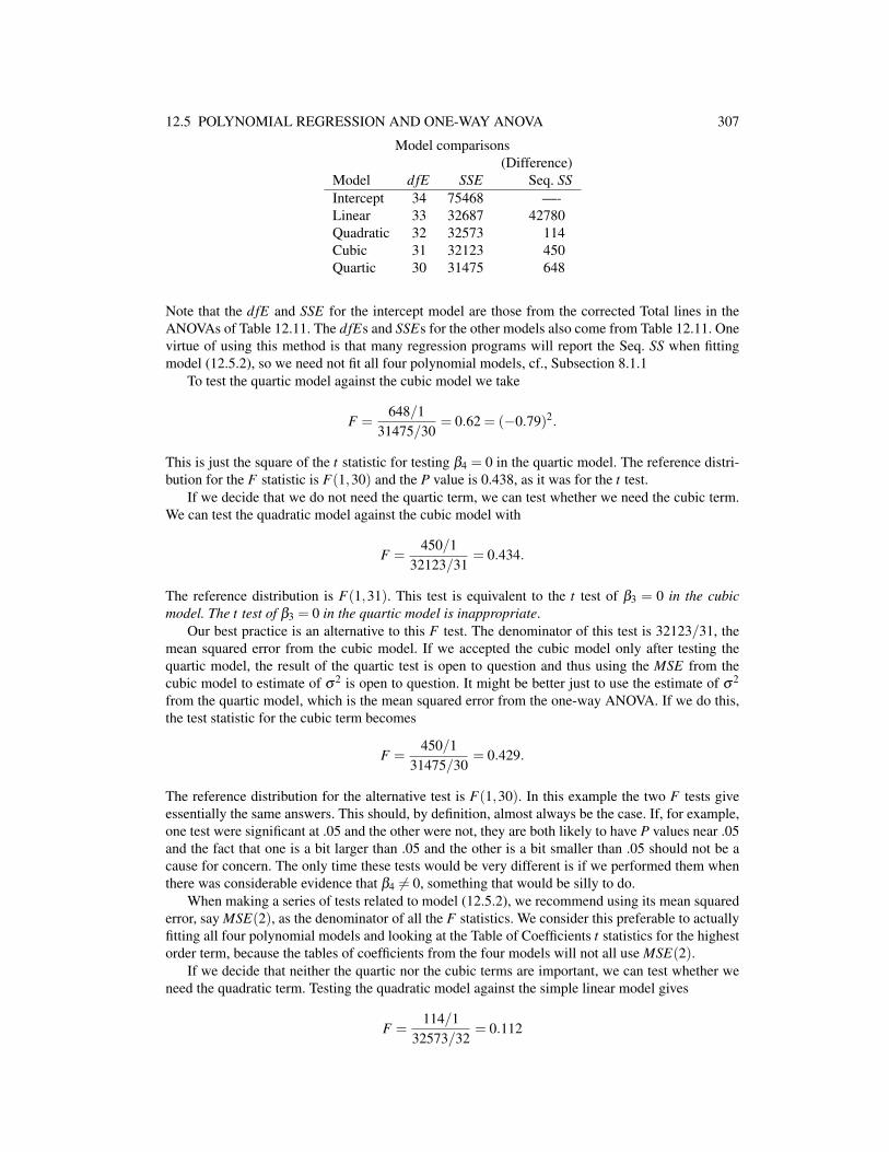
12.5 POLYNOMIAL REGRESSION AND ONE-WAY ANOVA 307
Model comparisons(Difference)
Model dfE SSE Seq. SSIntercept 34 75468 —-Linear 33 32687 42780Quadratic 32 32573 114Cubic 31 32123 450Quartic 30 31475 648
Note that the dfE and SSE for the intercept model are those from the corrected Total lines in theANOVAs of Table 12.11. The dfEs and SSEs for the other models also come from Table 12.11. Onevirtue of using this method is that many regression programs will report the Seq. SS when fittingmodel (12.5.2), so we need not fit all four polynomial models, cf., Subsection 8.1.1
To test the quartic model against the cubic model we take
F =648/1
31475/30= 0.62 = (−0.79)2.
This is just the square of the t statistic for testing β4 = 0 in the quartic model. The reference distri-bution for the F statistic is F(1,30) and the P value is 0.438, as it was for the t test.
If we decide that we do not need the quartic term, we can test whether we need the cubic term.We can test the quadratic model against the cubic model with
F =450/1
32123/31= 0.434.
The reference distribution is F(1,31). This test is equivalent to the t test of β3 = 0 in the cubicmodel. The t test of β3 = 0 in the quartic model is inappropriate.
Our best practice is an alternative to this F test. The denominator of this test is 32123/31, themean squared error from the cubic model. If we accepted the cubic model only after testing thequartic model, the result of the quartic test is open to question and thus using the MSE from thecubic model to estimate of σ2 is open to question. It might be better just to use the estimate of σ2
from the quartic model, which is the mean squared error from the one-way ANOVA. If we do this,the test statistic for the cubic term becomes
F =450/1
31475/30= 0.429.
The reference distribution for the alternative test is F(1,30). In this example the two F tests giveessentially the same answers. This should, by definition, almost always be the case. If, for example,one test were significant at .05 and the other were not, they are both likely to have P values near .05and the fact that one is a bit larger than .05 and the other is a bit smaller than .05 should not be acause for concern. The only time these tests would be very different is if we performed them whenthere was considerable evidence that β4 = 0, something that would be silly to do.
When making a series of tests related to model (12.5.2), we recommend using its mean squarederror, say MSE(2), as the denominator of all the F statistics. We consider this preferable to actuallyfitting all four polynomial models and looking at the Table of Coefficients t statistics for the highestorder term, because the tables of coefficients from the four models will not all use MSE(2).
If we decide that neither the quartic nor the cubic terms are important, we can test whether weneed the quadratic term. Testing the quadratic model against the simple linear model gives
F =114/1
32573/32= 0.112

308 12. ONE-WAY ANALYSIS OF VARIANCE
Table 12.12: Analysis of variance for ASI data.
(Seq.)Source df SS MS F PTreatments 4 43993 10998 10.48 0.000(linear) (1) (42780) (42780) (40.78)(quadratic) (1) ( 114) ( 114) (0.11)(cubic) (1) ( 450) ( 450) (0.43)(quartic) (1) ( 648) ( 648) (0.62)Error 30 31475 1049Total 34 75468
which is compared to an F(1,32) distribution. This test is equivalent to the t test of β2 = 0 in thequadratic model. Again, we prefer the quadratic term test statistic
F =114/1
31475/30= 0.109
with a reference distribution of F(1,30).If we decide that we need none of the higher order terms, we can test whether we need the linear
term. Testing the intercept model against the simple linear model gives
F =42780/132687/33
= 43.190.
This is just the test for zero slope in the simple linear model. Again, the preferred test for the linearterm has
F =42780/131475/30
= 40.775.
Table 12.12 contains an expanded analysis of variance table for the one-way ANOVA that in-corporates the information from this sequence of comparisons.
From Table 12.12, the P value of 0.000 indicates strong evidence that the five groups are differ-ent, i.e., there is strong evidence for the quartic polynomial helping to explain the data. The resultsfrom the sequential terms are so clear that we did not bother to report P values for them. There is ahuge effect for the linear term. The other three F statistics are all much less than 1, so there is noevidence of the need for a quartic, cubic, or quadratic polynomial. As far as we can tell, a line fits thedata just fine. For completeness, some residual plots are presented as Figures 12.7 through 12.11.Note that the normal plot for the simple linear regression in Figure 12.8 is less than admirable, whilethe normal plot for the one-way ANOVA in Figure 12.11 is only slightly better. It appears that oneshould not put great faith in the normality assumption. 2
12.5.1 Fisher’s lack-of-fit test
We now give a more extensive discussion of Fisher’s lack-of-fit test that was introduced in Sec-tion 8.5.
Comparing one of the reduced polynomial models against the one-way ANOVA model is oftenreferred to as a test of lack of fit. This is especially true when the reduced model is the simple linearregression model. In these tests, the degrees of freedom, sums of squares, and mean squares usedin the numerator of the tests are all described as being for lack of fit. The denominator of the testis based on the error from the one-way ANOVA. The mean square, sum of squares, and degrees offreedom for error in the one-way ANOVA are often referred to as the mean square, sum of squares,and degrees of freedom for pure error. This lack of fit test can be performed whenever the datacontain multiple observations at any x values. Often the appropriate unbalanced one-way ANOVA

12.5 POLYNOMIAL REGRESSION AND ONE-WAY ANOVA 309
4 6 8 10 12
−2−1
01
2
Residual−Plate Length plot
Plate Length
Stan
dard
ized r
esidu
als
Figure 12.8: ASI SLR standardized residuals versus plate length.
−2 −1 0 1 2
−2−1
01
2
Normal Q−Q Plot
Theoretical Quantiles
Stan
dard
ized r
esidu
als
Figure 12.9: ASI SLR standardized residuals normal plot, W ′ = .961.
includes groups with only one observation on them. These groups do not provide an estimate of σ2,so they simply play no role in obtaining the mean square for pure error. In Section 8.5 the Hookerdata had only two x values with multiple observations and both groups only had two observationsin them. Thus, the n = 31 cases are divided into a = 29 groups but only four cases were involved infinding the pure error.
For testing lack of fit in the simple linear regression model with the ASI data, the numeratorsum of squares can be obtained by differencing the sums of squares for error in the simple linearregression model and the one-way ANOVA model. Here the sum of squares for lack of fit is 32687−31475 = 1212 and the degrees of freedom for lack of fit are 33−30 = 3. The mean square for lack

310 12. ONE-WAY ANALYSIS OF VARIANCE
4 6 8 10 12
−2−1
01
2
Residual−Plate Length plot
Plate Length
Stan
dard
ized r
esidu
als
Figure 12.10: ASI ANOVA residuals versus plate length.
340 360 380 400 420 440
−2−1
01
2
Residual−Fitted plot
Fitted
Stan
dard
ized r
esidu
als
Figure 12.11: ASI ANOVA residuals versus predicted values.
of fit is 1212/3 = 404. The pure error comes from the one-way ANOVA table. The lack of fit test Fstatistic for the simple linear regression model is
F =404
1049= 0.39
which is less than 1, so there is no evidence of a lack of fit in the simple linear regression model. Ifan α = 0.05 test were desired, the test statistic would be compared to F(0.95,3,30).
A similar lack of fit test is available for any of the reduced polynomial models relative to theone-way ANOVA model.

12.6 WEIGHTED LEAST SQUARES 311
−2 −1 0 1 2
−2−1
01
2
Normal Q−Q Plot
Theoretical Quantiles
Stan
dard
ized r
esidu
als
Figure 12.12: ASI ANOVA residuals normal plot, W ′ = .965.
12.6 Weighted least squares
In general, weighted regression is a method for dealing with observations that have nonconstantvariances and nonzero correlations. In this section, we deal with the simplest form of weightedregression in which we assume zero correlations between observations. Weighted regression hassome interesting connections to fitting polynomials to one-way ANOVA data that we will examinehere and it has connections to analyzing the count data considered later.
Our standard regression model from Chapter 11 has
Y = Xβ + e, E(e) = 0, Cov(e) = σ2I.
We now consider a model for data that do not all have the same variance. In this model, we assumethat the relative sizes of the variances are known but that the variances themselves are unknown.In this simplest form of weighted regression, we have a covariance structure that changes fromCov(e) = σ2I to Cov(e) = σ2D(w)−1. Here D(w) is a diagonal matrix with known weights w =(w1, . . . ,wn)
′ along the diagonal. The covariance matrix involves D(w)−1, which is just a diagonalmatrix having diagonal entries that are 1/w1, . . . ,1/wn. The variance of an observation yi is σ2/wi.If wi is large relative to the other weights, the relative variance of yi is small, so it contains moreinformation than other observations and we should place more weight on it. Conversely, if wi isrelatively small, the variance of yi is large, so it contains little information and we should place littleweight on it. For all cases, wi is a measure of how much relative weight should be placed on case i.Note that the weights are relative, so we could multiply or divide them all by a constant and obtainessentially the same analysis. Obviously, in standard regression the weights are all taken to be 1.
In matrix form, our new model is
Y = Xβ + e, E(e) = 0, Cov(e) = σ2D(w)−1. (12.6.1)
In this model all the observations are uncorrelated because the covariance matrix is diagonal. Wedo not know the variance of any observation because σ2 is unknown. However, we do know therelative sizes of the variances because we know the weights wi. It should be noted that when model(12.6.1) is used to make predictions, it is necessary to specify weights for any future observations.
Before giving a general discussion of weighted regression models, we examine some examples

312 12. ONE-WAY ANALYSIS OF VARIANCE
of their application. A natural application of weighted regression is to data for a one-way analysisof variance with groups that are quantitative levels of some factor. With a quantitative factor, we canperform either a one-way ANOVA or a regression on the data. However, if for some reason the fulldata are not available, we can still obtain an appropriate simple linear regression by performing aweighted regression analysis on the treatment means. The next examples explore the relationshipsbetween regression on the full data and weighted regression on the treatment means.
In the weighted regression, the weights turn out to be the treatment group sample sizes fromthe ANOVA. In a standard unbalanced ANOVA yi j = µi +εi j, i = 1, . . . ,a, j = 1, . . . ,Ni, the samplemeans have Var(yi·) = σ2/Ni. Thus, if we perform a regression on the means, the observationshave different variances. In particular, from our earlier discussion of variances and weights, it isappropriate to take the sample sizes as the weights, i.e., wi = Ni.
EXAMPLE 12.6.1. In Section 12.5 we considered the axial stiffness data of Table 12.9. A simplelinear regression on the full data gives the following
Table of Coefficients: SLRPredictor βk SE(βk) t PConstant 285.30 15.96 17.88 0.000x (plates) 12.361 1.881 6.57 0.000
The analysis of variance table for the simple linear regression is given below. The usual errorline would have 33 degrees of freedom but, as per Subsection 12.5.1, we have broken this into twocomponents, one for lack of fit and one for pure error.
Analysis of Variance: SLRSource df SS MSRegression 1 42780 42780Lack of fit 3 1212 404Pure error 30 31475 1049Total 34 75468
In Section 12.5 we presented group summary statistics, yi· and s2i , for the four plate lengths. The
mean squared pure error is just the pooled estimate of the variance and the sample sizes and samplemeans are given below.
Plate 4 6 8 10 12N 7 7 7 7 7yi· 333.2143 368.0571 375.1286 407.3571 437.1714
As mentioned in Section 12.5, one can get the same estimated line by just fitting a simple linearregression to the means. For an unbalanced ANOVA, getting the correct regression line from themeans requires a weighted regression. In this balanced case, if we use a weighted regression we getnot only the same fitted line but also some interesting relationships in the ANOVA tables. Beloware given the Table of Coefficients and the ANOVA table for the weighted regression on the means.The weights are the sample sizes for each mean.
Table of Coefficients: Weighted SLRPredictor βk SE(βk) t PConstant 285.30 10.19 27.99 0.000x (plates) 12.361 1.201 10.29 0.002
Analysis of Variance: Weighted SLRSource df SS MS F PRegression 1 42780 42780 105.88 0.002Error 3 1212 404Total 4 43993

12.6 WEIGHTED LEAST SQUARES 313
The estimated regression coefficients are identical to those given in Section 12.5. The standard errorsand thus the other entries in the table of coefficients differ. In the ANOVA tables, the regressionlines agree while the error line from the weighted regression is identical to the lack of fit line inthe ANOVA table for the full data. In the weighted regression, all standard errors use the lack of fitas an estimate of the variance. In the regression on the full data, the standard errors use a varianceestimate obtained from pooling the lack of fit and the pure error. The ultimate point is that by usingweighted regression on the summarized data, we can still get most relevant summary statistics forsimple linear regression. Of course, this assumes that the simple linear regression model is correct,and unfortunately the weighted regression does not allow us to test for lack of fit.
If we had taken all the weights to be one, i.e., if we had performed a standard regression on themeans, the parameter estimate table would be the same but the ANOVA table would not display theidentities discussed above. The sums of squares would all have been off by a factor of 7. 2
Minitab commands
To get the weighted regression from Minitab, suppose that c1 contains the plate lengths, c2 containsthe sample sizes, and c3 contains the means. The commands are as follows:
MTB > regress c3 on 1 c1;
SUBC> weights c2.
A complete set of commands for generating an analysis such as this are given for the next example.
Unbalanced weights
We now examine an unbalanced one-way ANOVA and again compare a simple linear regressionincluding identification of pure error and lack of fit to a weighted regression on sample means.
EXAMPLE 12.6.2. Consider the data of Exercise 6.11.1 and Table 6.8. These involve ages oftruck tractors and the costs of maintaining the tractors. A simple linear regression on the full datayields the tables given below.
Table of Coefficients: SLRPredictor βk SE(βk) t PConstant 323.6 146.9 2.20 0.044Age 131.72 35.61 3.70 0.002
Analysis of Variance: SLRSource df SS MSRegression 1 1099635 1099635Lack of fit 5 520655 104131Pure error 10 684752 68475Total 16 2305042
The weighted regression analysis is based on the sample means and sample sizes given below.The means serve as the y variable, the ages are the x variable, and the sample sizes are the weights.
Age 0.5 1.0 4.0 4.5 5.0 5.5 6.0Ni 2 3 3 3 3 1 2yi· 172.5 664.3 633.0 900.3 1202.0 987.0 1068.5
The Table of Coefficients and ANOVA table for the weighted regression are
Table of Coefficients: Weighted SLRPredictor βk SE(βk) t PConstant 323.6 167.3 1.93 0.111Age 131.72 40.53 3.25 0.023

314 12. ONE-WAY ANALYSIS OF VARIANCE
and
Analysis of Variance: Weighted SLRSource df SS MS F PRegression 1 1099635 1099635 10.56 0.023Error 5 520655 104131Total 6 1620290
Note that, as in the previous example, the regression estimates agree with those from the full data,that the regression sum of squares from the ANOVA table agrees with the full data, and that the lackof fit line from the full data ANOVA agrees with the error line from the weighted regression. For anunbalanced ANOVA, you cannot obtain a correct simple linear regression analysis from the groupmeans without using weighted regression. 2
Minitab commands
The Minitab commands for this analysis are given below. To obtain pure error and lack of fit fromthe full data one fits both the simple linear regression and the one-way ANOVA. The ages fromTable 7.14 are in c1 and the costs are in c2.
MTB > regress c2 on 1 c1
MTB > note THE AGES IN c1 ARE NOT INTEGERS, SO WE
MTB > note MULTIPLY THEM BY TWO TO MAKE INTEGER
MTB > note GROUP LABELS FOR THE ONE-WAY
MTB > let c3=2*c1
MTB > oneway c2 c3
MTB > note PUT THE MEANS FROM THE ONE-WAY INTO c6, THE
MTB > note AGES INTO c7, AND THE SAMPLE SIZES INTO c8.
MTB > set c6
DATA> 172.5 664.333333 633 900.3333333 1202 987 1068.5
DATA> set c7
DATA> .5 1 4 4.5 5 5.5 6
DATA> end
MTB > set c8
DATA> 2 3 3 3 3 1 2
DATA> end
MTB > note DO THE WEIGHTED REGRESSION
MTB > regress c6 on 1 c7;
SUBC> weight c8.
Theory
The analysis of the weighted regression model (12.6.1) is based on changing it into a standardregression model. The trick is to create a new diagonal matrix that has entries
√wi. In a minor abuse
of notation, we write this matrix as D(√
w). We now multiply model (12.6.1) by this matrix to obtain
D(√
w)Y = D(√
w)Xβ +D(√
w)e. (12.6.2)
It is not difficult to see that
E(D(
√w)e)= D(
√w)E(e) = D(
√w)0 = 0
andCov
(D(
√w)e)= D(
√w)Cov(e)D(
√w)′ = D(
√w)[σ2D(w)−1]D(
√w) = σ2I.

12.7 EXERCISES 315
Table 12.13: Rubber stress at five laboratories.
Sample Sample SampleLab. size mean variance1 4 57.00 32.002 4 67.50 46.333 4 40.25 14.254 4 56.50 5.665 4 52.50 6.33
Thus equation (12.6.2) defines a standard regression model. For example, by Proposition 11.3.1 theleast squares regression estimates from model (12.6.2) are
β =([D(
√w)X ]′[D(
√w)X ]
)−1[D(
√w)X ]′[D(
√w)Y ]
= (X ′D(w)X)−1X ′D(w)Y.
The estimate of β given above is referred to as a weighted least squares estimate because rather thanminimizing [Y −Xβ ]′ [Y −Xβ ], the estimates are obtained by minimizing[
D(√
w)Y −D(√
w)Xβ]′ [
D(√
w)Y −D(√
w)Xβ]= [Y −Xβ ]′ D(w) [Y −Xβ ] .
Thus the original minimization problem has been changed into a similar minimization problem thatincorporates the weights. The sum of squares for error from model (12.6.2) is
SSE =[D(
√w)Y −D(
√w)X β
]′ [D(
√w)Y −D(
√w)X β
]=[Y −X β
]′D(w)
[Y −X β
].
The dfE are unchanged from a standard model and MSE is simply SSE divided by dfE. Standarderrors are found in much the same manner as usual except now
Cov(
β)= σ2(X ′D(w)X)−1.
Because the D(w) matrix is diagonal, it is very simple to modify a computer program for stan-dard regression to allow the analysis of models like (12.6.1). Of course to make a prediction, aweight must now be specified for the new observation. Essentially the same idea of rewriting model(12.6.1) as the standard regression model (12.6.2) works even when D(w) is not a diagonal matrix,cf. Christensen (2011, Sections 2.7 and 2.8).
12.7 Exercises
EXERCISE 12.7.1. In a study of stress at 600% elongation for a certain type of rubber, Mandel(1972) reported stress test data from five different laboratories. These data are distinct from Ta-ble 12.4. Summary statistics are given in Table 12.6. Compute the analysis of variance table and testfor differences in means between all pairs of labs. Use α = .01. Is there any reason to worry aboutthe assumptions of the analysis of variance model?
EXERCISE 12.7.2. Snedecor and Cochran (1967, section 6.18) presented data obtained in 1942from South Dakota on the relationship between the size of farms (in acres) and the number ofacres planted in corn. Summary statistics are presented in Table 12.7. Note that the sample standarddeviations rather than the sample variances are given. In addition, the pooled standard deviation is0.4526.

316 12. ONE-WAY ANALYSIS OF VARIANCE
Table 12.14: Acreage in corn for different sized farms.
Farm Sample Sample Sampleacres size mean std. dev.
80 5 2.9957 0.4333160 5 3.6282 0.4056240 5 4.1149 0.4169320 5 4.0904 0.4688400 5 4.4030 0.5277
Table 12.15: Weights (in pounds) for various heights (in inches).
Sample Sample SampleHeight size mean variance
63 3 121.66 158.33365 4 131.25 72.91366 2 142.50 112.50072 3 171.66 158.333
(a) Give the one-way analysis of variance model with all of its assumptions. Can any problems withthe assumptions be identified?
(b) Give the analysis of variance table for these data. Test whether there are any differences in cornacreages due to the different size farms. Use α = .01.
(c) Test for differences between all pairs of farm sizes using α = .01 tests.(d) Find the sum of squares for the following contrast:
Farm 80 160 240 320 400Coeff. −2 −1 0 1 2
What percentage is this of the treatment sum of squares?e) Give 95% confidence and prediction intervals for the number of acres in corn for each farm
size.
EXERCISE 12.7.3. Table 12.8 gives data on heights and weights of people. Give the analysis ofvariance table and test for differences among the four groups. Give a 99% confidence interval forthe mean weight of people in the 72 inch height group.
EXERCISE 12.7.4. Conover (1971, p. 326) presented data on the amount of iron found in thelivers of white rats. Fifty rats were randomly divided into five groups of ten and each group wasgiven a different diet. We analyze the logs of the original data. The total sample variance of the 50observations is 0.521767 and the means for each diet are given below.
Diet A B C D EMean 1.6517 0.87413 0.89390 0.40557 0.025882
Compute the analysis of variance table and test whether there are differences due to diet.If diets A and B emphasize beef and pork respectively, diet C emphasizes poultry, and diets D
and E are based on dried beans and oats, the following contrasts may be of interest.

12.7 EXERCISES 317
Table 12.16: Peel-strength of various adhesive systems.
Adhesivesystem Observations
1 60 63 57 53 56 572 57 52 55 59 56 543 19.8 19.5 19.7 21.6 21.1 19.34 52 53 44 48 48 53
DietContrast A B C D EBeef vs. pork 1 −1 0 0 0Mammals vs. poultry 1 1 −2 0 0Beans vs. oats 0 0 0 1 −1Animal vs. vegetable 2 2 2 −3 −3
Show that the contrasts are orthogonal and compute sums of squares for each contrast. Interpretyour results and draw conclusions about the data.
EXERCISE 12.7.5. In addition to the data discussed earlier, Mandel (1972) reported data fromone laboratory on four different types of rubber. Four observations were taken on each type ofrubber. The means are given below.
Material A B C DMean 26.4425 26.0225 23.5325 29.9600
The sample variance of the 16 observations is 14.730793. Compute the analysis of variance table,the overall F test, and test for differences between each pair of rubber types. Use α = .05.
EXERCISE 12.7.6. In Exercise 12.7.5 on the stress of four types of rubber, the observations onmaterial B were 22.96, 22.93, 22.49, and 35.71. Redo the analysis, eliminating the outlier. Thesample variance of the 15 remaining observations is 9.3052838.
EXERCISE 12.7.7. Bethea et al. (1985) reported data on an experiment to determine the effec-tiveness of four adhesive systems for bonding insulation to a chamber. The data are a measure ofthe peel-strength of the adhesives and are presented in Table 12.9. A disturbing aspect of these datais that the values for adhesive system 3 are reported with an extra digit.
(a) Compute the sample means and variances for each group. Give the one-way analysis of variancemodel with all of its assumptions. Are there problems with the assumptions? If so, does ananalysis on the square roots or logs of the data reduce these problems?
(b) Give the analysis of variance table for these (possibly transformed) data. Test whether there areany differences in adhesive systems. Use α = .01.
(c) Test for differences between all pairs of adhesive systems using α = .01 tests.(d) Find the sums of squares i) for comparing system 1 with system 4 and ii) for comparing system
2 with system 3.(e) Perform a .01 level F test for whether the mean peel-strength of systems 1 and 4 differs from the
mean peel-strength of systems 2 and 3.(f) What property is displayed by the sums of squares computed in (d) and (e)? Why do they have
this property?(g) Give a 99% confidence interval for the mean of every adhesive system.

318 12. ONE-WAY ANALYSIS OF VARIANCE
Table 12.17: Weight gains of rats.
Thyroxin Thiouracil Control132 68 68 107 115
84 63 52 90 117133 80 80 91 133118 63 61 91 115
87 89 69 112 9588
119
Table 12.18: Tetrahydrocortisone values for patients with Cushing’s syndrome.
a b c3.1 8.3 15.4 10.23.0 3.8 7.7 9.21.9 3.9 6.5 9.63.8 7.8 5.7 53.84.1 9.1 13.6 15.81.9
(h) Give a 99% prediction interval for every adhesive system.(i) Give a 95% confidence interval for the difference between systems 1 and 2.
EXERCISE 12.7.8. Table 12.10 contains weight gains of rats from Box (1950). The rats weregiven either Thyroxin or Thiouracil or were in a control group. Do a complete analysis of varianceon the data. Give the model, check assumptions, make residual plots, give the ANOVA table, andexamine appropriate contrasts.
EXERCISE 12.7.9. Aitchison and Dunsmore (1975) presented data on Cushing’s syndrome.Cushing’s syndrome is a condition in which the adrenal cortex overproduces cortisol. Patients aredivided into one of three groups based on the cause of the syndrome: a – adenoma, b – bilateralhyperplasia, and c – carcinoma. The data are amounts of tetrahydrocortisone in the urine of thepatients. The data are given in Table 12.11. Give a complete analysis.
EXERCISE 12.7.10. Draper and Smith (1966, p. 41) considered data on the relationship betweenthe age of truck tractors (in years) and the cost (in dollars) of maintaining them over a six monthperiod. The data are given in Table 12.12.
Note that there is only one observation at 5.5 years of age. This group does not yield an estimateof the variance and can be ignored for the purpose of computing the mean squared error. In theweighted average of variance estimates, the variance of this group is undefined but the variance gets0 weight, so there is no problem.
Table 12.19: Age and costs of maintenance for truck tractors.
Age Costs0.5 163 1821.0 978 466 5494.0 495 723 6814.5 619 1049 10335.0 890 1522 11945.5 9876.0 764 1373

12.7 EXERCISES 319
Give the analysis of variance table for these data. Does cost differ with age? Is there a significantdifference between the cost at 0.5 years as opposed to 1.0 year? Use several contrasts to determinewhether there are any differences between costs at 4, 4.5, 5, 5.5, and 6 years. How much of the sumof squares for groups is due to the following contrast?
Age 0.5 1.0 4.0 4.5 5.0 5.5 6.0Coeff. −5 −5 2 2 2 2 2
What is the sum of squares for the contrast that compares the average of 0.5 and 1.0 with theaverages of 4, 4.5, 5, 5.5, and 6?
EXERCISE 12.7.11. George Snedecor (1945a) asked for the appropriate variance estimate in thefollowing problem. One of six treatments was applied to the 10 hens contained in each of 12 cages.Each treatment was randomly assigned to two cages. The data were the number of eggs laid by eachhen.
(a) What should you tell Snedecor? Were the treatments applied to the hens or to the cages? Howwill the analysis differ depending on the answer to this question?
(b) The mean of the 12 sample variances computed from the 10 hens in each cage was 297.8. Theaverage of the 6 sample variances computed from the two cage means for each treatment was57.59. The sample variance of the 6 treatment means was 53.725. How should you construct anF test? Remember that the numbers reported above are not necessarily mean squares.
EXERCISE 12.7.12. Lehmann (1975), citing Heyl (1930) and Brownlee (1960), considered dataon determining the gravitational constant of three elements: gold, platinum, and glass. The dataLehmann gives are the third and fourth decimal places in five determinations of the gravitationalconstant. They are presented below. Analyze the data.
Gold Platinum Glass83 61 7881 61 7176 67 7579 67 7276 64 74
EXERCISE 12.7.13. Shewhart (1939, p. 69) also presented the gravitational constant data of Heyl(1930) that was considered in the previous problem, but Shewhart reports six observations for goldinstead of five. Shewhart’s data are given below. Analyze these data and compare your results tothose of the previous exercise.
Gold Platinum Glass83 61 7881 61 7176 67 7579 67 7278 64 7472
EXERCISE 12.7.14. Recall that if Z ∼ N(0,1) and W ∼ χ2(r) with Z and W independent, thenby Definition 2.1.3 Z
/√W/r has a t(r) distribution. Also recall that in a one-way ANOVA with
independent normal errors, a contrast has
a
∑i=1
λiyi· ∼ N
(a
∑i=1
λiµi,σ2a
∑i=1
λ 2i
Ni
),

320 12. ONE-WAY ANALYSIS OF VARIANCESSEσ2 ∼ χ2(dfE),
and MSE independent of all the yi·s. Show that
∑ai=1 λiyi·−∑a
i=1 λiµi√MSE ∑a
i=1 λ 2i /Ni
∼ t(dfE).
EXERCISE 12.7.15. Suppose a one-way ANOVA involves four diet treatments: Control, Beef A,Beef B, Pork, and Beans. As in Subsection 12.4.1, construct a reasonable hierarchy of models toexamine that involves five rows and no semicolons.
EXERCISE 12.7.16. Suppose a one-way ANOVA involves four diet treatments: Control, Beef,Pork, Lima Beans, and Soy Beans. As in Subsection 12.4.1, construct a reasonable hierarchy ofmodels that involves four rows one of which involves a semicolon.