CHAPTER 11

INSTABILITY IN ROTATING MACHINES

In the most of previous chapters, except Chapter 3, we studied how to obtain the free and forced

responses of rotor-bearing systems in different modes of vibrations (e.g., the torsional, transverse, and

axial vibrations). Main aims of these chapters were to obtain natural whirl frequencies, mode shapes,

critical speeds and unbalance response. Unbalance response analysis presented can be extended to

other types of periodic forces with the help of Fourier series especially for the linear systems, where

the principle of superposition holds good. Various methods especially suited for analyzing complex

rotor systems (apart from general methods of vibration analysis, like the Newton’s second law of

motion, Lagrange’s method, Hamilton’s principle, etc.) have been dealt in great detail from its

fundamentals (e.g., the transfer matrix and finite element methods). Now in next few chapters, we

would explore another kind of phenomena in rotor-bearing systems called the instability, which might

cause the catastrophic failure of the systems. In certain circumstances, depending upon the design,

some machine may be prone to instability. This means that machine vibrations set in, even in the

absence of unbalance effects, resulting in high levels of noise and component stress and a

corresponding reduced fatigue life. In linear systems the magnitude of these vibrations tends towards

infinity, although in practice shaft vibrations are often limited by system non-linearity. In the present

chapter, various kinds of instability will be studies. Such machine instabilities may originate from a

number of sources including fluid-film bearings, seals, shaft stiffness asymmetry, internal friction

between mating components, and aerodynamic forces. A designer’s problem is to investigate the

possibility of machine instability, and to change the appropriate machine design parameters to ensure

that may potential unstable modes of operation lie outside the normal operating regime of the

machine. Apart from these when rotors are subjected to angular accelerations (uniform or variable

depending upon the unlimted or limited power of the drive, respectively), transient responses are

generated and study of such transient response is of practical importance. The aim of the present

chapter is to understand various kinds of instability with a simple single mass rotor model and in some

cases with a continuous shaft model. In the subsequent chapter, we would explore methods of

predicting instability in large rotor-bearing systems especially with finite element methods.

11.1 Oil Whirl

In rotating machineries, the unbalance is the most common source of excitation, which comes from

rotors. Similarly, oil-film bearings are possibly the most common source of instability in such rotating

machineries. Oil-whirl instability is also known as ‘half-speed whirl’ because the frequency of whirl

(vibrations) which are set up is often just below half the shaft rotational frequency (typically 0.46-0.48

654

times of shaft rotational frequency). This instability tends to occur only in lightly loaded oil-film

bearings operating at a very small eccentricity ratio ( /r re c , where er is the eccentricity of the rotor

centre with respect to the bearing centre and cr is the radial clearance). It is an externally dangerous

condition because bearing load-carrying decreases and results in very high whirl amplitude and

consequently the destruction of the bearings is a possibility. Let us consider an fluid-film bearing in

which journal is rotating with frequency, ω , and whirls around the bearing clearance (i.e., er) at

frequency ωn as shown in Figure 11.1. Because the bearing is lightly loaded (so operates at only a

small eccentricity er in the first instance) the variation in fluid pressure around the bearing

circumference may be considered to be negligible so that the only fluid flows around the bearing the

bearing is that which is induced by the rotation of the journal. The lubricant flow rate into, and out of,

the dotted wedge-shaped are as shown in Figure 11.1(a) is the given by

12 ( 0)( )in r rQ R c eω= + + and 1

2 ( 0)( )out r rQ R c eω= + − (11.1)

where inQ ( 12 ( 0)Rω + is the average velocity and ( )r rc e+ is the passage width) and outQ (

)0(21 +ωR is the average velocity and ( )r rc e− is the passage width) are flow per unit length of the

bearing.

(a) Journal and lubricant in a bearing during oil whirl (b) The whirl orbit of the shaft centre

Figure 11.1 Oil whirl in fluid film bearings

Since journal is whirling within the bearing clearance with some frequency ωn , the tangential

velocity of the journal center will be rn eω as shown in Figure 11.1(b). So the volume of dotted area,

per unit length of the bearing must be increasing at a rate given by

( )(2 )vol rQ n e Rω= (11.2)

655

where ( )rn eω is the tangential velocity of journal center and )2( R is the shaded area of journal per

unit length of bearing. The volume flow rate must be provided by the net lubricant flow into the

dotted are under consideration, so that we may write

voloutin QQQ =− (11.3)

On substituting equations (11.1) and (11.2) into equation (11.3), we get

1 1

2 2( ) ( ) 2r r r r rR c e R c e Rn eω ω ω+ − − =

or

( ) ( ) 4r r r r rc e c e ne+ − − = 2 4r re ne� = (11.4)

which gives 5.0=n . So the frequency of whirl is half the rotational frequency of journal. The

deviation from the actual case (0.46� to 0.48�) is due to the assumption made in the analysis

regarding no flow due to pressure variation across the circumference of the bearing.

Example 11.1: Let us consider two identical bearings which are symmetrically supporting a light

symmetrical rotor at its ends. Through measurement the following data were found: the bore of the

journal bearing is 3 cm with the radial clearance of 5 mµ , and the rotor spin speed is 3000 rpm. The

flow measurement were 52.827 10iQ −= × m3/s and 51.885 10outQ −= × m3/s. If the rotor is under the

half-speed whirl, obtain the eccentricity ratio of the rotor centre in the journal.

Solution: We have the following data

3R = cm, 65 10rc −= × m, 2 3000

314.1660

πω ×= = rad/s

52.827 10iQ −= × m3/s, 51.885 10outQ −= × m3/s

From equation (11.4), we have

2in out rQ Q Rn eω− =

Hence the eccentricity ratio can be written as

656

( ) 5

6

2.827 1.885 10

2 2 0.03 0.5 314.16 5 10in outr

r r

Q Qec Rn c

εω

−

−

− ×−= = = =× × × × ×

0.2

Hence, it has very low eccentricity ratio.

11.2 Stability Analysis using Linearized Stiffness and Damping Coefficients

A stable rotor-bearing may be defined as one that will have a bounded response for all possible

bounded excitations. To investigate the likelihood of oil whirl, attention needs to be given to the

bearing operating characteristics. For oil-film bearings these may be expressed in terms of the eight-

linearised stiffness and damping coefficients.

(a) A rotor-bearing system with bearing forces

(b) Free body diagram in y-z plane (c) Free body diagram in z-x plane

Figure 11.2 A rigid rotor mounted on two identical anisotropic bearings

The relationship between the bearing forces and the journal motion is given by the equations of

motion of the journal, which in the case of symmetrical system with a rigid rotor (Fig. 11.2), case are

xx xy xx xy

yx yy yx yy

k x k y c x c y mx

k x k y c x c y my

+ + + = −

+ + + = −

� � ��

� � ��

(11.5)

where x and y are the horizontal and vertical displacements of the rotor, k’s and c’s are stiffness and

damping coefficients, and m is the half of the rotor mass. Here it is assumed that a rigid rotor is

mounted on two identical fluid-film bearings and has a purely translational motion. If the rotor is

657

momentarily displaced from its equilibrium position by some random input, free vibrations of the

rotor in the horizontal and vertical directions will take the form

0tx X eλ= and 0

ty Y eλ= (11.6)

where λ is a parameter and in general it is a complex quantity with the real part represent the

damping and the imaginary part as the whirl natural frequency; and 0X and 0Y are the vibration

amplitudes in the horizontal and vertical directions, respectively. Equation (11.6) gives

0tx X eλλ=� ; 0

ty X eλλ=� ; 20

tx X eλλ=�� ; 20

ty X eλλ=�� (11.7)

On substituting equations (11.6) and (11.7) into equation (11.5), and dividing whole equation by teλ ,

we get

20 0 0 0 0

20 0 0 0 0

( )

( )

xx xy xx xy

yx yy yx yy

k X k Y c X c Y m X

k X k Y c X c Y m Y

λ λ λ

λ λ λ

+ + + = −

+ + + = − (11.8)

which can be simplified as

20 0

20 0

( ) ( )

( ) ( )

xx xx xy xy

yx yx yy yy

X m k c Y k c

X k c Y m k c

λ λ λ

λ λ λ

− − − = +

+ = − − − (11.9)

Equation (11.9) can be combined as

2

02

0

xy xy yy yy

xx xx yx yx

c k m c kXY m c k c k

λ λ λλ λ λ

+ + += − = −

+ + +

(11.10)

which gives the frequency equation as

658

2 4 3 2( ) ( ) ( )

( ) ( ) 0

xx yy xy yy xx yy xy yx

yx xx yy xx xy yx xy yx xx yy xy yx

m m c c mk mk c c c c

k c c k k c c k k k k k

λ λ λ

λ

+ + + + + −

+ + − − + − = (11.11)

The most direct approach for investigating the stability of a linear rotor-bearing system is to determine

the roots of the above characteristic polynomial (i.e., the frequency equation). Equation (11.11) has

four roots of λ . In general the roots of λ will both real and imaginary parts, indicating that the

transient motion of the journal will take a form of harmonic wave having decaying amplitude when

the system is stable (i.e., when the real parts of all roots of λ are negative). The imaginary parts of the

roots of λ indicate the frequency of the resulting vibrations.

Physically to test for the system stability one must examine the motion of the journal which follows a

momentary displacement from its steady running position. Does the journal return to a stable

equilibrium or not? If the journal were to return to a stable equilibrium position then this would be

characterized by values of displacement x and y which decreases with time, that is by negative values

of Re(�). If the journal motion is unbounded with time that means a positive value of Re(�). The

circumstances under which the real parts of all roots of � are negative are given by the Routh-Hurwitz

stability criteria. This criterion was developed independently by Hurwitz (1895) in Germany and

Routh (1892) in United States. Two approaches are presented in which the first one determines the

stability of the system with the help of Routh table (Sinha, 1995)) and the second one finds by a set of

dominants.

Method 1: Let the characteristic polynomial be given by

( ) 1 1 2 4 3 21 1 2 4 3 2 1 0

n n n nn n n na a a a a a a a aλ λ λ λ λ λ λ λ λ+ − −

+ − −∆ = + + + + + + + + + +� (11.12)

Then the Routh table (Table 11.1) is constructed based on the coefficients of the polynomial. The

Routh-Hurwitz criterion states that the number of roots with positive real parts is equal to the number

of changes in sign in the first column of the Routh table. Hence, for the system to be stable, no sign

changes should take place in the first column of the table.

659

Table 11.1 Routh table for finding the stability of a linear rotor-bearing system 1nλ + 1na + 1na − 3na − �

nλ na 2na − 4na − �

1nλ − ( )1 1 2n n n nn

n

a a a ab

a− + −−

= ( )3 1 4

1n n n n

nn

a a a ab

a− + −

−

−=

( )5 1 62

n n n nn

n

a a a ab

a− + −

−

−=

�

2nλ − ( )2 1n n n nn

n

b a a bc

b− −−

= ( )4 2

1n n n n

nn

b a a bc

b− −

−

−=

( )6 32

n n n nn

n

b a a bc

b− −

−

−=

�

� � � � 0λ hn

Method 2: For the stability of a linear system the following conditions are to be met (i) all

coefficients of the characteristic equation must have the same sign, and (ii) each of the following

determinants must be positive

11 aR = , 23

012 aa

aaR = ,

345

123

01

3

0

aaaaaa

aa

R = ,

4567

1345

0123

01

4

00

aaaa

aaaa

aaaa

aa

R = , …

nnnnnnn

n

aaaaaaa

aaaaaa

aaaaaa

aaaaaa

aaaa

aa

R

�

��������

�

�

�

�

�

625242322212

456789

234567

012345

0123

01

000

00000000

−−−−−−

= (11.13)

where system characteristics equation takes the form

1 4 3 2

1 4 3 2 1 0 0n nn na a a a a a aλ λ λ λ λ λ+

+ + + + + + + + =� (11.14)

Substitution of appropriate values into equation (11.7) then allows the designer to determine whether

a machine is likely to be stable or unstable. It does not indicate how stable (or unstable) a machine

may be. It will be noted from above that system stability depends upon the stiffness and damping of

bearings. Hence, for equation (11.11), we have the following stability conditions

660

( ) 0, ( ) 0,

( ) 0, ( ) 0

xx yy xy yy xx yy xy yx

yx xx xx yy xy yx yx xy xx yy xy yx

m c c mk mk c c c c

k c k c k c k c k k k k

+ ≥ + + − ≥

+ − − ≥ − ≥ (11.15)

and

2 1 2 0 3

( )( ) ( )( ) 0yx xx xx yy xy yx yx xy xy yy xx yy xy yx xx yy xy yx xx yy

R a a a a

k c k c k c k c mk mk c c c c m k k k k c c

= −= + − − + + − − − + ≥

( )( ) ( )( ) ( ) ( ) ( )

2 23 1 2 3 1 4 0 3

2 22

0

yx xx xx yy xy yx yx xy xy yy xx yy xy yx xx yy

yx xx xx yy xy yx yx xy xx yy xy yx xx yy

R a a a a a a a

k c k c k c k c mk mk c c c c m c c

k c k c k c k c m k k k k m c c

= − −

= + − − + + − +

− + − − − − + ≥

(11.16)

Example 11.2 For a rigid rotor of mass 10 kg is supported on two identical fluid film bearings with

the following properties: kxx = 20 MN/m, kyy = 15 MN/m, kxy = -1.5 MN/m, kyx = 25 MN/m, cxx = 200

kN-s/m, cxy = 150 kN-s/m, cyx = 140 kN-s/m and cyy = 400 kN-s/m. Find the stability of the rotor.

Solution: Half of the mass of the rotor m = 5kg. On substituting the given rotor and bearing properties

in equation (11.11), we get

4 3 3 6 225 5 (200 400) 10 ( 5 1.5 5 15 200 400 150 140) 10λ λ λ+ × + × + − × + × + × − × ×

9 12(25 200 20 400 1.5 140 25 150) 10 (20 15 1.5 25) 10 0λ+ × + × + × − × × + × + × × = (a)

On simplification of equation (a), we get

4 6 3 10 2 12 1425 3 10 5.91 10 9.46 10 3.38 10 0λ λ λ λ+ × + × + × + × = (b)

Equation has the following form

4 3 2

4 3 2 1 0 0a a a a aλ λ λ λ+ + + + = (c)

Method 1: The Routh table for the above characteristic equation is given in Table 11.2. Since the

degree of polynomial is 4 (n + 1 = 4), hence n = 3. It can be observed that there is no sign change in

the first column of the Routh table and hence the system is in stable condition.

Table 11.2 Routh table for finding the stability of a linear rotor-bearing system (n = 3)

661

4λ 4 25a = 2a = 5.91×1010 0a = 3.38×1014

3λ 3a = 3×106 1a = 9.46×1012 1a− = 0

2λ ( )3 2 4 23

3

a a a ab

a

−=

= 5.902×1010

( )3 0 4 12 0

3

a a a ab a

a−−

= =

= 3.38×1014

( )3 2 4 31

3

0a a a a

ba

− −−= =

1λ ( )3 1 3 23

3

b a a bc

b

−=

= 9.443×1012

( )3 1 3 12

3

0b a a b

cb

− −= =

( )3 3 3 01

3

0b a a b

cb

− −= =

0λ ( )3 2 3 23

3

c b b cd

c

−=

= 3.38×1014

2 0d = 1 0d =

Method 2: Hence, the first condition of stability is satisfied, i.e., all coefficients of the characteristic

equation must have the same sign. The second condition is that the following determinant must be

positive:

121 1 9.46 10R a= = × ,

12 141 0 23

2 6 103 2

9.46 10 3.38 105.58 10

3.00 10 5.91 10

a aR

a a× ×

= = = ×× ×

,

12 141 0

6 10 12 303 3 2 1

65 4 3

0 9.46 10 3.38 10 0.003.00 10 5.91 10 9.46 10 1.67 10

0.00 25.00 3.00 10

a a

R a a a

a a a

× ×= = × × × = ×

×

It can be see that all determinants are positive, hence, the rotor-bearing system is stable.

Example 11.3 For a rigid rotor of mass 10 kg is supported on two identical fluid film bearings with

the following properties: kxx = 2.1 MN/m, kyy = 1.5 MN/m, kxy = 1.0 MN/m, kyx = -10 MN/m, cxx = 200

kN-s/m, cxy = 150 kN-s/m, cyx = 150 kN-s/m and cyy = 200 kN-s/m. Find the stability of the rotor.

Solution: Half of the mass of the rotor m = 5kg. On substituting the given rotor and bearing properties

in equation (11.11), we get

4 6 3 10 2 11 1325 2 10 1.7513 10 2.5 10 1.30 10 0λ λ λ λ+ × + × − × + × = (a)

Equation has the following form

662

4 3 2

4 3 2 1 0 0a a a a aλ λ λ λ+ + + + = (b)

Method 1: The Routh table for the above characteristic equation is given in Table 11.3. Since the

degree of polynomial is 4 (n + 1 = 4), hence n = 3. It can be observed that there is sign change in the

first column of the Routh table and hence the system is in unstable condition.

Table 11.3 Routh table for finding the stability of a linear rotor-bearing system (n = 3) 4λ 4 25a = 2a = 1.7513×1010 0a = 1.30×1013

3λ 3a = 2×106 1a = -2.5×1011 1a− = 0

2λ ( )3 2 4 23

3

a a a ab

a

−=

= -1.75×1010

( )3 0 4 12 0

3

a a a ab a

a−−

= =

= -1.04×108

( )3 2 4 31

3

0a a a a

ba

− −−= =

1λ ( )3 1 3 23

3

b a a bc

b

−=

= -2.50×1011

( )3 1 3 12

3

0b a a b

cb

− −= =

( )3 3 3 01

3

0b a a b

cb

− −= =

0λ ( )3 2 3 23

3

c b b cd

c

−=

= -1.04×108

2 0d = 1 0d =

Method 2: Hence, the first condition of stability is satisfied, i.e., all coefficients of the characteristic

equation (a) must have the same sign, which is not same. The second condition is that the following

determinant must be positive:

111 1 2.5 10R a= = − × , 1 0 21

23 2

4.404 10a a

Ra a

= = − × , 1 0

273 3 2 1

5 4 3

08.81 10

a a

R a a a

a a a

= = − ×

It can be see that all determinants are also not positive, hence, the rotor-bearing system is unstable.

11.3 Stability Analysis with Fluid-Film Non-Linearity

In previous method the oil-whirl prediction based on eight linearalised fluid-film coefficients (and

also mass of the rotor). Linearised fluid-film coefficients are valid for small displacements of the

journal around its static equilibrium position. But fluid-whirl implies large amplitude of vibrations. So

fluid-whirl instability analysis with fluid-film non-linearity is more relevant. Fluid-film forces are

663

determined by solving the Reynolds equation as discussed in Chapter 3. The fluid-film forces due to

momentarily displacement of the journal around its static equilibrium position is also obtained using

the Reynolds equation with time dependent terms retained in the equation.

Figure 11.3 The free-body diagram of a journal during whirling in a bearing

Taking components of fluid forces and other forces (Figure 11.3) such as journal weight, unbalance

and inertia forces in the direction of radial and tangential, we get

2 2( ) cos cos ( )r r rf t me W m e eω ψ φ φ− + + = − ���

and 2( ) sin sin ( 2 )t r rf t me W m e eω ψ φ φ φ− + − = +�� � (11.17)

with

2

0 0( ) ( , ) cos

L

rf t R p z d dzπ

θ θ θ=� �

and

2

0 0( ) ( , )sin

L

tf t R p z d dzπ

θ θ θ=� �

(11.18)

where, fr and ft are the radial and tangential fluid forces to be obtained from the solution of Reynolds

equation for the pressure variation, p(�, z), of fluid-film over the circumference of the bearing (refer

Chapter 3), R is the radius of the rotor, � and z are the circumferential and axial coordinates of bearing

surface, W = mg is the weight of the rotor per bearing, er is the eccentricity of the shaft centre with

the bearing centre, φ, is the altitude angle of the shaft centre with respect to the bearing centre, me is

the rotor unbalance and m is the effective mass of the rotor at each bearing. Terms 2( )r rm e e φ− ��� and

( 2 )r rm e eφ φ+�� �� are the radial and tangential accelerations of the shaft centre (i.e., re�� is the radial

664

acceleration of the centre of the rotor due to linear motion, 2re φ− � , is the centripetal radial acceleration

due to rotational motion, re φ�� , is the tangential acceleration due to rotation, and 2 re φ�� is the Coriolis

component of acceleration due to linear and angular motions). The unknown in equations (11.17) are

er and φ , and its derivatives. The differential equations may be integrated using Euler or Range-Kutta

method to obtained er and φ for some momentary disturbances. Thus it is possible to determine the

journal position, described by er and φ at various time instances following the initial disturbance of

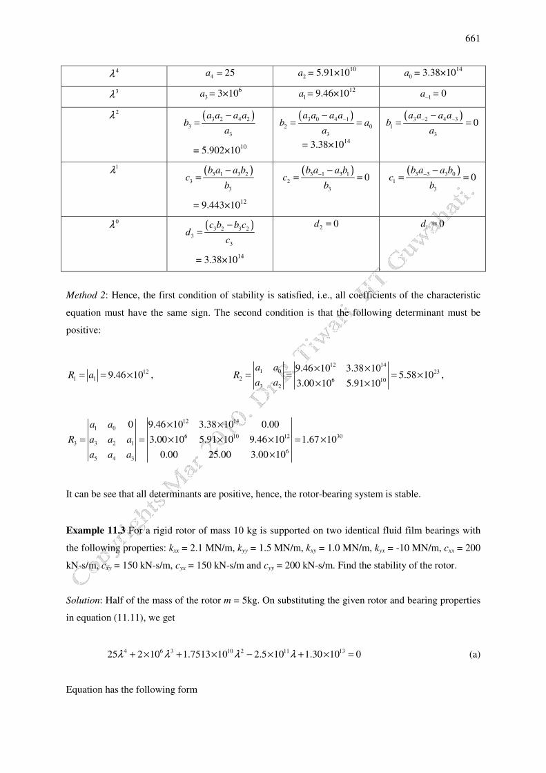
the system. For stable condition with unbalance in the system the path of the journal (journal orbit) for

a momentary disturbance will settle down to an elliptical shape (or an orbit with a fixed shape) after

sufficient iterations (Figure 11.4a).

(a) Stable (b) Unstable

Fig. 11.4 Journal center path due to perturbation

For no unbalance in the system it should converge to a point. For unstable system whirl orbit will not

be on ellipse (or an orbit with a fixed shape) but the whirl amplitude will increase with time (Figure

11.4b), indicating subsequent destruction of the bearing and then the rotor system itself.

For multi-DOF rotor-bearing systems the stability analysis will also be similar to what discussed here,

i.e., (i) Routh – Herwitz criteria, (ii) eigen value analysis, and (iii) plotting of the orbit for momentary

disturbances. However, last two methods are more practical to implement.

11.4 Resonant Whip

When the shaft rotates at about twice the speed associated with the first critical speed of the system,

the oil whirl takes place at the half the rotational speed and hence equal to the first critical speed of the

system. This condition is called oil-whip. In these circumstances very severe unstable vibrations

indeed are introduced and the situation is the most undesirable. The effect of vibration associated with

oil whirl combines with a system critical speed to produce most excessive vibration. It is the cross-

665

coupled stiffness (kxy and kyx) of the fluid-film bearing which destabilizes the rotor-bearing system.

Although the damping in fluid-film bearings is high, it is not sufficient to suppress the oil whip at high

rotor speeds. In this situation bearings will be in unstable operating regime. Muszynska (1986)

explained the difference between the oil whip and oil whirl. The oil whirl is stable and its frequency is

always around half the rotor speed, whereas, the oil whip is unstable and it has fixed frequency of

twice the first critical speed of the system. Oil whirl and oil whirl are nonlinear vibration phenomena

and cannot be described as such by linear vibration analysis.

As shown in Figure 11.5 in zone A: No oil whirl is present and only significant vibration is associated

with the unbalance at 1× shaft rotation. In zone B: Oil whirl is present at ω×21 and critical speed

effect. In zone C: When the oil-whirl vibration corresponds to system resonant frequency and one

having extremely high amplitude. In zone D: Oil-whirl subsides and only out of balance response will

be present.

Figure 11.5 Journal vibration frequency spectra showing the oil-whirl and the oil-whip

Example 13.3 A rigid rotor of mass 10 kg is supported by two identical fluid film bearings with the

following properties: kxx = 20 MN/m, cxx = 2 kN-s/m. Obtain the frequency of oil whip.

Solution: The undamped natural frequency of the rotor-bearing system, with mass of m and effective

support stiffness of 2kxx, is

666

62 2 20 10

200010

xxnf

km

ω × ×= = = rad/s

Hence, the damped natural frequency is given as

2 21 2000 1 0.1 1989.98d

nf nfω ω ζ= − = − = rad/s

with 32 2 2 10

0.12 2 10 2000nf

cm

ζω

× ×= = =× ×

Hence, the oil whip will take place when the rotor is at resonance and the frequency of the oil whip

will be 995 rad/s (i.e., at the half of the resonance frequency).

11.5 Internal Friction

Engineering materials show some resistance to their deformation which is a function of their rate of

deformation. Such a material property may be represented by damping force when modeling the

material behaviour. The damping effect also produced by the friction forces between mating

components of a shaft when the shaft deflects and the components move relative to each other. These

forces are particularly significant where interference fit components are present (Fig. 11.6).

Figure 11.6 A shaft-bearing system with an interference fit

When shaft elongates at the location of the interface AA (Figure 11.6b), the friction force opposes the

shaft deformation, these forces provide a hysteretic damping effect. Similar effect will be there at

interface BB. This kind of damping can be modeled as force proportional to the rate of shaft

deformation, as compared to the viscous damping which is proportional to absolute velocity of the

rotor.

667

Figure 11.7 The rotor motion with respect to the fixed and rotating frame of references

From Figure 11.7, we have

CF DOx= = , CD FOy= = CG EOξ= = ; CE GOη= = ;

Noting above expressions, we have

DO HO DH OE cos CE sin cos sinx t t t tω ω ξ ω η ω= = − = − = − (11.19)

and

CD ID CI EH CI OE sin CE cos sin cosy t t t tω ω ξ ω η ω= = + = + = + = + (11.20)

Let

js x y= + (11.21)

and

jζ ξ η= + (11.22)

On substituting equations (11.19) and (11.20) into equation (11.21), we get

j j j

j ( cos sin ) j( sin cos )

(cos jsin ) ( sin jcos ) j ( j )t t t

s x y t t t t

t t t t e e eω ω ω

ξ ω η ω ξ ω η ω

ξ ω ω η ω ω ξ η ξ η

= + = − + +

= + + − + = + = +

Noting, equation (11.22), we get

j ts e ωζ= (11.23)

668

Equation (11.23) is the transformation between stationary and rotating coordinate systems, where ω

is the spin speed of the shaft. On taking the first and second differentiations of equation (11.23) gives

j j j( j ) ( j )t t ts e e eω ω ωζ ζ ω ζ ωζ= + = +� �� (11.24)

and j j j 2 j 2 j( j ) ( j ) ( j ) ( 2 j )t t t t ts e e e e eω ω ω ω ωζ ζ ω ζ ω ζ ω ζ ωζ ω ζ= + + + = + −�� � � �� ��� (11.25)

Equations of motion of the Jeffcott rotor can be written as

0Vmx c x kx+ + =�� � and 0Vmy c y ky+ + =�� � (11.26)

where Vc is the viscous damping. On combining equation (11.26), noting equation (11.21), we get

0Vms c s ks+ + =�� � (11.27)

On substituting equations (11.23)-(11.25) into equation (11.27), we get

2( 2 j ) ( j ) 0Vm c kζ ωζ ω ζ ζ ωζ ζ+ − + + + =�� � � (11.28)

Separating the real and imaginary parts of equation (11.28), we get

2( 2 ) ( ) 0Vm c kξ ωη ω ξ ξ ωη ξ− − + − + =�� �� (11.29)

and 2( 2 ) ( ) 0Vm c kη ωξ ω η η ωξ η+ − + + + =��� � (11.30)

Fig. 11.8 The hysteretic damping force in a rotor in the rotating coordinate system

669

Now with the hysteretic damping, Hc , also (Fig. 11.8), hysteretic damping forces act along ξ and η

directions with values of Hc ξ� and Hc η� , respectively. Hence, equations (11.29) and (11.30) can be

modified as

2( 2 ) ( ) 0H Vm c c kξ ωη ω ξ ξ ξ ωη ξ− − + + − + =�� � �� (11.31)

and 2( 2 ) ( ) 0H Vm c c kη ωξ ω η η η ωξ η+ − + + + + =��� � � (11.32)

Again combining equations (11.31) and (11.32), we get

2( 2 j ) ( j ) 0H Vm c c kζ ωζ ω ζ ζ ζ ωζ ζ+ − + + + + =�� � � �

or 2(2 j ) ( j ) 0H V Vm m c c k m cζ ωζ ζ ω ω ζ+ + + + − + =�� � � (11.33)

where ζ is the complex displacement and for the asynchronous whirl can be defined as

0j0

te λζ ζ= (11.34)

which gives

0j0 0j te λζ ζ λ=� and 0j2

0 0te λζ ζ λ= −�� (11.35)

where 0ζ is the complex whirl amplitude in rotating coordinate systems, 0λ is defined as the relative

whirl frequency (or the whirl frequency in the rotating coordinate system ξ-η) of the rotor ( 0λ λ ω= −

) and � is the whirl frequency in the stationary coordinate system x-y. It should be noted that for

0 0λ = , we have the synchronous whirl condition ( λ ω= ) and for such case there will not be any

hysteretic damping, since the shaft whirls as rigid body in the bend configuration. On substituting

equations (11.34) and (11.35) in equation (11.33), it gives

( ){ } ( ){ }2 20 02 j j 0H V Vm m c c k m cλ ω λ ω ω− + − + + + − + = (11.36)

A general form of equation (11.36), a quadratic polynomial with complex coefficients, is

670

2

0 0 0 1 1 0 2 2( j ) ( j ) ( j ) 0a b a b a bλ λ+ + + + + = (11.37)

For which the Routh-Hurwitz stability criteria are (which is of different form as described previously

in Section 11.2)

010

10 >−bb

aa and 0

00

00

210

210

210

210

>

bbb

aaa

bbb

aaa

(11.38)

as the conditions for the imaginary part of 0λ to be negative (that is, for the amplitude of ζ to

decrease with time). On comparing equations (11.36) and (11.37), we get

0a m= − , 0 0b = , 1 2a mω= − , 1 H Vb c c= + , 22a k mω= − , 2 Vb c ω= (11.39)

From the first condition of equation (11.38), we have

20

0 H V

m m

c c

ω− −− >

+ ( ) 0H Vm c c� + > ( ) 0H Vc c� + > (11.40)

From the second condition of equation (11.38), we have

2

2

2 00 0

00 20 0

H V V

H V V

m m k m

c c cm m k m

c c c

ω ωωω ω

ω

− − −+

>− − −

+

(11.41)

which can be expanded as

2

02 0

0

H V V

H V V

c c c

m m m k m

c c c

ωω ω

ω

+− − − − >

+

or

( )2 02

( )( ) 0VH V

H V VH V V

cm k mm c c m m

c c cc c c

ωω ωωω

− −− + − − − >

++

671

or

( ) ( )( ){ }2 2 2 2 22 0H V V H V Vm c c c m c c k m m cω ω ω− + − − + − − >

or ( )( )2 2 2 2 2 2 2 2 22 2 2 0H V V H V H V nf Vc c c c c c c cω ω ω ω ω+ + + + − − > with 2 /nf k mω =

or

( ) ( )2 2 2 2 2 0H V nf H Vc c c cω ω+ − + >

or

2

2 2

2

2

1

1

V

Hnf

V

H

cc

cc

ω ω

� �+� �

� �<� �

+� �� �

(11.42)

In general, 2 2/ 1V Hc c � , we have the following condition

1 Vnf

H

cc

ω ω� �

< +� �� �

(11.43)

To summarise conditions of the stability of the rotor system with the hysteretic damping from

equations (11.40) and (11.43), it can be written as

0H Vc c+ > and 1 Vnf

H

cc

ω ω� �

< +� �� �

(11.44)

with 2 /nf k mω = (11.45)

The second condition indicates that system is always stable, even in the presence of hysteretic

damping, below the critical speed nfω . For the present case, both Vc and Hc are assumed to be

positive. In presence of viscous damping, however, has the effect of raising the speed at which the

system becomes unstable, so that if sufficient viscous damping is designed into the system then the

instability threshold speed (i.e., the speed below which the rotor has always stable operation) due to

hysteretic damping can be raised beyond the normal operating speed range of the machine, however,

the shift would be marginal.

672

Example 11.3 For a Jeffcott rotor, with mass disc of 2 kg, and a shaft of diameter of 0.01 m and

length of 0.6 m. It is found that the ratio of the coefficients of viscous and hysteretic damping to be

0.2. For the shaft take 112.1 10E = × N/m2. Find the speed of the instability threshold.

Solution: The stiffness of the shaft is given as

11 10

43 3

48 48 2.1 10 4.909 102.29 10

0.6EI

kl

−× × × ×= = = × N/m

The natural frequency of the rotor system is given as

42.29 10107.03

2nf

km

ω ×= = = rad/s

Hence the speed of instability threshold from equation (11.44) is : 107.03×1.2 = 128.43 rad/s. It can

be observed that for the present case, from equation (11.42), we get 128.40 rad/s, which is very close

to the above approximate value.

Example 11.4 For a Jeffcott rotor, with mass disc of 2 kg, and a shaft of diameter of 0.01 m and

length of 0.6 m. It is found that the ratio of the coefficients of viscous and the hysteretic damping to

be 0.2. The viscous damping ratio in the system is 0.01. For the shaft take 112.1 10E = × N/m2. Plot the

response in time domain for some initial condition at following speeds (i) 0.2 nfω ω= (ii) 0.9 nfω ω=

(iii) 1.6 nfω ω= and (iv) 1.2 nfω ω= , where nfω is the undamped natural frequency.

Solution: From equation (11.33), the equation of motion of the rotor in rotating coordinate system

with the viscous and hysteretic dampings, we have

2( 2 j ) ( j ) 0H Vm c c kζ ωζ ω ζ ζ ζ ωζ ζ+ − + + + + =�� � � �

(a)

The transformation from the rotating to stationary coordinate systems is given as

- j tse ωζ = (b)

so that

( ) - jj ts s e ωζ ω= −� � and ( )2 - j2 j ts s s e ωζ ω ω= − −�� �� � (c)

673

On subsisting equations (b) and (c) in equation (a), we get

( )j 0H Vms c s s c s ksω+ − + + =�� � � (d)

On separating real and imaginary parts of equation (d), we get

( ) 0H V Hmx c c x kx c yω+ + + + =�� � (e)

and

( ) 0H V Hmy c c y ky c xω+ + + − =�� � (f)

It should be noted that equations (e) and (f) are linear coupled ordinary differential equations. For

obtaining the response both equations have to be integrated simultaneously by any direct numerically

integration technique. Typical vibration responses for some initial conditions have been generated at

following speeds (i) 0.2 nfω ω= (ii) 0.9 nfω ω= (iii) 1.6 nfω ω= and (iv) 1.2 nfω ω= and are shown in

Figs. 11.9-11.12, respectively. Figures contain free responses in time domain and its orbit plots (i.e.,

x-y plot). It can be seen that for the first three cases the system is stable (Figs. 11.9-11.11) and for

fourth case it is unstable (Fig. 11.12). It should be noted that for large oscillations linear theory would

cease to be valid and response then would be governed by nonlinear behaviour of the system to

prevent very large oscillations before failure.

Time (s)

Fig. 11.9 (a) The rotor free vibration response in time domain for 0.2 nfω ω=

Dis

plac

emen

t (m

m)

Fig. 11.9 (b) The rotor orbit response for a short time interval for

Fig 11.9 (c) The rotor orbit response for a long time interval for

Fig. 11.10 (a) The rotor free vibration response in time domain for

Dis

plac

emen

t (m

m)

Dis

plac

emen

t in

y-di

rect

ion

(mm

) D

ispl

acem

ent i

n y-

dire

ctio

n (m

m)

The rotor orbit response for a short time interval for ω ω=(S is the starting point)

The rotor orbit response for a long time interval for ω ω=

Time (s)

Fig. 11.10 (a) The rotor free vibration response in time domain for

Displacement in x-direction (mm)

Displacement in x-direction (mm)

674

0.2 nfω ω=

0.2 nfω ω=

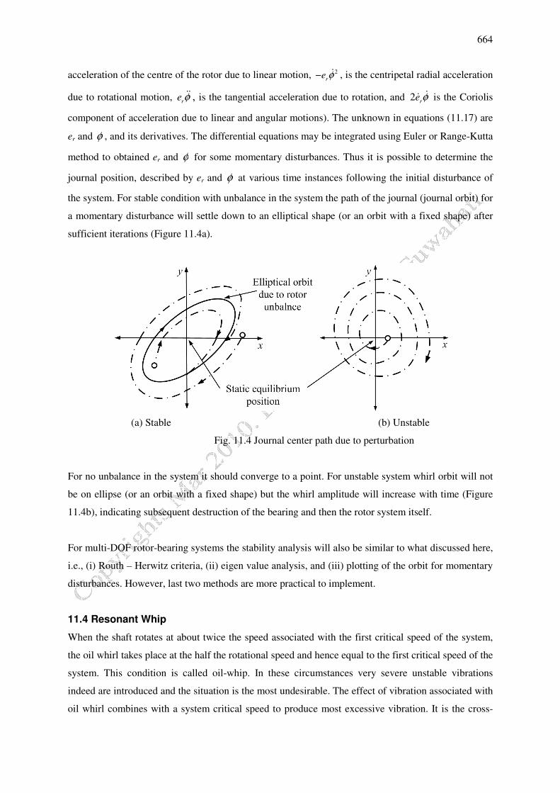
Fig. 11.10 (a) The rotor free vibration response in time domain for 0.9 nfω ω=

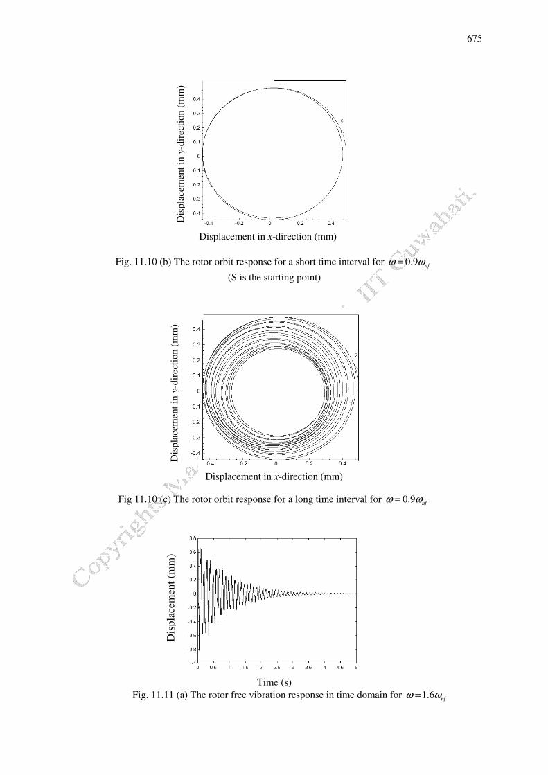
Fig. 11.10 (b) The rotor orbit response for a short time interval for

Fig 11.10 (c) The rotor orbit response for a long time interval for

Fig. 11.11 (a) The rotor free vibration response in time domain for

Dis

plac

emen

t (m

m)

Dis

plac

emen

t in

y-di

rect

ion

(mm

) D

ispl

acem

ent i

n y-

dire

ctio

n (m

m)

Fig. 11.10 (b) The rotor orbit response for a short time interval for ω ω(S is the starting point)

(c) The rotor orbit response for a long time interval for ω ω=

Time (s)

(a) The rotor free vibration response in time domain for

Displacement in x-direction (mm)

Displacement in x-direction (mm)

675

0.9 nfω ω=

0.9 nfω ω=

(a) The rotor free vibration response in time domain for 1.6 nfω ω=

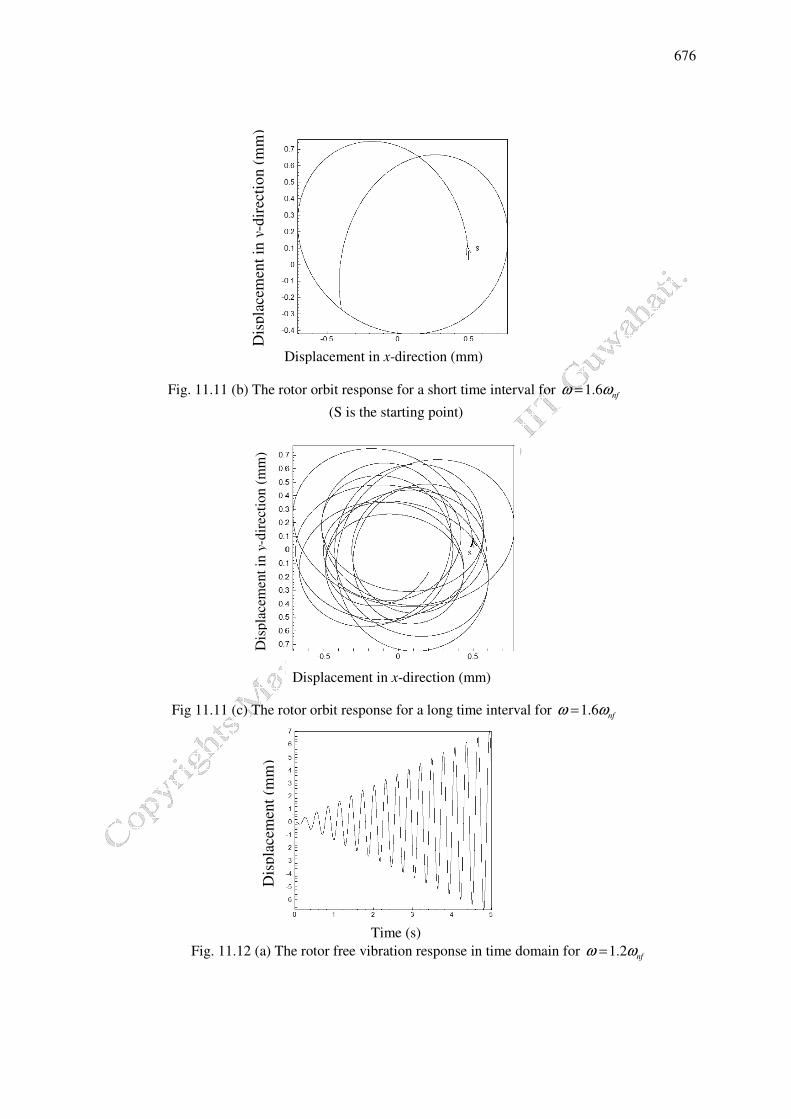
Fig. 11.11 (b) The rotor orbit response for a short time interval for

Fig 11.11 (c) The rotor orbit response for a long time interval for

Fig. 11.12 (a) The rotor free vibration response in time domain for

Dis

plac

emen

t (m

m)

Displacement in

Dis

plac

emen

t in

y-di

rect

ion

(mm

) D

ispl

acem

ent i

n y-

dire

ctio

n (m

m)

(b) The rotor orbit response for a short time interval for ω ω

(S is the starting point)

(c) The rotor orbit response for a long time interval for ω ω=

Time (s)

(a) The rotor free vibration response in time domain for

Displacement in x-direction (mm)

Displacement in x-direction (mm)

676

1.6 nfω ω=

1.6 nfω ω=

(a) The rotor free vibration response in time domain for 1.2 nfω ω=

677

Fig 11.12 (b) The rotor orbit response for a long time interval for 1.2 nfω ω=

11.6 Effect of Rotor Polar Asymmetry

In many machines the lateral stiffness of the rotor is different in two orthogonal directions. For

electrical motor or generator, the rotor (Figure 11.13) may have slots containing electrical windings

on some, but not all, parts of its surface.

Figure 11.13 A generator rotor

For such rotors the stiffness about x-axis will be less as compared to y-axis (i.e. the shaft deforms

more when x-axis is horizontal as against when y-axis is horizontal, due to gravity load). In some case

to make the stiffness in two directions closer, stiffness-compensating slots in pole face are made. But

in several cases it cannot be assured the same stiffness in all transverse directions of the shaft.

Displacement in x-direction (mm)

Dis

plac

emen

t in

y-di

rect

ion

(mm

)

678

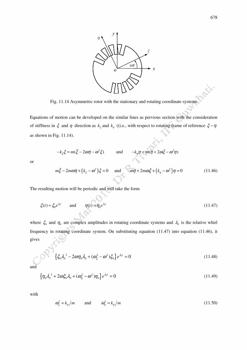
Fig. 11.14 Asymmetric rotor with the stationary and rotating coordinate systems

Equations of motion can be developed on the similar lines as pervious section with the consideration

of stiffness in ξ and η direction as kξ and kη ((i.e., with respect to rotating frame of reference ξ η−

as shown in Fig. 11.14).

2( 2 )k mξξ ξ ωη ω ξ− = − −�� � and 2( 2 )k mηη η ωξ ω η− = + −���

or

( )22 0m m kξξ ωη ω ξ− + − =�� � and ( )22 0m m kηη ωξ ω η+ + − =���

(11.46)

The resulting motion will be periodic and will take the form

00( ) tt eλξ ξ= and 0

0( ) tt eλη η= (11.47)

where 0ξ and 0η are complex amplitudes in rotating coordinate systems and 0λ is the relative whirl

frequency in rotating coordinate system. On substituting equation (11.47) into equation (11.46), it

gives

{ } 02 2 20 0 0 0 02 ( ) 0teλ

ξξ λ ωη λ ω ω ξ− + − = (11.48)

and

{ } 02 2 20 0 0 0 02 ( ) 0teλ

ηη λ ωξ λ ω ω η+ + − = (11.49)

with 2 k mξ ηω = and 2 k mη ηω = (11.50)

679

Equations (11.48) and (11.49) can be combined in a matrix form as

[ ]{ } {0}A X = (11.51)

with

2 2 20 0

2 2 20 0

( ) ( 2 )[ ]

2 ( )A ξ

η

λ ω ω ωλωλ λ ω ω

+ − −= � �+ −� � �

and { } 0

0

Xξη� �

= � �� �

The non-trivial solution of equation (11.51) is given by

4 2 2 2 2 2 2 2 20 0( 2 ) ( )( ) 0ξ η ξ ηλ ω ω ω λ ω ω ω ω+ + + + − − = (11.52)

The above equation can be solved to obtain the roots of �0 for various running speeds ω . Roots will

be in general complex. The real part of 0λ is if negative then the system is stable and if positive the

system is unstable. As discussed previously that for a negative value of the real part of 0λ , ξ (as well

as η ) decreases exponentially, and is given as

( )( ) cos sintt e A t B tαξ β β= + with 0 iλ α β= ± (11.53)

Alternatively stability may be investigated using the Routh-Hurwitz criteria for a polynomial of 4th

degree in 0λ , i.e., equation (11.13) (or quadratic in 20λ ). With either approach it is found that there is

a potential region of instability defined by (all the coefficients of the characteristic polynomial must

be of the same sign)

2 2 2 2( )( ) 0ξ ηω ω ω ω− − < for instability

which gives

ξ ηω ω ω< < for ξ ηω ω< (11.54)

In practice, there may be sufficient damping in the system to inhibit unstable vibration. The previous

analysis is based upon the assumption that the shaft vibration frequency ω corresponds to the

machine running speed (unbalance). This is a satisfactory assumption since in most cases the

predominant vibration frequency component is that associated with machine unbalance. However, in

the case of rotors with stiffness polar asymmetry, which are mounted, horizontally there is a

component of vibration frequency at twice machine running speed.

680

Figure 11.15 A rotor with asymmetry due to gravity load (a) less sag (b) more sag

The second moment of area about x-x in case (a) will be greater than for case (b) in Figure 11.15. For

this reason there will be greater sag of the rotor due to gravity for the latter rotor position as compared

with the former. Since the major and minor axes of the rotor section change orientation twice per

revolution, there will be a strong rotor vibration frequency component at twice the machine running

speed. For this reason there will be an unstable machine operating frequency range, for the

horizontally mounted rotor, defined by

vξ ηω ω< < or 2ξ ηω ω ω< < (11.55)

This can be arrived using the previous analysis with excitation frequency as in the previous case it

was v ω= due to unbalance only.

Example 11.4 An elliptical shaft with the length of 1 m, and the major and minor axes of 0.01 m and

0.009 m, respectively. The shaft carries a disc of mass 2 kg at the mid-span. For the steel shaft take 112.1 10E = × N/m2. Find the zones of the instability in the rotor system due to asymmetry of the shaft

cross-section.

Solution: The stiffness of the shaft in two principal directions are given as

11 8

53 3

48 48 2.1 10 7.952 108.02 10

1.0

EIk

lξ

ξ

−× × × ×= = = × N/m

with 2 2

80.005 0.00457.952 10

4 4ab

Iξπ π −× ×= = = × m4

and

681

11 85

3 3

48 48 2.1 10 8.836 108.91 10

0.6

EIk

lη

η

−× × × ×= = = × N/m

with 2 2

80.0045 0.0058.836 10

4 4ba

Iηπ π −× ×= = = × m4

Now, we have

58.02 10633.25

2

k

mξ

ξω ×= = = rad/s

and

58.91 10667.46

2

k

mη

ηω ×= = = rad/s

Hence, the rotor will be unstable in speed range 633.25 rad/s to 667.46 rad/s and in speed range of

316.67 to 333.73 rad/s.

11.7 An Asymmetric Rotor with Uniformly Distributed Mass

Let us consider a rotor as shown in Figure 11.16 with uniform distribution of mass. It could be

assumed as a large number of thin discs uniformly distributed along the shaft with an infinite number

of discs as the limiting case (Tondl, 1965).

Figure 11.16 A rotor with distributed mass property.

Let E be the modulus of elasticity of the shaft material, I1 and I2 are the principal area moments of

inertia of the shaft section, 22mk is the polar mass moment of inertia per unit length of the shaft

element (e.g., thin disc) with respect to axis of rotation, 2mk is the diametral mass moment of inertia

per unit length of the shaft element (e.g., thin disc) with respect to diametral axis, m is the mass per

unit length of shaft, k is the radius of gyration of the shaft element, ω is the angular velocity of the

shaft, xϕ and yϕ are the angular displacements about the x and y axes, respectively; and these are

chosen positive in accordance with right hand axis convection as shown in Figures 11.17. Let us first

682

derive equations of motion for 1 2I I= , then asymmetry of the shaft cross-section would be

introduced subsequently.

Figure 11.17 A rotor element

Figure 11.18 Positive directions of slopes and angular displacements (left) z-x plane (right) y-z plane

Equations of Motion: The angular displacement of the shaft element (denoted by xϕ and yϕ ) are given

by (see Figure 11.18)

( , )x

y z tz

ϕ ∂= −∂

and ( , )

y

x z tz

φ ∂=∂

(11.56)

where x and y are linear displacements. It should be noted that the positive direction of angular

displacement, xϕ , is opposite to the positive slope, dy/dz, direction; and the positive direction of

angular displacement, yϕ , is same to the positive slope, dx/dz, direction. So that the angular velocity

and acceleration can be written as

683

2

x

yz t

ϕ ∂= −∂ ∂

� and 2

y

xz t

ϕ ∂=∂ ∂

� (11.57)

and 3

2x

yz t

ϕ ∂= −∂ ∂

�� and 3

2y

xz t

ϕ ∂=∂ ∂

�� (11.58)

(a) A free-body diagram of the shaft element in z-x plane

(b) A free-body diagram of the shaft element in y-z plane

Figure 11.19 Gyroscopic and inertia moments on the shaft element (a) z-x and (b) y-z planes

Moment due to inertia forces of elements (taking moments in the y-z and z-x planes, and respective

directions positive in directions of xϕ and yϕ ) are given as (see Figure 11.19)

0yzx g d yM M I ϕ− − − =�� (11.59)

and

684

0xzy g d xM M I ϕ− + − =�� (11.60)

with gyroscopic moments (inertia moment) to the rotors are given as

yg P xM I ωϕ= − � and xg P yM I ωϕ= − � (11.61)

where zxM and zxM are moments which are applied to the rotor (disc) by the shaft. It should be noted

that in plane z-x the change in angular momentum over the time interval considered is P xI ωϕ and so

the gyroscopic couple which must be applied to produce this change, equal to the rate of change of

angular momentum, is given by P xI ωϕ� . In Figure 11.19(a) the gyroscopic couple applied to the shaft

through the rotor, P xI ωϕ� , must act about y-axis corresponding to the orientation of the vector

( )pI ω∆ in y-z plane (i.e., in the negative y-axis direction). Hence, the rotor will get a reactive couple,

yg P xM I ωϕ= − � . Similarly, in the plane y-z the change in angular momentum over the time interval

considered is P yI ωϕ and so the gyroscopic couple which must be applied to produce this change

equal to the rate of change of angular momentum, is given by P yI ωϕ� . In Figure 11.19(a) the

gyroscopic couple applied to the rotor , P yI ωϕ� , must act about x-axis corresponding to the orientation

of the vector ( )pI ω∆ in z-x plane (i.e., in the positive x-axis direction). Hence, the rotor will get a

reactive couple, xg P yM I ωϕ= − � . Equations (11.59) and (11.60), can be written as

zx d y P xM I Iϕ ωϕ= − +�� � (11.62)

and

zy d x P yM I Iϕ ωϕ= − −�� � (11.63)

For the shaft element (i.e., thin disc) we have, 2dI mk dz= and 22 2p dI I mk dz= = ; and noting

equations (11.57) and (11.58), from equations (11.59) and (11.60), we get

( ) ( )3 2 3 2

2 2 22 22 2zx

x y x yM mk dz mk dz mk dz

z t z t z t z tω ω� �∂ ∂ ∂ ∂= − − = − +� �∂ ∂ ∂ ∂ ∂ ∂ ∂ ∂� �

(11.64)

and

( ) ( )3 2 3 2

2 2 22 22 2yz

y x y xM mk dz mk dz mk dz

z t z t z t z tω ω� �∂ ∂ ∂ ∂= − + = − −� �∂ ∂ ∂ ∂ ∂ ∂ ∂ ∂� �

(11.65)

685

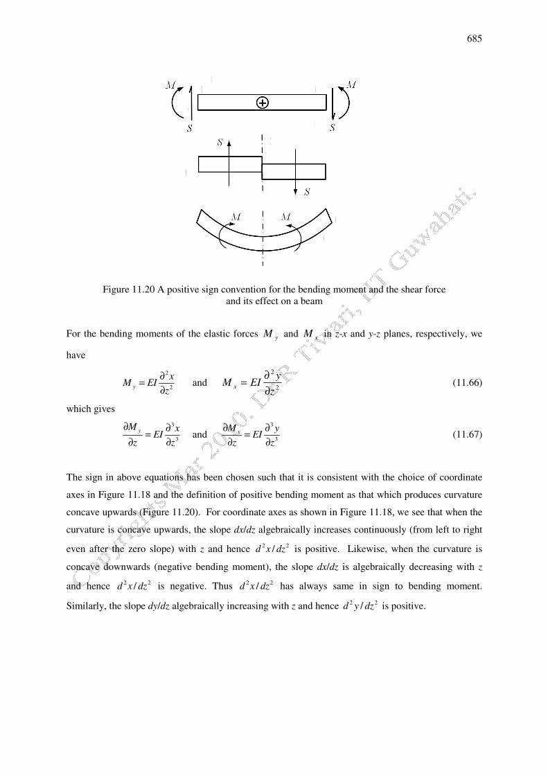
Figure 11.20 A positive sign convention for the bending moment and the shear force and its effect on a beam

For the bending moments of the elastic forces yM and xM in z-x and y-z planes, respectively, we

have

2

2y

xM EI

z∂=∂

and 2

2

zy

EIM x ∂∂= (11.66)

which gives

3

3yM x

EIz z

∂ ∂=∂ ∂

and 3

3xM y

EIz z

∂ ∂=∂ ∂

(11.67)

The sign in above equations has been chosen such that it is consistent with the choice of coordinate

axes in Figure 11.18 and the definition of positive bending moment as that which produces curvature

concave upwards (Figure 11.20). For coordinate axes as shown in Figure 11.18, we see that when the

curvature is concave upwards, the slope dx/dz algebraically increases continuously (from left to right

even after the zero slope) with z and hence 2 2/d x dz is positive. Likewise, when the curvature is

concave downwards (negative bending moment), the slope dx/dz is algebraically decreasing with z

and hence 2 2/d x dz is negative. Thus 2 2/d x dz has always same in sign to bending moment.

Similarly, the slope dy/dz algebraically increasing with z and hence 2 2/d y dz is positive.

686

(a) z-x plane (b) y-z plane

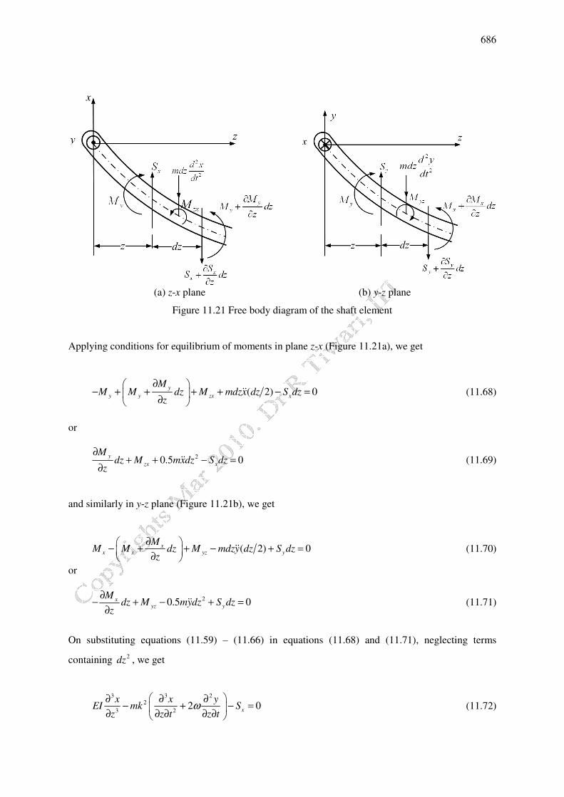
Figure 11.21 Free body diagram of the shaft element

Applying conditions for equilibrium of moments in plane z-x (Figure 11.21a), we get

( 2) 0yy y zx x

MM M dz M mdzx dz S dz

z

∂� �− + + + + − =� �∂� �

�� (11.68)

or

20.5 0yzx x

Mdz M mxdz S dz

z

∂+ + − =

∂�� (11.69)

and similarly in y-z plane (Figure 11.21b), we get

( 2) 0xx x yz y

MM M dz M mdzy dz S dz

z∂� �− + + − + =� �∂� �

�� (11.70)

or

20.5 0xyz y

Mdz M mydz S dz

z∂− + − + =∂

�� (11.71)

On substituting equations (11.59) – (11.66) in equations (11.68) and (11.71), neglecting terms

containing 2dz , we get

3 3 22

3 2 2 0x

x x yEI mk S

z z t z tω� �∂ ∂ ∂− + − =� �∂ ∂ ∂ ∂ ∂� �

(11.72)

687

and

3 3 22

3 2 2 0y

y y xEI mk S

z z t z tω� �∂ ∂ ∂− − − =� �∂ ∂ ∂ ∂ ∂� �

(11.73)

On differentiating equations (11.72) and (11.73) with respect to z, we get

4 4 3

24 2 2 22 0xSx x y

EI mkz z t z t z

ω� � ∂∂ ∂ ∂− + − =� �∂ ∂ ∂ ∂ ∂ ∂� � (11.74)

and

4 4 3

24 2 2 22 0ySy y x

EI mkz z t z t z

ω∂� �∂ ∂ ∂− − − =� �∂ ∂ ∂ ∂ ∂ ∂� �

(11.75)

From the condition for the equilibrium of forces acting on the element we have

2

2x

x x

S xS S dz mdz

z t∂ ∂� �− + =� �∂ ∂� �

or 2

2xS x

mz t

∂ ∂= −∂ ∂

(11.76)

Similarly, we have

2

2y

y y

S yS S m

z t

∂� � ∂− + = −� �∂ ∂� � or

2

2yS y

mz t

∂ ∂= −∂ ∂

(11.77)

On substituting equations (11.76) and (11.77) into equations (11.74) and (11.75), we get

4 4 3 22

4 2 2 2 22 0x x y x

EI mk mz z t z t t

ω� �∂ ∂ ∂ ∂− + + =� �∂ ∂ ∂ ∂ ∂ ∂� � (11.78)

and

4 4 3 22

4 2 2 2 22 0y y x y

EI mk mz z t z t t

ω� �∂ ∂ ∂ ∂− − + =� �∂ ∂ ∂ ∂ ∂ ∂� � (11.79)

Denoting js x y= + , equations (11.78) and (11.79) can be combined as

( )34 4 22

4 2 2 2 2

j( j ) ( j ) ( j )2 0

y xx y x y x yEI mk m

z z t z t tω

� �∂ −∂ + ∂ + ∂ +− + + =� �� �∂ ∂ ∂ ∂ ∂ ∂� � (11.80)

688

which can be written as

4 4 3 22

4 2 2 2 22j 0s s s s

EI mk mz z t z t t

ω� �∂ ∂ ∂ ∂− − + =� �∂ ∂ ∂ ∂ ∂ ∂� � (11.81)

Figure 11.22 The stationary and rotating coordinate systems

Let the complex displacement in the rotating coordinate system )( ηξ − as shown in Figure 11.22 be

defined as

( , ) ( , ) j ( , )z t z t z tζ ξ η= + (11.82)

The transformation from the stationary coordinate system (x-y) to the rotating coordinate system

)( ηξ − is given as

( , ) ( , ) j ts z t z t e ωζ= (11.83)

On differentiating equation (11.83) with respect to time, t, and space, z; we get

j( j ) ts e ωζ ωζ= +�� ; ( ) ( )2 2 2 jj j j 2 j ts e ωζ ωζ ωζ ω ζ ζ ωζ ω ζ= + + + = + −�� � � �� ��� (11.84)

and

j ts e ωζ′′′′ ′′′′= ; j( j ) ts e ωζ ωζ′′ ′′ ′′= +�� ; ( )2 j2 j ts e ωζ ωζ ω ζ′′ ′′ ′′ ′′= + −�� ��� (11.85)

Transforming equation (11.81) into the rotating co-ordinate system )( ηξ − by substituting equations

(11.83) and (11.84), we get

689

( ){ } ( )4

2 2 24 2j 2 j ( j ) 2 j 0EI mk m

zζ ζ ωζ ω ζ ω ζ ωζ ζ ωζ ω ζ∂ ′′ ′′ ′′ ′′ ′′− + − − + + + − =

∂�� � � �� � (11.86)

which can be simplified as

4 4 2 22 2

4 2 2 2 2 2j 0EI mk mz z t z t tζ ζ ζ ζ ζω ω ωζ� � � �∂ ∂ ∂ ∂ ∂− + + + − =� � � �∂ ∂ ∂ ∂ ∂ ∂� � � �

(11.87)

Separating the real and imaginary parts and introducing the unequal moments of inertia 1I and 2I ,

along ξ and η directions, respectively, we get

( )'''' 2 2 21 2 0EI

km

ξ ξ ω ξ ξ ωη ω ξ′′ ′′− + + − − =�� �� � (11.88)

and

( )'''' 2 2 22 2 0EI

km

η η ω η η ωξ ω η′′ ′′− + + + − =��� �� (11.89)

Boundary Conditions & Frequency Equation: For simply supported shaft corresponding boundary

conditions are

(0, ) ( , ) (0, ) ( , ) 0t L t t L tξ ξ η η= = = = for displacements (11.90)

and

(0, ) ( , ) (0, ) ( , ) 0t L t t L tξ ξ η η′′ ′′ ′′ ′′= = = = for bending moments (11.91)

Equations of motion (equations (11.88) and (11.89)) and boundary conditions (equations (11.90) and

(11.91)) then satisfy the following solution

0sin cosn z

A tLπξ λ= and 0sin sin

n zB t

Lπη λ= (11.92)

where A and B are constants, n = (1, 2, 3, …), L is the length of the shaft, λ is the natural frequency in

the stationary coordinate system (x, y, z) and ωλλ −=0 is the natural frequency in the rotating

coordinate system ),,( zηξ .

0 0sin sinn z

A tLπξ λ λ= −� , 0 0sin cos

n zB t

Lπη λ λ=�

690

20 0sin cos

n zA t

Lπξ λ λ= −�� , 2

0 0sin sinn z

B tLπη λ λ= −��

2

0sin cosn n z

A tL Lπ πξ λ� �′′ = − � �

� �,

2

0sin sinn n z

B tL Lπ πη λ� �′′ = − � �

� �

2

00sin cos

n n zA t

L Lπλ πξ λ� �′′ = � �

� ��� ,

20

0sin sinn n z

B tL Lπλ πη λ� �′′ = � �

� ���

4

0sin cosn n z

A tL Lπ πξ λ� �′′′′ = � �

� �,

4

0sin sinn n z

B tL Lπ πη λ� �′′′′ = � �

� � (11.93)

On substituting assumed solutions from equation (11.92) and its derivatives from equation (11.93) in

equations of motion (equations (11.88) and (11.89)), we get

( )24 2

2 2 2 2 2010 0 02 sin cos 0

nEI n n n zA k A k A A B A t

m L L L Lπλπ π πω λ ω λ ω λ

� �� �� �� � � �− − − + − − − =� �� �� � � �� �� � � �� �� �� �� � �

and

( ) ( )24 2

2 2 2 2 2020 0 02 sin sin 0

nEI n n n zB k B k B B A B t

m L L L Lπλπ π πω λ ω λ ω λ

� �� �� � � �− − − + − + − − =� �� �� � � �� � � �� � � �� �� �� � � which simplifies to

( ) ( ) ( )4 4 2 2

2 2 2 2 210 0 0 04 2 2 sin cos 0

EI n n n zk A B t

m L L Lπ π πλ ω λ ω ωλ λ

� �− − − + + − =� �� �

� � � (11.94)

and

( ) ( ) ( )4 4 2 2

2 2 2 2 220 0 0 04 22 sin sin 0

EI n n n zA k B t

m L L Lπ π πωλ λ ω λ ω λ

� �− + − − − + =� �� �

� � � (11.95)

For a non-trivial solution, the determinant of coefficients of linear homogeneous equations (11.94)

and (11.95) must be zero

691

( ) ( )

( ) ( )

4 4 2 22 2 2 2 21

0 0 04 2

4 4 2 22 2 2 2 22

0 0 04 2

20

2

EI n nk

m L LEI n n

km L L

π π λ ω λ ω ωλ

π πωλ λ ω λ ω

− − − + −=

− − − − + (11.96)

which gives the frequency equation as

( ) ( ) ( ) ( ) ( )4 4 2 2 4 4 2 2

22 2 2 2 2 2 2 2 2 22 10 0 0 0 04 2 4 2 2 0

EI EIn n n nk k

m L L m L Lπ π π πλ ω λ ω λ ω λ ω ωλ� �� �

− − − + − − − + − =� �� �� �� �

or

( ) ( ) ( ) ( )

( ) ( ) ( ) ( ) ( )

2 8 8 6 6 4 4 6 6 4 422 2 2 2 2 2 2 2 4 2 21 2 1 1 2

0 0 0 02 8 6 4 6 4

2 2 4 4 2 22 22 4 4 2 2 2 4 4 2 22

0 0 0 0 02 4 2 2 0

E I I EI EI EIn n n n nk k k

m L m L m L m L L

EIn n nk k

L m L L

π π π π πλ ω λ ω λ ω λ ω

π π πλ ω λ ω λ ω λ ω ωλ

− − − + − − + −

+ − − + + − + + − =

or

2 2 4 4 2 22 4 2 4

02 4 2

6 6 4 4 6 6 4 4 4 42 2 4 2 2 2 21 1 2 2

06 4 6 4 4

2 8 8 6 6 4 4 6 6 4 42 2 2 2 2 4 41 2 1 1 2

2 8 6 4 6 4

2 22

2

1

2 2 4

n n nk k k

L L L

EI EI EI EIn n n n nk k k

m L m L m L L m L

E I I EI EI EIn n n n nk k k

m L m L m L m L L

nk

L

π π π λ

π π π π πω ω ω λ

π π π π πω ω ω ω

π

� �+ + +� �

� �

� �+ − − − − − + −� �� �

� �+ + − + +� �� �

+ −4 4 2 2

4 2 2 4 424 2 0

EI n nk

m L Lπ πω ω ω ω� �

− − + =� �� �

or

4 4 2 24 2 4

04 2

6 6 4 4 4 42 4 2 2 21 2 1 2

06 4 4

2 8 8 6 6 4 4 2 2 4 42 2 2 2 4 4 4 41 2 1 2 1 2

2 8 6 4 2 4

2 1

( ) ( )2 2

( ) ( )2 0

n nk k

L L

E I I E I In n nk k

m L m L L

E I I E I I E I In n n n nk k k

m L m L m L L L

π π λ

π π π ω ω λ

π π π π πω ω ω ω ω

� �+ +� �

� �

� �+ ++ − − − −� �� �

� �� �+ +� �+ + − + − + + =� �� �� �� �� �

692

or

2 22 2 2 4 4 4 4 4 2 2 2 2 2 2

4 2 2 41 20 02 4 4 2 2

24 4 2 2 221 2

4 2

( )1 2 1 1 1

2

( ) 1

E I Ik n k n n k n k nL L m L L L

E I I E In k nm L L

π π π π πλ ω λ ω

π π ω

� � � � � � � �++ − + + + + −� �� � � � � � � �� � � � � � � � �

� �+− − +� �� �

8 81 22 8 0I n

m Lπ =

(11.97) Denoting

2

1 n

k na

Lπ� �+ =� �

� � and

2

1 n

k nb

Lπ� �− =� �

� � (11.98)

Whirl Natural Frequencies & Critical Speeds: Equation (11.97) gives the relative natural frequency as

4 4 4 4 42 2 1 2

0 4 4

2 24 4 4 4 4 4 4 8 82 2 2 4 21 2 1 2 1 2

4 4 4 2 8

( )1( ) 2 1

2 2

( ) ( )4 1 4

2

nn

n n n n

E I Ik n na

a L m L

E I I E I I E I Ik n n n na a b b

L m L m L m L

π πλ ω

π π π πω ω ω

� �� � +� �= + +� � �� �� �� � �� �

� � � �� � + +� �± + + − − +� � � �� �� �� � � �� �

(11.99)

To simplify equation (11.99), let us take terms within the square bracket separately and expand as

( )

2 2 24 4 4 4 4 4 4 4 8 84 2 21 2 1 2

4 4 4 2 8

24 4 8 82 2 4 2 2 21 2 1 2

4 2 8

( ) ( )4 1 2 1

2 4

( )4

n n

n n n n n

E I I E I Ik n k n n na a

L L m L m L

E I I E I In na b a b a

m L m L

π π π πω ω

π πω ω

� �� � � � + +� �� �+ + + +� �� � � �� �� �� � � �� � �

� �+− − +� �� �� � �

(11.100)

or

4 4 4 8 8 8 4 4 4 4 4 4 42 2 4 2 21 2 1 2

4 8 4 4 4

2 2 2 8 821 2 1 2

2 2 8

( ) ( )4 1 2 4 2 1

2

( )4

4

n n n n n

n

E I I E I Ik n k n k n n na b a a b

L L L m L m L

E I I E I I na

m m L

π π π π πω ω

π

� �� � � � + +� �+ + − + + +� � � �� �� �� � � �� �

� �++ −� �� �

(11.101)

693

From equation (11.98), we can have

2 2 2 2 2 2 4 4 4

2 2 41 1 1n n

k n k n k na b

L L Lπ π π� �� � � �

= + − = −� �� � � �� �� � � �

(11.102)

and 2 2 22 2 2 2 2 2 4 4 4 4 4 4 8 8 8

2 22 2 4 4 81 1 1 1 2n n

k n k n k n k n k na b

L L L L Lπ π π π π� � � � � �

= + − = − = − +� � � � � �� � � � � �

(11.103)

On substituting equations (11.102) and (11.103) into expression (11.101), we get

4 4 4 8 8 8 4 4 4 8 8 84

4 8 4 8

2 24 4 4 4 4 4 4 4 4 4 8 82 21 2 1 2 1 2

4 4 4 4 2 8

4 1 2 1 2

( ) ( ) ( )4 2 1 1 4

2 4n n n

k n k n k n k nL L L L

E I I E I I E I Ik n n n k n na a a

L m L m L L m L

π π π π ω

π π π π πω

� �+ + − + −� �

� �

� � � �� � � �+ + −� �+ + + − +� � � �� � � �� �� � � � � �� �

(11.104)

or

2 24 4 4 4 44 2 21 2 1 2

4 4 2 4 4

( ) ( )4 4 2

4n n

E I I E I Ik n na a

L mk m k Lπ πω ω

� �+ −� �+ +� � � �� �� � � � �

(11.105)

On substituting equation (11.105) into equation (11.99), we get

4 4 4 4 42 1 2

0 1,2,3,4 4 4

1/22 22 2 2 4 4

4 2 21 2 1 22 4 2 4 4

( )1( ) 1

2

2 ( ) ( ) 4

4

nn

n n

E I Ik n na

a L m L

E I I E I Ik n na a

L mk m k L

π πλ ω

π πω ω

�� � +�= ± + +�� ��� ��

� + − �± + + �� � ���

(11.106)

where n = (1, 2, 3, …). The absolute frequency is then

ωλλ += 4,3,2,10 )( (11.107)

Case I: 00 =λ so that ωλ = i.e. the whirl frequency is thus equal to the angular velocity, which

gives the synchronous forward precession or whirl. Equation (11.97) gives (for 00 =λ )

694

24 4 2 8 8

4 1 2 1 24 2 8 2

( ) 10

n n

E I I E I In nm L b m L b

π ω πω +− + = (11.108)

2 24 4 4 4 8 82 1 2 1 2 1 2

4 4 2 8 2

( ) ( )1 14

2 2n n n

E I I E I I E I In n nm L b b m L m L b

π π πω� �+ += ± −� �� �

( ){ }

[ ]

4 4 4 4 4 42 2 21 21 2 1 2 1 2 1 2 1 24 4 4

4 4

1 2 1 24

( ) 12 4 ( )

2 2 2

( )2

n n n

n

E I In n E E nI I I I I I I I I I

L mb L b m mb L

E nI I I I

mb l

π π π

π

+ = ± + + − = + ± − �

= + ± −

which gives

2 2 2 2* 1 1

2 2 2 2 2 2

/11 /n

n

EI EI mn nL b m L k n L

π πωπ

= =−

(11.109)

and

2 2** 2

2

1n

n

EInL b m

πω = (11.110)

where n = 1, 2, 3, …

For *nω and **

nω to be always real, we have

2 2 2

2 1k n

Lπ < or

Ln

kπ< (11.111)

Equation (11.111) will give the number of critical speeds, so finite number of synchronous forward

whirl critical speeds are possible.

Case II: For ωλ 20 −= ( hence, it gives λ ω= − that means the synchronous backward whirl or the

anti-synchronous precession. Thus, for ωλ 20 −= from equation (11.97), we get

695

4 4 4 4 4 4 44 2 2 2 4 21 2 1 2

4 4 4

2 8 81 22 8

( ) ( )(16 ) 2 1 (4 )

2

0

n n n n

E I I E I In k n na a b b

L m L m L

E I I nm L

π π πω ω ω ω ω

π

� � + +− + + + −� �� �� � �

+ =

(11.112)

which can be rearranged to

24 4 4 4 4 4 4 8 82 4 21 2 1 2 1 2

4 4 4 2 8

4 ( ) ( )16 8 1 0n n n n

E I I E I I E I In k n n na b a b

L m L m L m Lπ π π πω ω

� �� � � �+ +� �− + + + − − + =� � � �� �� �� � � �� �

(11.113) From equation (11.36) we can get critical speeds (�n

‡, �n‡‡) for anti-synchronous whirl, and critical

speeds of anti-synchronous whirl exit for all value of n. So there are infinite number of critical speeds

exits for the present case.

Case III: For moment of inertia forces and gyroscopic effect are negligible i.e. 0k = . The

characteristic equation (11.97) will reduce to

24 4 4 4 8 8

4 2 2 4 21 2 1 2 1 20 04 4 2 8

( ) ( )2 0

2E I I E I I E I In n n

m l m l m lπ π πλ ω λ ω ω� �+ +− + + − + =� �

� �

which can be rearranged to

4 4 4 4 4 44 2 2 2 21 2 1 2

0 04 4 4

( )2 0

2E I I EI EIn n n

m l m l m lπ π πλ ω λ ω ω� � � �� �+− + + − − =� � � �� �

� � � �� � (11.114)

For synchronous whirl 00 =λ , we get critical speeds, as

2 2* † 1

20n nk

EInl mπω ω

== = and

2 2** †† 2

20n nk

EInl mπω ω

== =

(11.115)

In this case we obtain an infinite number of critical speeds and an infinite number of intervals of

instability, † ††( , )n nω ω with 1,2,n = � . Equation (11.114) can be solved directly to get natural

frequency of the systems as (To be expanded)

696

2 24 4 2 2 4 42 21 2 1 2 1 2

1,2,3,4 4 2 2 4

( ) 2 ( ) ( )2 4

E I I E I I E I In n nm L L m m L

π π πλ ω ω ω� �+ + −� �= ± + ± +� �� �� �

2 2

2 2 2 2† ††

2 2 † †† † †† 212 ( ) ( )

2 4n n

n n n n

ω ωω ω ω ω ω ω ω� �+� � = ± + ± + + −� �� � �� �� �

(11.116)

where †nω and ††

nω are given as in equation (11.115). Equation (11.116) will give infinite number of

graphs of λ plotted as a function of ω (n = 1, 2, 3, …) and infinite number of intervals of instability.

Stability Analysis of Asymmetric Shaft with Gyroscopic Effects: Noting equation (11.98),

equation (11.97) can be written as

24 4 4 4 8 8

2 4 2 2 2 4 21 2 1 2 1 20 04 4 2 8

( ) ( )2 0

2n n n n n n

E I I E I I E I In n na a b a b b

m L m L m Lπ π πλ ω λ ω ω� �+ ++ + + − + =� �

� � (11.117)

which can be rearranged as

4 4 4 4 4 4 4 4

2 4 2 2 2 21 2 1 20 04 4 4 42 0

2n

n n n n n

a EI EI EI EIn n n na a b b b

m L m L m L m Lπ π π πλ ω λ ω ω

� �� � � �� �� �+ + + + − − =� �� � � �� �� �� � � �� �� �

(11.118) From equations (11.109) and (11.110), we get

24 4

* 14n n

EI nb

m Lπω = and

24 4

** 24n n

EI nb

m Lπω = (11.119)

Noting equation (11.119), equation (11.118) gives

( ){ } ( )( )2 2 2 22 4 * ** 2 2 2 * 2 **0 02 0n n n n n n na a bλ ω ω ω λ ω ω ω ω+ + + + − − = (11.120)

For the case of single disc with massless shaft or the case of polar asymmetry the characteristic

equation (equation (11.52)) is

4 2 2 2 2 2 2 2 20 0( 2 ) ( )( ) 0ξ η ξ ηλ ω ω ω λ ω ω ω ω+ + + + − − = (11.121)

and by the Routh-Hurwitz criteria the region of instability is defined by

2 2 2 2( )( ) 0ξ ηω ω ω ω− − < or ξ ηω ω ω< < (11.122)

697

Since we have k kξ η< and on comparing characteristic equation (11.120) and (11.121), on the similar

line we can obtain the condition of instability as

( )( )2 22 * 2 ** 0n nω ω ω ω− − < (11.123)

The above condition of instability is fulfilled only inside the interval ),( ***nn ωω (it is assumed here

that ***nn ωω > , i.e., 12 II > ). Thus we have finite number of intervals of instability. It may happen

that two intervals overlap, i.e. that they merge into a single interval of instability. The condition for

this to happen is, that

*

1**

+> nn ωω (11.124)

since n is finite so finite number of interval of instability.

Example 11.1: Consider a rotor system with the following rotor parameters: m = 0.981 kg, k = 3 cm,

1I = 5 cm4, 2I = 10 cm4, L = 100 cm and E = 112.1 10× N/m2. Obtain the instability plots up to third

mode and tabulate all the frequency range of instability. Obtain the critical speeds for (i) synchronous

whirl with gyroscopic effect (ii) anti-synchronous whirl with gyroscopic effect, and (iii) without

gyroscopic effect.

Solution: For the case when 0k ≠ , / ( ) 100 / ( 3) 10.6n L kπ π< = × = , so that n = 10. The gyroscopic

effect thus causes the intervals of instability to be reduced to a finite number (i.e., 10 for the present

case). Hence, we have 10 intervals of instability { * **( , ),n nω ω n = 1, 2, …, 10} as given in the second

and third columns in Table 11.4 for the synchronous whirl. No instability intervals overlap (or merge)

for the synchronous whirl. Figures 11.23 and 11.24 show variation of the forward whirl natural

frequency with the spin speed for the first mode and up to third modes, respectively. The shaded

frequency interval represent the instability zones, in Fig. 11.24 it can be seen that these zones are

distinct and no overlap is found in the instability zones up to third modes. Table 11.4 also lists

instability zones for anti-synchronous whirl in fourth and fifth columns. It can be seen that for the

anti-synchronous whirl the overlap of instability interval exist for different neighbouring modes.

Table 11.4 also lists first 10 instability zones for the case of no gyroscopic effect, i.e. 0k = and the

overlap of instability interval exist for different neighbouring modes.

698

Figure 11.23 Variation of whirl frequency with the spin speed for first mode

(Plot of equation (11.97) for n = 1)

-400 -300 -200 -100 0 100 200 300 4000

50

100

150

200

250

300

�1* =1

01.4

4

�1**

= 14

3.5

Spin frequency, rad/s

n=1 n=1

Whi

rl fr

eque

ncy,

rad/

s