CHAPTER 11Consumer Preferences and

Consumer Choice

2

What you will learn in this chapter:Why economists use indifference curves to

illustrate a person’s preferencesThe importance of the marginal rate of

substitution, the rate at which a consumer is just willing to substitute one good for anotherAn alternative way of finding a consumer’s

optimal consumption bundle using indifference curves and the budget lineHow the shape of indifference curves helps

determine whether goods are substitutes or complementsAn in-depth understanding of income and

substitution effects

3

Mapping the Utility Function

A utility function determines a consumer’s total utility given his or her consumption bundle.

Using indifference curves, which represent a consumer’s utility function, we will deepen our understanding of the trade-off involved when choosing the optimal consumption bundle and of how the optimal consumption bundle itself changes in response to changes in the prices of goods.

4

Ingrid’s Utility FunctionIngrid is indifferent between A and B: because A and B yield the same total utility level, Ingrid is equally well off with either bundle. Hence, a contour line that maps consumption bundles yielding the same amount of total utility is known as an indifference curve.

5

An Indifference Curve

An indifference curve is a line that shows all the consumption bundles that yield the same amount of total utility for an individual.

6

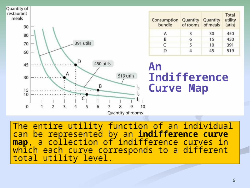
An Indifference Curve Map

The entire utility function of an individual can be represented by an indifference curve map, a collection of indifference curves in which each curve corresponds to a different total utility level.

7

Properties of Indifference Curves

All indifference curve maps share two general properties: indifference curves never cross, and the farther out an indifference curve is, the higher the total utility it indicates.

In addition, indifference curves for most goods, called ordinary goods, have two more properties: they are downward sloping and are convex (bowed-in toward the origin) as a result of diminishing marginal utility.

8

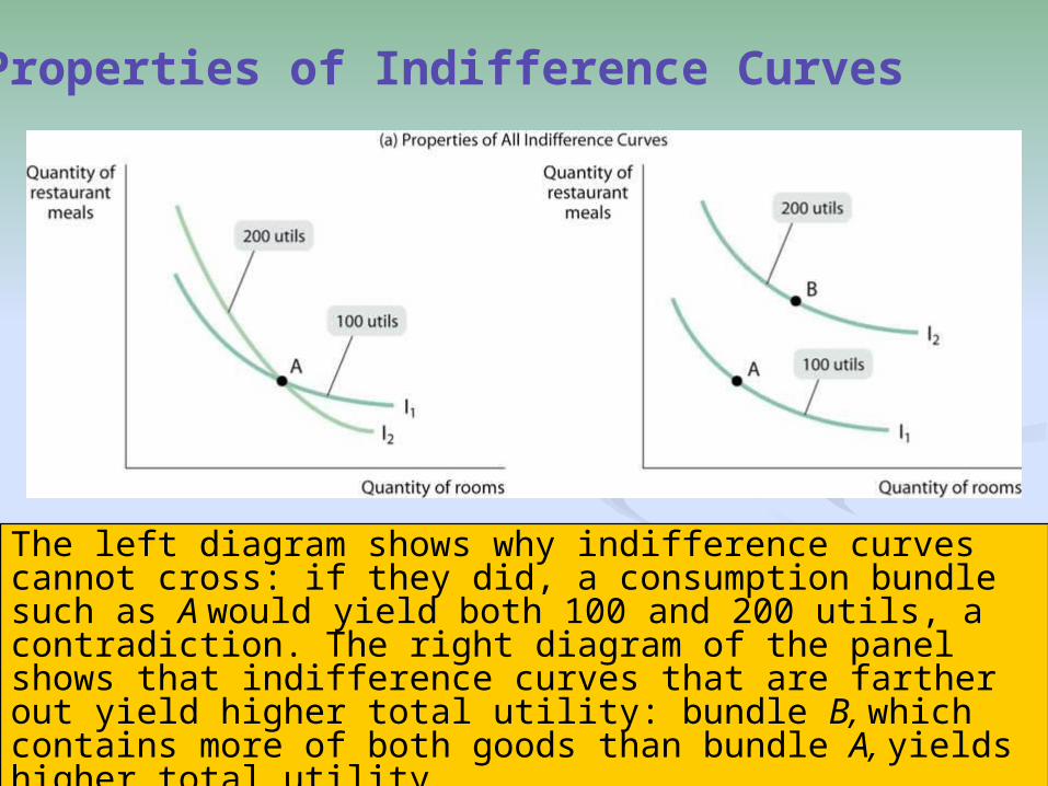
The left diagram shows why indifference curves cannot cross: if they did, a consumption bundle such as A would yield both 100 and 200 utils, a contradiction. The right diagram of the panel shows that indifference curves that are farther out yield higher total utility: bundle B, which contains more of both goods than bundle A, yields higher total utility.

Properties of Indifference Curves

9

Panel (b) depicts two additional properties of indifference curves for ordinary goods. The left diagram shows that indifference curves slope downward: as you move down the curve from bundle W to bundle Z, consumption of rooms increases. To keep total utility constant, this must be offset by a reduction in quantity of restaurant meals. The right diagram shows a convex-shaped indifference curve. The slope of the indifference curve gets flatter as you move down the curve to the right, a feature arising from diminishing marginal utility.

10

Indifference Curves and Consumer Choice

We will use indifference curve maps to find the utility-maximizing consumption bundle of a consumer given his/her budget constraint.

The optimal consumption bundle lies on the budget line, and the marginal utility per dollar is the same for every good in the bundle.

The first component of our approach is a new concept, the marginal rate of substitution.

11

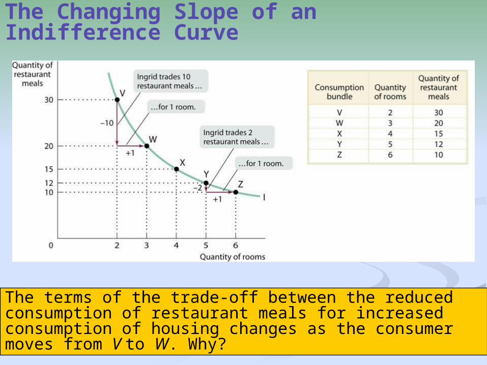
The Changing Slope of an Indifference Curve

The terms of the trade-off between the reduced consumption of restaurant meals for increased consumption of housing changes as the consumer moves from V to W. Why?

12

Two opposing effects on total utility:

Moving down the indifference curve—reducing restaurant meal consumption and increasing housing consumption—will produce two opposing effects on Ingrid’s total utility:Lower restaurant meal consumption will reduce her total utility, but higher housing consumption will raise her total utility. And since we are moving down the indifference curve, these two effects must exactly cancel out.

13

Two opposing effects on total utility (cont’d):

Hence, we can calculate the change in total utility generated by a change in the consumption bundle using the following equations:

Change in total utility arising from a change in consumption of restaurant meals = MUM× ∆QM

Change in total utility arising from a change in consumption of rooms = MUR × ∆QR

Along the indifference curve: −MUM × ∆QM = MUR × ∆QR

14

Marginal Rate of Substitution

The following equation would also hold along the indifference curve:

−MUR / MUM = ∆QM /∆QR

Economists have a special name for the ratio of the marginal utilities in the LHS of this equation and it is called the marginal rate of substitution, MRS.

15

Diminishing Marginal Rate of Substitution

The flattening of indifference curves as you slide down them to the right—which reflects the same logic as the principle of diminishing marginal utility—is known as the principle of diminishing marginal rate of substitution.

It says that an individual who consumes only a little bit of good A and a lot of good B will be willing to trade off a lot of B in return for one more unit of A; an individual who already consumes a lot of A and not much B will be less willing to make that trade-off.

16

The tangency condition between the indifference curve and the budget line holds when the indifference curve and the budget line just touch. This condition determines the optimal consumption bundle when the indifference curves have the typical convex shape.

Tangency Condition

17

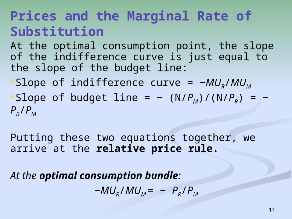
Prices and the Marginal Rate of SubstitutionAt the optimal consumption point, the slope of the indifference curve is just equal to the slope of the budget line:Slope of indifference curve = −MUR/MUM

Slope of budget line = − (N/PM)/(N/PR) = − PR/PM

Putting these two equations together, we arrive at the relative price rule.

At the optimal consumption bundle:−MUR/MUM = − PR/PM

18

Understanding the Relative Price Rule

At the optimal consumption bundle:

−MUR/MUM = − PR/PM

19

When we say that two consumers have different preferences, we mean that they have different utility functions.

This in turn means that they will have indifference curve maps with different shapes.

And those different maps will translate into different consumption choices, even among consumers with the same income who face the same prices.

Preferences and Choices

20

Differences in Preferences

Ingrid and Lars have different preferences. They choose different consumption bundles.

Both of them have an income of $2,400 and face prices of $30 per meal and $150 per room.

While Ingrid’s consumption choice is 8 rooms and 40 restaurant meals, Lars consumes fewer rooms and more restaurant meals even though he has the same budget line.

21

Case: “Rats and Rational Choice” A simple test for rationality:Economists have conducted experiments in which rats are presented with a “budget constraint”—a limited number of times per hour they can push either of two levers. One of the levers yields small cups of water; the other yields pellets of food. After the rat’s choices have been observed, the budget constraint is changed by varying the number of lever pushes required to get each good. Sure enough, the rats satisfy the rule for rational choice. If rats are rational, can people be far behind?

Economics in Action:

22

A Test for Rationality

A consumer has the budget line BL1 and chooses the bundle A. If that consumer is now given a new budget line—BL2, it would be irrational to choose a bundle such as B; the consumer could have afforded that bundle before but chose A instead. A rational consumer would always at least stay at A or choose a new bundle that was not affordable before, such as C. It’s difficult to test people in this way—but it works for rats!

23

What determines whether two goods are substitutes or complements?

It depends on the shape of a consumer’s indifference curves.

This relationship can be illustrated with two extreme cases: the cases of perfect substitutes and perfect complements.

Using Indifference Curves: Substitutes and Complements

24

Two goods are perfect substitutes if the marginal rate of substitution of one good in place of the other good is constant, regardless of how much of each an individual consumes.

Perfect Substitutes

25

When two goods are perfect substitutes, small price changes can lead to large changes in the consumption bundle. In panel (a), the relative price of chocolate chip cookies is slightly higher than the MRS of chocolate chip in place of peanut butter cookies; this is enough to induce Cokie to choose consumption bundle A, which consists entirely of peanut butter cookies. In panel (b), the relative price of chocolate chip cookies is slightly lower than MRS; this induces Cokie to choose bundle B, consisting entirely of chocolate chip cookies.

Consumer Choice Between Perfect Substitutes

26

Perfect Complements

Two goods are perfect complements when a consumer wants to consume the goods in the same ratio regardless of their relative price.

27

How would our consumption choice change if either the prices of goods or our income change?

First, let’s see the effects of a price increase illustrated in the following figure.

Then, we will consider the impact of a change in income.

Prices, Income, and Demand

28

Effects of a Price Increase on the Budget Line

An increase in the price of rooms, holding the price of restaurant meals constant, increases the relative price of rooms in terms of restaurant meals. As a result, Ingrid’s original budget line, BL1, rotates inward to BL2. Her maximum possible purchase of restaurant meals is unchanged, but her maximum possible purchase of rooms is reduced.

29

Responding to a Price Increase

Ingrid responds to the higher relative price of rooms by choosing a new consumption bundle with fewer rooms and more restaurant meals. Her new bundle, C, contains 1 room instead of 8 and 60 restaurant meals instead of 40.

30

Income and Consumption:Normal Goods

At a monthly income of $2,400, Ingrid chooses bundle A, consisting of 8 rooms and 40 restaurant meals. When relative price remains unchanged, a fall in income shifts her budget line inward to BL2. At a monthly income of $1,200, she chooses bundle B, consisting of 4 rooms and 20 restaurant meals. Since Ingrid’s consumption of both restaurant meals and rooms falls when her income falls, both goods are normal goods.

31

Income and Consumption: An Inferior Good

When Ingrid’s income falls from $2,400 to $1,200, her optimal consumption bundle changes from D to E. Her consumption of second-hand furniture increases, implying that second-hand furniture is an inferior good. In contrast, her consumption of restaurant meals falls, implying that restaurant meals are a normal good.

32

The change in a consumer’s optimal consumption bundle caused by a change in price can be decomposed into two effects: the substitution effect, due to the change in relative price, and the income effect, due to the change in purchasing power.

The substitution effect refers to the substitution of the good that is now relatively cheaper for the good that is now relatively more expensive, holding the utility level constant. It is represented by movement along the original indifference curve.

Income and Substitution Effects

33

When a price change alters a consumer’s purchasing power, the resulting change in consumption is the income effect. It is represented by a movement to a different indifference curve, keeping the relative price unchanged.For normal goods, the income and substitution effects work in the same direction; so their demand curves always slope downward. Although these effects work in opposite directions for inferior goods, their demand curves usually slope downward as well because the substitution effect is typically stronger than the income effect. The exception is the case of a Giffen good.

Income and Substitution Effects

34

Income and Substitution Effects

35

The End of Chapter 11

coming attraction:Chapter 12:

Factor Markets and the Distribution of

Income