Chapter 11 Aggregate Demand II - ACAD/WWW...
26
Chapter 11 Aggregate Demand II In this chapter, we learn • how to use the IS-LM model to analyze the effects of shocks, fiscal policy, and monetary policy • how to derive the aggregate demand curve from the IS-LM model
Transcript of Chapter 11 Aggregate Demand II - ACAD/WWW...
Chapter 11 Aggregate Demand II In this chapter, we learn • how to use the IS-LM model to analyze the
effects of shocks, fiscal policy, and monetary policy
• how to derive the aggregate demand curve from the IS-LM model
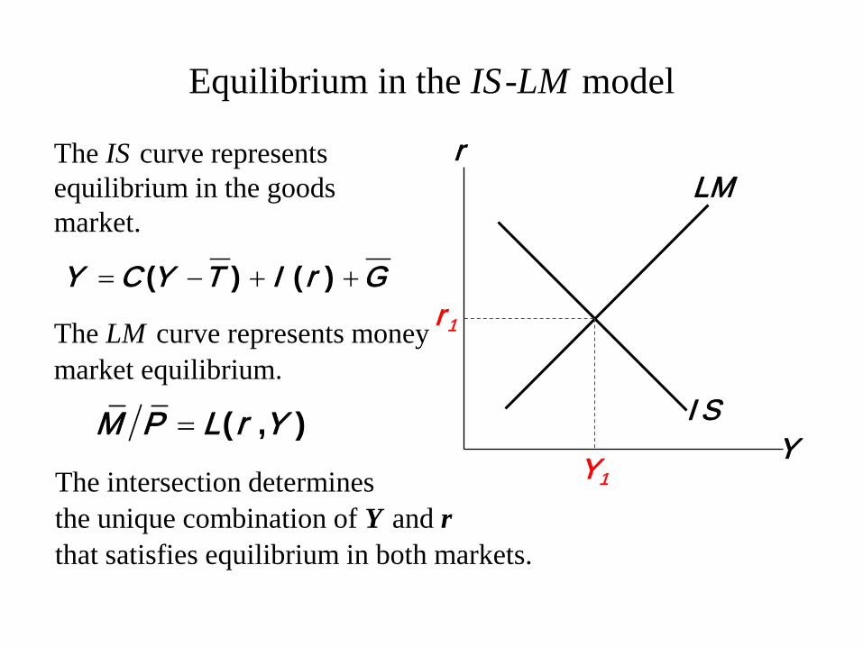
The intersection determines the unique combination of Y and r that satisfies equilibrium in both markets.
The LM curve represents money market equilibrium.
Equilibrium in the IS -LM model
The IS curve represents equilibrium in the goods market.
( ) ( )Y C Y T I r G= − + +
( , )M P L r Y= IS
Y
r LM
r1
Y1
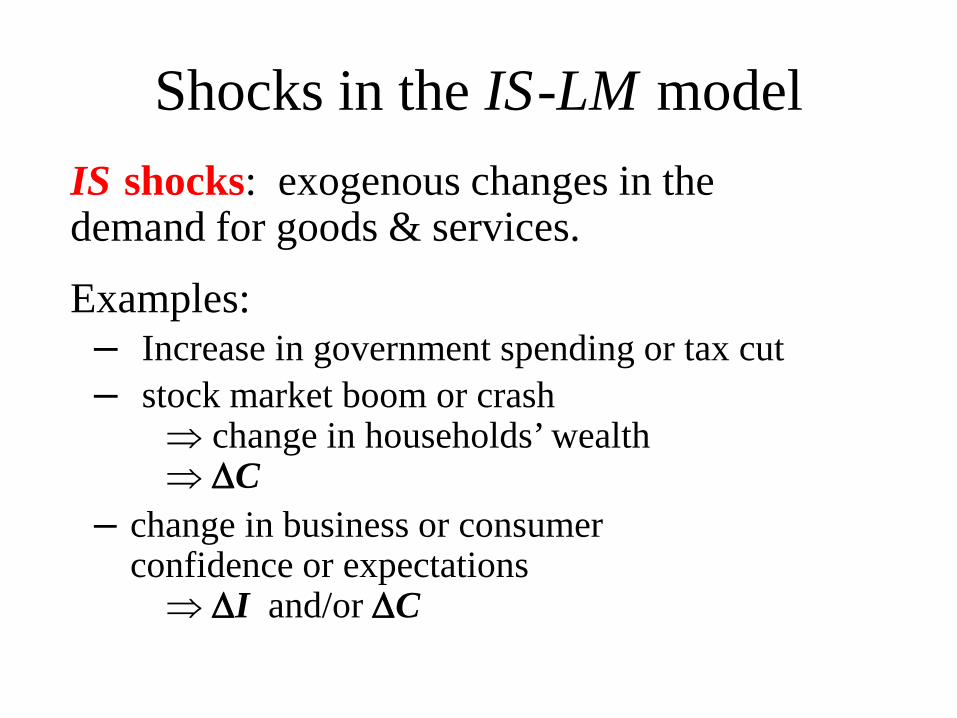
Shocks in the IS -LM model IS shocks: exogenous changes in the demand for goods & services.
Examples: – Increase in government spending or tax cut – stock market boom or crash
⇒ change in households’ wealth ⇒ ∆C
– change in business or consumer confidence or expectations ⇒ ∆I and/or ∆C
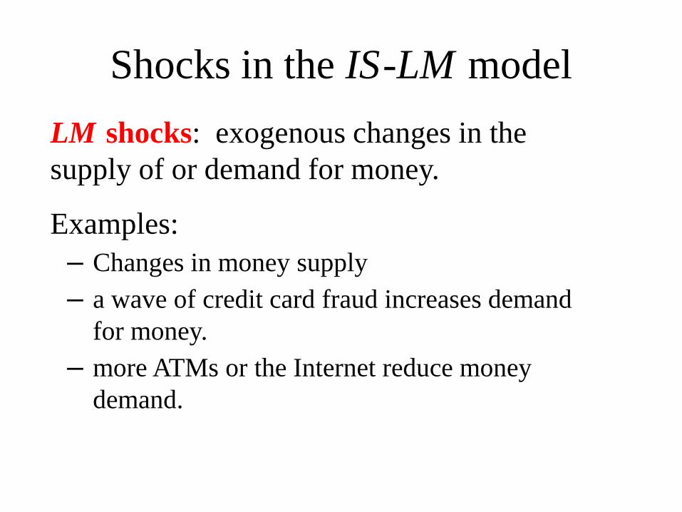
Shocks in the IS -LM model LM shocks: exogenous changes in the supply of or demand for money.
Examples: – Changes in money supply – a wave of credit card fraud increases demand
for money. – more ATMs or the Internet reduce money
demand.
causing output &
income to rise.
IS1
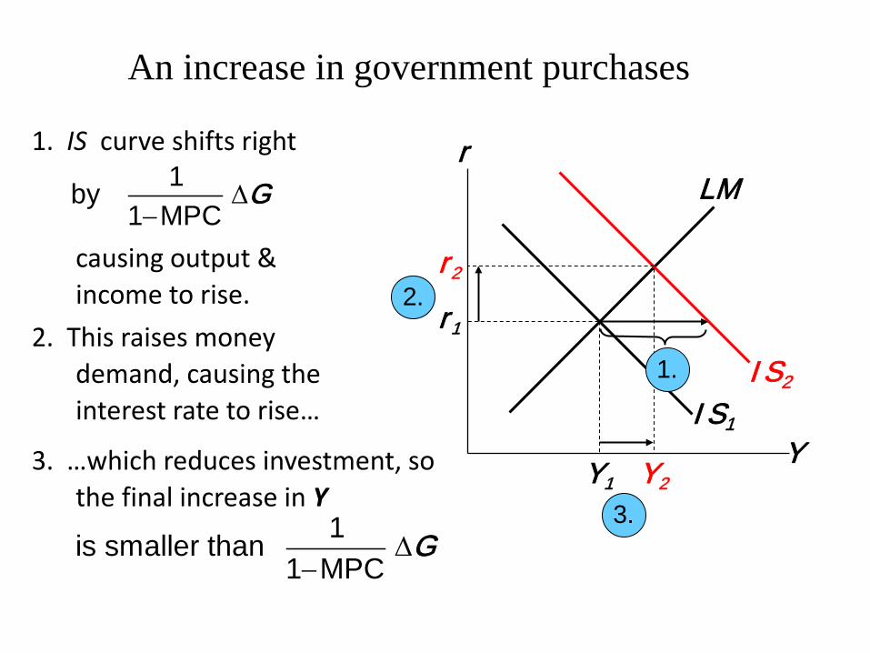
An increase in government purchases
1. IS curve shifts right
Y
r LM
r1
Y1
1by 1 MPC
G∆−
IS2
Y2
r2
1. 2. This raises money
demand, causing the interest rate to rise…
2.
3. …which reduces investment, so the final increase in Y
1is smaller than 1 MPC
G∆−
3.

IS1
1.
A tax cut
Y
r LM
r1
Y1
IS2
Y2
r2
Consumers save (1−MPC) of the tax cut, so the initial boost in spending is smaller for ∆T than for an equal ∆G… and the IS curve shifts by
MPC1 MPC
T−∆
−1.
2.
2. …so the effects on r and Y are smaller for ∆T than for an equal ∆G.
2.
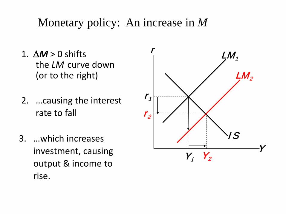
2. …causing the interest rate to fall
IS
Monetary policy: An increase in M
1. ∆M > 0 shifts the LM curve down (or to the right)
Y
r LM1
r1
Y1 Y2
r2
LM2
3. …which increases investment, causing output & income to rise.

Interaction between monetary & fiscal policy
• Model: Monetary & fiscal policy variables (M, G, and T ) are exogenous.
• Real world: Monetary policymakers may adjust M in response to changes in fiscal policy, or vice versa.
• Such interaction may alter the impact of the original policy change.

The Fed’s response to ∆G > 0
• Suppose Congress increases G. • Possible Fed responses:
1. hold M constant 2. hold r constant 3. hold Y constant
• In each case, the effects of the ∆G are different…
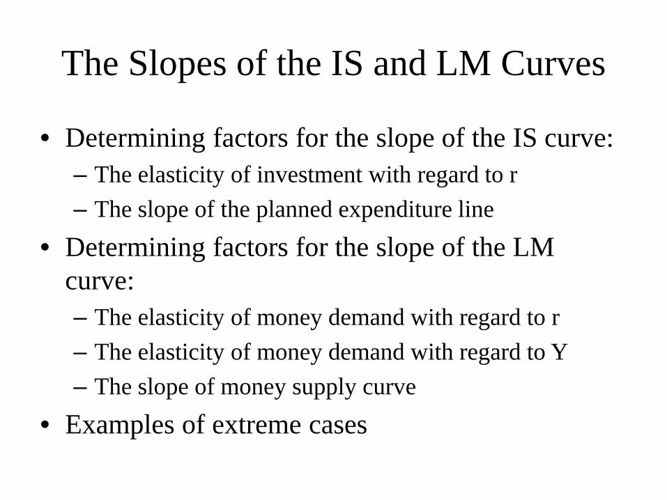
The Slopes of the IS and LM Curves
• Determining factors for the slope of the IS curve: – The elasticity of investment with regard to r – The slope of the planned expenditure line
• Determining factors for the slope of the LM curve: – The elasticity of money demand with regard to r – The elasticity of money demand with regard to Y – The slope of money supply curve
• Examples of extreme cases

CASE STUDY:
The U.S. recession of 2001
• During 2001, – 2.1 million jobs lost,
unemployment rose from 3.9% to 5.8%. – GDP growth slowed to 0.8%
(compared to 3.9% average annual growth during 1994-2000).

CASE STUDY:
The U.S. recession of 2001 Causes: 1) Stock market decline ⇒ ↓C
300
600
900
1200
1500
1995 1996 1997 1998 1999 2000 2001 2002 2003
Inde
x (1
942
= 10
0)
Standard & Poor’s 500

CASE STUDY:
The U.S. recession of 2001
Causes: 2) 9/11 – increased uncertainty – fall in consumer & business confidence – result: lower spending, IS curve shifted left
Causes: 3) Corporate accounting scandals – Enron, WorldCom, etc. – reduced stock prices, discouraged investment

CASE STUDY:
The U.S. recession of 2001
• Fiscal policy response: shifted IS curve right – tax cuts in 2001 and 2003 – spending increases
• airline industry bailout • NYC reconstruction • Afghanistan war
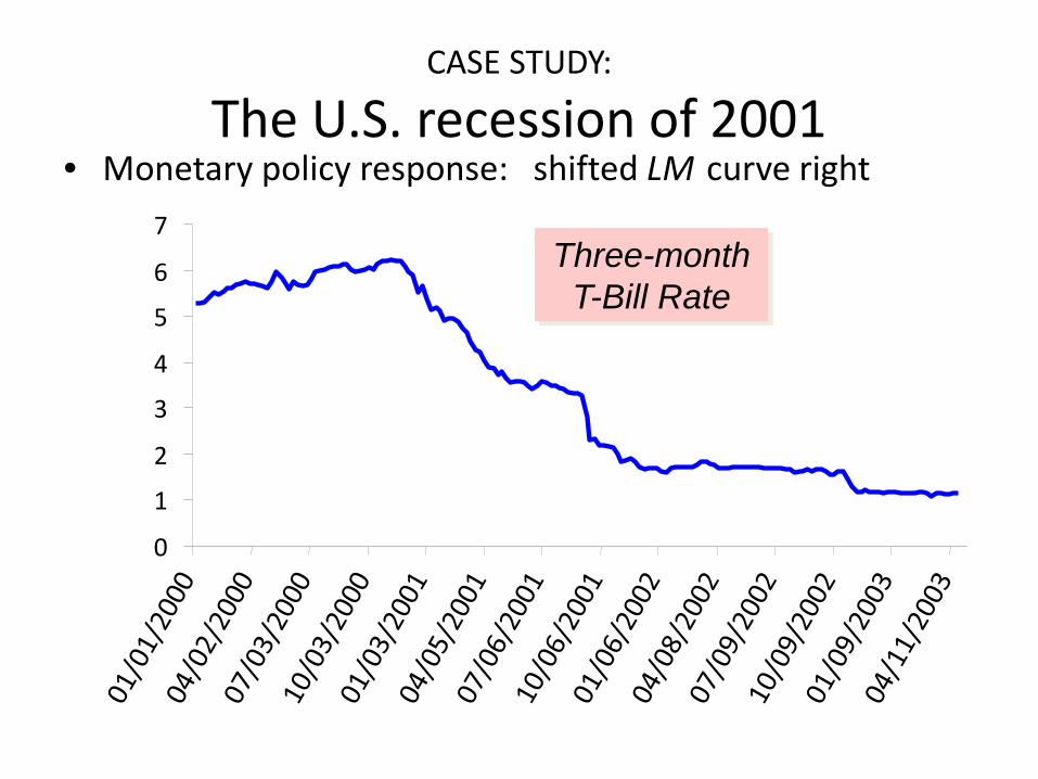
CASE STUDY:
The U.S. recession of 2001 • Monetary policy response: shifted LM curve right
Three-month T-Bill Rate
0
1
2
3
4
5
6
7
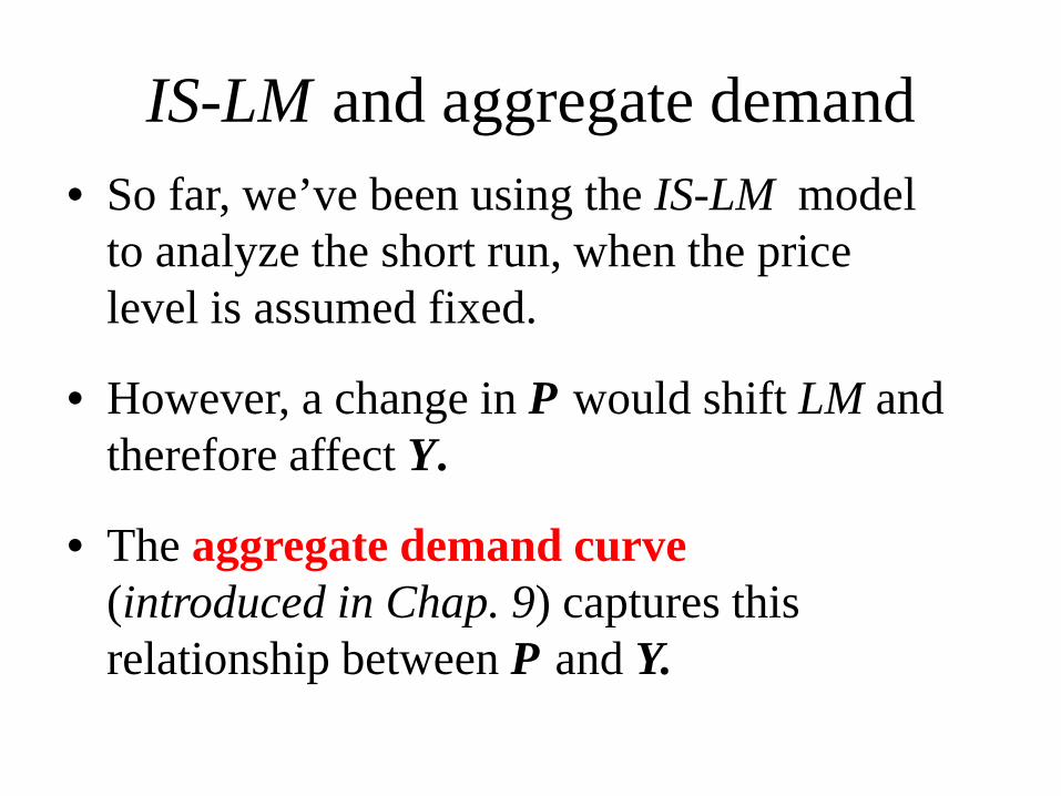
IS-LM and aggregate demand • So far, we’ve been using the IS-LM model
to analyze the short run, when the price level is assumed fixed.
• However, a change in P would shift LM and therefore affect Y.
• The aggregate demand curve (introduced in Chap. 9) captures this relationship between P and Y.

Y1 Y2
Deriving the AD curve
Y
r
Y
P
IS
LM(P1) LM(P2)
AD
P1
P2
Y2 Y1
r2
r1
Intuition for slope of AD curve:
↑P ⇒ ↓(M/P )
⇒ LM shifts left
⇒ ↑r
⇒ ↓I
⇒ ↓Y

Monetary policy and the AD curve
Y
P
IS
LM(M2/P1) LM(M1/P1)
AD1
P1
Y1
Y1
Y2
Y2
r1
r2
The Fed can increase aggregate demand:
↑M ⇒ LM shifts right
AD2
Y
r
⇒ ↓r
⇒ ↑I
⇒ ↑Y at each value of P
Y2
Y2
r2
Y1
Y1
r1
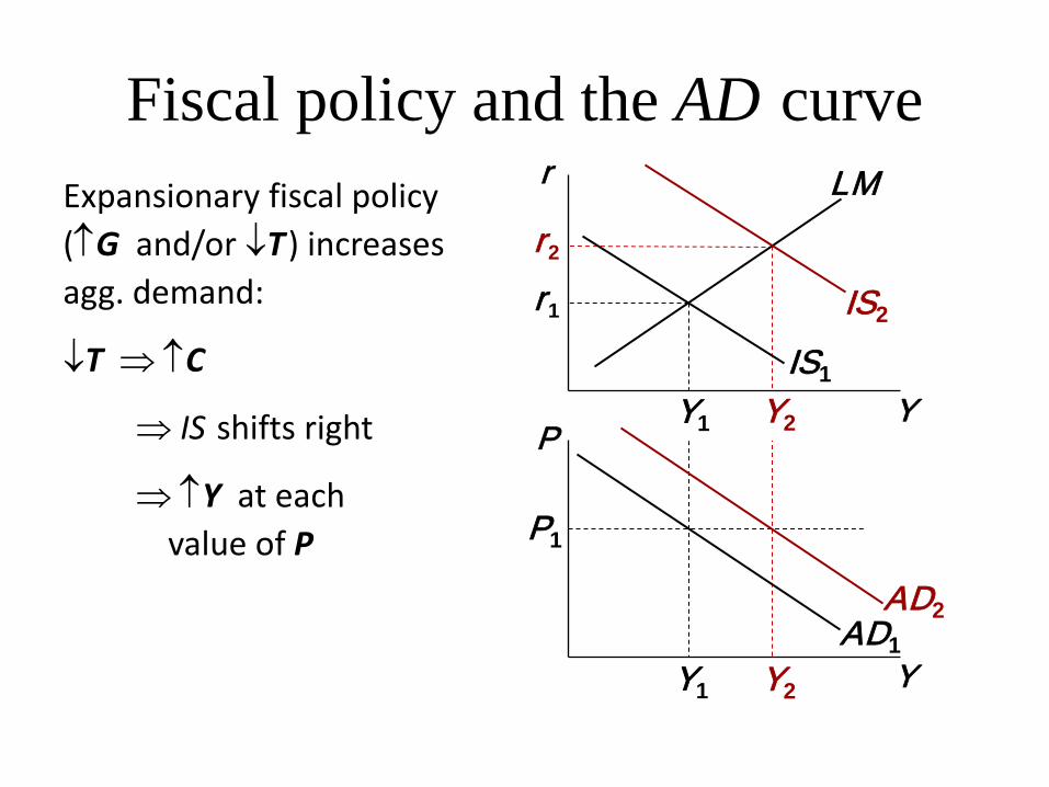
Fiscal policy and the AD curve
Y
r
Y
P
IS1
LM
AD1
P1
Expansionary fiscal policy (↑G and/or ↓T ) increases agg. demand:
↓T ⇒ ↑C
⇒ IS shifts right
⇒ ↑Y at each value of P
AD2
IS2

IS-LM and AD-AS in the short run & long run
Recall from Chapter 9: The force that moves the economy from the short run to the long run is the gradual adjustment of prices.
Y Y>
Y Y<
Y Y=
rise
fall
remain constant
In the short-run equilibrium, if
then over time, the price level will

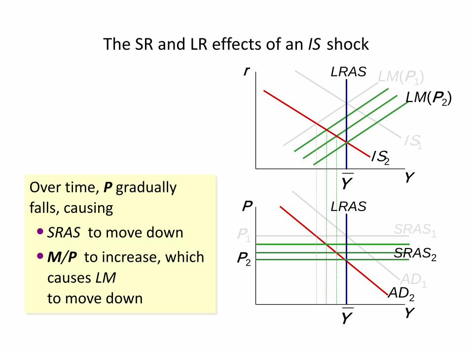
The SR and LR effects of an IS shock
A negative IS shock shifts IS and AD left, causing Y to fall.
Y
r
Y
P LRAS
Y
LRAS
Y
IS1
SRAS1 P1
LM(P1)
IS2
AD2
AD1

The SR and LR effects of an IS shock
Y
r
Y
P LRAS
Y
LRAS
Y
IS1
SRAS1 P1
LM(P1)
IS2
AD2
AD1
In the new short-run equilibrium, Y Y<

The SR and LR effects of an IS shock
Y
r
Y
P LRAS
Y
LRAS
Y
IS1
SRAS1 P1
LM(P1)
IS2
AD2
AD1
In the new short-run equilibrium, Y Y<
Over time, P gradually falls, causing •SRAS to move down •M/P to increase, which
causes LM to move down
AD2
The SR and LR effects of an IS shock
Y
r
Y
P LRAS
Y
LRAS
Y
IS1
SRAS1 P1
LM(P1)
IS2
AD1
SRAS2 P2
LM(P2)
Over time, P gradually falls, causing •SRAS to move down •M/P to increase, which
causes LM to move down
AD2
SRAS2 P2
LM(P2)
The SR and LR effects of an IS shock
Y
r
Y
P LRAS
Y
LRAS
Y
IS1
SRAS1 P1
LM(P1)
IS2
AD1
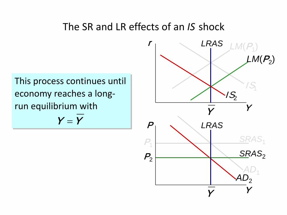
This process continues until economy reaches a long-run equilibrium with
Y Y=

NOW YOU TRY: Analyze SR & LR effects of ∆M
a. Draw the IS-LM and AD-AS diagrams as shown here.
b. Suppose Fed increases M. Show the short-run effects on your graphs.
c. Show what happens in the transition from the short run to the long run.
d. How do the new long-run equilibrium values of the endogenous variables compare to their initial values?
Y
r
Y
P LRAS
Y
LRAS
Y
IS
SRAS1 P1
LM(M1/P1)
AD1