Chapter 11Chapter 11

Simulating Wireless Control

Simulate Parameter – Analog Input BlockSimulate Parameter – Analog Input BlockSimulate Parameter – Analog Input BlockSimulate Parameter – Analog Input Block The current or digital outputs

of these transmitters and switches are normally accessed in a control system using the analog and discrete input blocks.

The normal processing of analog and discrete input blocks can be altered by enabling the Simulate parameter

Transfer of Simulation ParametersTransfer of Simulation ParametersTransfer of Simulation ParametersTransfer of Simulation Parameters Simulation modules may

be added without modifying existing modules if control systems include the capability for a module to read and write parameters contained in another module.

Using this capability, simulation modules may read the output value of analog and discrete output function blocks

.The results of the simulation modules may then be written back to the simulation input parameters.

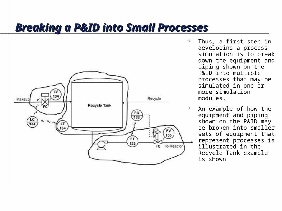
Breaking a P&ID into Small ProcessesBreaking a P&ID into Small ProcessesBreaking a P&ID into Small ProcessesBreaking a P&ID into Small Processes Thus, a first step in

developing a process simulation is to break down the equipment and piping shown on the P&ID into multiple processes that may be simulated in one or more simulation modules.

An example of how the equipment and piping shown on the P&ID may be broken into smaller sets of equipment that represent processes is illustrated in the Recycle Tank example is shown

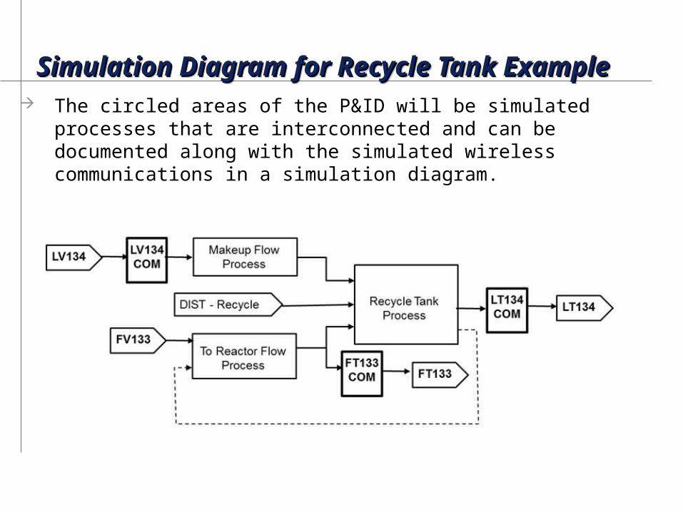
Simulation Diagram for Recycle Tank ExampleSimulation Diagram for Recycle Tank ExampleSimulation Diagram for Recycle Tank ExampleSimulation Diagram for Recycle Tank Example The circled areas of the P&ID will be simulated processes that are

interconnected and can be documented along with the simulated wireless communications in a simulation diagram.

Simulation Module Construction for Simulation Module Construction for Recycle Tank ExampleRecycle Tank ExampleSimulation Module Construction for Simulation Module Construction for Recycle Tank ExampleRecycle Tank Example

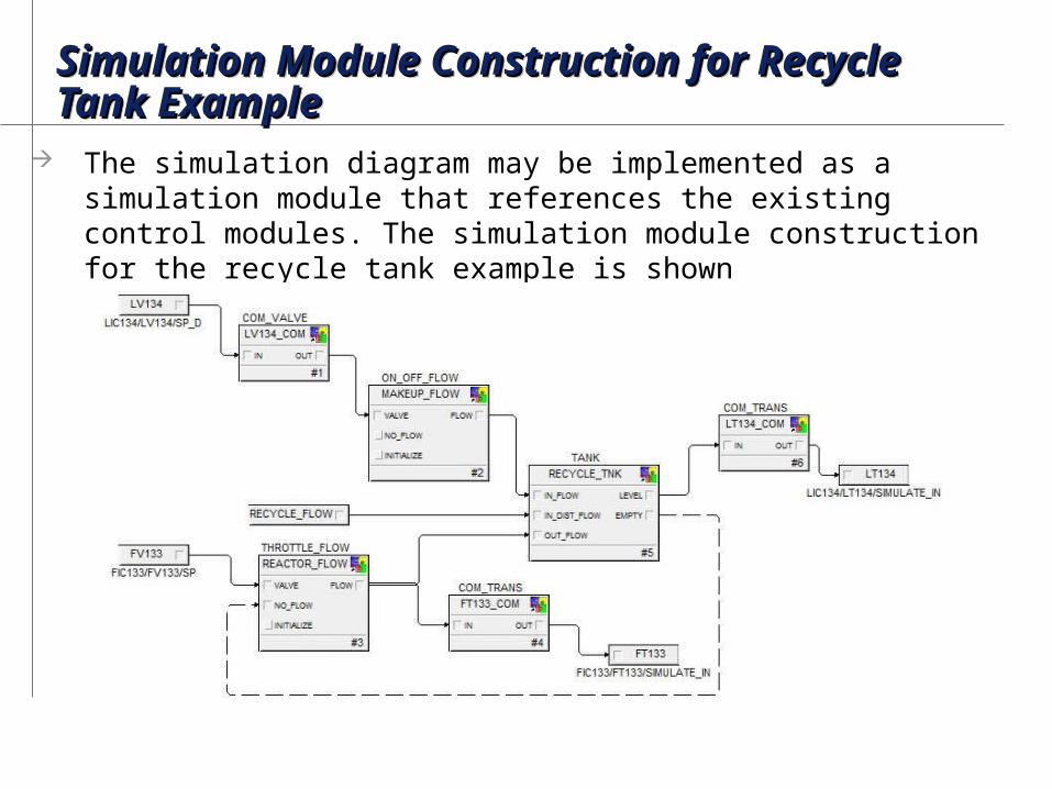
The simulation diagram may be implemented as a simulation module that references the existing control modules. The simulation module construction for the recycle tank example is shown

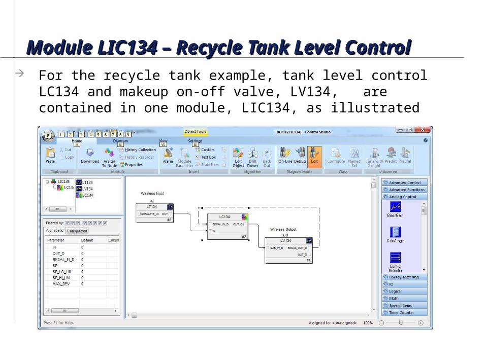
Module LIC134 – Recycle Tank Level ControlModule LIC134 – Recycle Tank Level ControlModule LIC134 – Recycle Tank Level ControlModule LIC134 – Recycle Tank Level Control For the recycle tank example, tank level control LC134 and makeup

on-off valve, LV134, are contained in one module, LIC134, as illustrated

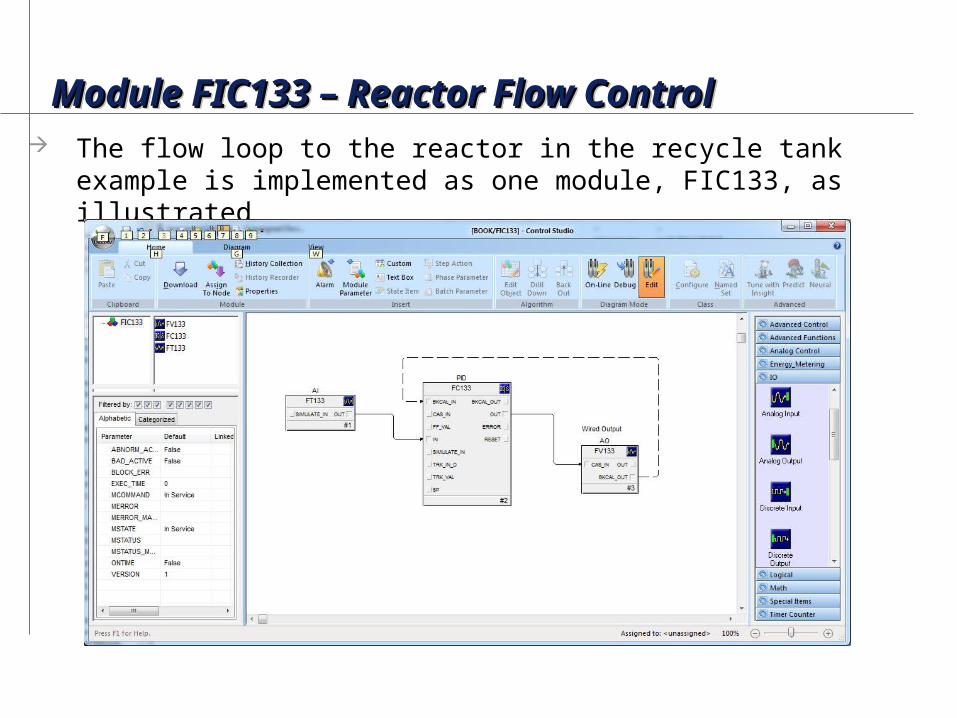
Module FIC133 – Reactor Flow ControlModule FIC133 – Reactor Flow ControlModule FIC133 – Reactor Flow ControlModule FIC133 – Reactor Flow Control The flow loop to the reactor in the recycle tank example is

implemented as one module, FIC133, as illustrated

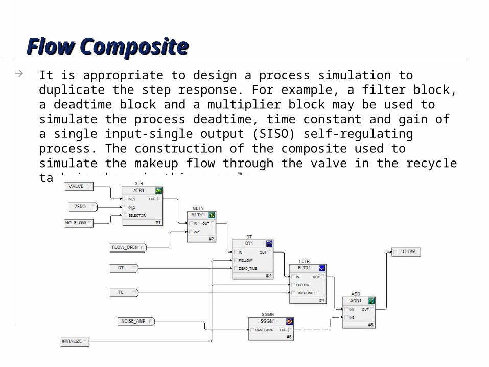
Flow CompositeFlow CompositeFlow CompositeFlow Composite It is appropriate to design a process simulation to duplicate the step response.

For example, a filter block, a deadtime block and a multiplier block may be used to simulate the process deadtime, time constant and gain of a single input-single output (SISO) self-regulating process. The construction of the composite used to simulate the makeup flow through the valve in the recycle tank is shown in this example

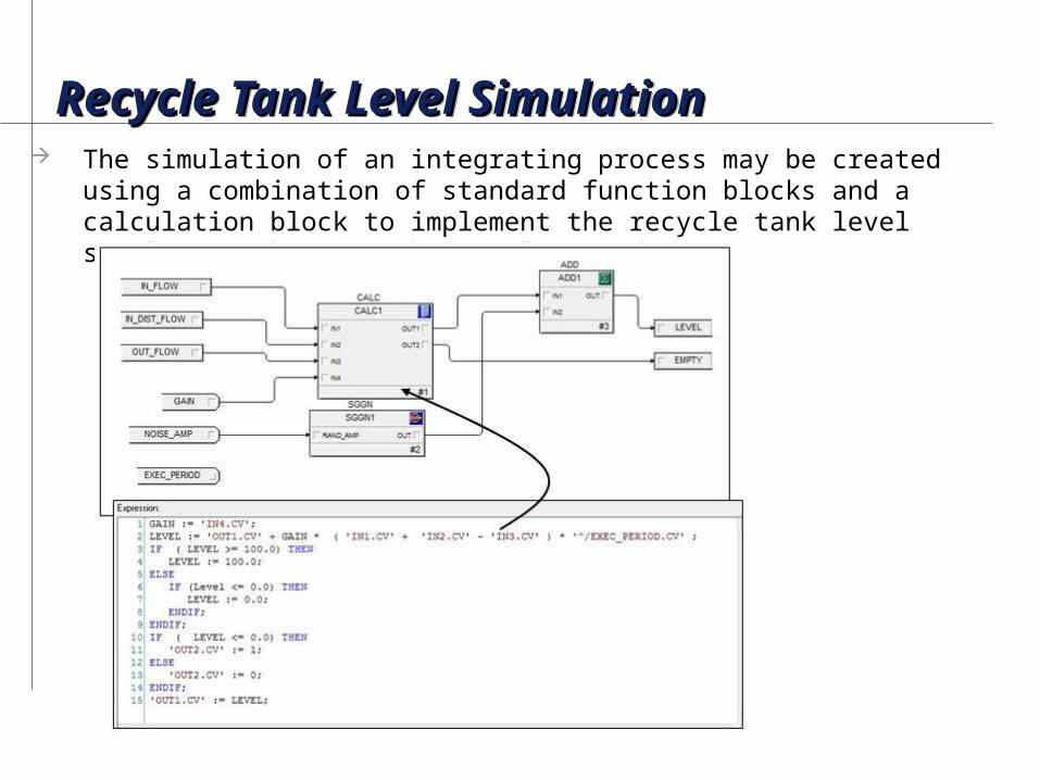
Recycle Tank Level SimulationRecycle Tank Level SimulationRecycle Tank Level SimulationRecycle Tank Level Simulation The simulation of an integrating process may be created using a combination

of standard function blocks and a calculation block to implement the recycle tank level simulation shown in the Simulation diagram

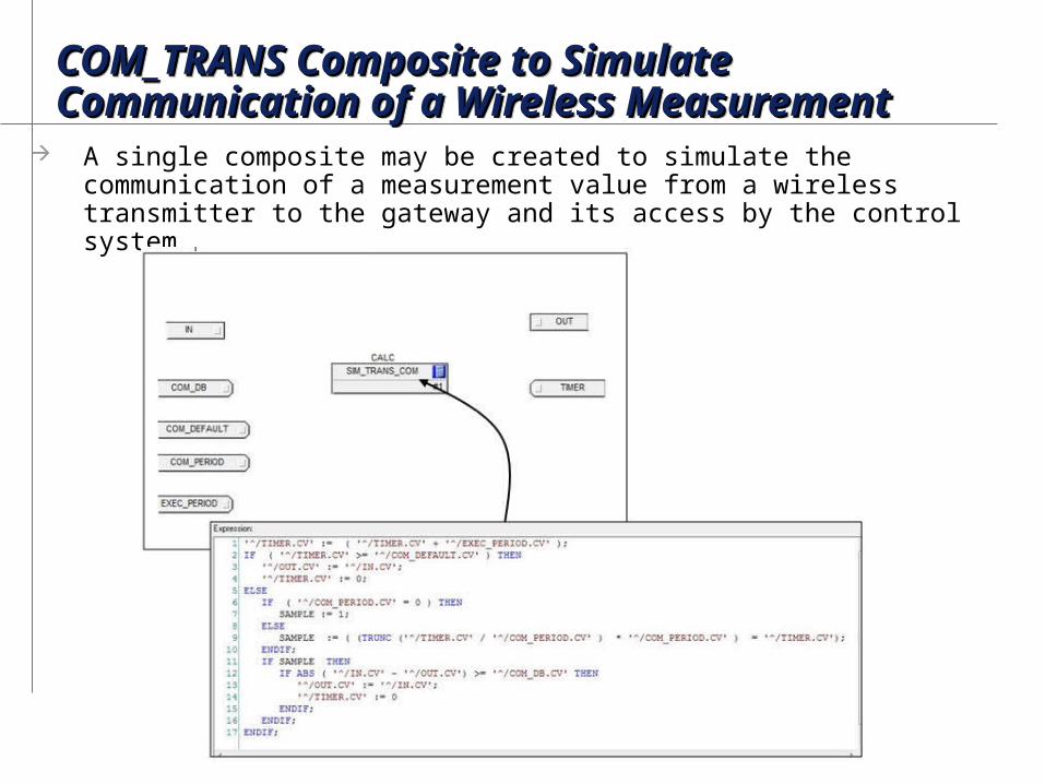
COM_TRANS Composite to Simulate COM_TRANS Composite to Simulate Communication of a Wireless MeasurementCommunication of a Wireless MeasurementCOM_TRANS Composite to Simulate COM_TRANS Composite to Simulate Communication of a Wireless MeasurementCommunication of a Wireless Measurement

A single composite may be created to simulate the communication of a measurement value from a wireless transmitter to the gateway and its access by the control system.

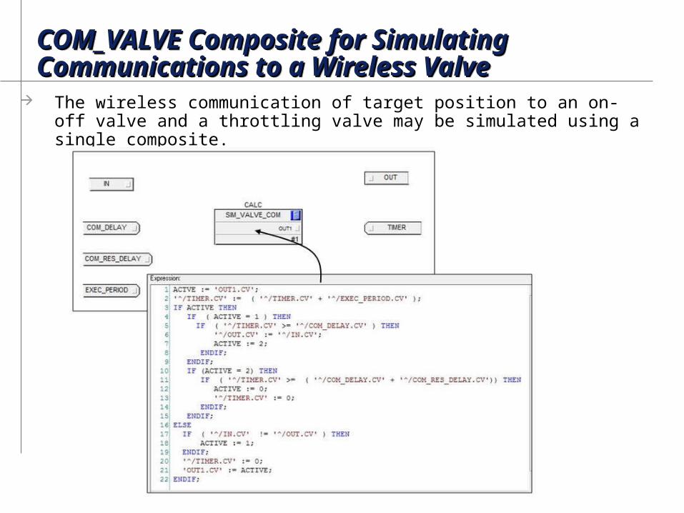
COM_VALVE Composite for Simulating COM_VALVE Composite for Simulating Communications to a Wireless Valve Communications to a Wireless Valve COM_VALVE Composite for Simulating COM_VALVE Composite for Simulating Communications to a Wireless Valve Communications to a Wireless Valve

The wireless communication of target position to an on-off valve and a throttling valve may be simulated using a single composite.

Example Simulation InterfaceExample Simulation InterfaceExample Simulation InterfaceExample Simulation Interface

Some control systems provide simulation environments that allow process simulation modules and control modules to provide faster than real-time response.

Such tools may also allow the input block’s Simulate parameter to be enabled or disabled in all modules or in selected modules with one click of a button.

This is an example of the interface provided for such a simulation environment

Exercise: Simulating Wireless ControlExercise: Simulating Wireless ControlExercise: Simulating Wireless ControlExercise: Simulating Wireless Control

This workshop exercise is designed to further explore the implementation of the process and wireless communication simulation for a recycle.

Step 1: Open the module that simulates the recycle tank process and wireless communication and compare this to the P&ID shown below.

Step 2: Examine the off-line and on-line view of the composites that were created to simulate the wireless communication from a transmitter to the control system. Examine the composites created to and to a simulation the communication of the target valve position to the wireless valve.

Step 3: Using a trend of the tank level, the on-off valve position and the flow to the reactor, examine how the on-off recycle valve is manipulated by LC134 to keep the tank level from going below a level setpoint..

Step 4: Adjust the setpoint of FIC133 to change the flow rate to the reactor. Using a trend of the flow measurement and valve position, examine how PIDPlus regulates the valve to achieve the new flow setpoint. How does the flow change impact the level control?

Step 5: Reduce the recycle flow input and observe the impact on how frequently the recycle flow is activated.

Process: Simulating Wireless ControlProcess: Simulating Wireless ControlProcess: Simulating Wireless ControlProcess: Simulating Wireless ControlThis workshop exercise is designed to show how a simulation of a process and associated wireless field devices may be constructed and used in control system checkout. A recycle tank is used as a process example.

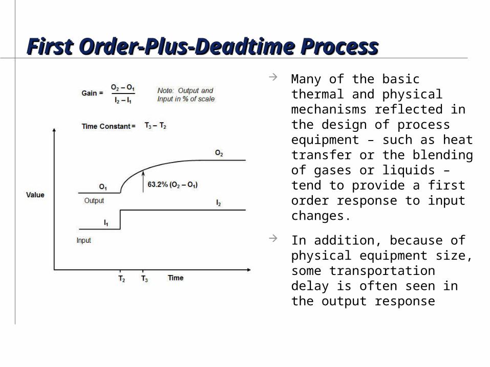
First Order-Plus-Deadtime Process First Order-Plus-Deadtime Process First Order-Plus-Deadtime Process First Order-Plus-Deadtime Process Many of the basic thermal and

physical mechanisms reflected in the design of process equipment – such as heat transfer or the blending of gases or liquids – tend to provide a first order response to input changes.

In addition, because of physical equipment size, some transportation delay is often seen in the output response

Heater Example – First Order-Plus-Heater Example – First Order-Plus-Deadtime ProcessDeadtime ProcessHeater Example – First Order-Plus-Heater Example – First Order-Plus-Deadtime ProcessDeadtime Process

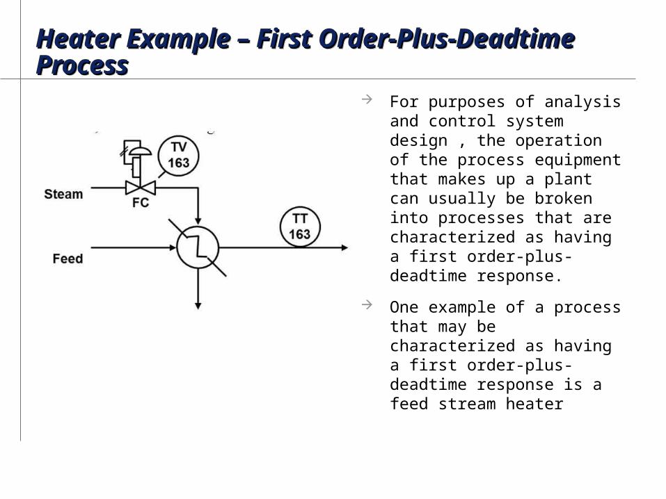
For purposes of analysis and control system design , the operation of the process equipment that makes up a plant can usually be broken into processes that are characterized as having a first order-plus-deadtime response.

One example of a process that may be characterized as having a first order-plus-deadtime response is a feed stream heater

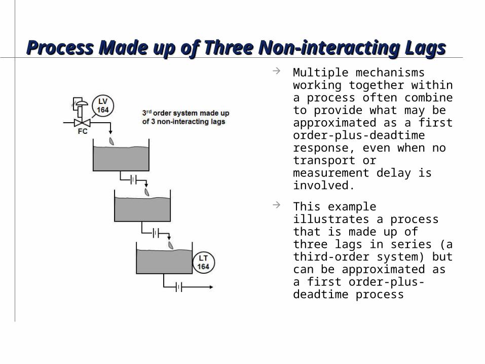
Process Made up of Three Non-interacting Lags Process Made up of Three Non-interacting Lags Process Made up of Three Non-interacting Lags Process Made up of Three Non-interacting Lags Multiple mechanisms

working together within a process often combine to provide what may be approximated as a first order-plus-deadtime response, even when no transport or measurement delay is involved.

This example illustrates a process that is made up of three lags in series (a third-order system) but can be approximated as a first order-plus-deadtime process

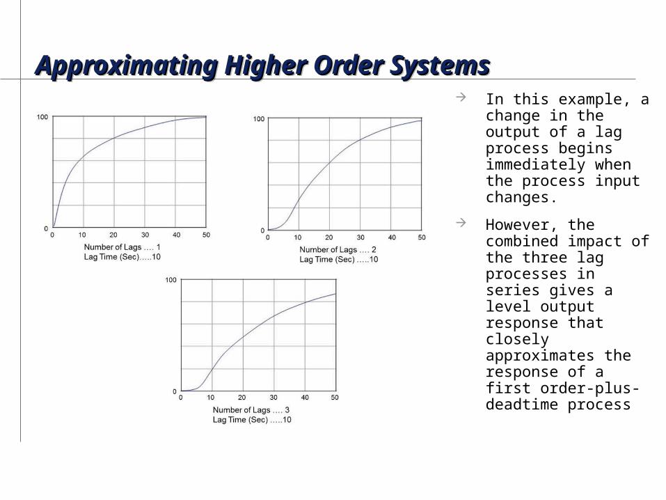
Approximating Higher Order SystemsApproximating Higher Order SystemsApproximating Higher Order SystemsApproximating Higher Order Systems In this example, a

change in the output of a lag process begins immediately when the process input changes.

However, the combined impact of the three lag processes in series gives a level output response that closely approximates the response of a first order-plus-deadtime process

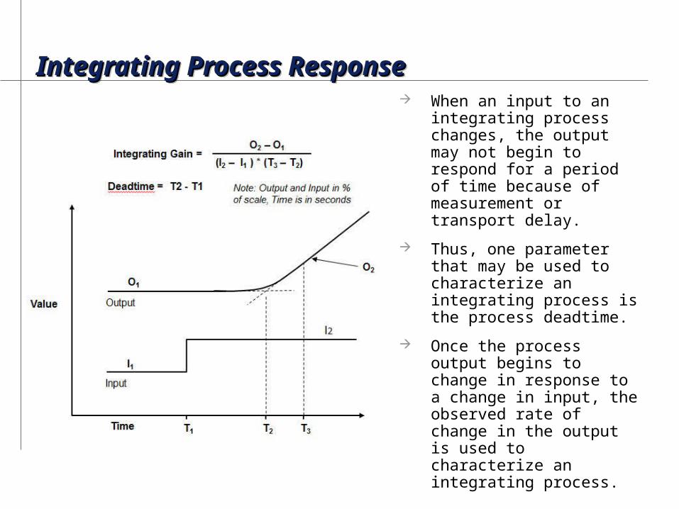
Integrating Process Response Integrating Process Response Integrating Process Response Integrating Process Response When an input to an

integrating process changes, the output may not begin to respond for a period of time because of measurement or transport delay.

Thus, one parameter that may be used to characterize an integrating process is the process deadtime.

Once the process output begins to change in response to a change in input, the observed rate of change in the output is used to characterize an integrating process.

Example – Integrating ProcessExample – Integrating ProcessExample – Integrating ProcessExample – Integrating Process Integrating processes are also

described as non-self-regulating processes.

An example of an integrating process is a tank in which the flow into the tank is the manipulated input, the tank level is the controlled output, and the discharge from the tank is a gear pump.

In this process, the outlet flow rate is determined by the speed of the gear pump and thus is not affected by the tank level.

Simulation of a Multivariate Process Simulation of a Multivariate Process Simulation of a Multivariate Process Simulation of a Multivariate Process

When the response of a process that has multiple inputs and/or outputs is addressed, the assumption made in simulating the process by step responses is that the process is linear and possesses the two properties of superposition and homogeneity. These properties are the basis on which the process output of a multivariable process may be represented by the sum of the step responses for a change in the process inputs, as illustrated. Every process output is the sum of input actions.