Chapter 10Wave-to-Wire Modelling of WECs

Marco Alves

10.1 Introduction

Numerical modelling of wave energy converters (WECs) of the wave activatedbody type (WAB, see Chap. 2) is based on Newton’s second law, which states thatthe inertial force is balanced by all forces acting on the WEC’s captor. These forcesare usually split into hydrodynamic and external loads.

In general, the hydrodynamic source comprises the (more details in Chap. 6):

• Hydrostatic force caused by the variation of the captor submergence due to itsoscillatory motion under a hydrostatic pressure distribution,

• Excitation loads due to the action of the incident waves on a motionless captor,• Radiation force corresponding to the force experienced by the captor due to the

change in the pressure field as result of the fluid displaced by its own oscillatorymovement, in the absence of an incident wave field.

Depending on the type of WEC, the external source may include the loadsinduced by the

• Power-take-off (PTO) equipment, which converts mechanical energy (captormotions) into electricity (more details in Chap. 8),

• Mooring system, responsible for the WEC station-keeping (more details inChap. 7),

• End-stop mechanism, used to decelerate the captor at the end of its stroke inorder to dissipate the kinetic energy gently, and therefore avoid mechanicaldamage to the device.

M. Alves (&)Rua Dom Jerónimo Osório 11, 1400-119 Lisbon, Portugale-mail: marco@wavec.org

© The Author(s) 2017A. Pecher and J.P. Kofoed (eds.), Handbook of Ocean Wave Energy,Ocean Engineering & Oceanography 7, DOI 10.1007/978-3-319-39889-1_10

261

The hydrodynamic modelling of the interaction between ocean waves (seeChap. 3) and WECs is often split into three different phases according to the seaconditions:

(i) During small to moderate sea states linear wave approximations are valid,corresponding to the current state-of-the-art methods of hydrodynamicmodelling.

(ii) Under moderate to extreme waves, in general, some sort of non-linearhydrodynamic modelling is required in order to more accurately model thewave/device interaction.

(iii) Ultimately, under stormy conditions, a fully non-linear approach is neces-sary to model the hydrodynamic interaction of the waves and the device.

With respect to the modelling of the external loads it is commonly accepted thatthe production of energy should be restricted to non-stormy conditions (WECoperating mode), comprising both small to moderate and moderate to extremewaves, which correspond to low and intermediate energetic sea states. Understormy conditions, usually it is not necessary to model the dynamics of the PTOequipment as the WEC is interacting with extreme waves and so it must assume thesurvivability mode with no energy production. In the operating mode of the devicethe loads induced by the PTO equipment, the mooring system and the end-stopmechanism may be linearized under certain assumptions; however, typically theyexhibit strongly nonlinear behaviour, which requires a time domain approach inorder to be described properly.

Although the scope of this chapter is confined to wave-to-wire modelling it isimportant to emphasize that there are other modelling methods and that the mostadequate one depends on several factors such as the required accuracy (which istypically inversely proportional to the computational time), the sea state (stormy ornon-stormy conditions), the device regime (operational or survival mode) and itswork principle (some concepts exhibit more non-linear behaviours). In view of that,the modelling tools are typically split into 3 different types:

1 Frequency models: The hydrodynamic interaction between WECs and oceanwaves is a complex high-order non-linear process, which, under some particularconditions, might be simplified. This is the case for waves and device oscillatorymotions of small-amplitude. In this case the hydrodynamic problem is wellcharacterised by a linear approach. Therefore, in such a framework (which isnormally fairly acceptable throughout the device’s operational regime), and withlinear forces imposed by both the PTO and the anchoring system, the first step tomodel the WEC dynamics is traditionally carried out in the frequency domain(where the excitation is of a simple harmonic form). Consequently, all thephysical quantities vary sinusoidally with time, according to the frequency ofthe incident wave. Under these circumstances, the equations of motion become alinear system that may be solved in a straightforward manner.Although frequency models have limited applicability, being restricted to linearproblems where the superposition principle is valid, the frequency domain

262 M. Alves

approach is extremely useful as it allows for a relatively simple and fastassessment of the WEC performance, under the aformentioned conditions.Hence, this approach is generally used to optimise the geometry of WECs inorder to maximize the energy capture [1–3].

2 Wave-to-wire models (time domain tools): Besides the interest of the frequencydomain approach, in many practical cases the WEC dynamics has some partsthat are strongly non-linear, and so the superposition principle is no longerapplicable. These nonlinearities arise mostly from the dynamics of the mooringsystem, the PTO equipment and control strategy and, when present, the end-stopmechanism. Furthermore, under moderate to extreme waves, nonlinear effects inthe wave/device hydrodynamic interaction are more relevant. This requiressome sort of non-linear modelling that typically consists of treating the buoy-ancy and the excitation loads as non-linear terms. In addition, second-order slowdrift forces may be also included in a time domain description of the WECdynamics (this force must be undertaken by the station-keeping system). Toproperly account for these nonlinearities the WEC modelling has to be per-formed in time domain. Moreover, the motion of the free surface in a sea staterarely reaches steady-state conditions, and so must also be represented in thetime domain.The time domain approach is a reasonably detailed and accurate description of theWEC dynamics. Since this approach allows modelling of the entire chain of energyconversion from the wave/device hydrodynamic interaction to feeding into theelectrical grid, time domain models are commonly named wave-to-wire codes. Themost relevant outcomes of a wave-to-wire code includes, among others, estimatesof the instantaneous power produced under irregular sea states,motions/velocities/accelerations of the WEC captor and loads on the WEC. Besides,wave-to-wire models are extremely useful tools to optimize the WEC controlstrategy in order to maximize the power captured. The Structural Design of WaveEnergy Devices (SDWED) project, led by Aalborg University, has generated acomprehensive set of free software tools including advanced hydrodynamic models,spectral fatigue models and wave to wire models [4].

3 Computational fluid dynamics—CFD: Due to the large computational timethe use of CFD codes is typically restricted to study the wave/device interac-tion under extreme waves, which is a strongly non-linear phenomena. Normally,the main objective in this case is to model the WEC dynamics in its survivalmode with no energy production (in order to evaluate the suitability of thesurvival strategy). This type of wave-body interaction is usually computedsolving the Reynolds Averaged Navier-Stokes Equations (RANSE1) with some

1The decomposing of the Navier-Stokes equations into the Reynolds-averaged Navier–Stokesequations (RANSE) makes it possible to model complex flows, such as the flow around a wavepower device. RANSE are based on the assumption that the time-dependent turbulent velocityfluctuations may be separated from the mean flow velocity. This assumption introduces a set ofunknowns, named the Reynolds stresses (functions of the velocity fluctuations), which require aturbulence model to produce a closed system of solvable equations.

10 Wave-to-Wire Modelling of WECs 263

sort of numerical technique to model the free surface of the water. Amongseveral different methods to model the free surface one of the most commonlyused is the Volume of Fluid (VoF) [5]. At present there are some CFD codescapable of modelling this sort of wave-body interaction and flows with complexfree-surface phenomena such as wave breaking and overtopping (see Sect. 10.3:Benchmark Analysis).

10.2 Wave-to-Wire Models

At present there are many designs being pursued by developers to harness wavepower, which may be categorized according to the location and depth in which theyare designed to operate, i.e. shoreline, near shore or offshore, or by the type ofpower capture mechanism. However, there is no common device categoriza-tion that has been widely accepted within the international research and technologydevelopment community, but the most popular distinguishing criteria is based ontheir operational principle. According to this criterion WECs are usually dividedinto six distinct classes: attenuators; point absorbers; oscillating-wave surge con-verters; oscillating water columns (OWC); overtopping devices; and submergedpressure-differential devices [6]. These categories may be regrouped into threefundamentally different classes, namely OWC, WECs with wave-induced relativemotions and overtopping devices. For WECs within the two first fundamentalclasses the generic approach to develop wave-to-wire models presented herein isvalid, however, for overtopping concepts the performance analysis requires the usedifferent type of numerical tools based on empirical expressions (such as e.g.WOPSim: Wave Overtopping Power Simulation [7]) or CFD codes.

In the field of wave energy, the term wave-to-wire refers to numerical tools thatare able to model the entire chain of energy conversion from the hydrodynamicinteraction between the ocean waves and the WEC to the electricity feed into thegrid. In terms of complexity, and consequently time expenditure, these types ofnumerical tools are in-between frequency domain codes, which are much faster butless accurate (because all the forces are linearized), and CFD codes, which arecurrently the most precise numerical tools available, but also extremely timedemanding, which makes their use unviable to solve the majority of problems inthis field.

This section presents a discussion on the assumptions, considerations andtechniques commonly used in developing wave-to-wire models, highlighting thelimitations and the range of validity of this type of modelling tool. A generaldiscussion is presented aiming to embrace the majority of existing WECs, never-theless when appropriate, an annotation regarding the fundamental differences inthe working principle of some particular WECs and the subsequent adjustments inthe wave-to-wire model will be made.

264 M. Alves

10.2.1 Equation of Motion

In essence, the algorithm to build a wave-to-wire model relies on Newton’s secondlaw of motion, which states that the inertial force is balanced by all of the forcesacting on the WEC’s captor. This statement is expressed by the equation

M€nðtÞ ¼ FeðtÞþFrðtÞþFhsðtÞþFf ðtÞþFptoðtÞþFmðtÞ; ð10:1Þ

where M represents the mass matrix and €n the acceleration vector of the WEC. Theterms on the right hand side of Eq. 10.1 correspond to:

• The excitation loads—Fe

• The hydrostatic force—Fhs

• The friction force—Ff

• The radiation force—Fr

• The PTO loads—Fpto

• The mooring loads—Fm

In the following section a discussion on the different sources of loads on theWEC captor is presented and their impact on the overall dynamics of the WEC isgiven in order to substantiate the assumptions and simplifications commonly con-sidered in the development of wave-to-wire codes.

10.2.2 Excitation Force

The excitation force results from the pressure exerted on the body’s wetted surfacedue to the action of the incoming waves. The most popular approach to computethis force is based on linear wave theory, in which the body is assumed to bestationary and the area of the wetted surface constant and equal to the value inundisturbed conditions. Obviously this assumption is only valid for small waveamplitudes, which is a fundamental assumption of linear theory. Therefore, underlinear assumptions the excitation load on the WEC captor is given by

FexcðtÞ ¼Z1

�1fexc t � sð ÞgðsÞds; ð10:2Þ

where η is the free surface elevation due to the incident wave (undisturbed by theWEC) at the reference point where the WEC is located and fexc is the so calledexcitation impulse response function derived from the frequency coefficientscommonly obtained with a 3D radiation/diffraction code (see Sect. 10.3).Equation 10.2 shows that it is necessary to model the random sea state behaviour inorder to estimate the excitation force. The most common approach consists of usingAiry wave theory, a linear theory for the propagation of waves on the surface of a

10 Wave-to-Wire Modelling of WECs 265

potential flow and above a horizontal bottom. The free surface elevation, η, may bethen reproduced for a wave record with duration T as the sum of a large (theo-retically infinite) number, N, of harmonic wave components (a Fourier series), theso called wave superposition method, as

gðtÞ ¼XNi¼1

ai cosð2pfi tþ aiÞ; ð10:3Þ

where, t is the time, ai and ai the amplitudes and phases of each frequency,respectively, and fi ¼ i=T . The phases are randomly distributed between 0 and 2p,so the phase spectrum may be disregarded. Hence, to characterize the free surfaceelevation only the amplitudes of the sinusoidal components need to be identified,which are given by

ai ¼ffiffiffiffiffiffiffiffiffiffiffiffiffiffiffiffiffiffi2Sf ðfiÞDf

q; ð10:4Þ

where Sf is the variance density spectrum or simply energy spectrum (see Fig. 10.1)and Df the frequency interval. As only the frequencies fi are presented in the energyspectrum, while in reality all frequencies are present at sea, it is convenient to let thefrequency interval Df ! 0: The spectrum of energy is usually plotted as energydensity, (unit of energy/unit frequency interval, Hz) given by the amount of energyin a particular frequency interval.

For more realistic descriptions of the wave surface elevation the wave’s direc-tionality must be considered. In this case the direction resolved spectrum Sðb; f Þ,dependent on the frequency, f, and wave direction, b, is written as

Sf ðf ; bÞ ¼ Dðf ; bÞSf ðf Þ; ð10:5Þ

0.05 0.10 0.15 0.20 0.25

1

2

3

4

ycneuqerF )zH(f

vari

ance

den

sity

Sf(f)

(m2 a)

Fig. 10.1 Typical variancedensity spectrum

266 M. Alves

where the directional distribution Dðb; f Þ is normalized, satisfying the condition

Zp

�p

Dðb; f Þdb ¼ 1: ð10:6Þ

The spectrum is defined with several parameters in which the most importantones are the significant wave height, denoted by Hs or H1=3 (which corresponds tothe average of the highest third of the waves), and the peak period, Tp corre-sponding to the period with the highest peak of the energy density spectrum (thespectrum may have more than one peak).

10.2.3 Hydrostatic Force

When a body is partially or completely immersed in a liquid it will experience anupward force (buoyancy) equal to the weight of the liquid displaced, which isknown as Archimedes’ principle. The hydrostatic force results from the differencebetween this upward force and the weight of the body. Accordingly, the variation ofthe captor submergence due to its oscillatory motion under a hydrostatic pressuredistribution causes a change in the buoyancy (equal to the change of weight ofdisplaced fluid) and hence a variation in the hydrostatic force.

A fundamental assumption of linear theory is that the resulting body motions areof small amplitude, which normally conforms with the behaviour of WECs duringthe operational regime. In fact, the motion of WECs tends to be of small amplitudebecause otherwise the dissipative viscous effects would be dominant in the devicedynamics, which would ultimately limit the motion and reduce the device effi-ciency. Therefore, the hydrostatic force, Fhs, is commonly implemented inwave-to-wire models merely as a function proportional to the body displacement,where the proportionality coefficient is known as the hydrostatic coefficient, i.e.,

FhsðtÞ ¼ GzðtÞ; ð10:7Þ

where G is the hydrostatic coefficient and z the motion in the direction of the degreeof freedom (DoF) being considered. In the case of several DoFs being analysedG and z represent the hydrostatic matrix and the displacement vector, respectively.

For example, in the case of a heaving body undergoing small-amplitude oscil-lations the variation of the buoyancy force may be simply given by

FhsðtÞ ¼ qgAzðtÞ; ð10:8Þ

where q denotes the water density, g the gravitational acceleration, A the cross sectionalarea of the body in undisturbed conditions and z its vertical displacement. The variationof the volume of water displaced by the oscillating body is equal to the variation of its

10 Wave-to-Wire Modelling of WECs 267

submerged volume, given by Az. We should note that typically the assumption ofconstant cross sectional area along the vertical axis is only valid for motions ofsmall-amplitude. Depending on the body geometry, typically this simplification (basedon the linear wave theory) is not valid for large-amplitude motions where in general thevariation of the cross-sectional area is more noticeable, and so a non-linear approach isrequired to accurately assess the hydrostatic force.

10.2.4 Mooring Loads

Wave drift forces,2 along with currents and wind, have a tendency to push the WECaway from the deployment position. To prevent this drifting, the WEC should bemaintained in position by a station-keeping system, also commonly calleda “mooring system”. The station-keeping system is usually designed to withstandsurvival conditions, e.g. 100 year storm conditions. The moorings designed forfloating WECs are required to limit their excursions and, depending on the concept,aligning its position according to the angle of incidence of the incoming waves.Moreover, unlike typical offshore structures, the mooring design has an additionalrequirement of ensuring efficient energy conversion, since it may change theresponse of the WEC and so change its ability to capture wave energy.

Depending on the working principle of the device and ultimately the manner inwhich the mooring system provides the restoring force, mooring systems might bepassive, active or reactive. Passive mooring systems are designed for the uniquepurpose of station-keeping. Conversely, active mooring systems have a strongerimpact on the dynamic response of WECs since the system stiffness may be used toalter the resonant properties of WECs. Ultimately, reactive mooring systems areapplied when the PTO exploits the relative movements between the body and thefixed ground, such that the mooring system provides the reaction force. In thismooring configuration the inboard end of the mooring line/s is connected to thePTO equipment which controls the tensions or loosens of the mooring line/s inorder to adjust the WEC position according to the established control strategy.A review of design options for mooring systems for wave energy converters ispresented in Refs. [8, 9].

Mooring systems are traditionally composed of several mooring lines (slack ortaut), with one extremity attached to the device, at a point called the fairlead, andthe other extremity attached to a point that must be able to handle the loads appliedby the device through the line. This point can be fixed to an anchor on the seabed,or moving, e.g. the fairlead on another floating offshore structure. Mooring lines are

2Drift forces are second-order low frequency wave force components. Under the influence of theseforces, a floating body will carry out a steady slow drift motion in the general direction of wavepropagation if it is not restrained. See further in Chap. 7.

268 M. Alves

usually composed of various sections of different materials (chain, wired-ropes,polyester, etc.). Some additional elements, such as floats or clump weights can beattached to the line to give it a special shape.

Depending on the objectives of the simulation, the mooring system can bemodelled with different levels of accuracy, and thus different computational efforts.Hence, it is important to understand the level of detail and accuracy required inorder to select the most appropriate modelling approach. Essentially mooringmodels may be split into two main categories: quasi-static and dynamic models.

Quasi-static models depend only on the position of the fairlead and the anchor atspecific time-step. Therefore, they do not solve differential equations for the motionof the lines, which considerably reduces the required computational effort.Quasi-static models may be split into two types:

• Linearized mooring model. The most common quasi-static model is theso-called “linearized mooring model” which consists of modelling the mooringloads in the different directions of motion by a simple spring effect. The com-putation of the restoring effect is straightforward, but it is only effective whenthe device has small motions, around its undisturbed position. Whenever thisapproach is built-in in the wave-to-wire model it is necessary to input themooring spring stiffness matrix (which is multiplied by the displacement vectorat each time-step to define the tension at the fairlead connection).

• Quasi-static catenary model. The quasi-static catenary modelling approachconsists of computing the tension applied by a catenary mooring line on a deviceusing only the position of the fairlead and the anchor. This mooring modellingapproach requires the inclusion of the nonlinear quasi-static catenary lineequations in the wave-to-wire model, which are solved at each time-step inorder to determine the value of the tension at the fairleads. This modellingapproach is very simple and requires little computational effort, but it is onlyvalid for relatively small motions about the mean position.

Quasi-static models are usually reliable to estimate the horizontal restoring effecton a device that experiences small motion amplitudes, but they are not reliable toestimate the effective tension in the line, especially in extreme weather conditions.In this case, dynamic models are necessary to compute the loads in the lines, andthus the restoring effect of the station-keeping system. This feature is available insome commercial modelling software such as OrcaFlex3 [10] or ANSYS AQWA[11]. Although wave-to-wire tools may be coupled to dynamic mooring models this

3Dynamic models represent the mooring lines by a finite-element description. The equation ofmotion is solved at each node in order to compute the tension in the line. Consequently, theelasticity and stiffness of the line, the hydrodynamic added-mass and drag effects, and the seabedinteractions, among others, can be modelled accurately. The numerical methods implemented insuch codes allow making numerical predictions under extreme loads and fatigue analysis ofmooring lines possible, however, the computational effort required is in general considerable. Themost widespread commercial code available in the market is Orcaflex a user-friendly numericaltool that allows the user to study the most common problems in offshore industry.

10 Wave-to-Wire Modelling of WECs 269

is not a common approach. Wave-to-wire tools are designed to model the opera-tional regime of WECs (i.e. during power production) where a linear (or partiallynon-linear) wave/device hydrodynamic interaction is fairly valid. In general, thenonlinear behaviour of WECs under extreme wave conditions is not properlyrepresented in wave-to-wire tools. Therefore, combining wave-to-wire and dynamicmooring models does not allow the full capabilities of the dynamic model to beexploited. Moreover, usually most WECs need to enter a survival mode (with noenergy production) in extreme wave conditions in order to avoid structural damagewhich, to some extent, decreases the usefulness of wave-to-wire models since theirmain feature is to assess the energy conversion efficiency.

10.2.5 Radiation Force

In addition to the usual instantaneous forces proportional to the acceleration,velocity and displacement of the body, the most commonly-used formulations oftime-domain models of floating structures incorporate convolution integral terms,known as ‘memory’ functions. These take account of effects which persist in thefree surface after motion has occurred. This ‘memory’ effect means that the loads onthe wet body surface in a particular time instant are partially caused by the changein the pressure field induced by previous motions of the body itself. Assuming thatthe system is causal, this is, h tð Þ ¼ 0 for t\0, and time invariant4 these convolutionintegrals take the form

FrðtÞ ¼Zs

0

h t � sð Þ_zðsÞds; ð10:9Þ

where h t � sð Þ represents the impulse-response functions (IRFs) or kernels of theconvolutions and _z sð Þ the body velocity towards any DoF. In the case of 6 rigidDoFs, h t � sð Þ is a 6 � 6 symmetric matrix where the off-diagonal entries representthe cross-coupling radiation interaction between the different oscillatory modes.

Apart from a few cases which may be solved analytically, the IRFs are derivedcomputationally. The most common method does not involve the direct computa-tion of the IRFs, but derives the IRFs from the frequency-dependent hydrodynamicdata obtained with standard 3D radiation/diffraction codes (such as ANSYS Aqwa[11], WAMIT [12], Moses [13] or the open source Nemoh code [14]) generallyused to model WECs.

4A time-invariant system is a system whose output does not depend explicitly on time. Thismathematical property may be expressed by the statement: If the input signal x(t) produces anoutput y(t) then any time shifted input, x tþ sð Þ, results in a time-shifted output y tþ sð Þ.

270 M. Alves

The output of these numerical tools includes the frequency dependent addedmass, A xð Þ, and damping, B xð Þ, coefficients along with the added mass coefficientin the limit as the frequency tend to infinity, A1 (see section: hydrodynamics).The IRFs are normally obtained by applying the inverse discrete Fourier transformto the radiation transfer function, H xð Þ, given by

HðxÞ ¼ A1 � AðxÞ½ � þBðxÞ: ð10:10Þ

Usually the direct computation of the convolution integrals is quite time con-suming. Therefore, alternative approaches have been proposed to replace theconvolution integrals in the system of motion equations, such as implementing atransfer function of the radiation convolution [15], or state-space formulations [16–18].

The state-space formulation, which originated and is generally applied incontrol engineering, has proved to be a very convenient technique to treat thesesorts of hydrodynamic problems. Basically, this approach consists of representingthe convolution integral by (ideally) a small number of first order linear differentialequations with constant coefficients. For causal and time invariant systems thestate-space representation is expressed by

_XðtÞ ¼ AXðtÞþB_zðtÞ

yðtÞ ¼Zs

0

h t � sð Þ_zðsÞds ¼ CXðtÞ; ð10:11Þ

where the constant coefficient array A and vectors B and C define the state-spacerealization and x represents the state vector, which summarizes the past informationof the system at any time instant.

Different methodologies have been proposed to derive the constant coefficientsof the differential equations (i.e. the array A and the vectors B and C): (i) directlyfrom the transfer function obtained with standard hydrodynamic 3Dradiation-diffraction codes or (ii) explicitly from the IRF (i.e. the Fourier transformof the transfer function). Since typically the time domain modeling of WECsinvolves the use of 3D radiation-diffraction codes, which give the transfer functionas an output, the first alternative is more convenient and is the approach generallyused as it avoids additional errors being introduced by the application of theFourier transform to obtain the IRF.

Next, a parametric model that approximates the transfer function by a complexrational function, computed for a discrete set of frequencies, is run. The mostcommon methodology is based on the so-called frequency response curve fitting,which seems to provide the simplest implementation method (iterative linear leastsquares [19, 20]). The method provides superior models, mainly if the hydrody-namic code gives the added mass at infinite frequency, because it forces thestructure of the model to satisfy all the properties of the convolution terms.

10 Wave-to-Wire Modelling of WECs 271

The least squares approach consists of identifying the appropriate order of thenumerator and denominator polynomials (rational function) and then finding theparameters of the polynomials (numerator and denominator). The parameter esti-mation is a non-linear least squares problem which can be linearized and solvediteratively. This operation can be performed using the MATLAB function invfreqs(signal processing toolbox) which solves the linear problem and gives as output, fora prescribed transfer function, the parameters vector [21]. To convert the transferfunction filter parameters to a state-space form the signal processing toolbox ofMATLAB includes the function tf2ss, which returns the A, B and C matrices of astate space representation for a single-input transfer function.

10.2.6 PTO Force

The simplest way to represent the PTO force involves considering a linear force thatcounteracts the WEC motion. This force is composed of one term proportional tothe WEC velocity and another proportional to the WEC displacement, i.e,

FptoðtÞ ¼ �D_zðtÞ � kzðtÞ: ð10:12Þ

The first term of Eq. 10.12 is the resistive-force component where D is theso-called damping coefficient. This term refers to a resistive or dissipative effect andis therefore related to the WEC capacity to extract wave energy. Furthermore, thesecond term of Eq. 10.12, represents a reactive-force proportional to the dis-placement, where k is the so-called spring coefficient. This term embodies a reactiveeffect related to the energy that flows between the PTO and the moving part of theWEC. The reactive power is related to the difference between the maximum valuesof kinetic and potential energy. Ultimately, the reactive-force component does notcontribute to the time-averaged absorbed power since the time-averaged reactivepower is zero.

To maximize the overall energy extraction (rather than the instantaneous power)it is necessary to continually adjust the characteristics of the control system inorder to keep the converter operating at peak efficiency.

Fundamentally there are two main strategies to control WECs: passive controland active control. Passive control is the simplest control strategy as it consists ofonly applying to the floater an action proportional to its velocity (resistive force) byadjusting the damping coefficient and setting the reactive-force component of thePTO to zero. Conversely, active control requires tuning both PTO parameters,D and K, which, as mentioned above, implies bidirectional reactive power flowingbetween the PTO and the absorber.

Control of WECs is an intricate matter mostly due to the randomness of ocean wavesand the complexity of the hydrodynamic interaction phenomenon between WECsand the ocean waves. Furthermore, an additional difficulty arises from the sensitivity of

272 M. Alves

optimum control on future knowledge of the sea state (especially in the case of resonantpoint absorbers) [22]. However, control is crucial to enhance the system performance,particularly in the case of point absorbers where appropriate control strategies, normallyhighly non-linear, allow the otherwise narrow bandwith of the absorber to be broadened.In this framework the PTO machinery must have the capacity to cope with reactiveforces and reactive power. Controlling the PTO reactive-force, so that the global reac-tance is cancelled [22], is the basis of these so called phase control methods. In this waythe natural device response, including its resonant characteristics, are adjusted such thatthe velocity is in phase with the excitation force on the WEC, which is a necessarycondition for maximum energy capture [22].

Several strategies have been suggested in the last three decades, but latching anddeclutching are the two most commonly used strategies categorized as phasecontrol techniques. Latching control, originally proposed by Budal and Falnes [23],consists of blocking and dropping the captor at appropriate time instants to force theexcitation force to be in phase with the buoy velocity, as described above.Extensive research has been developed in this topic, including amongst otherresearchers Babarit et al. [24]; Falnes and Lillebekken [25]; Korde [26] and Wrightet al. [27]. Conversely, declutching control consists of manipulating the absorbermotion by shifting between applying full load force or no force, allowing theabsorber to move freely for periods of time. Declutching was introduced by Salteret al. [28] and latter extensively investigated by Babarit et al. [29].

The convergence into one, or possibly two or three different WECs, is still anopen issue in the wave energy field. Currently there is a wide range of proposedconcepts that differ on the working principle, the applied materials, the adequacy ofdeployment sites, and above all the type of PTO equipment and the control char-acteristics. Therefore, although the hydrodynamic wave/WEC interaction might bemodelled using (to some extent) similar numerical approaches (independently fromthe technology itself), the development of generic wave-to-wire modelling tools ishampered by the wide variety of proposed PTO equipment and dissimilar controlstrategies, which require different modelling approaches.

Despite the number of existing PTO alternatives there are some fundamentalconsiderations that may be made about the correlation between the type of PTO andthe WEC class. In this regard it can be said that typically the PTO of OWCs consistsof a turbo-generator group with an air turbine, whether Wells5 or self-rectifyingimpulse turbine.6 In the case of WECs within the class of wave-induced relativemotion there are two main fundamental differences based in the amplitude of theoscillatory motion. In general the working principle of WECs with large captors and

5The Wells turbine is a low-pressure air turbine that rotates continuously in one direction in spiteof the direction of the air flow. In this type of air turbine the flow across the turbine varies linearlywith the pressure drop.6A self-rectifying impulse turbine rotates in the same direction no matter what the direction of theairflow is, which makes this class of turbine appropriate for bidirectional airflows such as in OWCwave energy converters. In this type of air turbine the pressure-flow curve is approximatelyquadratic.

10 Wave-to-Wire Modelling of WECs 273

so high dynamic excitation loads is based on motions of very small amplitude,which typify the use of hydraulic systems. On the other hand, WECs with smallcaptors (i.e. point absorbers), and so lower excitation loads, require high dis-placements (within certain limits) to maximize the power capture. Those conceptsare, by and large, heaving resonant WECs. In this case, the most frequently usedPTO equipment is direct-drive linear generators, where the permanent magnet andthe reluctance machines are the most noteworthy systems [30].

Recently, disruptive PTO systems based on dielectric elastomer generators(DEGs) [31] have been proposed, aiming to achieve high energy conversion effi-ciencies, to reduce capital and operating costs, corrosion sensitivity, noise andvibration and to simplify installation and maintenance processes. However, thesesystems are still in a very preliminary development stage. Therefore, as theaforementioned more conventional PTO alternatives still cover most of the tech-nologies under development; a more detailed description of those systems is pre-sented in this section:

• Hydraulic systems.Hydraulics systems are difficult to typify because they can take many differentforms. However, usually hydraulic circuits include a given number of pairs ofcylinders, high-pressure and low pressure gas accumulators and a hydraulicmotor. Depending on the WEC working principle the displacement of the pis-tons inside the cylinders is caused by the relative motion between two (or more)bodies or the relative motion between the floater and a fixed reference (e.g. seabed). A rectifying valve assures that the liquid always enters the high-pressureaccumulator and leaves the low-pressure accumulator and never otherwise,whether the relative displacement between bodies is downwards or upwards[32]. The resulting pressure difference between the accumulators, Dpc, drives thehydraulic motor, so that the flow rate in it, Qm, is obtained from

QmðtÞ ¼ NcAcð Þ2GmDpcðtÞ; ð10:13Þ

where Nc is the number of pairs of cylinders, Ac the total effective cross sectionalarea of a pair of cylinders and Gm a constant. The pressure difference betweenthe accumulators, Dpc, is given by

DpcðtÞ ¼ /hmhðtÞ�c � /lV0 � mhmhðtÞ

ml

� ��c

; ð10:14Þ

where the sub-indices l and h refer to the low and high-pressure accumulators,respectively; / is a constant for fixed entropy (an isentropic process is usuallyassumed in the modeling process), v is the specific volume of gas, c thespecific-heat ratio for the gas, m is the mass of gas, which is assumed to beunchanged during the process, and V0 is the total volume of gas inside theaccumulators, which also remains constant during the process, so thatV0 ¼ mhmh tð Þ ¼ mlml tð Þ ¼ Cte.

274 M. Alves

The total flow rate in the hydraulic circuit is given by the variation of the volumeof gas inside the high-pressure accumulator, which is given by

QðtÞ � QmðtÞ ¼ �mhdmhðtÞdt

; ð10:15Þ

where Q is the volume flow rate of liquid displaced by the pistons. The usefulpower at a given instant, Pu, is, in any case, given by

PuðtÞ ¼ QmðtÞDpcðtÞ: ð10:16Þ

• Air Turbines.Air turbines are the natural choice for the PTO mechanism of oscillating watercolumns (OWCs). In essence, OWC wave energy converters consist of hol-lowed structures that enclose an air chamber where an internal water free sur-face, connected to the external wave field by a submerged aperture, oscillates.The oscillatory motion of the internal free surface, in bottom fixed structures, orthe relative vertical displacement between the internal free surface and thestructure, in floating concepts, causes a pressure fluctuation in the air chamber.As a result, there is an air flow moving back and forth through a turbine coupledto an electric generator.

The Wells turbine is the most commonly used option in OWCs, whose maincharacteristic is the ability to constantly spin in one direction regardless of air flowdirection [33]. Nevertheless, there are other alternatives such as Wells turbines withvariable-pitch angle blades [34] and axial [35] or radial [36] impulse turbines.A detailed review of air turbines used in OWCs is described by Falcão andHenrriques in Ref. [37].

To numerically model OWCs the internal surface is usually assumed to be arigid weightless piston since the OWC’s width is typically much smaller than thewavelengths of interest [38].

The motion of the water free-surface inside the chamber, caused by the incomingwaves, produces an oscillating air pressure, p tð Þþ pa (pa is atmospheric pressure),and consequently displaces a mass flow rate of air through the turbine, _m. This iscalculated from

_m ¼ d qVpð Þdt

; ð10:17Þ

where q is the air density and V the chamber air volume. Often, when modelingOWCs it is also assumed that the relative variations in q and V are small, which isconsistent with linear wave theory. In addition, q is commonly related to the

10 Wave-to-Wire Modelling of WECs 275

pressure, pþ pa, through the linearized isentropic relation, the adequacy of which isdiscussed by Falcão and Justino [39]. Taking into account the previous assumptionsthe mass flow rate of air in Eq. 10.17 might be rewritten as

_m ¼ q0q�V0

c2a

dpdt

; ð10:18Þ

where q is the volume-flow rate of air, q0 and ca are the air density and speed ofsound in atmospheric conditions respectively, and V0 is the air chamber volume inundisturbed conditions.

The mass flow rate, _m, can be related to the differential pressure in the pneumaticchamber, p, by means of the turbine characteristic curves. Thus applying dimen-sional analysis to incompressible flow turbomachinery, yields [39, 40]

U ¼ fQðWÞ; ð10:19Þ

P ¼ fpðWÞ; ð10:20Þ

where W is the pressure coefficient, U the flow coefficient and P the power coef-ficient, given respectively by

W ¼ pq0N2D2

t; ð10:21Þ

U ¼ _mq0ND3

t; ð10:22Þ

P ¼ Pt

q0N3D5t; ð10:23Þ

in which q0 is the air density, N ¼ _x the rotational speed (radians per unit time), Dt

the turbine rotor diameter and Pt the turbine power output (normally the mechanicallosses are ignored).

In the case of a Wells turbine, with or without guide vanes, the dimensionlessrelation between the flow coefficient and the pressure coefficient, Eq. 10.19, isapproximately linear. Therefore Eq. 10.19 may be rewritten in the form U ¼ KtW,where Kt is a constant of proportionality that depends only on turbine geometry.Eventually, the relation between the mass flow rate and the pressure fluctuation canbe written as

_m ¼ KtDt

Np; ð10:24Þ

276 M. Alves

which is linear for a given turbine and constant rotational speed. The instantaneous(pneumatic) power available to the turbine is then obtained from

Pavailable ¼ _mq0

p; ð10:25Þ

and finally the instantaneous turbine efficiency is given by

g ¼ Pt

Pavailable¼ P

UW: ð10:26Þ

• Direct drive linear generators.The most typical applications of direct drive systems make use of rotating motionsto convert mechanical energy into electrical energy. Generators in conventionalpower stations (e.g. coal, fuel oils, nuclear, natural gas), hydro power stations ordirect-drive wind turbines all use rotating generators. However, in some particularcases linear generators are also used in applications with high power levels. This isthe case of some hi-tech transportation systems, such as magnetic levitation (ma-glev) trains, and PTO systems for wave energy conversion.

The inherent complexity of extracting energy from waves, and ultimately themain difficulty with using linear generators for wave energy conversion, is relatedto the intricacy of handling high forces (depending on the size of the wave energyconverter) and low speeds. In this context the viability of linear generators isrestricted to heaving point absorbers which are characterized by higher velocities(higher that 1 m/s [41]) and lower excitation loads than the majority of the othercategories of WEC. Nevertheless, the relevance of this PTO mechanism is high-lighted by the large number of projects that have been focused on developingdifferent heaving point absorber concepts equipped with linear generators (e.g.AWS, OPT, Seabased, Wedge Global, etc).

In the context of wave energy conversion there are different types of conven-tional linear generator that may be used. Namely

• Induction machines• Synchronous machines with electrical excitation• Switched reluctance machines• Longitudinal flux permanent magnet generator.

Among these types of linear generators longitudinal flux permanent magnetgenerators (LFPM) have been the most common choice [41–43] for wave energyconversion. Normally, LFPM machines are also called permanent-magnet syn-chronous generators, as the armature winding flux and the permanent magnet fluxmove synchronously in the air gap. These machines have been extensively inves-tigated for wave energy applications by Polinder and Danielsson [43, 44] amongstother researchers.

10 Wave-to-Wire Modelling of WECs 277

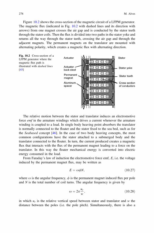
Figure 10.2 shows the cross-section of the magnetic circuit of a LFPM generator.The magnetic flux (indicated in Fig. 10.2 with dashed lines and its direction witharrows) from one magnet crosses the air gap and is conducted by the stator teeththrough the stator coils. Then the flux is divided into two paths in the stator yoke andreturns all the way through the stator teeth, crossing the air gap and through theadjacent magnets. The permanent magnets on the translator are mounted withalternating polarity, which creates a magnetic flux with alternating direction.

The relative motion between the stator and translator induces an electromotiveforce emf in the armature windings which drives a current whenever the armaturewinding is coupled to a load. In single body heaving point absorbers the translatoris normally connected to the floater and the stator fixed to the sea bed, such as forthe Seabased concept [46]. In the case of two body heaving concepts, the mostcommon configurations have the stator attached to a submerged body and thetranslator connected to the floater. In turn, the current produced creates a magneticflux that interacts with the flux of the permanent magnet leading to a force on thetranslator. In this way the floater mechanical energy is converted into electricenergy consumed in the load.

From Faraday’s law of induction the electromotive force emf, E, i.e. the voltageinduced by the permanent magnet flux, may be written as

E ¼ x/N; ð10:27Þ

where x is the angular frequency, / is the permanent magnet induced flux per poleand N is the total number of coil turns. The angular frequency is given by

x ¼ 2purw; ð10:28Þ

in which ur is the relative vertical speed between stator and translator and w thedistance between the poles (i.e. the pole pitch). Simultaneously, there is also a

Fig. 10.2 Cross-section of aLFPM generator where themagnetic flux path isillustrated with dashed lines[45]

278 M. Alves

resistive voltage drop in the slots, the end windings and cable connections when thegenerator is loaded. This resistive voltage drop per unit of length of the conductor isgiven by

E ¼ Iqcu; ð10:29Þ

where qcu is the resistivity of the conductor material (mostly copper) and I is thecurrent density in the conductor. As a result the induced phase currents produce amagnetic field, divided into two components: one component is coupled to theentire magnetic circuit, i.e. the main flux, and the other component is leakage flux.The corresponding inductances are then defined accordingly as the main induc-tance, Lm, and the leakage inductance, Ll. In a symmetric system the synchronousinductance, Ls, expressed in terms of the main inductance and the leakage induc-tance, is given by

Ls ¼ 32Lm þ Ll; ð10:30Þ

where the first term is the armature flux linkage with the phase winding, which willbe described below, and the second term is leakage inductance of that phase.

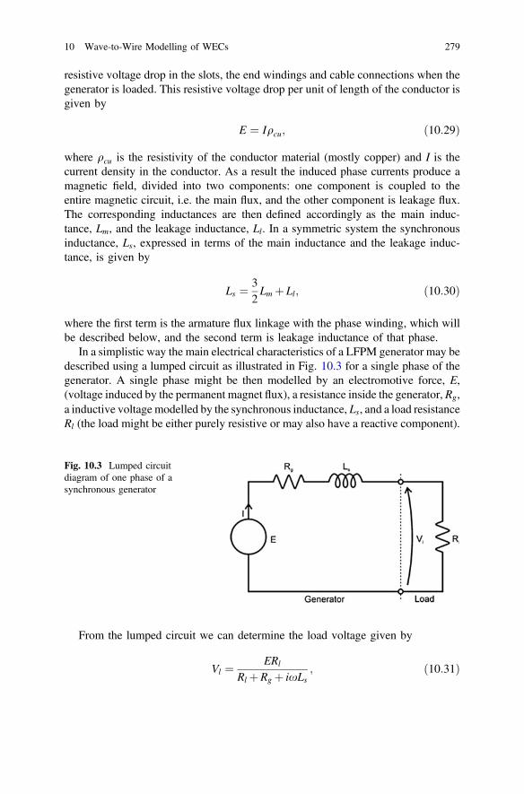
In a simplistic way the main electrical characteristics of a LFPM generator may bedescribed using a lumped circuit as illustrated in Fig. 10.3 for a single phase of thegenerator. A single phase might be then modelled by an electromotive force, E,(voltage induced by the permanent magnet flux), a resistance inside the generator, Rg,a inductive voltage modelled by the synchronous inductance, Ls, and a load resistanceRl (the load might be either purely resistive or may also have a reactive component).

From the lumped circuit we can determine the load voltage given by

Vl ¼ ERl

Rl þRg þ ixLs; ð10:31Þ

Fig. 10.3 Lumped circuitdiagram of one phase of asynchronous generator

10 Wave-to-Wire Modelling of WECs 279

the phase current by

I ¼ ERl þRg þ ixLs

; ð10:32Þ

and finally the power in the load is obtained from

P ¼ E2Rl

Rl þRg� �2 þ xLsð Þ2

: ð10:33Þ

Regardless of the type of electrical machine there are fundamentally two mainelectromagnetic forces: the normal force, attracting the two iron surfaces, and thethrust force, acting along the translator, in the longitudinal direction in linearmachines or tangential to the rotor surface in the case of rotating generators. Thecorresponding sheer, s, and normal, r, stresses are given respectively by

s ¼ BAe

2ð10:34Þ

and

r ¼ B2

2l0; ð10:35Þ

where B is the air gap magnetic flux density (the SI unit of magnetic flux density isthe Tesla, denoted by T), Ae is the electrical loading, measured in amperes per metre(A/m), and l0 the magnetic permeability of free space, also known as the magneticconstant, measured in henries per meter (H�m−1), or newton per ampere squared(NA−2). Typically the shear force density, Eq. 10.34, is limited in linear machines,since the air gap flux density is limited by saturation and cannot be increasedsubstantially in conventional machines. Moreover, the electrical loading is alsolimited because current loading produces heat, and heat dissipation is by and large adrawback in conventional machines. Heat dissipation can be increased to a certainextent by improving thermal design (e.g. water cooling system), but it would not beexpected to increase massively.

Besides the technical requirements for operating in irregular sea conditions withvery high peak forces and relatively low speeds, the design of LFPM generators hasa few additional complexities related to

(i) The design of the bearing system, which is quite intricate due to the highattractive force between translator and stator.

(ii) The mechanical construction with small air gaps. The stator construction ofLFPM generators is simple and robust, however typically the air gap betweenthe stator and the rotor has to be reasonably large, which reduces the air gapflux density and so the conversion efficiency. Essentially, the size of the gap

280 M. Alves

is imposed by manufacturing tolerances, the limited stiffness of the completeconstruction, large attractive forces between stator and translator, thermalexpansion, etc.

(iii) The power electronics converter to connect the WEC voltage (which hasvarying frequency and amplitude caused by the irregular motion and con-tinuously varying speed) to the electric grid (which has fixed frequency andamplitude).

(iv) The geometry of LFPM, however, limits the stator teeth width andcross-section area of the conductors for a given pole pitch. Increasing thetooth width to increase the magnetic flux in the stator or increasing theconductor cross-section demands a larger pole pitch and the angular fre-quency of the flux is thus reduced. This sets a limit for the induced emf perpole and consequently the power per air pat area.

10.2.7 End Stops Mechanism

End stops are mechanisms to restrict the stroke of the WEC moving bodies in orderto restrain the displacement within certain excursion limits for operational purposes,depending on the WEC working principle. End stops mechanisms are particularlyimportant in concepts operating at high velocities (e.g. heaving point absorbers).Virtual end stops may be incorporated in wave-to-wire models either as an inde-pendent additional force, representing a physical end stop, or included in thecontroller in order to avoid the bodies reaching the physical end stop, or to reducethe impact when limits are reached. Control methods for handling this kind of statesaturation problem consist of adding spring and/or damper (to dissipate excessivepower) terms to the calculation of the machinery force set-point. For instance, thisadditional force may be obtained from

Fes tð Þ ¼ Rm _g� sign _gð ÞKes gj j � glimð ÞH gj j � glimð Þ � Des _gu gj j � glimð Þ; ð10:36Þ

where H is the Heaviside step function and Kes and Des are the spring and dampingconstants for the end stop mechanism. The constant glim represents the excursion forwhich the mechanism starts acting [47].

10.3 Benchmark Analysis

This section presents a benchmark on existing wave-to-wire models and othermodeling tools, such as CFD codes, based on the Reynolds-AveragedNavier-Stokes equation (RANSE). At present CFD codes are not the most suit-able tools to model the entire chain of energy conversion (at least in a

10 Wave-to-Wire Modelling of WECs 281

Tab

le10

.1Benchmarkon

existin

gWECmod

elingtools

Developer

Codename

Fluid

mod

elHydro

model

Classes

ofWECs

PTO

mod

elMulti-bo

dyAccuracy

CPU

time

Seastates

Smallto

mod

erate

Mod

erateto

extrem

eSevere

DNV—GL1

Wavedyn

Perfect

fluid

LinearPF

TMoving

Bodies

Non

-linear

√+

+++

√X

X

Inno

sea2

Inwave

Perfect

fluid

Partially

nonlinearPF

TOWC

Moving

Bodies

Non

-linear

√++

++√

√X

ECN3

LAMSW

EC

Perfect

fluid

Partially

nonlinearPF

TMoving

Bodies

Non

-linear

X++

++√

√X

ECN

ACHIL3D

Perfect

fluid

LinearPF

TMoving

Bodies

Non

-linear

√+

+++

√X

X

Sand

ia/NREL4

WEC—

Sim

Perfect

fluid

LinearPF

TMoving

Bodies

Non

-linear

√+

+++

√X

X

Principia5

Diodo

rePerfect

fluid

LinearPF

TMoving

Bodies

Non

-linear

X+

+++

√X

X

WavEC6

WavEC2w

ire

Perfect

fluid

LinearPF

TOWC

Moving

Bodies

Non

-linear

√+

+++

√X

X

Marin

7Refresco

Viscous

fluid

RANSE

Moving

Bodies

N/A

√++

++

√√

√

ECN

Icare

Viscous

fluid

RANSE

Moving

Bodies

N/A

√++

++

√√

√

1 www.gl-garradhassan.com

2 www.in

nosea.fr

3 www.ec-nantes.fr

4 www.energy.sand

ia.gov

5 www.principia.fr

6 www.wavec.org

7 www.m

arin.nl

282 M. Alves

straightforward way) and evaluate different control strategies to enhance the deviceperformance. Nevertheless CFD codes might be extremely useful to study flowdetails of the wave-structure interaction (e.g. detection of flow separations, extremeloading and wave breaking).

The main differences between the codes listed in Table 10.1 reside in the theorythey are based on. For instance, modelling tools based on linear potential flowtheory (PFT) are not very time demanding (especially when compared with CFDcodes), although they allow the representation of a non-linear configuration of thePTO mechanism, which is the most realistic scenario for the majority of wavepower devices. However, these tools have a rather limited range of applicability andfairly low accuracy, largely due to the linear theory assumptions of small waves andsmall body motions.

Consequently, these limitations make the modelling tools based on linearpotential flow theory inadequate to assess WEC survival under extreme waveloading or even throughout operational conditions when the motion of the captor isnot of small amplitude. In order to overcome these limitations various modelsinclude some nonlinearities in the hydrodynamic wave-structure interaction. Themost common approach consists of computing the buoyancy and Froude-Krylovexcitation forces from the instantaneous position of a WEC device instead of fromits mean wet surface, as considered in the traditional linear hydrodynamic approach.The major advantage of these partially nonlinear codes is widening the range ofapplicability from intermediate to severe sea-states.

10.4 Radiation/Diffraction Codes

Usually wave-to-wire models rely on the output from 3D radiation/diffraction codes(such as ANSYS Aqwa [11], WAMIT [12], Moses [14] or the open source Nemohcode [13]), which are based on linear (and some of them second-order) potentialtheory for the analysis of submerged or floating bodies in the presence of oceanwaves. These sort of numerical tools use the boundary integral equation method(BIEM), also known as the panel method, to compute the velocity potential andfluid pressure on the body mean submerged surface (wetted surface in undisturbedconditions). Separate solutions for the diffraction problem, giving the effect ofthe incident waves on the body, and the radiation problems for each of the pre-scribed modes of motion of the bodies are obtained and then used to compute thehydrodynamic coefficients, where the most relevant are:

Added-Mass Coefficient:The added mass is the inertia added to a (partially or completely) submerged bodydue to the acceleration of the mass of the surrounding fluid as the body movesthrough it. The added-mass coefficient may be decomposed into two terms: afrequency dependent parameter which varies in accordance to the frequency of thesinusoidal oscillation of the body and a constant term, known as the infinite added

10 Wave-to-Wire Modelling of WECs 283

mass, which corresponds to the inertia added to the body when its oscillatorymotion does not radiate (generate) waves. This is the case when the body oscillateswith “infinite” frequency or when it is submerged very deep in the water.Damping Coefficient:In fluid dynamics the motion of an oscillatory body is damped by the resistive effectassociated with the waves generated by its motion. According to linear theory, thedamping force may be mathematically modelled as a force proportional to the bodyvelocity but opposite in direction, where the proportionality coefficient is calleddamping coefficient.Excitation force coefficient:According to linear theory the excitation coefficient is obtained by integrating thedynamic pressure exerted on the body’s mean wetted surface (undisturbed bodyposition) due to the action incident waves of unit amplitude, assuming that the bodyis stationary. The excitation coefficient results from adding to the integration of thepressure over the mean wetted body surface, caused by the incident wave in theabsence of the body (i.e. the pressure field undisturbed by the body presence), acorrection to the pressure field due to the body presence. This correction is obtainedby integrating the pressure over the mean wetted body surface caused by a scatteredwave owing to the presence of the body. The first term is known as theFroud-Krylov excitation and the second the scattered term.

10.5 Conclusion

Wave-to-wire models are extremely useful numerical tools for the study of thedynamic response of WECs in waves since they allow modelling of the entire chainof energy conversion from the wave-device hydrodynamic interaction to the elec-tricity feed into the electrical grid, with a considerable high level of accuracy andrelatively low CPU time. Wave-to-wire models allow the estimation of, amongother parameters, the motions/velocities/accelerations of the WEC captor, structuraland mooring loads, and the instantaneous power produced in irregular sea states.Therefore, these types of numerical tools are appropriate and widely used toevaluate the effectiveness of and to optimize control strategies.

Despite the usefulness of wave-to-wire models it is, however, important to bearin mind that they have some limitations that mostly arise from the linear wavetheory assumptions which are usually considered in modelling the hydrodynamicinteractions between ocean waves and WECs (e.g. linear waves, small responseamplitudes). Although these assumptions are fairly acceptable to model the oper-ational regime of WECs, which comprises small to moderate sea states, they are notappropriate to model the dynamic response of WECs under extreme conditions.Nevertheless, some sort of non-linear hydrodynamic modelling approaches mightbe included in wave to wire models (which extends the applicability of the model),such as the evaluation of the hydrostatic force at the instantaneous body position

284 M. Alves

instead of at its undisturbed position and/or the non-linear description of theFroud-Krylov term in the excitation force [48]. Ultimately, it is possible to trade offaccuracy and CPU time by choosing the partial non-linear hydrodynamic approachfor better accuracy, or the linear approach for faster computation.

Wave-to-wire models might be also used for modelling wave energy farmsinstead of single isolated devices. For this purpose the model must consider addi-tional forces on each device resulting from the waves radiated from the otherdevices in the wave farm. Obviously this hydrodynamic coupling effect signifi-cantly increases the CPU time. Some simplification may be considered for fastercomputation however, such as neglecting the effect of remote WECs, the radiationforce from which tends to be irrelevant when compared with that caused byneighbouring WECs. Moreover, the farm size and the hydrodynamic couplingbetween the WECs manifests an additional difficulty since it makes the applicationof BEM codes to generate the inputs required by wave-to-wire models (matrices ofhydrodynamic damping and added mass) more time consuming.

References

1. Ricci, P., Alves, M., Falcão, A., Sarmento, A.: Optimisation of the geometry of wave energyconverters. In: Proceedings of the OTTI International Conference on Ocean Energy (2006)

2. Pizer, D.: The numerical prediction of the performance of a solo duck, pp. 129–137. Eur.Wave Energy Symp., Edinburgh (1993)

3. Arzel, T., Bjarte-Larsson, T., Falnes J.: Hydrodynamic parameters for a floating wecforce-reacting against a submerged body. In: Proceedings of the 4th European Wave and TidalEnergy Conference (EWTEC), Denmark, pp. 267–274 (2000)

4. Structural Design of Wave Energy Devices (SDWED) project (international research alliancesupported by the Danish Council for Strategic Research) (2014). www.sdwed.civil.aau.dk/software

5. Losada, I.J., Lara, J.L., Guanche, R., Gonzalez-Ondina, J.M.: Numerical analysis of waveovertopping of rubble mound breakwaters. Coast. Eng. 55(1), 47–62 (2008)

6. www.aquaret.com7. Bogarino, B., Kofoed, J.P., Meinert, P.: Development of a Generic Power Simulation Tool for

Overtopping Based WEC, p. 35. Department of Civil Engineering, Aalborg University. DCETechnical Reports; No, Aalborg (2007)

8. Harris, R.E., Johanning, L.,Wolfram, J.: Mooring Systems for Wave Energy Converters: AReview of Design Issues and Choices. Heriot-Watt University, Edinburgh, UK (2004)

9. Structural Design of Wave Energy Devices (SDWED) project (international research alliancesupported by the Danish Council for Strategic Research), 2014. WP2—Moorings State of theart Copenhagen, 30 Aug 2010. www.sdwed.civil.aau.dk/

10. www.orcina.com11. www.ansys.com/Products/Other+Products/ANSYS+AQWA12. www.wamit.com13. www.ultramarine.com14. www.lheea.ec-nantes.fr/cgi-bin/hgweb.cgi/nemoh15. Jefferys, E., Broome, D., Patel, M.: A transfer function method of modelling systems with

frequency dependant coefficients. J. Guid. Control Dyn. 7(4), 490–494 (1984)16. Yu, Z., Falnes, J.: State-space modelling of a vertical cylinder in heave. Appl. Ocean Res. 17

(5), 265–275 (1995)

10 Wave-to-Wire Modelling of WECs 285

17. Schmiechen, M.: On state-space models and their application to hydrodynamic systems.NAUT Report 5002, Department of Naval Architecture, University of Tokyo, Japan (1973)

18. Kristansen, E., Egeland, O.: Frequency dependent added mass in models for controller designfor wave motion ship damping. In: Proceedings of the 6th IFAC Conference on Manoeuvringand Control of Marine Craft, Girona, Spain (2003)

19. Levy, E.: Complex curve fitting. IRE Trans. Autom. Control AC-4, 37–43 (1959)20. Sanathanan, C., Koerner, J.: Transfer function synthesis as a ratio of two complex

polynomials. IEEE Trnas. Autom., Control (1963)21. Perez, T., Fossen, T.: Time-domain vs. frequency-domain identification of parametric

radiation force models for marine structures at zero speed. Modell. Ident. Control 29(1), 1–19(2008)

22. Falnes, J.: Ocean Waves and Oscillating Systems. Book Cambridge University Press,Cambridge, UK (2002)

23. Budal, K., Falnes, J.: A resonant point absorber of ocean wave power. Nature 256, 478–479(1975)

24. Babarit, A., Duclos, G., Clement, A.H.: Comparison of latching control strategies for aheaving wave energy device in random sea. App. Ocean Energy 26, 227–238 (2004)

25. Falnes, J., Lillebekken P.M.: Budals latchingcontrolled-buoy type wavepower plant. In:Proceedings of the 5th European Wave and Tidal Energy Conference (EWTEC), Cork, Irland(2003)

26. Korde, U.A.: Latching control of deep water wave energy devices using an active reference.Ocean Eng. 29, 1343–1355 (2002)

27. Wright, A., Beattie, W.C., Thompson, A., Mavrakos, S.A., Lemonis, G., Nielsen, K., Holmes,B., Stasinopoulos, A.: Performance considerations in a power take off unit based on anon-linear load. In: Proceedings of the 5th European Wave and Tidal Energy Conference(EWTEC), Cork, Irland (2003)

28. Salter, S.H., Taylor, J.R.M., Caldwell, N.J.: Power conversion mechanisms for wave energy.In: Proceedings Institution of Mechanical Engineers Part M–J. of Engineering for the MaritimeEnvoronment, vol. 216, pp. 1–27 (2002)

29. Babarit, A., Guglielmi, M., Clement, A.H.: Declutching control of a wave energy converter.Ocean Eng. 36, 1015–1024 (2009)

30. Santos, M., Lafoz, M., Blanco, M., García-Tabarés, L., García, F., Echeandía, A., Gavela, L.:Testing of a full-scale PTO based on a switched reluctance linear generator for wave energyconversion. In: Proceedings of the 4th International Conference on Ocean Energy (ICOE),Dublin, Irland (2012)

31. Moretti G., Fontana M., Vertechy R.: Model-based design and optimization of a dielectricelastomer power take-off for oscillating wave surge energy converters. Meccanica. Submittedto the Special Issue on Soft Mechatronics (status: in review)

32. Falcão, A.F.: Modelling and control of oscillating body wave energy converters with hydraulicpower take-off and gas accumulator. Ocean Eng. 34, 2021–2032 (2007)

33. Gato, L.M.C., Falcao, A.F., Pereira, N.H.C, Pereira, R.J.: Design of wells turbine for OWCwave power plant. In: Procedings of the 1st International Offshore and Polar EngineeringConference, Edinburgh, UK (1991)

34. Setoguchi, T., Santhakumar, S., Takao, M., Kim, T.H., Kaneko, K.: A modified wells turbinefor wave energy conversion. Renew. Energy 28, 79–91 (2003)

35. Maeda, H., Santhakumar, S., Setoguchi, T., Takao, M., Kinoue, Y., Kaneko, K.: Performanceof an impulse turbine with fixed guide vanes for wave energy conversion. Renew. Energy 17,533–547 (1999)

36. Pereiras, B., Castro, F., El Marjani, A., Rodriguez, M.A.: An improved radial impulse turbinefor OWC. Renew. Energy 36(5), 1477–1484 (2011)

37. Falcão, A.F., Henriques, J.C.: Oscillating-water-column wave energy converters and airturbines: a review. Renew. Energy (2015). Online publication date: 1-Aug-2015

38. Evans, D.V.: The oscillating water column wave-energy device. J. Inst. Math. Appl. 22, 423–433 (1978)

286 M. Alves

39. Falcão, A.F., Justino, P.A.: OWC wave energy devices with air flow control. Ocean Eng. 26,1275–1295 (1999)

40. Dixon, S.L.: Fluid Mechanics and Thermodynamics of Turbomachinery, 4th edn. Butterworth,London (1998)

41. Polinder, H., Mueller, M.A., Scuotto, M., Sousa Prado, M.G.: Linear generator systems forwave energy conversion. In: Proceedings of the 7th European Wave and Tidal EnergyConference (EWTEC), Porto, Portugal (2007)

42. Polinder, H., Damen, M.E.C., Gardner, F.: Linear PM generator system for wave energyconversion in the AWS. IEEE Trans. Energy Convers. 19, 583–589 (2004)

43. Polinder, H., Mecrow, B.C., Jack, A.G., Dickinson, P., Mueller, M.A.: Linear generators fordirect drive wave energy conversion. IEEE Trans. Energy Convers. 20, 260–267 (2005)

44. Danielsson, O., Eriksson, M., Leijon, M.: Study of a longitudinal flux permanent magnet lineargenerator for wave energy converters. Int. J. Energy Res. in press, available online, WileyInterScience (2006)

45. Danielsson, O.: Wave energy conversion: linear synchronous permanent magnet generator.102p. (Digital Comprehensive Summaries of Uppsala Dissertations from the Faculty ofScience and Technology, 1651–6214; 232) (2006)

46. http://www.seabased.com/47. Hals, J., Falnes, J., Moan, T.: A comparison of selected strategies for adaptive control of wave

energy converters. J. Offshore Mech. Arct. Eng. 133(3), 031101 (2011)48. Gilloteaux, J.-C.: Mouvements de grande amplitude d’un corps flottant en fluide parfait.

Application à la récupération de l’énergie des vagues. Ph.D thesis, Ecole Centrale de Nantes;Université de Nantes. (in French) (2007)

Open Access This chapter is distributed under the terms of the Creative CommonsAttribution-Noncommercial 2.5 License (http://creativecommons.org/licenses/by-nc/2.5/) whichpermits any noncommercial use, distribution, and reproduction in any medium, provided theoriginal author(s) and source are credited.

The images or other third party material in this chapter are included in the work’s CreativeCommons license, unless indicated otherwise in the credit line; if such material is not included inthe work’s Creative Commons license and the respective action is not permitted by statutoryregulation, users will need to obtain permission from the license holder to duplicate, adapt orreproduce the material.

10 Wave-to-Wire Modelling of WECs 287