
Chapter 1 SVD, PCA & Pre- processing
33
Chapter 1 SVD, PCA & Pre- processing Part 3: Interpreting and computing the SVD
Transcript of Chapter 1 SVD, PCA & Pre- processing

Chapter 1 SVD, PCA & Pre-processing
Part 3: Interpreting and computing the SVD

DMM, summer 2015 Pauli Miettinen
Interpreting SVD
2Skillicorn chapter 3.2

DMM, summer 2015 Pauli Miettinen
Factor interpretation• Let A be objects-by-attributes and UΣVT its
SVD
• If two columns have similar values in a row of VT, these attributes are similar (have strong correlation)
• If two rows have similar values in a column of U, these objects are similar
3
DMM, summer 2015 Pauli Miettinen
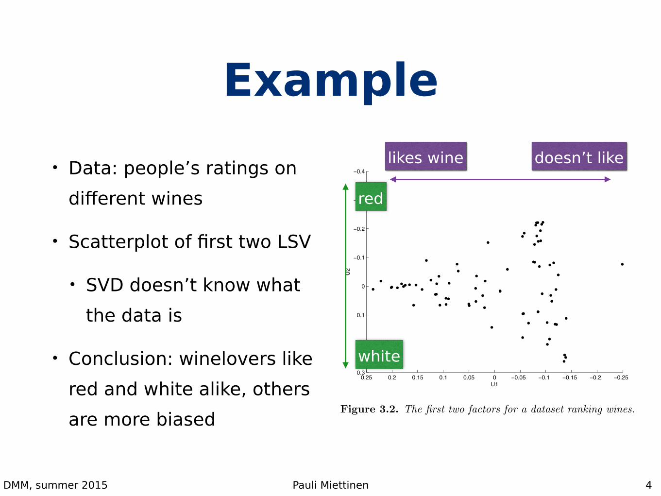
Example• Data: people’s ratings on
different wines
• Scatterplot of first two LSV
• SVD doesn’t know what the data is
• Conclusion: winelovers like red and white alike, others are more biased
4
3.2. Interpreting an SVD 55
−0.25−0.2−0.15−0.1−0.0500.050.10.150.20.25
−0.4
−0.3
−0.2
−0.1
0
0.1
0.2
0.3
U1
U2
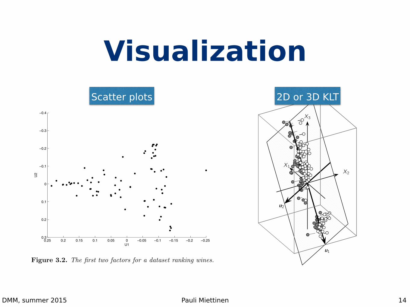
Figure 3.2. The first two factors for a dataset ranking wines.
plan, and medical insurance. It might turn out that all of these correlatestrongly with income, but it might not, and the differences in correlationmay provide insight into the contribution of a more general concept such as‘prosperity’ to happiness. The survey data can be put into a matrix withone row for each respondent, and one column for the response each question.An SVD of this matrix can help to find the latent factors behind the explicitfactors that each question and response is addressing.
For datasets of modest size, where the attributes exhibit strong correla-tions, this can work well. For example, Figure 3.2 is derived from a dataset inwhich 78 people were asked to rank 14 wines, from 1 to 14, although many didnot carry out a strict ranking. So the attributes in this dataset are wines, andthe entries are indications of how much each wine was liked by each person.The figure shows a plot along the first two axes of the transformed space,corresponding to the two most important factors. Some further analysis isrequired, but the first (most important) factor turns out to be liking for wine– those respondents at the left end of the plot are those who like wine, thatis who had many low numbers in their ‘ranking’, while those at the right endliked wine less across the board. This factor corresponds to something whichcould have been seen in the data relatively easily since it correlates stronglywith the sum of the ‘rankings’. For example, the outlier at the right endcorresponds to someone who rated every wine 14.
The second factor turns out to indicate preference for red versus whitewine – those respondents at the top of the plot prefer red wine over white,
© 2007 by Taylor and Francis Group, LLC
red
white
likes wine doesn’t like

DMM, summer 2015 Pauli Miettinen
Geometric interpretation• Let M = UΣVT
• Any linear mapping y=Mx can be expressed as a rotation, stretching, and rotation operation
• y1 = VTx is the first rotation
• y2 = Σy1 is the stretching
• y = Uy2 is the final rotation
5
DMM, summer 2015 Pauli Miettinen
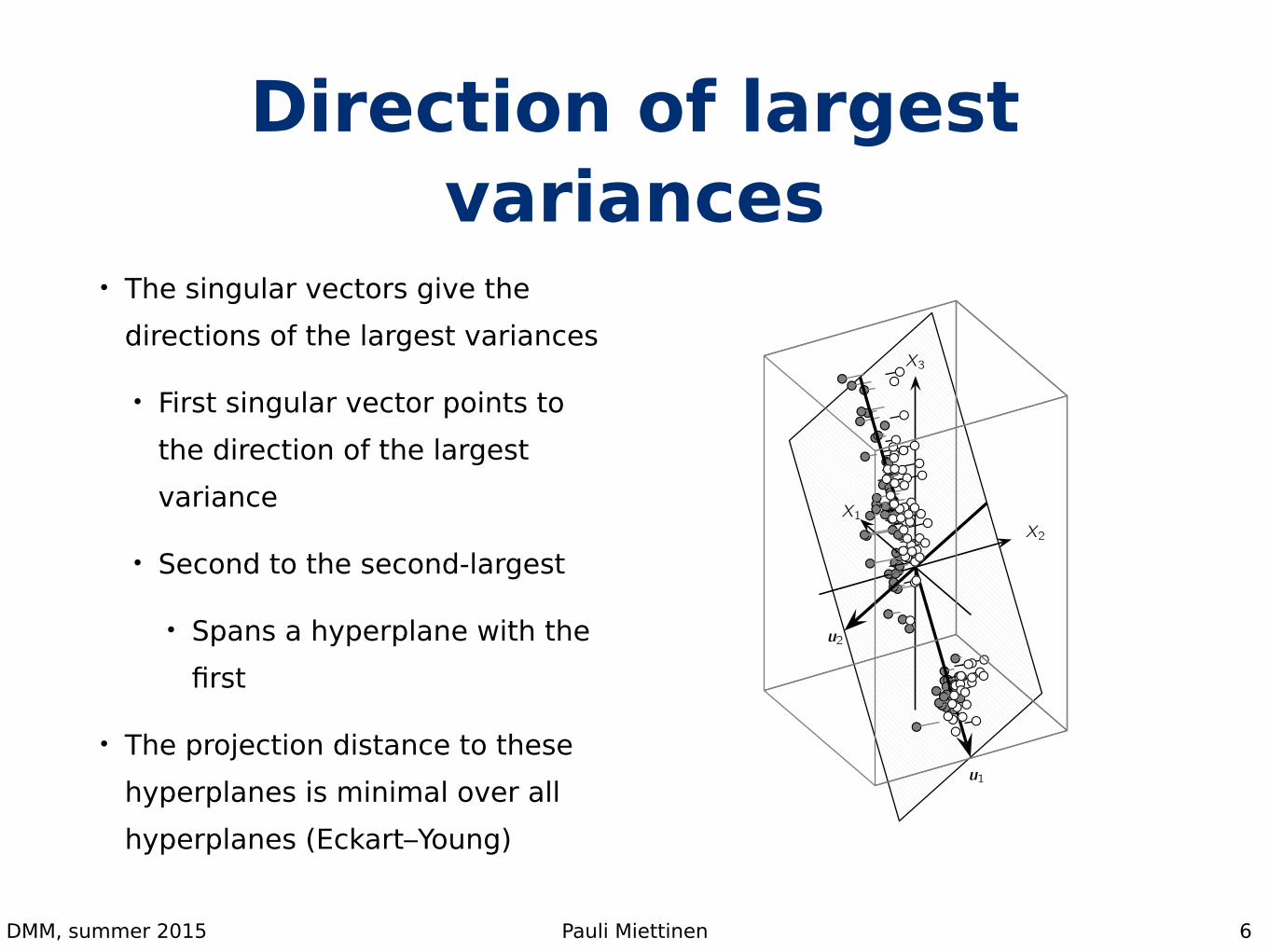
Direction of largest variances
• The singular vectors give the directions of the largest variances
• First singular vector points to the direction of the largest variance
• Second to the second-largest
• Spans a hyperplane with the first
• The projection distance to these hyperplanes is minimal over all hyperplanes (Eckart–Young)
6
IR&DM, WS'11/12 IX.1&2-17 January 2012
Example
34
CHAPTER 8. DIMENSIONALITY REDUCTION 173
X1X2
X3
(a) Original Basis: 3D
u1
u3
u2
(b) Optimal Basis: 3D
Figure 8.1: Iris Data: Optimal Basis
U matrix is an orthogonal matrix, whose columns, the basis vectors, are orthonormal,i.e., they are pairwise orthogonal and have unit length
uTi uj =
{1 if i = j
0 if i ̸= j(8.5)
Since U is orthogonal, this means that its inverse equals its transpose
U−1 = UT (8.6)
which implies that UTU = I, where I is the d × d identity matrix.Multiplying (8.3) on both sides by UT yields the expression for computing the
coordinates of x in the new basis
UT x = UTUa
a = UT x (8.7)
DRAFT @ 2011-11-10 09:03. Please do not distribute. Feedback is Welcome.Note that this book shall be available for purchase from Cambridge University Press and other standarddistribution channels, that no unauthorized distribution shall be allowed, and that the reader may makeone copy only for personal on-screen use.
IR&DM, WS'11/12 IX.1&2-17 January 2012
Example
34
CHAPTER 8. DIMENSIONALITY REDUCTION 180
variance uTΣΣΣu. Since we know that u1, the dominant eigenvector of ΣΣΣ maximizes theprojected variance, we have
MSE(u1) = var(D)− uT1 ΣΣΣu1 = var(D)− uT1 λ1u1 = var(D)− λ1
Thus, the principal component u1 which is the direction that maximizes the projectedvariance, is also the direction that minimizes the mean squared error.
X1X2
X3
u1
Figure 8.2: Best 1D or Line Approximation
Example 8.3: Figure 8.2 shows the first principal component, i.e., the best one di-mensional approximation, for the three dimensional Iris dataset shown in Figure 8.1a.The covariance matrix for this dataset is given as
ΣΣΣ =
⎛
⎜⎝0.681 −0.039 1.265−0.039 0.187 −0.3201.265 −0.320 3.092
⎞
⎟⎠
The largest eigenvalue is λ1 = 3.662, and the corresponding dominant eigenvectoris u1 = (−0.390, 0.089,−0.916)T . The unit vector u1 thus maximizes the projectedvariance, which is given as J(u1) = α = λ1 = 3.662. Figure 8.2 plots the principalcomponent u1. It also shows the error vectors ϵi , as thin gray line segments.
DRAFT @ 2011-11-10 09:03. Please do not distribute. Feedback is Welcome.Note that this book shall be available for purchase from Cambridge University Press and other standarddistribution channels, that no unauthorized distribution shall be allowed, and that the reader may makeone copy only for personal on-screen use.
IR&DM, WS'11/12 IX.1&2-17 January 2012
Example
34
CHAPTER 8. DIMENSIONALITY REDUCTION 184
X1X2
X3
u1
u2
(a) Optimal 2D Basis
X1X2
X3
(b) Non-Optimal 2D Basis
Figure 8.3: Best 2D Approximation
Example 8.4: For the Iris dataset from Example 8.1, the two largest eigenvalues areλ1 = 3.662, and λ2 = 0.239, with the corresponding eigenvectors
u1 =
⎛
⎜⎝−0.3900.089−0.916
⎞
⎟⎠ u2 =
⎛
⎜⎝−0.639−0.7420.200
⎞
⎟⎠
The projection matrix is given as
P2 = U2UT2 =
⎛
⎜⎝| |u1 u2| |
⎞
⎟⎠
(— uT1 —— uT2 —
)
= u1uT1 + u2u
T2
=
⎛
⎜⎝0.152 −0.035 0.357−0.035 0.008 −0.0820.357 −0.082 0.839
⎞
⎟⎠+
⎛
⎜⎝0.408 0.474 −0.1280.474 0.551 −0.148−0.128 −0.148 0.04
⎞
⎟⎠
=
⎛
⎜⎝0.560 0.439 0.2290.439 0.558 −0.2300.229 −0.230 0.879
⎞
⎟⎠
DRAFT @ 2011-11-10 09:03. Please do not distribute. Feedback is Welcome.Note that this book shall be available for purchase from Cambridge University Press and other standarddistribution channels, that no unauthorized distribution shall be allowed, and that the reader may makeone copy only for personal on-screen use.
DMM, summer 2015 Pauli Miettinen
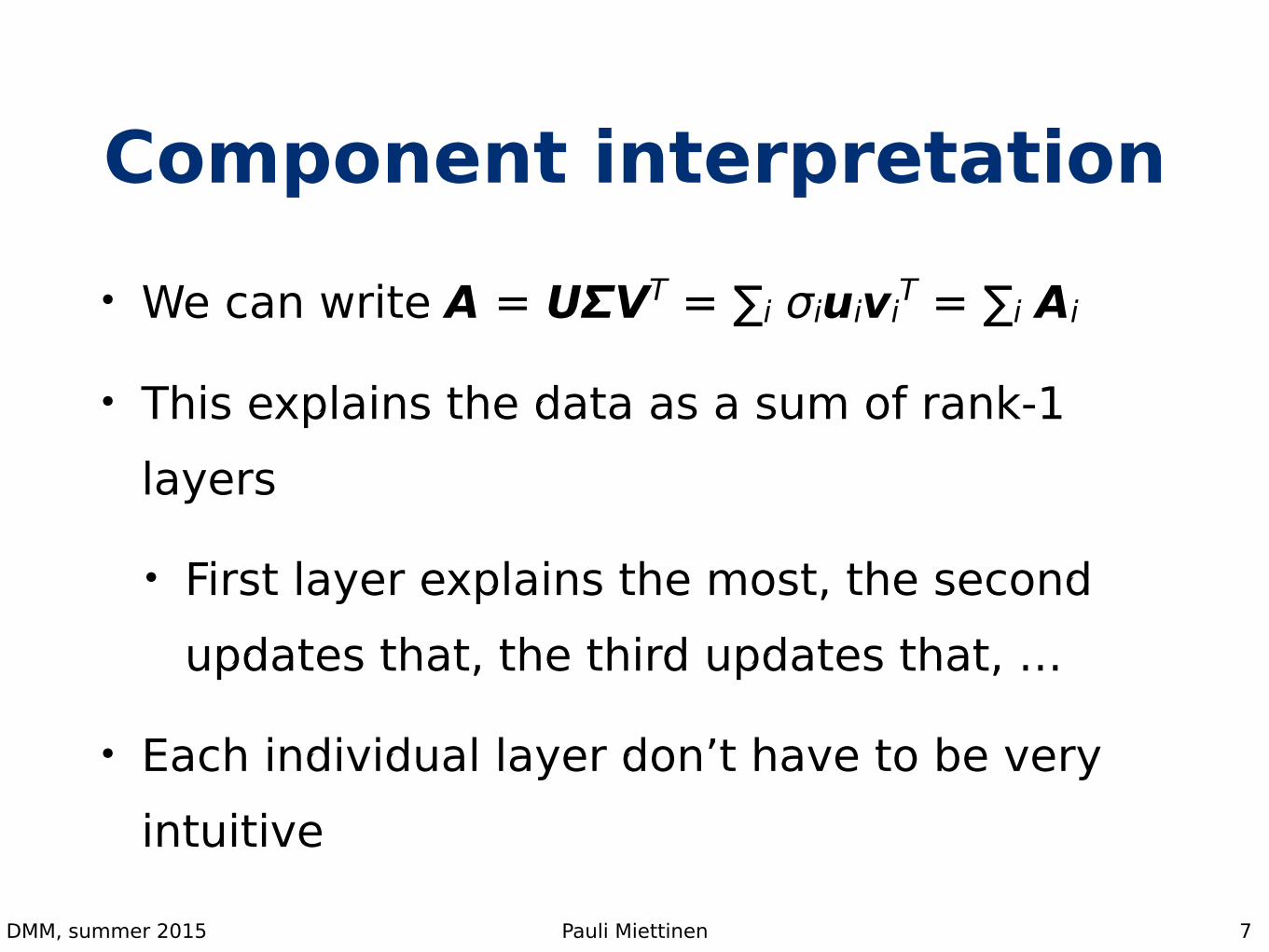
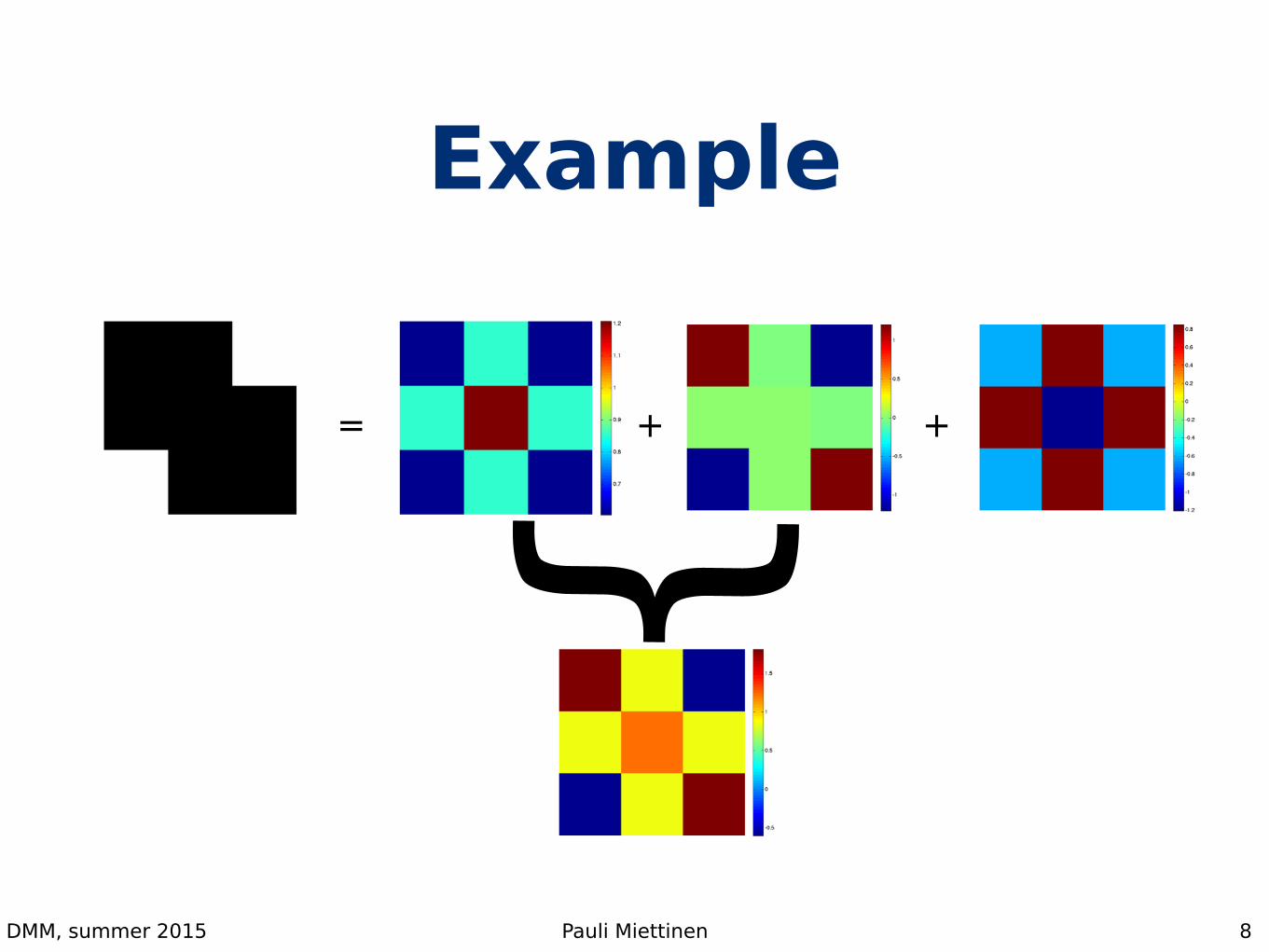
Component interpretation• We can write A = UΣVT = ∑i σiuivi
T = ∑i Ai
• This explains the data as a sum of rank-1 layers
• First layer explains the most, the second updates that, the third updates that, …
• Each individual layer don’t have to be very intuitive
7
DMM, summer 2015 Pauli Miettinen
Example
8
= + +
{
DMM, summer 2015 Pauli Miettinen
Applications of SVD
9Skillicorn chapter 3.5; Leskovec et al. chapter 11.3
DMM, summer 2015 Pauli Miettinen
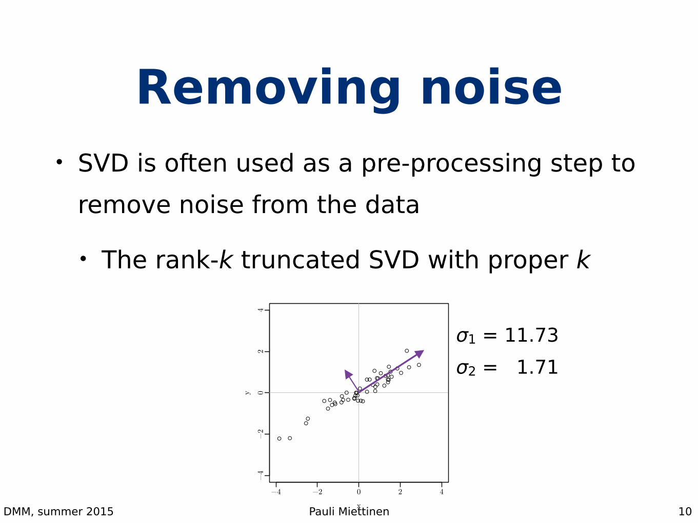
Removing noise• SVD is often used as a pre-processing step to
remove noise from the data
• The rank-k truncated SVD with proper k
10
−4 −2 0 2 4
−4
−2
02
4
x
y
● ●
●●
●
●●
●●● ●
●●
●
●
●●●
●●●
●
●
●
●●
●
●
●
●●●
●●
●
●
●
●
●●●●●
●
● ●●
●
●
●
σ1 = 11.73 σ2 = 1.71
DMM, summer 2015 Pauli Miettinen
Removing dimensions• SVD can be used to project the data to
smaller-dimensional subspace
• Original dimensions can have complex correlations
• Subsequent analysis is faster
• Points seem close to each other in high-dimensional space
11
Curse of dimensionality
DMM, summer 2015 Pauli Miettinen
Karhunen–Loève transform• The Karhunen–Loève transform (KLT) works as
follows:
• Normalize A ∈ ℝn×m to z-scores
• Compute the SVD UΣVT = A
• Project A ↦ AVk ∈ ℝn×k
• Vk = top-k right singular vectors
• A.k.a. the principal component analysis (PCA)
12
DMM, summer 2015 Pauli Miettinen
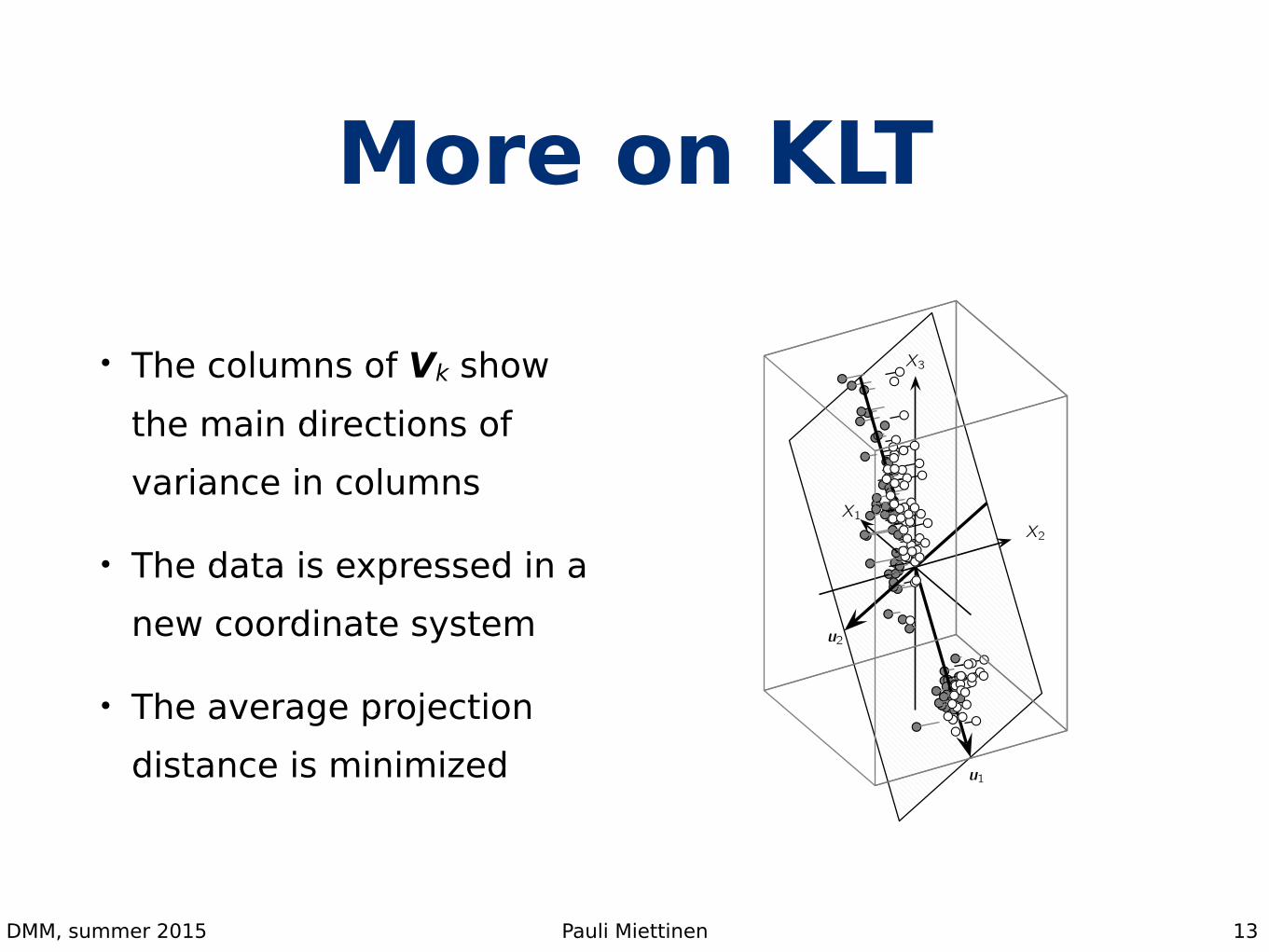
More on KLT
• The columns of Vk show the main directions of variance in columns
• The data is expressed in a new coordinate system
• The average projection distance is minimized
13
IR&DM, WS'11/12 IX.1&2-17 January 2012
Example
34
CHAPTER 8. DIMENSIONALITY REDUCTION 184
X1X2
X3
u1
u2
(a) Optimal 2D Basis
X1X2
X3
(b) Non-Optimal 2D Basis
Figure 8.3: Best 2D Approximation
Example 8.4: For the Iris dataset from Example 8.1, the two largest eigenvalues areλ1 = 3.662, and λ2 = 0.239, with the corresponding eigenvectors
u1 =
⎛
⎜⎝−0.3900.089−0.916
⎞
⎟⎠ u2 =
⎛
⎜⎝−0.639−0.7420.200
⎞
⎟⎠
The projection matrix is given as
P2 = U2UT2 =
⎛
⎜⎝| |u1 u2| |
⎞
⎟⎠
(— uT1 —— uT2 —
)
= u1uT1 + u2u
T2
=
⎛
⎜⎝0.152 −0.035 0.357−0.035 0.008 −0.0820.357 −0.082 0.839
⎞
⎟⎠+
⎛
⎜⎝0.408 0.474 −0.1280.474 0.551 −0.148−0.128 −0.148 0.04
⎞
⎟⎠
=
⎛
⎜⎝0.560 0.439 0.2290.439 0.558 −0.2300.229 −0.230 0.879
⎞
⎟⎠
DRAFT @ 2011-11-10 09:03. Please do not distribute. Feedback is Welcome.Note that this book shall be available for purchase from Cambridge University Press and other standarddistribution channels, that no unauthorized distribution shall be allowed, and that the reader may makeone copy only for personal on-screen use.
DMM, summer 2015 Pauli Miettinen
Visualization
14
IR&DM, WS'11/12 IX.1&2-17 January 2012
Example
34
CHAPTER 8. DIMENSIONALITY REDUCTION 184
X1X2
X3
u1
u2
(a) Optimal 2D Basis
X1X2
X3
(b) Non-Optimal 2D Basis
Figure 8.3: Best 2D Approximation
Example 8.4: For the Iris dataset from Example 8.1, the two largest eigenvalues areλ1 = 3.662, and λ2 = 0.239, with the corresponding eigenvectors
u1 =
⎛
⎜⎝−0.3900.089−0.916
⎞
⎟⎠ u2 =
⎛
⎜⎝−0.639−0.7420.200
⎞
⎟⎠
The projection matrix is given as
P2 = U2UT2 =
⎛
⎜⎝| |u1 u2| |
⎞
⎟⎠
(— uT1 —— uT2 —
)
= u1uT1 + u2u
T2
=
⎛
⎜⎝0.152 −0.035 0.357−0.035 0.008 −0.0820.357 −0.082 0.839
⎞
⎟⎠+
⎛
⎜⎝0.408 0.474 −0.1280.474 0.551 −0.148−0.128 −0.148 0.04
⎞
⎟⎠
=
⎛
⎜⎝0.560 0.439 0.2290.439 0.558 −0.2300.229 −0.230 0.879
⎞
⎟⎠
DRAFT @ 2011-11-10 09:03. Please do not distribute. Feedback is Welcome.Note that this book shall be available for purchase from Cambridge University Press and other standarddistribution channels, that no unauthorized distribution shall be allowed, and that the reader may makeone copy only for personal on-screen use.
3.2. Interpreting an SVD 55
−0.25−0.2−0.15−0.1−0.0500.050.10.150.20.25
−0.4
−0.3
−0.2
−0.1
0
0.1
0.2
0.3
U1
U2
Figure 3.2. The first two factors for a dataset ranking wines.
plan, and medical insurance. It might turn out that all of these correlatestrongly with income, but it might not, and the differences in correlationmay provide insight into the contribution of a more general concept such as‘prosperity’ to happiness. The survey data can be put into a matrix withone row for each respondent, and one column for the response each question.An SVD of this matrix can help to find the latent factors behind the explicitfactors that each question and response is addressing.
For datasets of modest size, where the attributes exhibit strong correla-tions, this can work well. For example, Figure 3.2 is derived from a dataset inwhich 78 people were asked to rank 14 wines, from 1 to 14, although many didnot carry out a strict ranking. So the attributes in this dataset are wines, andthe entries are indications of how much each wine was liked by each person.The figure shows a plot along the first two axes of the transformed space,corresponding to the two most important factors. Some further analysis isrequired, but the first (most important) factor turns out to be liking for wine– those respondents at the left end of the plot are those who like wine, thatis who had many low numbers in their ‘ranking’, while those at the right endliked wine less across the board. This factor corresponds to something whichcould have been seen in the data relatively easily since it correlates stronglywith the sum of the ‘rankings’. For example, the outlier at the right endcorresponds to someone who rated every wine 14.
The second factor turns out to indicate preference for red versus whitewine – those respondents at the top of the plot prefer red wine over white,
© 2007 by Taylor and Francis Group, LLC
Scatter plots 2D or 3D KLT
DMM, summer 2015 Pauli Miettinen
Latent Semantic Analysis & Indexing
• Latent semantic analysis (LSA) is a latent topic model
• Documents-by-terms matrix A
• Typically normalized (e.g. tf/idf)
• Goal is to find the “topics” doing SVD
• U associates documents to topics
• V associates topics to terms
• Queries can be answered by projecting the query vector q to q’ = qVΣ–1 and returning rows of U that are similar to q’
15
DMM, summer 2015 Pauli Miettinen
And many more…
• Determining the rank, finding the least-squares solution, recommending the movies, ordering results of queries, …
16

DMM, summer 2015 Pauli Miettinen
Computing the SVD
17Golub & Van Loan chapters 5.1, 5.4.8, and 8.6
DMM, summer 2015 Pauli Miettinen
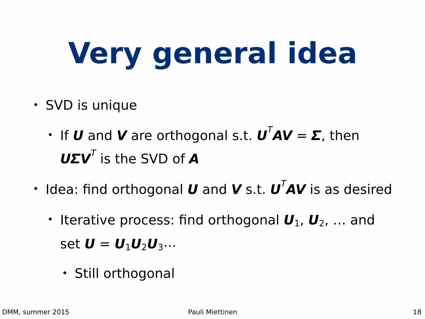
Very general idea• SVD is unique
• If U and V are orthogonal s.t. UTAV = Σ, then UΣVT is the SVD of A
• Idea: find orthogonal U and V s.t. UTAV is as desired
• Iterative process: find orthogonal U1, U2, … and set U = U1U2U3…
• Still orthogonal
18
DMM, summer 2015 Pauli Miettinen
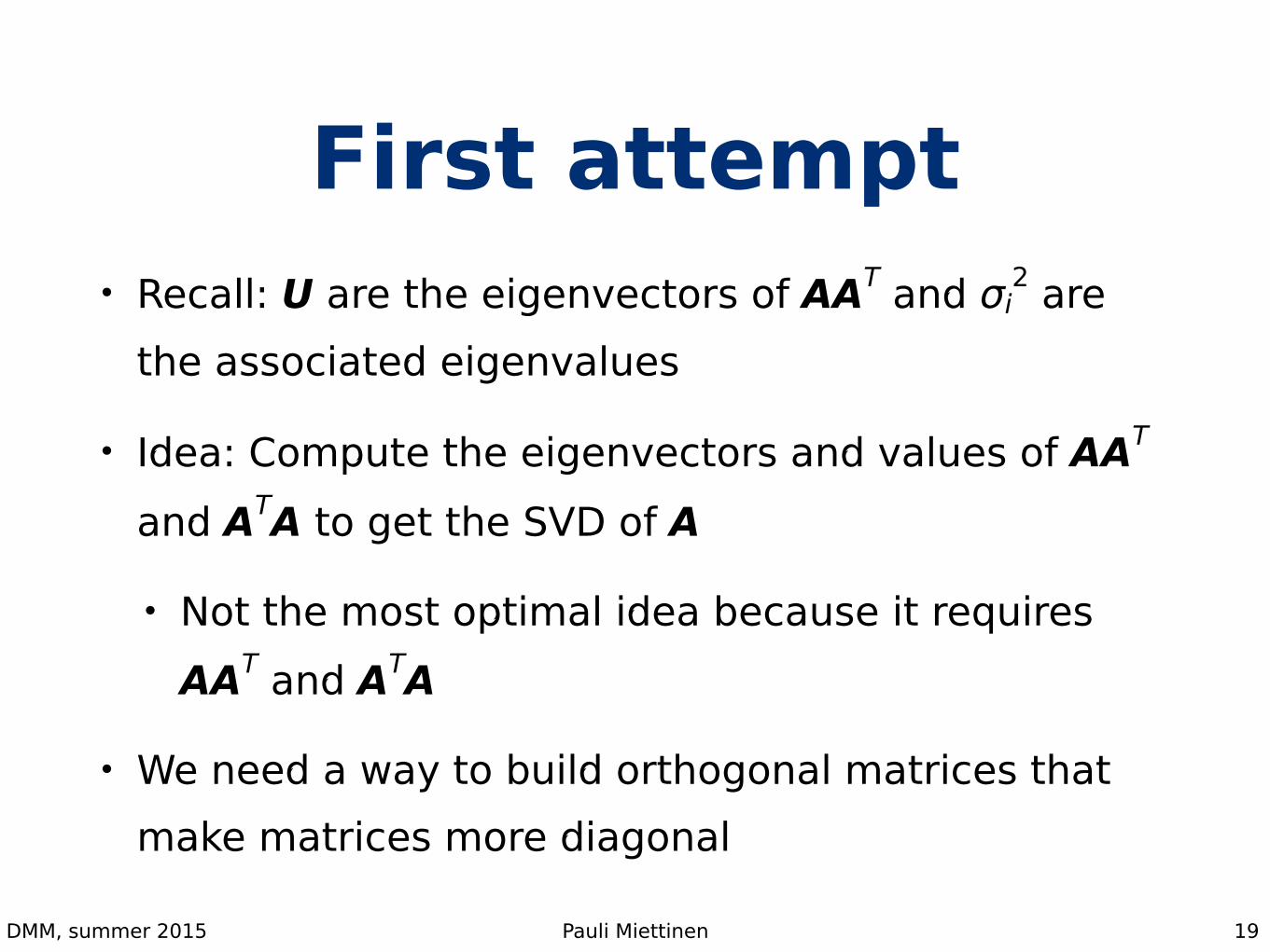
First attempt• Recall: U are the eigenvectors of AAT and σi
2 are the associated eigenvalues
• Idea: Compute the eigenvectors and values of AAT and ATA to get the SVD of A
• Not the most optimal idea because it requires AAT and ATA
• We need a way to build orthogonal matrices that make matrices more diagonal
19
DMM, summer 2015 Pauli Miettinen
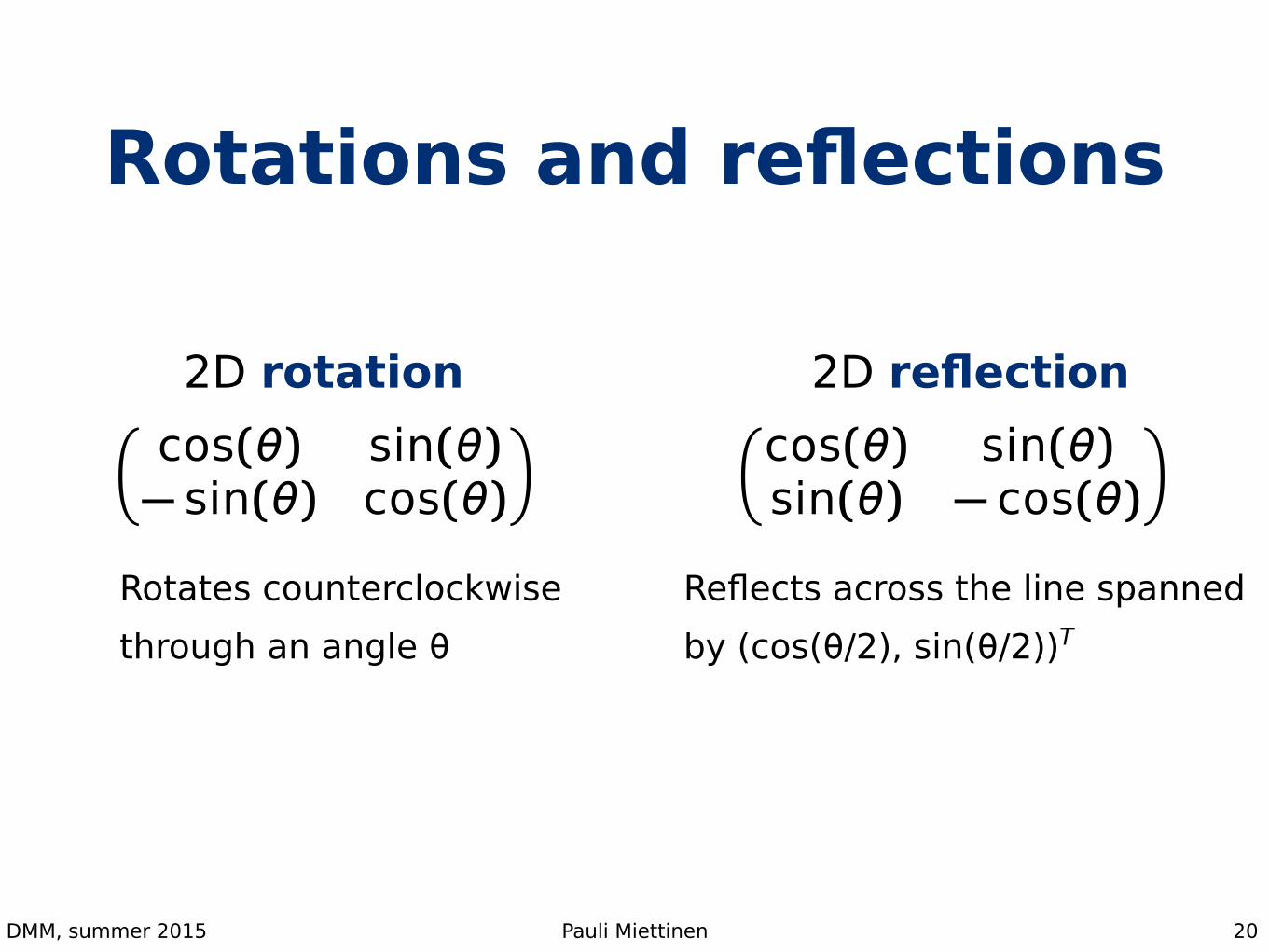
Rotations and reflections
20
Åcos(�) sin(�)� sin(�) cos(�)
ã Åcos(�) sin(�)sin(�) � cos(�)
ã2D rotation 2D reflection
Rotates counterclockwise through an angle θ
Reflects across the line spanned by (cos(θ/2), sin(θ/2))T

DMM, summer 2015 Pauli Miettinen
Example
21
x = (√2, √2)TQ =Åcos(�/4) sin(�/4)� sin(�/4) cos(�/4)
ã
Qx = (2, 0)T
This coordinate is now 0!

DMM, summer 2015 Pauli Miettinen
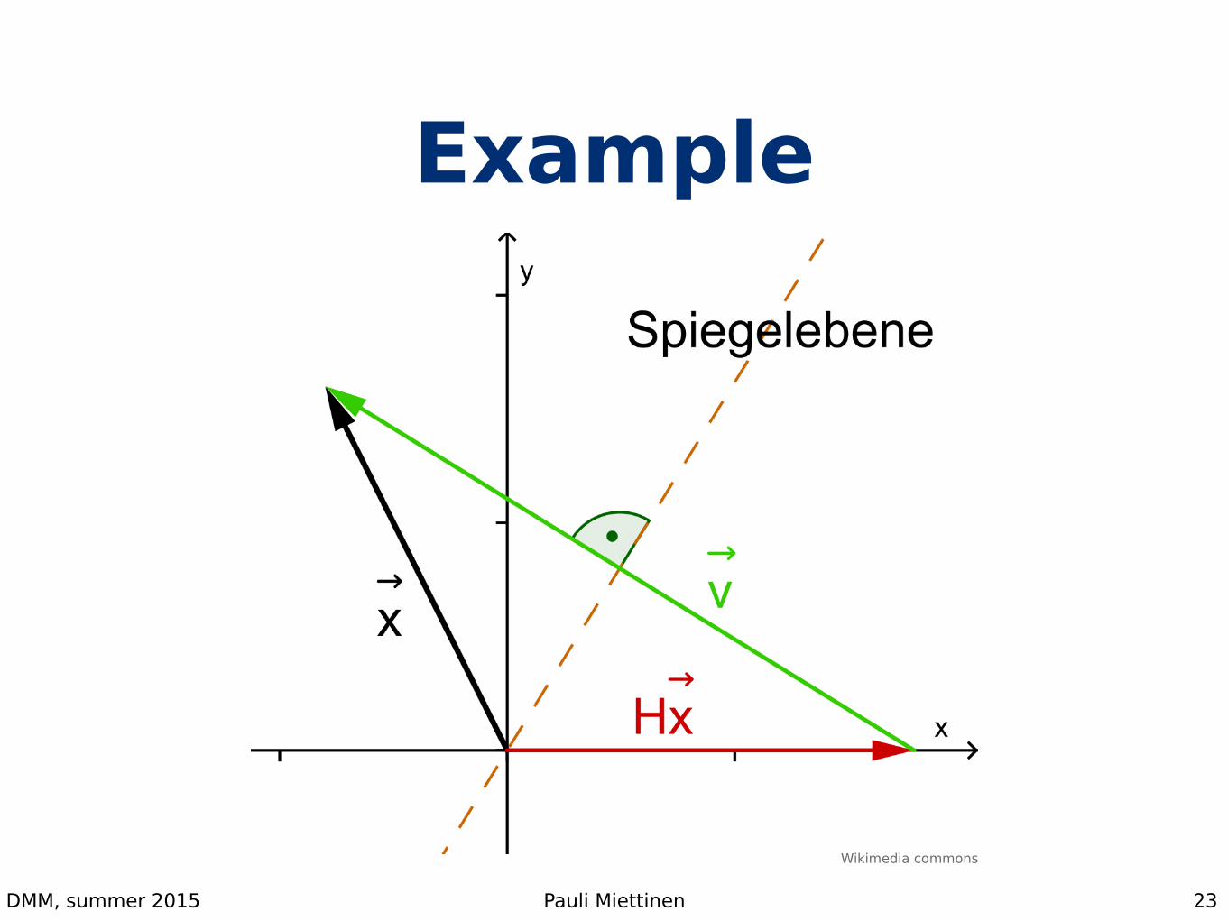
Householder reflections• A Householder reflection is n-by-n matrix
• If we set v = x – ||x||2e1, then Px = ||x||2e1
• e1 = (1, 0, 0, …, 0)T
• Note: PA = A – (βv)(vTA) where β = 2/(vTv)
• We never have to compute matrix P
22
P = � � ���T where � =2
�T�
DMM, summer 2015 Pauli Miettinen
Example
23
Wikimedia commons
DMM, summer 2015 Pauli Miettinen
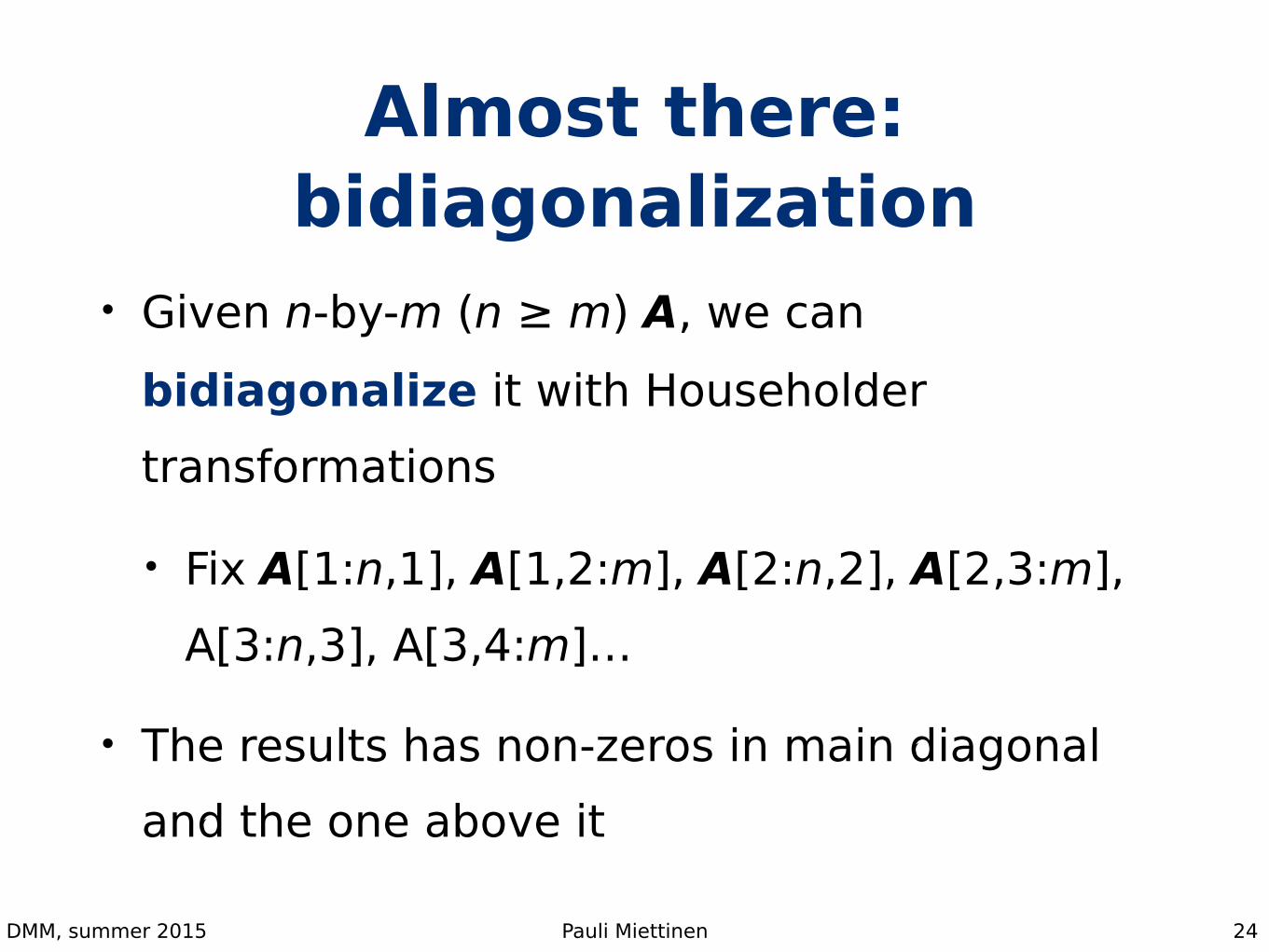
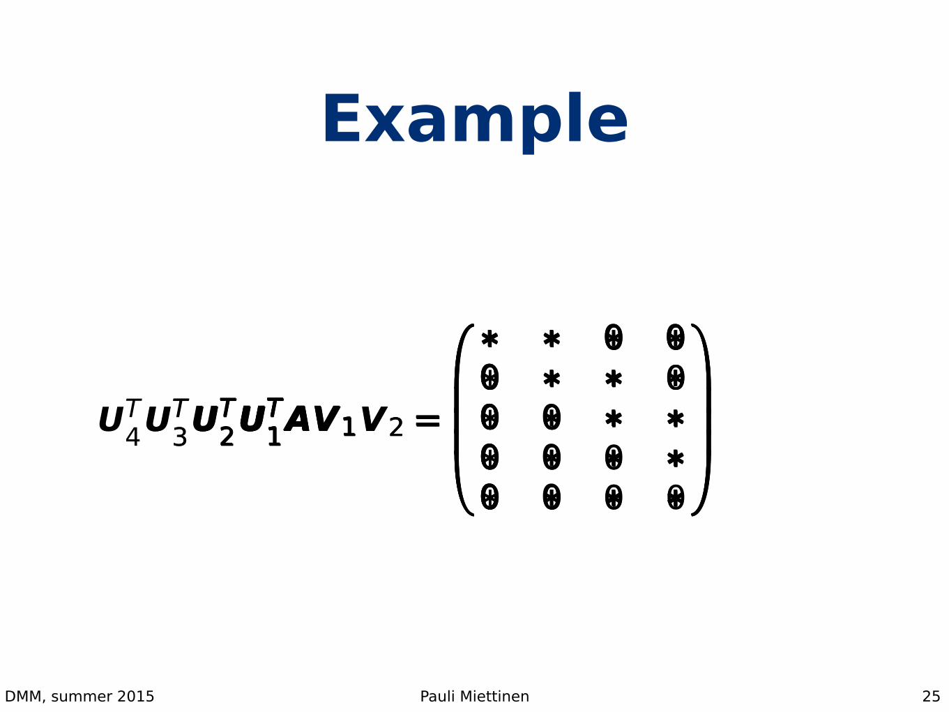
Almost there: bidiagonalization
• Given n-by-m (n ≥ m) A, we can bidiagonalize it with Householder transformations
• Fix A[1:n,1], A[1,2:m], A[2:n,2], A[2,3:m], A[3:n,3], A[3,4:m]…
• The results has non-zeros in main diagonal and the one above it
24
DMM, summer 2015 Pauli Miettinen
Example
25
A =
0BBB@
� � � �� � � �� � � �� � � �� � � �
1CCCAUT
1A =
0BBB@
� � � �0 � � �0 � � �0 � � �0 � � �
1CCCAUT
1AV1 =
0BBB@
� � 0 00 � � �0 � � �0 � � �0 � � �
1CCCAUT
2UT1AV1 =
0BBB@
� � 0 00 � � �0 0 � �0 0 � �0 0 � �
1CCCAUT
2UT1AV1V2 =
0BBB@
� � 0 00 � � 00 0 � �0 0 � �0 0 � �
1CCCAUT
3UT2U
T1AV1V2 =
0BBB@
� � 0 00 � � 00 0 � �0 0 0 �0 0 0 �
1CCCAUT
4UT3U
T2U
T1AV1V2 =
0BBB@
� � 0 00 � � 00 0 � �0 0 0 �0 0 0 0
1CCCA
DMM, summer 2015 Pauli Miettinen
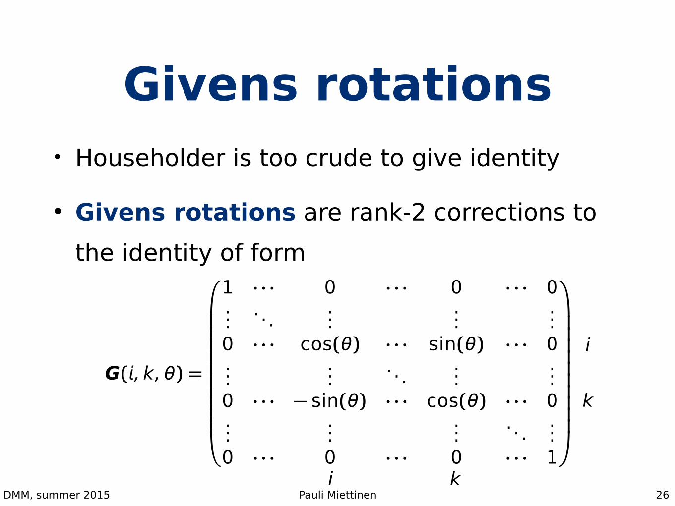
Givens rotations• Householder is too crude to give identity
• Givens rotations are rank-2 corrections to the identity of form
26
G(�, k,�) =
0BBBBBBBBBB@
1 · · · 0 · · · 0 · · · 0...
. . ....
......
0 · · · cos(�) · · · sin(�) · · · 0...
.... . .
......
0 · · · � sin(�) · · · cos(�) · · · 0...
......
. . ....
0 · · · 0 · · · 0 · · · 1
1CCCCCCCCCCA
i k
i
k

DMM, summer 2015 Pauli Miettinen
Applying Givens• Set θ s.t.
and
• Now
• N.B. G(i, k, θ)TA only affects to the 2 rows A[c(i, k),]
• Also, no inverse trig. operations are needed
27
cos(�) = ��«�2� +�
2k
sin(�) = ��k«�2� +�
2k
Åcos(�) sin(�)� sin(�) cos(�)
ãT Å���k
ã=År0
ã
DMM, summer 2015 Pauli Miettinen
Givens in SVD• We use Givens transformations to erase the
superdiagonal
• Consider principal 2-by-2 submatrices A[k:k+1,k:k+1]
• Rotations can introduce unwanted non-zeros to A[k+2,k] (or A[k,k+2])
• Fix them in the next sub-matrix
28
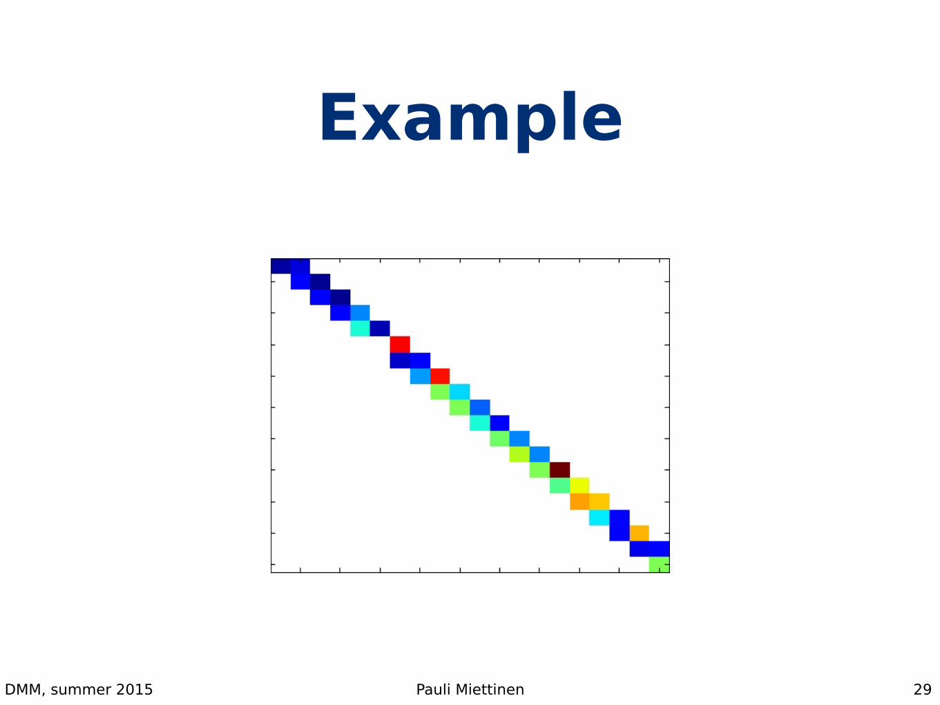
DMM, summer 2015 Pauli Miettinen
Example
29
DMM, summer 2015 Pauli Miettinen
Putting it all together
1. Compute the bidiagonal matrix B from A using Householder transformations
2. Apply the Givens rotations to B until it is fully diagonal
3. Collect the required results
30
DMM, summer 2015 Pauli Miettinen
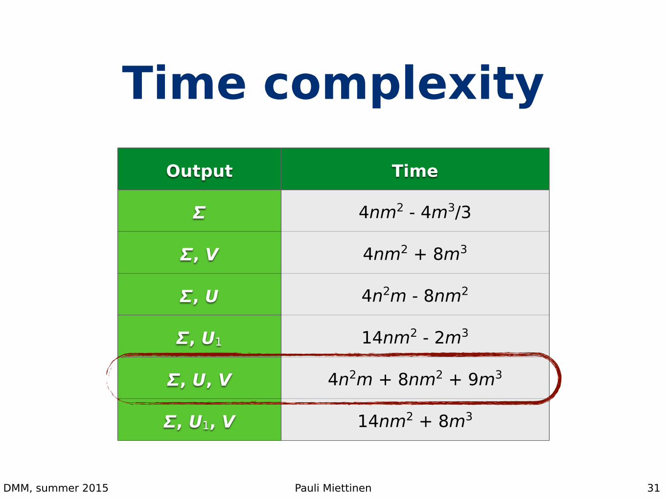
Time complexity
31
Output Time
Σ 4nm2 - 4m3/3
Σ, V 4nm2 + 8m3
Σ, U 4n2m - 8nm2
Σ, U1 14nm2 - 2m3
Σ, U, V 4n2m + 8nm2 + 9m3
Σ, U1, V 14nm2 + 8m3
DMM, summer 2015 Pauli Miettinen
Summary of computing SVD
• Rotations and reflections allow us to selectively zero elements of a matrix with orthogonal transformations
• Used in many, many decompositions
• Fast and accurate results require careful implementations
• Other techniques are faster for truncated SVD in large, sparse matrices
32
DMM, summer 2015 Pauli Miettinen
Summary of SVD• Truly the workhorse of numerical linear algebra
• Many useful theoretical properties
• Rank-revealing, pseudo-inverses, scalar norm computation, …
• Reasonably easy to compute
• But it also has some major shortcomings in data analysis… stay tuned!
33


![Nonstationary Dynamics Data Analysis With Wavelet-SVD ...ity, and harmonic wavelet properties [23, 24]. This paper augments time-frequency multiscale wavelet processing with SVD filtering](https://static.fdocuments.in/doc/165x107/5eb46f4794d6bd2220028872/nonstationary-dynamics-data-analysis-with-wavelet-svd-ity-and-harmonic-wavelet.jpg)


![[Marc Moonen] SVD and Signal Processing III Algor(BookFi.org)](https://static.fdocuments.in/doc/165x107/5529ff984a79590e778b4640/marc-moonen-svd-and-signal-processing-iii-algorbookfiorg.jpg)
