Chapter 1 STERN-GERLACH EXPERIMENTSdepts.washington.edu/jrphys/ph248A11/qmch1.pdf · Chap. 1...

8/10/10 1-1

Chapter 1 STERN-GERLACH EXPERIMENTS

It was not a dark and stormy night when Otto Stern and Walther Gerlach

performed their now famous experiment in 1922. The Stern-Gerlach experiment

demonstrated that measurements on microscopic or quantum particles are not always as

certain as we might expect. Quantum particles behave as mysteriously as Erwin's

socks—sometimes forgetting what we have already measured. Erwin's adventure with

the mystery socks is farfetched because you know that everyday objects do not behave

like his socks. If you observe a sock to be black, it remains black no matter what other

properties of the sock you observe. However, the Stern-Gerlach experiment goes against

these ideas. Microscopic or quantum particles do not behave like the classical objects of

your everyday experience. The act of observing a quantum particle affects its measurable

properties in a way that is foreign to our classical experience.

In these first three chapters, we focus on the Stern-Gerlach experiment because it

is a conceptually simple experiment that demonstrates many basic principles of quantum

mechanics. We discuss a variety of experimental results and the quantum theory that has

been developed to predict those results. The mathematical formalism of quantum

mechanics is based upon six postulates that we will introduce as we develop the

theoretical framework. (A complete list of these postulates is in Section 1.5.) We use the

Stern-Gerlach experiment to learn about quantum mechanics theory for two primary

reasons: (1) It demonstrates how quantum mechanics works in principle by illustrating

the postulates of quantum mechanics, and (2) It demonstrates how quantum mechanics

works in practice through the use of Dirac notation and matrix mechanics to solve

problems. By using a simple example, we can focus on the principles and the new

mathematics, rather than having the complexity of the physics obscure these new aspects.

1.1 Stern-Gerlach experiment

In 1922 Otto Stern and Walther Gerlach performed a seminal experiment in the

history of quantum mechanics. In its simplest form, the experiment consists of an oven

that produces a beam of neutral atoms, a region of space with an inhomogeneous

magnetic field, and a detector for the atoms, as depicted in Fig. 1.1. Stern and Gerlach

used a beam of silver atoms and found that the beam was split into two in its passage

through the magnetic field. One beam was deflected upwards and one downwards in

relation to the direction of the magnetic field gradient.

To understand why this result is so at odds with our classical expectations, we

must first analyze the experiment classically. The results of the experiment suggest an

interaction between a neutral particle and a magnetic field. We expect such an

interaction if the particle possesses a magnetic moment µ . The potential energy of this

interaction is E = !µiB , which results in a force

F = ! µiB( ) . In the Stern-Gerlach

experiment, the magnetic field gradient is primarily in the z-direction, and

Chap. 1 Stern-Gerlach Experiments

8/10/10

1-2

Figure 1.1 Stern-Gerlach experiment to measure the spin component of neutral particles along

the z-axis. The magnetic cross-section at right shows the inhomogeneous field used in the experiment.

the resulting z-component of the force is

Fz=

!

!zµiB( )

" µz

!Bz

!z

. (1.1)

This force is perpendicular to the direction of motion and deflects the beam in proportion

to the component of the magnetic moment in the direction of the magnetic field gradient.

Now consider how to understand the origin of the atom's magnetic moment from

a classical viewpoint. The atom consists of charged particles, which, if in motion, can

produce loops of current that give rise to magnetic moments. A loop of area A and

current I produces a magnetic moment

µ = IA (1.2)

in MKS units. If this loop of current arises from a charge q traveling at speed v in a circle

of radius r, then

µ =q

2!r v!r

2

=qrv

2

=q

2mL

, (1.3)

where L = mrv is the orbital angular momentum of the particle. In the same way that the

earth revolves around the sun and rotates around its own axis, we can also imagine a

charged particle in an atom having orbital angular momentum L and a new property,

the intrinsic angular momentum, which we label S and call spin. The intrinsic angular

momentum also creates current loops, so we expect a similar relation between the

magnetic moment µ and S. The exact calculation involves an integral over the charge


8/10/10

1-3

distribution, which we will not do. We simply assume that we can relate the magnetic

moment to the intrinsic angular momentum in the same fashion as Eq. (1.3), giving

µ = gq

2mS , (1.4)

where the dimensionless gyroscopic ratio g contains the details of that integral.

A silver atom has 47 electrons, 47 protons, and 60 or 62 neutrons (for the most

common isotopes). The magnetic moments depend on the inverse of the particle mass, so

we expect the heavy protons and neutrons (! 2000 me) to have little effect on the

magnetic moment of the atom and so we neglect them. From your study of the periodic

table in chemistry, you recall that silver has an electronic configuration

1s22s

22p63s

23p64s

23d104p

64d105s

1, which means that there is only the lone 5s electron

outside of the closed shells. The electrons in the closed shells can be represented by a

spherically symmetric cloud with no orbital or intrinsic angular momentum

(unfortunately we are injecting some quantum mechanical knowledge of atomic physics

into this classical discussion). That leaves the lone 5s electron as a contributor to the

magnetic moment of the atom as a whole. An electron in an s state has no orbital angular

momentum, but it does have spin. Hence the magnetic moment of this electron, and

therefore of the entire neutral silver atom, is

µ = !ge

2me

S , (1.5)

where e is the magnitude of the electron charge. The classical force on the atom can now

be written as

Fz ! "ge

2me

Sz#Bz

#z. (1.6)

The deflection of the beam in the Stern-Gerlach experiment is thus a measure of the

component (or projection) Sz of the spin along the z-axis, which is the orientation of the

magnetic field gradient.

If we assume that the 5s electron of each atom has the same magnitude S of the

intrinsic angular momentum or spin, then classically we would write the z-component as

Sz= S cos! , where ! is the angle between the z-axis and the direction of the spin S. In

the thermal environment of the oven, we expect a random distribution of spin directions

and hence all possible angles !. Thus we expect some continuous distribution (the details

are not important) of spin components from Sz= ! S to S

z= + S , which would yield a

continuous spread in deflections of the silver atomic beam. Rather, the experimental

result that Stern and Gerlach observed was that there are only two deflections, indicating

that there are only two possible values of the z-component of the electron spin. The

magnitudes of these deflections are consistent with values of the spin component of

Sz= ±!

2, (1.7)


8/10/10

1-4

where ! is Planck's constant h divided by 2! and has the numerical value

! = 1.0546 !10"34J #s

=!6.5821!10"16eV #s

. (1.8)

This result of the Stern-Gerlach experiment is evidence of the quantization of the

electron's spin angular momentum component along an axis. This quantization is at odds

with our classical expectations for this measurement. The factor of 1/2 in Eq. (1.7) leads

us to refer to this as a spin 1/2 system.

In this example, we have chosen the z-axis along which to measure the spin

component, but there is nothing special about this direction in space. We could have

chosen any other axis and we would have obtained the same results.

Now that we know the fine details of the Stern-Gerlach experiment, we simplify

the experiment for the rest of our discussions by focusing on the essential features. A

simplified schematic representation of the experiment is shown in Fig. 1.2, which depicts

an oven that produces the beam of atoms, a Stern-Gerlach device with two output ports

for the two possible values of the spin component, and two counters to detect the atoms

leaving the output ports of the Stern-Gerlach device. The Stern-Gerlach device is labeled

with the axis along which the magnetic field is oriented. The up and down arrows

indicate the two possible measurement results for the device; they correspond

respectively to the results Sz= ±! 2 in the case where the field is oriented along the

z-axis. There are only two possible results in this case, so they are generally referred to

as spin up and spin down. The physical quantity that is measured, Sz in this case, is

called an observable. In our detailed discussion of the experiment above, we chose the

field gradient in such a manner that the spin up states were deflected upwards. In this

new simplification, the deflection itself is not an important issue. We simply label the

output port with the desired state and count the particles leaving that port. The Stern-

Gerlach device sorts (or filters or selects or analyzes) the incoming particles into the two

possible outputs Sz= ±! 2 in the same way that Erwin sorted his socks according to

color or length. We follow convention and refer to a Stern-Gerlach device as an

analyzer.

In Fig. 1.2, the input and output beams are labeled with a new symbol called a

ket. We use the ket + as a mathematical representation of the quantum state of the

atoms that exit the upper port corresponding to Sz= +! 2 . The lower output beam is

labeled with the ket ! , which corresponds to Sz= !! 2 , and the input beam is labeled

Z50

50

|+!

|"!

|y!

Figure 1.2 Simplified schematic of the Stern-Gerlach experiment, depicting a source of atoms, a

Stern-Gerlach analyzer, and two counters.


8/10/10

1-5

with the more generic ket ! . The kets are simple labels for the quantum states. They

are used in mathematical expressions and they represent all the information that we can

know about the state. This ket notation was developed by Paul A. M. Dirac and is central

to the approach to quantum mechanics that we take in this text. We will discuss the

mathematics of these kets in full detail later. With regard to notation, you will find many

different ways of writing the same ket. The symbol within the ket brackets is any simple

label to distinguish the ket from other different kets. For example, the kets + , +! 2 ,

Sz= +! 2 , +z , and ! are all equivalent ways of writing the same thing, which in

this case signifies that we have measured the z-component of the spin and found it to be

+! 2 or spin up. Though we may label these kets in different ways, they all refer to the

same physical state and so they all behave the same mathematically. The symbol ±

kets refers to both the + and ! kets. The first postulate of quantum mechanics tells

us that kets in general describe the quantum state mathematically and that they contain all

the information that we can know about the state. We denote a general ket as ! .

Postulate 1

The state of a quantum mechanical system, including all the

information you can know about it, is represented mathematically by a

normalized ket ! .

We have chosen the particular simplified schematic representation of Stern-

Gerlach experiments shown in Fig. 1.2 because it is the same representation used in the

SPINS software program that you may use to simulate these experiments. The SPINS

program allows you to perform all the experiments described in this text. This software

is freely available, as detailed in section 1.8. In the SPINS program, the components are

connected with simple lines to represent the paths the atoms take. The directions and

magnitudes of deflections of the beams in the program are not relevant. That is, whether

the spin up output beam is drawn as deflected upwards, or downwards, or not at all is not

relevant. The labeling on the output port is enough to tell us what that state is. Thus the

extra ket label + on the spin up output beam in Fig. 1.2 is redundant and will be

dropped soon.

The SPINS program permits alignment of Stern-Gerlach analyzing devices along

all three axes and also at any angle ! measured from the x-axis in the x-y plane. This

would appear to be difficult, if not impossible, given that the atomic beam in Fig. 1.1 is

directed along the y-axis, making it unclear how to align the magnet in the y-direction and

measure a deflection. In our depiction and discussion of Stern-Gerlach experiments, we

ignore this technical complication.

In the SPINS program, as in real Stern-Gerlach experiments, the numbers of

atoms detected in particular states can be predicted by probability rules that we will

discuss later. To simplify our schematic depictions of Stern-Gerlach experiments, the

numbers shown for detected atoms are those obtained by using the calculated

probabilities without any regard to possible statistical uncertainties. That is, if the

theoretically predicted probabilities of two measurement possibilities are each 50%, then


8/10/10

1-6

our schematics will display equal numbers for those two possibilities, whereas in a real

experiment, statistical uncertainties might yield a 55%/45% split in one experiment and a

47%/53% split in another, etc. The SPINS program simulations are designed to give

statistical uncertainties and so you will need to perform enough experiments to convince

yourself that you have a sufficiently good estimate of the probability (see SPINS Lab 1

for more information on statistics).

Now let's consider a series of simple Stern-Gerlach experiments with slight

variations that help to illustrate the main features of quantum mechanics. We first

describe the experiments and their results and draw some qualitative conclusions about

the nature of quantum mechanics. Then we introduce the formal mathematics of the ket

notation and show how it can be used to predict the results of each of the experiments.

1.1.1 Experiment 1

The first experiment is shown in Fig. 1.3 and consists of a source of atoms, two

Stern-Gerlach analyzers both aligned along the z-axis, and counters for the output ports of

the analyzers. The atomic beam coming into the 1st Stern-Gerlach analyzer is split into

two beams at the output, just like the original experiment. Now instead of counting the

atoms in the upper output beam, the spin component is measured again by directing those

atoms into the 2nd Stern-Gerlach analyzer. The result of this experiment is that no atoms

are ever detected coming out of the lower output port of the 2nd Stern-Gerlach analyzer.

All atoms that are output from the upper port of the 1st analyzer also pass through the

upper port of the 2nd analyzer. Thus we say that when the 1st Stern-Gerlach analyzer

measures an atom to have a z-component of spin Sz= +! 2 , then the 2nd analyzer also

measures Sz= +! 2 for that atom. This result is not surprising, but sets the stages for

results of experiments to follow.

Though both Stern-Gerlach analyzers in Experiment 1 are identical, they play

different roles in this experiment. The 1st analyzer prepares the beam in a particular

quantum state ( + ) and the 2nd analyzer measures the resultant beam, so we often refer

to the 1st analyzer as a state preparation device. By preparing the state with the 1st

analyzer, the details of the source of atoms can be ignored. Thus our main focus in

Experiment 1 is what happens at the 2nd analyzer, because we know that any atom

entering the 2nd analyzer is represented by the + ket prepared by the 1st analyzer. All

the experiments we will describe employ a 1st analyzer as a state preparation device,

|+!|+!

|"!|"!

ZZ

50

50

0

|y!

Figure 1.3 Experiment 1 measures the spin component along the z-axis twice in succession.


8/10/10

1-7

though the SPINS program has a feature where the state of the atoms coming from the

oven is determined but unknown and the user can perform experiments to determine the

unknown state using only one analyzer in the experiment.

1.1.2 Experiment 2

The second experiment is shown in Fig. 1.4 and is identical to Experiment 1

except that the 2nd Stern-Gerlach analyzer has been rotated by 90 to be aligned with the

x-axis. Now the 2nd analyzer measures the spin component along the x-axis rather the

z-axis. Atoms input to the 2nd analyzer are still represented by the ket + because the 1st

analyzer is unchanged. The result of this experiment is that atoms appear at both possible

output ports of the analyzer. Atoms leaving the upper port of the analyzer have been

measured to have Sx= +! 2 and atoms leaving the lower port have

Sx= !! 2 . On

average, each of these ports has 50% of the atoms that left the upper port of the 1st

analyzer. As shown in Fig. 1.4, the output states of the 2nd analyzer have new labels +x

and !x, where the x subscript denotes that the spin component has been measured along

the x-axis. We assume that if no subscript is present on the quantum ket (e.g., + ), then

the spin component is along the z-axis. This use of the z-axis as the default is a common

convention throughout our work and also in much of physics.

A few items are noteworthy about this experiment. First, we notice that there are

still only two possible outputs of the 2nd Stern-Gerlach analyzer. The fact that it is

aligned along a different axis doesn't affect the fact that we only get two possible results

for the case of a spin 1/2 particle. Second, it turns out that the results of this experiment

would be unchanged if we used the lower port of the polarizer. That is, atoms entering

the analyzer in state ! would also result in half the atoms in each of the ±xoutput

ports. Finally, we cannot predict which of the 2nd analyzer output ports any particular

atom will come out. This can be demonstrated in actual experiments by recording the

individual counts out of each port. The arrival sequences at any counter are completely

random. We can only say that there is a 50% probability that an atom from the 2nd

analyzer will exit the upper analyzer port and a 50% probability that it will exit the lower

port. The random arrival of atoms at the detectors can be seen clearly in the SPINS

program simulations.

This probabilistic nature is at the heart of quantum mechanics. One might be

tempted to say that we just don't know enough about the system to predict which port the

|+!

|"!

|+!x

|"!x

XZ

50

25

25

|y!

Figure 1.4 Experiment 2 measures the spin component along the z-axis and then along the

x-axis.


8/10/10

1-8

atom will exit. That is to say, there may be some other variables, of which we are

ignorant, that would allow us to predict the results. Such a viewpoint is known as a local

hidden variable theory. John Bell proved that such theories are not compatible with the

experimental results of quantum mechanics. The conclusion to draw from this is that

even though quantum mechanics is a probabilistic theory, it is a complete description of

reality. We will have more to say about this in Chap. 4.

Note that the 50% probability referred to above is the probability that an atom

input to the 2nd analyzer exits one particular output port. It is not the probability for an

atom to pass through the whole system of Stern-Gerlach analyzers. It turns out that the

results of this experiment (the 50/50 split at the 2nd analyzer) are the same for any

combination of two orthogonal axes of the 1st and 2nd analyzers.

1.1.3 Experiment 3

Experiment 3, shown in Fig. 1.5, extends Experiment 2 by adding a 3rd Stern-

Gerlach analyzer aligned along the z-axis. Atoms entering the 3rd analyzer have been

measured by the 1st Stern-Gerlach analyzer to have spin component up along the z-axis,

and by the 2nd analyzer to have spin component up along the x-axis. The 3rd analyzer then

measures how many atoms have spin component up or down along the z-axis.

Classically, one would expect that the final measurement would yield the result spin up

along the z-axis, because that was measured at the 1st analyzer. That is to say: classically

the first 2 analyzers tell us that the atoms have Sz= +! 2 and

Sx= +! 2 , so the third

measurement must yield Sz= +! 2 . But that doesn't happen, as Erwin learned with his

quantum socks in the Prologue. The quantum mechanical result is that the atoms are split

with 50% probability into each output port at the 3rd analyzer. Thus the last two

analyzers behave like the two analyzers of Experiment 2 (except with the order reversed),

and the fact that there was an initial measurement that yielded Sz= +! 2 is somehow

forgotten or erased.

This result demonstrates another key feature of quantum mechanics: a

measurement disturbs the system. The 2nd analyzer has disturbed the system such that the

spin component along the z-axis does not have a unique value, even though we measured

it with the 1st analyzer. Erwin saw this when he sorted, or measured, his socks by color

and then by length. When he looked, or measured, a third time, he found that the color he

had measured originally was now random—the socks had forgotten about the first

125

125

500

|+!

|"!

|+!x

|"!x

XZ Z|+!

|"!

250

|y!

Figure 1.5 Experiment 3 measures the spin component three times in succession.


8/10/10

1-9

measurement. One might ask: Can I be more clever in designing the experiment such

that I don't disturb the system? The short answer is no. There is a fundamental

incompatibility in trying to measure the spin component of the atom along two different

directions. So we say that Sx and Sz are incompatible observables. We cannot know the

measured values of both simultaneously. The state of the system can be represented by

the ket + = S

z= +! 2 or by the ket

+

x= S

x= +! 2 , but it cannot be represented by

a ket Sz= +! 2,S

x= +! 2 that specifies values of both components. Having said this,

it should be said that not all pairs of quantum mechanical observables are incompatible.

It is possible to do some experiments without disturbing some of the other aspects of the

system. And we will see in Chap. 2.4 that whether two observables are compatible or not

is very important in how we analyze a quantum mechanical system.

Not being able to measure both the Sz and Sx spin components is clearly distinct

from the classical case where we can measure all three components of the spin vector,

which tells us which direction the spin is pointing. In quantum mechanics, the

incompatibility of the spin components means that we cannot know which direction the

spin is pointing. So when we say "the spin is up," we really mean only that the spin

component along that one axis is up (vs. down). The quantum mechanical spin vector

cannot be said to be pointing in any given direction. As is often the case, we must check

our classical intuition at the door of quantum mechanics.

1.1.4 Experiment 4

Experiment 4 is depicted in Fig. 1.6 and is a slight variation on Experiment 3.

Before we get into the details, note a few changes in the schematic drawings. As

promised, we have dropped the ket labels on the beams because they are redundant. We

have deleted the counters on all but the last analyzer and instead simply block the

unwanted beams and give the average number of atoms passing from one analyzer to the

next. Note also that in Experiment 4c two output beams are combined as input to the

following analyzer. This is simple in principle and in the SPINS program, but can be

difficult in practice. The recombination of the beams must be done properly so as to

avoid "disturbing" the beams. If you care to read more about this problem, see

Feynman's Lectures on Physics, volume 3. We will have more to say about the

"disturbance" later in Chap. 2.2. For now we simply assume that the beams can be

recombined in the proper manner.

Experiment 4a is identical to Experiment 3. In Experiment 4b, the upper beam of

the 2nd analyzer is blocked and the lower beam is sent to the 3rd analyzer. In Experiment

4c, both beams are combined with our new method and sent to the 3rd analyzer. It should

be clear from our previous experiments that Experiment 4b has the same results as

Experiment 4a. We now ask about the results of Experiment 4c. If we were to use

classical probability analysis, then Experiment 4a would indicate that the probability for

an atom leaving the 1st analyzer to take the upper path through the 2nd analyzer and then

exit through the upper port of the 3rd analyzer is 25%, where we are now referring to the

total probability for those two steps. Likewise, Experiment 4b would indicate that the

probability total to take the lower path through the 2nd analyzer and exit through the


8/10/10

1-10

25

25

XZ Z100 50

25

25

XZ Z100

50

100

0

XZ Z100 100

Figure 1.6 Experiment 4 measures the spin component three times in succession and uses

(a and b) one or (c) two beams from the 2nd analyzer.

upper port of the 3rd analyzer is also 25%. Hence the total probability to exit from the

upper port of the 3rd analyzer when both paths are available, which is Experiment 4c,

would be 50%, and likewise for the exit from the lower port.

However, the quantum mechanical result in Experiment 4c is that all the atoms

exit the upper port of the 3rd analyzer and none exits the lower port. The atoms now

appear to "remember" that they were initially measured to have spin up along the z-axis.

By combining the two beams from the 2nd analyzer, we have avoided the quantum

mechanical disturbance that was evident in Experiments 3, 4a, and 4b. The result is now

the same as Experiment 1, which means it is as if the 2nd analyzer is not there.

To see how odd this is, look carefully at what happens at the lower port of the 3rd

analyzer. In this discussion, we refer to percentages of atoms leaving the 1st analyzer,

because that analyzer is the same in all three experiments. In Experiments 4a and 4b,

50% of the atoms are blocked after the middle analyzer and 25% of the atoms exit the

lower port of the 3rd analyzer. In Experiment 4c, 100% of the atoms pass from the 2nd

analyzer to the 3rd analyzer, yet fewer atoms come out of the lower port. In fact, no

atoms make it through the lower port! So we have a situation where allowing more ways

or paths to reach a counter results in fewer counts. Classical probability theory cannot

explain this aspect of quantum mechanics. It is as if you opened a second window in a

room to get more sunlight and the room went dark!


8/10/10

1-11

Figure 1.7 (a) Young's double slit interference experiment and (b) resultant intensity patterns

observed on the screen, demonstrating single-slit diffraction and double-slit interference.

However, you may already know of a way to explain this effect. Imagine a

procedure whereby combining two effects leads to cancellation rather than enhancement.

The concept of wave interference, especially in optics, comes to mind. In the Young's

double-slit experiment, light waves pass through two narrow slits and create an

interference pattern on a distant screen, as shown in Fig. 1.7. Either slit by itself

produces a nearly uniform illumination of the screen, but the two slits combined produce

bright and dark interference fringes, as shown in Fig. 1.7(b). We explain this by adding

together the electric field vectors of the light from the two slits, then squaring the

resultant vector to find the light intensity. We say that we add the amplitudes and then

square the total amplitude to find the resultant intensity. See Section 6.6 or an optics

textbook for more details about this experiment.

We follow a similar prescription in quantum mechanics. We add together

amplitudes and then take the square to find the resultant probability, which opens the

door to interference effects. Before we discuss quantum mechanical interference, we

must explain what we mean by an amplitude in quantum mechanics and how we calculate

it.

1.2 Quantum State Vectors

Postulate 1 of quantum mechanics stipulates that kets are to be used for a

mathematical description of a quantum mechanical system. These kets are abstract

entities that obey many of the rules you know about ordinary spatial vectors. Hence they

are called quantum state vectors. As we will show in Example 1.3, these vectors must

employ complex numbers in order to properly describe quantum mechanical systems.

Quantum state vectors are part of a vector space whose dimensionality is determined by

the physics of the system at hand. In the Stern-Gerlach example, the two possible results

for a spin component measurement dictate that the vector space has only two dimensions.


8/10/10

1-12

That makes this problem mathematically as simple as it can be, which is why we have

chosen to study it. Because the quantum state vectors are abstract, it is hard to say much

about what they are, other than how they behave mathematically and how they lead to

physical predictions.

In the two-dimensional vector space of a spin 1/2 system, the two kets ± form a

basis, just like the unit vectors i , j , and k form a basis for describing vectors in

three-dimensional space. However, the analogy we want to make with these spatial

vectors is only mathematical, not physical. The spatial unit vectors have three important

mathematical properties that are characteristic of a basis: the basis vectors i , j , and k

are normalized, orthogonal, and complete. Spatial vectors are normalized if their

magnitudes are unity and they are orthogonal if they are geometrically perpendicular to

each other. The basis is complete if any general vector in the space can be written as a

linear superposition of the basis vectors. These properties of spatial basis vectors can be

summarized as follows:

ii i = ji j = kik = 1 !!!!normalization

ii j = iik = jik = 0 !!!!!orthogonality

A = axi + a

yj+ a

zk completeness

, (1.9)

where A is a general vector. Note that the dot product, also called the scalar product,

is central to the description of these properties.

Continuing the mathematical analogy between spatial vectors and abstract

vectors, we require that these same properties (at least conceptually) apply to quantum

mechanical basis vectors. For the Sz measurement, there are only two possible results,

corresponding to the states + and ! , so these two states comprise a complete set of

basis vectors. This basis is known as the Sz basis. We focus on this basis for now and

refer to other possible basis sets later. The completeness of the basis kets ± implies

that a general quantum state vector ! is a linear combination of the two basis kets:

! = a + + b " , (1.10)

where a and b are complex scalar numbers multiplying each ket. This addition of two

kets yields another ket in the same abstract space. The complex scalar can appear either

before or after the ket without affecting the mathematical properties of the ket

(i.e., a + = + a ). It is customary to use the Greek letter ! (psi) for a general quantum

state. You may have seen ! x( ) used before as a quantum mechanical wave function.

However, the state vector or ket ! is not a wave function. Kets do not have any spatial

dependence as wave functions do. We will study wave functions in Chap. 5.

To discuss orthogonality and normalization (known together as orthonormality)

we must first define scalar products as they apply to these new kets. As we said above,

the machinery of quantum mechanics requires the use of complex numbers. You may

have seen other fields of physics use complex numbers. For example, sinusoidal

oscillations can be described using the complex exponential ei!t rather than cos(!t).

However, in such cases, the complex numbers are not required, but are rather a


8/10/10

1-13

convenience to make the mathematics easier. When using complex notation to describe

classical vectors like electric and magnetic fields, the definition of the dot product is

generalized slightly such that one of the vectors is complex conjugated. A similar

approach is taken in quantum mechanics. The analog to the complex conjugated vector

of classical physics is called a bra in the Dirac notation of quantum mechanics. Thus

corresponding to a general ket ! , there is a bra, or bra vector, which is written as ! .

If a general ket ! is specified as ! = a + + b " , then the corresponding bra ! is

defined as

! = a*+ + b

*" , (1.11)

where the basis bras + and ! correspond to the basis kets + and ! , respectively,

and the coefficients a and b have been complex conjugated.

The scalar product in quantum mechanics is defined as the product of a bra and a

ket taken in the proper order—bra first, then ket second:

bra( ) ket( ) (1.12)

When the bra and ket are combined together in this manner we get a bracket (bra ket)—a

little physics humor—that is written in shorthand as

bra ket (1.13)

Thus, given the basis kets + and ! , one inner product, for example, is written as

+( ) !( ) = + ! (1.14)

and so on. Note that we have eliminated the extra vertical bar in the middle. The scalar

product in quantum mechanics is generally referred to as an inner product or a

projection.

So, how do we calculate the inner product + + ? We do it the same way we

calculate the dot product ii i . We define it to be unity because we like basis vectors to be

unit vectors. There is a little more to it than that because in quantum mechanics (as we

will see shortly) using normalized basis vectors is more rooted in physics than in our

personal preferences for mathematical cleanliness. But for all practical purposes, if

someone presents a set of basis vectors to you, you can probably assume that they are

normalized. So the normalization of the spin-! basis vectors is expressed in this new

notation as + + = 1 and ! ! = 1 .

Now, what about orthogonality? The spatial unit vectors i , j , and k used for

spatial vectors are orthogonal to each other because they are at 90 with respect to each

other. That orthogonality is expressed mathematically in the dot products

ii j = iik = jik = 0 . For the spin basis kets + and ! , there is no spatial geometry

involved. Rather, the spin basis kets + and ! are orthogonal in the mathematical

sense, which we express with the inner product as + ! = 0 . Again, we do not prove to

you that these basis vectors are orthogonal, but we assume that a well-behaved basis set

obeys orthogonality. Though there is no geometry in this property for quantum


8/10/10

1-14

mechanical basis vectors, the fundamental idea of orthogonality is the same, so we use

the same language—if a general vector "points" in the direction of a basis vector, then

there is no component in the "direction" of the other unit vectors.

In summary, the properties of normalization, orthogonality, and completeness can

be expressed in the case of a two-state spin-! quantum system as:

+ + = 1

! ! = 1

"#$

%$ normalization

+ ! = 0

! + = 0

"#$

%$ orthogonality

& = a + + b ! !!completeness

. (1.15)

Note that a product of kets (e.g., + + ) or a similar product of bras (e.g., + + ) is

meaningless in this new notation, while a product of a ket and a bra in the "wrong" order

(e.g., + + ) has a meaning that we will define in Chap. 2.2.3. Equations (1.15) are

sufficient to define how the basis kets behave mathematically. Note that the inner

product is defined using a bra and a ket, though it is common to refer to the inner product

of two kets, where it is understood that one is converted to a bra first. The order does

matter, as we will see shortly.

Using this new notation, we can learn a little more about general quantum states

and derive some expressions that will be useful later. Consider the general state vector

! = a + + b " . Take the inner product of this ket with the bra + and obtain

+ ! = + !!! a + !!+!!b "( )= + a + !!+!! + b "

= a + + !!+!!b + "

= a

, (1.16)

using the properties that inner products are distributive and that scalars can be moved

freely through bras or kets. Likewise, you can show that ! " = b . Hence the

coefficients multiplying the basis kets are simply the inner products or projections of the

general state ! along each basis ket, albeit in an abstract complex vector space, rather

than the concrete three-dimensional space of normal vectors. Using these results, we

rewrite the general state as

! = a + !+!b "

= + a!+! " b

= + + !{ }!+! " " !{ }

, (1.17)

where the rearrangement of the 2nd equation again uses the property that scalars

(e.g., a = + ! ) can be moved through bras or kets.


8/10/10

1-15

For a general state vector ! = a + + b " we defined the corresponding bra to

be ! = a*+ + b

*" . Thus, the inner product of the state ! with the basis ket +

taken in the reverse order compared to Eq. (1.16) yields

! + = + a*+ !!+!! " b

*+

= a*+ + !!+!!b

*" +

= a*

. (1.18)

Thus we see that an inner product with the states reversed results in a complex

conjugation of the inner product:

+ ! = ! +*

. (1.19)

This important property holds for any inner product. For example, the inner product of

two general states is

! " = " !*

. (1.20)

Now we come to a new mathematical aspect of quantum vectors that differs from

the use of vectors in classical mechanics. The rules of quantum mechanics (postulate 1)

require that all state vectors describing a quantum system be normalized, not just the

basis kets. This is clearly different from ordinary spatial vectors, where the length or

magnitude of a vector means something and only the unit vectors i , j , and k are

normalized to unity. This new rule means that in the quantum mechanical state space

only the direction—in an abstract sense—is important. If we apply this normalization

requirement to a general state ! , then we obtain

! ! = a*+ + b

*"{ } a + + b "{ } = 1

# a*a + + + a

*b + " + b

*a " + + b

*b " " = 1

# a*a + b

*b = 1

# a2

+ b2

= 1

, (1.21)

or using the expressions for the coefficients obtained above,

+ !2

+ " !2

= 1 . (1.22)

Example 1.1

Normalize the vector ! = C 1 + + 2i "( ) . The complex constant C is often

referred to as the normalization constant.

To normalize ! , we set the inner product of the vector with itself equal to unity

and then solve for C—note the requisite complex conjugations


8/10/10

1-16

1= ! !

= C*1 + " 2i "{ }C 1 + + 2i "{ }

= C*C 1 + + " 2i + " + 2i " + + 4 " "{ }

= 5 C2

# C =1

5

, (1.23)

The overall phase of the normalization constant is not physically meaningful (HW), so

we follow the standard convention and choose it to be real and positive. This yields

C = 1 5 . The normalized quantum state vector is then

! =1

51 + + 2i "( ) , (1.24)

Now comes the crucial element of quantum mechanics. We postulate that each

term in the sum of Eq. (1.22) is equal to the probability that the quantum state described

by the ket ! is measured to be in the corresponding basis state. Thus

!Sz =+! 2

= + !2

(1.25)

is the probability that the state ! is found to be in the state + when a measurement of

Sz is made, meaning that the result Sz= +! 2 is obtained. Likewise,

!Sz =!! 2

= ! "2

(1.26)

is the probability that the measurement yields the result Sz= !! 2 . The subscript on the

probability indicates the measured value. For the spin component measurements, we will

usually abbreviate this to, for example, !+

for a Sz= +! 2 result or

!! y for a

Sy = !! 2

measurement.

We now have a prescription for predicting the outcomes of the experiments we

have been discussing. For example, the experiment shown in Fig. 1.8 has the state

! = + prepared by the 1st Stern-Gerlach device and then input to the 2nd Stern-Gerlach

device aligned along the z-axis. Therefore the probabilities of measuring the input state

! = + to have the two output values are as shown. Because the spin-1/2 system has

only two possible measurement results, these two probabilities must sum to unity—there

|+!|+!

|"!

ZZ50

0

!+=|#+|+!|2=1

!"=|#"|+!|2=0

Figure 1.8 Probabilities of spin component measurements.


8/10/10

1-17

is a 100% probability of recording some value in the experiment. This basic rule of

probabilities is why the rules of quantum mechanics require that all state vectors be

properly normalized before they are used in any calculation of probabilities. The

experimental predictions shown in Fig. 1.8 are an example of the 4th postulate of quantum

mechanics, which is presented below.

Postulate 4 (Spin-1/2 system)

The probability of obtaining the value ±! 2 in a measurement of the

observable Sz on a system in the state ! is

!±= ± !

2

,

where ± is the basis ket of Sz corresponding to the result ±! 2 .

This is labeled as the 4th postulate because we have written this postulate using the

language of the spin-1/2 system, while the general statement of the 4th postulate presented

in section 1.5 requires the 2nd and 3rd postulates of section 2.1. A general spin component

measurement is shown in Fig. 1.9, along with a histogram that compactly summarizes the

measurement results.

Because the quantum mechanical probability is found by squaring an inner

product, we refer to an inner product, + ! for example, as a probability amplitude or

sometimes just an amplitude; much like a classical wave intensity is found by squaring

the wave amplitude. Note that the convention is to put the input or initial state on the

right and the output or final state on the left: out in , so one would read from right to

left in describing a problem. Because the probability involves the complex square of the

amplitude, and out in = in out*

, this convention is not critical for calculating

probabilities. Nonetheless, it is the accepted practice and is important in situations where

several amplitudes are combined.

Armed with these new quantum mechanical rules and tools, let's continue to

analyze the experiments discussed earlier. Using the experimental results and the new

rules we have introduced, we can learn more about the mathematical behavior of the kets

and the relationships among them. We will focus on the first two experiments for now

and return to the others in the next chapter.

|y!|+!

|"!

Z!+=|#+|y!|2

!"=|#"|y!|2

a) b)

- —2

—2

Sz

1

!

!-

!+

Figure 1.9 (a) Spin component measurement for a general input state and (b) histogram of

measurement results.


8/10/10

1-18

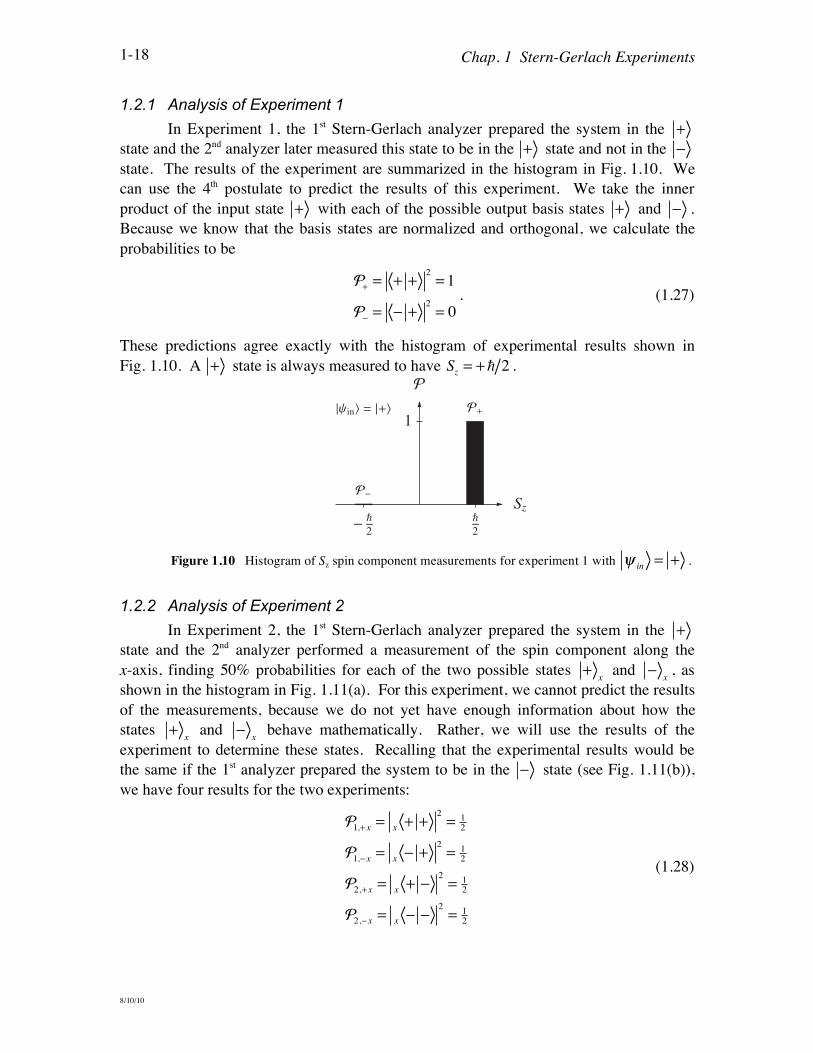
1.2.1 Analysis of Experiment 1

In Experiment 1, the 1st Stern-Gerlach analyzer prepared the system in the +

state and the 2nd analyzer later measured this state to be in the + state and not in the !

state. The results of the experiment are summarized in the histogram in Fig. 1.10. We

can use the 4th postulate to predict the results of this experiment. We take the inner

product of the input state + with each of the possible output basis states + and ! .

Because we know that the basis states are normalized and orthogonal, we calculate the

probabilities to be

!+= + +

2

= 1

!!= ! +

2

= 0

. (1.27)

These predictions agree exactly with the histogram of experimental results shown in

Fig. 1.10. A + state is always measured to have Sz= +! 2 .

- —2

—2

Sz

1

!

!-

!+†yin\ = †+\

Figure 1.10 Histogram of Sz spin component measurements for experiment 1 with !in

= + .

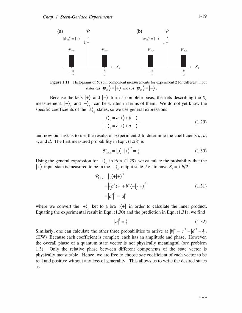
1.2.2 Analysis of Experiment 2

In Experiment 2, the 1st Stern-Gerlach analyzer prepared the system in the +

state and the 2nd analyzer performed a measurement of the spin component along the

x-axis, finding 50% probabilities for each of the two possible states +x and !

x, as

shown in the histogram in Fig. 1.11(a). For this experiment, we cannot predict the results

of the measurements, because we do not yet have enough information about how the

states +x and !

x behave mathematically. Rather, we will use the results of the

experiment to determine these states. Recalling that the experimental results would be

the same if the 1st analyzer prepared the system to be in the ! state (see Fig. 1.11(b)),

we have four results for the two experiments:

!1,+ x

=x+ +

2

=1

2

!1,! x

=x! +

2

=1

2

!2,+ x

=x+ !

2

=1

2

!2,! x

=x! !

2

=1

2

(1.28)


8/10/10

1-19

- —2

—2

Sx

1

!

!-x !+x

†yin\ = †+\

- —2

—2

Sx

1

!

!-x !+x

†yin\ = †-\(a) (b)

Figure 1.11 Histograms of Sx spin component measurements for experiment 2 for different input

states (a) !in

= + and (b) !in

= " .

Because the kets + and ! form a complete basis, the kets describing the Sx

measurement, +x and !

x, can be written in terms of them. We do not yet know the

specific coefficients of the ±x states, so we use general expressions

+

x= a + + b !

!x= c + + d !

, (1.29)

and now our task is to use the results of Experiment 2 to determine the coefficients a, b,

c, and d. The first measured probability in Eqn. (1.28) is

!1,+ x

=x+ +

2

=1

2 (1.30)

Using the general expression for +x in Eqn. (1.29), we calculate the probability that the

+ input state is measured to be in the +x output state, i.e., to have

Sx= +! 2 :

!1,+ x

=x+ +

2

= a*+ + b

*!{ } +

2

= a*2

= a2

(1.31)

where we convert the +x ket to a bra

x+ in order to calculate the inner product.

Equating the experimental result in Eqn. (1.30) and the prediction in Eqn. (1.31), we find

a2

=1

2 (1.32)

Similarly, one can calculate the other three probabilities to arrive at b2

= c2

= d2

=1

2.

(HW) Because each coefficient is complex, each has an amplitude and phase. However,

the overall phase of a quantum state vector is not physically meaningful (see problem

1.3). Only the relative phase between different components of the state vector is

physically measurable. Hence, we are free to choose one coefficient of each vector to be

real and positive without any loss of generality. This allows us to write the desired states

as


8/10/10

1-20

+

x=

1

2+ + e

i! "#$ %&

"x=

1

2+ + e

i' "#$ %&, (1.33)

where ! and ! are relative phases that we have yet to determine. Note that these states

are already normalized because we used all of the experimental results, which reflect the

fact that the probability for all possible results of an experiment must sum to unity.

We have used all the experimental results from Experiment 2, but the ±x kets

are still not determined. We need some more information. If we perform Experiment 1

with both analyzers aligned along the x-axis, the results will be as you expect—all +x

states from the 1st analyzer will be measured to have Sx= +! 2 at the 2nd analyzer, i.e.,

all atoms exit in the +x state and none in the !

x. The probability calculations for this

experiment are

!+ x=

x+ +

x

2

= 1

!! x=

x! +

x

2

= 0

, (1.34)

which tell us mathematically that the ±x states are orthonormal to each other, just like

the ± states. This also implies that the ±x kets form a basis, the Sx basis, which you

might expect because they correspond to the distinct results of a different spin component

measurement. The general expressions we used for the ±x kets are already normalized,

but are not yet orthogonal. That is the new piece of information we need. The

orthogonality condition leads to

x! +

x= 0

1

2+ + e

! i" !#$ %&1

2+ + e

i' !#$ %& = 0

1

21+ e

i '!"( )#$ %& = 0

ei '!"( )

= !1

ei'= !ei"

. (1.35)

where the complex conjugation of the second coefficient of the x! bra should be noted.

We now have an equation relating the remaining coefficients ! and ", but need

some more information to determine their values. Unfortunately, there is no more

information to be obtained, so we are free to choose the value of the phase !. This

freedom comes from the fact that we have required only that the x-axis be perpendicular

to the z-axis, which limits the x-axis only to a plane rather than to a unique direction. We

follow convention here and choose the phase ! = 0. Thus we can express the Sx basis

kets in terms of the Sz basis kets as

+

x=

1

2+ + !"# $%

!x=

1

2+ ! !"# $%

. (1.36)


8/10/10

1-21

We generally use the Sz basis as the preferred basis for writing general states, but

we could use any basis we choose. If we were to use the Sx basis, then we could write the

± kets as general states in terms of the ±x kets. This can be done by solving

Eqs. (1.36) for the ± kets, yielding

+ =

1

2+

x+ !

x"# $%

! =1

2+

x! !

x"# $%

. (1.37)

With respect to the measurements performed in Experiment 2, Eqn. (1.37) tells us

that the + state is a combination of the states +x and !

x. The coefficients tell us

that there is a 50% probability for measuring the spin component to be up along the

x-axis, and likewise for the down possibility, which is in agreement with the histogram of

measurements shown in Fig. 1.11(a). We must now take a moment to describe carefully

what a combinations of states, such as in Eqns. (1.36) and (1.37), is and what it is not.

1.2.3 Superposition states

A general spin-1/2 state vector ! can be expressed as a combination of the

basis kets + and !

! = a + + b " . (1.38)

We refer to such a combination of states as a superposition state. To understand the

importance of a quantum mechanical superposition state, consider the particular state

! = 1

2+ !+! "( ) . (1.39)

and measurements on this state, as shown in Fig. 1.12(a). Note that the state ! is none

other than the state +x that we found in Eqn. (1.36), so we already know what the

measurement results are. If we measure the spin component along the x-axis for this

state, then we record the result Sx= +! 2 with 100% probability (Experiment 1 with

both analyzers along the x-axis). If we measure the spin component along the orthogonal

z-axis, then we record the two results Sz= ±! 2 with 50% probability each

(Experiment 2 with the 1st and 2nd analyzers along the x– and z-axes, respectively). Based

upon this second set of results, one might be tempted to consider the state ! as

describing a beam that contains a mixture of atoms with 50% of the atoms in the +

state and 50% in the ! state. Such a state is called a mixed state, and is very different

from a superposition state.

To clarify the difference between a mixed state and a superposition state, let's

carefully examine the results of experiments on the proposed mixed state beam, as shown

in Fig. 1.12(b). If we measure the spin component along the z-axis, then each atom in the

+ state yields the result Sz= +! 2 with 100% certainty and each atom in the ! state

yields the result Sz= !! 2 with 100% certainty. The net result is that 50% of the atoms

yield Sz= +! 2 and 50% yield S

z= !! 2 . This is exactly the same result as that

obtained with all atoms in the +x state, as seen in Fig. 1.12(a). If we instead measure

the spin component along the x-axis, then each atom in the + state yields the two


8/10/10

1-22

results Sx= ±! 2 with 50% probability each (Experiment 2 with the 1st and 2nd analyzers

along the z- and x-axes, respectively). The atoms in the ! state yield the same results.

The net result is that 50% of the atoms yield Sx= +! 2 and 50% yield

Sx= !! 2 . This

is in stark contrast to the results of Experiment 1, which tells us that once we have

prepared the state to be +x, then subsequent measurements yield

Sx= +! 2 with

certainty, as seen in Fig. 1.12(a).

Z50

50

|y!=|+!x=[|+! + |"!]/$2

X100

0

Z50

50

50%50% |"!

X50

50

50%50% |"!

|y!=|+!x=[|+! + |"!]/$2

|+!

|+!

b)

a)

Figure 1.12 (a) Superposition state measurements and (b) mixed state measurements.

Hence we must conclude that the system described by the ! = +x state is not a

mixed state with some atoms in the + state and some in the ! state. Rather, each

atom in the +x beam is in a state that itself is a superposition of the + and ! states.

A superposition state is often called a coherent superposition because the relative phase

of the two terms is important. For example, if the input beam were in the !x state, then


8/10/10

1-23

there would be a relative minus sign between the two coefficients, which would result in

an Sx= !! 2 measurement but would not affect the Sz measurement.

We will not have any further need to speak of mixed states, so any combination of

states we use is a superposition state. Note that we cannot even write down a ket

describing a mixed state. So, if someone gives you a quantum state written as a ket, then

it must be a superposition state and not a mixed state. The random option in the SPINS

program produces a mixed state, while the unknown states are all superposition states.

Example 1.2

Consider the input state

!in

= 3 + + 4 " . (1.40)

Normalize this state vector and find the probabilities of measuring the spin component

along the z-axis to be Sz= ±! 2 .

To normalize this state, introduce an overall complex multiplicative factor and

solve for this factor by imposing the normalization condition:

!in

= C 3 + + 4 "#$ %&

!in!

in= 1

C*3 + + 4 "#$ %&{ } C 3 + + 4 "#$ %&{ } = 1

C*C 9 + + +12 + " +12 " + +16 " "#$ %& = 1

C*C 25[ ] = 1

C2

=1

25

, (1.41)

Because an overall phase is physically meaningless, we choose C to be real and positive:

C = 1 5 . Hence the normalized input state is

!in

=3

5+ +

4

5" . (1.42)

The probability of measuring Sz= +! 2 is

!+= + !

in

2

= +3

5+ +

4

5"#$ %&

2

=3

5+ + +

4

5+ "

2

=3

5

2

=9

25

(1.43)

The probability of measuring Sz= !! 2 is


8/10/10

1-24

!! = ! "in

2

= ! 3

5+ +

4

5!#$ %&

2

=3

5! + +

4

5! !

2

=4

5

2

=16

25

(1.44)

Note that the two probabilities add to unity, which indicates that we normalized the input

state properly. A histogram of the predicted measurement results is shown in Fig. 1.13.

- —2

—2

Sz

1

!

!-

!+

†yin\ = †+\ + †-\35

45

Figure 1.13 Histogram of Sz spin component measurements.

1.3 Matrix notation

Up to this point, we have defined kets mathematically in terms of their inner

products with other kets. Thus in the general case we write a ket as

! = + ! ! + !!+!! " ! ! " , (1.45)

or in a specific case, we write

+

x= + +

x! + !!+!! ! +

x! !

=1

2+ +

1

2!

. (1.46)

In both of these cases, we have chosen to write the kets in terms of the + and ! basis

kets. If we agree on that choice of basis as a convention, then the two coefficients + +x

and ! +x uniquely specify the quantum state, and we can simplify the notation by using

those just numbers. Thus, we represent a ket as a column vector containing the two

coefficients that multiply each basis ket. For example, we represent +x as

+x!

1

2

1

2

!

"##

$

%&&

, (1.47)

where we have used the new symbol ! to signify "is represented by", and it is

understood that we are using the + and ! basis or the Sz basis. We cannot say that

the ket equals the column vector, because the ket is an abstract vector in the state space


8/10/10

1-25

and the column vector is just two complex numbers. If we were to choose a different

basis for representing the vector, then the complex coefficients would be different even

though the vector is unchanged. We need to have a convention for the ordering of the

amplitudes in the column vector. The standard convention is to put the spin up amplitude

first (at the top). Thus the representation of the !x state (Eqn. (1.37)) is

!x!

1

2

! 1

2

"

#$$

%

&''

(!! +

(!! !. (1.48)

where we have explicitly labeled the rows according to their corresponding basis kets.

Using this convention, it should be clear that the basis kets themselves are written as

+ !1

0

!

"#$

%&

' ! 0

1

!

"#$

%&

. (1.49)

This demonstrates the important feature that basis kets are unit vectors when written in

their own basis.

This new way of expressing a ket simply as the collection of coefficients that

multiply the basis kets is referred to as a representation. Because we have assumed the

Sz kets as the basis kets, this is called the Sz representation. It is always true that basis

kets have the simple form shown in Eq. (1.49) when written in their own representation.

A general ket ! is written as

! !

+ !

" !

#

$%%

&

'((

. (1.50)

This use of matrix notation simplifies the mathematics of bras and kets. The advantage is

not so evident for the simple 2-dimensional state space of spin-1/2 systems, but it is very

evident for larger dimensional problems. This notation is indispensable when using

computers to calculate quantum mechanical results. For example, the SPINS program

employs matrix calculations coded in the Java computer language to simulate the Stern-

Gerlach experiments using the same probability rules you are learning here.

We saw earlier (Eqn. (1.11)) that the coefficients of a bra are the complex

conjugates of the coefficients of the corresponding ket. We also know that an inner

product of a bra and a ket yields a single complex number. In order for the matrix rules

of multiplication to be used, a bra must be represented by a row vector, with the entries

being the coefficients ordered in the same sense as for the ket. For example, if we use the

general ket

! = a + + b " , (1.51)

which is represented as


8/10/10

1-26

! !a

b

"

#$%

&', (1.52)

then the corresponding bra

! = a*+ + b

*" (1.53)

is represented by a row vector as

! ! a

*b*( ) . (1.54)

The rules of matrix algebra can then be applied to find an inner product. For example,

! ! = a

*b*( ) a

b

"

#$%

&'

= a2

+ b2

. (1.55)

So a bra is represented by a row vector that is the complex conjugate and transpose of the

column vector representing the corresponding ket.

Example 1.3:

To get some practice using this new matrix notation, and to learn some more

about the spin-1/2 system, use the results of Experiment 2 to determine the Sy basis kets

using the matrix approach instead of the Dirac bra-ket approach.

Consider Experiment 2 in the case where the 2nd Stern-Gerlach analyzer is aligned

along the y-axis. We said before that the results are the same as in the case shown in

Fig. 1.4. Thus we have

!1,+ y

=y+ +

2

=1

2

!1,! y

=y! +

2

=1

2

!2,+ y

=y+ !

2

=1

2

!2,! y

=y! !

2

=1

2

. (1.56)

as depicted in the histograms of Fig. 1.14.

These results allows us to determine the kets ±y corresponding to the spin

component up and down along the y-axis. The argument and calculation proceeds

exactly as it did earlier for the ±x states up until the point (Eqn. (1.35)) where we

arbitrarily choose the phase ! to be zero. Having done that for the ±x states, we are no

longer free to make that same choice for the ±y states. Thus we use Eqn. (1.35) to

write the ±y states as


8/10/10

1-27

- —2

—2

Sy

1

!

!-y !+y

†yin\ = †+\

- —2

—2

Sy

1

!

!-y !+y

†yin\ = †-\(a) (b)

Figure 1.14 Histograms of Sy spin component measurements for input states (a) !in

= +

and (b) !in

= " .

+y=

1

2+ + e

i! "#$ %& !1

2

1

ei!

'

()*

+,

"y=

1

2+ " ei! "#$ %& !

1

2

1

"ei!'

()*

+,

(1.57)

To determine the phase !, we use some more information at our disposal. Experiment 2

could be performed with the 1st Stern-Gerlach analyzer aligned along the x-axis and the

2nd analyzer along the y-axis. Again the results would be identical (50% at each output

port), yielding

!+ y=

y+ +

x

2

=1

2 (1.58)

as one of the measured quantities. Now use matrix algebra to calculate this:

y+ +

x= 1

21 e

! i"( ) 1

2

1

1

#

$%&

'(

= 1

21+ e

! i"( )

y+ +

x

2

= 1

21+ e

! i"( ) 1

21+ e

i"( )

= 1

41+ e

i"+ e

! i"+1( )

= 1

21+ cos"( ) = 1

2

(1.59)

This result requires that cos! = 0, or that ! = ±" 2 . The two choices for the phase

correspond to the two possibilities for the direction of the y-axis relative to the already

determined x- and z-axes. The choice ! = +" 2 can be shown to correspond to a

right-handed coordinate system, which is the standard convention, so we choose that

phase. We thus represent the ±y kets as


8/10/10

1-28

+y!

1

2

1

i

!

"#$

%&

'y!

1

2

1

'i!

"#$

%&

(1.60)

Note that the imaginary components of these kets are required. They are not merely a

mathematical convenience as one sees in classical mechanics. In general, quantum

mechanical state vectors have complex coefficients. But this does not mean that the

results of physical measurements are complex. On the contrary, we always calculate a

measurement probability using a complex square, so all quantum mechanics predictions

of probabilities are real.

1.4 General Quantum Systems

The machinery we have developed for spin-1/2 systems can be generalized to

other quantum systems. For example, if an observable A yields quantized measurement

results an for some finite range of n, then we generalize the schematic depiction of a

Stern-Gerlach measurement to a measurement of the observable A, as shown in Fig. 1.15.

The observable A labels the measurement device and the possible results a1, a2, a3, etc.

label the output ports. The basis kets corresponding to the results an are then an

. The

mathematical rules about kets in this general case are

aiaj= !

ij !!!!!!orthonormality

" = ai" ! a

i

i

# completeness (1.61)

where we use the Kronecker delta

!ij=

0

1

i " j

i = j

#$%

&% (1.62)

to express the orthonormality condition compactly. In this case, the generalization of

postulate 4 says that the probability of a measurement of one of the possible results an is

!an

= an!

in

2

(1.63)

A|a1!

|a2!

|a3!

|%in! a2a1

a3

Figure 1.15 Generic depiction of the quantum mechanical measurement of observable A.


8/10/10

1-29

Example 1.4.

Imagine a quantum system with an observable A that has three possible

measurement results: a1, a2, and a3. The three kets a1

, a2

, and a3

corresponding to

these possible results form a complete orthonormal basis. The system is prepared in the

state

! = 2 a1" 3 a

2+ 4i a

3 (1.64)

Calculate the probabilities of all possible measurement results of the observable A.

The state vector in Eqn. (1.64) is not normalized, so we must normalize it before

calculating probabilities. Introducing a complex normalization constant C, we find

1= ! !

= C*2 a

1" 3 a

2" 4i a

3( )C 2 a1" 3 a

2+ 4i a

3( )

= C2

4 a1a1" 6 a

1a2+ 8i a

1a3{

!!!!!!!!!!!"6 a2a1+ 9 a

2a2"12i a

2a3

!!!!!!!!!!!"8i a3a1+12i a

3a2+16 a

3a3 }

= C2

4 + 9 +16{ } = C2

29

#C =1

29

(1.65)

The normalized state is

! =1

292 a

1" 3 a

2+ 4i a

3( ) (1.66)

The probabilities of measuring the results a1, a2, and a3 are

!a1= a

1!

2

= a1

1

292 a

1" 3 a

2+ 4i a

3{ }2

=1

292 a

1a1" 3 a

1a2+ 4i a

1a3

2

=4

29

!a2= a

2!

2

= a2

1

292 a

1" 3 a

2+ 4i a

3{ }2

=9

29

!a3= a

3!

2

= a3

1

292 a

1" 3 a

2+ 4i a

3{ }2

=16

29

(1.67)

A schematic of this experiment is shown in Fig. 1.16(a) and a histogram of the predicted

probabilities is shown in Fig. 1.16(b).


8/10/10

1-30

A|%in! a2a1

a3

a) b)

929!a2 =

429!a1 =

1629!a3 = a1 a2 a3

A

1!

!a1!a2

!a3

Figure 1.16 (a) Schematic diagram of the measurement of observable A and (b) histogram of

the predicted measurement probabilities.

1.5 Postulates

We have introduced two of the postulates of quantum mechanics in this chapter.

The postulates of quantum mechanics dictate how to treat a quantum mechanical system

mathematically and how to interpret the mathematics to learn about the physical system

in question. These postulates cannot be proven, but they have been successfully tested by

many experiments, and so we accept them as an accurate way to describe quantum

mechanical systems. New results could force us to reevaluate these postulates at some

later time. All six postulates are listed below to give you an idea where we are headed

and a framework into which you can place the new concepts as we confront them.

Postulates of Quantum Mechanics

1. The state of a quantum mechanical system, including all the information

you can know about it, is represented mathematically by a normalized ket

! .

2. A physical observable is represented mathematically by an operator A that

acts on kets.

3. The only possible result of a measurement of an observable is one of the

eigenvalues an of the corresponding operator A.

4. The probability of obtaining the eigenvalue an in a measurement of the

observable A on the system in the state ! is

!an

= an!

2

,

where an

is the normalized eigenvector of A corresponding to the

eigenvalue an.

5. After a measurement of A that yields the result an, the quantum system is

in a new state that is the normalized projection of the original system ket

onto the ket (or kets) corresponding to the result of the measurement:

!" =Pn"

" Pn"

.


8/10/10

1-31

6. The time evolution of a quantum system is determined by the Hamiltonian

or total energy operator H(t) through the Schrödinger equation

i!d

dt! t( ) = H t( ) ! t( ) .

As you read these postulates for the first time, you will undoubtedly encounter

new terms and concepts. Rather than explain them all here, the plan of this text is to

continue to explain them through their manifestation in the Stern-Gerlach spin-1/2

experiment. We have chosen this example because it is inherently quantum mechanical

and forces us to break away from reliance on classical intuition or concepts. Moreover,

this simple example is a paradigm for many other quantum mechanical systems. By

studying it in detail, we can appreciate much of the richness of quantum mechanics.

1.6 Summary

Through the Stern-Gerlach experiment we have learned several key concepts

about quantum mechanics in this chapter.

• Quantum mechanics is probabilistic.

We cannot predict the results of experiments precisely. We can predict

only the probability that a certain result is obtained in a measurement.

• Spin measurements are quantized.

The possible results of a spin component measurement are quantized.

Only these discrete values are measured.

• Quantum measurements disturb the system.

Measuring one physical observable can "destroy" information about other

observables.

We have learned how to describe the state of a quantum mechanical system

mathematically using a ket, which represents all the information we can know about that

state. The kets + and ! result when the spin component Sz along the z-axis is

measured to be up or down, respectively. These kets form an orthonormal basis, which

we denote by the inner products

+ + = 1

! ! = 1

+ ! = 0

(1.68)

The basis is also complete, which means that it can be used to express all possible kets as

superposition states

! = a + + b " . (1.69)

For spin component measurements, the kets corresponding to spin up or down

along the three Cartesian axes are


8/10/10

1-32

+ !!!!!!! +x=1

2+ + !"# $%!!!!!!! +

y=1

2+ + i !"# $%

! !!!!!!! !x=1

2+ ! !"# $%!!!!!!! !

y=1

2+ ! i !"# $%

(1.70)

We also found it useful to introduce a matrix notation for calculations. In this matrix

language the kets in Eqn. (1.70) are represented by

+ ! 1

0

!

"#$

%&!!!!!!! +

x!

1 2

1 2

!

"##

$

%&&!!!!!!!!!! +

y!

1 2

i 2

!

"##

$

%&&!!

' ! 0

1

!

"#$

%&!!!!!!! '

x!

1 2

'1 2

!

"##

$

%&&!!!!!!! '

y!

1 2

'i 2

!

"##

$

%&&

(1.71)

The most important tool we have learned so far is the probability postulate

(postulate 4). To calculate the probability that a measurement on an input state !in

will

yield a particular result, for example Sz= ! 2 , we complex square the inner product of

the input state with the ket corresponding to the measured result, + in this case:

!+= + !

in

2

(1.72)

This is generalized to other systems where a measurement yields a particular result an

corresponding to the ket an

as:

!an

= an!

in

2

(1.73)

1.7 Problems

1.1 Consider the following state vectors:

!1= 3 + + 4 "

!2= + + 2i "

!3= 3 + " e

i# 3"

a) Normalize each state vector.

b) For each state vector, calculate the probability that the spin component is up

or down along each of the three Cartesian axes. Use bra-ket notation for the

entire calculation.

c) Write each normalized state in matrix notation.

d) Repeat part (b) using matrix notation for the entire calculation.


8/10/10

1-33

1.2 Consider the three quantum states:

!1=1

3+ + i

2

3"

!2=1

5+ "

2

5"

!3=1

2+ +

ei# 4

2"

Use bra-ket notation (not matrix notation) to solve the following problems. Note

that + + = 1 , ! ! = 1 , and + ! = 0 .

a) For each of the !i

above, find the normalized vector !i

that is orthogonal

to it.

b) Calculate the inner products ! i!

j for i and j = 1, 2, 3.

1.3 Show that a change in the overall phase of a quantum state vector does not change the probability of obtaining a particular result in a measurement. To do this,

consider how the probability is affected by changing the state ! to the state

ei! " .

1.4 Show by explicit bra-ket calculations using the states in Eqn. (1.29) that the four

experimental results in Eqn. (1.28) lead to the results b2

= c2

= d2

=1

2.

1.5 A beam of spin-! particles is prepared in the state

! =2

13+ + i

3

13"

a) What are the possible results of a measurement of the spin component Sz, and

with what probabilities would they occur?

b) What are the possible results of a measurement of the spin component Sx, and


c) Plot histograms of the predicted measurement results from parts (a) and (b).

1.6 A beam of spin-! particles is prepared in the state

! =2

13+

x+ i

3

13"

x




8/10/10

1-34

b) What are the possible results of a measurement of the spin component Sx, and


c) Plot histograms of the predicted measurement results from parts (a) and (b).

1.7 A classical coin is thrown in the air and lands on the ground, where a

measurement is made of its state.

a) What are the possible results of this measurement?

b) What are the predicted probabilities for these possible outcomes?

c) Plot a histogram of the predicted measurement results.

1.8 A classical cubical die is thrown onto a table and comes to rest, where a

measurement is made of its state.




1.9 A pair of dice (classical cubes) are thrown onto a table and come to rest, where a

measurement is made of the state of the system (i.e., the sum of the two die).




1.10 Consider the three quantum states:

!1=4

5+ + i

3

5"

!2=4

5+ " i

3

5"

!3= "

4

5+ + i

3

5"

a) For each of the !i

above, calculate the probabilities of spin component

measurements along the x-, y-, and z-axes.

b) Use your results from (a) to comment on the importance of the overall phase

and of the relative phases of the quantum state vector.

1.11 A spin-! particle is prepared in the state

! =3

34+ + i

5

34"


8/10/10

1-35



b) Suppose that the Sz measurement on the particle yields the result Sz= !! 2 .

Subsequent to that result a second measurement is performed to measure the

spin component Sx. What are the possible results of that measurement, and


c) Draw a schematic diagram depicting the successive measurements in parts (a)

and (b).

1.12 Consider a quantum system with an observable A that has three possible

measurement results: a1, a2, and a3. Write down the orthogonality, normalization,

and completeness relations for the three kets comprising the basis corresponding

to the possible results of the A measurement.

1.13 Consider a quantum system with an observable A that has three possible

measurement results: a1, a2, and a3.

a) Write down the three kets a1

, a2

, and a3

corresponding to these possible

results using matrix notation.

b) The system is prepared in the state

! = 1 a1" 2 a

2+ 5 a

3

Write this state in matrix notation and calculate the probabilities of all

possible measurement results of the observable A. Plot a histogram of the

predicted measurement results.

c) In a different experiment, the system is prepared in the state

! = 2 a1+ 3i a

2

Write this state in matrix notation and calculate the probabilities of all

possible measurement results of the observable A. Plot a histogram of the

predicted measurement results.

1.14 Consider a quantum system in which the energy E is measured and there are four

possible measurement results: 2 eV, 4 eV, 7 eV, and 9 eV.

a) The system is prepared in the state

! =1

393 2!eV " i 4 !eV + 2e

i# 77!eV + 5 9!eV{ }

Calculate the probabilities of all possible measurement results of the energy E.

Plot a histogram of the predicted measurement results.


8/10/10

1-36

1.15 Consider a quantum system described by a basis a1

, a2

, and a3

. The system

is initially in a state

!i=

i

3a1+

2

3a2

.

Find the probability that the system is measured to be in the final state

! f =1+ i

3a1+1

6a2+1

6a3

.

1.16 The spin components of a beam of atoms prepared in the state !in

are measured

and the following experimental probabilities are obtained:

!+=

1

2!+ x=

3

4!+ y= 0.067

!!=

1

2!! x=

1

4!! y= 0.933

From the experimental data, determine the input state.

1.17 In part (1) of SPINS Lab #2, you measured the probabilities of all the possible

spin components for each of the unknown initial states !i

(i = 1, 2, 3, 4). Using

your data from that lab, find the unknown states !1

, !2

, !3

and !4

.

Express each of the unknown states as a linear superposition of the Sz basis states

+ and ! . For each state, use your result to calculate the theoretical values of

the probabilities for each component measurement and compare these theoretical

predictions with your experimental results.

1.8 Resources

1.8.1 Activities

SPINS: A software program to simulate Stern-Gerlach spin experiments. The Java

software runs on all platforms and can be downloaded in two forms:

Open Source Physics framework

www.physics.oregonstate.edu/~mcintyre/ph425/spins/index_SPINS_OSP.html

or

Standalone Java

www.physics.oregonstate.edu/~mcintyre/ph425/spins


8/10/10

1-37

SPINS Lab 1: An introduction to successive Stern-Gerlach spin 1/2 measurements. The

randomness of measurements is demonstrated and students use statistical analysis

to deduce probabilities from measurements.

www.physics.oregonstate.edu/portfolioswiki/doku.php?id=activities:main&file=s

pin1

SPINS Lab 2: Students deduce unknown quantum state vectors from measurements of

spin projections. (part 3 requires material from Chap. 2 to do the calculations)

www.physics.oregonstate.edu/portfolioswiki/doku.php?id=activities:main&file=s

pin2

A different simulation of the Stern-Gerlach experiment (somewhat Flashier):

phet.colorado.edu/simulations/sims.php?sim=SternGerlach_Experiment

1.8.2 Further reading

The history of the Stern-Gerlach experiment and how a bad cigar helped are chronicled in

a Physics Today article:

B. Friedrich and D. Herschbach, "Stern and Gerlach: How a Bad Cigar Helped

Reorient Atomic Physics," Phys. Today 56, 53-59 (2003).

http://dx.doi.org/10.1063/1.1650229

Nature has published a supplement on the milestones in spin physics. An extensive

timeline of historical events, review articles, and links to original articles are

included.

Nature Phys. 4, S1-S43 (2008). www.nature.com/milestones/spin

The SPINS lab software is described in this pedagogical article:

D. V. Schroeder and T. A. Moore, "A computer-simulated Stern-Gerlach

laboratory," Am. J. Phys. 61, 798-805 (1993).

Some other textbooks that take a spins-first approach or have an extensive treatment of

Stern-Gerlach experiments:

R. P. Feynman, R. B. Leighton, and M. Sands, The Feynman Lectures on Physics,

Volume 3, Quantum Mechanics, Addison-Wesley Publishing Company, Inc.,

Reading, Massachusetts, 1965.

J. J. Sakurai, Modern Quantum Mechanics, Addison-Wesley Publishing

Company, Inc., Redwood City, California, 1985.

J. S. Townsend, A Modern Approach to Quantum Mechanics, McGraw Hill, Inc.,

New York, 1992.


8/10/10

1-38

C. Cohen-Tannoudji, B. Diu, and F. Laloë, Quantum Mechanics, John Wiley &

Sons, New York, 1977.

Chapter 1 STERN-GERLACH EXPERIMENTSdepts.washington.edu/jrphys/ph248A11/qmch1.pdf · Chap. 1...

Documents

Transcript of Chapter 1 STERN-GERLACH EXPERIMENTSdepts.washington.edu/jrphys/ph248A11/qmch1.pdf · Chap. 1...