CE 416.3 Class Notes I.R. Fleming Page 1

Chapter 1 - Soil Mechanics Review Part A

1.1 Introduction

Geotechnical Engineer is concerned with predicting / controlling

Failure/Stability Deformations Influence of water (Seepage etc.)

• Soil behavour is complex: - Anisotropic - Non-homogeneous - Non-linear - Stress and stress history dependant

• Complexity gives rise to importance of: - Theory - Lab tests - Field tests - Empirical relations - Computer applications - Experience, Judgement, FOS

Unlike steel, soil properties can’t be easily determined with a single grade#: - the best we can do:

Soil Texture Phase relationships Atterberg Limits Clay mineralogy Fabric and structure Genetic Factors Classification

1.2 Soil Texture

• Particle size, shape and size distribution - Coarse-textured (Gravel, Sand) - Fine-textured (Silt, Clay) - visibility by the naked eye (0.05mm is the approx limit)

CE 416.3 Class Notes I.R. Fleming Page 2

There are several Classification systems with some differences: we use USCS: • Particle size distribution

- Sieve/Mechanical analysis or Gradation Test - Hydrometer analysis for smaller than .05 to .075 mm (#200 US

Standard sieve) • Particle size distribution curves

- Well graded - Poorly graded

Cu & Cc together provides a better indication of if a soil is well graded

Particle Shape: Roundness vs Angularity Sphericity

Higher angularity tends to give higher strength for gravels and sands. Modulus: Not certain

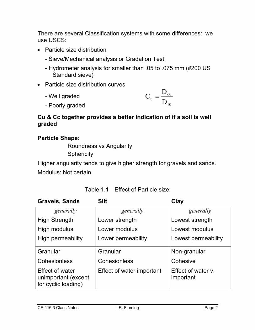
Table 1.1 Effect of Particle size:

Gravels, Sands Silt Clay generally

High Strength High modulus High permeability

generally Lower strength Lower modulus Lower permeability

generally Lowest strength Lowest modulus Lowest permeability

Granular Cohesionless Effect of water unimportant (except for cyclic loading)

Granular Cohesionless Effect of water important

Non-granular Cohesive Effect of water v. important

10

60u D

DC =

CE 416.3 Class Notes I.R. Fleming Page 3

Particle size distribution:

Important for gravels and sands - well graded material gives higher strength and higher modulus

For some sands D10 can be related to Permeability, but D10 relates poorly to K for silts and clays

Soil is Particulate in Nature

• Properties of interest – strength (stability) and compressibility (settlement)

• Phases – solid, liquid, vapour and others?

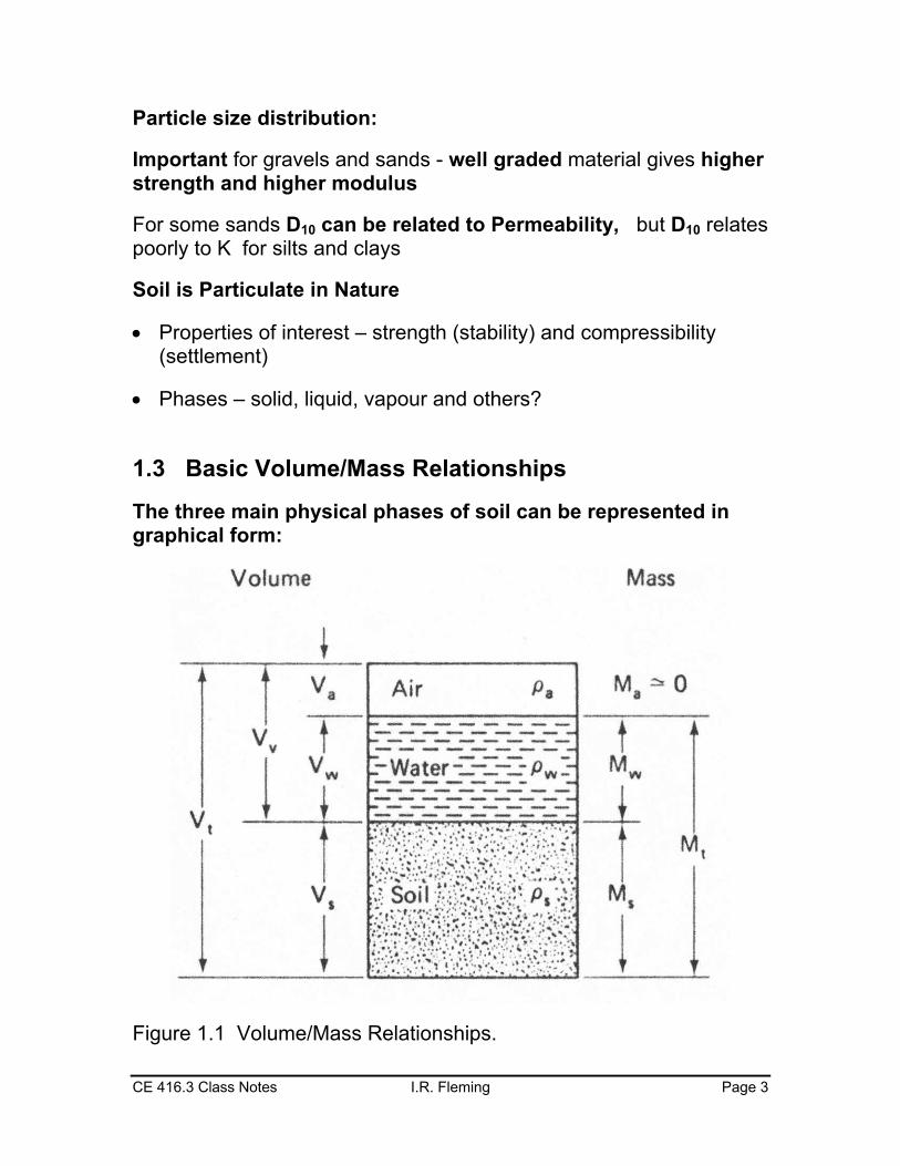
1.3 Basic Volume/Mass Relationships

The three main physical phases of soil can be represented in graphical form:

Figure 1.1 Volume/Mass Relationships.

CE 416.3 Class Notes I.R. Fleming Page 4

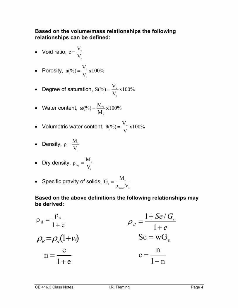
Based on the volume/mass relationships the following relationships can be defined:

• Void ratio, s

v

VVe =

• Porosity, x100%VVn(%)

t

v=

• Degree of saturation, x100%VVS(%)

v

w=

• Water content, x100%MMω(%)

s

w=

• Volumetric water content, x100%VVθ(%) w=

• Density, t

t

VMρ =

• Dry density, t

sdry V

Mρ =

• Specific gravity of solids, swater

ss Vρ

MG =

Based on the above definitions the following relationships may be derived:

e1s

d +ρ

=ρeGSe s

B ++

=1

/1ρ

)1( wdB +=ρρ swGSe =

e1en+

=n1

ne−

=

CE 416.3 Class Notes I.R. Fleming Page 5

When solving problems with phase relations:

if possible, choose one quantity to be UNITY and determine the remaining quantities similar to solving a crossword puzzle (i.e. filling the remaining blanks on the phase diagram)

Void Ratio:

Generally (for the same soil)

- modulus increases with decreasing void ratio - strength increases with decreasing void ratio - provides an indication of stress history

Moisture content:

Saturated moisture content is directly proportional to void ratio.

Given that Gs is typically between 2.6 to 2.8, all other phase relations depend on w and e.

Generally, water content or void ratio alone may not tell much about soil properties when comparing two soils.

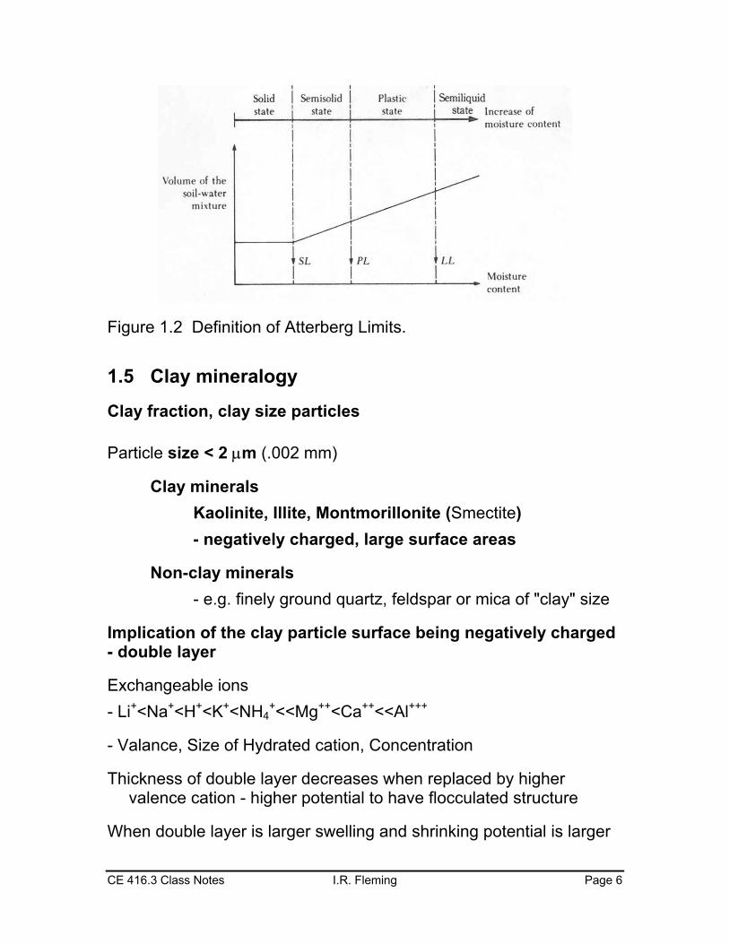
1.4 Atterberg Limits Atterberg limits are defined as limits of engineering behavior based on water contents

• Liquid limit (LL) – the water content, in percent, at which the soil changes from a liquid to a plastic state

• Plastic limit (PL) – the water content, in percent, at which the soil changes from a plastic to a semisolid state

• Shrinkage limit (SL) – the water content, in percent, at which the soil changes from a semisolid to a solid state

• Plasticity index (PI) – the difference between the liquid limit and plastic limit of a soil, PLLLPI −=

CE 416.3 Class Notes I.R. Fleming Page 6

Figure 1.2 Definition of Atterberg Limits.

1.5 Clay mineralogy

Clay fraction, clay size particles

Particle size < 2 µm (.002 mm)

Clay minerals Kaolinite, Illite, Montmorillonite (Smectite) - negatively charged, large surface areas

Non-clay minerals - e.g. finely ground quartz, feldspar or mica of "clay" size

Implication of the clay particle surface being negatively charged - double layer

Exchangeable ions - Li+<Na+<H+<K+<NH4

+<<Mg++<Ca++<<Al+++

- Valance, Size of Hydrated cation, Concentration

Thickness of double layer decreases when replaced by higher valence cation - higher potential to have flocculated structure

When double layer is larger swelling and shrinking potential is larger

CE 416.3 Class Notes I.R. Fleming Page 7

Soils containing clay minerals tend to be cohesive and plastic.

Given the existence of a double layer, clay minerals have an affinity for water and hence has a potential for swelling (e.g. during wet season) and shrinking (e.g. during dry season). Smectites such as Montmorillonite have the highest potential, Kaolinite has the lowest.

Generally, a flocculated soil has higher strength, lower compressibility and higher permeability compared to a non-flocculated soil.

Sands and gravels (cohesionless ) : Relative density can be used to compare the same soil. However, the fabric may be different for a given relative density and hence the behaviour.

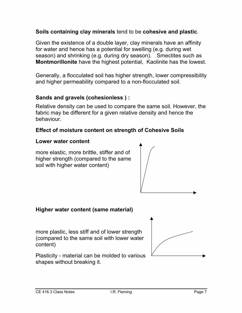
Effect of moisture content on strength of Cohesive Soils

Lower water content

more elastic, more brittle, stiffer and of higher strength (compared to the same soil with higher water content)

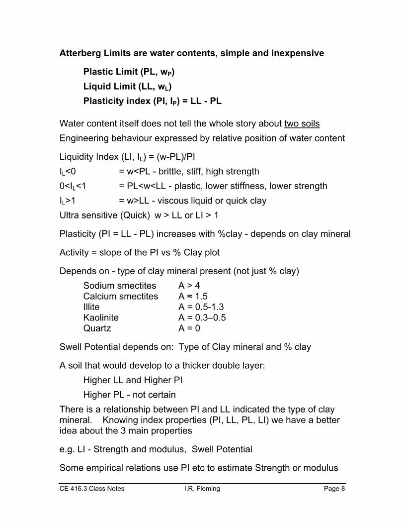
Higher water content (same material)

more plastic, less stiff and of lower strength (compared to the same soil with lower water content)

Plasticity - material can be molded to various shapes without breaking it.

CE 416.3 Class Notes I.R. Fleming Page 8

Atterberg Limits are water contents, simple and inexpensive

Plastic Limit (PL, wP) Liquid Limit (LL, wL) Plasticity index (PI, IP) = LL - PL

Water content itself does not tell the whole story about two soils Engineering behaviour expressed by relative position of water content

Liquidity Index (LI, IL) = (w-PL)/PI IL<0 = w<PL - brittle, stiff, high strength 0<IL<1 = PL<w<LL - plastic, lower stiffness, lower strength IL>1 = w>LL - viscous liquid or quick clay Ultra sensitive (Quick) w > LL or LI > 1

Plasticity (PI = LL - PL) increases with %clay - depends on clay mineral

Activity = slope of the PI vs % Clay plot

Depends on - type of clay mineral present (not just % clay) Sodium smectites A > 4 Calcium smectites A ≈ 1.5 Illite A = 0.5-1.3 Kaolinite A = 0.3–0.5 Quartz A = 0

Swell Potential depends on: Type of Clay mineral and % clay

A soil that would develop to a thicker double layer: Higher LL and Higher PI

Higher PL - not certain There is a relationship between PI and LL indicated the type of clay mineral. Knowing index properties (PI, LL, PL, LI) we have a better idea about the 3 main properties

e.g. LI - Strength and modulus, Swell Potential

Some empirical relations use PI etc to estimate Strength or modulus

CE 416.3 Class Notes I.R. Fleming Page 9

1.6 Soil Classification Systems • Classification may be based on – grain size, genesis, Atterberg

Limits, behavior, etc. In Engineering, descriptive or behaviour-based classification is more useful than genetic classification.

American Assoc of State Highway & Transportation Officials (AASHTO) • Originally proposed in 1945 • Classification system based on eight major groups (A-1 to A-8)

and a group index • Based on grain size distribution, liquid limit and plasticity indices • Mainly used for highway subgrades in USA

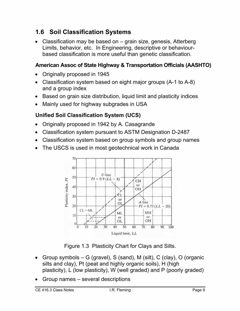
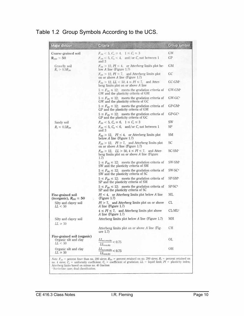
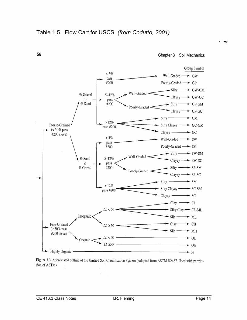
Unified Soil Classification System (UCS) • Originally proposed in 1942 by A. Casagrande • Classification system pursuant to ASTM Designation D-2487 • Classification system based on group symbols and group names • The USCS is used in most geotechnical work in Canada

Figure 1.3 Plasticity Chart for Clays and Silts.

• Group symbols – G (gravel), S (sand), M (silt), C (clay), O (organic silts and clay), Pt (peat and highly organic soils), H (high plasticity), L (low plasticity), W (well graded) and P (poorly graded)

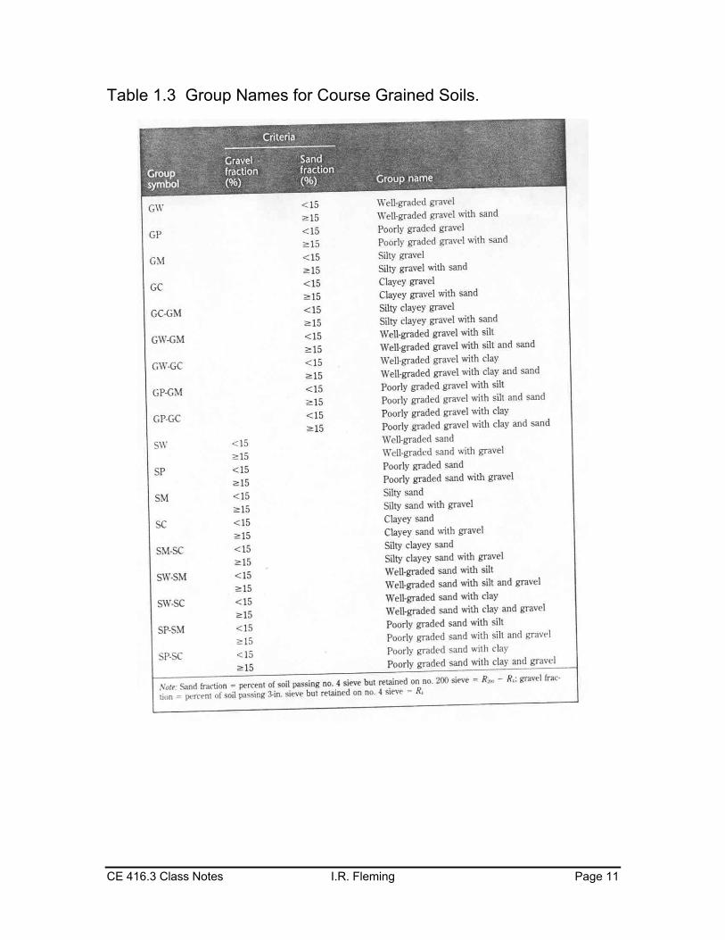
• Group names – several descriptions

CE 416.3 Class Notes I.R. Fleming Page 10

Table 1.2 Group Symbols According to the UCS.

CE 416.3 Class Notes I.R. Fleming Page 11

Table 1.3 Group Names for Course Grained Soils.

CE 416.3 Class Notes I.R. Fleming Page 12

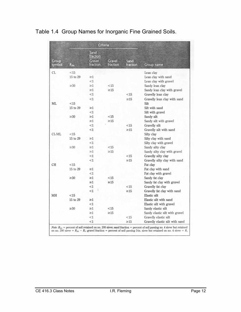
Table 1.4 Group Names for Inorganic Fine Grained Soils.

CE 416.3 Class Notes I.R. Fleming Page 13

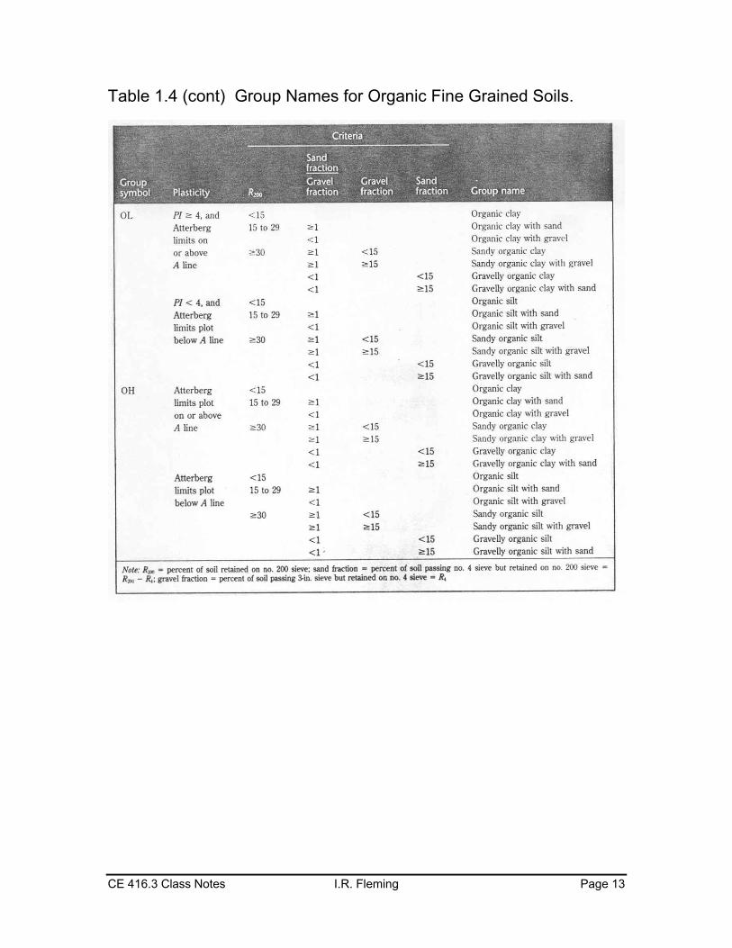
Table 1.4 (cont) Group Names for Organic Fine Grained Soils.

CE 416.3 Class Notes I.R. Fleming Page 14

Table 1.5 Flow Cart for USCS (from Codutto, 2001)

CE 416.3 Class Notes I.R. Fleming Page 15

1.7 Permeability & Seepage

• Flow through soils affect several material properties such as shear strength and compressibility

• If there were no water in soil, there would be no geotechnical engineering

Darcy’s Law

• Developed in 1856

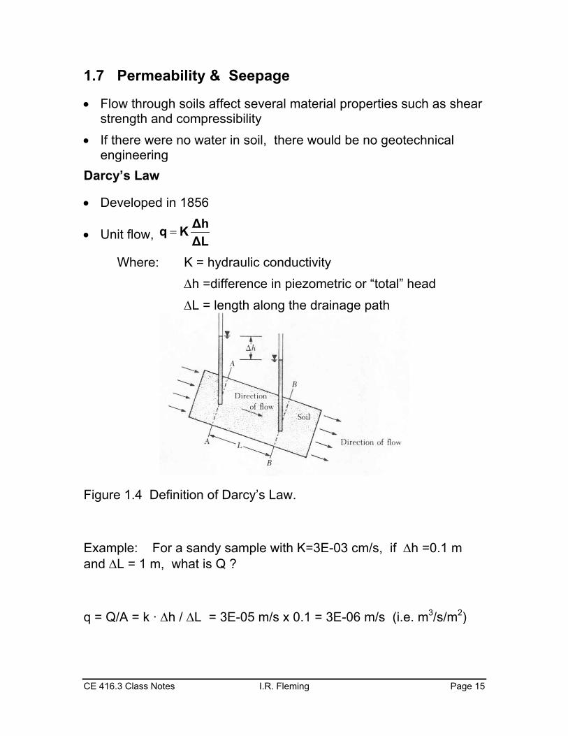
• Unit flow, ∆L∆hKq =

Where: K = hydraulic conductivity ∆h =difference in piezometric or “total” head ∆L = length along the drainage path

Figure 1.4 Definition of Darcy’s Law.

Example: For a sandy sample with K=3E-03 cm/s, if ∆h =0.1 m and ∆L = 1 m, what is Q ?

q = Q/A = k · ∆h / ∆L = 3E-05 m/s x 0.1 = 3E-06 m/s (i.e. m3/s/m2)

CE 416.3 Class Notes I.R. Fleming Page 16

1-D Seepage Q = k i A i = hydraulic gradient =∆h /∆L ∆h = change in TOTAL head Downward seepage increases effective stress Upward seepage decreases effective stress

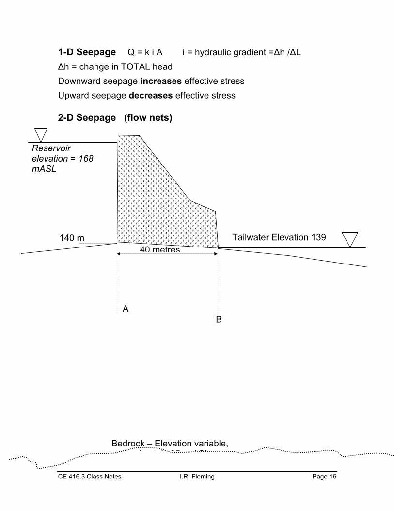
2-D Seepage (flow nets)

40 metres140 m

Bedrock – Elevation variable, i t l 95 ASL

A B

Tailwater Elevation 139 ASL

Reservoir elevation = 168 mASL

CE 416.3 Class Notes I.R. Fleming Page 17

1.7 Effective Stress

• Effective stress is defined as the effective pressure that occurs at a specific point within a soil profile

• The total stress is carried partially by the pore water and partially by the soil solids, the effective stress, σ’, is defined as the total stress, σt, minus the pore water pressure, u, uσσ' t −=

• Changes in effective stress is responsible for volume change

• The effective stress is responsible for producing frictional resistance between the soil solids

• Therefore, effective stress is an important concept in geotechnical engineering

• Overconsolidation ratio, z

'c

'

σσOCR =

Where: σ´c = preconsolidation pressure

• Critical hydraulic gradient σ′=0 when i = (γB-γw) /γw → σ’ = 0

CE 416.3 Class Notes I.R. Fleming Page 18

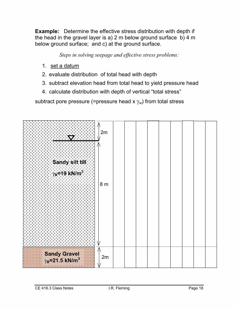
Example: Determine the effective stress distribution with depth if the head in the gravel layer is a) 2 m below ground surface b) 4 m below ground surface; and c) at the ground surface.

Steps in solving seepage and effective stress problems:

1. set a datum 2. evaluate distribution of total head with depth 3. subtract elevation head from total head to yield pressure head 4. calculate distribution with depth of vertical “total stress”

subtract pore pressure (=pressure head x γw) from total stress

Sandy silt till

γB=19 kN/m3

2m

Sandy Gravel γB=21.5 kN/m3

8 m

2m