
Chapter 1 LABOR AS A PRODUCTIVE FACTORcs.uef.fi/~estola/mikro2/chapter7.pdf · LABOR AS A...
26
Chapter 1 LABOR AS A PRODUCTIVE FACTOR Definition : By the derived demand of production factors we under- stand that firms’ demand of their production factors depend on the demand of their products. For example, the demand of labor of a firm producing good k depends on the flow of production of good k of the firm, and the firm makes its employment decision on this basis. The demand of labor of a firm producing good k is thus derived from the demand of good k produced by the firm. 1.1 Demand of Labor of a Firm In Section 5.8 we studied a firm’s choice of its production method on the basis of the prices of production factors. In the short-term firms’ machinery and production methods are fixed, and so the only adjustable factor is their use of labor. In this section, we analyze the adjustment of the use of labor of a firm in short-term. For simplicity, the labor input is assumed to consist of only one profession, and the hourly wage of the employees is assumed constant. In the real world firms’ labor consist of workers with different professions and wages, but here we keep the situation as simple as possible. In Chapter 3 we defined the production function for a firm producing good k as a relationship between the flow of production of the firm and its use of labor. Here we assume that the planning time horizon of the firm is one week, and we measure the firm’s use of labor in hours per week. The production function of the firm producing good k is then q k = f k (L k ), f 0 k (L k ) > 0, f 00 k (L k ) ≤ 0, (1.1) 1
Transcript of Chapter 1 LABOR AS A PRODUCTIVE FACTORcs.uef.fi/~estola/mikro2/chapter7.pdf · LABOR AS A...

Chapter 1
LABOR AS A PRODUCTIVEFACTOR
Definition: By the derived demand of production factors we under-stand that firms’ demand of their production factors depend on the demandof their products. �
For example, the demand of labor of a firm producing good k dependson the flow of production of good k of the firm, and the firm makes itsemployment decision on this basis. The demand of labor of a firm producinggood k is thus derived from the demand of good k produced by the firm.
1.1 Demand of Labor of a Firm
In Section 5.8 we studied a firm’s choice of its production method on the basisof the prices of production factors. In the short-term firms’ machinery andproduction methods are fixed, and so the only adjustable factor is their use oflabor. In this section, we analyze the adjustment of the use of labor of a firmin short-term. For simplicity, the labor input is assumed to consist of onlyone profession, and the hourly wage of the employees is assumed constant.In the real world firms’ labor consist of workers with different professions andwages, but here we keep the situation as simple as possible.
In Chapter 3 we defined the production function for a firm producinggood k as a relationship between the flow of production of the firm and itsuse of labor. Here we assume that the planning time horizon of the firm isone week, and we measure the firm’s use of labor in hours per week. Theproduction function of the firm producing good k is then
qk = fk(Lk), f ′k(Lk) > 0, f ′′k (Lk) ≤ 0, (1.1)
1
2 ESTOLA: PRINCIPLES OF QUANTITATIVE MICROECONOMICS
where the flow of production is denoted by qk (unit/week), the use of la-bor of the firm by Lk (h/week) and the production function fk is assumedcontinuous and differentiable. The assumptions of the production functionimply that the marginal productivity of labor is positive (f ′k(Lk) > 0), andthe law of non-increasing marginal productivity holds for labor (f ′′k (Lk) ≤ 0),see Section 3.1. We denote the price of good k by pk (�/unit) and the hourlywage by w (�/h). The weekly profit of the firm is then
Πk = pkqk − C0 − (1 + b)wLk, qk = fk(Lk), (1.2)
where by C0 (�/week) is denoted the fixed weekly costs and by 0 < b < 1 theconstant assumed social security rate of wage. Thus the weekly labor costsconsist of wage costs wLk and social security payments bwLk. In Chapter 5we studied the behavior of a firm that could adjust its flow of production.In profit function (1.2) we have taken one step forward so that now theflow of production of the firm is not any more an independent quantity,because it depends on the use of labor of the firm. Thus the firm cannot anymore choose its flow of production but it can only choose its use of labor.However, production function (1.1) expresses a unique relation between theflow of production and the firm’s use of labor. The firm thus decides its flowof production indirectly via deciding its use of labor. In the real world, therelationship between the flow of production of a firm and its use of labor isuncertain, but in the following we assume, for simplicity, that no uncertaintyexists in the production function of the firm.
The (physical) marginal productivity of labor dqk/dLk = f ′k(Lk) (unit/h)measures the ratio of a change in the flow of production and a marginalchange in the firm’s use of labor. Marginal productivity of labor measuresaverage productivity from a marginal increase in use of labor, see Section 3.1.The value of the marginal productivity of labor is obtained by multiplyingthe (physical) marginal productivity by the price of the product of the firm.Here the value of marginal productivity of labor is pkf
′k(Lk) (�/h).
Example. Let the price of the product of a firm be 10 (�/unit) andthe marginal productivity of labor 100 (unit/h). What is then the value ofmarginal productivity of labor from a) 1 hour, b) 10 minutes, c) 8 hours?
Answer.
a) 10 (�/unit)× 100 (unit/h) = 1000 (�/h).b) 1000 (�/h) = 1000 (�/60min) = 1000 (�/6× 10min)
= 1000/6 (�/10min).c) 100 (unit/h) = (8/8)× 100 (unit/h) = 800 (unit/8h);
10 (�/unit)× 800 (unit/8h) = 8000 (�/8h). �
ESTOLA: LABOR AS A PRODUCTIVE FACTOR 3
The costs of the firm are assumed to consist of labor costs and fixedcosts, and the cost function is Ck = C0 + (1 + b)wLk. Thus we cannot definethe firm’s marginal costs as dCk/dqk because the flow of production does notexist in the cost function. On the other hand, we can analyze the dependenceof weekly costs on the firm’s use of labor.
Definition: By unit labor costs we understand the ratio between thecosts of a firm in a time unit and its use of labor at the time unit. �
Definition: By marginal costs of labor we understand the ratio be-tween a change in the costs of a firm in a time unit and a marginal change inits use of labor at the time unit. Marginal costs of labor measure unit laborcosts from a marginal increase in the use of labor. �
If the cost function of the firm is continuous and differentiable, the unitand marginal labor costs can be expressed as:
Ck
Lk
and lim∆Lk→0
∆Ck
∆Lk
=dCk
dLk
.
The unit and marginal labor costs of the firm studied in this section are:
Ck
Lk
=C0 + (1 + b)wLk
Lk
=C0
Lk
+ (1 + b)w anddCk
dLk
= (1 + b)w.
We assume perfect competition in the industry the firm is operating andthe wage the firm pays to its employees to be fixed. The firm thus cannotaffect the price of its product or the wage, which are determined in thecorresponding markets. The firm’s use of labor is optimal if the firm cannotincrease its weekly profit by changing its use of labor. Mathematically thiscan be expressed as:
dΠk
dLk
= 0 ⇔ pkf′k(Lk) = (1 + b)w ⇔ f ′k(Lk) =
(1 + b)w
pk
. (1.3)
The firm’s use of labor is optimal when the value of marginal productivity oflabor equals with marginal costs of labor. This condition is presented in (1.3)also with real quantities in the form that the (physical) marginal productivityof labor equals the real hourly labor costs, that is, nominal hourly labor costsdeflated by the price of the product of the firm, see Section 2.3.
Next we study the force the firm directs upon the aggregate work timeof the profession the firm is employing. A profit-seeking firm adjusts its useof labor with time when this increases its weekly profit. If the price of theproduct of the firm and the wage paid by the firm are fixed, we can study the
4 ESTOLA: PRINCIPLES OF QUANTITATIVE MICROECONOMICS
firm’s use of labor as a function of time Lk(t) as follows. The time derivativeof the weekly profit function of the firm in (1.2) is:
Π′k(t) =∂Πk
∂Lk
L′k(t) =(pkf
′k(Lk
(t))− (1 + b)w
)L′k(t).
The adjustment rules for the use of labor, that make the weekly profit of thefirm increasing with time (Π′k(t) > 0), are:
L′k(t) > 0 when pkf′k
(Lk(t)
)− (1 + b)w > 0,
L′k(t) < 0 when pkf′k
(Lk(t)
)− (1 + b)w < 0,
L′k(t) = 0 when pkf′k
(Lk(t)
)− (1 + b)w = 0.
Quantity pkf′k
(Lk(t)
)(�/h) measures the value of marginal productivity of
labor, and we can interpret it as this firm’s willingness-to-pay for onehour of work time of the profession. Wage plus social security payments,on the other hand, are the costs of one hour of work time for the firm.Similarly as a consumer compares his willingness-to-pay for a good and itsprice, a firm compares its willingness-to-pay for one hour of work time and itscosts. A profit-seeking firm increases its use of labor if its willingness-to-payexceeds the hourly costs at the prevailing use of labor, and vice versa.
Quantity Fd = pkf′k
(Lk(t)
)− (1 + b)w (d refers to demand) can thus be
named as the force this firm directs upon the weekly work time ofthe profession. The explanation for this is that this quantity causes theacceleration of the use of labor of this firm: L′k(t) (h/week2). The force withunit �/h consists of the revenues and costs the firm compares in its decision-making concerning its use of labor. According to the law of non-increasingmarginal productivity, the marginal productivity of labor is non-increasingwith increasing use of labor. This makes the force non-negative with smalland non-positive with large uses of labor. In the profit maximizing situation,the force acting upon the use of labor vanishes: pkf
′k
(Lk(t)
)= (1+b)w. This
corresponds to the equilibrium (optimal) situation of the firm.
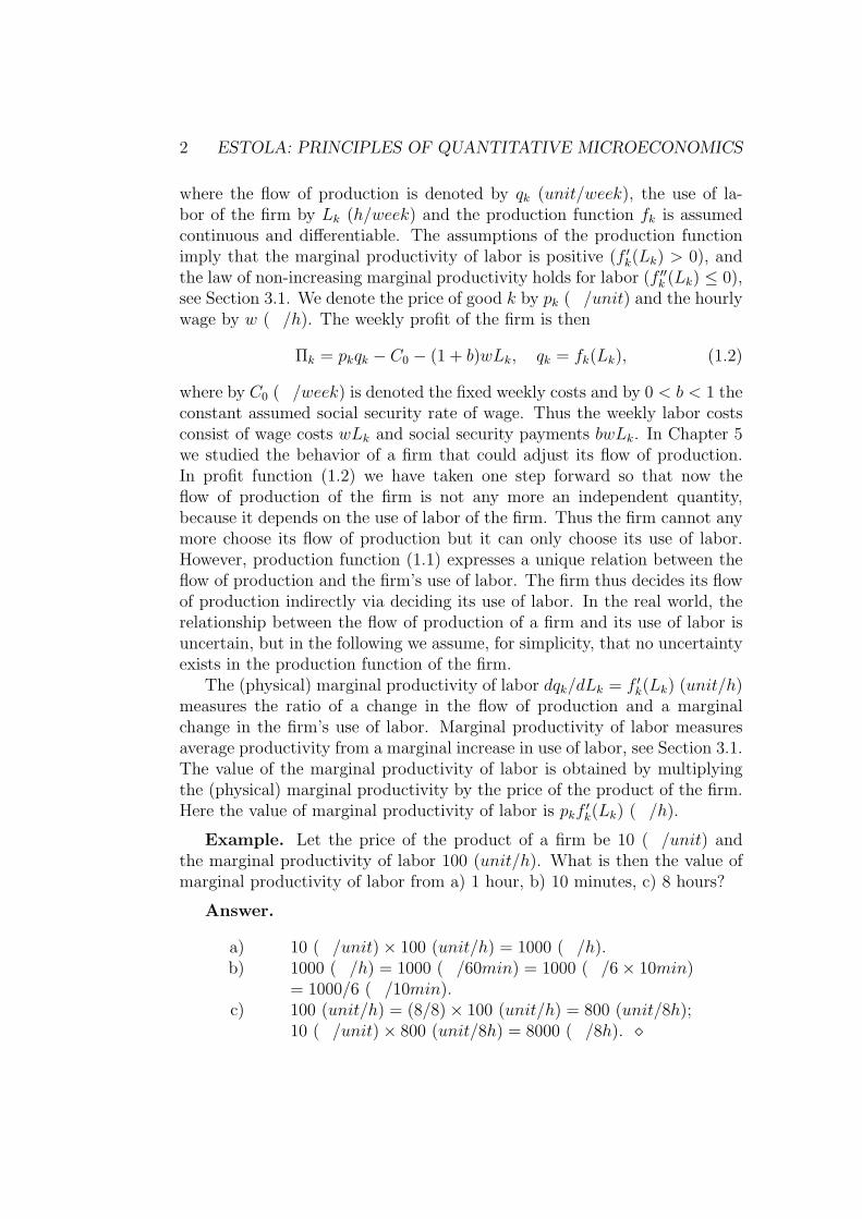
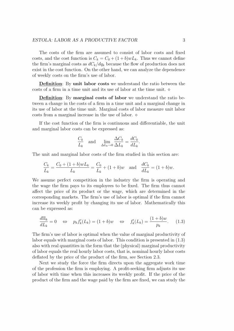
Figure 7.1. The demand of labor of a firm
The relation w = pkf′k
(Lk(t)
)/(1 + b), that defines the equilibrium use of
labor of the firm, is called the demand relation of labor of this firm. Itshows the firm’s optimal use of labor at different wage levels, see Figure 7.1.The slope of the labor demand function in coordinates (Lk, w),
dw
dLk
=pkf
′′k (Lk)
1 + b≤ 0,
depends on the non-increasing marginal productivity of labor. From thedemand relation of labor we see that an increase in price pk moves the labor

ESTOLA: LABOR AS A PRODUCTIVE FACTOR 5
demand relation upward (or ‘right’) in the coordinate system (Lk, w). Theuse of labor of the firm thus depends on the price of the product of the firm,which reflects the ‘derived demand’ character of labor.
1.2 *Newtonian Theory of Use of Labor
Applying the force acting upon the use of labor of a firm defined in theprevious section, we can write an equation of motion for the labor input as:
L′k(t) = g(Fd), g′(Fd) > 0, g(0) = 0, Fd = pkf′(Lk(t)
)−(1+b)w, (1.4)
where g is a function with the above characteristics. Function g expressesthe relationship between the acceleration of use of labor L′k(t) (h/week2)and the force acting upon the labor input of the firm. This relationship isasymptotically stable (Section 4.12) if the following inequality holds strictly:
∂L′k(t)
∂Lk
= g′(Fd)× ∂Fd
∂Lk
= g′(Fd)× pkf′′k (Lk)
(1 + b)≤ 0.
Decreasing marginal productivity of labor is thus a sufficient condition forstability. Taking the Taylor series approximation of function g(Fd) in theneighborhood of point Fd = 0, assuming the error term zero and denotingmLk
= 1/g′(0) > 0, Eq. (1.4) takes the form:
mLkL′k(t) = pkf
′k
(Lk(t)
)− (1 + b)w ⇔ L′k(t) =
pkf′k
(Lk(t)
)− (1 + b)w
mLk
.
(1.5)This is the Newtonian equation of motion for the labor input of the firm.
According to (1.5), the firm increases its use of labor if the value ofmarginal productivity of labor exceeds hourly labor costs, and vice versa.We could have added also static friction in Eq. (1.5) to explain that the firmmay not always change its use of labor when the force acting upon it deviatesfrom zero. This, however, is omitted as well as the finding of solutions forthe differential equation (1.5). If an exact functional form is assumed forfunction fk(Lk), the solution of (1.5) defines the time path for Lk(t).
If the equation of motion for the use of labor in (1.5) is solved and sub-stituted in the firm’s production function, the time path of production canbe determined. Even though the exact form of the production function isnot known, and the equation of motion for labor is not solved, the accelera-tion of production can still be modelled by taking the time derivative of theproduction function and substituting there Eq. (1.5) as:
q′k(t) = f ′k(Lk(t)
)L′k(t) = f ′k
(Lk(t)
) [pkf′k
(Lk(t)
)− (1 + b)w]
mLk
.
6 ESTOLA: PRINCIPLES OF QUANTITATIVE MICROECONOMICS
The dynamics of production is thus determined by the firm’s use of labor.
1.3 Labor Supply of a Person
Here we analyze the labor supply of a person as his choice between workand leisure time on the basis of the benefits and costs of this decision. Thesituation is analogous to a consumer’s choice studied in Chapter 4. A laborsupplier makes his decision to supply work time on the basis of his preferencesconcerning working and having leisure time. The compensation from work(wage or salary), and the available time restrict the possible choices of thelabor supplier, similarly as the budget equation does for a consumer.
In most countries, the laws concerning work time limit the daily andweekly work time of an individual. For this reason, the planning time horizonof a labor supplier is assumed long enough so that the number of workinghours can be considered as an adjustable quantity. Due to this, the planningtime horizon of a labor supplier is assumed to be one year. The labor supplier‘chooses’ the number of work hours in a year he would be willing to work atthe hourly wage he believes to be receiving on the average during the year.
We denote the hourly wage as w (�/h), the constant assumed income taxrate by a (a dimensionless number 0 < a < 1), the number of working hoursin a year by L (h/y), and the annual after-tax wage income by T (�/y). ThenT = wL−awL = (1−a)wL, where wL is annual gross wage income and awLannual wage taxes paid. The maximal possible number of working hours ina year is calculated as follows: work 5 days in a week with 8 hours per dayminus annual holiday of 4 weeks. The maximal number of annual workingdays is then: 48 (week/y)×5 (d/week) = 240 (d/y), and the maximal numberof annual working hours is approximately 240 (d/y)× 8 (h/d) = 1920 (h/y).Labor supplier has thus leisure time in a year H (h/y) = 1920 (h/y)−L (h/y)together with week-ends, evenings and nights.
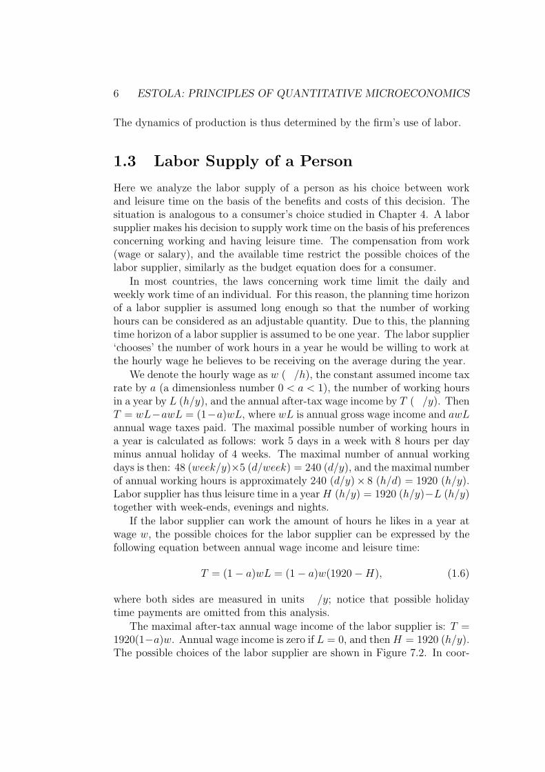
If the labor supplier can work the amount of hours he likes in a year atwage w, the possible choices for the labor supplier can be expressed by thefollowing equation between annual wage income and leisure time:
T = (1− a)wL = (1− a)w(1920−H), (1.6)
where both sides are measured in units �/y; notice that possible holidaytime payments are omitted from this analysis.
The maximal after-tax annual wage income of the labor supplier is: T =1920(1−a)w. Annual wage income is zero if L = 0, and then H = 1920 (h/y).The possible choices of the labor supplier are shown in Figure 7.2. In coor-

ESTOLA: LABOR AS A PRODUCTIVE FACTOR 7
dinate system (H,T ) the slope of the ‘budget line’ of the labor supplier is:dT/dH = −(1− a)w < 0; the greater the w, the steeper the line.
Figure 7.2. The possible choices of a labor supplier
A labor supplier enjoys income and leisure time, and the law of non-increasing marginal utility is assumed to hold for both these ‘goods’. Theutility function of a labor supplier could be derived from a set of axiomslike that of a consumer. However, we omit this and assume that the utilityof a labor supplier is measured by continuous and differentiable function
u = u(H,T ),∂u(H,T )
∂H> 0,
∂u(H,T )
∂T> 0,
∂2u(H,T )
∂H2≤ 0,
∂2u(H,T )
∂T 2≤ 0,
∂2u(H,T )
∂T∂H=∂2u(H,T )
∂H∂T;
the first order partials are the corresponding marginal utilities, the non-positivity of the second order partials with respect to the same quantityimply non-increasing marginal utility; the second order cross partials areequal due to the assumed continuity of the partial functions.
The arguments of the utility function of a labor supplier are annual after-tax wage income and leisure time. Utility thus consists of different factorsthan that of a consumer who gains utility from the consumption of goods.The satisfaction from leisure time can though be understood to be gainedfrom the ‘consumption’ of leisure time, but receiving wage income hardlycan be understood as some kind of consumption. In his decision-making,the labor supplier compares the satisfaction from leisure time and its alter-native cost, the lost income due to not working. In this way the situationcorresponds to that of a consumer. The measurement unit of utility does notagain have an essential role in the modelling. Utility is again an auxiliaryquantity needed in defining the willingness-to-pay of the labor supplier forleisure time. Thus we set the measurement unit for utility as ut/y.
Figure 7.3. An indifference curve of a labor supplier
The preferences of a labor supplier can be described by indifference curves,see Figure 7.3. One indifference curve expresses constant utility, and the slopeof an indifference curve in coordinates (H,T ) can be derived as (Section 4.6):
du = 0 ⇔ ∂u
∂HdH +
∂u
∂TdT = 0 ⇒ dT
dH= −
∂u(H,T )∂H
∂u(H,T )∂T
< 0.
The law of non-increasing marginal utility makes the indifference curves up-ward convex in Figure 7.3. The greater the annual leisure time of a la-bor supplier, the smaller his marginal utility ∂u(H,T )
∂Hand the less steep the
8 ESTOLA: PRINCIPLES OF QUANTITATIVE MICROECONOMICS
curve. The greater the annual after-tax wage income of the labor supplier,the smaller his marginal utility ∂u(H,T )
∂Tand the more steep the curve.
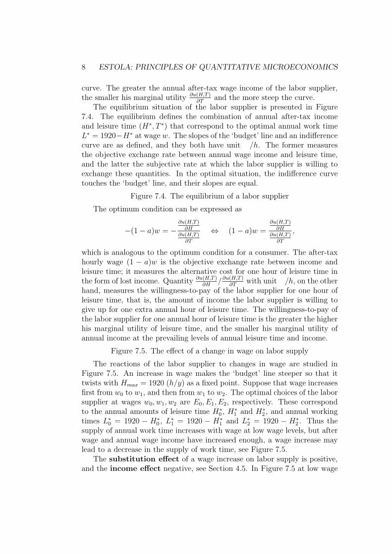
The equilibrium situation of the labor supplier is presented in Figure7.4. The equilibrium defines the combination of annual after-tax incomeand leisure time (H∗, T ∗) that correspond to the optimal annual work timeL∗ = 1920−H∗ at wage w. The slopes of the ‘budget’ line and an indifferencecurve are as defined, and they both have unit �/h. The former measuresthe objective exchange rate between annual wage income and leisure time,and the latter the subjective rate at which the labor supplier is willing toexchange these quantities. In the optimal situation, the indifference curvetouches the ‘budget’ line, and their slopes are equal.
Figure 7.4. The equilibrium of a labor supplier
The optimum condition can be expressed as
−(1− a)w = −∂u(H,T )
∂H∂u(H,T )
∂T
⇔ (1− a)w =∂u(H,T )
∂H∂u(H,T )
∂T
,
which is analogous to the optimum condition for a consumer. The after-taxhourly wage (1 − a)w is the objective exchange rate between income andleisure time; it measures the alternative cost for one hour of leisure time inthe form of lost income. Quantity ∂u(H,T )
∂H/∂u(H,T )
∂Twith unit �/h, on the other
hand, measures the willingness-to-pay of the labor supplier for one hour ofleisure time, that is, the amount of income the labor supplier is willing togive up for one extra annual hour of leisure time. The willingness-to-pay ofthe labor supplier for one annual hour of leisure time is the greater the higherhis marginal utility of leisure time, and the smaller his marginal utility ofannual income at the prevailing levels of annual leisure time and income.
Figure 7.5. The effect of a change in wage on labor supply
The reactions of the labor supplier to changes in wage are studied inFigure 7.5. An increase in wage makes the ‘budget’ line steeper so that ittwists with Hmax = 1920 (h/y) as a fixed point. Suppose that wage increasesfirst from w0 to w1, and then from w1 to w2. The optimal choices of the laborsupplier at wages w0, w1, w2 are E0, E1, E2, respectively. These correspondto the annual amounts of leisure time H∗0 , H∗1 and H∗2 , and annual workingtimes L∗0 = 1920 − H∗0 , L∗1 = 1920 − H∗1 and L∗2 = 1920 − H∗2 . Thus thesupply of annual work time increases with wage at low wage levels, but afterwage and annual wage income have increased enough, a wage increase maylead to a decrease in the supply of work time, see Figure 7.5.
The substitution effect of a wage increase on labor supply is positive,and the income effect negative, see Section 4.5. In Figure 7.5 at low wage
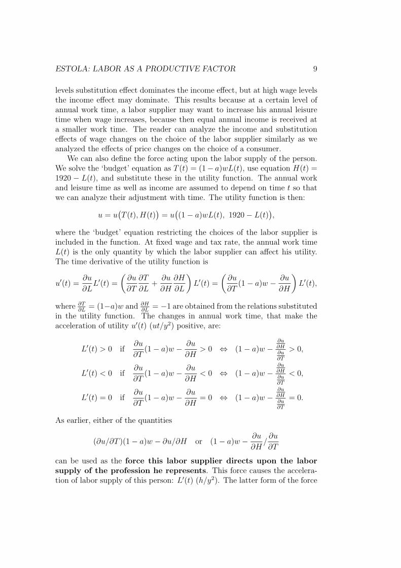
ESTOLA: LABOR AS A PRODUCTIVE FACTOR 9
levels substitution effect dominates the income effect, but at high wage levelsthe income effect may dominate. This results because at a certain level ofannual work time, a labor supplier may want to increase his annual leisuretime when wage increases, because then equal annual income is received ata smaller work time. The reader can analyze the income and substitutioneffects of wage changes on the choice of the labor supplier similarly as weanalyzed the effects of price changes on the choice of a consumer.
We can also define the force acting upon the labor supply of the person.We solve the ‘budget’ equation as T (t) = (1− a)wL(t), use equation H(t) =1920 − L(t), and substitute these in the utility function. The annual workand leisure time as well as income are assumed to depend on time t so thatwe can analyze their adjustment with time. The utility function is then:
u = u(T (t), H(t)
)= u
((1− a)wL(t), 1920− L(t)
),
where the ‘budget’ equation restricting the choices of the labor supplier isincluded in the function. At fixed wage and tax rate, the annual work timeL(t) is the only quantity by which the labor supplier can affect his utility.The time derivative of the utility function is
u′(t) =∂u
∂LL′(t) =
(∂u
∂T
∂T
∂L+∂u
∂H
∂H
∂L
)L′(t) =
(∂u
∂T(1− a)w − ∂u
∂H
)L′(t),
where ∂T∂L
= (1−a)w and ∂H∂L
= −1 are obtained from the relations substitutedin the utility function. The changes in annual work time, that make theacceleration of utility u′(t) (ut/y2) positive, are:
L′(t) > 0 if∂u
∂T(1− a)w − ∂u
∂H> 0 ⇔ (1− a)w −
∂u∂H∂u∂T
> 0,
L′(t) < 0 if∂u
∂T(1− a)w − ∂u
∂H< 0 ⇔ (1− a)w −
∂u∂H∂u∂T
< 0,
L′(t) = 0 if∂u
∂T(1− a)w − ∂u
∂H= 0 ⇔ (1− a)w −
∂u∂H∂u∂T
= 0.
As earlier, either of the quantities
(∂u/∂T )(1− a)w − ∂u/∂H or (1− a)w − ∂u
∂H/∂u
∂T
can be used as the force this labor supplier directs upon the laborsupply of the profession he represents. This force causes the accelera-tion of labor supply of this person: L′(t) (h/y2). The latter form of the force
10 ESTOLA: PRINCIPLES OF QUANTITATIVE MICROECONOMICS
consists of the alternative cost of one hour of leisure time, (1 − a)w (�/h),minus the willingness-to-pay of the labor supplier for one hour of leisure time,∂u∂H/ ∂u
∂T(�/h). The equilibrium state (1− a)w = ∂u
∂H/ ∂u
∂Tcorresponds to zero
force. In the equilibrium, the after-tax wage and the willingness-to-pay ofthe labor supplier for one hour of leisure time are equal. This relation ispresented in Figure 7.6 in the form w = (1/(1 − a)) ∂u
∂H/ ∂u
∂T, and it can be
interpreted as the labor supply relation of this person.
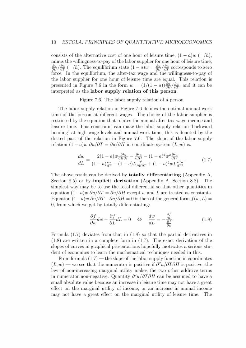
Figure 7.6. The labor supply relation of a person
The labor supply relation in Figure 7.6 defines the optimal annual worktime of the person at different wages. The choice of the labor supplier isrestricted by the equation that relates the annual after-tax wage income andleisure time. This constraint can make the labor supply relation ‘backwardbending’ at high wage levels and annual work time; this is denoted by thedotted part of the relation in Figure 7.6. The slope of the labor supplyrelation (1− a)w ∂u/∂T = ∂u/∂H in coordinate system (L,w) is:
dw
dL=
2(1− a)w ∂2u∂H∂T
− ∂2u∂H2 − (1− a)2w2 ∂2u
∂T 2
(1− a) ∂u∂T− (1− a)L ∂2u
∂H∂T+ (1− a)2wL ∂2u
∂T 2
. (1.7)
The above result can be derived by totally differentiating (Appendix A,Section 8.5) or by implicit derivation (Appendix A, Section 8.8). Thesimplest way may be to use the total differential so that other quantities inequation (1−a)w ∂u/∂T = ∂u/∂H except w and L are treated as constants.Equation (1−a)w ∂u/∂T −∂u/∂H = 0 is then of the general form f(w,L) =0, from which we get by totally differentiating:
∂f
∂wdw +
∂f
∂LdL = 0 ⇔ dw
dL= −
∂f∂L∂f∂w
. (1.8)
Formula (1.7) deviates from that in (1.8) so that the partial derivatives in(1.8) are written in a complete form in (1.7). The exact derivation of theslopes of curves in graphical presentations hopefully motivates a serious stu-dent of economics to learn the mathematical techniques needed in this.
From formula (1.7) — the slope of the labor supply function in coordinates(L,w) — we see that the numerator is positive if ∂2u/∂T∂H is positive; thelaw of non-increasing marginal utility makes the two other additive termsin numerator non-negative. Quantity ∂2u/∂T∂H can be assumed to have asmall absolute value because an increase in leisure time may not have a greateffect on the marginal utility of income, or an increase in annual incomemay not have a great effect on the marginal utility of leisure time. The

ESTOLA: LABOR AS A PRODUCTIVE FACTOR 11
sufficient condition for maximal utility is that ∂2u/∂T∂H > 0. The sign ofthe numerator is thus ambiguous but positive is more plausible.
The first additive term in the denominator of (1.7) is positive, the secondis ambiguous, and the last is non-positive. The greater the annual income T ,the smaller the marginal utility ∂u/∂T . The denominator may thus be neg-ative, i.e. the labor supply relation may be decreasing in coordinate system(L,w) (the backward bending part of the relation corresponds to dw/dL < 0).The probability of this is the higher the greater is T .
In the following we assume ∂2u/∂T∂H > 0 which guarantees the existenceof optimum for the labor supplier. The following results can be derivedfrom the willingness-to-pay of a labor supplier for one hour of leisure time,g(L,w, a) ≡
(∂u∂H/ ∂u
∂T
):
∂g
∂L=
(− ∂2u
∂H2 + ∂2u∂T∂H
(1− a)w)
∂u∂T− ∂u
∂H
(∂2u∂T 2 (1− a)w − ∂2u
∂H∂T
)(
∂u∂T
)2 > 0,
∂g
∂w=
(1− a)L(
∂2u∂T∂H
∂u∂T− ∂u
∂H∂2u∂T 2
)(
∂u∂T
)2 > 0,
∂g
∂a= −
wL(
∂2u∂T∂H
∂u∂T− ∂u
∂H∂2u∂T 2
)(1− a)
(∂u∂T
)2 < 0.
These results imply that the labor supplier is the more willing-to-pay for onehour of leisure time the higher are w and L, and the smaller is a.
1.4 *Newtonian Theory of Labor Supply
According to the force a single labor supplier directs upon the labor supplyof his profession defined in the previous section, we can present the followingequation of motion for his labor supply:
L′(t) = f(Fs), f ′(Fs) > 0, f(0) = 0, Fs = (1− a)w −∂u∂H∂u∂T
, (1.9)
where f is a function with the above properties. Function f expresses therelation between the acceleration of labor supply L′(t) and the force Fs actingupon it (s refers to supply). This relation is asymptotically stable if
∂L′(t)
∂L= f ′(Fs)×
[ ∂u∂T
(∂2u∂H2 − (1− a)w ∂2u
∂H∂T
)+ ∂u
∂H
((1− a)w ∂2u
∂T 2 − ∂2u∂T∂H
)(
∂u∂T
)2
]

12 ESTOLA: PRINCIPLES OF QUANTITATIVE MICROECONOMICS
is negative. The sufficient condition for stability is thus ∂2u/∂H∂T > 0,which is the sufficient condition for maximal utility of the labor supplier.
Taking the first order Taylor series approximation of function f in (1.9) inthe neighborhood of point Fs = 0, assuming the error-term zero and denotingthe ‘inertial ‘mass’ of labor supply’ by mL = 1/f ′(0) > 0, we get:
mLL′(t) = (1− a)w −
∂u∂H∂u∂T
⇔ L′(t) =1
mL
((1− a)w −
∂u∂H∂u∂T
). (1.10)
This is the Newtonian equation of motion for the labor supply of this person.According to Eq. (1.10), the annual labor supply of this person increases ifthe after-tax wage income from one hour is greater than the value of onehour of leisure time for him, and vice versa. We could have added also staticfriction in Eq. (1.10) to explain that labor supply is not always changed whenthe force acting upon it deviates from zero. This, however, is omitted as wellas the finding of possible solutions for the differential equation (1.10).
1.5 Atomistic Labor Market
In Section 7.6 we will analyze the determination of wage and employment ofa profession in a region where all labor suppliers are members of one tradeunion, and the union operates as the wage setter in the labor market. Herewe analyze, on the other hand, the determination of wage and employmentof a profession in a region where every person and firm employing theseworkers behave independently. No trade union exists in the labor marketthat would participate in the wage negotiation, and no minimum wage existsfor the profession. The differences between these two labor market situationscorrespond to those between industries with different kind of competition.
The labor suppliers of the profession we study here are assumed to behomogenous with respect to productivity; differences may exist in personalexchange rates between annual wage income and leisure time. Firms em-ploying the labor of this profession may deviate in their production methodsexpressed by their production functions. If every labor supplier and deman-der operates separately, and both types of partners are numerous, perfectcompetition prevails in the labor market. One supplier (trade union) situa-tion in a labor market corresponds to a monopoly firm in the industry.
Definition: By the demand of labor of a profession in a regionwe understand the aggregate uses of labor of this profession in a time unitat different wages that corresponds to the equilibrium states of every firm inthe region employing labor of this profession. �
ESTOLA: LABOR AS A PRODUCTIVE FACTOR 13
Definition: By the supply of labor of a certain profession in aregion we understand the aggregate work time of laborers of this professionin a time unit at different wages that correspond to the equilibrium states ofevery labor supplier of this profession in the region. �
The above definitions assume that labor markets work locally; a limitedarea exists around firms and homes of labor suppliers that define the maxi-mum distance for daily working. In the above definitions we talked generallyabout labor and wage because the use of labor can be measured in differentunits. For example, if the use labor is measured by the number of employeesworking in a time unit, the unit price of labor is the salary of one employee inthe time unit. However, in the following we measure the firms’ use of laborby worked hours in a time unit; unit labor costs are then hourly wage plussocial security payments.
Our analysis here exactly corresponds to that in Section 6.6, and so thepresentation here is a little shorter. Let perfect competition prevail in theproduct markets of every firm employing the studied type of labor as wellas in the labor market. Let there be n firms employing the type of labor westudy and m labor suppliers. The planning time horizon of every firm andlabor supplier is assumed to be one year.
The modelling of firms’ behavior bases on the assumption that firms try toincrease their annual profit by adjusting their use of labor. Labor suppliersare, similarly, assumed to seek for utility by changing their annual worktime. A firm is assumed to increase its annual use of labor if it believes thatthe revenues from extra production due to the extra work time exceed theextra labor costs, and vice versa. Similarly, an individual labor supplier isassumed to increase his annual work time if the extra income received fromthis exceeds its alternative cost, the decrease in leisure time, and vice versa.
The profit and utility functions of firms and labor suppliers are assumedcontinuous and differentiable, and both parties are assumed to considerchanges in their annual use of labor and work time. With these assump-tions, we can define the forces by which the firms and labor suppliersact upon the annual aggregate work time of this profession.
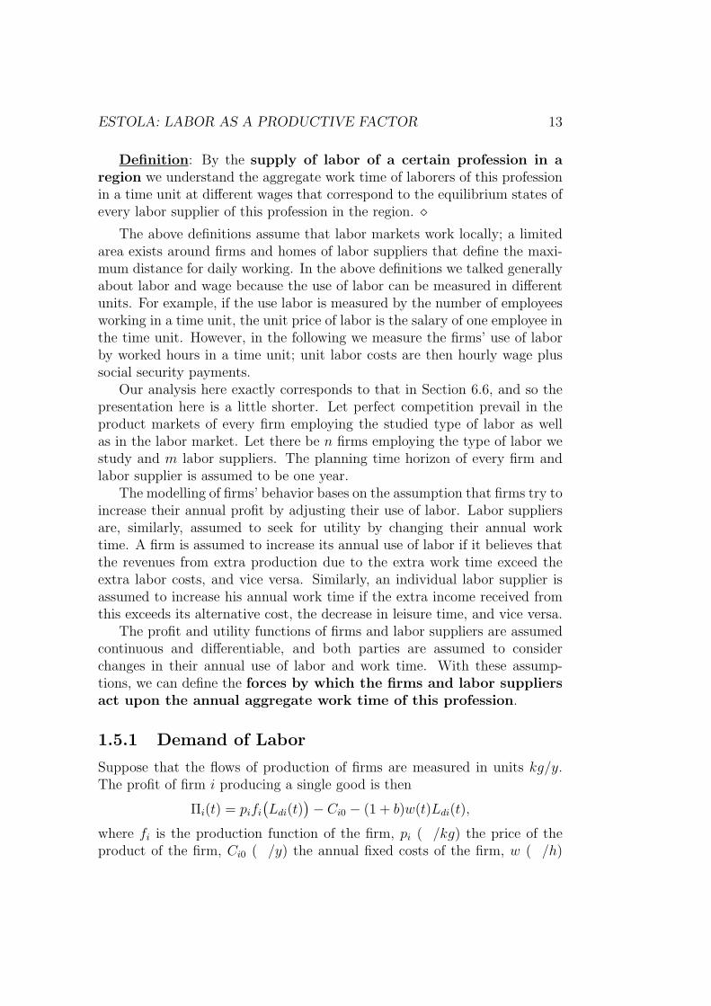
1.5.1 Demand of Labor
Suppose that the flows of production of firms are measured in units kg/y.The profit of firm i producing a single good is then
Πi(t) = pifi
(Ldi(t)
)− Ci0 − (1 + b)w(t)Ldi(t),
where fi is the production function of the firm, pi (�/kg) the price of theproduct of the firm, Ci0 (�/y) the annual fixed costs of the firm, w (�/h)
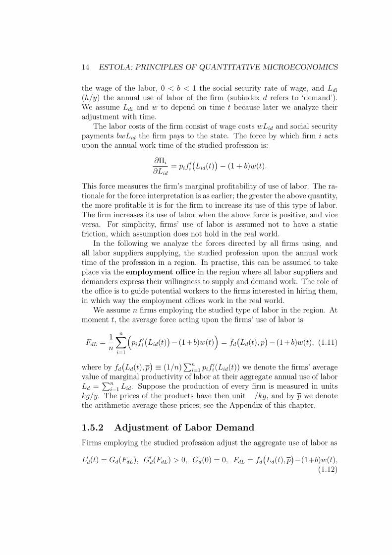
14 ESTOLA: PRINCIPLES OF QUANTITATIVE MICROECONOMICS
the wage of the labor, 0 < b < 1 the social security rate of wage, and Ldi
(h/y) the annual use of labor of the firm (subindex d refers to ‘demand’).We assume Ldi and w to depend on time t because later we analyze theiradjustment with time.
The labor costs of the firm consist of wage costs wLid and social securitypayments bwLid the firm pays to the state. The force by which firm i actsupon the annual work time of the studied profession is:
∂Πi
∂Lid
= pif′i
(Lid(t)
)− (1 + b)w(t).
This force measures the firm’s marginal profitability of use of labor. The ra-tionale for the force interpretation is as earlier; the greater the above quantity,the more profitable it is for the firm to increase its use of this type of labor.The firm increases its use of labor when the above force is positive, and viceversa. For simplicity, firms’ use of labor is assumed not to have a staticfriction, which assumption does not hold in the real world.
In the following we analyze the forces directed by all firms using, andall labor suppliers supplying, the studied profession upon the annual worktime of the profession in a region. In practise, this can be assumed to takeplace via the employment office in the region where all labor suppliers anddemanders express their willingness to supply and demand work. The role ofthe office is to guide potential workers to the firms interested in hiring them,in which way the employment offices work in the real world.
We assume n firms employing the studied type of labor in the region. Atmoment t, the average force acting upon the firms’ use of labor is
FdL =1
n
n∑i=1
(pif′i
(Lid(t)
)− (1+ b)w(t)
)= fd
(Ld(t), p
)− (1+ b)w(t), (1.11)
where by fd
(Ld(t), p
)≡ (1/n)
∑ni=1 pif
′i(Lid(t)) we denote the firms’ average
value of marginal productivity of labor at their aggregate annual use of laborLd =
∑ni=1 Lid. Suppose the production of every firm is measured in units
kg/y. The prices of the products have then unit �/kg, and by p we denotethe arithmetic average these prices; see the Appendix of this chapter.
1.5.2 Adjustment of Labor Demand
Firms employing the studied profession adjust the aggregate use of labor as
L′d(t) = Gd(FdL), G′d(FdL) > 0, Gd(0) = 0, FdL = fd
(Ld(t), p
)−(1+b)w(t),
(1.12)
ESTOLA: LABOR AS A PRODUCTIVE FACTOR 15
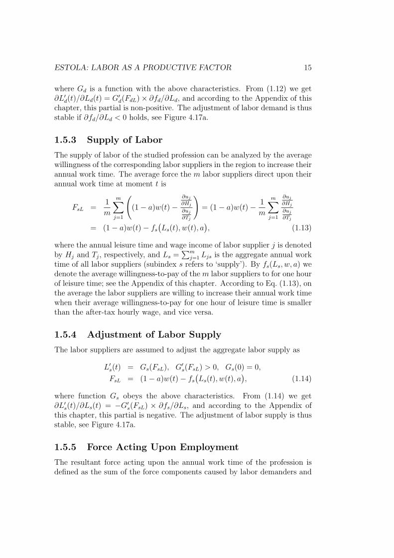
where Gd is a function with the above characteristics. From (1.12) we get∂L′d(t)/∂Ld(t) = G′d(FdL)× ∂fd/∂Ld, and according to the Appendix of thischapter, this partial is non-positive. The adjustment of labor demand is thusstable if ∂fd/∂Ld < 0 holds, see Figure 4.17a.
1.5.3 Supply of Labor
The supply of labor of the studied profession can be analyzed by the averagewillingness of the corresponding labor suppliers in the region to increase theirannual work time. The average force the m labor suppliers direct upon theirannual work time at moment t is
FsL =1
m
m∑j=1
((1− a)w(t)−
∂uj
∂Hj
∂uj
∂Tj
)= (1− a)w(t)− 1
m
m∑j=1
∂uj
∂Hj
∂uj
∂Tj
= (1− a)w(t)− fs
(Ls(t), w(t), a
), (1.13)
where the annual leisure time and wage income of labor supplier j is denotedby Hj and Tj, respectively, and Ls =
∑mj=1 Ljs is the aggregate annual work
time of all labor suppliers (subindex s refers to ‘supply’). By fs(Ls, w, a) wedenote the average willingness-to-pay of the m labor suppliers to for one hourof leisure time; see the Appendix of this chapter. According to Eq. (1.13), onthe average the labor suppliers are willing to increase their annual work timewhen their average willingness-to-pay for one hour of leisure time is smallerthan the after-tax hourly wage, and vice versa.
1.5.4 Adjustment of Labor Supply
The labor suppliers are assumed to adjust the aggregate labor supply as
L′s(t) = Gs(FsL), G′s(FsL) > 0, Gs(0) = 0,
FsL = (1− a)w(t)− fs
(Ls(t), w(t), a
), (1.14)
where function Gs obeys the above characteristics. From (1.14) we get∂L′s(t)/∂Ls(t) = −G′s(FsL) × ∂fs/∂Ls, and according to the Appendix ofthis chapter, this partial is negative. The adjustment of labor supply is thusstable, see Figure 4.17a.
1.5.5 Force Acting Upon Employment
The resultant force acting upon the annual work time of the profession isdefined as the sum of the force components caused by labor demanders and
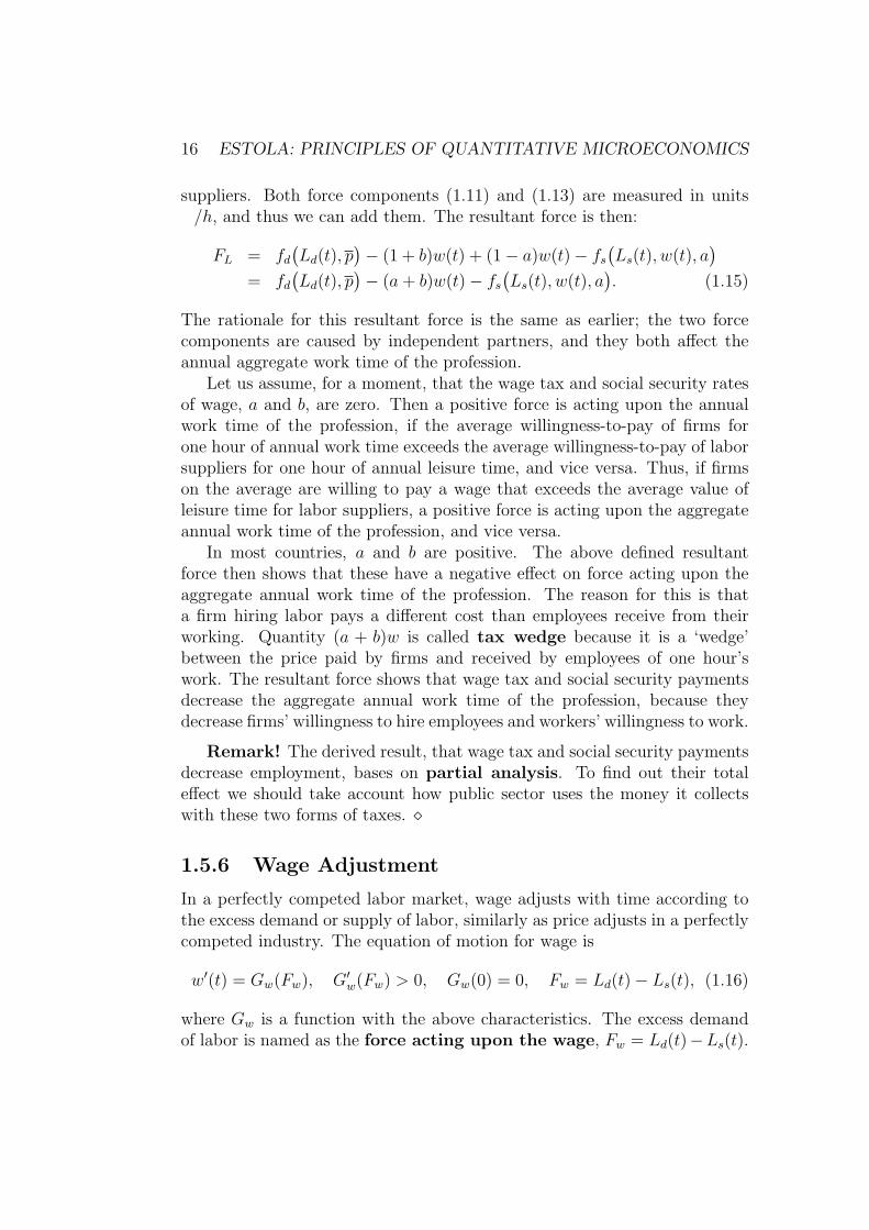
16 ESTOLA: PRINCIPLES OF QUANTITATIVE MICROECONOMICS
suppliers. Both force components (1.11) and (1.13) are measured in units�/h, and thus we can add them. The resultant force is then:
FL = fd
(Ld(t), p
)− (1 + b)w(t) + (1− a)w(t)− fs
(Ls(t), w(t), a
)= fd
(Ld(t), p
)− (a+ b)w(t)− fs
(Ls(t), w(t), a
). (1.15)
The rationale for this resultant force is the same as earlier; the two forcecomponents are caused by independent partners, and they both affect theannual aggregate work time of the profession.
Let us assume, for a moment, that the wage tax and social security ratesof wage, a and b, are zero. Then a positive force is acting upon the annualwork time of the profession, if the average willingness-to-pay of firms forone hour of annual work time exceeds the average willingness-to-pay of laborsuppliers for one hour of annual leisure time, and vice versa. Thus, if firmson the average are willing to pay a wage that exceeds the average value ofleisure time for labor suppliers, a positive force is acting upon the aggregateannual work time of the profession, and vice versa.
In most countries, a and b are positive. The above defined resultantforce then shows that these have a negative effect on force acting upon theaggregate annual work time of the profession. The reason for this is thata firm hiring labor pays a different cost than employees receive from theirworking. Quantity (a + b)w is called tax wedge because it is a ‘wedge’between the price paid by firms and received by employees of one hour’swork. The resultant force shows that wage tax and social security paymentsdecrease the aggregate annual work time of the profession, because theydecrease firms’ willingness to hire employees and workers’ willingness to work.
Remark! The derived result, that wage tax and social security paymentsdecrease employment, bases on partial analysis. To find out their totaleffect we should take account how public sector uses the money it collectswith these two forms of taxes. �
1.5.6 Wage Adjustment
In a perfectly competed labor market, wage adjusts with time according tothe excess demand or supply of labor, similarly as price adjusts in a perfectlycompeted industry. The equation of motion for wage is
w′(t) = Gw(Fw), G′w(Fw) > 0, Gw(0) = 0, Fw = Ld(t)− Ls(t), (1.16)
where Gw is a function with the above characteristics. The excess demandof labor is named as the force acting upon the wage, Fw = Ld(t)−Ls(t).
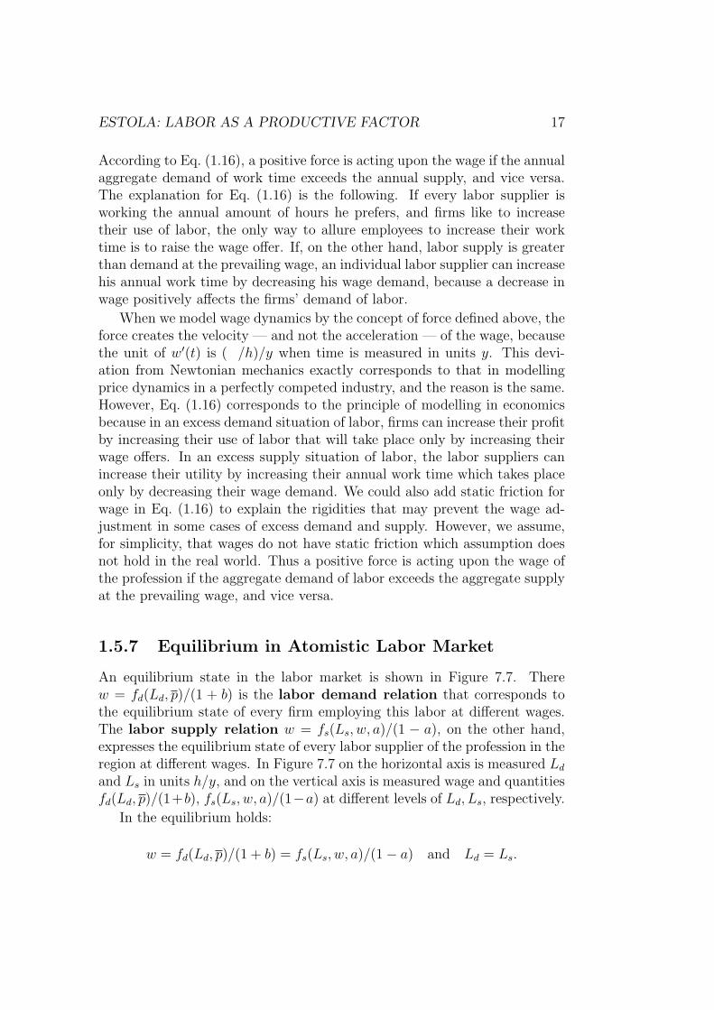
ESTOLA: LABOR AS A PRODUCTIVE FACTOR 17
According to Eq. (1.16), a positive force is acting upon the wage if the annualaggregate demand of work time exceeds the annual supply, and vice versa.The explanation for Eq. (1.16) is the following. If every labor supplier isworking the annual amount of hours he prefers, and firms like to increasetheir use of labor, the only way to allure employees to increase their worktime is to raise the wage offer. If, on the other hand, labor supply is greaterthan demand at the prevailing wage, an individual labor supplier can increasehis annual work time by decreasing his wage demand, because a decrease inwage positively affects the firms’ demand of labor.
When we model wage dynamics by the concept of force defined above, theforce creates the velocity — and not the acceleration — of the wage, becausethe unit of w′(t) is (�/h)/y when time is measured in units y. This devi-ation from Newtonian mechanics exactly corresponds to that in modellingprice dynamics in a perfectly competed industry, and the reason is the same.However, Eq. (1.16) corresponds to the principle of modelling in economicsbecause in an excess demand situation of labor, firms can increase their profitby increasing their use of labor that will take place only by increasing theirwage offers. In an excess supply situation of labor, the labor suppliers canincrease their utility by increasing their annual work time which takes placeonly by decreasing their wage demand. We could also add static friction forwage in Eq. (1.16) to explain the rigidities that may prevent the wage ad-justment in some cases of excess demand and supply. However, we assume,for simplicity, that wages do not have static friction which assumption doesnot hold in the real world. Thus a positive force is acting upon the wage ofthe profession if the aggregate demand of labor exceeds the aggregate supplyat the prevailing wage, and vice versa.
1.5.7 Equilibrium in Atomistic Labor Market
An equilibrium state in the labor market is shown in Figure 7.7. Therew = fd(Ld, p)/(1 + b) is the labor demand relation that corresponds tothe equilibrium state of every firm employing this labor at different wages.The labor supply relation w = fs(Ls, w, a)/(1 − a), on the other hand,expresses the equilibrium state of every labor supplier of the profession in theregion at different wages. In Figure 7.7 on the horizontal axis is measured Ld
and Ls in units h/y, and on the vertical axis is measured wage and quantitiesfd(Ld, p)/(1+b), fs(Ls, w, a)/(1−a) at different levels of Ld, Ls, respectively.
In the equilibrium holds:
w = fd(Ld, p)/(1 + b) = fs(Ls, w, a)/(1− a) and Ld = Ls.
18 ESTOLA: PRINCIPLES OF QUANTITATIVE MICROECONOMICS
Definition: In the equilibrium of an atomistic labor market, the forcesacting upon the demand, supply, and the wage of the profession vanish. �
Figure 7.7. The equilibrium state in a labor market
Remark! The labor demand and supply relations in Figure 7.7 may notcorrespond to the annual uses of labor of the firms, and the annual amountsof work time of the labor suppliers at a certain moment of time, but theydescribe the aggregate amounts of annual work time in the region when everyfirm and labor supplier are in their equilibrium state. The stability analysesgiven earlier show, however, that both parties adjust their behavior with timein order to reach their equilibrium state with time. �
The two non-equilibrium situations in Figure 7.7 can be analyzed as inChapter 6. At wage w1, excess demand Ld1 − Ls1 > 0 of labor prevails, andat wage w2, excess supply Ls2 − Ld2 > 0 prevails. Eq. (1.16) shows thatthe excess demand and supply situations in Figure 7.7 change wage so thatthe labor market settles into its equilibrium. Because the wage adjustmentaccording to excess demand guarantees that the labor market reaches itsequilibrium state with time, the system is stable. The system of differentialequations describing an atomistic labor market exactly corresponds to thatin Section 6.3.2, and it is studied in Section 7.8.1.
1.5.8 Approximation of the Equilibrium
In this section we separate supply and demand by subscripts s, d. Accordingto Sections 7.1 and 7.3, when every firm and labor supplier have adjustedoptimally, we have
(1 + b)w = pif′i(Ldi) and (1− a)w =
∂uj
∂Hj
∂uj
∂Tj
, (1.17)
i = 1, . . . n and j = 1, . . . ,m. Adding the n and m equations in (1.17),separately, and dividing the results by n and m, respectively, we get
(1 + b)w =1
n
n∑i=1
pif′i(Lid), (1− a)w =
1
m
m∑j=1
∂uj
∂Hj
∂uj
∂Tj
. (1.18)
This corresponds to the neoclassical equilibrium in the labor market.
In the Appendix of this chapter we show that we can approximate the
ESTOLA: LABOR AS A PRODUCTIVE FACTOR 19
average of firms’ values of marginal productivity of labor as
F (Ld, p) ≡1
n
n∑i=1
pif′i(Lid) ≈ a0
n+a1
n2Ld +
a2
np,
Ld =n∑
i=1
Lid, p =1
n
n∑i=1
pi, (1.19)
where constants a0 > 0, a1 < 0, a2 > 0 have units �/h, (�× y)/h2 and kg/h,respectively; see the Appendix.
In the Appendix of this chapter, we show that we can approximate thelabor suppliers’ average willingness-to-pay for one hour of leisure time as
G(Ls, w, a) ≡ 1
m
m∑j=1
∂uj
∂Hj
∂uj
∂Tj
≈ b0
m+
b1
m2Ls +
b2
mw +
b3
ma,
where the aggregate labor supply of the m labor suppliers is denoted byLs =
∑mj=1 Lsj, and constants b0 > 0, b1 > 0, b3 < 0 have units �/h,
(�× y)/h2 and �/h, respectively; b2 > 0 is dimensionless.The equilibrium state in the labor market can then be approximated as:
Labor demand: (1 + b)w =a0
n+a1
n2Ld +
a2
np, (1.20)
Labor supply: (1− a)w =b0
m+
b1
m2Ls +
b2
mw +
b3
ma. (1.21)
Assuming pi = pi0 ∀i, we can eliminate p from the system (1.20), (1.21);see the Appendix of this chapter. Then setting Ld = Ls we can solve theequilibrium state in the labor market (w∗, L∗d = L∗s) as:
w∗ =a0b1n− a1m(b0 + ab3)
a1m[b2 + (a− 1)m] + (1 + b)b1n2,
L∗d = L∗s =mn{a0[(1− a)m− b2]− (1 + b)(b0 + ab3)n}
a1m[b2 + (a− 1)m] + (1 + b)b1n2. (1.22)
The units of the constants can be used to check that the solutions are di-mensionally well-defined, i.e. the units of w∗, L∗d are �/h, h/y, respectively.
1.5.9 Adjustment in Labor Market Explicitly*
In Sections 7.5.3-5 we presented the equations of motion for the labor de-mand, supply, and wage in a perfectly competed labor market. By tak-ing the Taylor series approximations of functions Gc in (1.12), (1.14), and

20 ESTOLA: PRINCIPLES OF QUANTITATIVE MICROECONOMICS
(1.16) in the neighborhood of the equilibrium points Fc = 0, c = d, s, w,and assuming the error terms zero, we can approximate the functions asGc(Fc) = G′c(0) × Fc, where G′c(0) are positive constants. Denoting theseconstants as G′c(0) = 1/mLc, c = d, s, w, we can interpret them as ‘inversesof the inertial ‘masses’ mLc of the adjusting quantities’. These in-ertial ‘masses’ measure factors resisting changes in the adjusting quantities,and their measurement units are: �× (y/h)2, �× (y/h)2, and h2/�, respec-tively, when time t has unit y. These units make the equations dimensionallyhomogeneous. The factors resisting wage changes are the existing wage con-tracts, costs from renegotiating wages etc.
The equations of motion for labor demand, supply and wage are then:
mLdL′d(t) = fd(Ld, p)− (1 + b)w,
mLsL′s(t) = (1− a)w − fs(Ls, w, a), (1.23)
mLww′(t) = Ld(t)− Ls(t),
where mLd, mLs and mLw are the inertial ‘masses’ of labor demand, supply,and wage. Assuming fd(Ld, p) and fs(Ls, w, a) as in (1.20), (1.21), and thatpi = pi0 ∀i to eliminate quantity p from the System (1.23), we get:
mLdL′d(t) =
a0
n+a1
n2Ld(t)− (1 + b)w(t),
mLsL′s(t) = (1− a)w(t)− b0
m− b1
m2Ls(t)−
b2
mw(t)− b3
ma, (1.24)
mLww′(t) = Ld(t)− Ls(t).
With certain values for the parameters, System (1.24) is globally stable sothat it will converge with time into the equilibrium state given in (1.22).
The equilibrium state in the labor market can be solved by setting L′d(t) =L′s(t) = w′(t) = 0 in System (1.24), and solving the resulting system ofthree equations with respect to the three endogenous variables. The speed ofadjustment of the system toward the equilibrium state depends on the threeinertial masses and the values of the constants. In this book we concentrateon the equilibrium state, however, and in this it is necessary to know thatthe system is stable and will converge into the equilibrium with time.
Because the analytic solution of System (1.24) is rather complicated, wedemonstrate the solution of the system by the following numerical values:m = n = 10, mLd = mLs = mLw = 1, a = b = 0, a0 = 100, a1 = −10and b1 = 20, b2 = 4. The time paths of the variables Ld, Ls, w are shownin Figure 7.8, where on the horizontal axis is time and on the vertical axisare Ld, Ls and w. The three quantities are presented in the same figure todemonstrate their connections, even though the measurement units of the

ESTOLA: LABOR AS A PRODUCTIVE FACTOR 21
quantities differ. The time path of wage is that below those of Ld, Ls. Thefigure shows that wage increases (decreases) when Ld > Ls (Ld < Ls), andwith t→∞, Ld(t), Ls(t)→ 200/13 = 15.38 and w(t)→ 110/13 = 8.46. Theinitial condition in the solution is: Ld(0) = Ls(0) = 10 and w(0) = 5.
Figure 7.8. The time paths of labor demand, supply andwage in an atomistic labor market
As compared with the static neoclassical analysis, by using System (1.23)we can study the dynamics of the labor market by assuming different kindof time dependencies in quantities fd(Ld, p) and fs(Ls, w, a). On the otherhand, the adjustment process can be studied by solving System (1.24) withvarying the numerical values for the parameters in the model. Concerningthe speed of adjustment, the static neoclassical framework is a special case ofEq. (1.23) with an infinite speed of adjustment, that is, mLc = 0, c = d, s, w.
1.6 Trade Union in Labor Market
In the previous section we analyzed the determination of employment andwage of a profession in a perfectly competed labor market. There the laborsuppliers were not members of a trade union, and the firms were not mem-bers of an employer union. However, in many countries people with certaineducation and work experience belong in a trade union, firms belong in anemployer union, and wage negotiations take place between these unions. Inspite of a wage contract between these unions, every firm and labor suppliermakes their decision whether to hire a person or accept a work offer inde-pendently. These matters make the functioning of the labor market morecomplicated because many of the work contracts are not made at the wageagreed by the unions. Common is that work contracts take place at a higherwage than the unions have agreed. The difference between the contract wageand current wage is called wage slide.
In this section, we analyze the behavior of a unionized labor market by onesimplified model called a Monopoly Union -model. This model assumesthat a trade union makes the choice on behalf of its members with respectto their work time and wage. Let the time horizon be one year. Analogouslywith a monopoly firm, the trade union is supposed to know the demandrelation of its ‘product’ (labor), and the union sets the wage like a monopolyfirm sets the price of its product. Like a monopoly firm, the monopoly unionchooses the optimal (annual use of labor, wage) -combination from the annualaggregate demand relation of its members work time.
The demand of work time of union members is a unique relation between

22 ESTOLA: PRINCIPLES OF QUANTITATIVE MICROECONOMICS
the use of labor of union members and wage. The utility of the union isassumed to depend on the after-tax wage and aggregate annual work time ofunion members. The target function of the monopoly union is
u = u(wN , L
),
∂u
∂wN
> 0,∂u
∂L> 0,
∂2u
∂wN2≤ 0,
∂2u
∂L2≤ 0,
∂2u
∂L∂wN
=∂2u
∂wN∂L, wN = (1− a)w,
where wN (�/h) is the after-tax hourly wage of union members, 0 < a < 1 thewage tax rate, w (�/h) the hourly wage, and L (h/y) the annual aggregatework time of union members. The marginal utilities of after-tax wage andemployment of union members, ∂u/∂wN , ∂u/∂L, are positive, the secondorder partials of the utility function with respect to the same quantity arenon-positive due to the non-increasing marginal utility, and the second ordercross partials are equal due to the continuity of the partial functions.
Remark! Talking about utility function in the connection of a tradeunion is somewhat absurd because a union is not a creature that can feelpleasure or satisfaction. A trade union has goals it aims to reach, and thetarget (utility) function of a union consists of some measures for these goals.Thus when we talk about the utility function of a trade union, we actuallyrefer to the target function that contains the goals of the union. The existenceof a continuous target function for a union should be derived starting from aset of axioms as we did for a consumer. This derivation is, however, omitted,and we assume that the ‘utility’ of a trade union can be measured by acontinuous and differentiable function with unit ut/y. �
Analogously as in consumer theory, we can define a family of indifferencecurves for a monopoly union where one curve represents constant utility.The difference between the utility functions of an individual laborer and atrade union is that a trade union benefits of every rented hour of its members’work time, while a decrease in leisure time decreases the utility of the laborerwhose work time increases. Trade union is thus a macro unit the goals ofwhich cannot be directly added from those of its members.
Union members gain when their leisure time increases other things beingequal, while a union cannot enjoy of leisure time. Union gains of everyrented hour of its members work time in the form of the payments it receivesfrom its members. Unemployed union members, on the other hand, causeexpenditures for the union in the form of unemployment benefits. The higherthe wage the union can rent the work time of its members, and the higherthe share of employed union members, the more the union receives payments,and the more certain the union leaders can be of their re-election.

ESTOLA: LABOR AS A PRODUCTIVE FACTOR 23
The slope of an indifference curve of the trade union in coordinates (L,w)can be derived as follows. The total differential of the utility function is:
du =∂u
∂wN
dwN +∂u
∂LdL.
Then, setting du = 0 in the above formula and substituting there dwN =(1− a)dw from wN = (1− a)w and ∂u/∂wN from
∂u
∂w=
∂u
∂wN
∂wN
∂w= (1− a)
∂u
∂wN
⇔ ∂u
∂wN
=1
(1− a)
∂u
∂w,
we get the slope as:
dw
dL= −
∂u∂L∂u∂w
< 0.
Because the marginal utilities of wage and employment are positive, an in-difference curve is decreasing in coordinate system (L,w).
The existence of a trade union does not affect the demand of labor, andwe assume the labor demand relation of union members as in Section 7.5.2
(1 + b)w = fd(L, p), (1.25)
where subindex d in the use of labor is omitted because here we do not needto separate labor demand and supply. The labor demand relation (1.25)expresses a unique relation between the wage and the annual equilibrium useof labor of every firm employing this labor at different wages. A trade unionin a monopoly position sets the wage for its members, and firms decide theannual work time they will employ at this wage.
Similarly as a monopoly firm, a monopoly union has only one quantityby which it can affect its utility; either the wage or the aggregate annualwork time. If the union likes to get a certain annual work time rented, thedemand relation of the work time of union members shows at which wagethis takes place. If, however, the union likes a certain wage for its members,the demand relation of the work time of union members shows the annualwork time that can be rented at this wage.
The optimal situation of the monopoly union (L∗, w∗) is presentedin Figure 7.9. In the optimum, the slope of an indifference curve is equal tothat of the annual demand relation of work time of union members:
−∂u∂L∂u∂w
=1
(1 + b)
∂fd(L, p)
∂L.

24 ESTOLA: PRINCIPLES OF QUANTITATIVE MICROECONOMICS
This condition — together with the demand relation of annual work time ofunion members — uniquely defines the optimal wage and annual work timeof union members. The equilibrium state is shown in Figure 7.9.
Figure 7.9. The equilibrium of a monopoly union
The force the monopoly union directs upon the annual work time of itsmembers can be derived as follows. We substitute the wage from the utilityfunction of the union by using the labor demand relation as
u = u(wN(t), L(t)) = u
((1− a)
(1 + b)fd
(L(t), p
), L(t)
),
where the aggregate annual work time of union members is set to depend ontime t. The union can then affect its utility only by the annual work timeL(t). The time derivative of the utility function is:
u′(t) =
(∂u
∂wN
(1− a)
(1 + b)
∂fd
(L(t), p
)∂L
+∂u
∂L
)L′(t).
Changes in the aggregate work time, that make the acceleration of utilityu′(t) (ut/y2) positive, are:
L′(t) > 0 if(1− a)
(1 + b)
∂fd
(L(t), p
)∂L
+∂u∂L∂u
∂wN
> 0,
L′(t) < 0 if(1− a)
(1 + b)
∂fd
(L(t), p
)∂L
+∂u∂L∂u
∂wN
< 0,
L′(t) = 0 if(1− a)
(1 + b)
∂fd
(L(t), p
)∂L
+∂u∂L∂u
∂wN
= 0.
As earlier, quantity Fu = (1−a)(1+b)
∂fd(L(t),p)∂L
+ ∂u∂L/ ∂u
∂wNcan be named as the force
the union directs upon the annual work time of union members inthe region. The first negative component in the force measures the decreasein utility due to a decrease in wage required for increasing employment. Thesecond positive component measures the increase in utility due to the increasein annual work time. The union compares the gain of extra work time andits cost, the decrease in wage, and decides the optimal (annual work time,wage) -combination on this basis. The zero force situation corresponds tothe optimal state of the union.
In the above defined force, the measurement unit of utility cancels. Thusthe force is measurable in units (�/h)/(h/y) when the union can quantifythe benefits and losses for the union from this decision. Another way to
ESTOLA: LABOR AS A PRODUCTIVE FACTOR 25
model the decision-making of the trade union is to substitute the aggregateannual employment from the utility function by the labor demand relation,and analyze the utility as a function of the wage. This way we can define aforce the union directs upon the wage of union members. This, however, isomitted because solving the labor demand relation with respect to Ld requiresthe the inverse function of fd that unnecessarily complicates the situation.
1.6.1 Dynamic Trade Union Behavior*
The analysis in the previous section can be expressed mathematically as
L′(t) = f(Fu), f ′(Fu) > 0, f(0) = 0, Fu =(1− a)
(1 + b)
∂fd
(L(t), p
)∂L
+∂u∂L∂u
∂wN
,
where the union is assumed to know the ‘force’ Fu acting upon the employ-ment of union members in the region. The union adjusts the employmentaccording to this force with the aim to increase its utility with time. Assum-ing a specific utility function for the union, we could study the stability ofthe model. However, for shortness we omit these analyzes.
1.7 Mathematical Appendix
The first order Taylor series approximation of the value of marginal produc-tivity of labor of firm i in the neighborhood of the point (Lid0, pi0) is
pif′i
(Ldi
)= pi0f
′i
(Ldi0
)+ pi0f
′′i (Ldi0)
(Ldi − Ldi0
)+ f ′i(Ldi0)
(pi − pi0
)+ εi,(1.26)
where εi is the residual term. Assuming εi = 0 and summing over i, we getn∑
i=1
pif′i
(Ldi
)≈
n∑i=1
[pi0f
′i
(Ldi0
)− pi0f
′′i (Ldi0)Ldi0 − f ′i(Ldi0)pi0
]+
n∑i=1
pi0f′′i (Ldi0)Ldi +
n∑i=1
f ′i(Ldi0)pi ≈ a0 +a1
nLd + a2p,
where Ld =∑n
i=1 Ldi, p = (1/n)∑n
i=1 pi and1
a0 =n∑
i=1
[pi0f
′i
(Ldi0
)− pi0f
′′i (Ldi0)Ldi0 − f ′i(Ldi0)pi0
]= −
n∑i=1
pi0f′′i (Ldi0)Ldi0, a1 =
n∑i=1
pi0f′′i (Ldi0), a2 =
n∑i=1
f ′i(Ldi0).
1Because∑n
i=1 cixi = c∑n
i=1 xi +∑n
i=1(ci− c)xi where c = (1/n)∑n
i=1 ci, the approx-imation is the more accurate the less ci or xi vary, i = 1, . . . , n.
26 ESTOLA: PRINCIPLES OF QUANTITATIVE MICROECONOMICS
The units of a0, a1, a2 are �/h, (�× y)/h2, and kg/h, respectively, and ourassumptions of firms’ marginal productivity make a0 ≥ 0, a1 ≤ 0, and a2 > 0.
The Taylor series approximation of gj(Lsj, w, a) ≡ ∂uj
∂Hj/
∂uj
∂Tjin the neigh-
borhood of the equilibrium point zj0 = (Lsj0, w0, a0) is:
gj(Lsj, w, a) = gj(zj0) +∂gj
∂Lsj
(zj0)(Lsj − Lsj0) +∂gj
∂w(zj0)(w − w0)
+∂gj
∂a(zj0)(a− a0) + εj, j = 1, . . . ,m. (1.27)
Assuming εj = 0 ∀j and summing over j, we get2
m∑j=1
gj(Lsj, w, a)
=m∑
j=1
(gj(zj0)− ∂gj
∂Lsj
(zj0)Lsj0 −∂gj
∂w(zj0)w0 −
∂gj
∂a(zj0)a0
)
+m∑
j=1
∂gj
∂Lsj
(zj0)Lsj + wm∑
j=1
∂gj
∂w(zj0) + a
m∑j=1
∂gj
∂a(zj0)
≈ b0 +b1
mLs + b2w + b3a,
where Ls =∑m
j=1 Lsj and
b0 =m∑
j=1
(gj(zj0)− ∂gj
∂Lsj
(zj0)Lsj0 −∂gj
∂w(zj0)w0 −
∂gj
∂a(zj0)a0
),
b1 =m∑
j=1
∂gj
∂Lsj
(zj0), b2 =m∑
j=1
∂gj
∂w(zj0), b3 =
m∑j=1
∂gj
∂a(zj0).
The units of b0, b1, b3 are: �/h, (�× y)/h2, and �/h, respectively, and b2 isdimensionless. Because gj(Lsj, w, a) is positive at every Lsj, w, a, then b0 > 0(let Lsj → Lsj0, w → w0, a→ a0 and εj → 0 ∀j in (1.27)). In Section 7.3 weshowed that ∂gj/∂Lsj > 0, ∂gj/∂w > 0 and ∂gj/∂a < 0; thus b1 > 0, b2 > 0and b3 < 0.
2See the previous footnote.