Chapter 1: Introduction and General Principles - ALL Chapters.pdf · This Introduction Chapter...
233
ICT Sector Guidance built on the GHG Protocol Product Life Cycle Accounting and Reporting Standard Chapter 1: Introduction and General Principles July 2017 This Guidance has been reviewed for conformance with the GHG Protocol Product Standard.
Transcript of Chapter 1: Introduction and General Principles - ALL Chapters.pdf · This Introduction Chapter...

ICT Sector Guidance built on the
GHG Protocol Product Life Cycle Accounting and Reporting Standard
Chapter 1: Introduction and General Principles
July 2017
This Guidance has been reviewed for conformance with the GHG Protocol Product Standard.

Page 1-2
Contents
Chapter 1: Introduction and General Principles ..................................................................................... 1-1 Executive summary: Introduction and general principles ................................................................... 1-3 1.1 Scope and purpose of the ICT Sector Guidance ..................................................................... 1-4
1.1.1 Current state of the art .................................................................................................... 1-5 1.1.2 Evolving technology ........................................................................................................ 1-5 1.1.3 Building block approach ................................................................................................... 1-6 1.1.4 Product comparisons ....................................................................................................... 1-6 1.1.5 Enabling effect of ICT — avoided emissions ...................................................................... 1-6
1.2 Goals for assessing GHG emissions of ICT products ............................................................... 1-7 1.3 Questions and concerns related to ICT ................................................................................. 1-7 1.4 How this Guidance was developed........................................................................................ 1-8 1.5 How to use this ICT Sector Guidance .................................................................................... 1-9
1.5.1 Who should use this ICT Sector Guidance ......................................................................... 1-9 1.5.2 Structure of this ICT Sector Guidance ............................................................................... 1-9 1.5.3 Key drivers for each chapter .......................................................................................... 1-10
1.6 Related standards ............................................................................................................. 1-11 1.6.1 Generic product LCA standards ...................................................................................... 1-11 1.6.2 GHG Protocol Scope 3 Standard ..................................................................................... 1-12 1.6.3 ICT-specific LCA standards ............................................................................................. 1-13
1.7 General principles and fundamentals of GHG assessments for ICT products........................... 1-13 1.7.1 Principles and appropriateness ....................................................................................... 1-13 1.7.2 Life Cycle Stages ........................................................................................................... 1-13 1.7.3 Screening assessment ................................................................................................... 1-14 1.7.4 Significance .................................................................................................................. 1-15
1.8 ICT-specific commentary on the Product Standard............................................................... 1-16 1.8.1 Scope definition ............................................................................................................ 1-16 1.8.2 Boundary setting ........................................................................................................... 1-17 1.8.3 Data collection and data quality...................................................................................... 1-19 1.8.4 Allocation ..................................................................................................................... 1-20 1.8.5 Assessing uncertainty .................................................................................................... 1-21 1.8.6 Calculating inventory results .......................................................................................... 1-22 1.8.7 Assurance ..................................................................................................................... 1-25 1.8.8 Reporting requirements ................................................................................................. 1-26
Annex: References and Glossary..........................................................................................................A-1
Acknowledgements.............................................................................................................................K-1
Tables
Table 1.1. Examples of functional units ............................................................................................ 1-17
Table 1.2a. Attributable processes to be included within the boundary definition ................................... 1-18
Table 1.2b. Non-attributable processes that may be excluded from the boundary definition....................1-18
Table 1.3. Types of uncertainty and corresponding sources ............................................................... 1-21
Figures
Figure 1.1. Chapter structure ........................................................................................................... 1-10
Figure 1.2. Relationship of ICT Sector Guidance to generic product LCA standards ............................... 1-12
Figure 1.3. Life cycle stages of a product .......................................................................................... 1-14

Page 1-3
Executive summary: Introduction and general principles
This ICT Sector Guidance provides guidance and accounting methods for the calculation of GHG
(greenhouse gas) emissions for ICT (Information and Communication Technology) products with a focus on
ICT services. This ICT Sector Guidance is built on, and in conformance with, the GHG Protocol Product
Standard.1
The ICT Sector Guidance includes the following chapters:
Telecommunications Network Services
Desktop Managed Services
Cloud and Data Center Services
Hardware
Software
Transport Substitution2
This Introduction Chapter gives some context and background to the issues around measuring the GHG
emissions of ICT products, and discusses some of the reasons for doing this.
It also provides an overview of the other chapters and general guidance on the following topics when
assessing ICT products: screening, significance, scope definition, boundary setting, data collection and data
quality, allocation, uncertainty, calculating GHG emissions, assurance, reporting.
Assessing the GHG emissions of ICT products presents a number of challenges because of the nature of ICT,
with the complex and extensive features of ICT services, the long and complex supply chains for ICT
hardware, and the wide use of shared resources within ICT systems requiring specific allocation techniques.
This ICT Sector Guidance aims to address these issues by providing practical methodologies, which provide
a consistent approach to calculating the GHG emissions from ICT goods and services.
1Greenhouse Gas Protocol, “Product Life Cycle Accounting and Reporting Standard,” 2011, available at http://www.ghgprotocol.org/standards/product-standard 2 Note: The Transport Substitution chapter will be published at a later date as an appendix.

Page 1-4
1.1 Scope and purpose of the ICT Sector Guidance This ICT Sector Guidance is published as Sector Guidance built on the GHG Protocol Product Accounting and
Reporting Standard (referred to as the Product Standard throughout this Sector Guidance).
The purpose of this Sector Guidance, which is in conformance with the Product Standard, is to provide
additional guidance to practitioners who are implementing the Product Standard for ICT products (including
ICT services). This Sector Guidance follows a life cycle approach to the assessment of ICT products
(including services).
ICT (information and communication technology) in this Sector Guidance follows the OECD definition,3 which
has the following guiding principle:
“ICT products must primarily be intended to fulfill or enable the function of information processing
and communication by electronic means, including transmission and display.”
The OECD definition includes the following 10 broad categories for ICT products:
Computers and peripheral equipment
Communication equipment
Consumer electronic equipment
Miscellaneous ICT components and goods
Manufacturing services for ICT equipment
Business and productivity software and licensing services
Information technology consultancy and services
Telecommunications services
Leasing or rental services for ICT equipment
Other ICT services.
The Product Standard defines products to be both goods and services, thus for the ICT sector it covers both
physical ICT equipment and delivered ICT services. This Sector Guidance, however, focuses more on the
assessment of ICT services. In this Sector Guidance the definition of products includes both networks and
software as ICT services.
The need for this Sector Guidance is due to the specific nature of ICT products. ICT equipment is
characterized by extensive bills of material (BOM) consisting of hundreds of individual components with long
and complex global supply chains, often using multiple and alternative sources. This makes it inherently
challenging to execute a detailed life cycle assessment (LCA) for typical ICT equipment. The ICT sector is
also characterized by a large number of extensive services. These services are generally complex solutions
including potentially thousands of items of ICT equipment and have significant use stages. In other words,
understanding the use profile and behavioral aspects of the use of the service are important in assessing the
service. Although LCA and the Product Standard are applicable to both goods and services, they are more
easily applied to physical goods because services are intrinsically more complex; it is, therefore, more
complex to assess services. This Sector Guidance seeks to address this, and therefore has specific focus on
the assessment of ICT services.
3 Organisation for Economic Co-operation and Development (OECD), “Information Economy Product Definitions Based on the Central Product Classification (Version 2),” In OECD Digital Economy Papers, No.158, 2009, available at:
http://www.oecd-ilibrary.org/science-and-technology/information-economy-product-definitions-based-on-the-central-product-classification-version-2_222222056845

Page 1-5
This Sector Guidance aims to provide a practical approach to the GHG assessment of ICT products by
providing a consistent and pragmatic approach. While this Sector Guidance is in conformance with the
Product Standard, it provides more details and specificity relevant to the ICT sector. It is important that the
level of precision employed in an assessment matches the goal of the assessment and recognizes the
context in which the results will be interpreted. Therefore this Sector Guidance presents alternative
approaches and estimation techniques, and, where appropriate, provides a hierarchy of approaches. The
specific approach to be taken by the practitioner will depend on the goal of the assessment, the level of
precision required, and the data available (and the associated cost of collecting further data).
ICT products may also have the potential for avoiding GHG emissions through the “enabling effect.” This
ICT Sector Guidance provides guidance for assessing the enabling effect of ICT (see Section 1.1.5 “Enabling
effect of ICT — avoided emissions” in this chapter and, more specifically, in the Transport Substitution
Chapter4).
Thus the purpose of this ICT Sector Guidance is to address the inherent nature of ICT products and
particularly the following points:
Multiple components for ICT equipment
Complex and long supply chains for ICT equipment
Complex nature of ICT services across their life cycle
Often bespoke and tailored characteristics of ICT services to meet specific customer requirements
Allocation of resource use to ICT services, which typically share resources
Significant in-use stage of ICT products
Uncertainty surrounding measurement of use stage
Enabling effect of ICT products
1.1.1 Current state of the art
The ICT industry is very conscious of the impact of ICT in terms of GHG emissions. A number of ICT
companies are performing LCAs and GHG assessments on their products and related research is being
carried out by industry and academia. However, this work is still in development and has limitations. It is far
from routine for ICT companies to automatically carry out GHG assessments on all their products. Generally,
data collection systems cannot readily provide the data needed to carry out an assessment. Reliable and
consistent sources of secondary data and emission factors for ICT components are not easily available.
Reliable data on the actual use of ICT products is also difficult to determine. Therefore, currently, GHG
assessments are typically carried out as individual projects, rather than as a routine business activity. As the
work of measuring GHG emissions continues, it is hoped that more comprehensive datasets will be
developed. These datasets will enable more GHG assessments to be undertaken and for these assessments
to become part of accepted practice in the ICT sector.
1.1.2 Evolving technology
A further significant issue for the ICT sector is the rapidly changing and evolving nature of the technology.
This has a number of potential effects: development of new products; technology being used in new and
unexpected ways; new technologies driving different user and social behaviors; development of more
energy-efficient ICT equipment changing underlying assumptions between in-use and “embodied
emissions”;5 and development of equipment with built-in measurement capabilities (e.g., device energy
consumption, network traffic monitoring and reporting, power saving mode monitoring and reporting). Thus,
4 To be published at a later date. 5 The term “embodied emissions” is defined in Section 1.7.2 “Life Cycle Stages.”

Page 1-6
while this ICT Sector Guidance is intended to be generic in approach, it cannot predict all the potential
changes that will happen in the ICT sector in the coming years.
1.1.3 Building block approach
This Guidance has a strong focus on the assessment of ICT services, and here the approach is to describe
clearly the definition and boundaries of the service, and enumerate the constituent elements that make up
the service. Each constituent element can be considered as a building block and assessed individually, with
the total impact being assessed by summing the impact of all the individual building blocks. This provides for
a consistent and efficient approach. Examples of constituent elements are:
Individual items of ICT equipment
Use of networks
Use of shared equipment (e.g., data centers)
Use of software
Hardware and software maintenance
Help-desk support
1.1.4 Product comparisons
As with the Product Standard, this ICT Sector Guidance is not intended to support product comparisons.
Note that product comparisons are discussed further in the Product Standard (section 1.5). Appendix A of
the Product Standard provides guidance on product comparison and recommends additional specifications
for product comparisons. The Product Standard requires additional product rules to be developed to support
product comparisons, however product rules are outside the scope of this ICT Sector Guidance. See also
section 5.3.2 of the Product Standard for discussion of Product Rules and Sector Guidance.
1.1.5 Enabling effect of ICT — avoided emissions
An “enabling effect” is the opportunity an ICT solution has to avoid GHG emissions in other sectors, which
can be attributed back to the ICT solution as the prime cause of that avoidance.
The Product Standard (sections 11.2 and 11.3.2) states that “avoided emissions shall not be deducted from
the product’s total inventory results, but may be reported separately.” This ICT Sector Guidance follows the
same approach — that avoided GHG emissions caused by an enabling effect shall be reported separately
from the emissions caused directly by a product.
Avoided emissions are defined in the Product Standard as reductions in emissions caused indirectly by a
product, where the product provides the same or similar function as existing products in the marketplace,
but with significantly less GHG emissions.
The Product Standard does not address accounting of avoided emissions, however it was considered
important to include in this ICT Sector Guidance a methodology for assessing the avoided emissions caused
by the enabling effect of ICT, because of the significant potential that ICT has in this area. As this
methodology is different from that for assessing products, it will be included in the Transport Substitution
Chapter as a separate appendix (see Section 1.5.2 “Structure of this ICT Sector Guidance”).
In summary, the methodology provides a comparison of a business-as-usual (BAU) baseline scenario and an
ICT-enabled scenario to demonstrate the benefit of ICT solutions to reduce overall system-level GHG
emissions. This involves calculating the emissions in the following three categories.
ICT Product Emissions
The life cycle emissions of the ICT solution that is causing the enabling effect.
Enabling Effects
The avoided emissions due to the activities avoided as a result of using the ICT solution. These are
further subdivided into immediate enabling effects and longer-term enabling effects.

Page 1-7
Rebound Effects
The increased emissions as a result of using the ICT solution, caused by rebound effects. These
rebound effects may be caused by related consequential effects or by unrelated (and sometimes
unintended) effects and are often related to human behavioral changes. These effects are further
subdivided into immediate rebound effects and longer-term rebound effects. Because of the nature
of rebound effects, assessing them is inherently uncertain as it is difficult to accurately estimate the
effects.
1.2 Goals for assessing GHG emissions of ICT products There are a number of motivations for carrying out a GHG assessment of ICT products. It is important to be
clear what the goal for carrying out an assessment is, what the results will be used for, and who will use the
results. The approach taken for the assessment may well be different depending on the goal.
The Product Standard (chapter 2) identifies some common business goals for companies to carry out a
product life cycle GHG assessment.
For ICT products (including services) the following are typical goals, which this Guidance aims to address:
Understand emissions through the life cycle of the product, and where in the life cycle the majority
of the emissions occur (e.g., understand the proportion of embodied to in-use emissions). This can
help to direct efforts to reduce emissions of the product such as:
Reduction of emissions due to changes in the design of the product
Reduction of emissions due to changes in the manufacture of a good, or provision of a
service
Reduction of emissions in the use stage of a product
Reduction of emissions in response to behavioral changes in the use of the product.
Track changes over time, to monitor the impact of product enhancements and new versions of
products.
Respond to customer questions on the GHG emissions of the product offering.
Public reporting on the GHG emissions of a product (this is required to conform with the Product
Standard).
Each chapter provides further specific examples of goals for the ICT product(s) covered, and where the
Guidance should and should not be used.
1.3 Questions and concerns related to ICT There is a growing interest in ICT with respect to GHG emissions, both because of the significant emissions
associated with the manufacture and use of ICT products, and because of the opportunity for ICT products
to reduce emissions elsewhere (the “enabling effect”). In 2008, the SMART 2020 report6 catalyzed the
debate about the GHG impact of ICT, estimating that ICT is responsible for 2 percent of global GHG
emissions, and also that ICT has the potential to reduce emissions equivalent to five times its own emissions
through the “enabling effect.” The 2012 update, SMARTer 2020,7 estimated that the total emissions from
the ICT industry in 2011 were 0.9 gigatons (Gt) of CO2 equivalent (CO2e) (1.9 percent of all global GHG
emissions), that by 2020, total emissions will be 1.3 gigatons CO2e (2.3 percent of global emissions), and
6 The Climate Group, “SMART 2020: Enabling the Low Carbon Economy in the Information Age,” Global e-Sustainability Initiative (GeSI), 2008, available at http://gesi.org/portfolio/report/69. 7 The Boston Consulting Group (BCG), “SMARTer 2020: The Role of ICT in Driving a Sustainable Future,” Global e-Sustainability Initiative (GeSI), 2012, available at http://gesi.org/SMARTer2020

Page 1-8
that the total abatement potential from ICT solutions by 2020 is seven times its own emissions. In 2015
GeSI published the SMARTer 20308 report, extending the analysis out to 2030. This study predicted that the
global emissions of the ICT sector will be 1.25 Gt CO2e in 2030 (or 1.97% of global emissions), and
emissions avoided through the use of ICT will be 12 Gt CO2e, which is nearly 10 times higher than ICT’s own
emissions.
The following issues and questions are being raised in relation to ICT’s positive and negative impacts on
GHG emissions. This ICT Sector Guidance does not aim to directly answer these questions, but provides
mechanisms and tools with which these issues can be systematically investigated.
Rapid growth of ICT (e.g., driven by use of social networking, smart phones, mobile data usage,
internet usage, internet TV, music and video streaming)
Exponential growth in the use of cloud services and the data centers that support them
Increasing energy efficiency of computing and telecommunications
Social changes driven by ICT
Opportunities to reduce business-related travel through teleworking, telecommuting and remote
collaboration.
Opportunities to indirectly reduce emissions through the use of various smart technologies
Rapid changes in technology and promises of new technology development leading to new
opportunities and challenges
Knowing the best time to replace ICT equipment, considering the improvements in energy efficiency
of new equipment versus the embodied emissions
As ICT equipment becomes more energy efficient, its embodied emissions may become
proportionately more significant than its use-stage emissions
1.4 How this Guidance was developed This Guidance was developed following a collaborative process similar to that used for the development of
GHG Protocol standards. The process was overseen by a 15 person Steering Committee, and the draft
documents were developed by a Technical Working Group of over 50 members representing participating
ICT companies, government bodies, standards developing organizations, NGOs, industry analysts and
academic institutions.
Two rounds of public consultation were held, each with the publication of a draft, and invitation for public
comment, followed by review of the comments and update of the draft. As part of each public consultation,
a series of webinars presented the scope and content of the Guidance. Members of a Stakeholder Advisory
Group (consisting of more than 350 participants from over 45 countries) provided over 700 comments on
both drafts of the Guidance.
Additionally, the World Resources Institute (WRI) reviewed the Guidance providing useful comment and
feedback, and approved it for conformance with the GHG Protocol Product Standard.
No air travel was involved in the making of this Guidance, with all meetings being held remotely using online
collaborative working tools.
8 Accenture Strategy, “SMARTer 2030: ICT Solutions for 21st Century Challenges”, Global e-Sustainability Initiative (GeSI), 2015, available at http://gesi.org/portfolio/project/82

Page 1-9
1.5 How to use this ICT Sector Guidance
1.5.1 Who should use this ICT Sector Guidance
This ICT Sector Guidance is intended primarily for use by practitioners carrying out GHG assessments of ICT
products. Typically this will include practitioners working for a company9 that supplies the ICT product, or a
consultant working on behalf of the company. It may also include researchers carrying out studies in the ICT
sector and customers wishing to understand and reduce the emissions from the ICT products they use.
The ICT Sector Guidance is a supplement to the Product Standard, and thus assumes that the reader is
familiar with the principles and content of the Product Standard. Where appropriate, this guidance document
summarizes and references the Product Standard.
1.5.2 Structure of this ICT Sector Guidance
The ICT Sector Guidance is organized into chapters as shown in Figure 1.1 and described below. Each
chapter covers a specific ICT product (or group of products). Because of the modular (building-block)
approach taken, a chapter is likely to refer to other chapters that cover the product’s constituent elements.
This is particularly true for the chapters covering ICT services.
The chapters in this ICT Sector Guidance do not provide exhaustive cover of all ICT products; the approach
is to prioritize products that have a significant impact in terms of GHG emissions. This Introduction Chapter
(together with the Technical Support chapters) provides generic guidance that can be applied to other areas
of ICT products not explicitly covered in this ICT Sector Guidance. The structure is designed to allow the
addition of more chapters in the future.
This Introduction Chapter provides an overview and general guidance common to GHG assessment of
ICT products.
The Annexes provide common references and a glossary, which are relevant to all the chapters.
The Services Chapters cover ICT services that a company might supply, or a customer might purchase.
These chapters necessarily refer to the Technical Support chapters.
Telecommunications Network Services
Desktop Managed Services
Cloud and Data Center Services
The Technical Support Chapters cover the “infrastructure elements” that are common to most ICT
services.
Hardware
Software
The Appendix covers the use of ICT to avoid GHG emissions in other sectors.
Appendix A – Transport Substitution10
9 The term company is used in this ICT Sector Guidance to represent either a company or an organization that may use the guidance. 10 To be published at a later date.

Page 1-10
Figure 1.1. Chapter structure
As the chapters provide guidance to the Product Standard, they follow the structure of the Product
Standard, using the following headings where appropriate:
Introduction
Goal of the chapter
Business goals for assessing the product
Scope
Functional unit
Boundary setting
Data collection and data quality
Allocation
Calculating inventory results
1.5.3 Key drivers for each chapter
The choice of chapters to include in this guidance has been based on ICT products and services that are
widely adopted and/or may have a significant impact in terms of GHG emissions. The following summarizes
the key drivers behind each chapter:
Telecommunications network services
Telecommunications networks provide the fundamental support to all modern communications. The rapid
growth in the use of the internet, data transfers, mobile communications etc., is leading to significant
increases in associated GHG emissions. At the same time, advances in technologies are leading to more
energy-efficient networks. The aim of the Telecommunications Network Services (TNS) Chapter is to provide
guidance, methodologies, and options to enable practitioners to assess the GHG emissions associated with

Page 1-11
TNS. This helps to identify the relative size and scale of emission sources within different life cycle stages.
Understanding this enables telecommunications providers to communicate and collaborate with suppliers
and customers on ways to reduce GHG emissions.
Desktop managed services
Desktop managed services (DMS) is the provision of computing facilities, usually in a corporate environment.
It is very broad in scope, encompassing the equipment on the customer’s premises (e.g., desktops, laptops,
printers), the data center, the local area network (LAN) and the wide area network (WAN), and the
supporting human services (e.g., break-fix support, help desk). DMS account for a major part of the ICT
sector outsourcing market and a major portion of overall ICT GHG emissions. Customers of DMS are
increasingly demanding accurate and transparent information on the GHG emissions of the DMS provided to
them for reporting purposes and for identification of areas for potential emissions reduction.
Cloud and data center services
Cloud computing, which is a model for efficiently providing ICT services from a shared pool of remote
computing resources (i.e., hardware, data centers, networks, and software applications), can potentially
reduce GHG emissions associated with ICT services. This chapter enables cloud and data center service
providers and customers to report the GHG emissions from cloud and data center services in a consistent
manner and make informed choices to reduce greenhouse gas emissions.
Hardware
ICT hardware is a fundamental component of any ICT system or service. The Hardware Chapter provides
guidance on the GHG assessment of ICT hardware. The methodologies described in the chapter cover
different calculation methods, and provide guidance on different estimation techniques. The chapter also
references other standards that cover the GHG assessment of ICT hardware.
Software
Software has a significant impact on the energy used by ICT hardware (because of both the operating
system and the applications). Thus designing software for energy efficiency can reduce the GHG emissions
of ICT products (including services). This chapter provides software developers and architects guidance to
benchmark and report the GHG emissions from software use in a consistent manner and make informed
choices to reduce greenhouse gas emissions. The chapter is in two parts. Part A provides guidance on the
full life cycle assessment of software, while Part B relates specifically to the energy use of software, and
covers the three categories of software: operating systems (OS), applications, and virtualization.
Transport substitution11
The application of ICT for remote collaboration and remote working (such as teleconferencing and
telecommuting) can reduce GHG emissions in absolute terms by avoiding business travel and employee
commuting. Appendix A “Transport Substitution” provides guidance and methodologies for the calculation
and reporting of the avoided emissions caused by the use of the ICT product.
1.6 Related standards
1.6.1 Generic product LCA standards
This ICT Sector Guidance provides additional guidance for the implementation of the Product Standard for
ICT products. The Product Standard follows a life cycle approach to the GHG assessment of products and
builds on the framework and requirements established in the ISO LCA standards: 14040:2006, Life Cycle
11 To be published at a later date.

Page 1-12
Assessment: Principles and Framework and 14044:2006, Life Cycle Assessment: Requirements and
Guidelines. ISO 14040 and ISO 14044 are considered the base standards for LCA, which other standards are
built on.
Two other generic documents for specifying the life cycle assessment of GHG emissions are the PAS 2050
and the ISO 14067. These documents are applicable to any kind of products, but do not give specific
guidance for ICT products, hence the need for this ICT specific guidance.
The PAS 2050 is a publicly available specification (PAS) for the assessment of life cycle greenhouse gas
emissions of goods and services. It was first published in October 2008 by the British Standards Institution
(BSI), in partnership with the UK Department of Environment Food and Rural Affairs (DEFRA) and the
Carbon Trust. A revised edition (PAS 2050:2011) was released in October 2011.
The ISO technical specification 14067 “Carbon footprint of products -- Requirements and guidelines for
quantification and communication” was published in May 2013.
The relationship between this ICT Sector Guidance and these generic product LCA documents is shown in
Figure 1.2.
All three documents (PAS 2050, Product Standard, and ISO 14067) address the assessment of life cycle GHG
emissions for products, and all are based on ISO 14040 and 14044. Considerable work has been done to
ensure alignment on these three standards through the relevant organizations responsible for developing
them. The revised version of PAS 2050:2011 allows even closer alignment of the Product Standard with the
PAS 2050.
Figure 1.2. Relationship of ICT Sector Guidance to generic product LCA standards
1.6.2 GHG Protocol Scope 3 Standard
The GHG Protocol Scope 3 Standard and the GHG Protocol Product Standard both take a value chain or life
cycle approach to GHG accounting and were developed simultaneously. The Scope 3 Standard accounts for
value chain emissions at the corporate level, while the Product Standard accounts for life cycle emissions at
the individual product level (see section 1.6 of the Product Standard). This ICT Sector Guidance
supplements the Product Standard. However, the methodologies in this guidance are also applicable to
those categories of the scope 3 standard that relate specifically to products, namely:
1. Purchased goods and services
10. Processing of sold products
11. Use of sold products
12. End-of-life treatment of sold products

Page 1-13
1.6.3 ICT-specific LCA standards
Additionally, there are documents published by standards developing organizations (SDOs) that relate to the
life cycle assessment of ICT products. These are all based on the ISO 14040 and 14044 standards. They
provide general requirements for the assessment of ICT products, generally preferring a detailed approach.
The ICT Sector Guidance takes a complementary and more pragmatic perspective to give practitioners more
detailed guidance on how to perform LCAs of ICT products and services. It especially focuses on how to
prioritize and reduce data collection efforts when a less detailed assessment is needed. Special focus is put
on how to define the system boundaries of specific assessment targets.
The ICT-specific LCA standards documents are:
ITU-T L.1410
“Methodology for the assessment of the environmental impact of information and communication
technology goods, networks and services”
(International Telecommunication Union [ITU]. Consented September 2011, published March 2012).
A revision was published in December 2014, which was developed jointly by ITU-T Study Group 5
and ETSI TC EE. The ETSI Standard ETSI ES 203 199 is technically equivalent to the ITU-T L.1410,
and supersedes the previous ETSI TS 103 19912.
IEC TR 62725
“Analysis of quantification methodologies of greenhouse gas emissions for electrical and electronic
products and systems”
(International Electrotechnical Commission [IEC]. Published March 2013).
1.7 General principles and fundamentals of GHG assessments for ICT products
1.7.1 Principles and appropriateness
The principles of product GHG assessments defined in the Product Standard (chapter 4) are as follows:
Relevance
Completeness
Consistency
Transparency
Accuracy
It is important that the approach taken is appropriate to the product being assessed and to how the results
will be used.
1.7.2 Life Cycle Stages
The Product Standard (section 7.2) defines five life cycle stages as follows:
Material acquisition and preprocessing
Production
12 ETSI TS 103 199 “Life Cycle Assessment (LCA) of ICT equipment, networks and services: General methodology and common requirements”, European Telecommunications Standards Institute [ETSI], published October 2011, superseded by ETSI ES 203 199, December 2014.

Page 1-14
Product distribution and storage
Use
End-of-life
These five stages are shown in Figure 1.3 (reproduced from the Product Standard).
Note that these stages differ from the standards of ITU and ETSI. Other categorizations of the life cycle are
accepted as long as the significant activities are covered.
For many ICT products the most significant stages (in terms of emissions) are material acquisition,
production, and use. Additionally, ICT services may include a stage for “installation” or “service deployment
and build,” which refers to preparing the ICT service prior to use. This installation stage for ICT services
may be accounted for separately, or may be included in the standard stage of “distribution and storage.”
Figure 1.3. Life cycle stages of a product
Source: Product Standard.
The term “embodied emissions” used in this Guidance combines the emissions from the following life cycle
stages: raw material acquisition and preprocessing, production, distribution and transport, installation (by
which is meant service deployment and build), and end-of-life treatment (i.e., all life cycle stages other than
the use stage). This categorization is for simplicity of reporting, because for many ICT products the use
stage is responsible for the majority of the emissions, thus the term “embodied emissions” is often used to
refer to all the emissions other than those from the use stage.
1.7.3 Screening assessment
A “screening assessment” is an initial assessment of a product to understand its significant and relevant
sources of emissions. This assessment is described in the Product Standard in section 8.3.3. A screening
assessment for ICT products is strongly recommended, because it identifies where the major emissions are
over the total life cycle of the product, and thus where the assessment should focus to get the appropriate
level of accuracy.

Page 1-15
Screening is a quick assessment using readily available data. It may group similar elements using the most
common element as a proxy. It can also use extrapolation, modeling, and EEIO factors13 to build a picture
that is good enough to uncover the unexpected.
In some cases the screening assessment may provide sufficient accuracy to meet the goals of the
assessment. For example, if the goal is to identify the life cycle stages that are the most significant in terms
of GHG emissions, and those stages are clearly identified from the screening assessment, then a more
detailed assessment may not be necessary. Please note that to achieve conformance with the Product
Standard, primary data should be collected for all processes under the ownership or control of the reporting
company. (For definitions of primary and secondary data, and data collection see Section 1.8.3 “Data
collection and data quality”).
1.7.4 Significance
Significance is defined in the Product Standard, box 7.3 as the size of emissions, removals or GHG intensity.
A screening assessment should determine the significance of different elements and stages.
For ICT products the emissions from transport, distribution and end-of-life are often of low significance. If
that is the case, it is not necessary to collect detailed primary data on these stages (unless they are under
the ownership or control of the reporting company), but rather estimated emissions as determined in the
screening assessment can be used.
Similarly for some ICT equipment (e.g., routers) emissions are often dominated by the use stage (this
depends on the life of the equipment and the electricity grid factor). If that is the case, it is appropriate to
calculate the embodied emissions using modeled data, or sampling techniques, or secondary data (as used
in the screening step) rather than performing a detailed assessment of the embodied emissions using
measured primary data. Primary data is always required for emissions under the reporting company’s
ownership or control. See Section 1.8.3 “Data collection and data quality” for further discussion of data
collection.
The same approach may be appropriate for complex ICT services, which may include many thousands of
similar items of equipment that contribute only a small proportion of the total emissions of the service. For
example, for a national telecommunications network of 500,000 individual routers and switches, it would be
impractical to carry out a detailed assessment of each equipment item. Rather an estimation approach
based on the screening estimate or some other approach (such as modeling or sampling) would be
appropriate, especially where the embodied emissions of the network equipment are likely to be less than
10 percent of the total life cycle emissions for the network.14 Different estimation techniques in cases like
this are described in the Hardware Chapter and the Telecommunications Network Services Chapter of this
ICT Sector Guidance.
Practitioners should apply their expertise to determine which technique or option to use depending on the
type of assessment being done and the data that is available. This ICT Sector Guidance suggests a number
of different techniques.
Because of the rapid changes in the ICT sector (e.g., introduction of new technologies), historical analysis
may not always be relevant, and therefore general assumptions may not be reliable to replace a screening
assessment.
13 Environmentally extended input-output (EEIO) models estimate energy use and/or GHG emissions resulting from the production and upstream supply chain activities of different sectors and products within an economy (for further details, see the Product Standard, section 8.3.4). 14 See the case study in Appendix 2.1 of the Telecommunications Network Services Chapter for a worked example.

Page 1-16
Depending on the goal and scope of the assessment, a rule of thumb may be used for assessing ICT
products where the emissions from a specific life cycle stage or element are determined by the screening
assessment to be less than 5 percent of the total emissions. In this case, a detailed assessment for that
stage or element is not required. The emissions for that stage or element are then calculated using the
percentage determined in the screening assessment. The sum of the emissions calculated in this way (i.e.,
based on the percentage from the screening estimate) should not exceed 20 percent of the total emissions.
It is, of course, always acceptable to do a more detailed assessment if data and time are available.
1.8 ICT-specific commentary on the Product Standard This section follows the chapters of the Product Standard, to identify any specific general guidance that is
relevant for ICT products.
1.8.1 Scope definition
See also chapter 6 of the Product Standard.
It is important to clearly define the scope of the assessment and the time period to which the assessment
relates. Particularly for ICT services, it is necessary to also provide a definition of the product, which may be
an industry standard definition if one exists. The definition will also identify the constituent elements of the
product as the “building blocks,” which can then be assessed individually. Each chapter of this ICT Sector
Guidance provides definitions related to the products that it describes.
Functional unit
The functional unit is the quantified performance of the product being assessed, and is used as the
reference unit against which the product is measured.
The definition of the functional unit should consider the following three parameters:
The magnitude or quantity of the function that the product fulfills
The duration or service life (the time required to fulfill the function)
The expected quality level provided by the product
Some examples of functional units are listed in Table 1.1 (further examples are given in individual chapters).

Page 1-17
Table 1.1. Examples of functional units
Product or Service
(examples)
Functional unit description (examples)
Magnitude Duration Quality
Phone call using a
telecommunications
network
A minute of voice
call over a single
carrier’s network
One minute
phone call
Listening – e.g., narrow /
wideband Mean Opinion
Score (MOS) limits
Conversational – e.g.,
echo / latency limits
Transmission – ITU E-
model rating limit
Data transfer using a
telecommunications
network
Transfer of 1
megabyte of data
Packet-switched
data over a single
carrier’s network
Extent of time
necessary to
transfer 1
megabyte of
data
Physical layer net bit rate
–10 megabits per second
(Mbps)
Includes data link and
higher layer overhead
Desktop Managed
Service
5,000 users (with
geographical and
service breakdown)
Five year
contract
Service level agreement
(SLA), specifying support
response times and
geographical locations
1.8.2 Boundary setting
See also chapter 7 of the Product Standard.
Boundary setting defines what is included and excluded from the assessment. Common guidance is provided
here on setting boundary definitions for ICT products, while the individual chapters provide further guidance
on boundary setting to provide consistency when assessing similar products.
The Product Standard (section 7.2) requires that “the boundary of the product GHG inventory shall include
all attributable processes.” Attributable processes are defined as any service, material, or energy flows that
become the product, make the product, or carry the product through its life cycle.
One of the roles of sector guidance is to provide sector-specific guidance on the inclusion of specific
attributable and non-attributable processes (see section 5.3.2 of the Product Standard).
Table 1.2a and Table 1.2b provide clarification on some of the key boundary definitions, as recommended
by this ICT Sector Guidance.

Page 1-18
Table 1.2a. Attributable processes to be included within the boundary definition
Attributable process Include within boundary Note
ICT equipment, which is
used within the scope of
the product (good or
service) being assessed
Include the embodied and in-use
emissions of the ICT equipment
that directly supports or is part of
the ICT product that is being
assessed
See note 1.
Environmental control
(e.g., cooling) of ICT
equipment
Include the energy required for
the environmental control (HVAC)
of ICT equipment, where the
equipment directly supports or is
part of the service being assessed
See note 2.
Transport of ICT equipment Include the fuel emissions
associated with the transport of
ICT equipment
See note 3.
Transport of people Include the fuel emissions
associated with the transport of
people, where they are required
to deliver or support the ICT
product (e.g., maintenance and
support engineers)
See note 3.
Table 1.2b. Non-attributable processes that may be excluded from the boundary definition
Item Exclude from the
boundary Note
Capital goods Exclude the embodied emissions
of capital goods (in alignment
with the Product Standard),
except where stated otherwise in
this ICT Sector Guidance.
Except for ICT
equipment (see note
1).
Transport Exclude the embodied emissions
of the transport vehicles (but
include fuel emissions)
See note 3.
Transport of employees to
and from work
Exclude the emissions associated
with the transport of employees
to and from work.
See also note 4.
Buildings Exclude the embodied emissions
of buildings, due to the building
construction (i.e., treat as capital
goods).
Except where this is
specifically part of the
goal of an assessment.
See also note 4.

Page 1-19
Notes:
1. ICT equipment: A specific issue for assessment of ICT products is the consideration of the ICT equipment itself.
If the ICT equipment is part of the service being delivered, it is considered an attributable process, and should be
included in the assessment. An example is a telecommunications network service, where the emissions of the routers
that are part of the physical network should be included in the assessment, as the routers provide the capability to
deliver the network service. Both the embodied and the in-use emissions of the routers should be included.
If the ICT equipment is not part of the product or service being delivered, it should not be included in the assessment.
Examples are where computers are used to design the product, or where computers are used for financial accounting of
the product.
2. Environmental control (HVAC) of ICT equipment: If environmental control or HVAC (heating, ventilation, and air
conditioning) is specifically provided for ICT equipment, such as in a data center or computer server room or cabinet,
then the energy required for the HVAC should be included in the assessment. However, for end user ICT equipment in an
office environment it may be difficult to separate the HVAC required for ICT equipment from the general office HVAC,
thus it is not recommended to include it. Indeed, in this case, heat output from office equipment can, during colder
ambient temperatures (e.g., during winter), reduce the need for general heating, whereas during warmer ambient
temperatures it can increase the need for air-conditioning.
3. Fuel emissions should be for the full life cycle, including upstream emissions caused by extraction and transportation
of the fuel.
4. Specific assessments: There are cases where the goal of an assessment may require including or excluding an item in
a different manner to that recommended by the guidance in these tables. In all cases it is important to clearly report the
boundary definitions chosen for a specific assessment.
1.8.3 Data collection and data quality
See also chapter 8 of the Product Standard.
The Product Standard has the following key requirements regarding data collection:
“Companies shall collect data for all processes included in the inventory boundary.”
“Companies shall collect primary data for all processes under their ownership or control.”
Additionally, the Product Standard requires companies to carry out a data quality assessment, and provides
a suggested framework for this (section 8.3.7 of the Product Standard).
The Product Standard defines primary data as data from specific processes in the studied product’s life
cycle. Secondary data is defined as data that is not from specific processes in the studied product’s life
cycle.
For ICT products, data collection usually relates to collecting activity data and emission factors, (the
alternative being to directly measure the emissions released from a process). Activity data is the quantitative
measure of a level of activity that results in GHG emissions. Activity data can be measured, modeled, or
calculated. For ICT products it is often necessary to use modeling techniques (e.g., based on sampling
methods) when collecting activity data. (See sections 8.3.4 to 8.3.6 of the Product Standard for further
clarification of data types and data collection).
This Sector Guidance recommends adopting a pragmatic approach to data collection, by matching the effort
of the data collection for any specific process or item to the expected significance of the related emissions.
In the individual chapters, several methods are provided with varying levels of precision. Practitioners are
expected to use their judgment in choosing the most appropriate method for a specific product assessment.
Because of the complex nature of ICT products, it may sometimes not be possible to obtain primary data
outside the reporting companies’ ownership or control or it may not be cost effective to collect the data, and
therefore data gaps may exist. The Product Standard (section 8.3.10) specifies what may be done to fill data

Page 1-20
gaps, where primary or secondary data cannot be obtained that are sufficiently representative (in order of
preference):
Use proxy data
Use estimated data
The purpose of the data quality assessment is to review the quality of data used in the product GHG
assessment, and whether the data quality is appropriate for the goal of the product assessment, considering
the significance of the different elements of an assessment. Thus, for example, if only “fair” or “poor” quality
data is available for a significant element of the assessment, then the data quality assessment should
identify steps that will improve the data quality in the future.
Note that the ITU-T Recommendation L.1410 (appendix II) provides guidance on where ICT-specific data is
preferred over other data, when assessing ICT equipment, networks and services.
1.8.4 Allocation
See also chapter 9 of the Product Standard.
Allocation refers to the partitioning of emissions among products where more than one product shares a
common process.
Allocation can refer to two situations:
Allocation of emissions between two or more co-products produced by the same process. A co-
product is where one co-product can only be produced when the other co-product(s) is also
produced: for example, a soya bean processing plant produces both soy meal and soy oil; a
petroleum refinery produces multiple output products (e.g., diesel fuel, heavy oil, petrol) from the
one material input (crude oil).
Allocation of emissions among independent products that share the same process: for example,
multiple products sharing the same transport process (vehicle); multiple telecommunication services
sharing the same network; multiple cloud services (email, data storage, database applications)
sharing the same data center.
The first type of allocation (for co-products) is not common for ICT products, but the second type is very
common.
ICT goods often share common manufacturing facilities in their production. ICT services use shared
infrastructure (e.g., shared data centers, shared servers and other hardware, shared networks) and shared
support arrangements (e.g., service centers, engineers, designers). The advent of cloud computing and
desktop virtualization has accelerated this trend. Sharing can happen in various ways (e.g., between
different services used by the same customer or between the same type of service used by different
customers).
The most appropriate allocation method for ICT services involves prorating the usage of the shared
component. The method chosen should most closely reflect the underlying use of the shared component,
based on the limiting or constraining factor.
The individual chapters provide more specific guidance on allocation methods. Some examples are:
Use of network: Allocation based on volume of data traffic, number of ports used, or number of
subscribers
Use of software: Allocation based on processing time, or quantity of data processed
Use of data center: Allocation based on processing time, quantity of data processed, or number of
servers used

Page 1-21
Note that the ITU-T recommendation L.1410 (see section 5.2.3.3) provides guidance on allocation for ICT
equipment, ICT networks, and ICT services.
1.8.5 Assessing uncertainty
See also chapter 10 of the Product Standard.
The term “uncertainty assessment” refers to a systematic procedure to quantify or qualify the uncertainty in
a product inventory, where uncertainty refers to the range of values for a specific parameter, or more
generally to the lack of certainty in data or methodology such as incomplete data, or non-representative
factors.
The Product Standard requires that “companies shall report a qualitative statement on sources of inventory
uncertainty and methodological choices.” It also states that “identifying and documenting sources of
uncertainty can assist companies in understanding the steps needed to improve inventory quality and
increase the level of confidence users have in the inventory results.”
The Product Standard describes three types of uncertainty in section 10.3.2: parameter uncertainty, scenario
uncertainty, and model uncertainty. The relevant table from this section is reproduced here as Table 1.3.
Table 1.3. Types of uncertainty and corresponding sources
Types of uncertainty Sources
Parameter uncertainty Direct emissions data
Activity data
Emission factor data
Global warming potential
(GWP) factors
Scenario uncertainty Methodological choices
Model uncertainty Model limitations
Uncertainty can be a significant issue when assessing ICT products because of, for example:
the complex and extensive nature of some ICT services
the long and complex supply chains for manufacture of ICT hardware
the difficulty in obtaining precise measurements of the use stage
shared use of ICT resources
It is therefore important to have techniques to reduce the level of uncertainty. The following approaches are
recommended:
Appropriate sampling techniques
Sensitivity analysis
Reporting of the estimated uncertainty
For extensive ICT systems (e.g., with a large number of components, covering multiple geographies, or
using a wide range of different hardware), it may not be possible to obtain data for all the individual
elements of the system. In this case, a suitable statistical sampling method should be used.
To reduce the uncertainty caused by assumptions or lack of data, carrying out a sensitivity analysis is
recommended. This involves adjusting parameters of the assumptions or parameters that affect the data
estimates and recalculating the results. Repeating this process for a range of values for a number of

Page 1-22
parameters will provide an indication of which parameters have the most significant effect, as well as the
likely range for the results. Consider, for example, an ICT service that involves 1,000 users of PCs. Because
it is not possible to get accurate measurements on the number of hours per week that the PCs are used, a
range of scenarios are analyzed for different use profiles. By changing the number of users for each profile,
it is possible to build up a sensitivity analysis. Typically, a sensitivity analysis will involve building an
automated model to investigate different scenarios.
1.8.6 Calculating inventory results
See also chapter 11 of the Product Standard.
This section describes the general approaches for calculating the GHG inventory results. In the chapters in
this ICT Sector Guidance, specific calculation and estimation techniques are described.
Calculating GHG emissions
Carbon dioxide equivalent (CO2e) is used to provide a common figure for measuring the impact of different
greenhouse gases. It is determined by multiplying the mass of a given greenhouse gas by its global
warming potential (GWP). GWP is a factor describing the radiative forcing impact of 1 kilogram of a given
greenhouse gas relative to a kilogram of carbon dioxide over a given period of time. The Product Standard
(section 11.2) requires using a GWP for a 100-year time period, and recommends that “Companies should
use GWP values from the Intergovernmental Panel for Climate Change (IPCC) Fourth Assessment Report,
published in 2007, or the most recent IPCC values when the Fourth Assessment Report is no longer
current.”15
The general approach for calculating GHG inventory is to multiply the activity data by the appropriate
emission factor:
𝐺𝐻𝐺 𝐼𝑚𝑝𝑎𝑐𝑡 (kg CO2e) = 𝐴𝑐𝑡𝑖𝑣𝑖𝑡𝑦 𝐷𝑎𝑡𝑎 (unit) × 𝐸𝑚𝑖𝑠𝑠𝑖𝑜𝑛 𝐹𝑎𝑐𝑡𝑜𝑟 (kg CO2e
unit)
Activity data refers to the quantified measure of an activity that gives rise to GHG emissions. It can refer to
the quantity of a physical material or substance, or to the amount of activity. The following two examples
are given to illustrate:
1. A server casing weighs 700g and is made of sheet steel. Using an emission factor for steel
of 2.51 kg CO2e per kg of steel, the GHG impact is calculated as follows:
𝐺𝐻𝐺 𝐼𝑚𝑝𝑎𝑐𝑡 = 0.7 (kg) × 2.51 (kg CO2e/kg) = 1.76 (kg CO2e)
2. A router draws 800W and is on for 24 hours, thus uses 0.8 x 24 = 19.2 kWh per day. Using
an emission factor for electricity of 0.60 kg CO2e per kWh, the GHG impact is calculated as
follows:
𝐺𝐻𝐺 𝐼𝑚𝑝𝑎𝑐𝑡 = 19.2 (kWh per day) × 0.60 (kg CO2e kWh⁄ ) = 11.5 (kg CO2e per day)
Calculating GHG emissions from the use stage
For many ICT goods and services, the use stage dominates the total emissions. Use stage emissions are
primarily caused by the ICT hardware’s use of electricity. The five steps below provide an overview of how
15 The IPCC Fifth Assessment Report was published in 2014 with updated GWP values.
IPCC, “Chapter 8: Anthropogenic and Natural Radiative Forcing. In: Climate Change 2013: The Physical Science Basis.
Contribution of Working Group I to the Fifth Assessment Report of the Intergovernmental Panel on Climate”, Cambridge University Press, 2014.
The GHG Protocol has reproduced the table of GWP values from the IPCC Fifth Assessment Report, available at:
http://ghgprotocol.org/sites/default/files/ghgp/Global-Warming-Potential-Values.pdf

Page 1-23
to calculate GHG emissions from the use stage (for a more detailed description, refer to the Hardware
Chapter, Section 5.3.5 “Calculating IH GHG emissions for the gate-to-grave stages”).
1. Measure or estimate the power consumption
Obtain power usage for the ICT hardware in different power modes (e.g., full power, low power,
standby)
2. Measure or estimate the use profile
The use profile reflects the amount of time that the hardware is in the different power modes (or
switched off). This should be established over a representative time period. Where direct
measurements are not possible, sampling or surveys should be used, or a set of use-profile
scenarios may be used.
3. Calculate the energy used
The energy used is calculated by multiplying the power by the use profile.
4. Allocate overhead energy
Overhead energy is typically the energy used for cooling the ICT equipment, but may also include
heating of the building, diesel fuel used for generators, energy used in backup systems such as UPS
(uninterruptible power supply) and ICT infrastructure. The preferred approach is to calculate the
total overhead energy and then allocate a proportion based on a usage factor; an alternative
approach is to multiply the energy used by a power usage effectiveness (PUE) ratio. (Refer to the
Cloud and Data Center Chapter for a more detailed description of allocating overhead energy). In
some cases it is possible to measure directly the energy used to provide cooling for a specific item
of hardware (for example cabinets for ICT equipment that have a separate power supply for
cooling).
5. Convert energy used into GHG emissions
The GHG emissions are calculated by multiplying the energy used by the appropriate emission
factor.
Electricity grid emission factors
The emission factor for the electricity used should be appropriate for the region where the electricity is
consumed. Electricity grid emission factors are published on a national basis, and in some cases on a
regional basis. Because of the potential high impact on the result, it is important to ensure the most up-to-
date emission factors are used.
Electricity grid emission factors should be used that include the full life cycle of the energy source (i.e.,
include emissions from extraction and transportation of the fuel, as well as generation and transmission).
For guidance on selection of electricity emission factors see the Product Standard section 8.3.4 and box 8.3,
which states that “When an electricity supplier can deliver a supplier-specific emission factor and these
emissions are excluded from the regional emission factor, the supplier’s electricity data should be used.
Otherwise, companies should use a regional average emission factor for electricity to avoid double
counting.” This is specifically relevant to the case where renewable or green tariff electricity is purchased.
Note also that the GHG Protocol Scope 2 Guidance16 has been published since the Product Standard was
published; this provides additional guidance for scope 2 accounting to clarify the treatment of green power.
The Scope 2 Guidance defines two methods for determining emission factors: the location-based method,
16 GHG Protocol, “Scope 2 Guidance”, 2015. Available at http://www.ghgprotocol.org/scope_2_guidance

Page 1-24
which reflects average emissions of the grids where the emissions occur (typically using grid-average
emission factors); and the market-based method, which reflects the emissions of the electricity purchased
(using emission factors derived from contractual instruments). It is important to state which factors are
used, and best practice is to report using both location-based and market-based methods. Where on-site
generation of electricity occurs then the emission factors should reflect this, and again this should be clearly
stated. It is also recommended to report both energy consumed and GHG emissions. (See also Section 1.8.8
“Reporting requirements”).
Calculating GHG emissions due to transport
Although transport is not specific to ICT, and usually it is not a large proportion of the total emissions, it is a
common process, thus the following general guidance is provided:
Transport of goods
Either of two methods may be used to calculate the GHG emissions from transportation of goods:
Fuel-based method: involves determining the amount of fuel consumed and applying the
appropriate emission factor for that fuel.
= 𝑄𝑢𝑎𝑛𝑡𝑖𝑡𝑦 𝑜𝑓 𝑓𝑢𝑒𝑙 𝑐𝑜𝑛𝑠𝑢𝑚𝑒𝑑 (𝑙𝑖𝑡𝑒𝑟𝑠) × 𝑒𝑚𝑖𝑠𝑠𝑖𝑜𝑛 𝑓𝑎𝑐𝑡𝑜𝑟 𝑓𝑜𝑟 𝑡ℎ𝑒 𝑓𝑢𝑒𝑙 (𝑘𝑔 𝐶𝑂2𝑒/𝑙𝑖𝑡𝑒𝑟)
Where fuel data is available, this is the preferred method.
Note fuel emission factors should be for the full life cycle, including upstream emissions caused by
extraction and transportation of the fuel.
Distance-based method: involves determining the mass or volume, distance, and mode of each
transport leg, then applying the appropriate mass-distance emission factor for the vehicle used.
= ∑ {𝑄𝑢𝑎𝑛𝑡𝑖𝑡𝑦 𝑜𝑓 𝑔𝑜𝑜𝑑𝑠 (𝑚𝑎𝑠𝑠 𝑜𝑟 𝑣𝑜𝑙𝑢𝑚𝑒 ) × 𝑑𝑖𝑠𝑡𝑎𝑛𝑐𝑒 𝑡𝑟𝑎𝑣𝑒𝑙𝑙𝑒𝑑 𝑖𝑛 𝑡𝑟𝑎𝑛𝑠𝑝𝑜𝑟𝑡 𝑙𝑒𝑔 (𝑘𝑚)
× 𝑒𝑚𝑖𝑠𝑠𝑖𝑜𝑛 𝑓𝑎𝑐𝑡𝑜𝑟 𝑜𝑓 𝑡𝑟𝑎𝑛𝑠𝑝𝑜𝑟𝑡 𝑚𝑜𝑑𝑒 𝑜𝑟 𝑣𝑒ℎ𝑖𝑐𝑙𝑒 𝑡𝑦𝑝𝑒 (𝑘𝑔 𝐶𝑂2𝑒/(𝑚𝑎𝑠𝑠 𝑜𝑟 𝑣𝑜𝑙𝑢𝑚𝑒)/𝑘𝑚)}
For the distance-based method, the load utilization of the vehicle should be considered (i.e., percentage
full).
For both methods, where the vehicle is shared with other goods, allocation of the emissions among goods
should be made. This allocation is based on either mass or volume, depending on which is the constraining
factor, for example, mass is usually the constraining factor for road, rail and air (except for goods with a low
density).
For both methods, the calculation should consider the emissions caused by empty backhaul (i.e., where the
vehicle returns empty or partly empty).
Transport of people
Most ICT services include the transport of personnel to deliver the service. The calculation of the emissions
uses the distance traveled and an appropriate emission factor for the mode of transport (e.g., train, car,
air).
= 𝑑𝑖𝑠𝑡𝑎𝑛𝑐𝑒 𝑡𝑟𝑎𝑣𝑒𝑙𝑒𝑑 (𝑘𝑚) × 𝑒𝑚𝑖𝑠𝑠𝑖𝑜𝑛 𝑓𝑎𝑐𝑡𝑜𝑟 𝑜𝑓 𝑡𝑟𝑎𝑛𝑠𝑝𝑜𝑟𝑡 𝑚𝑜𝑑𝑒 (𝑘𝑔 𝐶𝑂2𝑒/𝑝𝑎𝑠𝑠𝑒𝑛𝑔𝑒𝑟 ∙ 𝑘𝑚)
Where the emissions from transport (of both goods and people) are a small proportion of the total
emissions, it is appropriate to use an estimation approach to calculate the transport emissions. The
screening assessment will help to determine the significance of the transport emissions.

Page 1-25
Sources of emission factors
Commonly used emission factors cover the following:
Electricity emission factors
Fuel and transport related emission factors
Process emission factors
EEIO emission factors
References to third party databases are available from the GHG Protocol website:
http://www.ghgprotocol.org/Third-Party-Databases
Discussion of emission factors is in section 8.3.4 of the Product Standard.
Further discussion and examples of sources of emission factors are in the References annex of this ICT
Sector Guidance.
1.8.7 Assurance
See also chapter 12 of the Product Standard.
The Product Standard (section 12.2) requires that “the product GHG inventory shall be assured by a first or
third party.” It states that “assurers are defined as person(s) providing assurance over the product inventory
and shall be independent of any involvement in the determination of the product inventory or development
of any declaration. Assurers shall have no conflicts of interests, such that they can exercise objective and
impartial judgment.”
The assurance can be achieved through two methods:
Verification, or
Critical review
Critical review can be performed either by an internal or external expert, or by a review panel of interested
parties (where the panel should be comprised of at least three members).
ICT products are often characterized by a short life because of rapid changes in technology and, for
services, by the bespoke nature of those services. It is recognized that for rapidly changing and bespoke
products, there is potentially a proportionately higher overhead to carrying out a GHG assessment and
assurance than for longer-life, standard products. It is therefore appropriate to choose the method of
assurance relative to the type of product, and to how the results are to be communicated. For example, for
a one-off bespoke ICT service to be delivered to a single business customer, where the results are to be
communicated only to the customer, it would be appropriate to use critical review by an internal expert or
an internal panel. Conversely, for a major consumer-facing product, where the results are to be made
publicly available, it would be more appropriate to use verification by a third party.
When selecting a competent assurer for ICT products, in addition to the qualities listed in the Product
Standard (section 12.2), it is important that the assurer has a good technical understanding of the product
that is being assessed.
The assurance process should:
Ensure that the methods used in the assessment are consistent with the Product Standard and with
this ICT Sector Guidance
Review data sources and data quality
Check calculation methods
Review documentation

Page 1-26
1.8.8 Reporting requirements
See also chapter 13 of the Product Standard.
The Product Standard (section 13.2) specifies the general reporting requirements for a GHG assessment.
The following additional specific requirements relate to ICT products:
For reporting on ICT hardware by life cycle stage, if it is not possible to separate the raw material
and production stages, they may be reported as a combined stage.
For complex ICT services, if the service has been defined as separate constituent elements
(following the guidance in this ICT Sector Guidance), the emissions associated with each element
should be reported separately.
For the use stage, both energy consumed (kWh) and equivalent GHG emissions (kg CO2e) should
be reported. The electricity emission factor(s) used should be clearly stated.
For ICT products that have an enabling effect, the “avoided emissions” shall not be included in the
product’s total inventory results, but should be reported separately.

ICT Sector Guidance built on the
GHG Protocol Product Life Cycle Accounting and Reporting Standard
ANNEX: References and Glossary
July 2017
This Guidance has been reviewed for conformance with the GHG Protocol Product Standard.

Page A-2
References - Sources of Emission Factors
The following provides references to some common sources of emissions factors:
Commonly used emission factors cover the following:
Electricity emission factors
Fuel and transport related emission factors
Process emission factors
EEIO emission factors
References to a number of third party databases are available from the GHG Protocol website:
http://www.ghgprotocol.org/Third-Party-Databases
There is also discussion of emission factors in section 8.3.4 of the Product Standard.
Table 1 below references some commonly used sources for emission factors.
Global electricity emission factors for different countries are provided in a comprehensive and accessible
format by the following three sources: GHG Protocol, Defra, Carbon Trust. Note that all of these derive the
data from information from the International Energy Agency (www.iea.org).
Table 1 Sources of Emission Factor data
Organization Type of data
Link
GHG Protocol Calculation
tools and
Emission
Factors
http://www.ghgprotocol.org/calculation-tools/all-tools
Defra,
UK Government
Emission
Factors
https://www.gov.uk/government/collections/government-
conversion-factors-for-company-reporting
Carbon Trust,
Footprint Expert
Emission
Factors
http://www.carbontrust.com/software
ELCD Emission
Factors
http://eplca.jrc.ec.europa.eu/ELCD3/
Ecoinvent Emission
Factors
http://www.ecoinvent.org/home/
GaBi LCA tool and
databases
http://www.gabi-software.com/databases/gabi-databases/
Carnegie Mellon
University, Green
Design Institute
EIO LCA
model
http://www.eiolca.net
Page A-3
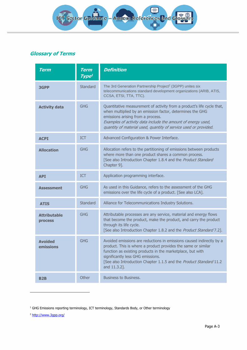
Glossary of Terms
Term Term
Type1
Definition
3GPP Standard The 3rd Generation Partnership Project2 (3GPP) unites six
telecommunications standard development organizations (ARIB, ATIS,
CCSA, ETSI, TTA, TTC).
Activity data GHG Quantitative measurement of activity from a product’s life cycle that,
when multiplied by an emission factor, determines the GHG
emissions arising from a process.
Examples of activity data include the amount of energy used,
quantity of material used, quantity of service used or provided.
ACPI ICT Advanced Configuration & Power Interface.
Allocation GHG Allocation refers to the partitioning of emissions between products
where more than one product shares a common process.
[See also Introduction Chapter 1.8.4 and the Product Standard
Chapter 9].
API ICT Application programming interface.
Assessment GHG As used in this Guidance, refers to the assessment of the GHG
emissions over the life cycle of a product. [See also LCA].
ATIS Standard Alliance for Telecommunications Industry Solutions.
Attributable
process
GHG Attributable processes are any service, material and energy flows
that become the product, make the product, and carry the product
through its life cycle.
[See also Introduction Chapter 1.8.2 and the Product Standard 7.2].
Avoided
emissions
GHG Avoided emissions are reductions in emissions caused indirectly by a
product. This is where a product provides the same or similar
function as existing products in the marketplace, but with
significantly less GHG emissions.
[See also Introduction Chapter 1.1.5 and the Product Standard 11.2
and 11.3.2].
B2B Other Business to Business.
1 GHG Emissions reporting terminology, ICT terminology, Standards Body, or Other terminology
2 http://www.3gpp.org/

Page A-4
Term Term
Type1
Definition
B2C Other Business to Consumer.
BSI Standard British Standards Institution.
CAPEX Other Capital Expenditure.
Cloud ICT Cloud computing is a model for enabling ubiquitous, convenient, on-
demand network access to a shared pool of configurable computing
resources (e.g. networks, servers, storage, applications, and
services) that can be rapidly provisioned and released with minimal
management effort or service provider interaction3.
CO2e GHG Carbon dioxide equivalent. This is the unit of measure used for
comparing the radiative forcing of a GHG to carbon dioxide.
[See also GWP].
Colo
(Colocation Data
Center)
ICT A colocation data center is an independently owned and run building
where multiple data or telecommunications carriers locate their
connections next to one another, enabling customers in the building
to interconnect to them with a minimum of cost and complexity4.
CPE ICT Customer Premises Equipment (also known as Customer Domain
Equipment).
CPU ICT Central Processing Unit.
CRAC ICT Computer Room Air Conditioning.
DEFRA Other UK Government Department for Environment Food and Rural Affairs.
DHCP ICT Dynamic Host Configuration Protocol (DHCP) is a network protocol.
DMS ICT Desktop Managed Services.
(Services provided by specialist ICT companies to businesses to
manage their desktop environments (such as PCs, laptops, tablets
and smartphones).
[see DMS Chapter 3.2]
DNS ICT Domain Name System.
3 NIST Special Publication 800-145 The NIST Definition of Cloud Computing September 2011
4 http://www.city-lifeline.co.uk/page/footer-pages/spelling

Page A-5
Term Term
Type1
Definition
DSLAM ICT Digital subscriber line access multiplexer. (DSLAM is a network
device, which connects multiple customer digital subscriber line
(DSL) interfaces to a high-speed digital communications channel
using multiplexing techniques).
EEIO GHG Environmentally extended input-output. EEIO models estimate GHG
emissions for different product sectors, by allocating national GHG
emissions to groups of products based on economic flows.
[see Box 8.2 in the Product Standard]
Embodied
emissions
GHG The term “embodied emissions” used in this guidance combines the
emissions due to the following life cycle stages: raw material
acquisition and preprocessing, production, distribution and transport,
installation and end-of-life treatment (i.e. all life cycle stages other
than the use stage).
[See also Introduction Chapter 1.7.2].
Emission GHG Releases to air and discharges to water and land that result in GHGs
entering the atmosphere.
Emission factor GHG Amount of greenhouse gases emitted, relative to a unit of activity.
Enabling effect GHG /
ICT
An “enabling effect” is the opportunity an ICT solution has to avoid
GHG emissions in other sectors, which can be attributed back to the
ICT solution as the prime cause of that avoidance.
[See also ‘avoided emissions’].
ERP ICT Enterprise Resource Planning.
ETSI Standard European Telecommunications Standards Institute.
FTE Other Full Time Equivalent.
Functional unit GHG The functional unit is the quantified performance of the product
being assessed, and is used as the reference unit against which the
product is measured.
[See also Introduction Chapter 1.8.1 and the Product Standard
6.3.2].
GHG GHG Greenhouse gas.
GHG emission GHG Release of GHGs to the atmosphere.

Page A-6
Term Term
Type1
Definition
GWP GHG Global Warming Potential. GWP is a factor describing the radiative
forcing impact of one kg of a given greenhouse gas relative to a kg
of carbon dioxide over a given period of time.
[See also Introduction Chapter 1.8.6 and the Product Standard 11.2
and 11.3.1].
HVAC ICT Heating, ventilation, and air conditioning.
I/O or IO ICT Input Output.
IC ICT Integrated Circuit.
ICT ICT Information and Communication Technology.
This guidance document follows the OECD definition5, which has the
following guiding principle:
“ICT products must primarily be intended to fulfill or enable the
function of information processing and communication by electronic
means, including transmission and display.”
[see also the Introduction Chapter 1.1]
IEC Standard International Electrotechnical Commission.
IEEE Standard Institute of Electrical and Electronics Engineers.
IH ICT ICT Hardware.
IMAC ICT “Installs, Moves, Adds and Changes” – term related to activities of
maintenance engineers supporting DMS.
iNEMI ICT International Electronics Manufacturing Initiative.
Inventory
Results
GHG The GHG impact of the studied product per unit of analysis.
[See also Introduction Chapter 1.8.6 and the Product Standard
chapter 11].
IP ICT Internet Protocol.
ISO Standard International Organization for Standardization.
IT ICT Information Technology.
5 OECD: INFORMATION ECONOMY PRODUCT DEFINITIONS BASED ON THE CENTRAL PRODUCT CLASSIFICATION (VERSION
2), DSTI/ICCP/IIS(2008)1/FINAL

Page A-7
Term Term
Type1
Definition
ITU Standard International Telecommunication Union.
LAN ICT Local Area Network.
LCD ICT Liquid Crystal Display.
LCI GHG Life Cycle Inventory.
LCIA GHG Life Cycle Inventory Assessment.
Life cycle GHG Consecutive and interlinked stages of a product system, from raw
material acquisition or generation of natural resources to end-of-life.
Life cycle
assessment
(LCA)
GHG Compilation and evaluation of inputs, outputs and potential
environmental impacts of a product system throughout its lifecycle.
Materiality GHG Materiality is the condition when individual or aggregate errors,
omissions, and misrepresentations have a significant impact on the
GHG inventory results and could influence a user’s decisions.
[See the Product Standard 12.3.3]
MME ICT Maximum Measured Electricity.
MPLS ICT Multi Protocol Label Switching. (A protocol in telecommunications
networks that directs data from one network node to the next).
Network ICT A telecommunications network is a series of points or nodes
interconnected by communication paths6. Networks allow the
transfer of data and sharing of computing resources through groups
of interconnected computers and peripherals.
NIST Standard National Institute of Standards and Technology.
Non-attributable
process
GHG Processes and services, materials and energy flows are not directly
connected to the studied product because they do not become the
product, make the product, or directly carry the product through its
life cycle.
[See also Introduction Chapter 1.8.2 and the Product Standard 7.2].
6 This definition is from http://searchnetworking.techtarget.com. Other definitions of networks include “Any thing reticulated or
decussated, at equal distances, with interstices between the intersections” (Dr. Samuel Johnson, author of the 1755 Dictionary and owner of Hodge).

Page A-8
Term Term
Type1
Definition
OEM ICT Original Equipment Manufacturer.
OS ICT Operating System.
PAIA project ICT Product Attribute to Impact Algorithm, project run by the
Massachusetts Institute of Technology (MIT).
PDU ICT Power Distribution Unit.
Primary data GHG Data from specific processes in the studied product’s life cycle.
Product GHG A product is defined as “any good or service”.
This Guidance includes both “networks” and “software” in the
definition of products, as ICT services.
Proxy data GHG Data from a similar activity that is used as a stand-in for the given
activity. Proxy data can be extrapolated, scaled up, or customized to
represent the given activity.
PUE ICT Power Usage Effectiveness.
PUE7 is a metric which represents the ratio between the total facility
power and the IT equipment power of a data center.
PWB ICT Printed Wiring Board (also referred to as Printed Circuit Board).
RPP ICT Remote Power Panel.
Screening
Assessment
GHG A screening assessment is an initial assessment of a product to
understand what the significant and relevant sources of emissions
are.
[See also Introduction Chapter 1.7.3 and the Product Standard
section 8.3.3].
Secondary data GHG Data that is not from specific processes in the studied product’s life
cycle.
Significance GHG Significance is defined in the Product Standard (box 7.3) as the size
of emissions, removals or GHG intensity.
[See also Introduction Chapter 1.7.4].
7 The Power Usage Effectiveness (PUE) ratio was developed as a key data center efficiency metric by The Green Grid consortium
http://www.thegreengrid.org/
http://www.thegreengrid.org/Global/Content/white-papers/The-Green-Grid-Data-Center-Power-Efficiency-Metrics-PUE-and-DCiE

Page A-9
Term Term
Type1
Definition
SLA ICT Service Level Agreement.
SNMP ICT Simple Network Management Protocol.
SPC ICT Storage Performance Council.
SPEC Standard Standard Performance Evaluation Corporation.
TNS ICT Telecommunications Network Services.
TPC ICT Transaction Processing Performance Council.
TPCF ICT Typical Power Consumption Factor.
Uncertainty GHG Uncertainty refers to the range of values for a specific parameter, or
more generally to the lack of certainty in data or methodology such
as incomplete data, or non-representative factors.
The term uncertainty assessment refers to a systematic procedure to
quantify or qualify the uncertainty in a product inventory.
[See also Introduction Chapter 1.8.5 and the Product Standard
chapter 10].
UPS ICT Uninterruptable Power Supply.
VM ICT Virtual Machine.
VMM ICT Virtual Machine Manager.
VoD ICT Video on Demand.
WAN ICT Wide Area Network.

Page K-1
Acknowledgements1
Steering Committee
Tom Okrasinski, Alcatel Lucent
Gabrielle Ginér, BT
Andie Stephens, Carbon Trust
Michelle Cox, CDP
Darrel Stickler, Cisco
Andreas Kroehling, Deutsche Telekom
Jens Malmodin, Ericsson
Kevin Houston, European Commission (representative)
Andy Lewis, Fujitsu
Simon Mingay, Gartner
Alice Valvodova, Global e-Sustainability Initiative
Chiara Venturini, Global e-Sustainability Initiative
Chris Librie, HP
Jean-Manuel Canet, International Telecommunication Union (ITU-T Study Group 5)
Elsa Olivetti, Massachusetts Institute of Technology
Andrea Brown, World Business Council for Sustainable Development
Mark Didden, World Business Council for Sustainable Development
Cynthia Cummis, World Resources Institute
Andrew Armstrong, WSP
Chapter Leads
Introduction Chapter:
Andie Stephens
Telecommunications Network Services Chapter:
Tom Okrasinski and Glyn Stacey
Desktop Managed Services Chapter:
Andy Lewis
Cloud and Data Center Services Chapter:
Andrew Armstrong and Amaya Souarez
Hardware Chapter:
Tom Okrasinski and Elsa Olivetti
Software Chapter:
Dan Williams
Transport Substitution Chapter:
Darrel Stickler
1 Note that designations are those of the organization the individual worked for at the start of their engagement with the development of the ICT Sector Guidance. Inevitably, people have since changed organizations, and in some cases the organizations themselves have changed.

Page K-2
Technical Working Group
Dan Kilper, Alcatel Lucent
Jaime Llorca, Alcatel Lucent
Tom Okrasinski, Alcatel Lucent
Bill Schaeffer, Alcatel Lucent
Tiffany Finley, BSR
Gabrielle Ginér, BT
Graham Seabrook, BT
Mark Shackleton, BT
Glyn Stacey, BT
Chris Weber, Canadian Standards Association
Doug Farquhar, Capgemini
Jonathan Tapp, Capgemini
Kevin Houston, Carbon Masters
Andie Stephens, Carbon Trust
Hugh Barrass, Cisco
John Malian, Cisco
Rodolfo Milito, Cisco
Darrel Stickler, Cisco
Bob Crooks, Defra
Martin Haeussler, Deutsche Telekom
Andreas Kroehling, Deutsche Telekom
Peter Unger, Deutsche Telekom
Michael Zalan, Deutsche Telekom
Roel Castelein, EMC
Katie Schindall, EMC
Mark Stephan, EMC
Deanna Trudeau, EMC
Simon Redding, Environment Agency
Pernilla Bergmark, Ericsson
Matilda Gustafsson, Ericsson
Jens Malmodin, Ericsson
Andy Lewis, Fujitsu
Mel Melis, Fujitsu
David Fuqua, HP
Jay Keyse, HP
Scott Nyulassy, HP
Saleem Van Groenou, HP
Suzanne Greene, Massachusetts Institute of
Technology
Elsa Olivetti, Massachusetts Institute of
Technology
Hrishi Ballal, Microsoft
Tim Calland, Microsoft
Amaya Souarez, Microsoft
Don Goddard, NetApp
Peter Perrault, NetApp
John Wallerich, NetApp
Jeremy Lardeau, Pricewaterhouse Coopers
Christine Dawes, Telstra
Andrew Ely, Telstra
Garry Nicholls, Telstra
Andy Lawrence, The 451 Group
Christophe Garnier, The Green Grid
Dan Schien, University of Bristol
Rod Tucker, University of Melbourne
Dan Williams, University of Reading
Andrea Brown, World Business Council for
Sustainable Development
Mark Didden, World Business Council for
Sustainable Development
Ben Buckley, World Resources Institute
Laura Draucker, World Resources Institute
Andrew Armstrong, WSP
Carbon Trust Team
Martin Barrow
Will Griffiths
Marta Iglesias
Andie Stephens
Paul Swift
Thanks to the following organizations that provided financial support for the development of this sector
guidance: Alcatel Lucent, BT, Capgemini, Cisco, Deutsche Telekom, EMC, Ericsson, Fujitsu, HP, Microsoft,
NetApp, Telstra.


ICT Sector Guidance built on the
GHG Protocol Product Life Cycle Accounting and Reporting Standard
Chapter 2: Guide for assessing GHG emissions of
Telecommunications Network Services
July 2017
This Guidance has been reviewed for conformance with the GHG Protocol Product Standard.

Page 2-2
Contents
Chapter 2: Guide for assessing GHG emissions of Telecommunications Network Services ...................... 2-1 Executive summary: Telecommunications network services ............................................................. 2-4 2.1 Introduction ..................................................................................................................... 2-5
2.1.1 What is in this chapter ................................................................................................... 2-5 2.1.2 How to use this guidance ............................................................................................... 2-5 2.1.3 The audience for this chapter ......................................................................................... 2-6 2.1.4 Examples: When to use and when not to use this chapter ................................................ 2-6
2.2 Rationale for providing sector guidance for TNS .................................................................. 2-7 2.3 Establishing the scope of a TNS GHG inventory ................................................................... 2-7
2.3.1 Defining the functional unit ............................................................................................ 2-7 2.4 Boundary setting ............................................................................................................... 2-9
2.4.1 Defining TNS life cycle stages and elements .................................................................... 2-9 2.5 Screening ....................................................................................................................... 2-12 2.6 Collecting data and assessing data quality ........................................................................ 2-14 2.7 Allocation ....................................................................................................................... 2-15 2.8 Customer domain ............................................................................................................ 2-16
2.8.1 Customer domain overview .......................................................................................... 2-16 2.8.2 Calculating GHG emissions for the customer domain use stage ....................................... 2-16 2.8.3 Allocation of customer domain use-stage emissions ....................................................... 2-21 2.8.4 Calculating GHG emissions for the customer domain embodied activities ......................... 2-23
2.9 Service platform .............................................................................................................. 2-24 2.9.1 Service platform overview ............................................................................................ 2-24 2.9.2 Calculating GHG emissions for the service platform use stage ......................................... 2-24 2.9.3 Calculating GHG emissions for the service platform embodied activities ........................... 2-33
2.10 Operational activities ....................................................................................................... 2-34 2.10.1 Operational activities overview ..................................................................................... 2-34 2.10.2 Calculating GHG emissions for the operational activities use stage .................................. 2-34 2.10.3 Calculating GHG emissions for the operational activities embodied activities .................... 2-35
Appendix 2.1: TNS case study: Multiprotocol Label Switching (MPLS) service .................................. 2-36 A2.1.1 Customer domain ......................................................................................................... 2-38 A2.1.2 Service platform ........................................................................................................... 2-47 A2.1.3 Operational activities .................................................................................................... 2-52 A2.1.4 Summary ..................................................................................................................... 2-53 A2.1.5 Remarks ...................................................................................................................... 2-54

Page 2-3
Tables
Table 2.1. Examples of descriptions of TNS with appropriate functional units ...................................... 2-8
Table 2.2. TNS main elements and boundary descriptions ................................................................. 2-9
Table 2.3. Scenarios requiring use of primary or secondary data ...................................................... 2-14
Table 2.4. Examples of Typical Power Consumption Factors and PUE factors for
Customer Domain facility types ...................................................................................... 2-17
Table 2.5. Calculating use-stage emissions from customer domain equipment
by means of secondary data: Steps 1 and 2 ................................................................... 2-19
Table 2.6. Calculating use-stage emissions from customer domain equipment
by means of secondary data: Steps 3 to 5 ..................................................................... 2-20
Table 2.7. Network types and associated equipment examples, video-on-demand and mobile data .... 2-31
Table A2.8. Customer domain equipment: Projected router volume requirements for MPLS service .... 2-39
Table A2.9. Customer premises equipment (CPE)/access hardware rules .......................................... 2-40
Table A2.10. Customer domain equipment: Deployed routers (customer data centers – on- ramps) .. 2-41
Table A2.11. Customer domain equipment: Deployed LAN switch equipment (customer data center) . 2-42
Table A2.12. Calculating total embodied emissions of the network using the economic data method .. 2-43
Table A2.13. Examples of TNS equipment life cycle stage guidance ................................................. 2-44
Table A2.14. Average Customer Premises Equipment (CPE) projection ............................................. 2-46
Table A2.15. Calculating use-stage energy consumption for the global MPLS core network ................ 2-48
Table A2.16. Calculating use-stage emissions for the global MPLS core network................................ 2-49
Table A2.17. Calculating use-stage emissions for the global transport platforms carrying MPLS traffic 2-50
Table A2.18. MPLS Service GHG summary and inventory by life cycle stages and TNS elements ......... 2-53
Figures
Figure 2.1. Grouped life cycle stages for the three elements of TNS ................................................. 2-12
Figure 2.2. Router in shared services ............................................................................................. 2-22
Figure 2.3. Decision tree for service platform use-stage GHG emissions calculation methods .............. 2-26
Figure 2.4. End-to-end services using networks from multiple providers ........................................... 2-28
Figure A2.5. The boundary for the MPLS network service being studied ........................................... 2-37
Figure A2.6. GHG emissions calculated for the MPLS service ............................................................ 2-54

Page 2-4
Executive summary: Telecommunications network services
Telecommunications network services (TNS) are provided by specialist information and communication
technology (ICT) companies to both businesses and consumers, they allow the transfer of data and the
sharing of computing resources. TNS can include dedicated private networks or public networks and
include voice and data services. Networks cover a range of types and technologies including: local area
network (LAN) and wide area network (WAN), fixed and mobile networks, satellite and submarine
networks, and the network core. Telecommunications networks were responsible for approximately 22
percent of the total ICT greenhouse gas (GHG) footprint in 2011,1 and no modern ICT system can operate
without them. This chapter provides overall guidance to calculate the greenhouse gas emissions related to
TNS.
TNS are complex in nature, often covering a wide geographical area (e.g., an entire country, or even a
global network), and may include thousands (and in some cases, hundreds of thousands) of items of ICT
equipment. This chapter provides a structure for assessing such complex systems by subdividing TNS into
three distinct elements:
Customer domain — equipment that is part of the TNS, deployed at the end user’s premises
Service platform — network equipment and infrastructure used by the service provider to deliver
the TNS
Operational activities — activities related to the development, deployment, and maintenance of
the TNS.
This chapter provides guidance and calculation methods for assessing each of these elements. The
methods require different levels of detail for assessing the emissions of the life cycle stages depending on
the goals of the assessment, the completeness of information, and the balancing of any trade-offs between
the GHG accounting and reporting principles.
For large and complex TNS it may be difficult to directly measure accurate and detailed primary data,
hence this chapter also provides modeling and calculation methods. It is further recognized that in the
future, network equipment will commonly have the capability to automatically monitor the energy
consumed by a specific network service. Thus the methods provided for the service platform element
include detailed approaches that can incorporate this data as it becomes more available.
Appendix 2.1 to this chapter includes a worked example: a detailed GHG assessment of a global
Multiprotocol Label Switching (MPLS) service
1 The Boston Consulting Group (BCG), “SMARTer 2020: The Role of ICT in Driving a Sustainable Future,” Global e-Sustainability
Initiative (GeSI), 2012, available at http://gesi.org/SMARTer2020

Page 2-5
2.1 Introduction
2.1.1 What is in this chapter This chapter forms part of the ICT Sector Guidance, built on the Greenhouse Gas Protocol Product
Life Cycle Accounting and Reporting Standard (Product Standard) and covers telecommunications
network services (TNS).
This chapter provides guidance and accounting methods for the calculation of GHG emissions
related to TNS.
A telecommunications network is a series of points or nodes interconnected by communication
paths.2 Networks allow the transfer of data and sharing of computing resources through groups
of interconnected computers and peripherals. They are necessary for any ICT system to operate.
A telecommunications network service is a specified set of information/data-transfer capabilities
provided to a group of users via a telecommunications network, and is typically offered through a
service provider.
The chapter provides guidance on the following key items:
Establishing the scope of TNS
Defining the functional unit
Boundary setting (including defining TNS life cycle stages and elements)
Allocation
Calculating inventory results and GHG emissions
This chapter provides a GHG emissions calculation methodology based on dividing the TNS into
three distinct segments (or elements). The assessment of each of these elements is described in
separate sections of the chapter as follows:
Customer domain — equipment that is part of the TNS, deployed at the end user’s
premises;
Service platform — network equipment and infrastructure used by the service provider to
deliver the TNS; and
Operational activities — activities related to the development, deployment, and maintenance
of the TNS.
For each element, use-stage emissions and embodied emissions are calculated. The term
embodied emissions is employed in this chapter to represent the collective emissions from the
following life cycle stages: material acquisition and preprocessing; production; distribution and
storage; and end-of-life.3
The chapter includes a detailed worked example for a global MPLS service in Appendix 2.1.
2.1.2 How to use this guidance
The purpose of this Sector Guidance is to provide additional guidance to practitioners who are
implementing the Product Standard for ICT products (including ICT services). This Sector Guidance follows
a life cycle approach to the assessment of ICT products (including services). The ICT Sector Guidance is a
supplement to the Product Standard, and thus assumes that the reader is familiar with the principles and
content of the Product Standard. The ICT Sector Guidance is divided into chapters, with general guidance
2 http://searchnetworking.techtarget.com.
3 TNS emissions produced from these life cycle stages are treated in this chapter as a collective entity for ease of discussion and calculation — though the practitioner should still account for the emissions from each stage per the principle of completeness.

Page 2-6
provided in the Introduction Chapter, and specific guidance in each of the subject chapters. The chapters
cover the following subjects: Telecommunications Network Services; Desktop Managed Services; Cloud and
Data Center Services; Hardware; and Software.
This chapter should be used in conjunction with the Introduction Chapter and with the Product Standard.
2.1.3 The audience for this chapter
There are several potential users of this chapter:
Suppliers of TNS, who require standard terminology, guidance, and accounting methods to
calculate the GHG emissions of the TNS that they provide. This chapter is intended for TNS
providers who want to calculate the energy and GHG emissions impact of their services to both
better understand where energy is used in the network and to be able to provide information to
their customers
Note: this chapter has been written primarily from a service provider perspective, but is also
applicable to companies and practitioners assessing TNS provided by an internal function or by
an external provider to help establish strategic priorities for GHG reduction actions.
Customers or end users of TNS, who want to understand the GHG emissions of the ICT
products and services in terms of the direct impact of the customer’s equipment as well as the
indirect impact of the TNS provider’s network equipment
Life cycle practitioners, who are assessing the GHG emissions associated with current or
future TNS applications
Consultants, who are tasked with calculating the GHG emissions of TNS on behalf of their
clients
Nongovernmental organizations (NGOs) and advocacy groups, who are addressing the
impact of ICT on climate change, and need a consistent approach to calculating the GHG impact
from TNS
Policymakers, who need a consistent approach to calculating the GHG impact from TNS, to
understand TNS in the context of the wider impact of ICT.
2.1.4 Examples: When to use and when not to use this chapter
Some examples of where this accounting method for TNS should be used:
TNS provider(s) assessing an existing network that they operate, to understand and reduce the
energy use and GHG emissions of the network
TNS provider(s) assessing a planned new network or network service, that is, to obtain a
forward-looking analysis of potential future GHG emissions from the roll out of projected or
expected TNS requirements
Assessing a specific network service for a specific customer; for example, as part of a bid or in
response to a customer request. For example, a service provider’s customer may be asking for
the GHG emissions associated with the delivery of a Multiprotocol Label Switching (MPLS)
network service. In this instance, it is likely that the assessment would be performed by the
provider of the service.
Assessing a service being provided across multiple networks (from multiple providers) – for
example, supply of a telepresence service. The assessment is likely to be performed by the
telepresence equipment supplier or by the telecommunications service provider. In this case, the
service is likely to be using multiple networks from multiple network providers and a mix of
different network types such as a mobile network, fixed-line network, and the internet.
Assessing a service provided across a single provider’s network – for example, assessment of an
average one-minute telephone call over the service provider’s network.

Page 2-7
This accounting method for TNS should not be used for the following:
Comparative product assessments among different TNS where the results will be used to
demonstrate a competitive or marketing advantage.
2.2 Rationale for providing sector guidance for TNS TNS are different from other services. Typically TNS use multiple shared and dedicated resources. Hence
the major difference between the GHG emissions of TNS and a non-ICT service is that the emissions of a
particular piece of TNS equipment need to be allocated and aggregated in order to calculate the emissions
associated with a particular TNS. In addition, there are typically numerous ways that a TNS provider can
deliver a service, or even an instance of a service. This chapter focuses on these differences and the
calculation methods that can be employed to assess the GHG emissions more easily. Furthermore, the
methods detailed in this chapter are set up to address the complexities of TNS equipment and networks as
well as the rapid evolution of new technologies and network transformation.
2.3 Establishing the scope of a TNS GHG inventory
2.3.1 Defining the functional unit
In defining the TNS functional unit, it is important to first establish the scope of the particular service being
assessed. Then the functional unit should clearly state the magnitude of the service’s duty or deliverables,
the duration of the service’s life, and the expected level of service quality and reliability. Table 2.1 provides
some examples of TNS functional units.

Page 2-8
Table 2.1. Examples of descriptions of TNS with appropriate functional units
Service
(examples)
Description of functional unit (examples)
Magnitude Duration Quality
Phone call using a
telecommunications
network
Voice call over a single
carrier’s network
One-minute
phone call
Listening – e.g., narrow
/ wideband mean
opinion score (MOS)
limits
Conversational – e.g.,
echo / latency limits
Transmission – ITU E-
model rating limit
Data transfer using a
telecommunications
network
Transfer of 1 megabyte
(MB) of data
Packet-switched data
over a single carrier’s
network
Extent of
time
necessary to
transfer 1
MB of data
Physical layer net bit
rate –10 megabits per
second (Mbps)
Includes data link and
higher layer overhead
Multi-protocol label
switching (MPLS)
service
Single customer service
Total network ports –
10,000
Capacity – 1 Mbps
Geographical spread of
end users – 60 specified
countries
Length of
service
contract –
delivery of
MPLS service
to a
customer for
3 years
Internet Protocol (IP)
precedence
Committed access rate
Random early detection
Weighted fair queueing
Class / Priority based
queueing
Video on demand
(VoD) service
Single customer service
VoD mean customer
traffic – 1 Mbps
VoD network traffic
capacity – 10 Mbps
Geographical spread of
end users (mean distance
from customer to network
core4) - 50 km
Single service provider’s
network
Length of
service
contract –
delivery of
VoD service
to a
customer for
1 year
Client quality of service
(QoS) specification
Initial latency
Scheduling
Jitter
Throughput
4 Network core is the central area of a telecommunications network where large-scale switching, routing, data storage and
long-haul transmission transactions occur.

Page 2-9
2.4 Boundary setting
2.4.1 Defining TNS life cycle stages and elements
TNS are provided by specialist ICT companies to both businesses and consumers. They allow the transfer
of data and the sharing of computing resources. TNS can include dedicated private networks or public
networks and include voice and data services. Networks cover a range of types and technologies including:
local area network (LAN) and wide area network (WAN), fixed and mobile networks, satellite and
submarine networks, and the network core. To provide a clear framework for the assessment, and to more
easily define the boundary, the methodology recommended in this chapter subdivides TNS into three
elements:
Customer domain
Service platform
Operational activities
These elements are a convenient means for grouping distinct parts of the TNS. Each element has its own
boundary definition, and the elements are commonly understood by providers of TNS. Each element
includes the equipment (hardware and software) and the life cycle processes related to that element.
Because each element is very different in scope, it is necessary to use different calculation methods for
each element (these methods are described in detail later in the chapter). The elements and their
boundary descriptions are shown in Table 2.2.
Table 2.2. TNS main elements and boundary descriptions
Element Boundary description
Customer
domain
TNS equipment deployed at the end user’s premises
Attributable processes:
All ICT equipment (e.g., routers, PCs, videoconferencing systems,
switches, servers, telephones) and related support equipment (e.g.,
cabling, racking) that is required to provide the TNS deployed in the
customer domain – also known as customer premises equipment (CPE).
This equipment may be owned by either the customer or the TNS
provider
Cooling and uninterruptable power supply equipment (where necessary)
supporting the ICT equipment that provides the TNS over its lifetime
End-user equipment such as PCs, video conferencing systems, and
telephones that are part of the service being provided (either included
by the service provider or owned by the customer)
Note: It is necessary to clearly document whether end-user equipment is
included within the scope of the assessment, particularly if this is being
carried out alongside a desktop managed services study to avoid the
possibility of double counting.
Non-attributable processes:
Electricity and other energy related emissions from residences, facilities,
or general offices of the service provider’s customers (end users)

Page 2-10
Element Boundary description
Service
platform
Network equipment and infrastructure used by the service provider to
deliver the TNS
Attributable processes:
All ICT equipment (e.g., switches, routers, transport layers) and support
equipment (e.g., cabling, racking, antennae) used by the TNS provider
in delivering the service being assessed
Ancillary support equipment such as heating, ventilation, and air
conditioning (HVAC)
Uninterruptable power supply (UPS) equipment that is calculated
separately rather than using a cooling power usage effectiveness (PUE)
factor (see Section 2.8 “Customer domain,” for an explanation of PUE
factors)
Note: This includes all electricity consumption within central offices and
data centers
Electricity and other HVAC energy-related emissions associated with
network equipment and infrastructure that are provided as part of the
TNS by the service provider
Non-attributable processes:
Upstream emissions from other capital equipment, that is, those
emissions produced from the manufacturing of such capital equipment;
for example, corporate facilities, ICT equipment, and ancillary support
equipment such as general office, lighting, and HVAC equipment not
directly part of the service platform
Note: Emissions from capital equipment used in the upstream stages, for
example, suppliers’ buildings, plant, and machinery will be generally
included in emissions assessment calculations made where financial
economic input-output data is used

Page 2-11
Element Boundary description
Operational
activities
Activities related to the development, deployment, and maintenance of
the TNS
Attributable processes:
People (labor)-related activities directly linked to the service being
assessed including solution design, surveying, planning deployment /
installation, maintenance, and technical support over the service’s
lifetime
Dedicated nontechnical support such as product management, sales, and
marketing
Activities associated with decommissioning of ICT equipment
Note: Embodied emissions may be excluded from the GHG inventory for
operational activities if it is determined through appropriate screening
methods or past analysis / findings that the impact is of low significance5
Non-attributable processes:
People related activities not directly linked to the service being assessed,
that is, activities that are supporting other activities or different services,
which are not the subject of the current assessment
Staff traveling to their normal place of work (i.e., commuting)
Upstream emissions from capital goods (e.g., construction of buildings,
machinery)
5 Refer to the Introduction Chapter for further discussion of significance.

Page 2-12
Figure 2.1 maps the life cycle processes associated with each of the three elements comprising TNS. It also
shows how these life cycle processes have been further grouped into use and embodied GHG emissions for
ease of calculation in this ICT Sector Guidance.
Figure 2.1. Grouped life cycle stages for the three elements of TNS
2.5 Screening
Screening is described in detail in chapter 8 of the Product Standard and in the Introduction Chapter of this
ICT Sector Guidance. The business goals, as well as the screening step, will enable companies to prioritize
the collection of primary and secondary data on the processes and process inputs that have significant
impact on the inventory results. Note that the Product Standard requires that primary data be collected for
all processes under the ownership or control of the reporting company. For example, if a TNS provider is
carrying out the assessment, it is required to use primary data to calculate emissions from the use stage of
the equipment in the service platform that is under the TNS provider’s control.

Page 2-13
Example: Use-stage screening estimate for TNS – video on demand (VoD)
In this example, the GHG emissions are calculated for delivery of a VoD service to a customer. The
customer equipment includes a GPON (gigabit passive optical network) fiber to the home optical
network unit, a home gateway, a digital video box, and a television. These customer premises
devices are likely to consume in the order of ~100 watts (W), whereas the total service platform
contribution (allocated by proportion of traffic) might be as small as 1 watt. Therefore, a detailed
assessment of the service platform emissions is unlikely to significantly impact the inventory results.
This example demonstrates the method for conducting the top-down6 calculation and using that
result to screen for whether the service platform contribution is significant. The values shown here
are illustrative and may not reflect a case in practice.
Example values
Customer domain equipment:
Entertainment system: 600W, (8-hour use) 5 kilowatt hours per day (kWh/day)
Digital video box: 30W, (8-hour use) 0.2 kWh/day
Home gateway: 15W, (24-hour use) 0.4 kWh/day
Service platform equipment
Network access equipment:
Optical line termination (OLT): 40 W x 24 hours/day = 1 kWh/day
OLT capacity: 2.5 gigabits per second (Gbps)
OLT mean utilization: 10 percent (time in use)
OLT efficiency: 1.0 kWh/day ÷ (2.5 Gbps × 10%) = 4 kWh/day-Gbps
VoD service:
VoD mean traffic: 1000 Gbps
VoD mean customer traffic: 1.0 megabits per second (Mbps)
VoD capacity: 10 Mbps
Service platform:
Total mean traffic: 10 terabits per second (Tbps)
Total service platform power consumption: 170 megawatt hours per day (MWh/day)
Customers: 1 million
Screening tests:
Screening threshold: 10 percent (of the total power consumption)
Bandwidth weighted approach
Calculating customer domain use-stage energy usage:
ECD (per day) = (5 kWh/day + 0.2 kWh/day + 0.4 kWh/day) x 106 customers = 5,600 MWh/day
Bandwidth fraction (VoD customer traffic / VoD capacity) = 1.0 Mbps / 10 Mbps = 0.1
Screening Test 1: Top-down6 service platform calculation:
EVoD = 170 MWh/day × 0.1 (bandwidth fraction) = 17 MWh/day
6 The top-down approach starts with high level organizational or service platform GHG emissions data and allocates a portion to the service being assessed.

Page 2-14
ECD = 5,600 MWh/day >> EVoD = 17 MWh/day
Therefore, energy use for the VoD service platform equipment is much less (0.3 percent) than the energy
use of the customer domain equipment, and a detailed accounting of the network emissions is unlikely to
significantly impact the assessment.
Screening Test 2: Service platform equipment energy usage versus customer domain equipment energy
usage ratio calculation:
The OLT is expected to be the least efficient network element.
EVoD = 1,000 Gbps × 4 kWh/day-Gbps = 4,000 kWh/day or 4 MWh/day
ECD = 5,600 MWh/day >> EVoD = 4 MWh/day
Therefore, similar to Test 1 the energy usage for the VoD service platform equipment is much less (0.07
percent) than the energy usage of the customer domain equipment, and a detailed accounting of the
network emissions is unlikely to significantly impact the assessment.
If data is available, the preferred screening approach is the one in Screening Test 2, because it is typically
more conservative.
2.6 Collecting data and assessing data quality This section complements Section 1.8.3 of the Introduction Chapter.
Studies of TNS with long operating periods have often shown that the use stage dominates all the other
life cycle stages (see, as an example, Appendix 2.1: TNS case study: Multiprotocol Label Switching (MPLS)
service”). Therefore, it may be acceptable to group all stages other than the use stage together
(collectively referred to as the embodied emissions). This can significantly simplify the analysis while
keeping sufficient accuracy depending on the purpose of the assessment. However, it could result in loss of
overall GHG reduction potential because it may not be transparent as to where savings can occur in the
individual life cycle stages.
The Product Standard requires the reporting entity to collect primary data for activities under its ownership
or control. This requirement will have a different effect depending on who is performing the assessment,
for example, the TNS may involve multiple networks under multiple service provider ownership. Table 2.3
provides guidance on interpreting this requirement for different parts of the TNS, depending on who is
performing the assessment.
Table 2.3. Scenarios requiring use of primary or secondary data
Who is performing the
assessment
(i.e., the reporting entity)
Customer domain
Service platform (network
provided by the service provider)
Service platform (network
provided by a third party provider)
Service provider Secondary data
may be used
Primary data required Secondary data may be used
End-user company Primary data
required
Secondary data may be
used
Secondary data may be
used

Page 2-15
Because of the complex and extensive nature of telecommunications networks, it may not be practical to
collect all required primary data through direct measurement. If this is the case, modeling and calculation
techniques should be used to collect the primary data. Examples include sampling of switch and router
equipment used in the network, and modeling of complex networks using representative equipment.
Modeling and calculation techniques may be especially useful for a TNS case where there is a huge range
of variation in how the TNS are delivered. For example, the same service between identical endpoints may
be delivered using different network paths depending on network load, cost, and other factors. Also
individual data packets may be delivered over different paths.
Where primary data is not required (where processes are not under the ownership or control of the
reporting company), then secondary data, which may be more readily available, may be used to
supplement the primary data.
The customer domain and service platform elements comprise numerous individual pieces of ICT
equipment. The guidance provided in the Hardware Chapter of this ICT Sector Guidance is applicable to
any ICT equipment, so refer to the Hardware Chapter for guidance on the various data collection and
calculation methods available for assessing the life cycle emissions of ICT equipment.
2.7 Allocation A key step in the assessment of TNS is the allocation of emissions from each piece of ICT equipment to the
TNS being studied. This chapter includes allocation methods that can be used for TNS with a level of
quality sufficient to meet the assessment goals.
TNS, like other ICT products and services, includes significant instances in which equipment is shared
among multiple services. As a consequence, GHG emissions associated with some TNS-attributable
processes will need to be allocated among the services using them. The criterion by which allocation
should be made is critical to a consistent approach of the GHG assessment, and hence a key feature of this
chapter.
Allocation may follow, for example:
Usage-based allocation, for example, number of subscribers or amount of data
Provisioned capacity, for example, ports or bandwidth
Mean traffic across a network or equipment
For different network layers, different allocation methods may be appropriate.
See chapter 9 of the Product Standard for detailed guidance on allocation methods and calculations. In
addition, for allocation guidance specific to ICT, refer to International Telecommunication Union,
“Methodology for the Assessment of the Environmental Impact of Information and Communication
Technology Goods, Networks and Services,” section 5.2.3.3, 7 and European Telecommunications
Standards Institute, “Life Cycle Assessment (LCA) of ICT equipment, Networks and Services: General
Methodology and Common Requirements,” section 5.3.3.8
7 International Telecommunication Union (ITU), “Methodology for the Assessment of the Environmental Impact of Information and Communication Technology Goods, Networks and Services,” ITU-T L.1410, ITU, Geneva, 2012, available at
http://handle.itu.int/11.1002/1000/11430. 8 European Telecommunications Standards Institute, “Environmental Engineering (EE); Life Cycle Assessment (LCA) of ICT Equipment, Networks and Services; General Methodology and Common Requirements,” ETSI TS 103 199 V.1.1.1, 2011, available at http://etsi.org/ (Note that this was superseded by ETSI ES 203 199 published in December 2014, which is technically equivalent to the revised ITU-T L.1410 also published in December 2014).

Page 2-16
2.8 Customer domain
2.8.1 Customer domain overview The customer domain is defined as TNS equipment that is deployed at the end user’s premises. Customer
domain equipment can be further divided into:
Equipment that supports a single service, that is, dedicated equipment, such as an IP phone
Equipment that supports multiple services, for example, routers and laptops
In the latter case all relevant GHG emissions should be allocated (see Section 2.8.3 ”Allocation of customer
domain use-stage emissions”).
2.8.2 Calculating GHG emissions for the customer domain use stage
Overview of customer domain use-stage calculation methods
Using primary data
Using primary data to calculate customer domain use-stage emissions will result in the most accurate
inventory results. However, for many reasons, primary data may not be readily available to the entity
performing the GHG assessment. In such cases, secondary data can be used (unless the use-stage
processes are under the ownership or control of the reporting company).
Using secondary data
Secondary data may be estimated from the measured typical power consumption of the customer domain
equipment under normal usage conditions and with a relevant usage profile applied (e.g., hours active,
hours in standby, and hours off per year).
Where only “full load” and “no load” power consumption data is available it may be acceptable to use the
average of these two figures, provided that the underlying assumptions are fully noted and documented in
the GHG emissions assessment. Preferably, a weighted average of multiple use profiles should be used.
Typical power consumption factor (TPCF) and power usage effectiveness (PUE) factor: If only
the maximum rated power consumption is available (as opposed to the measured power consumption
under operating conditions), a TPCF may be applied. For example, a wireless modem may have a
maximum power rating of 20 watts for the design of its electrical circuits and overload protection, but its
more typical power consumption under operating conditions may be 15 watts: thus it would have a TPCF
of 0.75.
In these cases it is important to have knowledge of the type of equipment and its operational aspects to
more properly estimate the TPCF for its intended type of service. Equipment manufacturers may have
estimates of TPCFs for their equipment based on defined operating conditions. In all cases, if a TPCF
approach is selected, then the basis for selecting the factor should be fully noted and documented in the
GHG inventory report. Note that ICT equipment manufacturers can provide equipment usage and user-
profile data that can be used as primary data in the assessment. For example, equipment manufacturers
may provide power consumption in different operational modes and conditions and typical number of hours
per day or per year that the equipment spends in each of the operational modes. This data can be used to

Page 2-17
calculate energy consumption over a period of time. Equipment user profiles or typical power data may
also be available from published reports.
The energy required by any equipment ancillary to the operation of the customer domain equipment, for
example, external cooling, power supply filtering/conversion, uninterruptible power supply (UPS), should
also be taken into account when determining customer domain use-stage emissions. An appropriate
accounting should be made according to the data and information available, and the expertise and
practices of the company undertaking the assessment (e.g., cooling proportioning with the customer
domain equipment). As an alternative, a power usage effectiveness9 (PUE) factor may be applied that
accommodates the power use for such ancillary equipment. The PUE factor can be based on equipment
operating in different facility types, for example, server center or video data storage center. Note that a
value of 1.0 would mean that no additional energy is used by the ancillary equipment. As an illustration,
Table 2.4 shows the hypothetical TPCF and PUE values for a few types of customer domain facilities. For
the server center, a PUE value of 1.6 means that 0.6 watts of power for cooling, power conversion, UPS
losses, and so on are used for every 1 watt consumed by the server equipment itself.
Note: PUE is a common metric used to measure data center efficiency. For more on data centers and PUE,
see the Cloud Computing and Data Center Services Chapter of this ICT Sector Guidance.
Table 2.4. Examples of Typical Power Consumption Factors and PUE factors for Customer Domain facility types
Customer domain facility
type
Hypothetical typical power consumption factor (TPCF)
(typical power consumption as a proportion of maximum
power rating)
Hypothetical power usage effectiveness
factor (PUE)
(total facility power divided by ICT
equipment power)
Server center 0.75 1.6
Video storage
center 0.75 1.5
Switching center 0.75 1.4
Notes
1. The Uptime Institute Data Center survey for 2014 reported the following industry average PUE factors: 1.89 (2011);
1.8 (2012); 1.67 (2013); 1.7 (2014).
https://journal.uptimeinstitute.com/2014-data-center-industry-survey/
2. The techUK CCA report for UK data centers reports an average PUE of 1.87 for 2014.
https://www.techuk.org/images/CCA_First_Target_Report_final.pdf (page 14)
3. Hyperscale Internet Data Centers have much lower PUE factors (often less than 1.1), but these are not typical of
telecommunication network data centers.
4. BT have analyzed a sample of 118 devices used as customer domain equipment, that have a quoted maximum and
typical power consumption – the average TPCF for these is 0.73.
9 Green Grid defines PUE as total facility power divided by the IT equipment power.

Page 2-18
Note: use-stage GHG emissions assessments can employ both primary and secondary data depending on
the availability of each type of data as well as the purpose and goal of the overall assessment. In all cases,
documentation per the Product Standard should be followed so that the basis for the calculations and
results are transparent.
Calculating customer domain use-stage emissions by means of primary data
When calculating the use-stage GHG emissions of customer domain equipment using primary data, the
following data should be collected:
Power or energy10 consumed by individual units of equipment (primary data collected from actual
measurements)
Power or energy consumed by any ancillary equipment (e.g., cooling, power conversion, UPS)
supporting the customer domain equipment
Emission factors for regional or country-specific grid average electricity11 (being averages, these
factors will be secondary data)
The steps below can be followed in order to obtain energy data for the use stage and to assess the
associated GHG emissions.
Step 1: Compile an inventory of all the customer domain equipment deployed (including ancillary
equipment) in delivering the TNS. This information can typically be obtained from the service
provider, the equipment suppliers, and/or the TNS solution design team.
Step 2: Compile the collected data on power or energy consumed per equipment unit, including
any ancillary equipment. If there are any gaps, secondary data should then be used – see section
below for guidance on the collection and use of secondary data.
Step 3: For each type of equipment, calculate the total energy use (e.g., in kilowatt hours (kWh),
megawatt hours (MWh), or gigawatts hours (GWh)) for the period of time being assessed. See
also the Hardware Chapter of this ICT Sector Guidance to calculate use-stage emissions from ICT
equipment.
Step 4: Sum the values from each type of equipment to give the total energy used from the
dedicated equipment together with the allocated values from any shared customer equipment
within the customer domain (see Section 2.7 “Allocation,” and Section 2.8.3 “Allocation of
customer domain use-stage emissions”).
Step 5: Multiply the energy consumption totals by the relevant national or regional electricity grid
average emission factors to calculate total GHG emissions for the use stage of the customer
domain equipment.
Calculating customer domain use-stage emissions by means of secondary data
When calculating the use-stage GHG emissions of customer domain equipment using secondary data, the
practitioner should estimate typical energy consumption of the ICT equipment based on equipment type
10 The determination of whether power or energy data is collected may depend on the measurement methods and type of
measurement equipment employed.
11 These can be obtained from government departments such as Defra in the UK (www.defra.gov.uk), from the International
Energy Agency (www.iea.org/) and from databases that compile different conversion factors for different countries. Where a
particular country conversion factor is not available, regional averages can be used. See Introduction Chapter Section 1.8.6 for
sources of emission factors.

Page 2-19
and anticipated usage profile. The results should then be combined with the relevant country/region
electricity grid average emission factors to provide the total GHG emissions. In practice, the steps outlined
above can be followed with the changes noted for Step 2 below.
Steps 1 and 3 to 5: remain the same as defined above.
Step 2: For each type of equipment, obtain or create typical usage profiles: the amount of time,
(e.g., hours/day, the equipment is in each power state [on mode, idle or standby mode, off or
zero power mode]). If the analysis is forward-looking (e.g., projection of the expected customer
and or contract requirements for the deployment of the service) and could be subject to
variability, the usage profile should consider, as a minimum, two scenarios: a maximum (worst
case) and a minimum (best case) from which either the average (across all stages of operation)
or worst case can be used depending on which is considered most appropriate to the study, with
all assumptions clearly documented. This data will typically be obtained from consultation with
the equipment suppliers and experts with experience in using the equipment in similar setups.
Where there are data gaps, proxy information may be gathered from sources such as studies on
similar equipment, solutions, or projects from internal or external sources. As an alternative,
typical power consumption factors (TPCF) and power usage effectiveness (PUE) factors can be
applied to complete the calculation: see section above on TPCF and PUE factors.
Example: Using secondary data to calculate customer domain use stage
Steps 1 and 2: For the TNS under assessment within the customer domain, a table of equipment
types and their power consumption was created (see Table 2.5). An estimated typical power
consumption factor (TPCF) of 0.75 was applied to scale down from max power ratings in this
example because actual power consumption values (primary data) were not available. It was also
necessary to estimate a power usage effectiveness (PUE) factor of 1.7 and equipment utilization
rates (duty cycle as shown in columns E and F below) to calculate typical energy use per day (stated
in kilowatt hours).
Table 2.5. Calculating use-stage emissions from customer domain equipment by means of secondary data: Steps 1 and 2
Calculation A B C A×C=D E F
(D×E)+
(B×F)=G
H G×H=I
Cu
sto
me
r do
ma
in
eq
uip
me
nt ty
pe
Ma
x p
ow
er (k
W)
Sta
nd
by p
ow
er (k
W)
TP
CF
Typ
ica
l on
po
we
r
(kW
)
Typ
ica
l time
on
(ho
urs
/d
ay)
Sta
nd
by (h
ou
rs/d
ay)
En
erg
y u
se
pe
r da
y
(kW
h)
PU
E fa
cto
r
Typ
ica
l en
erg
y u
se
pe
r da
y (k
Wh
)
Router 0.4 N/A 0.75 0.3 24 N/A 7.2 1.7 12.2
Switch 0.2 N/A 0.8 0.16 24 N/A 3.8 1.7 6.5
HD video
conferencing
unit
1.3 0.3 0.7 0.91 2 22 8.4 1.7 14.3
N/A = Not applicable to this type of TNS equipment currently

Page 2-20
Steps 3 to 5: The customer domain use-stage GHG emissions are then calculated based on the
number of each type of equipment deployed in each country. As shown in Table 2.6, the number of
each type of equipment is multiplied by the typical daily energy use and then multiplied by the
relevant country electricity grid emission factor to give the GHG emissions for the customer domain
equipment use stage. This figure can then be multiplied by the estimated number of days per year
the equipment is in operation to provide the annual GHG emissions (given that one year was the
time period under assessment).
Table 2.6. Calculating use-stage emissions from customer domain equipment by means of secondary data: Steps 3 to 5
Calculation J --
I
(from Table 2.5)
K L J×I×K×L=M
Cu
sto
me
r do
ma
in
eq
uip
me
nt ty
pe
Eq
uip
me
nt
(nu
mb
er o
f un
its)
Co
un
try o
f
insta
llatio
n
En
erg
y u
se
pe
r
da
y
(kW
h)
Co
un
try e
ne
rgy
mix
em
issio
n
facto
r 1
(kg
CO
2 e/k
Wh
)
Da
ys o
f op
era
tion
pe
r ye
ar
An
nu
al e
mis
sio
ns
(kg
CO
2 e)
Router 2 Country A 12.2 0.5826 365 5,190
Switch 10 Country A 6.5 0.5826 365 13,800
Switch 3 Country B 6.5 0.6141 365 4,370
HD video
conferencing
unit
2 Country A 14.3 0.5826 2502 4,170
Total – all customer domain equipment 27,530
Notes
1. Hypothetical country emission factor – see footnote 11 or the Introduction Chapter Section 1.8.6 for recommended
reference sources.
2. Assumed basis: 50 weeks per year and 5 days per week usage.
Calculating customer domain use-stage emissions by means of life cycle stage ratio profiling
When assessing the use-stage GHG emissions of customer domain equipment using life cycle stage ratio
profiling, the practitioner can estimate to a lesser degree of accuracy the use-stage emissions as a
percentage (or ratio) of the total life cycle GHG emissions while accounting for the equipment type, usage
profile, and country/region of use. The percentages or ratio values are developed based on historical life
cycle assessments for different ICT equipment types under certain usage profiles. Note: these life cycle
stage ratio values are highly dependent on the conditions of the applied historical life cycle assessments,
such as the configuration of service, grid emission factors, and equipment operation. Refer to the ICT
Hardware Chapter for a more detailed discussion of life cycle stage ratio profiling. Appendix 2.1 also
provides an example of life cycle ratios for various types of customer domain equipment.

Page 2-21
2.8.3 Allocation of customer domain use-stage emissions
In certain cases, customer domain equipment will be dedicated to the service solution under study.
However, some types of equipment, for example access switches/routers, and certain types of enterprise
equipment, for example, laptops, may be shared by a number of services within the customer domain. A
means of allocating the emissions to each service has to be determined. Services can be allocated on the
basis of:
Proportion of peak bandwidth capacity or mean traffic, or
Number of ports dedicated to the assessed TNS (typically by the network design experts)
Using the peak-capacity or mean-traffic-allocation method, use-stage emissions can be allocated to the
studied TNS based on the proportion of peak capacity or mean traffic provisioned by the TNS. The
allocation calculation can be written as:
Power or energy allocated to TNS = [(Peak bandwidth capacity × Provisioning factor) ÷ Total capacity]
× Total power or energy
Or
Power or energy allocated to TNS = [(Mean traffic allocated to TNS × Provisioning factor) ÷ Total mean
traffic across the entire network] × Total power or energy
In general the energy consumed by a service will have some functional dependence on the mean traffic
that includes service-specific architectural features in the equipment. For example, some services may have
special provisioning requirements that are unique to that service and need to be factored into the
allocation. There may also be multiple TNS provided within the assessment by the service provider. To
account for these mean-traffic variations, the calculation can be written as:
Power or energy allocated to TNS = {[(Mean traffic for TNS Type 1 × Provisioning factor for TNS Type
1) + (Mean traffic for TNS Type 2 × Provisioning factor for TNS Type 2) + (Mean traffic for TNS Type 3
× Provisioning factor for TNS Type 3) + …] ÷ Total mean traffic} × Total power or energy
Provisioning factors are particularly important because equipment is often deployed with capacity that is
significantly higher than the mean-traffic rate and some services have much higher peak capacity
requirements than their mean traffic would indicate. The provisioning factor can account for a wide range
of capacity planning requirements including quality of service, utilization requirements, traffic growth, and
redundancy, (both planned and unplanned12). It also can account for the different network protocols being
adopted such as multi-protocol label switching (MPLS) or asymmetric digital subscriber line (ADSL).
If redundancy is uniformly provisioned across all services using the equipment, then the total redundancy
can be allocated to each of the services in proportion to the service’s share of total mean traffic.
The allocation can take on a variety of different calculation methods to account for the service traffic
dependence on the equipment power. The choice of method should appropriately account for the expected
behavior of the equipment.
12 For example, unplanned redundancy can occur if equipment is left switched on because of a lack of funds for decommissioning. The equipment may have been associated with a service which is no longer provided.

Page 2-22
Note that although the power of an individual component in a network may not have a strong traffic
dependence, the number of components deployed in the network may depend strongly on the mean
traffic, and therefore the mean-traffic approach is preferred in such cases. Including the appropriate
provisioning factors will account for any service-dependent redundancy or performance requirements that
are not reflected in the mean traffic. Traffic fractions involving measured mean quantities are preferred,
but provisioned capacities can be used if the measured values are not available.
Example: Customer domain use-stage allocation based on peak bandwidth capacity
A router is shared between three services with peak bandwidth capacity as follows:
Service a: 400 Mbps
Service b: 150 Mbps
Service c: 20 Mbps
As shown in Figure 2.2, if the 150 Mbps service (b) is selected for assessment, then the proportion
of energy consumption allocated to the assessed service is: 150 Mbps ÷ 570 Mbps, which is 26% of
the total router’s bandwidth.
Figure 2.2. Router in shared services
Notes
1. Alternative factors can be used to allocate power consumption to different services, e.g., mean-traffic
throughput in Mbps, as long as the same factor is used for each service in the allocation process being
undertaken.
2. Some services might use more hardware in the router such as specialized integrated circuits for
security or increased quality of service, and thus might require additional weighting that is dependent
on the router design itself.
If, for example, Service c also uses dedicated hardware in the router that accounts for 20% of the total
power, then the shared service breakdown becomes:
Service a: 421W, Service b: 158W, and Service c: 171W
Service a: 400 Mbps
400Mb Router
(Power: 750 W) Service b: 150 Mbps
400Mb
Service c: 20 Mbps
400Mb
Service a: 526.3 W (70.2%)
Service b: 197.4 W (26.3%)
Service c: 26.3 W (3.5 %)

Page 2-23
2.8.4 Calculating GHG emissions for the customer domain embodied activities
Calculation methods for assessing the embodied GHG emissions (e.g., emissions from the material
acquisition and preprocessing; production; distribution and storage; and end-of-life stages) of customer
domain equipment are covered in detail in the Hardware Chapter. Embodied emissions from the customer
domain equipment may also need to be allocated to the TNS under study depending on how that
equipment shares the service. The allocation procedure can employ the same methods described
previously for the customer domain use-stage emissions.
End-of-life stage considerations:
In practice, end-of-life stage GHG emissions for customer domain equipment tend to be very small relative
to the other stages. If a detailed assessment is necessary or recommended (based on a screening
assessment), then it should include both the planned and unplanned (based on the equipment’s particular
in-field failure rate)13 removal of equipment from service during its operational life, or as the equipment
reaches the end of its contract period, or when the service is ceased. If recycling occurs, the practitioner
should also refer to the Product Standard, which provides two specific methods for allocating emissions
and removals between product life cycles: the closed-loop approximation method and the recycled-content
method.
13 In-field failure rate does not only impact end-of-life treatment but also the production and use of material and will require
additional units of hardware.

Page 2-24
2.9 Service platform
2.9.1 Service platform overview
The service platform refers to all ICT equipment and associated support equipment that directly support
the service: for example, switches, routers, transport layers, cabling, racking and ancillary support
equipment such as cooling, power conditioning, and UPS equipment. The ICT and associated support
equipment is likely to be shared by multiple services. Therefore, as with customer domain equipment, the
emissions from shared service platform equipment should be allocated to the service platform being
assessed. Allocation methods for the service platform equipment are the same as those used for the
customer domain equipment (see Section 2.8.3 “Allocation of customer domain use-stage emissions”).
The service platform tends to be the most complex part of assessing the GHG emissions of TNS because
services may cross multiple provider domains and use diverse paths through a network.
Several methods may be used to calculate emissions from the service platform. These are outlined in the
sections below.
2.9.2 Calculating GHG emissions for the service platform use stage
Overview of calculation methods
Two approaches are described in this section:
Top-down approach: High-level service platform method
Bottom-up approach: Equipment inventory method
In summary, the top-down approach starts with high-level organizational or service platform GHG
emissions data and allocates a portion to the service being assessed. The bottom-up approach assesses
the GHG emissions of each individual piece of equipment involved in the delivery of the service and
allocates a portion of each to the service being assessed, with all equipment portions then being summed
up.
Although the bottom-up approach provides greater accuracy, it may not be reasonable to collect the large
extent of data required (i.e., data collection may require an unpractical amount of resources). Further, the
quality and precision of the GHG emissions assessment may not justify a bottom-up approach. For these
reasons, a top-down approach may be a more practical choice given the level of detail available or the
relative size and complexity of the TNS being assessed.
The top-down approach may overestimate the GHG emissions associated with TNS for newer services
because most networks support multiple services and include legacy equipment associated with less
efficient, low bandwidth services. In other words, the emissions assessment of the more efficient services
may be overestimated and the emissions of less efficient services may be underestimated.
To determine the level of analysis required, a screening assessment of the TNS should be carried out.
Screening is discussed in Section 2.5 “Screening” of this chapter, as well as in the Introduction Chapter of
this ICT Sector Guidance and chapter 8 of the Product Standard.

Page 2-25
In the bottom-up equipment inventory method, the total power consumption and hence the GHG emissions
impact of a service platform can be calculated by analyzing the equipment employed within the platform
(similar to the steps detailed in the customer domain use stage). If there is a need for further refinement
and the necessary data is available, then the bottom-up approach can be further refined into the following:
Bottom-up coarse-grained approach: Subnetwork composition method
Bottom-up fine-grained approach: Service processing within equipment method
For the coarse-grained approach, subnetworks are identified as composed of equipment falling into
different subnetwork categories. These subnetwork categories can include access, aggregation, metro,
regional, long haul, and submarine, with each service provider defining its unique set of subnetworks. The
GHG emissions are allocated based on the service traffic or provisioning and the relative equipment
emissions. The fine-grained approach further refines how the service traffic is handled by the equipment
within the network and also how multiple services are treated within multiple platforms.
Since most platforms support multiple services, the top-down and bottom-up methods presented in this
chapter will also consider the case for multiple services per platform.
To aid the practitioner in selecting the best approach to analyzing the use-stage GHG emissions of a
service platform, Figure 2.3 provides a decision tree with key considerations in determining an appropriate
calculation method. It shows four calculation methods: (1) the top-down high-level service platform
method, (2) the bottom-up equipment inventory method, (3) the bottom-up subnetwork composition
method, and (4) the bottom-up service processing within equipment method, which are described below.
Note: the following reference publications provide additional guidance, examples and methods to calculate
emissions from the service platform:
Chan, C.A., et al., “Methodologies for Assessing the Use-Phase Power Consumption and
Greenhouse Gas Emissions of Telecommunications Network Services,” Environmental Science & Technology 37, no. 1, (December 2012): 485–92.
Coroama, V.C., et al., “The Direct Energy Demand of Internet Data Flows,” Journal of Industrial Ecology 17, no. 5, (July 2013): 680-688.
Coroama, V.C. & Hilty, L.M., “Energy Consumed vs. Energy Saved by ICT – A Closer Look,” EnviroInfo 2009 – 23rd Symposium Informatics for Environmental Protection - Concepts, Methods and Tools, no. 23, (September 2009): 353-361.
Coroama, V.C. & Hilty, L.M., “Assessing Internet energy intensity: A review of methods and
results,” Environmental Impact Assessment Review 45 (February 2014):63-68.
Craig-Wood, K., & Krause, P., “Towards the estimation of the energy cost of Internet mediated
transactions,” report produced for the Energy Efficient Computing Special Interest Group
(September 2013)
Kilper, D., et al., “Power Trends in Communication Networks,” IEEE Journal of Selected Topics in Quantum Electronics 17, no. 2, (October 2010): 275–84.
Aslan, Joshua, Kieren Mayers, Jonathan G Koomey, and Chris France. 2017. Electricity Intensity of Internet Data Transmission: Untangling the Estimates. In Press at The Journal of Industrial
Ecology: February

Page 2-26
Figure 2.3. Decision tree for service platform use-stage GHG emissions calculation methods
No
No
Yes
No
Yes
Perform initial screening assessment
Is a high-level organizational / service
platform approach acceptable?
Perform top-down high level service platform
method
Collect network equipment inventory and service provider
allocation information
Does the assessment need to be done only at the
higher network equipment level?
Perform bottom-up equipment inventory
method
Yes Does the assessment need
to be done only at the
subnetwork equipment level?
Perform bottom-up subnetwork composition
method
Perform bottom-up service processing within
equipment method
Decision considerations include:
Objectives of assessment
TNS size and complexity
Data quality and availability
Resources availability
Decision considerations include:
Availability of equipment
inventory data
Ability to allocate service(s)
within multiple providers’
equipment
Decision considerations include: Availability of sub-network
equipment data Availability of data on service
processing within specific equipment

Page 2-27
Top-down, high-level service platform method
A summary of the top-down high-level service platform method to assess the GHG emissions for the use
stage of the service platform is described in the following steps:
Step 1: Calculate the network efficiency factor.14 This is typically the total network power (expressed in
watts or joules per second) or energy (expressed in watt hours or joules) divided by the relevant
network service metric. For example, this metric can be expressed as the maximum provisioned
bandwidth (in Mbps), mean traffic rate (in Mbps), data transfer rate (in Mbyte per second), or
voice call duration (in call minutes). The relevant metric for the network service factor should be
chosen to reflect how the service under assessment is running on the network. Thus, the network
efficiency factor can be calculated as follows:
Network efficiency factor = Network power or energy ÷ Network service metric
In performing the above calculation, it may be necessary to divide the network into separate
subnetworks by technology and region. This is so that the separate subnetworks can be assessed
based on differing network efficiency factors and regional electricity grid emission factors. For
example, to account for different network technologies, a fixed WAN may be divided into three
subnetworks consisting of the access network, the backhaul links, and the core-switching and
transport network.
Step 2: Calculate the portion of the network power or energy used to deliver the service under study. This
is done by multiplying the amount of service performed (in relevant metrics and for the duration of
the TNS defined in the functional unit) by the network efficiency factor calculated in the previous
step:
Power or energy use (by the service) across the service platform = Network efficiency factor ×
Service performed
Step 3: Calculate the GHG emissions by multiplying the energy used by the appropriate electricity grid
emission factor. Note, if power was determined in the calculations then an additional step will be
required whereby power is converted into energy by multiplying it by the duration of use. Power
averaging may need to be performed based on the equipment type and service performance over
the duration. If the network covers multiple regions, then either the network should be subdivided
by region or an average electricity grid emission factor should be used.
The top-down high-level service platform method does require availability of the total service platform’s
network and subnetwork power or energy data. This data should include energy consumption for the
network’s ancillary equipment such as cooling, power conditioning, and back-up power. This aggregate
data is likely to be available by drawing on electricity billing and metering data. Alternatively the data may
be available from service platform energy models maintained by a service provider. In practice this data
can sometimes be known with a greater degree of accuracy than detailed individual equipment energy
data, since it can be more closely associated with metered data available for billing purposes.
The service platform’s network efficiency is the key parameter that determines the service’s GHG
emissions. Note that the service platform’s efficiency may change over time as the underlying network
equipment may be upgraded.
The high level service platform method can also be employed within the screening assessment to
determine if additional detail is warranted.
14 In the future, network providers may be able to provide specific network efficiency factors for their service platform.

Page 2-28
Allocation of service platform use-stage emissions
The allocation methods described previously for customer domain emissions can also be applied to service
platform emissions.
The use of the mean-traffic allocation method (as described in the customer domain section) is
recommended for equipment that handles multiple services that share the active and overprovisioned
capacity, as might be the case for a core router. Conversely, if specific services are provisioned with peak
capacities for the equipment in question, then allocation should be carried out using the peak bandwidth
capacity method (also described in the customer domain section).
Cost–based allocation models typically allocate total network service platform costs to individual services
based on, for example, bandwidth or port usage. Such cost models can therefore provide a useful source
of information for use in allocating total service platform emissions to individual services. The total GHG
emissions of the network service platform can thus in principle be substituted for the total financial cost in
a cost-based allocation model and be allocated to individual services according to the same algorithm used
to allocate costs, in effect creating a GHG emissions allocation model, which will be driven by the same
underlying parameters, such as bandwidth attributed to each service. Because of the lower accuracy of
cost-based allocation models, they should be used only where a better means of allocation is not available.
Limitations of the top-down high-level service platform method
In a shared multi-service platform, the top-down high-level service platform method is justified in cases for
which the network efficiency is similar for each of the services offered. If there is a large difference in
efficiency, then the emissions of the less-efficient services will be underestimated and the emissions
assessment of the more efficient services will be overestimated. Services that exhibit very different
efficiencies relative to each other, such as wireline and wireless services, should be calculated individually
to avoid these inaccuracies.
End-to-end services utilizing networks from multiple providers in the top-down high-level service platform method
A common situation that arises when considering the end-to-end service delivery is for the service platform
to involve multiple providers as illustrated in Figure 2.4.
Figure 2.4. End-to-end services using networks from multiple providers
Although some traffic may stay within provider A’s network end-to-end, it is common to see other
scenarios in which one or more access network providers, such as provider B, might own the access
network for the customer. In other cases, traffic in provider A’s network might flow through one or more
other providers such as provider C.

Page 2-29
A detailed assessment of the service emissions should account for the contribution from each service
provider’s network. In many cases a scenario-based approach may be applicable as an alternative to
providing data based on the real situation. Accounting based on the flow of traffic through different
networks can otherwise be established through allocation techniques such as provisioned bandwidth,
financial data, or through empirical measurements. Sometimes traffic data may be preferred because price
level per data unit can vary for different services. Otherwise, multi-provider contributions should be
accounted for in the manner described below, which involves the use of regional representative values.
With reference to a primary service provider, the circumstances under which the contributions from other
service providers are likely to need consideration are when:
An initial calculation to determine the fraction of traffic handled by all other providers indicates
that the total traffic volume through all other providers taken together is shown to be significant
The emission factors for power consumed in the other provider’s network vary significantly (most
likely because of different geographic regions’ effect on GHG intensity of power generation)
The regional network efficiencies vary significantly
The share of traffic traversing other service providers’ networks is known or reasonably
obtainable.
If a provider delivers a service through a different access provider, then separate network efficiencies
should be used for each provider’s network and the energy use of the service calculated as:
Energy use of service platform = (Network efficiency factor of provider A × Service performed [per
TNS functional unit]) + (Network efficiency factor of provider B × Service performed [per TNS
functional unit]) + additional service providers…
It is recognized that other providers may not always be able to provide a network efficiency value and that
it may be beyond the main provider’s capability to obtain this. In this case, a regional reference efficiency
value may be used instead. Examples of regional reference values, such as for North America, are offered
in the literature.15
Where the regional electricity emission factors vary significantly, it is important to use the appropriate
emission factor for each subnetwork. In some cases, it may be sufficient to use an average electricity grid
emission factor, if this does not have a significant effect on the final result. For more information on
selecting emission factors, see Section 1.8.6 of the Introduction Chapter and chapter 8 of the Product
Standard.
15 Kilper, D., et al., “Power Trends in Communication Networks,” IEEE Journal of Selected Topics in Quantum Electronics 17,
Issue 2 (October 2010):275–84.
See also the Cloud Computing and Data Center Services Chapter, Section 4.7.4, for discussion and further references for
network efficiency factors in kWh/GB, including the following reference:
Aslan, Joshua, Kieren Mayers, Jonathan G Koomey, and Chris France. 2017. Electricity Intensity of Internet Data Transmission:
Untangling the Estimates. In Press at The Journal of Industrial Ecology: February

Page 2-30
If a portion of the traffic for a service is handled by separate providers or if the provider is calculating a
mean emissions assessment associated with customers in a region, then the contribution may be modified
with respect to mean traffic flow. For example if 20 percent of a provider’s traffic is handled by another
provider, then the calculation should be:
Energy use of service platform = (Network efficiency factor of provider A × Service performed) +
(Network efficiency factor of provider B × Service performed × 0.2)
Note that only the second provider’s power is modified by the traffic fraction. For this top-down calculation,
a traffic fraction reduction cannot be taken against the primary provider’s emissions unless a calculation is
conducted to differentiate how the traffic is handled in the provider’s network.
Bottom-up calculation using the equipment inventory method
A given network may carry traffic from multiple services and/or multiple providers. The efficiency of such a
network can be calculated using the top-down calculation described above, not accounting for the different
service implementations within the network. In some instances, two services may be implemented with
very different equipment within the same network. For example, one set of services may use asynchronous
transfer mode (ATM) in the metro network, whereas another may use Ethernet transport. For these
reasons it may be necessary to use a bottom-up approach, which further segregates equipment by service.
In a bottom-up equipment inventory method, which looks at the equipment types within a network, a
transaction-based approach is preferred for calculating the service platform’s use-stage emissions. This
approach accounts for variations in network use by considering mean network quantities such as the mean
number of hops.
For the bottom-up equipment inventory method, it is necessary to collect more granular data (i.e.,
equipment specific) than in the top-down approach. To carry this out, the following steps should be
employed.
Step 1: Divide the provider’s service platform by region and network type, both of which affect the
particular technologies involved and the overall platform design. Examples of network types and
the associated equipment for two different services are shown in Table 2.7.
Network measurement or monitoring may be used to determine the network’s use by the service
being assessed. Where measurements are used, they should be carried out following prescribed
guidelines. For example, these measurements might involve running a series of traffic traces16
over a period of time to build up statistics on network parameters. The measurements also need
to include the energy consumption for the network’s ancillary equipment such as cooling, power
conditioning, and back-up power. If this latter data is not attainable, then techniques described in
Section 2.8.2 “Calculating GHG emissions for the customer domain use stage,” (TPCF and PUE
factors), can be used to provide an estimated value for this equipment.
If a more granular approach is required, then follow the coarse- and fine-grained approaches,
which look more deeply at subnetwork categories and even further at service processing within
the specific equipment types (see the bottom-up subnetwork composition method and the bottom-
up service processing within equipment method below).
Information required in this step may also be determined from financial and/or network planning
data that indicates the type of equipment provisioning and the corresponding traffic-based or
16 Traffic trace is the process of examining messages in order to deduce information about a particular network’s operational
parameters, for example, network packet processing and hop analysis.
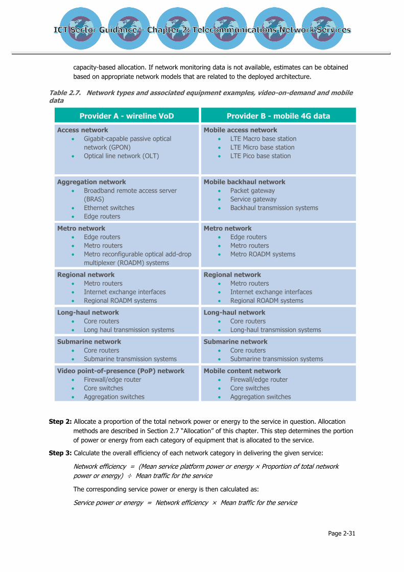
Page 2-31
capacity-based allocation. If network monitoring data is not available, estimates can be obtained
based on appropriate network models that are related to the deployed architecture.
Table 2.7. Network types and associated equipment examples, video-on-demand and mobile data
Provider A - wireline VoD Provider B - mobile 4G data
Access network
Gigabit-capable passive optical
network (GPON)
Optical line network (OLT)
Mobile access network
LTE Macro base station
LTE Micro base station
LTE Pico base station
Aggregation network
Broadband remote access server
(BRAS)
Ethernet switches
Edge routers
Mobile backhaul network
Packet gateway
Service gateway
Backhaul transmission systems
Metro network
Edge routers
Metro routers
Metro reconfigurable optical add-drop
multiplexer (ROADM) systems
Metro network
Edge routers
Metro routers
Metro ROADM systems
Regional network
Metro routers
Internet exchange interfaces
Regional ROADM systems
Regional network
Metro routers
Internet exchange interfaces
Regional ROADM systems
Long-haul network
Core routers
Long haul transmission systems
Long-haul network
Core routers
Long-haul transmission systems
Submarine network
Core routers
Submarine transmission systems
Submarine network
Core routers
Submarine transmission systems
Video point-of-presence (PoP) network
Firewall/edge router
Core switches
Aggregation switches
Mobile content network
Firewall/edge router
Core switches
Aggregation switches
Step 2: Allocate a proportion of the total network power or energy to the service in question. Allocation
methods are described in Section 2.7 “Allocation” of this chapter. This step determines the portion
of power or energy from each category of equipment that is allocated to the service.
Step 3: Calculate the overall efficiency of each network category in delivering the given service:
Network efficiency = (Mean service platform power or energy × Proportion of total network
power or energy) ÷ Mean traffic for the service
The corresponding service power or energy is then calculated as:
Service power or energy = Network efficiency × Mean traffic for the service

Page 2-32
Or:
Service power or energy = Mean service platform power or energy × Proportion of total
network power or energy
This accounts for the bulk differences in equipment use among different services supported by a
network.
Step 4: Calculate the GHG emissions by multiplying the energy used by the appropriate electricity grid
emission factor. Note, if power was determined in the calculations then an additional step will be
required whereby power is converted into energy by multiplying it by the duration of use. Power
averaging may need to be performed based on the equipment type and service performance over
the duration. Where the network covers multiple regions, then either the network should be
subdivided by region or an average electricity grid emission factor should be used.
Bottom-up calculation using the subnetwork composition method
For the bottom-up subnetwork composition method, subnetworks are identified as being composed of
equipment falling into different subnetwork categories. These subnetwork categories can include, for
example, access, aggregation, metro, regional, long haul, and submarine, with each service provider
defining its unique set of subnetworks. The GHG emissions are calculated based on the allocated service
traffic or provisioning and the relative equipment emissions. Below is an example in which the mean traffic
fraction is used for the provisioning factors:
Mean service power or energy = (fraction of power or energy from equipment category 1 ×
Allocation factor for service in equipment category 1) + (Fraction of power or energy from
equipment category 2 × Allocation factor for service in equipment category 2) + Additional
equipment categories…
For additional guidance and calculation methods that may be employed, see the references provided earlier
in this section (Chan et al., 2012, and Kilper et al., 2010).
Bottom-up calculation using the service processing within equipment method
The bottom-up service processing within equipment method, further refines how the service traffic is
handled within the network and also how multiple services are treated within multiple platforms. For
example, some services may traverse more hops through the network and thus accumulate a higher use
fraction than other services. In this case the traffic fraction is weighted by the mean number of hits per
equipment category or mean hit count.17 Below is an example in which the hit-weighted traffic and mean
traffic fraction per equipment category is used for the provisioning factors:
Mean service power or energy = (Fraction of power or energy from equipment category 1 ×
Hit-weighted traffic for equipment category 1 × Mean traffic fraction in equipment category 1) +
(Fraction of power or energy from equipment category 2 × Hit-weighted traffic for equipment
category 2 × Mean traffic fraction in equipment category 2) + Additional equipment
categories…
Note: if all of the equipment in a network reports its traffic by service and its corresponding power or
energy consumption, then the emissions associated with a particular service can be more easily calculated.
17 Note that the term “hit” corresponds to the number of times that a device in a given equipment type is accessed within a
network. This generalizes the notion of a hop count or node count to include intranode hops.

Page 2-33
In these cases, some common equipment shared across services in a provider’s network facilities, such as
air conditioning or network management infrastructure, should be allocated across the services.
If the services receive similar contributions from the common equipment, then an appropriate power
fraction or traffic fraction should be used. For example, network facility air conditioning should use a power
fraction and network management equipment should use a traffic fraction. If a single service uses a
disproportionately large fraction of the common equipment or unique equipment not in the data path (such
as unique control signaling), this equipment should be accounted for separately as appropriate for the
circumstances. For example, an Internet Protocol multimedia subsystem (IMS) service that requires unique
session control hardware should include the power of this hardware in its total service power consumption
at 100 percent use (or added to its corresponding total service power for the platform), even though it may
not show up in traffic trace measurements.
2.9.3 Calculating GHG emissions for the service platform embodied activities
Calculation methods for assessing the embodied GHG emissions (e.g., emissions from the material
acquisition and preprocessing; production; distribution and storage; and end-of-life stages) of equipment
typically found in the service platform are covered in detail in the Hardware Chapter of this ICT Sector
Guidance. Embodied emissions from the service platform equipment may also need to be allocated to the
TNS under study depending on how that equipment shares the service. The allocation procedure can
employ the methods described in Section 2.8.3 “Allocation of customer domain use-stage emissions”.

Page 2-34
2.10 Operational activities
2.10.1 Operational activities overview
Operational activities and non-ICT support equipment covers people (labor)-activities and non-ICT support
equipment and activities that are directly engaged and dedicated to the service being assessed. Table 2.2
provides a full list of attributable and non-attributable processes.
2.10.2 Calculating GHG emissions for the operational activities use stage
Assessment approach
For assessing the GHG emissions of the operational activities use stage, a few alternative approaches can
be used. The most appropriate approach can be selected on the basis of available data and level of
granularity required. The level of granularity required will typically depend on the significance of these
processes to the total life cycle emissions of the service (significance should be determined in the screening
step – see Section 2.5 “Screening”).
Table 2.2 lists the operational activities’ attributable processes. Companies will likely already be measuring
the emissions from these activities and reporting them in corporate GHG inventories. This chapter,
therefore, does not provide data on calculating emissions from facility energy use, vehicle use, and so on.
Instead this chapter provides methods for allocating the service provider’s corporate-level GHG emissions
to the specific service being assessed.
Allocation of operational activity use-stage emissions using employee data
If the company tracks the number of employees dedicated to different services, then the number of
employees dedicated to the service being assessed, as a proportion of total employees, should be used to
allocate the service provider’s GHG emissions. The calculation formula should be:
Operational activities use-stage emissions = (Service provider’s total scope 1 and 2 emissions –
Network and data center emissions) × (Number of employees dedicated to the service ÷ Total
employees)
Allocation of operational activity use-stage emissions using revenue data
If employee data is not available for the service being assessed, then the company’s financial data can be
used to identify the value of a service in terms of its revenue compared with total revenue. This approach
should be used with caution as there is not always a clear relationship between revenues and related
emissions. The calculation formula should be:
Operational activities use-stage emissions = (Service provider’s total scope 1 and 2 emissions –
Network and data center emissions) × (Revenue from the service ÷ Total revenue)
Combining allocated emissions from facilities with primary or estimated data on service-
related employee travel
An alternative approach is to allocate emissions from facilities using one of the allocation methods
described above, and then to collect primary data on or estimate operational activity-related employee
travel and use transport GHG emission factors to calculate emissions from travel.

Page 2-35
Note: it is acknowledged that all these calculation methods use average employee emissions estimates
derived from corporate-level emissions and that the granularity of this approach is coarse as there are
many potential variables: for example, different levels of travel for different job roles. Accuracy of data
could be improved with more detailed analysis and breakdown of specific roles into different allocations of
the company operational emissions, but materiality may not justify this.
If the operational activity use stage is found to be significant within the assessment, it is recommended
that a detailed inventory of labor activities and volumes be compiled and internal financial systems used to
identify the key elements of the activity that give rise to emissions, for example, travel.
Example: Allocating operational activities use-stage emissions with the employee data
method
This example demonstrates a calculation using the service providers’ corporate-level emissions along with
information on the number of employees engaged in the delivery of the service to determine the
operational and non-ICT support equipment emissions.
Total service provider scope 1 and 2 emissions – Network and Data Center emissions = 1,000,000
metric tons CO2e
Total service provider employees = 270,247
Employees engaged in the delivery of the service being assessed = 614
Emissions allocated to the service being assessed = 1,000,000 x (614 ÷ 270,247) = 2,272 metric
tons CO2e
2.10.3 Calculating GHG emissions for the operational activities embodied activities
Embodied GHG emissions (i.e., emissions from the material acquisition and preprocessing; production;
distribution and storage; and end-of-life stages) of operational activities are typically small. This may be
especially so with capital support equipment that is being shared by many network services over long
periods of time. If screening has determined that the embodied emissions of the operational activities are
relatively small, (e.g., less than 1 percent), then it is sufficient to report the emissions calculated by the
screening assessment, without carrying out a more detailed assessment for this element.
If screening methods indicate that embodied emissions of operational activities contribute more
significantly, then a more in-depth assessment should be included to account for these emissions. Refer to
the Product Standard for further guidance on assessing emissions from life cycle stages such as
production, which involves facilities, vehicles, and capital equipment.

Page 2-36
Appendix 2.1: TNS case study: Multiprotocol Label Switching (MPLS) service
Business goals
This case study describes the steps taken by a service provider to assess the GHG emissions of a global
Multiprotocol Label Switching (MPLS) service solution being deployed for a corporate customer to
consolidate its network services onto a single service platform. This activity was carried out in response to
a customer request to assess the GHG emissions of a service proposed to replace its existing network
services.18
As such, this study includes both accounting (back-casting) of existing network entities such as the core
MPLS network and a forward-looking projection of the equipment to be deployed in the customer‘s
premises over the duration of the service, based on the customer’s projected access bandwidth
requirements across its global premises.
Product description
MPLS is an internet protocol (IP) virtual private network service delivering data applications, multimedia,
and IP voice. With multiple distinct classes of service, MPLS allows customers to prioritize traffic based on
application, ensuring that mission-critical data applications are served irrespective of the growth of lower-
priority traffic. MPLS can be classified either as a complex product or a service.
Defining the functional unit
The functional unit for the service in this case study is the use of 10,000 ports with an average capacity
of 1 megabit per second (Mbps) over 63 countries over three years. The service being assessed within
this case study equated to 12.82 percent of the service provider’s total MPLS network service capacity.
The functional unit is based on how the product is sold, that is, the number of ports in the number of
countries over three years and the quality/capacity of service. A port is the physical interface between a
customer device/equipment and a communications network.
Boundary setting
The boundary-setting requirement follows the guidance in this chapter.
Figure A2.5 defines the various service elements and the boundary showing what is included and excluded
in this example.
18 This case study was carried out in 2010 as part of a global customer’s request to understand in more detail the GHG
emissions associated with the provision of a global network service and was used in the pilot study for the Greenhouse Gas
Protocol Product Life Cycle Accounting and Reporting Standard. It was produced prior to the development of this ICT Sector
Guidance and therefore may not follow exactly the detailed guidance provided in this chapter. However, the findings and
experience were used to help develop and shape the methodology and guidance.

Page 2-37
Figure A2.5. The boundary for the MPLS network service being studied
The MPLS network service studied consisted of the following elements:
Customer domain (referred to as customer premises equipment [CPE]) CPE/access ICT and non-ICT network equipment and support equipment
On-ramps (customer data center) ICT and non-ICT network equipment and support equipment
Service platform Core MPLS network — ICT and non-ICT network equipment and support equipment
Global transport network — ICT and non-ICT network equipment and support equipment
Operational activities Operational activities and non-ICT support equipment covers people (labor)-activities and non-
ICT support equipment / support activities, including:
Solution design, surveying, planning deployment / installation, maintenance, and technical
support over the service’s life
Dedicated nontechnical support such as product management, sales, and marketing
Activities associated with decommissioning ICT equipment
The organizational scope 1 and 2 GHG emissions emitted from energy consumed by
facilities/buildings, travel, and transport in undertaking the activities described

Page 2-38
Typical power consumption factor and power usage effectiveness factor used
In this study the practitioner was not able to measure the actual power used by each equipment type in
the service and was unable to obtain typical power consumption data from the vendor. Therefore, to
calculate typical energy consumption a typical power consumption factor (TPCF) of 0.75 (based on
maximum vendor equipment values) was used on all equipment assessed for the study. This assumption
was made based on the guidance in Section 2.8.2 “Calculating GHG emissions for the customer domain use
stage.”
An appropriate factor that accommodates both cooling energy and uninterruptible power supply (UPS)
losses was used based on company expertise and practices. The power usage effectiveness (PUE) metric
was used to model the proportion of electricity required to cool telecommunication equipment to maintain
its proper operation. The MPLS network had a PUE value of 1.7 (i.e., 0.7 watt for every 1 watt consumed
by the telecommunications equipment). This PUE factor was used consistently throughout the study for
calculating the additional power consumption of the equipment cooling systems.
A2.1.1 Customer domain
Customer domain use stage
Steps 1-5 in Section 2.8.2 “Calculating GHG emissions for the customer domain use stage” were followed.
Areas of exception or of note are as follows:
For Step 1: Because this study was for a service that was in the process of being deployed, with the
exception of the on-ramps (customer data center router/local area network (LAN) equipment), accurate
numbers (volumes) of CPE equipment used in each of the locations were not available. Therefore, a
combination of guidance from service design experts and company CPE/access hardware rules were used
to identify the most likely options and numbers (volumes) of equipment required to fulfill the customer’s
requirement based on the number of ports sold. Two scenarios (a maximum and minimum option) were
modeled and an average of the two scenarios was used.
For the on-ramps (data center router/LAN equipment) network, which was already deployed, an accurate
inventory was compiled.
Step 5: Calculate the GHG emissions by multiplying the energy consumption totals by relevant in-country
energy GHG conversion figures to give overall GHG emissions for the customer domain equipment in use.
For the reasons outlined in step 1 (i.e., details of the numbers of equipment used in each location were not
available at this time) a global average energy GHG conversion figure was used for the CPE used in the
customer domain (based on the 63 countries covered by the service).19 For the on-ramps data center
router/LAN equipment that had already been deployed, in-country energy GHG conversion figures were
used.
The following tables A2.8 through A2.11 show the calculations of the GHG emissions for the customer
domain use stage for this case study.
19 An analysis of the service platform emissions, where a detailed equipment inventory for each of the 63 countries was
available, indicated that using a global vs. in-country electricity conversion factor only varied the resultant GHG emissions by
approximately 5 percent.

Page 2-39
Table A2.8. Customer premises equipment: Projected router volume requirements for MPLS service
Average CPE projection
CP
E a
ssu
mp
tion
s
CP
E v
olu
me
s
Po
we
r (W)
Typ
ica
l po
we
r co
nsu
mp
tion
facto
r ap
plie
d (×
0.7
5)
(W)
PU
E a
pp
lied
(× 1
.7) (W
)
En
erg
y/ye
ar (k
Wh
)
En
erg
y /
3 y
ea
rs (k
Wh
)
Glo
ba
l ave
rag
e e
lectric
ity
GH
G e
mis
sio
n fa
cto
r
(kg
CO
2 e/k
Wh
)
GH
G e
mis
sio
ns o
ve
r 3 y
ea
rs
(me
tric to
ns C
O2 e
)
75%
(Class 20) 7,500 50 38 64 4,188,375 12,565,125 0.58 7,338
20% (Class
10/11 mean)
2,000 415 311 529 9,270,270 27,810,810 0.58 16,242
5%
(Class 13) 500 750 563 956 4,188,375 12,565,125 0.58 7,338
Totals 10,000 1,215 911 1,549 17,647,020 52,941,060 0.58 30,919
Assumptions:
For global average electricity emission factors across 63 countries where the points of presence
were located, data from the Carbon Trust Footprint Expert Database was used.
A typical CPE scenario was used with one router per customer MPLS port.
The average scenario assumptions were based on 75% low bandwidth CPE, 20% medium
bandwidth CPE circuits, and 5% high bandwidth CPE circuits. This breakdown was an average of
two scenarios giving maximum and minimum projections of router/circuit requirements. These
scenarios were developed with guidance from service design experts in conjunction with company
CPE/access hardware rules for MPLS detailing classes of equipment/power consumption and
circuit bandwidth requirements.
Note: The equipment classes used in this study are simply a means of anonymizing the identity of different
vendors/types of routers and switches used within the service.

Page 2-40
Table A2.9. Customer premises equipment (CPE)/access hardware rules
Access option Default
equipment Power (W)
Nx64k Leased Line Class 20 50
T1 Leased Line Class 20 50
E1 Leased Line Class 20 50
Ethernet (1) Class 20 50
STM-1 Leased Line Class 11 370
OC-3 Leased Line Class 11 370
E3 Leased Line Class 10 460
T3 Leased Line Class 10 460
Ethernet (2) Class 10 460
Fast Ethernet (1) Class 10 460
STM-4 Leased Line Class 13 750
OC-12 Leased Line Class 13 750
Fast Ethernet (2) Class 13 750
Gigabit Ethernet (250M-1G) Class 13 750

Page 2-41
Table A2.10. Customer premises equipment: Deployed routers (customer data centers – on- ramps)
Site
Ro
ute
r
Qu
an
tity
Ma
x p
ow
er (W
)
Typ
ica
l po
we
r co
nsu
mp
tion
facto
r ap
plie
d (×
0.7
5) (W
)
PU
E fa
cto
r
ap
plie
d (×
1.7
) (W)
Eq
uip
me
nt p
ow
er (W
)
Po
we
r/yr (k
Wh
)
Po
we
r/3
yrs
(kW
h)
Co
un
try e
lectric
ity G
HG
co
nve
rsio
n fa
cto
r
(kg
CO
2 e/ k
Wh
)*
Me
tric to
ns C
O2 e
/
3 y
ea
r lifecycle
UK 1 Class 12
4 259 194.3 330.2 1320.9 11,571 34,713 0.60 20.7
UK 2 Class 12
2 259 194.3 330.2 660.5 5,785 17,356 0.60 10.3
UK 3 Class 12
2 259 194.3 330.2 660.5 5,785 17,356 0.60 10.3
Geneva 1 Class 12
2 259 194.3 330.2 660.5 5,785 17,356 0.03 0.45
USA 1 Class 12
2 259 194.3 330.2 660.5 5,785 17,356 0.67 11.6
USA 2 Class
12 2 259 194.3 330.2 660.5 5,785 17,356 0.67 11.6
USA 3 Class 12
2 259 194.3 330.2 660.5 5,785 17,356 0.67 11.6
USA 4 Class 12
2 259 194.3 330.2 660.5 5,785 17,356 0.67 11.6
Singapore 1 Class 12
2 259 194.3 330.2 660.5 5,785 17,356 0.60 10.4
Singapore 2 Class 12
2 259 194.3 330.2 660.5 5,785 17,356 0.60 10.4
Hong Kong Class 12
2 259 194.3 330.2 660.5 5,785 17,356 0.92 16.0
Tokyo Class 19
2 259 194.3 330.2 660.5 5,785 17,356 0.58 10.1
Total 135.0
* Carbon Trust - Footprint Expert Data

Page 2-42
Table A2.11. Customer premises equipment: Deployed LAN switch equipment (customer data center)
Site
LA
N s
witc
h
Qu
an
tity
Ma
x p
ow
er (W
)
Typ
ica
l po
we
r
co
nsu
mp
tion
facto
r
ap
plie
d (×
0.7
5) (W
)
PU
E fa
cto
r ap
plie
d
(×1
.7) (W
)
Eq
uip
me
nt p
ow
er (W
)
Po
we
r/yr (k
Wh
)
Po
we
r/3
yrs
(kW
h)
Co
un
try e
lectric
ity G
HG
co
nve
rsio
n fa
cto
r (kg
CO
2 e/ k
Wh
)*
Me
tric to
ns C
O2 e
/
3 y
ea
r life c
ycle
UK 1 Class
3 4 2,520 1,890 3,213 12,852 112,584 337,751 0.60 201.0
UK 2 Class
3 2 2,520 1,890 3,213 6,426 56,292 168,875 0.60 100.5
UK 3 Class
3 2 2,520 1,890 3,213 6,426 56,292 168,875 0.60 100.5
Geneva 1 Class
3 2 2,520 1,890 3,213 6,426 56,292 168,875 0.03 4.4
USA 1 Class
3 2 2,520 1,890 3,213 6,426 56,292 168,875 0.67 112.8
USA 2 Class
3 2 2,520 1,890 3,213 6,426 56,292 168,875 0.67 112.8
USA 3 Class
3 2 2,520 1,890 3,213 6,426 56,292 168,875 0.67 112.8
USA 4 Class
3 2 2,520 1,890 3,213 6,426 56,292 168,875 0.67 112.8
Singa-pore 1
Class 3
2 2,520 1,890 3,213 6,426 56,292 168,875 0.60 100.9
Singa-pore 2
Class 3
2 2,520 1,890 3,213 6,426 56,292 168,875 0.60 100.9
Hong Kong
Class 3
2 2,520 1,890 3,213 6,426 56,292 168,875 0.92 155.8
Tokyo Class
3 2 2,520 1,890 3,213 6,426 56,292 168,875 0.58 97.9
Total 1,313.3
* Carbon Trust - Footprint Expert Data
Customer domain use stage total emissions were calculated as in Tables A2.8 through A2.11:
Customer domain use-stage GHG emissions total = 30,919 + 135 + 1313 = 32,367 metric tons CO2e
(over 3-year service).
Customer domain embodied stage
Because the processes in this stage were not under operational or financial control of the reporting
company, use of secondary data is in conformance with the Product Standard.
Of the two options recommended (the life cycle stage ratio modeling or the economic input/output
assessment), the latter was used initially because capital expenditure (CAPEX) data was available for the
MPLS network over the period of the service. This CAPEX value was allocated using provisioned capacity in
terms of number of ports dedicated to the assessed telecommunications network services (TNS) (i.e., as a

Page 2-43
percentage of case study network capacity to total network capacity) and then used in conjunction with the
environmentally-extended input-output (EEIO) data tables provided by the UK Department for
Environment, Food and Rural Affairs (Defra) to estimate the embodied GHG emissions for the network.
The case study service represents 12.82 percent of the calculated total service provider’s MPLS network
platform port capacity. A cost-based approach using internal CAPEX data to build the MPLS network was
used and a 12.82 percent proportion of this over three years was determined to account for the case study
service. This gave an allocated value of £11.538 million over three years.
This allocated value was then input into the Defra EEIO table to calculate the embodied emissions from the
production of the MPLS equipment and non-ICT support equipment (e.g., cabling and racking). A detailed
breakdown of the CAPEX by product category was not available; therefore, an average value across three
product categories detailed within the Defra EEIO tables was used. These product categories offered the
closest match to the range of equipment, products, and services that make up the TNS. This was
calculated as shown in Table A2.12.
Table A2.12. Calculating total embodied emissions of the network using the economic data method
Product type Amount spent by product type
(£ millions)
EEIO emission
factor
(kg CO2e per £)
Total emissions
(metric tons CO2e)
Office machinery and
computers 11.538 x 0.58 6,696
Radio, television, and
communications 11.538 x 0.56 6,488
Post and telecommunications 11.538 x 0.37 4,244
Averaged emissions (product categories above) 5,809

Page 2-44
Calculating total embodied emissions of the network using the life cycle ratio method
In addition to the economic method described above, a second calculation approach using secondary data
— called life cycle stage ratio modeling — was subsequently used to ensure reasonable levels of confidence
in the values obtained. Here the use-stage GHG emissions can be modeled as a percentage of the total life
cycle GHG emissions, accounting for the equipment type, usage profile, and country/region of usage. The
ratios were developed based on historical life cycle assessments for different ICT equipment types.
For this analysis, steps 1-5 of the customer domain embodied stage assessment approach detailed in this
chapter were followed. The underlying process is described in more detail in the Hardware Chapter.
Table A2.13. Examples of TNS equipment life cycle stage guidance
Category Product types Typical physical
configuration
Assumed usage profile
(on/standby/off)
Typical lifetime (years)
Life cycle stage ratio
Use
stage Embodied
C-1 LED / LCD monitors Various types / sizes 7.2/2.4/14.4 x 5 3 20% 80%
C-2 Mobile phone Various types 20 minutes/day (voice)
2 30% 70%
C-3 Personal Computer 30% 70%
Small laptop PC Various types 7.2/2.4/14.4 x 5 4
Widescreen laptop PC Various types 7.2/2.4/14.4 x 5 4
Desktop PC Various types
Tablet PC Various types
C-4 Set top box (STB) Various types 18 / 6 / 0 3 80% 20%
C-5 Voice-over-internet Protocol (VoIP) phone
Various types 24 x 7 10 90% 10%
Analog telephone adapters (ATA) / VoIP gateway
Various types 24 x 7 10 90% 10%
C-6 Home gateways – Central functions plus wide-area network (WAN) interface
Processor, memory, WAN interface
24 x 7 3 80% 20%
Digital subscriber line (DSL) customer premises equipment (CPE)
ADSL, ADSL2, ADSL2+, VDSL2
WAN Fast, Gigabit, and Fiber PtP
Fast, Fiber PtP Gigabit Ethernet
B-5 Routers 10
Router - small chassis/blade
2 slots 24 x 7 85% 15%
Router - medium chassis/blade
3-6 slots 24 x 7 85% 15%
Router - large chassis/blade
9+ slots 24 x 7 95% 5%
Router - standalone, small
1 RU, including wireless 24 x 7 85% 15%
Router - standalone, medium
2 RU 24 x 7 85% 15%
Router - core 24 x 7 90% 10%

Page 2-45
In Table A2.13 product types are divided into categories (e.g., C-4 Set Top Boxes, B-5 Routers) with
similar lifespan and percentages of use and embodied GHG emissions based on historic life cycle
assessment (LCA) studies of these equipment types. This table can be used to assist in the calculation of
embodied emissions of equipment where the use-stage emissions are known for particular types of
equipment.
An example of this calculation for a small standalone router (defined as class 20 in this study) is as follows:
Using these tables, the majority of the routers (classes 20, 10, 11 and 13) fall within the B-5 Router -
standalone, small and B-5 Router - standalone, medium categories. Using the class 20 type as an example,
which has a typical active power consumption of 50W, this equates to 63.75W, taking into consideration a
TPCF of 0.75 and a PUE factor of 1.7, as used for calculating the use-stage emissions. With a duty cycle of
8,760 hours and a life expectancy of seven years, its use-stage emissions should be:
Euse = 63.75 W × 8,760 hours/yr × 7 yrs × 1 kWh/1,000 Wh × 0.584 kg CO2e/kWh*
(*Electricity emission factor for global average across the regions of use)
Thus: Euse = 2,283 kg CO2e (use-stage GHG emissions)
Using the life cycle stage percentages given in Table A2.13, the router’s embodied GHG emissions should then be estimated to be:
Eembodied = [2,283 kg CO2e ÷ (85/100)] × [1 – (85/100)]
Thus: Eembodied = 403 kg CO2e (embodied stage GHG emissions)
As all the equipment in the case study had a lifespan of seven years and a service contract of only three
years, it is expected (from company policy) that the equipment would be reused/resold for other contracts.
To account for the appropriate amount of embodied emissions for the case study, an allocation factor of
3/7 was used for all equipment.
Thus: Eallocated embodied = 403 kg CO2e × (3 ÷ 7) = 172.7 kg CO2e
It was estimated that 7,500 Class 20 routers would be deployed in the service.
Therefore, this would give a value for the total embodied emissions of:
7,500 × 172.7 kg CO2e = 1,295,357 kg CO2e (1,295 metric tons CO2e)
Similar calculations were made for all the other classes of routers used. These are shown in Table A2.14.

Page 2-46
Table A2.14. Average Customer Premises Equipment (CPE) projection
Average CPE projection
Use-stage GHG emissions Embodied
GHG emissions
CP
E a
ssu
mp
tion
s
CP
E v
olu
me
Po
we
r pe
r CP
E ite
m (W
)
typ
ica
l po
we
r co
nsu
mp
tion
facto
r ap
plie
d (x
0.7
5) (W
)
PU
E a
pp
lied
(x 1
.7) (W
)
To
tal C
PE
vo
lum
e e
ne
rgy/ye
ar
(kW
h)
To
tal C
PE
vo
lum
e e
ne
rgy
/
3 y
ea
rs
(kW
h)
Glo
ba
l ave
rag
e e
lectric
ity
GH
G e
mis
sio
n fa
cto
r
(kg
CO
2 e/k
Wh
)
To
tal C
PE
vo
lum
e G
HG
em
issio
ns/3
ye
ars
(me
tric to
ns C
O2 e
)
Em
issio
ns p
er ite
m o
f CP
E
/ 3
ye
ars
(me
tric to
ns C
O2 e
)
To
tal C
PE
em
issio
ns - a
lloca
ted
ove
r 3 y
ea
rs (m
etric
ton
s C
O2 e
)
75%
(Class 20) 7,500 50 38 64 4,188,375 12,565,125 0.58 7,338 0.173 1,295
20% (Class
10/11 mean)
2,000 415 311 529 9,270,270 27,810,810 0.58 16,242 1.214 2,427
5%
(Class 13) 500 750 563 956 4,188,375 12,565,125 0.58 7,338 2.193 1,097
Totals 10,000 1,215 911 1,549 17,647,020 52,941,060 0.58 30,919 --- 4,819
Thus, the CPE-embodied GHG emissions is 4,819 metric tons of CO2e.
The same approach was applied to the on-ramps (as well as core platform and global transport equipment
— see service platform embodied calculations, below).
The network on-ramp embodied GHG emissions is 215 metric tons CO2e.
Therefore, total embodied GHG emissions for customer domain is (4,819 + 215) or 5,034 metric tons
CO2e.

Page 2-47
A2.1.2 Service platform
The service platform comprised the following elements, which supported the MPLS service offering:
Global core network, which comprised the switching and routing equipment located at core MPLS
network nodes around the world.
Global transport network, which comprised a number of equipment platforms including subsea
systems used to provide interconnectivity across core, access, and customer domain MPLS nodes.
Service platform use stage
Although a detailed bottom-up hardware inventory for both the global MPLS core and transport networks
was possible, a top-down approach was used to calculate the emissions allocated to the case study service.
By following steps 1-5 described earlier for customer domain equipment, the power usage and GHG
emissions for the total service platform were evaluated. To evaluate the fraction of the core platform
emissions used by the case study example, these emissions were then allocated based on provisioned
capacity compared with the total capacity.
Calculating use-stage emissions for the global MPLS core network
Steps 1-5 of the service platform use stage of the TNS guide were followed. Areas of note or exception
are as follows:
Step 1: Compile inventory of equipment — Categories of equipment (e.g., routers, switches): 18 classes of
equipment were identified. Total pieces of equipment = 3,136
The total number of each category of equipment at each node location in each country was identified.
For this study, the manufacturer’s technical data provided only maximum power consumption for each
equipment type/category. Therefore a TPCF of 0.75 was used to obtain typical power use.
Step 2: The service platform networks are used for 24 hours of every day of each year of service. In this
case the usage profile is: 24 hours per day; for 365 days per year; for 3 years of service.
Step 3: A PUE factor of 1.7 was used for all equipment power consumption / energy use.
Table A2.15 shows an extraction of how this data was captured and calculated for steps 1 to 4.

Page 2-48
Table A2.15. Calculating use-stage energy consumption for the global MPLS core network
Site/equipment types
Class 1 Class 2 Classes 3...17
Class 18 Totals
AF 1 0 … 0 41
AM 15 2 … 0 658
AP 23 0 … 0 527
EU 37 2 … 7 1,833
ME 2 0 … 0 77
Total number of
equipment units 78 4 … 7 3,136
Max power (kW) 1.13 1.30 … 5 35.78
Power (kW)
(after applying a
TPCF of 0.75)
0.85 0.98 … 3.83 26.84
Power (kW)
(after applying a
PUE factor of 1.7)
1.44 1.66 … 6.50 45.62
Total equipment
power (kW) 113 7 … 46 3,632
In-use energy for
service (24x365x3)
(kWh)
2,961,148 174,236 … 1,196,200 95,451,190
Step 5: Calculate the GHG emissions by multiplying the energy consumption totals by relevant grid
average electricity emission factors to give overall GHG emissions for the core MPLS network equipment
use stage. Table A2.16 shows an extract of how this data was captured and calculated for step 5.

Page 2-49
Table A2.16. Calculating use-stage emissions for the global MPLS core network
Site
Re
gio
n
Co
un
try
City
Co
un
try e
lectric
ity G
HG
em
issio
n
facto
r (kg
CO
2 e/k
Wh
)
Eq
uip
me
nt c
lass 1
(nu
mb
er o
f un
its d
ep
loye
d)
Eq
uip
me
nt c
lasse
s 2
....17
Eq
uip
me
nt c
lass 1
8
(nu
mb
er o
f un
its d
ep
loye
d)
To
tal c
ore
MP
LS
pla
tform
in-u
se
ele
ctric
ity c
on
su
mp
tion
over 3
ye
ars
(kW
h)
To
tal c
ore
MP
LS
pla
tform
GH
G
em
issio
ns
ove
r 3 y
ea
rs
(me
tric to
ns C
O2 e
)
BAW-AM
AM Argentina Buenos Aires 0.4225627 1 … 0 133,793 19
BDA-
AM AM Argentina Buenos Aires 0.4225627 2 … 2 509,843 72
BUE-
AM AM Argentina Buenos Aires 0.4225627 2 … 0 243,797 34
MEL-AP
AP Australia Melbourne 0.9429827 1 … 2 623,331 196
MLL-AP
AP Australia Melbourne 0.9429827 0 … 0 12,398 4
SPT-
AP AP Australia Sydney 0.9429827 1 … 2 809,965 255
SYD-AP
AP Australia Sydney 0.9429827 0 … 0 12,398 4
SYT-AP
AP Australia Sydney 0.9429827 1 … 0 289,266 91
VIE-
EU EU Austria Vienna 0.2254179 0 … 2 566,938 43
VII-
EU EU Austria Vienna 0.2254179 1 … 0 500,360 38
… … … … … … … … … …
WDV-
AM AM
United
States Washington
DC 0.668203 0 0 49,590 12,398
SGN-AP
AP Vietnam Ho Chi Minh City
0.4450243 0 0 148,323 37,081
… … … … … … … … … …
Total 78 122 95,451,190 52,515
Note: AM=America, AP=Asia Pacific, EU=European Union
Calculating use-stage emissions for the global transport network
Using the steps described above, the equipment inventory, power consumption and GHG emissions were
evaluated across the global nodes of the four network platforms, which are used to transport MPLS.
First, the total emissions per annum were calculated for these platforms. As in previous calculations, a
TPCF of 0.75 was applied to the maximum power consumption of each equipment listed along with a PUE

Page 2-50
factor of 1.7. A global average electricity grid conversion factor was used (as described in the customer
domain section) to calculate the GHG emissions.
Internal network models were used to determine the proportion of circuit capacity required by MPLS across
these platforms. These values were used to allocate the total GHG emissions for MPLS.
A second allocation was subsequently used to assign the relative proportion of the overall MPLS emissions
for the service detailed by the functional unit for this case study. This is described in Table A2.17 and in
the text below.
Table A2.17. Calculating use-stage emissions for the global transport platforms carrying MPLS traffic
MPLS allocation of GHG emissions across global transport platforms
Platform – in-use electricity GHG emissions
CO2e / yr (metric tons)
CO2e / 3 yrs (metric tons)
Platform 1 329 988
Platform 2 1,040 3,120
Platform 3 224 672
Platform 4 368 1,105
Grand Total 1,962 5,885
To allocate a proportion of total emissions of the service platform to the service being assessed in this case
study, a ratio of provisioned bandwidth capacity used by the service compared with the total bandwidth
capacity of the service platform was used.
The service was for the use of 10,000 ports with an average capacity of 1Mbps across 63 countries. This
accounted for 12.82 percent of the core MPLS network capacity. Therefore an allocation factor of 12.82
percent of the total core MPLS network GHG emissions from electricity consumed was used to estimate the
core network and global transport network use-stage emissions over the three-year period of the case
study example.
Total core MPLS network GHG emissions from electricity usage over three years were 52,515 metric tons
CO2e. The proportion of provisioned core MPLS network capacity used by the case study service is 12.82
percent. Therefore, GHG emissions used by the case study service over the core MPLS network in three
years are:
52,515 x 12.82% = 6,732 metric tons CO2e
Total GHG emissions from electricity usage across the global transport network platforms carrying MPLS
network services over three years is 5,885 metric tons CO2e.
The proportion of the provisioned global transport network capacity carrying MPLS network services
allocated to case study service is 12.82 percent. Thus:
5,885 x 12.82% = 754 metric tons CO2e
Therefore, the total use-stage emissions for the service platform is (6,732 + 754) = 7,486 metric tons
CO2e

Page 2-51
Service platform embodied emissions stage
Estimating service platform embodied emissions stage using life cycle stage ratio profiling
A screening estimate was initially carried out as detailed in Section 2.5 using secondary data from existing
life cycle assessment studies to estimate emissions.
The published life cycle assessment analysis of a GSM (global system for mobile communications) network
was used (analysis was conducted by the original equipment manufacturer (OEM)) and indicated that the
communications solution was comprised of approximately 20-30 percent embodied GHG emissions and 70-
80 percent use-stage GHG emissions). Based on this and other publications, a ratio of 25 to 75 percent of
embodied- to use-stage GHG emissions was used. Knowing the use-stage emissions of the service platform
as detailed above, it was possible to use this figure to estimate the embodied emissions. Thus:
7,486 × (25% ÷ 75%) = 2,495 metric tons CO2e
Therefore the embodied emissions are 2,495 metric tons CO2e.
While this approach and result were useful for providing an initial screening estimation, the secondary data
was not technologically representative of the MPLS TNS in this case study because the profile was for a
mobile communications system. Therefore, the result has a high level of uncertainty so more accurate
approaches using secondary data, such as economic data, were carried out.
Estimating service platform embodied emissions using economic data
A further calculation was made using CAPEX data for the whole MPLS network service as described
previously in the customer domain embodied emissions stage section.
Using this approach, a relative proportion of the embodied emissions (based on the proportion of total use-
stage emissions (18.8% x 5,809 metric tons CO2e) for the service platform was estimated as 1,091 metric
tons CO2e.
The CAPEX data is considered to be more accurate, but there was uncertainty over the averaging across
product categories and the level of granularity is generally low compared with other sources of data. The
CAPEX data also does not include the global transport network (this is not part of MPLS CAPEX as it is a
separate network platform). In addition, this approach considers only supply-chain emissions and does not
include end-of-life emissions. Therefore, the previous data source (lifecycle analysis of a GSM network) was
used to estimate whether end-of-life GHG emissions were significant.
End-of-life considerations
End-of-life processes other than reuse are not under the operational/financial control of the reporting
company and therefore use of secondary data was considered satisfactory. References found on life cycle
GHG emissions studies of ICT equipment and network services as part of the initial screening analysis
indicate that the impacts in terms of GHG emissions tend to be very small and sometimes negative if a
recycling credit is applied to the raw materials acquisition and preprocessing stage.20 The end-of-life stage
typically represents only -0.5 to -2 percent of a service’s total GHG emissions. This is because of the high
level of recycling of network equipment.
In addition, company policy requires that all equipment, at the end of a service period, be reused or
recovered to extend its service life as long as possible. If this is not possible, the equipment is broken
down for material and component recycling by a third party waste management company.
20 The Product Standard has reporting requirements for recycling to avoid reporting negative values.

Page 2-52
A hierarchical approach is adopted whereby equipment is evaluated and the most appropriate action taken,
with reassignment to another service within its current location being the most preferred option. If
reassignment is not possible, the equipment is transported to a location where it can be reused or
alternatively be either resold or refurbished for use elsewhere.
This practice should mean that the majority of ICT hardware continues to be used for much longer than
the three-year service period, minimizing end-of-life emissions. Because only a high-level assessment using
low-quality secondary data in terms of technological representativeness was carried out, a precautionary
approach was adopted to leave the figure at zero.
Life cycle stage ratio modeling:
As there was a discrepancy between the two estimation techniques, a third estimation was carried out
using the life cycle stage ratio modeling approach using better quality secondary life cycle data (in terms of
technological representativeness). The calculation approach and steps undertaken are the same as those
detailed and carried out in the customer domain embodied emissions section using the service platform
equipment inventory (classes 1 to 18 of equipment) detailed in the use-stage section (Table A2.15). This
method produced the following results:
Core MPLS service network = 932 metric tons CO2e
Global transport network = 133 metric tons CO2e
Service platform total = 1,065 metric tons CO2e
It was concluded that because the CAPEX data covered both ICT and support equipment, it would be used.
However, as it did not include the embodied emissions for the global transport network, the values from
the life cycle ratio approach would be used for that element.
Combining the two approaches for the different platforms gave the following results:
Core MPLS service network = 1,091 metric tons CO2e
Global transport network = 133 metric tons CO2e
This gives a service platform embodied GHG emissions total: 1,091 + 133 = 1,224 metric tons
CO2e
A2.1.3 Operational activities
Operational activities and non-ICT support equipment covers people (labor)-activities and non-ICT support
equipment / support activities that are directly engaged and dedicated to the service being assessed,
including design, surveying, planning, logistics, deployment / installation, maintenance, and technical
support.
Operational activities boundary setting
The operational activities boundary setting as detailed in this chapter was used.
Operational activities use stage
Assessment approach
The service provider had already carried out a corporate GHG inventory, measuring the emissions
associated with the operational activities of the whole company using primary data (as this was under
the control of the operating company). This survey included estate electricity (buildings lighting,
heating/cooling, and office ICT equipment, excluding network), travel and commercial fleet fuel use and
natural gas (building heating). The quantity of emissions was first allocated to the total MPLS service
operated by the service provider. For this, the employee data allocation method was used to account
for the number of people employed on the total MPLS service (see Section 2.10.2) for further details on
calculation approach).

Page 2-53
Total MPLS operational activities use-stage emissions = (Service provider’s total scope 1 and 2
emissions – Network and data center emissions) × (Number of employees dedicated to total MPLS
service ÷ Total employees)
Service provider’s total scope 1 and 2 emissions – Network and data center emissions = 227,601.786 metric tons CO2e/year
Number of employees dedicated to the service ÷ Total employees = 0.028
Total MPLS operational activities use-stage emissions = 227,601.786 metric tons CO2e/year x 0.028 =
6,372.85 metric tons CO2e/year
A second allocation is then required to calculate the operation use-stage emissions for the specific service
offering being assessed within the overall MPLS service. For this, the company does not gather data that
would enable the number of people engaged on the service being assessed to be captured accurately. As a
result, the employee data allocation method could not be used. However, the company does know the
proportion of the company’s MPLS network platform port capacity used by the service being assessed
(12.82 percent, as described above). Therefore the network capacity allocation method was used.
The service provider’s operational activity emissions related to the service being assessed is:
Operational activity use-stage emissions = Service provider’s total MPLS operational activity emissions
× 12.82% = 6,372.85 × 12.82% = 817 metric tons CO2e/year
Over a three-year service contract this equates to operational activities use-stage GHG emissions of
2,451 metric tons CO2e
Operational activities embodied stage
Embodied GHG emissions (e.g., emissions from the material acquisition and preprocessing; production;
distribution and storage; and end-of-life stages) of operational activities was excluded as it was determined
through a screening analysis that the impact was relatively small, e.g., less than 1 percent.
A2.1.4 Summary
Table A2.18 shows the total GHG emissions for the MPLS service case study example as well as the
breakdown for the different life cycle stages and TNS elements.
Table A2.18. MPLS Service GHG summary and inventory by life cycle stages and TNS elements
TNS element Life cycle
stage GHG emissions
(metric tons CO2e)
Customer domain Use 32,367
Embodied 5,034
Service platform Use 7,486
Embodied 1,244
Operational activities Use 2,451
Embodied Negligible
Grand total 48,582

Page 2-54
Figure A2.6 shows total emissions broken down by the constituent elements of the MPLS network used by
the case study service.
Figure A2.6. GHG emissions calculated for the MPLS service
A2.1.5 Remarks
The inventory results indicate that the customer domain element (and in particular its use stage) is the
most significant source of emissions for the case study service, with network services platform and
operational emissions being much less significant. Therefore, it can be concluded that additional data-
collection efforts should focus on the customer domain use-stage emissions. The use of secondary data is
adequate for the less significant emission sources, that is the service platform embodied emissions and
operational activities.
0
5,000
10,000
15,000
20,000
25,000
30,000
35,000
40,000
45,000
Customerdomain
Serviceplatform
Operationalactivities
Total
met
ric
ton
s C
O2e
/3
yea
rs
Embodied GHG emissions
Use stage GHG emissions

ICT Sector Guidance built on the
GHG Protocol Product Life Cycle Accounting and Reporting Standard
Chapter 3: Guide for assessing GHG emissions of
Desktop Managed Services
July 2017
This Guidance has been reviewed for conformance with the GHG Protocol Product Standard.

Page 3-2
Contents
Chapter 3: Guide for assessing GHG emissions of Desktop Managed Services ....................................... 3-1 3.1 Introduction ..................................................................................................................... 3-4
3.1.1 What is in this chapter ................................................................................................... 3-4 3.1.2 How to use this guidance ............................................................................................... 3-4 3.1.3 The audience for this chapter ......................................................................................... 3-4 3.1.4 Examples: When to use and when not to use this chapter ................................................ 3-4 3.1.5 Rationale for providing sector guidance for DMS .............................................................. 3-5
3.2 Establishing the scope of the product inventory ................................................................... 3-5 3.3 Defining the functional unit ................................................................................................ 3-6 3.4 Boundary setting ............................................................................................................... 3-8
3.4.1 Introduction .................................................................................................................. 3-8 3.4.2 Defining life cycle stages and identifying attributable processes ........................................ 3-9 3.4.3 Developing a process map ........................................................................................... 3-10 3.4.4 Non-attributable processes .......................................................................................... 3-12 3.4.5 Time boundary............................................................................................................ 3-12 3.4.6 Technical refresh ......................................................................................................... 3-12
3.5 Allocation ........................................................................................................................ 3-12 3.6 Collecting data and assessing data quality ......................................................................... 3-14
3.6.1 Data collection approach .............................................................................................. 3-14 3.6.2 Data collection requirements ........................................................................................ 3-14
3.7 Calculating GHG emissions ................................................................................................ 3-17 3.8 Example of calculating the GHG emissions ......................................................................... 3-18
Tables
Table 3.1. Recommended allocation methods for shared components ............................................... 3-13
Table 3.2. Data requirements for the GHG assessment of DMS ......................................................... 3-15
Table 3.3. Example of emissions from usage of end-user devices ...................................................... 3-21
Table 3.4. Example of emissions from usage of end-user infrastructure ............................................. 3-23
Table 3.5. Example of summary of emissions by stage ..................................................................... 3-24
Figures
Figure 3.1. The elements that make up DMS .................................................................................... 3-5
Figure 3.2. The five stages of a product life cycle ............................................................................. 3-9
Figure 3.3. Example process map showing the five key life cycle stages for DMS .............................. 3-11

Page 3-3
Executive Summary: Desktop managed services
Desktop managed services (DMS) are provided by specialist information and communication technology
(ICT) companies to businesses to manage their desktop environments (such as personal computers,
laptops, tablets, and smartphones). DMS can include different ranges of services, but usually include the
provision of the desktop end-user equipment, the supporting infrastructure of networks and servers, and
the management and support of the service including maintenance services, service desk, and software
upgrades. DMS are a common outsourcing service in many countries.
This chapter provides:
Overall guidance to calculate the greenhouse gas emissions related to DMS.
Guidance on defining the elements that make up DMS, helping the practitioner clearly define the
scope of the DMS to be assessed. Examples of DMS are provided showing the different scopes
that DMS may cover. Also guidance is given on defining the functional unit for DMS. Typically, the
functional unit should state the magnitude (e.g., number of users), the duration (e.g., length of
service), and the quality (e.g., type of support, response times).
Discussion of how to define the boundary for DMS and map the product life cycle stages to the
different DMS processes, including an example process map. Boundary setting includes the
definition of attributable and non-attributable processes (i.e. what is included or excluded from
the boundary definition).
Guidance on allocation methods for different shared components. This is important as DMS
increasingly use shared infrastructure and support arrangements, for example, shared networks,
shared hardware (especially servers and cloud based computing), and shared support services.
Guidance on typical data requirements for the different life cycle stages. A table provides
examples of data sources and notes for the different stages of DMS.
The chapter concludes with guidance on calculating the greenhouse gas emissions from DMS with a
worked example.

Page 3-4
3.1 Introduction
3.1.1 What is in this chapter This chapter forms part of the ICT Sector Guidance, built on the Greenhouse Gas Protocol Product
Life Cycle Accounting and Reporting Standard (Product Standard) and covers desktop managed
services (DMS).
It provides guidance and accounting methods for the calculation of GHG emissions related to DMS.
The chapter provides guidance on the following key items:
Establishing the scope of a product inventory (including a working definition for DMS)
Defining the functional unit
Boundary setting (including mapping the product life cycle stages)
Allocation
Collecting data and assessing data quality
Calculating inventory results and GHG emissions (including a worked example)
3.1.2 How to use this guidance
The purpose of this Sector Guidance is to provide additional guidance to practitioners who are
implementing the Product Standard for ICT products (including ICT services). This Sector Guidance follows
a life cycle approach to the assessment of ICT products (including services). The ICT Sector Guidance is a
supplement to the Product Standard, and thus assumes that the reader is familiar with the principles and
content of the Product Standard. The ICT Sector Guidance is divided into chapters, with general guidance
provided in the Introduction Chapter, and specific guidance in each of the subject chapters. The chapters
cover the following subjects: Telecommunications Network Services; Desktop Managed Services; Cloud and
Data Center Services; Hardware; and Software.
This chapter should be used in conjunction with the Introduction Chapter and with the Product Standard.
3.1.3 The audience for this chapter
There are several potential users of this chapter:
Suppliers of DMS, who require standard terminology, guidance, and accounting methods to
calculate the GHG emissions of the DMS they provide. This may often be required in response to
queries from their customers and potential customers. The calculations can also be used to
understand the sources of the major GHG emissions from DMS, and how the suppliers may reduce
the emissions of the services they provide.
Companies that are users of DMS. Companies may require a common approach to the
calculation of GHG emissions when considering different DMS. It may also be useful if considering
in-house vs. outsourced provision of DMS.
Policymakers, who need a consistent approach to calculating the GHG impact from DMS in order
to understand it in the context of the wider impact of Information and Communication Technology
(ICT).
Consultants, who are tasked with calculating the GHG emissions of DMS on behalf of their
clients.
Nongovernmental organizations (NGOs) and advocacy groups that are addressing the
impact of ICT on climate change, and need a consistent approach to calculating the GHG impact
from DMS.
3.1.4 Examples: When to use and when not to use this chapter
This chapter assumes that DMS are provided by a third party organization to the company using the DMS.

Page 3-5
It may be used where an external third party is providing (or intends to provide) DMS to a
company.
It may also be used where a company is providing DMS in-house to itself. In this case, it is
important to explicitly state the boundary of the system and services that are being provided.
It may be used to assess the impact of different configurations of DMS.
As with the Product Standard, this chapter is not intended to support product comparisons among
different DMS. Further guidance on product comparisons is provided in the Product Standard
(section 1.5 and appendix A).
3.1.5 Rationale for providing sector guidance for DMS
The ICT services included in this ICT Sector Guidance have been chosen largely on grounds of high
customer demand and of broadness of coverage. DMS meet both criteria because they form a large portion
of the ICT services delivered and required within business and, by their nature, comprise many underlying
ICT building blocks, such as desktop/laptop hardware, local area networks (LANs), wide-area networks
(WANs), data-center-hosted servers and other equipment, and ancillary services such as help desk and
deskside support.
Some of these building blocks are defined in other chapters (e.g., the Hardware Chapter) of this ICT Sector
Guidance. They are referenced in this chapter as appropriate to the context.
3.2 Establishing the scope of the product inventory Desktop managed services (DMS) are provided by specialist ICT companies to businesses to manage their
desktop environments (such as personal computers (PCs), laptops, tablets, and smartphones). DMS can
include different ranges of services, but usually include the provision of the desktop end-user equipment,
the supporting infrastructure of networks and servers, and the management and support of the service
including maintenance services, service desk, and software upgrades. Our definition of DMS is aligned to
the Gartner1 definition, which shows they can be broken down into some or all of the elements shown in
Figure 3.1.
Figure 3.1. The elements that make up DMS
1 http://www.gartner.com/id=1450113

Page 3-6
The service desk includes (where provided) incident, problem, change, and release management and a
single point of contact for all IT issues. The service desk may also provide remote assistance to users, and
can manage and maintain any user self-service provision — allowing users to fix common IT issues (such
as password lockouts) without the need to log a call.
The end-user device service covers the provision and management of the desktop devices, including
desktops, laptops, thin client terminals, and mobile devices through the full life cycle stages (see Figure
3.2). During the device lifetime, the latest configuration management tools can be used to ensure a
common standard across the IT estate and ensure the device is kept up to date with the latest security
enhancements. This element may also include advanced third and fourth line (remote) support for desktop
issues. End-user devices include laptops, desktops, and services that are not covered in other segments
such as deskside services or service desk (e.g., software builds, third and fourth line support).
Deskside services ensure that users have the right level of support, wherever they may be. If remote
assistance by the service desk (where provided) is not enough, deskside support teams can visit the end-
user to help resolve software issues; provide hardware fixes or replacements; or provide support for any
planned upgrades, changes, or moves as required.
The end-user infrastructure service can include the hosting (if required), management, and ongoing
optimization of the infrastructure that supports the desktop service. This may include directory, email, file
and print, mail relay, security, and internet proxy services. The service can encompass elements expected
from a comprehensive infrastructure management service including operating system and application
updates, service backup and restore, availability management, capacity management, performance
management, software and hardware support. This component can also include management and support
for the desktop printer infrastructure.
Service delivery management can include service-level management, service reporting, strategies for
continuous improvement, and providing a single point of authority and management interaction dedicated
to ensuring quality of service.
3.3 Defining the functional unit The functional unit of DMS is the provision of a defined amount of desktop services to a number of
supported users for a specified time period. This relates to how DMS are usually priced and sold by
vendors.
In establishing the functional unit, service providers should define the following three parameters:
The quantity of the service: Typically the number of users supported, and:
For each user or user group a list of supported devices
Expected tickets per user (requests and incidents)
Note that the number of users is likely to fluctuate throughout the year and may change from year to year.
Therefore, a weighted average of the number of users per year should be used; if there is a significant
change from one year to the next, the emissions should be recalculated and restated.
The duration of the service: This is the length of service and may be expressed as the life of the
contract or per year (or both measures may be used), and should include:
Whether there is a refresh planned either prior to, or during the service
The usage profile within the time period (e.g., office hours)
The quality of the service: This describes the service levels that apply for the service and will typically
include:

Page 3-7
The type of engineering support (e.g., on site, mobile)
The response/fix times for the support service (e.g., service desk, engineering)
The geography of the service should also be considered and whether the service is delivered over several
countries/geographies. However, this is covered under the calculation where the (consistent) energy
output is varied by the emission factor for each country.
The calculation should take into account all of these variables.
The quantity, quality, and duration parameters are all based on the technical performance characteristics
and service life of the DMS that is being assessed.
Below are two examples of DMS that demonstrate the breadth of possibility in terms of DMS. Many
permutations of DMS are possible.
Example 1:
Quantity
5,000 users in total, split as follows:
a. 2,500 users office based (each with a desktop)
b. 2,500 users mobile (each with a laptop)
Average of 1 ticket per user per month (split 0.25 / 0.75 requests/incidents)
Five office locations (all UK) – 500 users in each
Duration
Five-year contract
Usage profile/hours of support cover – office hours: 08:00–18:00 Monday to Friday
Quality
Local desktop engineering teams at each office
Mobile desktop engineering teams supporting mobile laptop users
Dedicated service desk (housed in one of the five UK locations) – 24 x 7 service
Local IT infrastructure
Standard service-level agreements (SLA) (see below on explanations on how service levels can
impact the environmental aspects of DMS)
Example 2:
Quantity
10,000 users total, split as follows:
a. UK:
i. 1,000 users office based (each with a desktop)
ii. 1,000 users mobile (each with a laptop)
b. France:
i. 2,000 users office based (each with a desktop)
ii. 2,000 users mobile (each with a laptop)
c. Germany:
i. 1,000 users office based (each with a desktop)
d. USA:

Page 3-8
i. 2,000 users office based (each with a desktop)
ii. 1,000 users mobile (each with a laptop)
Locations: One office location in the United Kingdom, one in France and one in Germany. Four
office locations in the United States (500 users in each).
Average of 1 ticket per user per month (split 0.25 / 0.75 requests/incidents).
Duration
Five-year contract
Usage profile – office hours: Monday to Friday 08:00–18:00 (for each country)
Quality
Local desktop engineering team in each office location
Mobile desktop engineering teams supporting mobile laptop users in each supported country
Dedicated off-site multilingual service desk (UK based) 24 x 7
Dedicated off-site infrastructure (two hubs, United States and Europe [United Kingdom])
Standard SLA, with enhanced SLA for 20 percent of the workforce considered VIPs (evenly split
between the user groups)
Examples of how calculations can be derived from the example scenarios are worked through in Section
3.8 “Example of calculating the GHG emissions.” This framework can therefore be used as the basis for
building any bespoke derivative DMS (product) by changing the variables or adding to the examples
provided.
Service-level agreements and use profiles
Service-level agreements (SLA) can impact the environmental aspects of DMS.
Tight SLA with high penalties for failure will usually drive higher costs, bigger delivery teams, and
potentially more resource-hungry infrastructure to support the SLA. All of this will contribute to greater
GHG emissions.
Examples of SLA impacts on GHG emissions:
Service desk – Call answering SLA. If, for example, the SLA is tough to achieve (e.g., 99 percent in
10 seconds), it will drive a bigger head count on the desk and therefore greater emissions.
If the resolution time required for the service level is tight, (e.g., one hour to replace a laptop),
again it will almost certainly require a bigger team to deliver the service and a much bigger spares
stock to supplement the immediate availability of replacement client devices. Thus, this will increase
GHG emissions.
For use profiles, a standard office-hours service, say 08:00–18:00 Monday–Friday, will usually have
a much lower emissions profile than a 24 x 7 service, where additional staff will be required in the
support space, potentially on numerous shift patterns. This will, in most circumstances, increase the
emissions.
3.4 Boundary setting
3.4.1 Introduction
For the purposes of setting boundaries, the component elements and deliverables of DMS should be
defined. Physical products are an integral part of the service (in simplistic terms, an estate of printers,
desktop PCs, laptops and/or thin client devices) together with the support, infrastructure, and service
delivery management functions.

Page 3-9
In that regard, DMS can be broken down into some or all of the following components:
Service desk
Deskside services
Service delivery management
End-user device
End-user infrastructure
3.4.2 Defining life cycle stages and identifying attributable processes
The life cycle stages for DMS are shown in Figure 3.2
Figure 3.2. The five stages of a product life cycle
Source: Product Standard
Material acquisition and preprocessing and production stages
The first two stages, “material acquisition and preprocessing” and “production” are directly related to the
physical ICT equipment (e.g., PCs, laptops) used in providing the service. The assessment of these is
described in the Hardware Chapter.
Product distribution and storage stage
The third stage covers the delivery, installation, and deployment of the DMS equipment and services. The
definition of this stage (from the Product Standard, section 7.3.1) is as follows:
“The product distribution and storage stage starts when the finished studied product leaves the
gate of the production facility and ends when the consumer takes possession of the product.”
The elements for this stage typically include:
Transportation of supported products from production facility to distribution centers

Page 3-10
Transportation of supported devices from distribution centers to customer locations
Setting up a program/project rollout team
Transportation of supported products to individual user location(s)
Physical installation of products (for users and support teams)
User acceptance of products
Training of users
Recruitment / readiness of desktop and service desk teams
Use stage
The use stage typically includes:
Engineering visits or service delivery staff journeys — emissions related to staff movements, with
the most significant impact from car use (or from air travel if used)
Tickets (incidents and requests) per user (based on stable estate, e.g., 0.5 to 1 ticket per user per
month)
Emissions from electricity consumed — weighted average use of client (e.g., desktop/laptop)
equipment in a time period, for example 10 hours a day, Monday to Friday (the use profile)
Impact of service desk, for example, one service desk seat per 200 users supported (also based
on tickets per user)
Emissions from electricity consumed from supporting infrastructure (such as servers and network
equipment) and associated use profile
Geographical factors (to cover different GHG emission factors for different countries)
End-of-life stage
Section 7.3.1 of the Product Standard indicates that:
“The end-of-life stage begins when the used product is discarded by the consumer and ends when
the product is returned to nature (e.g., incinerated) or allocated to another product’s life cycle
(e.g., recycled).”
Depending on the circumstances specific to the DMS and local legislation on decommissioning of services
and collection and disposal of relevant ICT equipment, the following should be considered:
Collection of equipment
Recycling of equipment
Disposal of equipment.
These are covered under the Hardware Chapter (including shared infrastructure equipment and service
desk equipment where appropriate).
The decommissioning / standing down of support teams at service end may not necessarily be considered
a major factor to generation of emissions, but screening should be employed to ascertain materiality.
3.4.3 Developing a process map
The example process map showing the five key life cycle stages for DMS is given in Figure 3.3.
Material acquisition and preprocessing and production stages
As previously described, these stages are assessed in accordance with the Hardware Chapter.
Product distribution and storage stage
This stage covers the program and project element of deploying DMS prior to going live. This may involve
a number of processes, and a typical flow is depicted in Figure 3.3. The first process of this stage covers
the transportation of the manufactured hardware from the production location to a distribution location. At

Page 3-11
this point (and the processes may well run concurrently or with overlaps as opposed to the sequential flow
shown) there may be further emissions related to both transport and training, recruitment of project and
service teams, as well as user training and engagement. For example, if there are thousands of users over
several countries, the emissions from the transport of equipment and the travel impact of project /
engineering teams will need to be identified and may well be significant.
Figure 3.3. Example process map showing the five key life cycle stages for DMS
Material
acquisition & pre-
processing
UseProduct distribution & storageProduction End-of-life
See Hardware
Chapter
See Hardware
Chapter
De
live
ry o
f p
rod
ucts
(e
nd-u
se
r d
evic
es /
infr
astr
uctu
re)
to d
istr
ibu
tio
n c
en
ters
Transportation of
supported
(physical) products
from distribution
center to customer
location
Setting-up of a
program / project
rollout team
Transportation of
supported
(physical) products
to individual user
location(s)
Physical rollout
(installation) of
physical products
(for users and
support teams)
Recruitment /
readiness /
training of support,
engineering and
service desk
teams
Training / user
acceptance of
users
SERVICE LIVE
Stage Stage Stage
Finished
hardware /
software
products leaving
the production
gate and arriving
at distribution
centre
Usage of end-
user devices (by
use profile)
Service desk
End-user
infrastructure
Desk-side services
(engineering)
Stage
Collection and
drop off of
equipment
(including
transportation
impact)
Re-use / recycling
of equipment
(including any
transportation
impact)
Disposal of
equipment
(including any
transportation
impact)
Stage
Service delivery
management
Use stage
In the example DMS, such as those presented in Section 3.3 “Defining the functional unit,” the use stage is
almost always where the biggest emissions occur. Energy use from the equipment, service desk,
engineering, and infrastructure are the biggest and most significant contributors. The service delivery
management element may not be significant and, in some cases, may be excluded as a contributor (e.g., if
the service delivery management function consists of a small management team). Screening is
recommended to ascertain significance.
End-of-life stage
The final stage specifically relates to equipment — the decommissioning of teams are not a significant
consideration (but screening should be applied to check significance). Therefore, the hardware-related
steps cover collection, re-use/recycling, and disposal along with their associated transportation emissions.
With regard to recycling (e.g., of components, metals, or plastics) there may be a credit to consider;
however, the credit will be almost negligible considering it is a small percentage of the recycling stage,

Page 3-12
which in itself constitutes only a tiny percentage of the overall (infrastructure) product lifecycle.
Manufacturers’ product GHG emissions calculations may be a good source of information for this purpose.
3.4.4 Non-attributable processes
The following are considered non-attributable processes for the assessment of DMS and may be excluded
from the GHG emissions calculation:
Upstream emissions of the support engineers’ vehicles and transport, (considered as capital
goods). However, the emissions related to the fuel use of the vehicles should be included.
Emissions related to the construction of buildings that support the service (again considered as
capital goods).
Lighting and heating for users of the DMS (e.g., by users in offices, or in homeworker or mobile
users’ homes). However, lighting and heating for support staff who are providing the DMS should
be included (e.g., in the service desk office).
Travel of support staff that is not directly related to the provision of the DMS (in particular, travel
of staff to their normal place of work – that is, commuting).
Office consumables, for example, printer paper, and printer ink, if considered to be insignificant.
3.4.5 Time boundary
The time boundary for the assessment of DMS will typically be the length of the DMS service contract (e.g.,
five years) or a defined and agreed period as appropriate (e.g., one year). The length of the end-of-life
stage will relate to the disposal, recycling, or re-use of the equipment in the scope of the DMS.
3.4.6 Technical refresh
In reality, for DMS of any size, in the lifetime of the service, different parts of the estate will be refreshed
at different times; therefore, several lifecycles may be active in different stages at any given time.
For example, servers may have a five-year life, compared with a three-year life for desktops and laptops.
This is accounted for as repair and maintenance in the Product Standard (see endnote 3 of chapter 7).
It is recommended that for DMS this is accounted for by assuming a level of refresh for the lifetime of the
contract for different categories of equipment. These levels may be determined by the contract, or may be
taken from a plan or budget for the lifetime of the DMS, or may be based on a statement of the customer
requirements.
If the refresh is different in practice from that planned, it may trigger a recalculation and restatement of
the emissions. In particular, if the refresh is significant in that it effectively changes the overall architecture
of the DMS, then this should be treated as a new service and recalculated.
3.5 Allocation Allocation refers to the partitioning of emissions between products where more than one product shares a
common process (see also the Introduction Chapter, Section 1.8.4). When measuring GHG emissions from
DMS, allocation specifically refers to the allocation of emissions among independent products that share
the same process or service.
ICT services today increasingly use shared infrastructure and shared support arrangements (e.g., service
desk, remote support). The advent of cloud computing and desktop virtualization has accelerated this
trend. Sharing can happen in various ways (e.g., different services used by the same customer, or the
same type of service used by different customers) and this makes it highly likely that some allocation will
be required when assessing the GHG emissions of all but the most simple services. DMS are normally
complex and wide in scope with a number of common processes and shared infrastructure for which
allocation will be required.

Page 3-13
The most appropriate allocation methods for DMS involve prorating usage of the shared component. Table
3.1 lists frequently encountered shared components of DMS and provides a nonexhaustive list of allocation
methods.
Table 3.1. Recommended allocation methods for shared components
Shared component
Description Allocation method(s) in order of preference
Networks
(LAN and WAN)
In-use power consumed,
and embodied emissions of
equipment
% of data volume (traffic)
% provisioned bandwidth
Number of ports
Servers (e.g.,
email, database,
application)
In-use power consumed,
and embodied emissions of
equipment
% of processing time
Data storage capacity
End-user devices
(e.g., desktop,
laptop)
In-use power consumed,
and embodied emissions of
equipment
% of elapsed time used
% of processing time
Infrastructure
used by office-
based support
staff (service
desk and desktop
engineers)
Includes ICT/telephony
equipment (e.g., servers,
desktops, LAN) and
building power
consumption (e.g., for
heating, lighting)
% total calls / tickets
Travel for
deskside services
(e.g., break–fix,
IMACs — installs,
moves, adds and
changes)
Travel for maintenance
engineers and transport of
replacement equipment
Where a call-out is clearly
related solely to the DMS
instance (e.g., to replace a
broken desktop where that
desktop is used only for the
DMS), then 100% allocation.
Where travel relates to
multiple jobs, then allocation
may be based on distance
traveled or percentage loading.
Note: for equipment that is used for other purposes outside the lifetime of the DMS (e.g., equipment sold on, or reused at the
end of the DMS life), then the embodied emissions of the equipment should be allocated between the DMS service period and
the life outside the DMS. This allocation may be based on a usage parameter (e.g., data volume over full life) or on the number
of years of the full life.

Page 3-14
3.6 Collecting data and assessing data quality
3.6.1 Data collection approach
General guidance on sources for emission factors is covered in the Introduction Chapter. The wide
variation in electricity emission factors around the world is likely to have a major impact on the calculation
of the GHG emissions of DMS supplied to a multinational organization compared with services based in a
single country. Also, with the increasing take up of cloud-based services even previously single-country-
based organizations may find that the emission factors used for their on-premises equipment may differ
widely from those used for the cloud-hosted services (as the data centers may be in another country and
therefore use that country’s grid average emission factor).
Primary and secondary data
Primary data are process data from specific processes within the product lifecycle. Examples relevant to
DMS include:
Kilowatt hours (kWh) of electricity consumed by equipment used in the service
Liters of fuel used by service engineers while traveling to customer sites
Secondary data are process data not from specific processes within the product lifecycle. Examples
relevant to DMS include:
Kilowatt hours of electricity consumed by equipment of the same general type used in the service,
based on rule-of-thumb industry knowledge
Liters of fuel used by service engineers while traveling to customer sites based on data obtained
from supporting similar services
The Product Standard stipulates that “primary data are required to be collected for all attributable
processes under the financial control or operational control (as defined by the GHG Protocol Corporate
Standard) of the company undertaking the product inventory.”
Primary data has many benefits, some of which are outlined in section 8.3.5 of the Product Standard. For
processes outside the ownership or control of the company undertaking the product inventory, primary
data is also recommended. However, primary data cannot always be obtained, or may not be cost-effective
to collect; therefore, secondary data can be used to fill the data gap.
3.6.2 Data collection requirements
Table 3.2. identifies the data normally required to be collected for the GHG assessment of DMS, guidance
on obtaining it, and notes relating to the data types and quality outlined above (see process map in Section
3.4 “Boundary setting,” for a definition of the processes in each stage).

Page 3-15
Table 3.2. Data requirements for the GHG assessment of DMS
Data Sources Notes
Emissions in
material
acquisition
and
production
stages
(for
operational
equipment
and
equipment
used to run
the service)
See guidance in the Hardware Chapter
for all the relevant equipment types
(e.g., client devices, servers), applying
suitable allocation factors for shared
equipment.
The data is likely to be a mix of primary
and secondary data, depending on
whether life cycle analyses (LCAs) have
been carried out for the equipment. The
emissions contributions for these stages
are normally amortized over the lifetime
of the service (e.g., a five-year lifetime
would mean 20% is allocated per year).
Any replacement equipment installed
during the service lifetime (especially via
a technology refresh program) should
also be included.
Note that some equipment vendors
include use stage emissions in their LCA
figures. The assumptions used for this
contribution vary considerably between
vendors (e.g., lifespan of equipment,
hours per year used, or GHG emission
factors). The “in-use” element of
vendors’ LCA figures should therefore
not be used (unless there happens to be
a good fit between the LCA assumptions
and the service being assessed).
Instead, follow the guidance for “use
stage – operational equipment” below in
this table.
Emissions in
distribution
and storage
stage
(service set-
up)
A range of sources, for example:
Embodied GHG emissions of
equipment used in
development and testing
In-use electricity consumption
of equipment used in
development and testing
Fuel used for transporting
equipment from manufacturing
plants to final locations
(including transport to any
intervening distribution
centers)
Fuel used in transport of staff
to carry out “set-up” activities
(e.g., equipment installation,
user training)
A mix of primary and secondary data.
The emissions contribution of this stage
is likely to be small relative to that of
the other stages, and may not be
materially significant (less than 1% of
total) and may therefore be omitted.
This will depend upon a number of
factors, for example:
Degree of variation from
standard service (i.e., higher
development and testing
overhead for more customized
services)
Geographic spread of users (i.e.,
the larger the number of sites
spread over a large geographical
area, the higher the transport
overhead)
Distance from equipment
manufacturing plants to user
locations and data centers

Page 3-16
Data Sources Notes
Emissions in
use stage –
operational
equipment
The electricity consumption of all
operational equipment (with allocation
factor applied for shared equipment –
see Section 3.5 “Allocation”).
Ideally, the actual electricity
consumption should be measured
(e.g., using a power meter for each
piece of equipment) using standard
meter readings where the ICT usage
can be separated from non-ICT usage
(e.g., office lighting).
In reality, this may not be practicable
or cost-effective, so some form of
sampling can be used (e.g., power
meter readings taken from a
representative sample of equipment
types/usage profiles). Alternatively,
use of vendor-supplied power
consumption figures is permissible,
providing their usage assumptions are
a reasonable fit to those of the service
being assessed (e.g., active/idle
ratios, workload) or at least can be
appropriately calibrated.
For any DMS, equipment will include:
Servers (on-premise and in
data centers)
Storage devices
Firewalls
LAN equipment
Desktops/laptops
Printers
Ancillary devices
For equipment hosted in a special
environment (e.g., data centers, office
server rooms), a factor will need to be
added to cover the power consumed
for cooling etc. The metric typically
used for data centers is the power
usage effectiveness (PUE), developed
by the Green Grid, which is a ratio of
the power used by the ICT equipment
to total power usage (see the Cloud
Computing and Data Center Services
Chapter for calculating emissions from
data centers).
A mix of primary and secondary data.
For mobile equipment (e.g., laptops), all
power consumed should be included,
whether this is in an office environment,
at the user’s home, or on the move. In
practice, especially for highly mobile
users, this will be difficult to measure
accurately; therefore, using vendor-
supplied figures may be the most
appropriate data source.
For data center element also see
guidance in the Cloud Computing and
Data Center Services Chapter.

Page 3-17
Data Sources Notes
Emissions in
use stage –
WAN usage
See guidance in the
Telecommunications Network Services
Chapter, and in the Cloud Computing
and Data Center Services Chapter.
A mix of primary and secondary data.
Contribution will depend on a number of
factors, such as geographical spread of
the DMS and the degree of
centralization or decentralization of its
architecture.
Emissions in
use stage –
service
support
staff
The electricity consumption of all
equipment used to support the
service, (e.g., service desk and
desktop engineers). Data sources as
for “use stage – operational
equipment” plus an allocation of non-
ICT service support staff office energy
consumption, for example, heating,
lighting (as, unlike customer offices,
the service support office-based staff
are regarded as being dedicated to
the purpose of supporting the ICT
services, like the data center).
Primary data where measurable (e.g.,
supplier premises). If not, then
secondary data should be used.
Emissions in
use stage –
engineering
The travel miles (or kilometers) of all
staff supporting the service, for each
type of vehicle/fuel type used. This is
likely to be predominantly for support
engineers traveling to user sites for
IMAC or break-fix purposes.
Primary data – fuel used, converted to
emissions using appropriate GHG
emission factors (e.g., Defra/DECC’s fuel
conversion factors).
Secondary data – estimated distance
traveled based on an industry average
distance per engineering visit.
Emissions in
end-of-life
stage
See guidance in the Hardware
Chapter.
3.7 Calculating GHG emissions In the context of DMS, the inventory items for calculation are listed in the data management plan2, which
in turn references the processes listed in the process map (Figure 3.3).
Material acquisition and preprocessing and production calculations
See guidance in the Hardware Chapter for these two stages.
Product distribution and storage-stage calculations
Setting up of a program / project rollout team
Transportation of supported (physical) products from distribution center to customer location
Transportation of supported (physical) products to individual user location(s)
2 See section 8.3.1 of the Product Standard
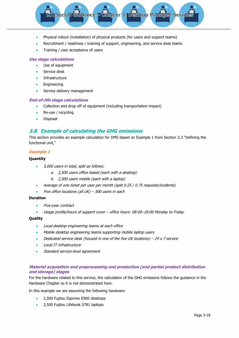
Page 3-18
Physical rollout (installation) of physical products (for users and support teams)
Recruitment / readiness / training of support, engineering, and service desk teams
Training / user acceptance of users
Use stage calculations
Use of equipment
Service desk
Infrastructure
Engineering
Service delivery management
End-of-life stage calculations
Collection and drop off of equipment (including transportation impact)
Re-use / recycling
Disposal
3.8 Example of calculating the GHG emissions This section provides an example calculation for DMS based on Example 1 from Section 3.3 “Defining the
functional unit,”
Example 1
Quantity
5,000 users in total, split as follows:
a. 2,500 users office based (each with a desktop)
b. 2,500 users mobile (each with a laptop)
Average of one ticket per user per month (split 0.25 / 0.75 requests/incidents)
Five office locations (all UK) – 500 users in each
Duration
Five-year contract
Usage profile/hours of support cover – office hours: 08:00–18:00 Monday to Friday
Quality
Local desktop engineering teams at each office
Mobile desktop engineering teams supporting mobile laptop users
Dedicated service desk (housed in one of the five UK locations) – 24 x 7 service
Local IT infrastructure
Standard service-level agreement
Material acquisition and preprocessing and production (and partial product distribution and storage) stages
For the hardware related to this service, the calculation of the GHG emissions follows the guidance in the
Hardware Chapter so it is not demonstrated here.
In this example we are assuming the following hardware:
2,500 Fujitsu Esprimo E900 desktops
2,500 Fujitsu Lifebook S781 laptops

Page 3-19
100 Hewlett Packard P3015 printers
25 Fujitsu TX300 servers
5 storage / backup arrays
25 switches
25 routers
As well as this, there is also the consideration for hot swap spares. In this example, we are assuming that
there are an additional 50 desktops, 50 laptops and 5 printers.
The calculation for these stages is based on guidance from the Hardware Chapter. The total emissions
were calculated as 450,000 kilograms (kg) CO2e, then as the example was for a five-year contract (the
time boundary and the service contract term are in this case assumed to be the same as the expected life
of the equipment), the figure can be amortized over the service contract term, resulting in 90,000 kg CO2e
per annum.
Product distribution and storage stage
Process a: Setting up of a project / program project rollout team
Setting up a project or program team relates to recruiting, training, and arming a team with relevant
knowledge and tools (e.g., project managers, engineers, and administration staff) so they are ready to
implement the rollout. In this example, the emissions relating to this are negligible and therefore ignored.
In some circumstances, for example on global DMS contracts, there may be requirements to fly people
around the world to recruit and train new members of staff, which would give some material value to
calculating/measuring the impact. For this example, it is assumed that the service provider will pull from a
pool of existing project people who are already trained, which implies that the GHG emissions from this
process are not significant.
Process b: Transportation of supported (physical) products from distribution center to customer location
In this example, the equipment is already in UK distribution centers, but transport needs to be arranged to
get to customer locations.
Criteria applied to the example scenario are as follows:
Distributed from: one location
Regional locations for delivery: 5
Number of delivery journeys required: 50
Average journey (km): 200
Type of vehicle: articulated truck between 3 and 33 metric tons
Loading: 45 percent (UK average)
Fuel: diesel
A calculation of the emissions for this example is shown below:
Total distance traveled = 10,000 km
Emission factor3 = 0.85763 kg CO2e per vehicle km
GHG emissions = 10,000 x 0.85763 = 8,576 kg CO2e
3 Guidelines to Defra / DECC’s GHG Conversion Factors for Company Reporting, October 2010, available at: http://archive.defra.gov.uk/environment/business/reporting/conversion-factors.htm

Page 3-20
The above calculation is based on factors provided by Defra / DECC, which are available on their website.
There are multiple options for transport, with different vehicle sizes and loadings. The unit of calculation in
this case is kilometers, although liters of fuel consumed may also be used as a method to calculate the
emissions.
Process c: Transportation of supported (physical) products to individual user location(s)
In some circumstances, there may be staging locations (for example a regional head office) within the
customer environment and a further step is required to deliver physical products to the individual locations.
In this example, the products have been delivered directly to the five office locations, so mobile users will
have to go to their nearest office to collect their laptop. Therefore the emissions in this example, for this
process are zero.
Process d: Physical rollout (installation) of physical products (for users and support teams)
In some scenarios this may involve significant travel time in visiting a large number of sites or users
(especially for global DMS requiring air travel by engineers). In this example, the users will be congregated
at the five key locations during rollout.
Assuming there are:
25 rollout engineers
rolling out on average 10 pieces of equipment per working day per engineer
with an average travel distance of 50 km per engineer per day,
it would take 21 elapsed days (rounded up) to install all the equipment, meaning 21 return journeys for
each engineer. This equates to 26,250 km traveled for all engineers combined (assume using diesel cars
with 1.7 – 2.0 liter engines).
A calculation of the emissions for this example is shown below:
Total distance traveled = 26,250 km
Emission factor* = 0.14689 kg CO2e per vehicle km
GHG emissions = 26,250 x 0.14689 = 3,856 kg CO2e
*Source: Defra / DECC’s GHG Conversion factors.
Processes e and f: Recruitment/readiness/training of support, engineering, and service desk teams and
training/user acceptance of users
In this example, it is assumed that all training and user acceptance takes place on site. Thus, it may be
assumed that there are no significant GHG emissions associated with these two processes. The reason for
this is that the training window is small (a week), thus the emissions for hosting the training (heating,
lighting, and bespoke training staff commute to the five customer locations) will be small compared with
the overall total.
In some circumstances, for example for global DMS, there may be requirements to fly people around the
world to recruit and train new members of staff (or to train users), which would make these processes
material, and hence necessary to calculate the impact.
Use stage
Use of end-user devices (by use profile)
The example estate is shown in Table 3.3 split by use profile. For each type of equipment, the power
consumption per unit is multiplied by the number of units, and then the use profile is applied. This gives a
total power consumption for all equipment in watts. This total is then multiplied by the “number of working

Page 3-21
days per annum” and the “usage per day” in hours used per year, then divided by 1,000 to give the yearly
energy consumption in kilowatt hours.
Finally the emission factor for the UK grid electricity is applied to give the number of kilograms of CO2e per
annum. For DMS covering multiple countries, there will, of course, be different grid electricity emission
factors depending on the country. A calculation of the emissions for this example is shown in Table 3.3.
Table 3.3. Example of emissions from usage of end-user devices
Use profile (power used and hours)1
Equipment type
Nr of units
Work-ing days p.a.
Max Idle Standby Off kWh p.a. (per unit)
kWh p.a.
(all) W hours W hours W hours W hours
Fujitsu
Esprimo E900 2,500 228 80.7 0.8 19.5 7.2 1.1 2.0 0.0 14.0 47.2 118,047
Fujitsu
Lifebook S781 2,500 228 33.0 0.8 13.0 7.2 2.0 2.0 0.0 14.0 28.3 70,680
HP Laserjet
P3015
(weekdays)
50 253 80.0 2.0 10.0 10.0 2.0 12.0 0.0 0.0 71.9 3,593
HP Laserjet
P3015
(weekend
+ public
holidays)
50 112 80.0 0.0 10.0 0.0 2.0 24.0 0.0 0.0 5.4 269
TOTAL 192,588
[kWh p.a. = kilowatt-hour per annum]
Electricity emission factor (UK grid power)2 = 0.54522 kg CO2e/kWh
Emissions per annum = 105,003 kg CO2e
Notes
1. The use-profile for desktops and laptops in the context of this worked example consists of on-mode = 8 hours per
working day, standby mode = 2 hours per working day for Monday to Friday use (accounting for a deduction for
employee annual leave). The on-mode for power consumption is further broken down to 90% idle, 10% maximum
power. Vendors usually provide (in the public domain on their corporate websites) power consumption information in
various usage modes to assist in the calculation process. The 90% / 10% split used in this example is determined by
the proposal of the European Methodology for the Ecodesign of Energy-related Products (MEErP) Product Cases
Report (2005) based on the MEEuP Methodology Report for the European Commission (2005), see
http://ec.europa.eu/growth/industry/sustainability/ecodesign/index_en.htm
For printers, there is no concept of annual leave and there is also a small power provision for printers being switched
on during weekends (in standby mode), as in this worked example they are available 24 x 7.
2. Defra / DECC’s GHG Conversion factors.
This summary is quite simplistic, assuming all equipment of the same type will have a similar usage profile.
However, if there are specific user types or specific roles for equipment, where the function means a
different use profile, then separate lines may be included.

Page 3-22
For example, if there were a subset of desktops that were used for processing complex mathematical
models, and in use 24 hours per day, 7 days per week, then a separate line may be included to
accommodate a higher utilization, hours usage per day, and working days per year for these devices. But
they should be treated as an exception rather than the rule and only if the difference in emissions is
significant enough to justify a separate inventory entry.
Service desk
The service desk calculation is similar to the equipment usage calculation. So a table similar to Table 3.3
can be applied specifically to the service desk if required. Alternatively, the equipment can be blended in as
a line in the use stage. In this scenario/example, the service desk is on the customer site and the desktops
for the service desk (25) are included in the figure for the Esprimo E900’s.
If a service desk has a highly different use profile, for example its desktops are utilized at 50 percent rather
than 30 percent, this can be included as a separate section or line under the “use of equipment” process.
Although there are no people-related emissions for the supported employees served by the DMS in relation
to facilities power/lighting/heating, the service desk, as a dedicated constituent part of the service should
account for both facilities power/lighting and any travel emissions. This also counts for the local deskside
engineering teams.
Proxy data on average CO2e emissions per office-based employee may be used if available. The preferred
alternative to using an average is to use the energy bill from the physical location that houses the support
staff. Then, either an allocation of heating/lighting is made for the percentage of total floor area taken up
by the service desk staff and dedicated service infrastructure, or by full time equivalent (FTE) (or seats) of
total FTE (or seats) in the building. There is no fixed method as to how this can be calculated, but it should
be considered, explored and either included or excluded from total emission calculations with appropriate
explanation.
Deskside services (engineering)
In this example, the DMS include mobile engineering support for laptop users, thus there is a requirement
to calculate this impact with regard to emissions.
For demonstrative purposes as to how this impact may be calculated, using the example.
Of the one ticket raised on average per month per user, 90 percent are resolved by the service
desk or local desktop engineering teams. Thus the remaining 10 percent of tickets that require a
mobile engineering visit will generate additional emissions.
For 2,500 laptop users, this means 250 visits per month.
Taking an average of 40 km travel distance for each engineering visit, in a diesel-fueled car (with
a 1.7 liter engine) this comes to 10,000 km per month or 120,000 km per year.
A calculation of the emissions for this example is shown below:
Total distance traveled = 120,000 km
Emission factor* = 0.14689 kg CO2e per vehicle km
GHG emissions = 120,000 x 0.14689 = 17,627 kg CO2e
*Source: Defra / DECC’s GHG Conversion factors.
Deskside engineering teams will also need to have the emissions of their facilities included in the
calculation (much like the service desk).
Proxy data on average CO2e emissions per office-based employee may be used if available. The
preferred alternative to using an average is to use the energy bill from a physical location which houses the
support staff. Then, either an allocation of heating/lighting is made for the percentage of total floor

Page 3-23
area taken up by the service desk staff and dedicated service infrastructure, or by FTE (or seats) of
total FTE (or seats) in the building. There is no fixed method as to how this can be calculated, but it
should be considered and either included or excluded from total emission calculations with an
appropriate explanation.
End-user infrastructure
This may include any infrastructure that supports the end-users, not including the end-user devices, which
are covered under their own section.
In this example, end-user infrastructure covers a number of servers, disk stores, backup devices, and
network equipment. Servers cover such functions as mail, print, application, and service management
toolsets.
A table similar to Table 3.3 can be generated for the end-user devices. An example is shown in Table 3.4.
Table 3.4. Example of emissions from usage of end-user infrastructure
Equip-
ment type
No. of
units
Power per unit (W)
Avge
% utili-
zation
Total power
(W)
Usage per day
(hours)
Working days per
year
Total energy
per annum (kWh)
Alloca-tion
Adjusted energy
per annum (kWh)
Servers 25 560 60% 8,400 24 365.25 73,634 90% 66,271
Storage/
backup
array
5 4,000 25% 5,000 24 365.25 43,830 100% 43,830
Switches 25 200 25% 1,250 24 365.25 10,958 100% 10,958
Routers 25 220 25% 1,375 24 365.25 12,053 100% 12,053
TOTAL 16,025 140,475 133,112
Electricity emission factor (UK grid power)1 = 0.54522 kg CO2e/kWh
Emissions per annum = 72,575 kg CO2e
Notes: 1. Defra / DECC’s GHG Conversion factors.
Average utilization of total power is used in this worked example. Methods such as directly measuring the
power consumption can be used to derive the power consumption if power monitors can be included on a
server rack, for instance. Or, they may be measured for a set time frame, with the results extrapolated for
the relevant time period (e.g., one year).
Allocation may need to be considered in this section, especially if infrastructure is shared among different
organizations. In this example it is mostly ring fenced, but this organization shares its service desk toolset
(and server) with other organizations. Thus there is an adjustment using an allocation factor of 90 percent.
Section 3.5 “Allocation” goes into greater detail as to methods of how this may be applied (e.g., through
consumption of resources, or financial). In this case, the allocation method is based on usage, (i.e., total
number of tickets logged among the organizations). Since 90 percent of the tickets come through the host
organization, a 90 percent allocation factor is used.

Page 3-24
End-of-life stage
For the end-of-life calculations, please refer to the Hardware Chapter.
In some circumstances, collection of legacy equipment takes place at the same time as the deployment of
the new infrastructure, so there will be an overlap of activity. In this case, the emissions of the transport
should be allocated among the products.
Distribution and storage stages and end-of-life stages
Examples of the transportation of equipment and the movement of engineers have been covered
previously and the same approach can be applied here.
Collation of results
The final stage is to collate and report the overall GHG emissions of the service, (refer to the Introduction
Chapter). The key elements are summarized in Table 3.5:
Table 3.5. Example of summary of emissions by stage
Stage Process Element Electricity use
(kWh per year)
GHG emissions
(kg CO2e per year)
Material acquisition
and production
Hardware 90,000
Distribution a Project set-up -
Distribution b Delivery of hardware
to customer site
8,576
Distribution c Delivery of hardware
to individual user
-
Distribution d Installation 3,856
Distribution e & f Training, UAT -
Use End-user devices 192,588 105,003
Use Service desk -
Use Deskside services 17,627
Use Infrastructure 133,112 72,575
End-of-life -
TOTAL 325,700 297,637
For this example, where desktop managed services were provided to a client company over a five-year
period, for 5,000 users, it was found that providing the DMS resulted in 297,637 kg CO2e per year.
Alternatively, this can be expressed as 59.5 kg CO2e per user per year.

ICT Sector Guidance built on the
GHG Protocol Product Life Cycle Accounting and Reporting Standard
Chapter 4: Guide for assessing GHG emissions of
Cloud Computing and Data Center Services
July 2017
This Guidance has been reviewed for conformance with the GHG Protocol Product Standard.

Page 4-2
Contents
Chapter 4: Guide for assessing GHG emissions of Cloud Computing and Data Center Services ................ 4-1 4.1 Introduction ....................................................................................................................... 4-5
4.1.1 What is in this chapter ..................................................................................................... 4-5 4.1.2 How to use this guidance ................................................................................................. 4-5 4.1.3 The audience for this chapter ........................................................................................... 4-5 4.1.4 Examples: When to use and when not to use this chapter .................................................. 4-5 4.1.5 Rationale of this chapter .................................................................................................. 4-6 4.1.6 Definitions for cloud and data center services .................................................................... 4-6
4.2 Overview of method ............................................................................................................ 4-8 4.2.1 Cloud services and data centers ....................................................................................... 4-8 4.2.2 Capturing all emissions of the data center ......................................................................... 4-9 4.2.3 Fixed and variable emissions ............................................................................................ 4-9 4.2.4 Allocation process ......................................................................................................... 4-10 4.2.5 Calculation process ........................................................................................................ 4-11
4.3 Functional unit .................................................................................................................. 4-11 4.3.1 Functional unit: cloud services........................................................................................ 4-11 4.3.2 Functional unit: data center services ............................................................................... 4-12
4.4 Boundary setting ............................................................................................................... 4-13 4.4.1 Defining boundaries ...................................................................................................... 4-13 4.4.2 Attributable processes ................................................................................................... 4-13 4.4.3 Non-attributable processes ............................................................................................ 4-14 4.4.4 Temporal considerations – amortization of embodied emissions ........................................ 4-14
4.5 Data collection and data quality ......................................................................................... 4-14 4.6 Allocation ......................................................................................................................... 4-18
4.6.1 Allocating data center emissions ..................................................................................... 4-18 4.6.2 Allocating IT equipment to cloud services........................................................................ 4-22 4.6.3 Allocating IT equipment to data center services ............................................................... 4-23 4.6.4 Allocating network emissions.......................................................................................... 4-23 4.6.5 Allocating end-user device emissions .............................................................................. 4-24
4.7 Calculating inventory results .............................................................................................. 4-24 4.7.1 Overview of calculation methodology for cloud services ................................................... 4-24 4.7.2 Screening assessment ................................................................................................... 4-25 4.7.3 Calculating data center emissions ................................................................................... 4-25 4.7.4 Calculating network emissions ........................................................................................ 4-26 4.7.5 Calculating end-user device use ..................................................................................... 4-30 4.7.6 Electricity emission factors ............................................................................................. 4-30 4.7.7 Calculating embodied emissions ..................................................................................... 4-30 4.7.8 Case study of cloud service ............................................................................................ 4-33 4.7.9 Example calculations for data center services .................................................................. 4-34

Page 4-3
Tables
Table 4.1. Examples of functional units for cloud services ....................................... 4-12 Table 4.2. Conversion of square feet to kilowatts .................................................. 4-20 Table 4.3. Relative contributions of different aspects of cloud and
data center services ............................................................................ 4-25 Table 4.4. Application of alternative methods for calculating data center emissions ... 4-26 Table 4.5. Summary of studies estimating the energy intensity of the internet .......... 4-27 Table 4.6. Examples of Life cycle stage ratios for business-to-consumer
and business-to-business ICT hardware ................................................ 4-31 Table 4.7. Hosting provider site inventory ............................................................ 4-35 Table 4.8. Company site inventory ...................................................................... 4-36 Table 4.9. Data center asset owner inventory – single site,
allocation by provisioned capacity ........................................................ 4-37 Table 4.10. Service application equipment inventory – all IT equipment
owned by a single service application across multiple sites .................... 4-37
Figures
Figure 4.1. Data center layers ............................................................................. 4-10 Figure 4.2. Allocation steps ................................................................................ 4-10 Figure 4.3. Generic scope and boundary for equipment used by cloud services ......... 4-13 Figure 4.4. Flow chart of energy use throughout a site ........................................... 4-16 Figure 4.5. Example data center physical layout .................................................... 4-17 Figure 4.6. Allocation steps ................................................................................ 4-19 Figure 4.7. Fixed line and mobile network energy intensity ..................................... 4-29
Page 4-4
Executive Summary: Cloud and data center services
Cloud and data center services are becoming increasingly commonplace, replacing IT services that use
corporate in-house dedicated computing infrastructures. Cloud computing provides application hosting, often
using shared resources, with convenient, on-demand, ubiquitous, remote access via the internet. Cloud
services are typically provided remotely by a third party, but may also be provided on premise. Data center
services allow companies to meet their computing requirements through a mix of leasing options more
efficiently in terms of energy and more cost effectively than using their own dedicated facilities. These
advantages have driven rapid growth in cloud computing services and internet usage, as well as exponential
growth in data centers. This growth has raised concern over the energy consumption of networks and data
centers.
This chapter provides guidance for calculating the greenhouse gas (GHG) emissions related to cloud and
data center services, allowing practitioners to assess and study the GHG impact of these services. If detailed
measurements are not available, a key question is how to allocate the GHG emissions of a data center to its
various services and clients. This chapter gives guidance, and provides a number of different allocation
methods (dependent on the type of data center, the type of service, and the type of metering and
information available at the data center).
The GHG emissions of cloud services relate to three areas that make up the delivery of the service:
emissions of the data center, the network, and the end user devices (such as PCs, laptops, tablets, and
phones). This chapter describes how to calculate the emissions of these separate elements. Other chapters
in this ICT Sector Guidance provide further details: the Hardware Chapter for emissions of ICT hardware;
the Telecommunications Network Services Chapter for emissions of networks; and the Software Chapter for
the emissions of software.
This chapter concludes with a case study for assessing a cloud service and some examples for calculating
emissions of data center services (illustrating the different allocation methodologies that may be used).

Page 4-5
4.1 Introduction
4.1.1 What is in this chapter This chapter forms part of the ICT Sector Guidance, built on the Greenhouse Gas Protocol Product
Life Cycle Accounting and Reporting Standard (referred to as the Product Standard) and covers
cloud and data center services
It provides guidance and accounting methods for the calculation of GHG emissions related to cloud
and data center services
The chapter provides guidance on the following key items:
Establishing the scope of a product inventory
Defining the functional unit
Boundary setting
Allocation
Collecting data and assessing data quality
Calculating inventory results and GHG emissions
A case study for assessing cloud services
Examples of calculating emissions of data center services
4.1.2 How to use this guidance
The purpose of this Sector Guidance is to provide additional guidance to practitioners who are implementing
the Product Standard for ICT products (including ICT services). This Sector Guidance follows a life cycle
approach to the assessment of ICT products (including services). The ICT Sector Guidance is a supplement
to the Product Standard, and thus assumes that the reader is familiar with the principles and content of the
Product Standard. The ICT Sector Guidance is divided into chapters, with general guidance provided in the
Introduction Chapter, and specific guidance in each of the subject chapters. The chapters cover the
following subjects: Telecommunications Network Services; Desktop Managed Services; Cloud and Data
Center Services; Hardware; and Software.
This chapter should be used in conjunction with the Introduction Chapter and with the Product Standard.
4.1.3 The audience for this chapter
Potential users of this chapter include:
Suppliers of cloud and data center services, who require standard terminology, guidance, and
accounting methods to calculate the GHG emissions of the services they provide. This accounting
may be required by their customers and potential customers. It can also be used to understand
what are the major sources of GHG emissions from cloud and data center services, and how the
suppliers may reduce emissions from the services that they provide.
Users of cloud and data center services, who are interested in understanding the amount of
GHG emissions from the services they are using, and where improvements and efficiencies may be
made.
Organizations, which are interested in understanding the GHG emissions of cloud and data center
services, especially in relation to more traditional ways of delivering the same services.
4.1.4 Examples: When to use and when not to use this chapter
This guidance is for accounting of GHG emissions from cloud and data center services. Examples of where it
may be used are:
For assessing the GHG emissions of a cloud service provided from one or more data centers

Page 4-6
For assessing the GHG emissions associated with the use of all or part of a data center (e.g., where
all or part of a data center is leased from a data center provider).
For comparing the GHG emissions of a cloud service with those from an equivalent non-cloud
service. (For this type of use, it is important to apply the same boundary conditions to both cases,
and it is recommended to carry out an uncertainty analysis to understand the comparison of the
results).
This guidance for cloud and data center services should not be used:
For comparison of similar cloud or data center services from different providers without additional
specifications to ensure a valid comparison.
4.1.5 Rationale of this chapter
A range of business and consumer applications are increasingly provided from cloud architecture, for
example:
E-mail, calendar, document, and other business applications
Consumer photo, video, music, and other data storage applications
Search, social networking, and database applications
Application hosting
This chapter provides guidance on how to quantify the energy and GHG emissions associated with the
delivery of these services. The guidance is written from the perspective of a cloud services user and aims to
provide standard and repeatable methods to facilitate a better understanding of the energy and GHG
impacts of alternative ICT service delivery solutions.
4.1.6 Definitions for cloud and data center services
Cloud computing is a model for enabling ubiquitous, convenient, on-demand network access to a shared
pool of configurable computing resources (e.g., networks, servers, storage, applications, and services) that
can be rapidly provisioned and released with minimal management effort or service provider interaction.1 As
such, it can yield significant efficiencies in providing ICT services and can reduce GHG emissions based on
how the service is configured and deployed.2 Colocation data center services, which differ from cloud
services in that the user has control of the specification and management of the host IT devices, if properly
operated, may also yield life cycle efficiencies compared with traditional in-house IT hosting.
This guidance allows cloud and data center service providers and customers to measure and report the GHG
emissions from their services in a consistent manner and make informed choices to reduce GHG emissions.
For the purposes of this guidance, cloud services are services provided to computers and other end-user
devices as a utility over a network, using shared infrastructure that includes data centers, hardware,
software, and other infrastructure. This guidance adopts the standard definitions and taxonomy for cloud
services developed by NIST1 (National Institute of Standards and Technology), listed according to
decreasing levels of operational control by the user:
1 P. Mell and T. Grance, “The NIST Definition of Cloud Computing,” NIST Special Publication 800-145, (National Institute of Standards and Technology, September 2011).
2 National Resources Defense Council and WSP Environment & Energy, “The Carbon Emissions of Server Computing for Small-to-Medium-Sized Organizations,” October 2012.
https://www.wspgroup.com/Globaln/USA/Environmental/Sustainability/Documents/NRDC-WSP_Cloud_Computing.pdf

Page 4-7
Infrastructure as a Service (IaaS): The capability provided to the consumer is to provision
processing, storage, networks, and other fundamental computing resources where the consumer is
able to deploy and run arbitrary software, which can include operating systems and applications.
The consumer does not manage or control the underlying cloud infrastructure but has control over
operating systems, storage, and deployed applications; and possibly limited control of select
networking components (e.g., host firewalls).
Platform as a Service (PaaS): The capability provided to the consumer is to deploy onto the
cloud infrastructure consumer-created or acquired applications created using programming
languages, libraries, services, and tools supported by the provider. The consumer does not manage
or control the underlying cloud infrastructure including network, servers, operating systems, or
storage, but has control over the deployed applications and possibly configuration settings for the
application-hosting environment.
Software as a Service (SaaS): The capability provided to the consumer is to use the provider’s
applications running on a cloud infrastructure. The applications are accessible from various client
devices through either a thin client interface, such as a web browser (e.g., web-based email), or a
program interface. The consumer does not manage or control the underlying cloud infrastructure
including network, servers, operating systems, storage, or even individual application capabilities,
with the possible exception of limited user-specific application configuration settings.
Data center services are defined as “wholesale” and “colocation” services, in which the service provider
leases space in a facility and provides mechanical, electrical, and other operational services to users (i.e.,
lessees). The lessee has full control of specification and management of the IT devices hosting the services.
Wholesale leases: the lessee may lease the entire data center, pay utility bills, and
operate/maintain the physical infrastructure. Alternatively, the lessee may lease the entire site, and
rely on the owner for operation and maintenance of the critical environment infrastructure
(electrical, mechanical, and other critical infrastructure) and payment of utility bills.
Colocation leases: the owner operates and maintains all critical data center infrastructure;
however, in some cases the owner operates and maintains ICT infrastructure and leases servers as
physical hosts. Alternatively, an area of the data center with basic power/cooling/security is
provided and the lessee operates all ICT equipment.
The underlying energy-using infrastructure used by cloud and data center services includes:
Hardware: servers, switches, and routers that store and transmit information
Software: which controls and commands the hardware to process information and thus
determines how much power is consumed
Data centers: which house servers and other hardware devices for storing and fulfilling services
and provide critical systems and other ancillary equipment
Network: which includes wired or wireless infrastructure for transmitting information from cloud
infrastructure to end users
End-user (or “client”) devices: including computers, smart phones, and other devices used for
accessing cloud services
The chapter draws from the methods outlined in the Telecommunication Network Services and Hardware
Chapters of this ICT Sector Guidance, which prescribe the methods for calculating the GHG impacts of the
various component parts of the infrastructure that support a cloud service.

Page 4-8
4.2 Overview of method This section provides an overview of the approach for calculating the GHG emissions from cloud and data
center services. This overview is expanded throughout the rest of this chapter.
4.2.1 Cloud services and data centers
Relationship between cloud services and data centers
Cloud services include use of:
Data centers
Networks
End user devices
Thus calculating the emissions from cloud services involves calculating the emissions from the data center
and allocating them to a specific service.
Data center definition
The guidance in this chapter is applicable to different types of data centers, thus the definition adopted is
deliberately broad.
A “data center” is a physical location dedicated to hosting ICT infrastructure:
A data center may be a mixed-use or a dedicated facility.
Data centers may be of varying tiers or form factors; that is, providing different levels of security,
redundancy, etc.
Data centers may host ICT infrastructure for internal use or provide services for external customers,
with a diverse set of business applications or usage at any physical location.
Data centers may be used for testing or production of applications, services, platforms or clouds.
Data centers may vary in size in terms of total useable capacity for ICT equipment.
Data center overhead
It is well understood within the industry that a data center uses more input energy than it delivers to the IT
equipment. The resulting energy overhead is because of the data center mechanical and electrical (M&E)
infrastructure, and is commonly measured with the metric power usage effectiveness (PUE),3 which
represents the ratio between the total facility power and the IT equipment power.
This energy overhead (or non-IT energy) includes the energy used by cooling systems, and power-delivery
components such as the uninterruptible power supply (UPS), switch gear, generators, and batteries.
Data center capacity
It is common for data center “capacity” to be based either on provisioned circuit power (kilowatts [kW]) or
on physical floor area (square meters or square feet). The data center lease will provide a specified power
or floor area, which may then be divided further to a rack, cage, or server level. The data center will
typically be designed to a specification of maximum power provision, with the infrastructure equipment and
cooling capability designed for this maximum power. It is, therefore, appropriate to use the data center
3 The Power Usage Effectiveness (PUE) ratio was developed as a key data center efficiency metric by The Green Grid Consortium, “The Green Grid Data Center Power Efficiency Metrics: PUE and DCiE,” White Paper 6, (The Green Grid, October 23, 2007).
http://www.thegreengrid.org/Global/Content/white-papers/The-Green-Grid-Data-Center-Power-Efficiency-Metrics-PUE-and-DCiE.

Page 4-9
capacity to allocate overhead. The data center “capacity” is measured in terms of kilowatts (although it can
also be derived from floor area or from numbers of racks). In this chapter the term “provisioned capacity”
refers to the circuit power (or floor area) allocated to the data center, to an individual customer, service, or
set of IT equipment.
4.2.2 Capturing all emissions of the data center
A key aspect of calculating emissions from data center services and cloud services is the allocation of the
data center emissions to the individual services (see Section 4.6 “Allocation”). As relates to the accounting
principle of completeness4: all data center emissions should be allocated to the services that the data center
delivers. This can be summarized as:
Allocate all of the emissions
The first step is to allocate the entire GHG emissions of the data center to the services it delivers.
This includes both the utility energy supply and the embodied emissions in the devices.
All IT devices should be allocated to a service
The second step is to allocate all IT devices in the data center to a delivered service. If a device, such as
shared network, shared storage, or monitoring systems, supports more than one service, divide its allocation
across the other devices using a consistent allocation per physical device, logical device, or service unit. IT
equipment that manages workloads for a service or that serves as reserve capacity for a service, should also
be allocated to that service and its users.
4.2.3 Fixed and variable emissions
A key consideration in defining and implementing an allocation mechanism is to separate the data center’s
overhead emissions into fixed and variable categories.
The data center’s fixed emissions do not vary with the degree of service consumption or the IT electrical
load. They include the embodied emissions of the data center, the fixed part of the data center energy
overhead, and the fixed energy consumption of the IT devices.
A substantial part of the energy overhead does not vary with the data center’s IT electrical load. This mix of
fixed and variable overheads is the cause of the commonly observed efficiency decrease (or PUE increase)
with decreasing IT electrical load. This is also true at the level of the IT device, (for example, servers may
use over 60 percent of their peak workload electrical power at zero or low load,5 although chip and server
manufacturers are now working at reducing this system idle power).
The difficulty of determining the precise mix of fixed and variable infrastructure overheads for a site has an
important implication for measurement and reporting. The inherent error margin in scaling an IT load to the
allocated utility energy tends to negate any increase in accuracy obtained through device-level metering.
Other estimation methods are likely to be of equivalent overall accuracy and operators are not expected to
install IT device-level power metering simply to report emissions.
As far as reasonable, based on the available data, the selected allocation method should seek to separate
the fixed and variable emissions of the site. The intent is to allocate the fixed emissions based on the
provisioned capacity and variable emissions based on the energy consumption of each platform, customer,
or device.
4 See Chapter 4 of the Product Standard. 5 D. Meisner, B.T. Gold, and T.F. Wenisch, “PowerNap: Eliminating Server Idle Power,” ASPLOS XIV: Proceedings of the 14th International Conference on Architectural Support for Programming Languages and Operating Systems, 2009, pp. 205–16.

Page 4-10
4.2.4 Allocation process
A data center is like an onion with multiple layers (Figure 4.1). At each layer an allocation is potentially
necessary.
Figure 4.1. Data center layers
The allocation steps are summarized in Figure 4.2.
Figure 4.2. Allocation steps
Fixed EmissionsAllocated kW
Variable Emissions
Drawn kWh
Fixed EmissionsAllocated Capacity
Variable EmissionsUtilised Capacity
Virtual Machine
Other Virtual Machines
Service
Other Services
User
Other Users
Data Center IT Devices Virtual Machines Services Users
Allocate the data center emissions:
Allocate fixed emissions to IT devices based on the provisioned capacity for the IT device or
group of devices.
Allocate variable emissions to IT devices based on the energy consumption of the IT device
or group of devices.
If virtual machines are in use, allocate IT device emissions to virtual machines, for example:
Allocate the IT device fixed emissions (based on idle power) to virtual machines based on the
fraction of machine capacity allocated to the virtual machine or based on a simple fixed
emissions to total virtual machines approach.

Page 4-11
Allocate the IT device variable emissions (based on actual power minus idle power) to virtual
machines based on a suitable proxy for the work such as central processing unit (CPU) load.
Allocate IT device emissions (or virtual machine emissions) to services.
If a service is used by more than one user, allocate the service emissions to the individual users.
The allocation methods chosen for each step will depend partly on the data available, and on the type of
service being delivered. The allocation methods are all physical allocation methods (see Chapter 9 of the
Product Standard). The time period for the allocation should align with the time period for reporting the data
center emissions, typically this would be measured on an annual basis.
Section 4.6 “Allocation,” provides more detailed guidance on the different allocation methods.
4.2.5 Calculation process
The calculation process is described further in Section 4.7 “Calculating inventory results.” The process
involves calculating and summing the data center emissions, network emissions, and end-user device
emissions, and then allocating these to a service.
4.3 Functional unit The functional unit should include a definition of the following three parameters:
Quantity of the service: this is the defining parameter for the service and typically equates to how the
service is sold. Some typical examples are:
Number of users, mailboxes supported
Size of storage capacity (e.g., gigabytes) provided
Quantity of computing capability provided (e.g., number of minutes, or number and type of servers)
Duration of the service: typically expressed in terms of years. Some examples are:
Per year, month, day, hour, or minute
For the contract duration (one or multiple years)
Quality of the service: this should describe the relevant service levels, where they exist, as these may
have a significant impact on the resources required to provide the service, in terms of recovery/availability.
4.3.1 Functional unit: cloud services
Cloud services are procured in different ways, for example: on a per-user basis or by storage capacity (e.g.,
gigabytes of data stored), both measured over a period of time (e.g., per day or per year). These are useful
starting points for defining the functional unit of cloud services. Where use profiles vary significantly for
cloud services, “transactions” may better reflect the key indicator – that is, the number of application
programming interfaces (API) and web requests processed by the platform over a period of time.
The following functional units may be used when analyzing cloud services, and should be selected based on
the characteristics of the cloud service as shown in Table 4.1:

Page 4-12
Table 4.1. Examples of functional units for cloud services
Functional unit Example cloud services Characteristics
Per user (or user
group)
E-mail, calendar, document
and other business
applications
High data storage
requirements and high user
access
Per unit of storage
capacity
Consumer photo, video, music,
and other data storage
applications
High data storage
requirements and low user
access
Per transaction Search, social networking, and
database applications
Low data storage
requirements; high user access
Servers hosting cloud services do not follow a linear scale as users increase. To account for this, when
undertaking analysis on a per-user basis, it may be necessary to aggregate users into groups to understand
the efficiencies of scale provided by cloud services. These user groups may be defined by the number of
users or by the terms of a license or service level agreement.
Transaction-based analysis enables more accurate comparison of alternative cloud platforms. A transaction
can be defined as a WebAPI (i.e., a web request/response), for example. However, because of the diversity
and complexity of transactions and the lack of a standardized methodology to separate each type of
transaction, one can assume that all transactions for a given service require the same amount of energy
load on IT hardware, based on typical packet size and type of transaction.
The functional unit should define the level and quality of service, especially in cases where the basis for
normalization is complex and could be misleading. For instance, instead of simply defining the functional unit
as an API, additional descriptive information should clarify what an API means for a given type of service
and the range of physical resource demands for various types of APIs.
As a further example, even for a service such as email, a range of parameters will legitimately affect the
energy consumption of the delivered user service, including:
1. The size of the mailstore (in both messages and total data volume)
2. The number of messages sent and received in each unit time
3. The extent of filtering, virus scanning etc., carried out on each routed message
4. Whether the messages are viewed as web mail or downloaded by a client application using a
protocol such as POP or IMAP, or both
5. The level of resilience and availability of the email infrastructure, for example, redundant front-end
servers and duplicate storage of the mailstore(s) across multiple data centers
6. The additional functionality provided, for example, calendaring
7. The physical location (geographic region and jurisdiction) in which the data is held and processed
4.3.2 Functional unit: data center services
For data center services, the functional unit should clearly describe the kind of lease (wholesale or
colocation) and fully define the scope of the service in terms of quantity and time period, and any particular
service level agreements that are part of the service.

Page 4-13
4.4 Boundary setting
4.4.1 Defining boundaries
Cloud and data center services create emissions in three main places:
Data centers: switches, routers, and servers/storage devices used for receiving, sending, and
storing data and the associated critical systems, facilities, and utilities
Network: routers, switches, cables, and other equipment associated with the transfer of data
between the data center and end user
End-user devices: PCs, laptops, tablets, phones, or other devices used to access cloud services
The generic boundaries for aspects of infrastructure that support cloud service delivery are shown in Figure
4.3. Depending on the nature of specific cloud applications, it may not be necessary to include certain
aspects.
Figure 4.3. Generic scope and boundary for equipment used by cloud services
4.4.2 Attributable processes
Required processes directly attributable to the GHG impact of cloud and data center services are:
Hosting and fulfillment of the cloud applications – including servers, storage devices, other IT
equipment (e.g. networking devices, equipment that manages workloads for a service, or
equipment that serves as reserve capacity), critical systems, and associated data center facilities
including HVAC systems required for server cooling
Internet transfer
User access
Energy, water, refrigerants, fire suppression gases, and other materials consumed by the above
processes throughout their life cycle

Page 4-14
4.4.3 Non-attributable processes
Optional processes that are not attributable to the GHG impact of cloud and data center services are:
Energy consumed during software development
Material and energy flows from production of capital equipment, transportation vehicles, buildings
and their energy use not directly related to equipment for hosting and fulfillment of the cloud
service and associated equipment
Maintenance of capital equipment
4.4.4 Temporal considerations – amortization of embodied emissions
The embodied emissions of the equipment should be amortized over the expected in-use lifetime of the
equipment. How to calculate the embodied emissions is explained in Section 4.7.7 “Calculating embodied
emissions” and further in the Hardware Chapter. The embodied emissions are divided by the lifetime in
years to give the annual amortized embodied emissions. The lifetime will vary depending on the equipment
type and on the renewal policy of the data center. This may also vary based on the type of technology used.
Examples of lifetimes for infrastructure and IT equipment are:
25 years: main MV (medium voltage) transformers, some electrical switchgear
15-20 years: chillers, cooling towers, main-chilled water pipework, backup generators, low-voltage
distribution cabling and switchgear, AHU (air handling unit)
10-15 Years: UPS (uninterruptible power supply), data hall electrical PDU (power distribution
unit), CRAC (computer room air conditioning) units
<10 Years: elements closely coupled to IT such as in-row cooling units, rack exit door coolers,
smart power strips, etc.
18 months-5 years: IT equipment
It is usual practice to align the amortization of the embodied emissions with the assumptions used for
amortization of capital costs for financial accounting purposes. Assumptions used for amortizing equipment
should be clearly stated in supporting documentation.
4.5 Data collection and data quality As required by the Product Standard, data shall be collected for all processes included in the inventory
boundary, which includes all the attributable processes. Primary data shall be collected for processes under
the ownership or control of the reporting company.
Depending on the service being assessed and the allocation method being used, the following data may be
required:
Users: use profiles and number of users at any given period of time
Licensing or service level agreements: the units of service defined, for example, the number of
users for a specified period of time
Transactions: for example, measured Iops (input-output operations per second) or
WebAPIs/requests processed by the platform, over a specified time period
Data centers: number and location
Server count: number of servers provisioned to host and fulfill the cloud application and data
storage requirements. This includes redundancy for business continuity and disaster recovery
Network link equipment count: number of in-data-center routers and switches required to fulfill
WebAPI requests and process web transactions. This includes redundancy for business continuity
and disaster recovery

Page 4-15
Device utilization: computational load that a device is managing relative to the specified peak
load
Power consumption per type of IT hardware: calculated energy consumed by a server at a
given rate of device utilization and estimated power for networking and storage equipment
Data center power usage effectiveness (PUE): defined as the ratio of overall power drawn by
the data center facility, to the power delivered to the IT hardware. This is a data-center-specific
metric and accounts for energy consumption of active cooling, power conditioning, lighting, and
other critical data center infrastructure.
Emission factors – equipment: factors for the embodied emissions of relevant IT equipment,
ideally obtained from equipment manufacturers. See also the Hardware Chapter for methods of
calculating and estimating these.
Emission factors – electricity: the emission factor for the electricity used should be appropriate
for the region where the electricity is consumed. Electricity grid emission factors are published
nationally, and in some cases, regionally. Electricity grid emission factors should include the full life
cycle of the energy source (i.e., include emissions from extraction and transportation of the fuel, as
well as generation and transmission of electricity).
If primary data is not available, secondary data and/or assumptions may be developed for processes that
are not under the ownership or control of the reporting company. These might include:
Internet transfer: secondary data on access and core network usage (see Section 4.7.4
“Calculating network emissions,” and also the Telecommunications Network Services Chapter for
more details)
Embodied emissions for hardware: estimates of embodied emissions per server
The use of all primary and secondary data shall be clearly documented and communicated with the results
of the GHG inventory, including commentary on:
Technological representativeness: the degree to which the data reflects the actual equipment
and infrastructure used to support the cloud service
Geographical representativeness: the degree to which the data reflects the actual geographic
location of the equipment used to host and fulfill services (e.g., region or site)
Temporal representativeness: the time period to which the data refers
Completeness: the degree to which the data is statistically representative of the cloud services
Reliability: the degree to which the sources, data collection methods, and verification procedures
used to obtain the data are dependable
Additionally, the Product Standard requires companies to carry out a data quality assessment (see the
Introduction Chapter and section 8.3.7 of the Product Standard).
Data center energy data
Energy (in kilowatt hours [kWh]) used by a data center is a key item to be measured. Figure 4.4 identifies
typical measurement points within a data center.

Page 4-16
Figure 4.4. Flow chart of energy use throughout a site
Measurement of kilowatt hours at both points M1 (utility) and M4 (IT equipment) allows for the calculation
of the PUE for the data center. If possible, to improve the accuracy of tracking on a per rack or device level,
the data center operator may also track the remaining measurement points. Note that this is a large
undertaking, particularly in older sites with a variety of monitoring systems. Retrofitting an existing data
center may require a large investment in instrumentation, as well as data acquisition and reporting software.
Hardware and software-based equipment power monitoring techniques (M7 and M8) are evolving rapidly
and becoming more cost effective. Deployment of software monitoring systems, where the hardware
systems have the APIs needed to provide the data to the software system, can efficiently track IT energy
use by customer account.
Data center capacity
Data center “capacity” is commonly sold based either on provisioned circuit power (kilowatts) or on physical
floor area provided (square meters or square feet).
By way of comparison, in commercial buildings, the floor area (in square feet [ft2] or square meters [m2]) is
the basic unit of capacity management, and demand for additional floor area drives takedown of additional
capacity. Key metrics for commercial buildings are cost per floor area and floor area per person, as well as a
variety of other metrics depending on the use of the building.
In the data center industry, the common unit for measuring capacity is kilowatts. Secondary units, such as
racks or floor area, are also used throughout the industry, but are easily converted back to kilowatts. The
industry is currently gravitating toward using kilowatts as the basis for capacity management, and for ease
of calculation, this guidance recommends conversion of other units to kilowatts for analysis of each site.
A data center is typically designed to a specification of maximum power provision, with the infrastructure
equipment and cooling capability designed for this maximum power. Thus, it is appropriate to use the data
center capacity to allocate the fixed emissions overhead.

Page 4-17
For example, if a data center is designed to provide 10,000 kW of capacity for ICT equipment, the fixed
emissions for a service can be allocated based on its share of the data center’s total capacity. This share
should include a portion of any unused data center capacity, allocated pro rata.
Data center capacity example
A typical physical layout for a data center is shown in Figure 4.5 to provide a better understanding of data
center capacity and its allocation to specific IT devices.
Figure 4.5. Example data center physical layout
In a typical colocation data center, IT equipment is hosted in a physical room, or multiple rooms, with
adequate power and cooling to support reliable site operations. The floor plan in Figure 4.5 is a data center
with one room (Colo1) for IT equipment, served by electrical and mechanical equipment, with 1.98MW of
useable capacity, backed by a UPS with nominal capacity at output to the IT equipment room of 2.2MW.
It is recommended to track capacity within each IT equipment room (Colo1) and determine the capacity of
power provisioned for each rack in the room. A typical data center may have a variety of rack types with
different numbers of circuits deployed to each, and thus each rack may be tracked individually.
Key for Figure 4.5:
Colo: Colocation
CRAC: Computer Room Air Conditioning
PDU: Power Distribution Unit
RPP: Remote Power Panel

Page 4-18
Identifying IT equipment ownership – IT asset management inventory
IT asset management systems are used by data center owners to track ownership of equipment hosted in
their data centers. IT asset management inventories are required for business reasons, such as property tax
reporting, and are subject to quality controls. Inventories usually include all IT equipment installed,
particularly all assets plugged into power sources at the site, specifying the ownership by business division
or owning organization, purchase information, and application/service usage.
For a data center provider selling wholesale data center space (i.e., space provided with power, lighting,
security, etc.) the wholesale provider tracks the total kilowatts of useable capacity, metered or unmetered,
for each customer, while the lessee maintains an inventory of its assets.
To allocate emissions, the asset inventory data may be matched to installed racks or circuits.
4.6 Allocation This section describes the allocation of emissions from data centers, networks, and end user devices.
4.6.1 Allocating data center emissions
Choice of allocation method
Methods used to allocate data center emissions vary in difficulty of implementation or applicability to the
business need, depending on the type and complexity of the data center, what data is easily available and
the type of service being assessed. Each company should choose a method that meets its business needs.
The allocation methodologies in this section are best practices that may or may not be applicable to the
needs of a particular company, and are consistent with the allowable options in the Product Standard.
Each company should select a method based on cost or expediency; establishing and adhering to a practice
for the entire data center GHG inventory is recommended. If a combination of methods is used (for
example, due to equipment age), it should be justified and documented.
Capturing all emissions of the data center
The calculation of GHG emissions from cloud and data center services involves allocating all emissions of the
data center to the specific service being assessed.
Section 4.2.2 “Capturing all emissions of the data center” explains that all of the emissions of the data
center should be allocated to the services that the data center delivers to its customers.
Fixed and variable emissions
The other consideration introduced in Section 4.2 “Overview of method” is that fixed and variable emissions
may be accounted for separately using different allocation methods for each. Therefore it is recommended
that, to the extent practical, emissions be categorized as either fixed or variable. Given the difficulty inherent
in separating the fixed energy overhead, most practical allocation regimes should understand the inherent
error margin when determining the method and reporting precision so as not to create a false impression of
accuracy.
The fixed emissions include the embodied emissions of the data center and equipment, the fixed part of the
data center overhead energy, and the fixed energy consumption of the IT devices.
It is recommended that the fixed emissions are allocated based on data center “capacity” (defined in Section
4.2.1 “Cloud services and data centers”), while the variable emissions are allocated based on the electrical
power consumed by the IT devices.
Steps for allocating data center emissions
Figure 4.6 (repeated from Section 4.2.4 “Boundary setting”) summarizes the preferred allocation steps for a
data center. The text explains the steps for allocating fixed and variable emissions.

Page 4-19
Figure 4.6. Allocation steps
Fixed EmissionsAllocated kW
Variable Emissions
Drawn kWh
Fixed EmissionsAllocated Capacity
Variable EmissionsUtilised Capacity
Virtual Machine
Other Virtual Machines
Service
Other Services
User
Other Users
Data Center IT Devices Virtual Machines Services Users
Step 1. Allocate the data center fixed emissions to IT devices
Fixed emissions include:
embodied emissions of the data center and equipment
the part of the data center emissions that does not vary with IT electrical load
While a full determination of the data center’s fixed emissions can be complex, some simple
methods include:
Observing the fixed energy consumption with all major infrastructure equipment operating
during a commissioning test at zero IT load. Although this is temperature dependent, it forms
a reasonable basis for estimation.
Performing a regression analysis of the utility power against IT power across a suitable range
of readings, again subject to temperature but a reasonable basis for estimation.
Using submetering of infrastructure loads: identify loads that are not related to IT energy
consumption and subtract them from the overhead applied to the IT load. These fixed loads
might include:
generator and fuel tank heaters, ice melt systems
gas consumed by heating boilers
diesel or other fuels consumed in generator load testing
lighting loads
Support areas, monitoring and BMS systems, security systems
office space outlets, lighting and air conditioning
air handling units and associated humidity controls (including leakage of
refrigerant gases)
In terms of the familiar PUE equation this separation may be expressed as;
𝑃𝑈𝐸 =𝐸𝑛𝑒𝑟𝑔𝑦𝐼𝑇 𝑒𝑞𝑢𝑖𝑝𝑚𝑒𝑛𝑡 + 𝐹𝑎𝑐𝑖𝑙𝑖𝑡𝑦 𝑜𝑣𝑒𝑟ℎ𝑒𝑎𝑑 𝑒𝑛𝑒𝑟𝑔𝑦𝑓𝑖𝑥𝑒𝑑 + 𝐹𝑎𝑐𝑖𝑙𝑖𝑡𝑦 𝑜𝑣𝑒𝑟ℎ𝑒𝑎𝑑 𝑒𝑛𝑒𝑟𝑔𝑦𝑣𝑎𝑟𝑖𝑎𝑏𝑙𝑒
𝐸𝑛𝑒𝑟𝑔𝑦𝐼𝑇 𝑒𝑞𝑢𝑖𝑝𝑚𝑒𝑛𝑡
Once a method has been chosen to estimate the fixed part of the data center’s in-use
emissions, the fixed and variable emissions for the allocation period may be separated by:
𝐸𝑚𝑖𝑠𝑠𝑖𝑜𝑛𝑠𝐷𝐶 𝑓𝑖𝑥𝑒𝑑 = 𝐸𝑚𝑖𝑠𝑠𝑖𝑜𝑛𝑠𝑒𝑚𝑏𝑜𝑑𝑖𝑒𝑑 + 𝐸𝑚𝑖𝑠𝑠𝑖𝑜𝑛𝑠𝑖𝑛−𝑢𝑠𝑒 𝑓𝑖𝑥𝑒𝑑 𝑒𝑠𝑡𝑖𝑚𝑎𝑡𝑒
𝐸𝑚𝑖𝑠𝑠𝑖𝑜𝑛𝑠𝐷𝐶 𝑣𝑎𝑟𝑖𝑎𝑏𝑙𝑒 = 𝐸𝑚𝑖𝑠𝑠𝑖𝑜𝑛𝑠𝑖𝑛−𝑢𝑠𝑒 𝑡𝑜𝑡𝑎𝑙 − 𝐸𝑚𝑖𝑠𝑠𝑖𝑜𝑛𝑠𝑖𝑛−𝑢𝑠𝑒 𝑓𝑖𝑥𝑒𝑑 𝑒𝑠𝑡𝑖𝑚𝑎𝑡𝑒

Page 4-20
The fixed emissions of the data center should be allocated based on the data center “capacity”
that has been provisioned. The allocation factor is:
𝐶𝑎𝑝𝑎𝑐𝑖𝑡𝑦 𝑝𝑟𝑜𝑣𝑖𝑠𝑖𝑜𝑛𝑒𝑑𝑛
𝐶𝑎𝑝𝑎𝑐𝑡𝑖𝑦 𝑝𝑟𝑜𝑣𝑖𝑠𝑖𝑜𝑛𝑒𝑑𝑡𝑜𝑡𝑎𝑙
Thus the fixed emissions allocated to an IT device, group of devices, or electrical load is:
𝐸𝑚𝑖𝑠𝑠𝑖𝑜𝑛𝑠𝐼𝑇 𝑓𝑖𝑥𝑒𝑑 = 𝐸𝑚𝑖𝑠𝑠𝑖𝑜𝑛𝑠𝐷𝐶 𝑓𝑖𝑥𝑒𝑑 × (𝐶𝑎𝑝𝑎𝑐𝑖𝑡𝑦 𝑝𝑟𝑜𝑣𝑖𝑠𝑖𝑜𝑛𝑒𝑑𝑛
𝐶𝑎𝑝𝑎𝑐𝑖𝑡𝑦 𝑝𝑟𝑜𝑣𝑖𝑠𝑖𝑜𝑛𝑒𝑑𝑡𝑜𝑡𝑎𝑙
)
where Capacity provisionedn is the data center capacity provisioned to the identified device or
group of devices, and the Capacity provisionedtotal is the sum of all the capacity provisioned for
the data center, not the design or rated capacity of the data center. This ensures that all the
emissions of the data center are allocated to services delivered by the data center and none are
absorbed by the data center operator.
Capacity is commonly measured in kilowatts. However, if it is measured in other units, such as
number of racks or floor area, it should be converted to kilowatts prior to the allocation of
emissions.
Table 4.2 gives an example of converting floor area in square feet (ft2) to kilowatts. The total
square foot and kilowatt capacities are known; from these a “watts per square foot” factor can
be calculated. The “watts per square foot” factor is then multiplied by the square footage
provisioned to a specific organization to calculate the kilowatt capacity provisioned to the
organization.
Table 4.2. Conversion of square feet to kilowatts
Data Center
Total useable area (ft2)
UPS output capacity (kW)
Watts per ft2
Org Nr. 1 provisioned ft2
Org Nr. 1 provisioned kW
Site 1 13,500 2,700 200 2,000 400
Site 2 27,000 2,700 100 2,000 200
Step 2. Allocate the data center’s variable emissions to IT devices
Variable emissions include:
the remainder of the data center overhead not already allocated in the fixed emissions step
the variable energy consumption of the IT devices
The variable emissions of the data center should be allocated based on the metered energy
consumed by the relevant IT devices during the time period being assessed. The allocation
factor thus is:
𝐼𝑇 𝑘𝑊ℎ 𝑚𝑒𝑡𝑒𝑟𝑒𝑑𝑛
𝐼𝑇 𝑘𝑊ℎ 𝑚𝑒𝑡𝑒𝑟𝑒𝑑𝑡𝑜𝑡𝑎𝑙
Thus the allocated variable emissions to an IT device, group of devices, or electrical load is:
𝐸𝑚𝑖𝑠𝑠𝑖𝑜𝑛𝑠𝐼𝑇 𝑣𝑎𝑟𝑖𝑎𝑏𝑙𝑒 = 𝐸𝑚𝑖𝑠𝑠𝑖𝑜𝑛𝑠𝐷𝐶 𝑣𝑎𝑟𝑖𝑎𝑏𝑙𝑒 × (𝐼𝑇 𝑘𝑊ℎ 𝑚𝑒𝑡𝑒𝑟𝑒𝑑𝑛
𝐼𝑇 𝑘𝑊ℎ 𝑚𝑒𝑡𝑒𝑟𝑒𝑑𝑡𝑜𝑡𝑎𝑙
)

Page 4-21
If detailed energy metering is not available, a simple alternative estimation approach may be
based on the number of physical servers dedicated to the service.
Step 3. Allocate the IT devices’ fixed emissions to virtual machines (if these are being used)
If the service is running on virtual machines (VMs), emissions should be allocated based on a
parameter of the virtual machines. It is likely that an operator may have a large homogeneous
group of physical machines, which may be treated as a single large IT device.
At the IT device level, part of the IT energy consumption may be considered as fixed and
estimated based on the zero load power draw of the machines as a fraction of the average
power draw of the machines over the allocation interval:
𝐸𝑚𝑖𝑠𝑠𝑖𝑜𝑛𝑠𝑉𝑀 𝑡𝑜𝑡𝑎𝑙 𝑓𝑖𝑥𝑒𝑑 = 𝐸𝑚𝑖𝑠𝑠𝑖𝑜𝑛𝑠𝐼𝑇 𝑓𝑖𝑥𝑒𝑑 + 𝐸𝑚𝑖𝑠𝑠𝑖𝑜𝑛𝑠𝐼𝑇 𝑣𝑎𝑟𝑖𝑎𝑏𝑙𝑒 × (𝐼𝑇 𝑝𝑜𝑤𝑒𝑟𝑖𝑑𝑙𝑒
𝐼𝑇 𝑝𝑜𝑤𝑒𝑟𝑎𝑣𝑒𝑟𝑎𝑔𝑒
)
If the operator is unable to estimate the fixed proportion of the IT device(s) energy
consumption, then the idle power should be considered to be zero and the fixed emissions are
simply those calculated for the IT device(s).
To allocate the total VM fixed emissions to the individual virtual machines, either (1) simply
divide by the number of virtual machines or (2) use a weighted division which takes into
account physical resource allocation. The equation below shows the latter. The intent is to
capture an additional part of the IT allocated variable energy as fixed consumption by the IT
device.
𝐸𝑚𝑖𝑠𝑠𝑖𝑜𝑛𝑠𝑉𝑀 𝑎𝑙𝑙𝑜𝑐𝑎𝑡𝑒𝑑 𝑓𝑖𝑥𝑒𝑑 = 𝐸𝑚𝑖𝑠𝑠𝑖𝑜𝑛𝑠𝑉𝑀 𝑡𝑜𝑡𝑎𝑙 𝑓𝑖𝑥𝑒𝑑 × (𝑉𝑀 𝑤𝑒𝑖𝑔ℎ𝑡𝑖𝑛𝑔𝑛
𝑉𝑀 𝑐𝑜𝑢𝑛𝑡𝑡𝑜𝑡𝑎𝑙
)
Other allocation methods for VMs are described in the Software Chapter.
Step 4. Allocate the IT devices’ variable emissions to virtual machines (if they are being
used)
The variable emissions part of the VM emissions is simply the IT allocated emissions minus
those already allocated to the fixed VM emissions:
𝐸𝑚𝑖𝑠𝑠𝑖𝑜𝑛𝑠𝑉𝑀 𝑡𝑜𝑡𝑎𝑙 𝑣𝑎𝑟𝑖𝑎𝑏𝑙𝑒 = 𝐸𝑚𝑖𝑠𝑠𝑖𝑜𝑛𝑠𝐼𝑇 𝑣𝑎𝑟𝑖𝑎𝑏𝑙𝑒 × (1 −𝐼𝑇 𝑝𝑜𝑤𝑒𝑟𝑖𝑑𝑙𝑒
𝐼𝑇 𝑝𝑜𝑤𝑒𝑟𝑎𝑣𝑒𝑟𝑎𝑔𝑒
)
If the operator is unable to estimate the fixed proportional energy consumption of the IT
device(s), then the idle power should be considered to be zero and the variable emissions are
simply those calculated for the IT device(s).
Allocating total VM variable emissions to individual virtual machines may be done either simply
by dividing by the number of VMs or by using a weighted division. A weighted division takes into
account some aspect of the load each VM presents to the physical host during the allocation
period. The latter approach is recommended, especially where VMs have differing power
requirements.
𝐸𝑚𝑖𝑠𝑠𝑖𝑜𝑛𝑠𝑉𝑀 𝑎𝑙𝑙𝑜𝑐𝑎𝑡𝑒𝑑 𝑣𝑎𝑟𝑖𝑎𝑏𝑙𝑒 = 𝐸𝑚𝑖𝑠𝑠𝑖𝑜𝑛𝑠𝑉𝑀 𝑡𝑜𝑡𝑎𝑙 𝑣𝑎𝑟𝑖𝑎𝑏𝑙𝑒 × (𝑉𝑀 𝑤𝑒𝑖𝑔ℎ𝑡𝑖𝑛𝑔𝑛
𝑉𝑀 𝑐𝑜𝑢𝑛𝑡𝑡𝑜𝑡𝑎𝑙
)

Page 4-22
Step 5. Allocate IT device emissions (or VM emissions) to services
It is increasingly common for IT services to share physical IT devices and infrastructure. In this
case the emissions allocated to each device should be calculated and summed as follows:
𝐸𝑚𝑖𝑠𝑠𝑖𝑜𝑛𝑠𝑆𝑒𝑟𝑣𝑖𝑐𝑒 =𝐴𝑙𝑙𝑜𝑐𝑎𝑡𝑒𝑑1
𝑇𝑜𝑡𝑎𝑙1
. 𝐸𝑚𝑖𝑠𝑠𝑖𝑜𝑛𝑠device 1 +𝐴𝑙𝑙𝑜𝑐𝑎𝑡𝑒𝑑2
𝑇𝑜𝑡𝑎𝑙2
. 𝐸𝑚𝑖𝑠𝑠𝑖𝑜𝑛𝑠device 2 + ⋯
+𝐴𝑙𝑙𝑜𝑐𝑎𝑡𝑒𝑑𝑛
𝑇𝑜𝑡𝑎𝑙𝑛
. 𝐸𝑚𝑖𝑠𝑠𝑖𝑜𝑛𝑠𝑑𝑒𝑣𝑖𝑐𝑒 𝑛
where 𝐴𝑙𝑙𝑜𝑐𝑎𝑡𝑒𝑑𝑛
𝑇𝑜𝑡𝑎𝑙𝑛 is the allocation factor of the services for the IT device, and 𝐸𝑚𝑖𝑠𝑠𝑖𝑜𝑛𝑠𝑑𝑒𝑣𝑖𝑐𝑒 𝑛 is
the emissions for the IT device or virtual machine. (The allocation factor in this case represents
the usage of the device or virtual machine, measured by some appropriate physical metric such
as CPU usage or memory usage).
Step 6. Allocate service emissions to the individual users
If a service, such as email, is used by more than one user, the service emissions should be
allocated across users based on a representative measure. A suitable method should be selected
and described. The allocation method may be based on the billing structure of the service for
ease of use and transparency.
Examples of allocation metrics may include:
Bandwidth for streaming services
Bytes available for storage and Bytes transferred for storage services
Mailbox size for email
If the data center has a highly homogeneous environment and provides sets of similar services that may not
have any dedicated IT equipment, then it may be appropriate to bypass the allocation of emissions to IT
equipment and services and simply allocate the data center emissions based on service utilization.
4.6.2 Allocating IT equipment to cloud services
“Private” clouds have defined infrastructure operated solely for a given organization or service. For a private
cloud, it may be possible to identify and measure specific storage and networking devices that support
specific cloud services, in which case the allocation method outlined above can be followed.
However, more often, public and private cloud services use virtual machines located in multiple data
centers. In turn, the data centers may support other services, may be at different stages of commissioning,
or may be at varying levels of loading. It is, therefore, a challenge to allocate specific ICT equipment and
emissions associated with electrical and mechanical services to cloud services.
If it is not possible to identify specific hardware and equipment with a cloud service, a simplified approach is
to use estimates of suitable parameters that reflect the underlying allocation.
Simplified parameters for allocation of data center emissions include:
Estimated count of physical servers dedicated to the service (divided by the total number of servers
in the data center)
Estimated count of virtual machines dedicated to the service (divided by the total number of virtual
machines on the fabric hosting them)
Any parameter that reflects the IT resource usage by the service, for example:
Iops (input-output operations per second) over a specified period of time
WebAPIs (i.e., number of web request/responses) over a specified period of time
Processing time, processor type, number of instances
Storage requirements in megabytes

Page 4-23
4.6.3 Allocating IT equipment to data center services
Data center services can be wholesale or colocation services (see Section 4.1.6 “Definitions for cloud and
data center services”); depending on the type of lease, different information may be available for the
calculation of the GHG emissions.
If it is possible to identify and measure specific IT devices that support specific data center services, the
allocation method outlined above can be followed.
If it is either not possible to match specific hardware and equipment to a data center service or not possible
to measure the identified equipment, then approaches based on estimation may be appropriate. These use
estimates of suitable parameters that reflect the underlying allocation.
Simplified methods that may be used for allocation of data center emissions include:
Count of servers
Allocate the total data center emissions using the ratio of the number of servers used for the
service divided by the total number of servers at the data center site.
Provisioned “data center capacity”
Determine the provisioned kilowatt capacity (defined in Section 4.2.1 “Cloud services and
data centers”) for each device and allocate the total data center emissions using the ratio of
provisioned kilowatt capacity used for the service divided by the total provisioned kilowatt
capacity.
Manufacturer’s power rating
Identify the manufacturer’s power ratings for all IT devices. Allocate the total data center
emissions using the ratio of the power ratings for the IT devices used by the service divided
by the power ratings for all the IT devices in the data center. Ideally, adjust the power
ratings by actual usage of the equipment.
Sample power readings
Measure the power consumption of all IT devices while under load, sampling at different
times. Average the samples for each device, then allocate the total data center emissions
using the ratio of the average sample power for the IT devices used by the service divided by
the average sample power for all the IT devices in the data center.
Note that device power consumption may vary significantly, which reduces the value of this
method.
4.6.4 Allocating network emissions
Allocation of emissions from use of network equipment in the data center should be automatically included
within the method for allocating the data center emissions, described in Section 4.6.1 “Allocating data center
emissions,” provided that the network devices are allocated to the cloud or data center services that are
being assessed.
For emissions of networks external to the data center (e.g., WAN, internet, LAN at end-user premises), the
emissions of the relevant network can be allocated to the service, based on one of the following parameters:
Number of ports
Data traffic
Provisioned bandwidth
See also 4.7.4 “Calculating network emissions,” and for further details on calculating and allocating network
emissions, see the Telecommunications Network Services Chapter.

Page 4-24
4.6.5 Allocating end-user device emissions
End-user devices (e.g., laptops, desktops, mobile devices) may be dedicated to a particular service, but are
more likely to be shared among different services. Allocation of the emissions of end-user devices can be
based on the actual time used by the service, or on some other appropriate resource usage relevant to the
service (e.g., percentage of CPU used), or on metered energy use by the service. Choice of allocation
method should balance practicality with accuracy.
4.7 Calculating inventory results
4.7.1 Overview of calculation methodology for cloud services
The emissions of a cloud service are calculated by summing the total emissions of the service for the time
period being considered, then dividing by the appropriate parameter for the functional unit being measured.
The primary variables that drive emissions from cloud services are the number and location of servers, the
associated data center operations, the equipment that transfers data across the network, and the end-user
equipment. Cloud service emissions are derived by dividing the sum of the emissions associated with these
processes by the relevant parameter for the functional unit being measured. See Section 4.3 “Functional
unit” for a discussion of different functional units. Examples of calculations for different functional units are:
𝐸𝑚𝑖𝑠𝑠𝑖𝑜𝑛𝑠 𝑝𝑒𝑟 𝑢𝑠𝑒𝑟 =𝑇𝑜𝑡𝑎𝑙 𝑒𝑚𝑖𝑠𝑠𝑖𝑜𝑛𝑠 𝑜𝑓 𝑡ℎ𝑒 𝑠𝑒𝑟𝑣𝑖𝑐𝑒 (𝐷𝑎𝑡𝑎 𝑐𝑒𝑛𝑡𝑒𝑟 + 𝑁𝑒𝑡𝑤𝑜𝑟𝑘 + 𝐸𝑞𝑢𝑖𝑝𝑚𝑒𝑛𝑡)
𝑁𝑢𝑚𝑏𝑒𝑟 𝑜𝑓 𝑎𝑐𝑡𝑖𝑣𝑒 𝑢𝑠𝑒𝑟𝑠
or
𝐸𝑚𝑖𝑠𝑠𝑖𝑜𝑛𝑠 𝑝𝑒𝑟 𝑡𝑟𝑎𝑛𝑠𝑎𝑐𝑡𝑖𝑜𝑛 =𝑇𝑜𝑡𝑎𝑙 𝑒𝑚𝑖𝑠𝑠𝑖𝑜𝑛𝑠 𝑜𝑓 𝑡ℎ𝑒 𝑠𝑒𝑟𝑣𝑖𝑐𝑒 (𝐷𝑎𝑡𝑎 𝑐𝑒𝑛𝑡𝑒𝑟 + 𝑁𝑒𝑡𝑤𝑜𝑟𝑘 + 𝐸𝑞𝑢𝑖𝑝𝑚𝑒𝑛𝑡)
𝑇𝑟𝑎𝑛𝑠𝑎𝑐𝑡𝑖𝑜𝑛 𝑐𝑜𝑢𝑛𝑡
or
𝐸𝑚𝑖𝑠𝑠𝑖𝑜𝑛𝑠 𝑝𝑒𝑟 𝑢𝑛𝑖𝑡 𝑜𝑓 𝑠𝑡𝑜𝑟𝑎𝑔𝑒 =𝑇𝑜𝑡𝑎𝑙 𝑒𝑚𝑖𝑠𝑠𝑖𝑜𝑛𝑠 𝑜𝑓 𝑡ℎ𝑒 𝑠𝑒𝑟𝑣𝑖𝑐𝑒 (𝐷𝑎𝑡𝑎 𝑐𝑒𝑛𝑡𝑒𝑟 + 𝑁𝑒𝑡𝑤𝑜𝑟𝑘 + 𝐸𝑞𝑢𝑖𝑝𝑚𝑒𝑛𝑡)
𝑆𝑡𝑜𝑟𝑎𝑔𝑒 𝑐𝑎𝑝𝑎𝑐𝑖𝑡𝑦
The following data is required for the denominators in the examples above for the different functional units:
Active Users
A median number of active users should be determined over a specified time period, or alternatively
calculations performed on the average maximum number of users the service is sized for over a
specified time period.
Transaction Count
Transaction count is the sum of the number of Iops or WebAPIs for a given service over a defined
period of time.
Storage Capacity
Provisioned storage capacity should be used as the denominator, rather than actively used storage
capacity. Storage capacity is typically measured in gigabytes (GB) or terabytes (TB).
Because of temporal variations in the number of users, transactions performed, or storage capacity
provided, and the associated equipment utilization, a sufficiently long time period should be specified for
data collection to allow a representative average emission intensity to be calculated. For example, the time
period specified may be a month or a year.

Page 4-25
4.7.2 Screening assessment
It is recommended to carry out a screening of the processes, in order to estimate the contribution to the
total life cycle emissions from each process. This helps to prioritize data collection efforts based on which
processes have the largest impacts.
Typically, for cloud and data center services the largest impacts are from the use stage emissions of the
data center and the end user devices. However, this may vary from service to service as illustrated in Table
4.3.
Table 4.3. Relative contributions of different aspects of cloud and data center services
Emission contributions
Use stage emissions Embodied emissions
Data Center Network End user devices
All equipment
Service 1 High Low Low Medium
Service 2 Medium Medium High Low
The screening assessment will typically use secondary emission factors, and estimates of the activity data.
For example, assessing the emissions of the data center would ideally involve creating an equipment
inventory of the servers and network link equipment inside the data center associated with the service. For
the screening assessment if this is not easy to establish then an estimate may be made based on the
percentage of the data center capacity allocated to the service, together with a documented justification for
the basis of this allocation. To do this, determine the ratio of the allocated equipment to total equipment
housed by the data center and multiply the total energy consumption of the data center by the equipment
allocation for the service.
4.7.3 Calculating data center emissions
The primary variables that drive emissions from data center services are the number of servers and the
efficiency and location of the associated data center operations. Two methods are available to calculate the
emissions of the data center services. The advantages and disadvantages of each method are provided
below and in Table 4.4. Assumptions should be detailed to support any calculations performed, together
with a list of potential sources of error.
Method 1 (bottom up):
This method requires identification of specific equipment associated with the service, and
measurement of the energy use of this equipment. It can be used where it is not practical to get
the total emissions of the data center.
Data center emissions of service = (((Nr. servers × Energy use of servers) + (Network link
equipment × Energy use of network link equipment)) × PUE × Electricity emission factor) +
Embodied emissions of IT devices + Allocation of embodied emissions of data center overhead
where the servers, network equipment, and IT devices are those allocated to the service.
Or
Method 2 (top down):
This method allocates the total data center emissions using an appropriate allocation method (see
Section 4.6.1 “Allocating data center emissions” for discussion of allocation methods). Ideally this
method would allocate separately the fixed and variable emissions of the data center.

Page 4-26
Data center emissions of service = Total data center emissions x Allocation factor
For example, a simple allocation factor would be: (Number of servers allocated to service) / (Total
number of servers)
The total number of servers should also include actual or assumed backup servers including redundant
storage and network drives, and networking link equipment. This backup equipment may be in different
physical locations.
Network link equipment is assumed to be the routers, switches, and other associated equipment within the
data center used to fulfill requests and process web transactions. Network equipment associated with
internet transfer is considered later.
Table 4.4. Application of alternative methods for calculating data center emissions
Method Application Advantages Disadvantages
1
Bottom up
Use if dedicated servers and
network link equipment for
hosting and fulfillment of
cloud services can be
identified,
or if the total data center
emissions are not known.
Accurate use profiles can be
ascertained and monitoring
techniques can be applied to
equipment to track electricity
consumption (see Section
4.5 “Data collection and data
quality” for discussion of
monitoring techniques).
Allows a user to capture the
relative benefits of software
for server power
management.
PUE assumption has to be
applied to model the share
of non-IT data center
emissions.
Requires a detailed
accounting of devices and
their nominal power
consumption.
Does not necessarily account
for all the data center
emissions.
2
Top down
Use if cloud applications are
hosted across a virtualized
shared pool of servers and
network link equipment.
Simple top-down approach
that provides an
approximation of emissions.
Captures all the energy use
for a data center avoiding
any “leakage.”
Can account for fixed and
variable emissions.
The specific use profile of
the cloud application and
equipment is not modeled.
Shared use of data center
network link equipment is
assumed to be a similar ratio
to servers.
The specifications of servers
hosting the cloud
applications are not
necessarily considered.
To account for temporal variations, server and network link equipment should be tracked at a frequency for
the data to be representative (e.g., weekly or monthly) for the time period defined for the study.
4.7.4 Calculating network emissions
Network emissions relate to the transmission of data between the data center (cloud infrastructure) and the
end users. This excludes network infrastructure within the data center, as that will be included in the
assessment of the data center emissions. Usually the network transmission will be via the internet and this
may be provided by wired (fixed) infrastructure and/or wireless (mobile network) infrastructure.
Typically for cloud and data center services the energy and corresponding GHG emissions of the internet is a
small component of the total service, with the majority being in the data center and end user equipment.

Page 4-27
The internet emissions may be calculated by using an energy intensity factor for the internet (expressed in
kWh/GB) and multiplying this by the data transferred (in GB) and an electricity emission factor (in kg CO2e /
kWh).
The challenges are, however, what energy intensity factor to use and what electricity emission factor to use.
A simple energy intensity factor for the use of the internet would make calculating the emissions resulting
from ICT simpler and more widely accessible. Whilst this has been attempted in the past, resulting estimates
show huge disparities. Coroama and Hilty6 review 10 studies that have attempted to estimate the average
energy intensity of the internet where estimates varied from 0.0064 kWh/GB to 136 kWh/GB, a difference
factor of more than 20,000. (See Table 4.5 below).
An important distinction in the results summarized in Table 4.5 is that some of the studies included end-user
devices within the boundary of the internet. The methodology in this chapter separates out and provides
different methods for the data center emissions, the network emissions and the end-user device emissions.
Therefore, these energy intensity factors (which include end-user devices) can be excluded, this then leaves
a difference of 300 times between the highest and the lowest factors. The year of reference also impacts
the estimates of energy intensity as electrical equipment has become more efficient, thus earlier studies
tend to produce larger estimates of energy intensity and the later studies will be more representative.
Table 4.5. Summary of studies estimating the energy intensity of the internet
Study Method System boundary: Data for
(year)
Energy Intensity
(kWh/GB) Networking equipment
Optical fibers
End devices
Koomey et al, 2004 Top-Down x x x 2000 <136
Taylor and Koomey,
2008
Top-down x x x 2006 8.8-24.3
Weber et al, 2010 Top-down x x x 2008 7
Pickavet et al, 2008 Top-down x x
2008 1.8
Lanzisera et al, 2012
Top-down x
2008 0.39
Baliga et al, 2007 Model-based x x
2007 0.7-2.1
Baliga et al, 2009 Model-based x x
2008 >0.179
Baliga et al, 2011 Model-based x x
2011 (?) 0.006
Schien et al, 2012 Bottom-up x x
2009 0.057
Coroama et al, 2013 Bottom-up x x
2009 <0.2
This table is reproduced from a paper by Coroama and Hilty6
Energy intensity figures are measured in kilowatt-hours per gigabyte of data transferred (kWh/GB).
The studies referenced in Table 4.5 are based on academic modeling of the internet network energy
consumption. However, two other sources provide energy intensity factors based on data from actual
6 Coroama, V.C. and Hilty, L.M. “Assessing Internet energy intensity: A review of methods and results,” Environmental Impact
Assessment Review 45, (February 2014): 63-68

Page 4-28
network operators. A study7 by Arthur D. Little for GeSI analyzed energy data for fixed telecommunications
networks from five network operators. The GSMA’s Mobile Energy Efficiency Benchmarking analysis8 has
collected data on mobile network energy consumption from 65 operators in 34 countries and scaled this up
to give a global figure. Both these studies collected data for three years, and both show a reduction in
energy intensity year on year. Data points from these two studies are plotted below in Figure 4.7. Assuming
that the reduction in energy efficiency can be fitted to an exponentially decreasing curve (i.e. because it is
more and more difficult to achieve the same reductions), then the data points can be extrapolated to give
energy intensity factors for 2015 of 0.15 for fixed line networks, and 6.5 for mobile networks, with both
factors measured in kWh/GB (kilowatt-hours per gigabyte).
Note that these are extrapolated figures based on only 3 years of data, and will therefore have some
uncertainty associated with them, however the data points themselves are reliable as they are based on
actual operator data.
These fixed line network figures when compared with the figures in Table 4.5 are of a similar order of
magnitude allowing for the different years for the data. The data points were also compared with data from
GreenTouch for 2010. (The GreenTouch figures were about two to three times lower than the GSMA and
GeSI figures, thus using the GSMA and GeSI figures is a more conservative approach. Also the GreenTouch
figures probably include some modeled figures for optimal networks, and therefore will be lower than figures
based on actual network operations data). The GSMA figures were also compared to data from two mobile
operators for the years 2011 and 2012, and showed extremely close correlation.
A more recent study, by Aslan et al9, updates the work by Coroama and Hilty, including some additional
more recent data points and provides a new estimate of 0.05 kWh/GB for fixed line networks for 2015.
Therefore it is recommended that, unless more reliable and specific data for network energy is available, the
energy intensity figures given here based on the GSMA and GeSI data or the study by Aslan are used.
Also, it is noted that there is a lack of reliable published data on the energy intensity of networks, and it is
recommended as best practice that network operators publish this data on an annual basis, so that
improvements can be tracked.
It is interesting to note that the figures from GSMA and GeSI show that energy intensity per gigabyte is
improving at about 24% per year for mobile networks, and at about 22% per year for fixed line networks.
(The study by Aslan et al calculates a figure of 50% reduction in energy intensity every two years for fixed
line networks, equivalent to 29% reduction per year). Also the data shows that the energy intensity per
gigabyte for mobile networks is about 50 times that for fixed line networks. The same sources also present
the energy intensity per connection – with this metric mobile networks have a figure of about half of that for
fixed line networks. The figures are: about 25 kWh per connection for mobile and about 50 kWh per
connection for fixed line networks. The energy intensity per connection figures are only reducing at about
3% to 5% per year. (This can be explained because the data volumes per connection are increasing
significantly).
7 Arthur D. Little and GeSI, “Fixed Network Operators Energy Efficiency Benchmark,” (2012)
http://gesi.org/portfolio/report/23 8 see GSMA, “Mobile’s Green Manifesto 2012,” (2012). http://www.gsma.com/publicpolicy/mobilesgreenmanifesto 9 Aslan, Joshua, Kieren Mayers, Jonathan G Koomey, and Chris France. 2017. Electricity Intensity of Internet Data Transmission:
Untangling the Estimates. In Press at The Journal of Industrial Ecology: February.

Page 4-29
Figure 4.7. Fixed line and mobile network energy intensity
Sources of data for these charts are the GeSI study “Fixed Network Operators Energy Efficiency
Benchmark,” and the GSMA’s Mobile Energy Efficiency Benchmarking analysis (see previous references).
The presented energy intensity factors are average figures, thus more representative results may be
obtained if it is possible to use more specific relevant factors. The elements that will influence the energy
intensity are: technological (mobile or fixed network, network protocol – e.g. 3G or 4G for mobile networks,
type of equipment); temporal (age of equipment); and geographical (architecture of the national network
will vary from country to country, for mobile networks distances and population density will have an impact
on energy intensity). The geography also affects the emission factor for the grid electricity as this varies by
country.
Ideally, an assessment of the internet energy intensity would separate the access network from the core
network. The access network connects the end user to the internet service provider, and is usually more
significant in terms of energy intensity than the core network. For a fixed network, the access network is
dedicated to one user (or a small group of users) and is powered continually, therefore it would be more
0.00
0.10
0.20
0.30
0.40
0.50
0.60
0.70
0.80
0.90
2007 2008 2009 2010 2011 2012 2013 2014 2015
Fixed Line Networks: energy intensity kWh / GB
energy intensity kWh / GB Expon. (energy intensity kWh / GB)
0
5
10
15
20
25
30
35
40
45
50
2007 2008 2009 2010 2011 2012 2013 2014 2015
Mobile Networks: energy intensity kWh / GB
energy intensity kWh / GB Expon. (energy intensity kWh / GB)

Page 4-30
appropriate to measure the intensity in energy consumed per time used, rather than per data transferred
(although it is not always practical or convenient to do this). The core network connects all the access points
on the network and is shared with millions of users, therefore it is appropriate to measure the energy
intensity by data usage (megabytes or gigabytes, abbreviated to MB or GB) or by bandwidth (megabits or
gigabits per second, abbreviated to Mbps or Gbps).
For a mobile network the access network uses radio waves and is known as the Radio Access Network
(RAN), while the core network typically uses fiber optic cables and micro-wave links. Mobile networks will
typically have a higher energy intensity per data transferred than fixed networks, because of the power
required for the radio transmitters.
For a detailed assessment of networks, refer to the Telecommunications Network Services Chapter.
4.7.5 Calculating end-user device use
If the GHG assessment is comparing a cloud service with an equivalent non-cloud service, and if there is no
significant difference between the profile of end-user devices used to access the services, then the end-user
devices may be considered equivalent, and therefore may be excluded from the analysis.
If, however, the cloud service results in a shift toward a different end-user device profile, such as away from
personal computers toward more thin clients or mobile devices, or if the use profile of the service changes
significantly, then end-user devices should be included in the analysis. In this circumstance, a survey to
determine the mix of end-user devices should be undertaken and their energy consumption and emissions
estimated.
Guidance on calculating the emissions associated with the use of end-user devices is provided in the
Hardware Chapter of this ICT Sector Guidance.
4.7.6 Electricity emission factors
The general approach for calculating emissions from electricity consumption is described in the Introduction
Chapter (see Section 1.8.6 “Calculating inventory results”), which also discusses electricity emission factors.
Summarizing that: The Scope 2 Guidance defines two methods for determining emission factors: the
location-based method and the market-based method. It is important to state which factors are used, and
best practice is to report using both location-based and market-based methods. Where on-site generation of
electricity occurs then the emission factors should reflect this, and again this should be clearly stated. It is
also recommended to report both energy consumed and GHG emissions.
4.7.7 Calculating embodied emissions
The method for calculating embodied emissions of the ICT equipment is provided in the Hardware Chapter
of this ICT Sector Guidance.
In studies undertaken to date, the embodied emissions associated with the nonuse stage (i.e., material
acquisition and preprocessing, production, equipment distribution and storage, and end-of-life) emissions
are typically a small component of the overall emissions burden of cloud services.10 This will not always be
true, however, particularly in regions where the electricity grid is associated with low emissions.
10 Accenture and WSP Environment & Energy, “Cloud Computing and Sustainability: The Environmental Benefits of Moving to the Cloud,” (November 2010). http://www.accenture.com/SiteCollectionDocuments/PDF/Accenture_Sustainability_Cloud_Computing_TheEnvironmentalBenefitsofMovingtotheCloud.pdf
Note: An updated version of this study is in preparation, and due to be published in 2017.

Page 4-31
Studies undertaken by equipment manufacturers and academic institutions that provide credible
approximations of embodied emissions may be used as secondary data if equipment manufacturers are
unable to provide primary data.
An alternative approach to estimating the embodied emissions of ICT equipment is to use the life cycle
stage ratio profiling approach. This is explained in the Hardware Chapter. This uses the ratio between the
use stage emissions and the embodied emissions to calculate the embodied emissions of the equipment.
The formula is:
𝐸𝑚𝑏𝑜𝑑𝑖𝑒𝑑 𝐺𝐻𝐺 𝑒𝑚𝑖𝑠𝑠𝑖𝑜𝑛𝑠 = 𝑈𝑠𝑒 𝑠𝑡𝑎𝑔𝑒 𝐺𝐻𝐺 𝑒𝑚𝑖𝑠𝑠𝑖𝑜𝑛𝑠 × 𝐸𝑚𝑏𝑜𝑑𝑖𝑒𝑑 𝑒𝑚𝑖𝑠𝑠𝑖𝑜𝑛𝑠 𝑟𝑎𝑡𝑖𝑜
𝑈𝑠𝑒 𝑠𝑡𝑎𝑔𝑒 𝑒𝑚𝑖𝑠𝑠𝑖𝑜𝑛𝑠 𝑟𝑎𝑡𝑖𝑜
The life cycle stage ratios for some common ICT hardware are listed in Table 4.6. These are reproduced
from the appendix of the Hardware Chapter. Please refer to the Hardware Chapter for the full context of
these tables. The ratios can be used to provide a coarse estimate of the embodied emissions of ICT
hardware, based on historical results. The results may vary significantly with use profiles, with different
geographies and over time.
Table 4.6. Examples of Life cycle stage ratios for business-to-consumer and business-to-business ICT hardware
Product types Typical physical configuration
Life cycle stage ratio (percent)
Use stage
Embodied
Business-to-Consumer (B2C) ICT hardware
LED / LCD monitors Various types / sizes 20% 80%
Mobile phone Various types 30% 70%
Personal computer Various types 30% 70%
Set top box Various types 80% 20%
VoIP Phone Various types 90% 10%
ATA / VoIP gateway Various types 90% 10%
Home gateways – central functions plus WAN
interface
Processor, memory, WAN
interface
80% 20%
Home gateways – LAN interfaces and
additional functionality
Processor, memory, WAN
interface
80% 20%
Simple broadband access devices (modems
and NTs)
85% 15%
USB dongles Powered peripherals and
dongles - 3G/4G, DECT, Wi-Fi
interface single IEEE
802.11b/g or 1x1 11n radio,
Zigbee
85% 15%
Home network infrastructure devices (HNID) 85% 15%
Print server Without Wi-Fi 85% 15%

Page 4-32
Product types Typical physical configuration
Life cycle stage ratio (percent)
Use stage
Embodied
Business-to-Business (B2B) ICT hardware
Wireless access – broadband 90% 10%
Wireless access – broadband DSL 90% 10%
Wireless access – combines narrowband /
DSL
90% 10%
Optical line termination (OLT) for PON and
P2P networks
90% 10%
Router – small chassis/blade 2 slots 85% 15%
Router – medium chassis/blade 3-6 slots 85% 15%
Router – large chassis/blade 9+ slots 95% 5%
Router – standalone, small 1 RU, including wireless 85% 15%
Router – standalone, medium 2 RU 85% 15%
Router – core 90% 10%
Switch - small chassis 2 slots 85% 15%
Switch - medium chassis 3-6 slots 85% 15%
Switch - large chassis 9+ slots 95% 5%
Switch - standalone, small 1 RU 85% 15%
Switch - standalone, medium 2 RU 85% 15%
POE switch - standalone, small 1 RU, with POE features 90% 10%
POE switch - standalone, medium 2 RU, with POE features 90% 10%
Switch - Enterprise access 90% 10%
Switch – Enterprise core 90% 10%
Switch – Enterprise aggregation 90% 10%
Switch - OTN 90% 10%
Switch – Ethernet 90% 10%
Optical core 95% 5%

Page 4-33
4.7.8 Case study of cloud service
Case study: Microsoft cloud services11
Scope and business goals for footprinting cloud services
As part of its move into the cloud computing market, Microsoft studied whether providing a number
of its business applications – Microsoft Exchange®, Microsoft SharePoint®, and Microsoft Dynamics®
CRM – via the cloud would provide a greener computing alternative. Microsoft aimed to test potential
efficiency benefits that the cloud offers, including dynamic provisioning, improved server utilization,
private versus multitenant architecture, and data center efficiency (i.e., PUE) through larger state-of-
the-art facilities.
Functional unit
Quantity: The use profile varies somewhat for each Microsoft application studied; however, all are
characterized by high data storage requirements and high user access. As a result, a per-user unit of
analysis was determined to be the most representative way to characterize the functional unit with
three sizes of organization: small (100 users), medium (1,000 users) and large (10,000 users) for
modeling.
Duration: To reflect changing use profiles over time, data for a full year was modeled to determine
an average emission rate per user.
Quality: The standard Microsoft business applications were modeled.
Defining boundaries
The study focused on North American and European regions with specific data centers identified and
network assumptions made for internet transmission between locations.
Processes attributable to the analysis were identified as the operational energy consumption and
embodied emissions of the ICT equipment directly used for hosting, fulfilling, and internet
transmission of the services, and indirect energy consumed by the data centers hosting the
equipment. Non-attributable processes included the embodied emissions of the non-ICT equipment
and data center facility and the water used for cooling (although a water-use efficiency measure
could be applied to incorporate the life cycle impacts of water consumed).
Allocating equipment to the service
Cloud services were hosted in multiple data center locations in a virtual machine (VM) environment.
An allocation of equipment to the services, therefore, had to be calculated based on the application
demand.
Sales records were used to ascertain how many “seats” (i.e., users) were in use over the course of a
12-month period and averaged for the period. The number of “provisioned” seats was greater than
the number of “active” seats. The number of “provisioned” seats was used to ensure that the full
extent of the ICT equipment was captured in the calculations.
11 Microsoft, “Microsoft, Accenture and WSP Environment & Energy Study Shows Significant Energy and Carbon Emissions Reduction Potential From Cloud Computing,” press release, (November 4, 2010), at http://www.microsoft.com/en-us/news/press/2010/nov10/11-04CloudBenefitsPR.aspx.
and Accenture, WSP Environment & Energy, and Microsoft, “Environmental Sustainability and the Cloud,” Environment white paper, (Accenture, 2010), http://www.microsoft.com/Environment/products-and-solutions/cloud-computing.aspx
Note: An updated version of this study is in preparation, and due to be published in 2017.

Page 4-34
To determine ICT equipment utilization, the number of users was correlated to the average storage
and compute profile per user to determine the effective storage and compute capacity requirements.
Ratios were applied to account for virtualization efficiencies and for redundant equipment that
accommodated duplicate files/back-up and recovery systems. Use profiles were used to estimate the
volume of data transmitted across the internet and to allocate network-link equipment (i.e., switches
and routers) within the data center.
An average server specification was developed per application to determine the energy draw per
server based on observed server utilization and data center location.
Wherever possible, application-specific customers, users, and active seats were paired to specific
server allocations and data center locations so that the number of internet hops could be
approximated for the user base.
Data Collection and Data Quality
Primary data was collected on users and server counts correlated to application demand in specific
data center locations, including redundant recovery and back-up systems. Measured PUE ratios were
also used for each data center. Secondary data from industry databases and leading research was
used to estimate the emissions arising from internet transfer and nonuse stages of the equipment life
cycle.
Calculating Emissions
Total emissions were calculated by applying emission factors to energy consumed by the allocated
equipment at each data center location and summing them with internet transfer emissions. Total
emissions were then divided by the number of users to derive an emissions ratio, “kg CO2e per user.”
4.7.9 Example calculations for data center services
The following three examples illustrate different methods for calculating emissions of data center services,
with different types of data centers, services, and metrics available. These examples demonstrate the
different allocation methodologies that may be used.

Page 4-35
Example 1: Data center service/hosting provider site inventory
The first example illustrates four sites, each with specific information regarding type of metering available,
for a data center hosting provider (see Table 4.7).
In this example, the data center provider leases parts of the data center capacity to different customers, as
in a typical colocation environment. The method for calculating the emissions for each customer (lessee) is
shown for each of the four sites, and depends on the type of metering available.
Method 1 - Site A with rack metering:
𝐶𝑢𝑠𝑡𝑜𝑚𝑒𝑟 𝑒𝑚𝑖𝑠𝑠𝑖𝑜𝑛𝑠 =𝑅𝑎𝑐𝑘 𝑚𝑒𝑡𝑒𝑟𝑒𝑑 𝑒𝑛𝑒𝑟𝑔𝑦𝑐𝑢𝑠𝑡𝑜𝑚𝑒𝑟
𝑅𝑎𝑐𝑘 𝑚𝑒𝑡𝑒𝑟𝑒𝑑 𝑒𝑛𝑒𝑟𝑔𝑦𝑠𝑖𝑡𝑒
× 𝑇𝑜𝑡𝑎𝑙 𝑠𝑖𝑡𝑒 𝑒𝑚𝑖𝑠𝑠𝑖𝑜𝑛𝑠
where all the data is measured annually, and the 𝑅𝑎𝑐𝑘 𝑚𝑒𝑡𝑒𝑟𝑒𝑑 𝑒𝑛𝑒𝑟𝑔𝑦𝑠𝑖𝑡𝑒 is the annual energy in
kWh consumed by all the IT equipment for the whole site.
Method 2 – Site B, no rack metering, leased by breaker/circuit capacity:
𝐶𝑢𝑠𝑡𝑜𝑚𝑒𝑟 𝑒𝑚𝑖𝑠𝑠𝑖𝑜𝑛𝑠 =𝐿𝑒𝑎𝑠𝑒𝑑 𝑐𝑖𝑟𝑐𝑢𝑖𝑡 𝑐𝑎𝑝𝑎𝑐𝑖𝑡𝑦𝑐𝑢𝑠𝑡𝑜𝑚𝑒𝑟
𝐿𝑒𝑎𝑠𝑒𝑑 𝑐𝑖𝑟𝑐𝑢𝑖𝑡 𝑐𝑎𝑝𝑎𝑐𝑖𝑡𝑦𝑠𝑖𝑡𝑒
× 𝑇𝑜𝑡𝑎𝑙 𝑠𝑖𝑡𝑒 𝑒𝑚𝑖𝑠𝑠𝑖𝑜𝑛𝑠
The data is measured annually, and the 𝐿𝑒𝑎𝑠𝑒𝑑 𝑐𝑖𝑟𝑐𝑢𝑖𝑡 𝑐𝑎𝑝𝑎𝑐𝑖𝑡𝑦 is the circuit capacity in kilowatts.
If a customer leases capacity for only part of a full year, or the capacity leased varies during the
year, then the capacity should be prorated (e.g., on a monthly basis).
Method 3 – Site C, no rack metering, leased by square foot:
𝐶𝑢𝑠𝑡𝑜𝑚𝑒𝑟 𝑒𝑚𝑖𝑠𝑠𝑖𝑜𝑛𝑠 =𝐿𝑒𝑎𝑠𝑒𝑑 𝑓𝑡2 𝑐𝑎𝑝𝑎𝑐𝑖𝑡𝑦𝑐𝑢𝑠𝑡𝑜𝑚𝑒𝑟
𝐿𝑒𝑎𝑠𝑒𝑑 𝑓𝑡2 𝑐𝑎𝑝𝑎𝑐𝑖𝑡𝑦𝑠𝑖𝑡𝑒
× 𝑇𝑜𝑡𝑎𝑙 𝑠𝑖𝑡𝑒 𝑒𝑚𝑖𝑠𝑠𝑖𝑜𝑛𝑠
The data is measured annually, and the 𝐿𝑒𝑎𝑠𝑒𝑑 𝑓𝑡2 𝑐𝑎𝑝𝑎𝑐𝑖𝑡𝑦 is the provisioned capacity in ft2
(square feet). If a customer leases capacity for only part of a full year, or the capacity leased varies
during the year, then the capacity should be prorated (e.g., on a monthly basis).
Method 4 – Site D, no rack metering, leased by rack:
In this method the data center emissions are allocated using the IT device power ratings.
𝐶𝑢𝑠𝑡𝑜𝑚𝑒𝑟 𝑒𝑚𝑖𝑠𝑠𝑖𝑜𝑛𝑠 =𝑆𝑢𝑚 𝑜𝑓 𝐼𝑇 𝑑𝑒𝑣𝑖𝑐𝑒 𝑝𝑜𝑤𝑒𝑟 𝑟𝑎𝑡𝑖𝑛𝑔𝑠𝑐𝑢𝑠𝑡𝑜𝑚𝑒𝑟
𝑆𝑢𝑚 𝑜𝑓 𝐼𝑇 𝑑𝑒𝑣𝑖𝑐𝑒 𝑝𝑜𝑤𝑒𝑟 𝑟𝑎𝑡𝑖𝑛𝑔𝑠𝑠𝑖𝑡𝑒
× 𝑇𝑜𝑡𝑎𝑙 𝑠𝑖𝑡𝑒 𝑒𝑚𝑖𝑠𝑠𝑖𝑜𝑛𝑠
The data is again measured annually, and the 𝑆𝑢𝑚 𝑜𝑓 𝐼𝑇 𝑑𝑒𝑣𝑖𝑐𝑒 𝑝𝑜𝑤𝑒𝑟 𝑟𝑎𝑡𝑖𝑛𝑔𝑠 is the sum of the
power ratings for all the customer (or site) IT devices. Again, as the number of IT devices varies
over the year, it is recommended to track them monthly and pro rata for the full year.
Table 4.7. Hosting provider site inventory
Site Name
Construction emissions (tCO2e) amortized annually
Annual emissions (tCO2e) during operations
Total annual emissions
(tCO2e)
Lessee metering installed
Allocation factor for emissions
Site A 1,000 21,900 22,900 Per Rack (Rack metered energy for customer) /
(Rack metered energy for site)
Site B Unknown 30,000 30,000 None – leased by
circuit capacity
(Leased circuit capacity for customer) /
(Leased circuit capacity for site)
Site C Unknown 15,000 15,000 None – leased by
square foot (ft2)
(Leased ft2 capacity for customer) /
(Leased ft2 capacity for site)
Site D Unknown 5,000 5,000 None – leased by
rack
(Sum of the power ratings for all the
customer IT devices) / (Sum of the
power ratings for all the site IT devices)
Note: tCO2e=tons of carbon dioxide equivalent.

Page 4-36
Example 2: – Company data center portfolio site inventory
The next example, in Table 4.8, shows three data center sites used by a company, within its portfolio of
data center sites. Each site is different in terms of services or applications hosted, metering installed, and
the type of data center (i.e., owned or leased). Site DC3 hosts IT equipment for a cloud service application
sold to customers.
The company wants to calculate its emissions by business division (or unit of organization) within the
company. The methods to do this for each site are as follows:
Method 1- Site DC1 with rack metering, fully owned and operated by company:
𝑂𝑟𝑔𝑎𝑛𝑖𝑧𝑎𝑡𝑖𝑜𝑛 𝑒𝑚𝑖𝑠𝑠𝑖𝑜𝑛𝑠 =𝑅𝑎𝑐𝑘 𝑚𝑒𝑡𝑒𝑟𝑒𝑑 𝑒𝑛𝑒𝑟𝑔𝑦𝑜𝑟𝑔
𝑅𝑎𝑐𝑘 𝑚𝑒𝑡𝑒𝑟𝑒𝑑 𝑒𝑛𝑒𝑟𝑔𝑦𝑠𝑖𝑡𝑒
× 𝑇𝑜𝑡𝑎𝑙 𝑠𝑖𝑡𝑒 𝑒𝑚𝑖𝑠𝑠𝑖𝑜𝑛𝑠
where 𝑅𝑎𝑐𝑘 𝑚𝑒𝑡𝑒𝑟𝑒𝑑 𝑒𝑛𝑒𝑟𝑔𝑦𝑜𝑟𝑔 is the annual energy in kilowatt-hours consumed by all the IT
equipment allocated to the specific organization (or business division) and 𝑅𝑎𝑐𝑘 𝑚𝑒𝑡𝑒𝑟𝑒𝑑 𝑒𝑛𝑒𝑟𝑔𝑦𝑠𝑖𝑡𝑒
is the annual energy in kilowatt-hours consumed by all the IT equipment for the whole site.
Method 2 – Site DC2, no rack metering, leased by breaker/circuit capacity, PUE unknown
𝑂𝑟𝑔𝑎𝑛𝑖𝑧𝑎𝑡𝑖𝑜𝑛 𝑒𝑚𝑖𝑠𝑠𝑖𝑜𝑛𝑠 = 𝑃𝑟𝑜𝑣𝑖𝑠𝑖𝑜𝑛𝑒𝑑 𝑐𝑖𝑟𝑐𝑢𝑖𝑡 𝑐𝑎𝑝𝑎𝑐𝑖𝑡𝑦[𝑘𝑊]𝑜𝑟𝑔 × 𝐴𝑛𝑛𝑢𝑎𝑙 ℎ𝑜𝑢𝑟𝑠 × 𝑃𝑈𝐸 × 𝐸𝐹
where:
𝑃𝑟𝑜𝑣𝑖𝑠𝑖𝑜𝑛𝑒𝑑 𝑐𝑖𝑟𝑐𝑢𝑖𝑡 𝑐𝑎𝑝𝑎𝑐𝑖𝑡𝑦𝑜𝑟𝑔 is the provisioned circuit capacity in kilowatts per organization.
𝐴𝑛𝑛𝑢𝑎𝑙 ℎ𝑜𝑢𝑟𝑠 is the total hours in the year that the IT equipment is used by the organization.
𝐸𝐹 is the electricity emission factor (measured in kgCO2e / kWh).
Note: In this case, neither the total site emissions, nor the site PUE factor are known, thus this
method has a high degree of uncertainty. PUE can be estimated based on either industry averages,
or using a default value of 2. Any assumptions should be clearly stated.
Method 3 – Site DC3, rack metering, PUE reported by lessor
In this case, the organization emissions are those for hosting the cloud service app.
𝑂𝑟𝑔𝑎𝑛𝑖𝑧𝑎𝑡𝑖𝑜𝑛 𝑒𝑚𝑖𝑠𝑠𝑖𝑜𝑛𝑠 = 𝑅𝑎𝑐𝑘 𝑚𝑒𝑡𝑒𝑟𝑒𝑑 𝑒𝑛𝑒𝑟𝑔𝑦𝑐𝑙𝑜𝑢𝑑 𝑠𝑒𝑟𝑣𝑖𝑐𝑒 × 𝑃𝑈𝐸 × 𝐸𝐹
where:
𝑅𝑎𝑐𝑘 𝑚𝑒𝑡𝑒𝑟𝑒𝑑 𝑒𝑛𝑒𝑟𝑔𝑦𝑐𝑙𝑜𝑢𝑑 𝑠𝑒𝑟𝑣𝑖𝑐𝑒 is the annual energy in kilowatt hours consumed by all the IT
equipment allocated to hosting the cloud service app.
𝑃𝑈𝐸 is the power usage effectiveness ratio as reported by the lessor.
𝐸𝐹 is the electricity emission factor (measured in kgCO2e / kWh)
Table 4.8. Company site inventory
Site Name
Type PUE Construction emissions (tCO2e)
amortized annually
Annual emissions (tCO2e) during operations
Total annual emissions (tCO2e)
Metering installed
Use Per organization emissions calculation
DC1 Fully
owned
1.6 1,000 21,900 22,900 Per rack Internal use
only, no services
sold externally,
IT equipment
tracked by
business division
(Rack metered
energy for org) /
(rack metered
energy for site) x
total site emissions
DC2 Leased
co-
location
Un-
known
Unknown Unknown Unknown None –
leased by
circuit
capacity
Internal, IT
equipment
tracked by
business division
Provisioned circuit
capacity per org x
annual hours x
PUE x EF
DC3 Leased
co-
location
1.85 Unknown Unknown Unknown Per rack Cloud service
app
Rack metered
energy of cloud
service x PUE x EF
Note: DC= data center; tCO2e=tons of carbon dioxide equivalent; PUE= power usage effectiveness; EF=emission factor.

Page 4-37
Example 3: Customer/service application inventory
This example shows the inventory of IT devices, provisioned power, and estimated energy correlated
against specific data center services. This matching of IT devices to specific services allows the provisioned
power for the IT devices to be allocated to the services. The provisioned power can then be used to allocate
the total data center energy to specific services.
Following are two examples of asset ownership inventory: the first example, given in Table 4.9, shows a
single data center with multiple asset owners, and the second, given in Table 4.10, shows a single service
application hosted across multiple data center sites.
In the first example (Table 4.9) the provisioned power is used as the factor for allocating the energy and
cooling of the data center to the different services.
In the second example (Table 4.10) the provisioned power is assumed to be the actual power used, with the
equipment running 24 hours per day, thus the daily energy used is calculated as 24 x provisioned power.
Table 4.9. Data center asset owner inventory – single site, allocation by provisioned capacity
Location Service owner
Service app Servers Network devices
Drive bays
Other IT devices
Provisioned power
(kW)
Estimated energy and cooling (kWh per day)
Colo1 Human
resources
Benefits 4 0 0 0 1.22 29.28
Colo1 Messaging
service
Messaging -
partner service
20 0 8 2 11.35 272.40
Colo1 Messaging
service
Messaging -
core
52 0 13 1 20.21 485.04
Colo1 Cloud
service
Cloud service -
app nr. 1
13 0 6 0 5.73 137.52
Colo1 Cloud
service
Cloud service -
app nr. 2
6 0 0 0 1.24 29.76
Colo1 Data center
services
EPMS system
operations
2 0 0 0 0.40 9.60
Colo1 Networking Network 1 47 0 0 16.88 405.12
Note: Colo1=colocation 1; EPMS= Electrical Power Management Systems
Table 4.10. Service application equipment inventory – all IT equipment owned by a single service application across multiple sites
Site name
Servers Drive bays Network devices
Other IT devices
Provisioned power (watts)
Estimated total energy (kWh per day)
DC1 0 0 4 0 1,848 44.35
DC2 110 2 0 2 49,062 1177.49
DC3 6 1 100 7 21,600 518.40
TOTAL 116 3 104 0 55,840 1340.16
Note: DC=data center.


ICT Sector Guidance built on the
GHG Protocol Product Life Cycle Accounting and Reporting Standard
Chapter 5: Guide for Assessing GHG Emissions of
ICT Hardware
July 2017
This Guidance has been reviewed for conformance with the GHG Protocol Product Standard.

Page 5-2
Contents
Chapter 5: Guide for Assessing GHG Emissions of ICT Hardware ............................................................ 5-1 5.1 Introduction ....................................................................................................................... 5-4
5.1.1 What is in this chapter ..................................................................................................... 5-4 5.1.2 How to use this guidance ................................................................................................. 5-5 5.1.3 The audience for this chapter ........................................................................................... 5-5 5.1.4 Examples: When to use and when not to use this chapter .................................................. 5-5
5.2 Assessing ICT hardware—common guidance ......................................................................... 5-6 5.2.1 Rationale for providing sector guidance for IH ................................................................... 5-6 5.2.2 Establishing the scope of an IH GHG inventory .................................................................. 5-6 5.2.3 Defining the functional unit .............................................................................................. 5-6 5.2.4 Boundary setting ............................................................................................................. 5-7 5.2.5 Screening assessment to focus data collection efforts ........................................................ 5-9 5.2.6 Collecting data and assessing data quality ......................................................................... 5-9 5.2.7 Allocation ..................................................................................................................... 5-10
5.3 Calculation methods for assessing the GHG emissions of IH ................................................. 5-11 5.3.1 Calculating cradle-to-gate GHG emissions of IH by the component characterization method 5-13 5.3.2 Calculating cradle-to-gate GHG emissions of IH by the hardware parameterization method. 5-19 5.3.3 Calculating GHG emissions of IH by life cycle stage ratio profiling ..................................... 5-20 5.3.4 Calculating GHG emissions of IH by the environmentally extended input/ output method ... 5-22 5.3.5 Calculating IH GHG emissions for the gate-to-grave stages .............................................. 5-23
Appendix 5.1 Example: Calculating an IH product’s life cycle GHG emissions by the component
characterization method ........................................................................................... 5-29 Appendix 5.2 Examples of IH life cycle stage ratio profiles .............................................................. 5-32
Tables
Table 5.1. Examples of IH functional units ......................................................................................... 5-6
Table 5.2. Simplified approaches for calculating the cradle-to-gate GHG emissions from IH ................. 5-11
Table 5.3. Examples of IH common component categories ................................................................ 5-14
Table 5.4. Examples of parameters for IH common component categories ......................................... 5-15
Table 5.5. ICT distribution-stage parameters and metrics .................................................................. 5-23
Table 5.6. ICT use-stage parameters and metrics ............................................................................. 5-24
Table 5.7. Example hardware use-stage calculation .......................................................................... 5-26
Table 5.8. IH end-of-life-stage parameters and metrics ..................................................................... 5-27
Table 5.9. Examples of business-to-consumer ICT hardware life cycle stage ratio profiles .................... 5-32
Table 5.10. Examples of business-to-business ICT hardware life cycle stage ratio profiles .................... 5-33
Figures
Figure 5.1. Example of a process map for a generic IH product ........................................................... 5-8
Figure 5.2. Example of emissions allocation for printed wiring board assembly in a multiline
manufacturing plant ..................................................................................................... 5-10
Figure 5.3. Final assembly processes for IH products ........................................................................ 5-18

Page 5-3
Executive summary: Assessing GHG emissions of ICT hardware
This chapter provides overall guidance to calculate the greenhouse gas emissions (GHG) related to ICT
hardware. The scope of this chapter includes computers and peripheral equipment; communication
equipment; consumer electronic equipment; and miscellaneous ICT components and goods. The chapter
considers the full life cycle of the ICT hardware.
The chapter may be used for the stand-alone life-cycle GHG impact assessment of ICT hardware, but more
typically it will be used to assess a complex ICT system or ICT service that includes hardware. In these
cases, it is likely to be used in conjunction with other chapters of this sector guidance. When assessing a
wider system or service, different calculation approaches may be appropriate depending on the context and
the availability of primary and secondary data. Therefore, this chapter provides several calculation methods:
Component characterization
Hardware parameterization
Life cycle stage ratio profiling
Environmentally extended input-output (EEIO)
The chapter summarizes these methods and provides guidance to the practitioner on choosing the
appropriate method for the intended assessment. Specific guidance is provided for applying each method.
The chapter also provides specific guidance in defining the scope and functional unit; setting the boundary
and developing a process map; collecting data and assessing its quality; allocating GHG emissions to
products from the same manufacturing facility; and defining non-attributable processes.
The chapter concludes with two appendices. The first gives a worked example of calculating the life cycle
GHG emissions of a wireless router using the component characterization calculation method. The second
appendix gives a table of life cycle stage ratio profiles for different categories of ICT hardware.

Page 5-4
5.1 Introduction
5.1.1 What is in this chapter This chapter forms part of the ICT Sector Guidance, built on the Greenhouse Gas Protocol Product
Life Cycle Accounting and Reporting Standard (Product Standard) and covers the assessment of
information and communications technology (ICT) hardware (referred to in this chapter as “IH”).
It provides guidance and accounting methods for calculating GHG emissions related to IH.
The chapter provides guidance specific to IH on the following key tasks:
Defining the functional unit
Boundary Setting (including mapping the product life cycle stages)
Non-attributable processes
Collecting data and assessing data quality
Allocation
Calculating inventory results and GHG emissions
The chapter provides guidance on using different calculation methods including:
Component characterization
Hardware parameterization
Life cycle stage ratio profiling
Environmentally extended input-output (EEIO)
Appendix 5.1 gives a worked example of calculating the life cycle GHG emissions of a wireless
router using the component characterization calculation method.
Appendix 5.2 gives a table of life cycle stage ratio profiles for different categories of IH.
This document considers methodologies developed by standards development organizations such as the
International Telecommunication Union (ITU),1 the European Telecommunications Standards Institute
(ETSI),2 and the International Electrotechnical Commission (IEC),3 as well as ICT industry consortia such as
the International Electronics Manufacturing Initiative (iNEMI)4 and the Product Attribute to Impact
Algorithm (PAIA) project.5 The life cycle assessment (LCA) practitioner is encouraged to read these
standards and methods, and to understand their applicability to performing IH life cycle GHG assessments.
1 International Telecommunication Union, “Methodology for the Assessment of the Environmental Impact of information and
Communication Technology Goods, Networks and Services,” ITU-T L.1410, ITU, Geneva, 2012, available at
http://handle.itu.int/11.1002/1000/11430.
2 European Telecommunications Standards Institute, “Environmental Engineering (EE); Life Cycle Assessment (LCA) of ICT
Equipment, Networks and Services; General Methodology and Common Requirements,” ETSI TS 103 199 V.1.1.1, ETSI, 2011,
available at http://webapp.etsi.org/ewp/copy_file.asp?wki_id=H-vgz7h-n5kmtmtod.yvu.
Note that ETSI TS 103 199 was superseded in December 2014 by the ETSI Standard ETSI ES 203 199 jointly developed with
ITU-T and technically equivalent to the ITU-T L.1410.
3 International Electrotechnical Commission, “Analysis of Quantification Methodologies for Greenhouse Gas Emissions for
Electrical and Electronic Products and Systems,” IEC TC111 TR 62725, IEC, 2013, available at
http://webstore.iec.ch/webstore/webstore.nsf/artnum/047668!opendocument.
4 International Electronics Manufacturing Initiative, www.inemi.org.
5 Product Attribute to Impact Algorithm, http://msl.mit.edu/projects/paia/main.html.

Page 5-5
It is beneficial when reporting or presenting results to describe how the applicable standards and
methodologies have been considered.
5.1.2 How to use this guidance
The purpose of this Sector Guidance is to provide additional guidance to practitioners who are implementing
the Product Standard for ICT products (including ICT services). This Sector Guidance follows a life cycle
approach to the assessment of ICT products (including services). The ICT Sector Guidance is a supplement
to the Product Standard, and thus assumes that the reader is familiar with the principles and content of the
Product Standard. The ICT Sector Guidance is divided into chapters, with general guidance provided in the
Introduction Chapter, and specific guidance in each of the subject chapters. The chapters cover the
following subjects: Telecommunications Network Services; Desktop Managed Services; Cloud and Data
Center Services; Hardware; and Software.
This chapter should be used in conjunction with the Introduction Chapter and with the Product Standard.
5.1.3 The audience for this chapter
The expected users of this chapter are:
Suppliers of IH who require standard terminology, guidance, and accounting methods to calculate
the GHG emissions of the ICT hardware that they provide
Customers or end users of IH who want to understand the GHG emissions of the ICT hardware
in terms of the direct impact of its various life cycle stages
Life cycle practitioners and consultants who are assessing the GHG emissions associated with
an IH item
NGOs and advocacy groups who are addressing the impact of IH on climate change, and need a
consistent approach to calculating GHG impact from such items
Policymakers who need a consistent approach to calculating GHG impact from IH, in order to
understand the impact of hardware in the context of the wider impact of ICT.
5.1.4 Examples: When to use and when not to use this chapter
Some examples of when these accounting methods for IH should be used:
To assess the GHG emissions of a single IH product (or product family). This assessment may be
done to understand the source of the main GHG emissions in the life cycle of the product, which
may then focus attention to reduce the emissions (for example in designing the product to use less
energy in the use stage, or have fewer emissions in the production stage).
To assess the GHG emissions from the hardware in a complex ICT system (e.g., a large
telecommunications network, or a desktop-managed service). Typically, because such systems
contain thousands of items of IH, secondary data is likely to be used. For this scenario, this chapter
is likely to be used in conjunction with another chapter such as “Telecommunications Network
Services” or “Desktop Managed Services.”
This accounting method for IH should not be used:
As the sole basis for a hardware product label (e.g., a product eco-label) for external
communications without additional specifications as outlined in the Product Standard.
For comparative product assessments among ICT hardware to demonstrate a competitive or
marketing advantage.

Page 5-6
5.2 Assessing ICT hardware—common guidance
5.2.1 Rationale for providing sector guidance for IH
This chapter is intended to assist users in assessing the life cycle stage GHG emissions associated with IH. It
forms an essential building block for the ICT Sector Guidance that supports the Product Standard.
5.2.2 Establishing the scope of an IH GHG inventory
In the GHG inventory of emissions, IH is defined as a product intended to fulfill or enable the function of
information processing and communication by electronic means, including transmission and display.6
In this chapter, IH includes:7
Computers and peripheral equipment
Communication equipment (including network equipment)
Consumer electronic equipment
Miscellaneous ICT components and goods
5.2.3 Defining the functional unit
The functional unit defines the performance characteristics of the identified product system for use as a
reference unit and provides contextual background and greater transparency to the analysis. Typically, the
functional unit defines the magnitude of the ICT hardware’s duty or service, the duration of its duty or
service life under assessment, and the expected level of quality. For IH, the level of quality prescribes the
level of service; this information can be derived from standards where applicable, or customer specifications
where standards do not exist. Table 5.1 provides examples of IH functional unit descriptions.
Table 5.1. Examples of IH functional units
ICT hardware
(examples)
Functional unit – description (examples)
Magnitude Duration Quality
Wireless “N”
router
Wireless data connection
with 2 antennas
Data routing at 2.4
gigahertz (GHz)
4 Ethernet ports each at
10/100 megabits per
second (Mbps)
5-year
service life
Wireless data transfer
specification per IEEE
802.11n
6 Refer further to: Organisation for Economic Co-operation and Development (OECD), “Guide to Measuring the Information
Society, 2009,” OECD, 2009, available at: http://www.oecd.org/dataoecd/25/52/43281062.pdf; OECD, “Guide to Measuring the
Information Society, 2011,” OECD, 2011, available at: www.oecd.org/sti/measuring-infoeconomy/guide; United Nations
Department of Economic and Social Affairs, Statistics Division, “International Standard Industrial Classification of All Economic
Activities, Revision 4,” United Nations, New York, 2008, available at:
http://unstats.un.org/unsd/publication/seriesM/seriesm_4rev4e.pdf.
7 For further classification or sub-classification details of the hardware listed, refer to footnote 6: OECD (2009) Table 4 and to
United Nations Department of Economic and Social Affairs, Statistics Division, “International Standard Industrial Classification.” Also refer to the United Nations Department of Economic and Social Affairs, Statistics Division, “CPC Ver. 2, Detailed Structure and Correspondences of CPC Ver.2 Subclasses to ISIC Rev.4 and HS 2007,” available at: http://unstats.un.org/unsd/cr/registry/cpc-2.asp

Page 5-7
Universal mobile
telecommunication
system (UMTS)
base transceiver
station (BTS)
Max number of
simultaneous customers
(324 per BTS) for a
defined traffic profile
Network coverage (3
sectors / 2 cells per
sector)
Uplink data transfer rates
up to 5,800 kilobits per
second (kbps) and
downlink rates up to
14,400 kbps; voice
transmission at 12.2 kbps
(per ETSI 2005)
10-year
service life
Quality of service
(QoS) defined by:
Max bit rate
Delivery order
Max service data
unit (SDU) size
SDU format info
SDU error rate
Residual bit error
rate
Transfer delay
Guaranteed bit
rate
Allocation /
retention priority
5.2.4 Boundary setting
Defining life cycle stages
The five life cycle stages typically defined for IH are shown at the top of Figure 5.1 (material acquisition and
preprocessing; production; distribution and retail; use; and end of life). The IH GHG inventory emissions
assessments for these five life cycle stages can be grouped into the categories cradle-to-gate, gate-to-gate,
and gate-to-grave. More information on these categories and their specific guidance is provided in the
Product Standard, chapter 7.
The term “embodied emissions” is used in this chapter (and in others in the ICT Sector Guidance) to
represent the collective emissions from four life cycle stages: material acquisition and preprocessing;
production; distribution and storage, and end of life.8
Dependency between software and hardware
It should be noted that there is a dependency between software and hardware in that software requires
hardware to run on, and consumes energy when running on the hardware. Also, hardware can affect the
energy consumption of the software: the same software running on different hardware may consume
different amounts of energy. It is important to avoid double counting the energy consumed by the software
and the hardware. Thus it is important to specify the combination of hardware and software used in a test,
and to report the particular version numbers of both the hardware and software (and firmware).
Identifying attributable processes and developing a process map
According to the Product Standard, “boundary setting” is defined as identifying the attributable processes
connected to the studied product, and grouping them into the life cycle stages mentioned above. The next
step is to identify the service, material, and energy flows needed for each attributable process. A process
map identifies the processes and flows as the basis for data collection and assessment. Companies are
required to include a process map in their inventory reports, but the exact format of this map is up to the
reporter. Figure 5.1 shows an example of a process map for the five high-level life cycle stages of a generic
8 Emissions produced from these life cycle stages can be treated as a collective entity for ease of discussion and calculation (e.g., in the Telecommunications Network Services Chapter) though the practitioner should still account for the emissions from each stage per the principle of completeness.

Page 5-8
IH product. The Product Standard allows users to disaggregate or rename stages if it better supports their
business goal. For example, an IH product may be marketed and sold directly to telecommunications
network service providers bypassing the retail stage.
The attributable processes defined in these life cycle stages (e.g., in Figure 5.1) should be analyzed
regarding their GHG contribution for the IH under assessment. Note that an overlay to these processes is
the research and development (R&D) necessary to implement a new or revised IH product. The level of R&D
attributable to a new or revised IH product should be based on an allocation of the total corporate or
product division’s R&D efforts (e.g., resources, budget) for that IH product.
Further separation of stages with a deeper analysis into those stages and processes that are most relevant
to the company may provide additional insight into areas for potential GHG reductions.9 The practitioner
may refer to ITU-T L.14101 and ETSI TS 103 1992 for additional information on the stages for IH.
Figure 5.1. Example of a process map for a generic IH product
Non-attributable processes for IH
Non-attributable processes are not directly related to the IH product system under assessment. Examples of
non-attributable IH processes include:
Facility operations (e.g., operations that are not directly related to the IH product system such as
operations of a research facility)
Corporate activities and services (e.g., executive oversight across an entire company)—note that
product design activities are attributable processes that should be included in the assessment.
Capital goods (e.g., the GHG emissions from manufacturing a machine used in assembling the IH
product)—note that the energy consumption of capital goods is an attributable process.
9 For an intermediate product the manufacturer may need to include only the life cycle stages in the inventory that are relevant
to the manufacturer’s areas of responsibility and influence (i.e., cradle-to-gate).

Page 5-9
5.2.5 Screening assessment to focus data collection efforts
Screening allows the practitioner to see an overview of emissions from each of the five stages and prioritize
areas where GHG emissions are most significant.
For example, a screening analysis of IH that operates for long periods might show that the use stage
produces the dominant share of the total life cycle GHG emissions. This is most likely caused by the large
amount of energy consumed over the operating life of the product, especially if the electricity is generated
from carbon-intensive fuels. The assessment can then focus on a more accurate analysis of the energy
consumed during the use stage.
A screening process might use secondary data combined with uncertainty estimates (qualitative or
quantitative) to give rough estimates of the total impact and variation from each stage. For example, the
practitioner can identify the most significant items that contribute to a certain level of total impact (e.g.
80%) with a particular statistical confidence and then an additional set of activities that contribute the most
to uncertainty in the analysis. If uncertainty measures are qualitative, further investigation may be
warranted for those that seem high or moderate contributors to the total and are of very high uncertainty.
For quantitative screening analyses, measures of statistical dependence, such as relevant correlation
coefficients, can be used to determine the activities that will provide the most leverage as data of higher
quality is obtained. The goal of the analysis is to determine both the highest contributors to impact and
those that contribute most to the uncertainty.
Screening based on historical data is only likely to deliver correct conclusions if the assessment target is
similar enough to the historically assessed targets.
5.2.6 Collecting data and assessing data quality
The data collection process for an IH GHG assessment should be guided by data quality considerations as
follows.
Primary data
For primary data, “site-specific process data” associated with the processes within the system boundary is
typically of high quality. “Site-averaged data” that comes from representative averages of site-specific data
from organizations operating equivalent processes within the product system may be considered primary
data depending on the method of collection and reporting.
Note: The Product Standard requires that primary data be collected for all processes under the ownership or
control of the reporting company. For example, if a hardware manufacturer is carrying out the assessment,
then it is required to use primary data to calculate emissions from the manufacturing stage of the hardware
that is under the manufacturer's control.
Secondary data
“Generic process data,” which represents quantified values of unit processes or activities within the IH
product system, can be used as secondary data. The data is typically obtained from sources other than
direct measurement, such as literature studies. It can be regional statistics or averages from processes that
are more generalized than site-averaged data. Data representing ICT applications is preferred to data from
general applications because the specific requirements for ICT may not be reflected in other data sets.10
Another source for secondary data is “environmentally extended input-output” (EEIO) data. This is non-
process-based secondary data derived from EEIO analysis. This analysis allocates GHG emissions (or other
environmental impacts) associated with upstream production processes to groups of finished products by
means of inter-industry transactions. A drawback of using EEIO data for IH is that ICT advancements occur
10 ETSI TS 103 199 provides further guidance on where ICT specific data is preferred (see also footnote 2).

Page 5-10
rapidly with the onset of innovations, but lag in being included in EEIO databases available to the
practitioner. More detail on EEIO data is provided in the calculation sections below.
In practice, the data used in an IH product inventory may be a mix of both primary and secondary data.
However, the type of data may not indicate the data’s quality; thus the appropriateness of each data source
should be judged independently based on its quality.
The quality of the data used should match the purpose of the specific IH GHG emissions assessment.
Companies undertake IH GHG emissions assessments for a variety of reasons, from informing new product
development, to defining corporate strategy, or answering customer requests. The choice of the approach
used to perform GHG calculations should be closely tied to the assessment goal. Typically, there is a high
degree of uncertainty in data and there is a strong relationship between the cost of doing assessments and
the accuracy obtained. The most representative, reliable, and highest-quality data that is appropriate for the
analyses being performed should be used when compiling a product inventory. If the only available data is
secondary, extrapolated, or proxy data, the resulting estimate may not add significant value depending on
the purpose of the study. It may be relevant only at a product type level, not an individual product level.
Assumptions and data sources should be clearly reported in documentation.
Practitioners should also pay particular attention to the age of the data for IH products because of rapid
technological evolution in this sector. Section 5.3 “Calculation methods for assessing GHG emissions of IH”
provides specific guidance on selecting a methodology and approach to assessing GHG emissions for IH
products. Refer to the Product Standard (chapter 8) for more information on performing data-quality
assessments.
5.2.7 Allocation
Allocation is challenging for all assessments, and IH is no exception because manufacturing facilities
frequently make multiple products. Allocation of GHG emissions among IH products manufactured together
follows the Product Standard’s allocation avoidance guidance by using process subdivision, redefinition of
the functional unit, or direct system expansion. If allocation is not avoidable, it should be based on
underlying physical relationships where possible; otherwise, it can be based on economic allocation or on a
method that reflects other relationships in the product system. Developing accurate allocation methodology
can be costly and is an area of ongoing work by industry and practitioners. Allocation is relevant in the
context of using primary data.
An example of GHG emissions allocation for IH is shown in Figure 5.2. In the printed wiring board (PWB)
assembly plant, two different PWBs are assembled. Even though each PWB is assembled on a different
processing line simultaneously, they share use of electricity and other energy sources, compressed nitrogen,
cooling water, test equipment, and certain other materials. The GHG emissions associated with each PWB’s
assembly can be determined by allocating the common production processes in terms of total board area.
For this case, the plant’s throughput was allocated as 75 percent PWB “A” production and 25 percent PWB
“B” production. The resulting emissions from the plant’s use of energy and common materials can then be
allocated to PWB “A” and PWB “B” on a 75 percent and 25 percent basis respectively.
Figure 5.2. Example of emissions allocation for printed wiring board assembly in a multiline
manufacturing plant
Bare PWB “A” 75% of assembly
throughput by area
Bare PWB “B” 25% of assembly
throughput by area
Electricity & other energy sources
Cooling water, compressed nitrogen
and other materials
Manufacturing plant
PWB final assembly Assembled PWB “B”
Assembled PWB “A” 75% emissions
25% emissions

Page 5-11
Refer to other ICT LCA standards, such as ITU-T L.14101 (section 5.2.3.3) or ETSI TS 103 1992 (section
5.3.3), for their treatment of data allocation for IH assessment.
5.3 Calculation methods for assessing the GHG emissions of IH This section focuses on how to efficiently assess the GHG emissions associated with IH products by
prioritizing data collection efforts. The complex nature of IH products and processes, the depth and breadth
of the supply chain, the speed of emerging innovation and technologies, and the difficulty in addressing
confidentiality issues when acquiring new process data, require simplified approaches to reasonably prioritize
primary data collection for the life cycle stage GHG emissions of an IH product.
Table 5.2 summarizes four simplified approaches for calculating the emissions from IH products from cradle
to gate. The approach used will depend on the need for accuracy, but also on the type and availability of
information and supporting data. Performing an analysis using only methods that rely on secondary data—in
particular, life cycle ratio profiling and EEIO—would not meet the primary data requirements of the Product
Standard. The approach chosen also depends on the type of study the assessment is addressing. The
discussion of each assessment approach below should help the practitioner choose the optimal approach. It
is likely that a combined approach involving primary data where the reporting company has ownership and
simplified approaches elsewhere throughout the life cycle will be necessary. In all cases, documentation is
essential to show the basis for the selection of an approach and explain the considerations, inclusions, and
exclusions made to arrive at the study results. References are included in each subsection to help
practitioners undertake their GHG emissions assessment.
Table 5.2. Simplified approaches for calculating the cradle-to-gate GHG emissions from IH
Calculation
approach
Capabilities Drawbacks
Component
characterization
Uses commonality among
components of ICT hardware
(e.g., materials, processes,
manufacturing locations) to
estimate GHG emissions.
Product may be unique or have
new technologies, materials,
components such that algorithms
are not valid.
Practitioner should be aware of
the applicability of the component
characterization and hardware
parameterization relative to the
specific components, hardware, or
equipment in the IH under
evaluation.
Can capture specifics of product
characteristics, but not of
processes used throughout the life
cycle.
Reusing previous data can mask
trend shifts in the results that
would be visible with more current
or specific data.
Requires initial investment of time
by experts to parameterize related
systems.
Hardware
parameterization
Uses modularity and commonality
within a specific ICT hardware
type (e.g., key subassemblies in
laptop computers) to estimate
GHG emissions impact.

Page 5-12
Calculation
approach
Capabilities Drawbacks
Life cycle stage ratio
profiling
Uses commonality among ICT
equipment and their associated
life cycle stage ratio profiles as a
means to estimate environmental
impact. Provides a high-level
screening estimate of
environmental impact for certain
types of ICT equipment and
focuses where GHG emissions are
a significant proportion of the
total life cycle emissions.
Provides a higher level of
uncertainty – thus should be used
only for rough estimates /
screening evaluations.
User should be aware of the
equipment categories and
parameters / conditions upon
which the ratio data was
developed.
Can capture specifics of product
characteristics, but not of
processes used throughout the life
cycle.
Reusing previous data can mask
trend shifts in the results that
would be visible with more current
or specific data.
Use of only secondary data
presents a challenge in meeting
the data requirements of Product
Standard.
Environmentally
extended
input-output
(EEIO)
Uses input-output data (e.g.,
financial data) from targeted
industry sectors (including self-
sector internal transactions).
Provides a high-level estimate of
GHG emissions based on key
parameters such as supply chain
energy and materials flow.
May be used as an alternative
data source for materials and
components.
EEIO tables are limited to certain
regions and industry sectors.
EEIO tables are updated
infrequently thus may not be up
to date with ICT’s newest
technologies and materials. EEIO
tables have limited resolution at
the aggregate sector level.
Can capture specifics of product
characteristics, but not of
processes used throughout the life
cycle.
Reusing previous data can mask
trend shifts in the results that
would be visible with more current
or specific data.
Use of only secondary data
presents a challenge in meeting
the data requirements of Product
Standard.
In most practical situations, life cycle inventory analysis uses a combination of primary data from selected
representative sources and secondary data that meets specific quality requirements. Provided that it meets

Page 5-13
the Product Standard requirements for primary data, an assessment of a complex ICT system could be
based on secondary data depending on the goal and purpose of the study, but may be combined with
primary data for the most significant life cycle stages or components. More detailed studies are required
when analyzing new technologies with a high degree of innovation, new materials, or major energy
efficiency features. Although not comprehensive, the following sections describe the four methods shown in
Table 5.2 to calculate the GHG inventory data for IH.
Although the collection and use of primary data gives the most accurate results in cradle-to-gate GHG
emissions assessment, the focus of this chapter is to provide detailed guidance on simplified approaches
that use primary and/or secondary data. These simplified estimation techniques are based on work such as
that by the International Electronics Manufacturing Initiative (iNEMI)11 and the development of independent
information modules for life cycle management.12
5.3.1 Calculating cradle-to-gate GHG emissions of IH by the component characterization method
ICT hardware component characterization uses algorithms based on commonality in materials, processes,
and components in the ICT industry to estimate the constituent components’ GHG emissions. This
subsection describes the IH component characterization technique based on work by iNEMI.
EXAMPLE: IH product life cycle GHG emissions estimation by component characterization
See Appendix 5.1 for an example of an IH product with life cycle GHG emissions calculated by component
characterization.
Note: Based on ICT industry LCA experience, this approach may be sensitive to scaling effects (i.e., scaling
is often needed if the parameters in the estimation models are not similar in size to the assessed
components). Depending on how scaling is done, results could vary significantly.
Categorizing IH components into common groups
Table 5.3 lists common component groups in IH products, as well as specialized component groups. These
component groups share common attributes regarding their raw materials and intermediate production
processes.
11 Okrasinski, T., and Malian, J. “A Framework for Estimating Life-Cycle Eco-Impact for Information and Communications
Technology Products,” International Electronics Manufacturing Initiative (iNEMI), presented at CARE Conference, Vienna,
November 2010.
12 Buxmann, K., Kistler, P., and Rebitzer, G. “Independent Information Modules—A Powerful Approach for Life Cycle
Management,” The International Journal of Life Cycle Assessment 14, Issue 1 Supplement (May 2009): 92–100.

Page 5-14
Table 5.3. Examples of IH common component categories
Common component categories Applicable types of IH products (typical)
Printed [Circuit] wiring boards (PWBs) All
Integrated circuits (including semiconductor
devices)
All
Electromechanical components (fans,
motors, etc.)
All (except handhelds and monitors)
Metals / metallic mechanical components
(includes heat sinks, electromagnetic
interference (EMI) shielding)
All
Polymeric mechanical components (plastic
parts)
All
Displays (electronic display devices) Personal computers (PC), monitors, handhelds
Power supplies All (except handhelds)
Large capacitors All (except handhelds)
Batteries Telecom, local area networks (LAN) / office
telecom, PCs, handhelds
Cables (communications, power cords,
wires, optical fiber, radio frequency(RF))
All
Specialized component categories Applicable types of IH products (typical)
Optical / opto-electronic devices (laser
amplifiers, etc.)
Telecom, LAN / office telecommunications
Radio frequency components (e.g., power
amplifiers, antennas, waveguides)
Telecommunications
Hard drives (rotating platter, solid state) PCs, storage and server equipment
Camera devices (e.g., charge-coupled device
(CCDs))
Handhelds, PCs, monitors
Lamps (backlit fluorescent, scanner/copier
lamps)
PCs, monitors, scanners, copiers

Page 5-15
Specialized component categories Applicable types of IH products (typical)
Crystals Monitors
Polarized glass Monitors
Photoreceptor drums Printers
Fusers Printers
Laser scanning units Printers
Toner cartridges, printer heads / ink
cartridges
Printers
Establishing GHG characterization parameters for IH common components
For IH common components, the parameters (or inputs) and their associated metrics (or example options
for the inputs) can be defined as shown in Table 5.4.
Table 5.4. Examples of parameters for IH common component categories
Component category
Parameter Metric (example)
Printed (circuit)
wiring boards
Board area Per square meter of main boards, mother boards,
daughter boards, ancillary boards
Board layers Total number of layers
Board-to-
component
attachment
Single sided; double sided
Board surface finish Selection by type – e.g., hot air solder leveled,
organic solderability preservative, nickel-gold
overlay, immersion silver
Integrated circuits
(ICs)
IC package type Classification by package type – e.g., ball grid
array (BGA), quad flat package (QFP), plastic
leaded chip carrier (PLCC)
IC input / output
(I/O) count
Number of I/Os
Semiconductor
package type
Classification by package type – e.g., signal-SOT,
THT-SOT, D2PAK-TO

Page 5-16
Component category
Parameter Metric (example)
Semiconductor
package I/O count,
weight
Number of inputs / outputs and weight (grams)
Electromechanical
devices
Classification by
device type
For example, fans, motorized devices, speakers
(coil driven), relays
Classification by
device weight
For example, weight (kg) of single fan unit, triple
fan unit
Optional:
breakdown of
electromechanical
device into its
respective material
components and
then assessment by
weight
For example, metals: copper wire, zinc plated steel,
aluminum; plastics: PVC, nylon, polycarbonate
Metals & metallic
components
Metal / metallic
mechanical
materials, weight
Classification by material type and weight (kg) –
e.g., steel-zinc plated, stainless steel-318,
aluminum, zinc-cast, copper
Polymeric
components
Polymeric
mechanical
materials, weight
Classification by material type and weight (kg) –
e.g., polycarbonate, acrylonitrile butadiene styrene,
polystyrene
Displays Display device type,
area size
Classification by device type / technology and
display area (square meters) – e.g., liquid crystal
display (LCD) backlit
Power supplies Power supply type,
size, rating
Classification by type, size and rating – e.g., PWB
surface mounted DC-DC power supply, stand-alone
AC-DC small electronic device power supply
Large capacitors Large capacitor
type, size
Classification by type and component size – e.g.,
aluminum electrolytic, ceramic
Batteries Battery type,
weight
Classification by device type and weight (kg) –
e.g., large storage batteries such as lead-acid, and
lithium ion; small storage batteries such as board-
mounted cells – lithium ion
Cables Cable type, size,
weight, length
Classification by cable type, size (kg or meters) –
e.g., communications / signal, power cords, optical
fiber, RF feeder

Page 5-17
Component category
Parameter Metric (example)
Specialized
components
Specialized
component type
Classification by component characteristics – e.g.,
opto-electronic devices, radio frequency devices,
disk drives, camera devices
EXAMPLE: Calculation of GHG emissions for printed wiring boards
To calculate the GHG emissions for a printed wiring board (PWB), the following information should be
collected and provided as input to the algorithm defining the common component group.
Assessment parameter and associated metric:
Board area (e.g., square centimeters)— main boards, mother boards, daughter boards,
ancillary boards
Board layers (number of layers)
Board-to-component attachment (single sided, double sided)
Board surface finish (selection by type)—e.g., hot air solder leveling (HASL), organic
solderability preservative (OSP), Ni/Au overlay, immersion silver
Algorithm: e.g., Linear regression equation such as:
GWPPWB = AB [α + (β SF) + (γ BL)]
Where:
o GWPPWB is the total global warming potential for the printed wiring boards in the product; expressed in kg CO2e (100 years)
o AB is the area of the PWB; expressed in square meters
o α is the “intercept” constant for this linear regression equation
o β is the “PWB surface finish type” constant for this linear regression equation
o SF is the PWB surface finish type (e.g., HASL SF = 1; ENIG SF = 2)
o γ is the “PWB layer” constant for this linear regression equation
o BL is the number of layers in the PWB
So for a double-sided PWB made of FR4 epoxy resin, measuring 20 cm by 20 cm, with 8 layers, and a
HASL finish,the estimated GHG emissions for its production will be:
GWPPWB = 400 cm2 [0.0135 + (0.00498 × 1{HASL}) + (0.002769 × 8 layers)]
GWPPWB = 16.25 kg CO2e
Note: values of constants will be based on specific data sets provided in the analysis and
algorithm development
IH finished product assembly
After accounting for the GHG emissions from the IH component manufacturing processes, (e.g., raw
materials acquisition, preprocessing, and component production), the finished product is assembled. Figure
5.3 shows the components (yellow boxes) and the final assembly processes (blue boxes) typically employed
for IH products. The Product Standard, chapter 8.3, figure 8.1, provides guidance and options to calculate
the GHG data for a process. It is likely that allocation will need to be employed for these final assembly

Page 5-18
processes because manufacturing plants typically produce multiple product types using shared assembly
equipment and ancillary support processes, (e.g., heating, ventilating and air conditioning [HVAC],
compressed gases, deionized water). Based on available manufacturing facility data, it may be possible to
apply a factor to account for the GHG emissions associated with certain processes used in the final
assembly. But the practitioner should be skilled in knowing how these factors apply to the specific product
under study.
Figure 5.3. Final assembly processes for IH products
Transport of components, intermediate materials, and subassemblies from their respective production
facilities to final assembly facilities includes discrete shipments between many nodes (facilities). Typically,
information is collected on the weight of the shipment and distance between the manufacturing nodes.
Additional factors to consider include:
Type of transportation equipment used
Type of fuel used
Transport load factor (e.g., partial or full load)
Empty truck return rate
Because most of the components are very low in weight and shipped in bulk, the GHG emissions from their
transport may be treated simply as a factor applied to the emissions associated with component production.
This factor should be based on data from component suppliers or from publications covering transport GHG
emissions in the supply chain. Heavy and bulky items such as large chassis, frames, cabinets, and storage
batteries, for which intermediate transport to different nodes (e.g., finishing plants, warehouses) should be
evaluated in more detail.
The GHG emissions for finished-product packaging should be based on the packaging types used to ship the
products to their intended distribution facilities and end-use locations. Bulk packaging and shipping of
components and materials in the intermediate production stages may be excluded in the calculation since
the packaging materials can be considered to contribute an insignificant amount of GHG emissions to the
production stage.
Software / firmware development and installation can be analyzed separately and added into the production
stage of the life cycle analysis (refer to the Software Chapter).

Page 5-19
5.3.2 Calculating cradle-to-gate GHG emissions of IH by the hardware parameterization method
Another way to streamline cradle-to-gate data collection is to develop parameterized relationships between
the characteristics of a product or supply chain and the resulting GHG emissions impact for the cradle-to-
gate processes. These relationships can then be scaled to look at multiple products in defined categories
(e.g., resistors of different sizes, notebooks of various screen sizes). These relationships lower the burden of
data collection. The inputs to a parameterized model can, in some cases, be more readily available than a
full bill of materials (BoM). These models require up-front development effort (as is the case for most of the
calculation approaches described here) to define the parameters and the relationships among them, but
they can then be scaled for use with multiple products. Note that products can evolve and parameterized
models are often limited in the range of products they can cover. Categories based on old technology may
not properly model new technology; data based on historical conditions are unlikely to reveal trend shifts in
the relative importance of life cycle stages caused by changes in technology or usage patterns.
There are several ways to calculate GHG emissions through a parameterized model; a few examples provide
an indication of their aim and usability. Several examples of parameterized models for IH components were
provided in the previous section describing the iNEMI approaches. For example, the impact of printed wiring
boards was based on area, layers, and finish type; the impact of integrated circuits was based on pin count
and package type. Additional examples can be found in commercially available datasets published by
thinkstep (formerly PE International), where scaling can be used to account for the impact of several sizes of
electrical components such as capacitors, resistors, and diodes.13
Lee, Noon, and Cooper 14 present a method to estimate materials in liquid crystal displays (LCDs) based on
disassembly work that informed algorithm development around displays. They divided the components and
materials in the display into two categories: those that can be modeled from the screen area and those that
are not directly modeled from screen area. The authors then developed model parameters based on the
screen area. This approach can be extended beyond the bill of materials to manufacturing impacts as well.
Murphy and others 15 developed a parameterized approach to semiconductor manufacturing (although this
work needs to be updated). Finally, industry consortia such as the EPIC-ICT project determined
environmental performance indicators for ICT products, focusing on PCs, relating impact to product
properties.16
When building such datasets, it is important to understand which parameters give an appropriate
parameterization of the GHG emissions. For example, PWBs may be modeled based on component area,
surface area, or weight, but these methods end up with different results. Modeling based on surface area
seems to be the most accurate.
Another parameterized method is the product-attribute-to-impact-algorithm (PAIA) project, which is
developed by a consortium of computer-based industry, academic, and governmental partners. This
approach maps product characteristics to environmental impact through analysis of generic IT products. It is
13 http://www.gabi-software.com/support/gabi/gabi-6-lci-documentation 14 Lee, S.J., Noon, M., and Cooper, J.S. “Towards the Estimation of Liquid Crystal Display Materials for Waste Management and
Other Assessments,” IEEE Transactions on Components, Packaging and Manufacturing Technology 1, Issue 6, (June 2011): 93 –
950.
15 Murphy, C.F., Kenig, G.A., Allen, D.T., Laurent, J.P., and Dyer, D.E. “Development of Parametric Material, Energy and
Emissions Inventories for Wafer Fabrication in the Semiconductor Industry,” Environmental Science & Technology 37, Issue 23
(October 2003): 5373–5382.
16 http://ec.europa.eu/research/fp6/ssp/epic_ict_en.htm

Page 5-20
based on previous work in streamlined life cycle assessment such as that done by Sousa and others.17 The
approach has been developed for notebooks, desktops, and LCD modules thus far, and additional product
categories are in process.
The PAIA methodology identifies high-impact activities in the life cycle of a specified product class (to be
determined in the goal and scope of the evaluation, for example, a particular size of notebook) for a
streamlined assessment. This is done through a probabilistic (statistical) assessment leveraging the
significant degree of inherent uncertainty present in life cycle assessment. By understanding not only each
of the activities contributing to GHG emissions, but also the range and likely distribution of that range, one
can determine robustly which activities to focus on for better data collection. Data refinement can then be
targeted to activities contributing most to the total impact and total uncertainty. These high-impact activities
are then mapped (through statistical regression, primarily) to product characteristics or attributes.18 Such
algorithms streamline the evaluation of impact to enable scaling within product categories. As currently
conceived, these algorithms capture average conditions and average product characteristics, but the method
is less suitable to estimate the specifics of a certain product or the processes used by a certain company.
The user of this model inputs particular product attributes to quantify their impact to the desired degree of
resolution based on the goal specified in the analysis. By parameterizing the inputs, the impact can be
scaled for similar products (with limitations on the degree of accuracy that can be obtained and the products
that are relevant to that particular algorithm). This approach aims to reduce cost of data collection for a
GHG assessment, but it requires a sophisticated understanding of data processing.
Conducting a parameterized assessment
There are two steps to apply this approach to IH products.
1. Identify important attributes of the product to be mapped to GHG emissions. This can be done as
an iterative process, either simultaneously with or subsequent to the data prioritization analysis.
These attributes can include screen size, hard drive capacity, number of battery cells, and processor
type. Many attributes can be determined by examining the product specifications, but some may be
contextual attributes based on, for example, the location of product manufacture. Examples of the
metrics by which these parameters scale are shown in Table 5.4.
2. Map high-impact activities to the relevant product attributes identified in step 1 and the
corresponding impact. The proposed method then develops regressions between the high-impact
activities, the product attributes, and the GHG emissions to enable efficient approximation of the
consequences of key design decisions. Because this approach aims to identify which life cycle
activity to focus on in the design process and/or data collection activities, it focuses less on a
specific product’s performance.
5.3.3 Calculating GHG emissions of IH by life cycle stage ratio profiling
Detailed life cycle analyses performed on IH products by original equipment manufacturers (OEM) and life
cycle assessment practitioners have shown certain characteristics regarding the products’ life cycle stage
profiles. One characteristic, common to many but not all19 IH products, is the significance of the use stage in
17 Sousa, I., Wallace, D. and Eisenhard, J.L., ”Approximate Life-Cycle Assessment of Product Concepts Using Learning Systems,”
Journal of Industrial Ecology 4 , Issue4, (October 2000): 61–81.
18 Kirchain, R.E., Olivetti, E. and Zgola. M., “Environmental Assessment of Information Technology Products,” International
Electronics Manufacturing Initiative (iNEMI), presented at CARE Conference, Vienna, November 2010.
19 Typically, in network products with long life times, the use stage is dominant for GHG emissions in life cycle assessments,
whereas the production stage has been found relatively more important for consumer equipment with short life times, such as
mobile phones.

Page 5-21
the total life cycle GHG emissions. Therefore, the estimated magnitude of the use stage, in the absence of
more detailed life cycle analyses, can provide an approximate estimation of the other life cycle stages. The
emphasis on the use stage makes this method most relevant for products with a long operating time.
However, if the manufacturing stage (or embodied) emissions are significantly more important, then ratios
based on that stage may be applicable.
Application of this calculation method should be based on the type of study being performed, the type of IH
being studied, the availability of information, and the business goals.
Most IH employs common components and subassemblies that have similar physical properties (materials of
composition, size, and weight). Studies20 21 have indicated that it is reasonable to assume that their resulting
production-stage GHG emissions levels can be treated analogously and approximated accordingly. If the
practitioner wants to capture specifics of the production processes, other calculation methods are preferred.
It is reasonable to assume that equipment with similar components and functionality is likely to have similar
use-to-embodied22 GHG emissions ratios.
In using the life cycle stage ratio profiling approach, the practitioner typically models the use-stage
emissions for a particular IH product (see below for more detail on the use stage calculation for IH), and
then applies a ratio (or percentage value) based on historical information on the breakdown of the life cycle
stages within the total life cycle GHG emissions. It is important to understand and account for the
equipment type, usage profile, and country/region of use for the IH product under study so that the
appropriate ratio is applied. This approach does not capture shifts in relative life cycle emissions (e.g.,
savings from the introduction of power-saving features) because it is based on historical data. Thus this
method should be used only if the IH product is similar to the reference products used to calculate the life
cycle stage ratio.
Using primary data for the use stage should be prioritized. The ratio approach is best used to provide a
screening estimate of the embodied GHG emissions for IH products. If primary use-stage data is not
available, techniques to estimate it can be used, understanding that they will further decrease the accuracy
of the screening estimate, and fully documenting the techniques in the assessment.
Calculation steps using life cycle stage ratio profiling:
1. Collect primary activity data on the use stage of the IH product under analysis. What primary data
is needed depends on the calculation method used.
2. Calculate the use-stage emissions based on the data collected in Step 1. If primary data is not available, use secondary data available for the category of IH hardware.
3. Calculate the embodied GHG emissions using the formula:
Embodied GHG emissions = (Use stage GHG emissions ÷ Use stage GHG emissions ratio) x
(1 – Use stage GHG emissions ratio)
20 Okrasinski, T. and Malian, J., ‘A Framework for Estimating Life-Cycle Eco-Impact for Information and Communications
Technology Products,” International Electronics Manufacturing Initiative (iNEMI), presented at CARE Conference, Vienna,
November 2010.
21 Buxmann, K., Kistler, P. and Rebitzer, G.,”‘Independent Information Modules—A Powerful Approach for Life Cycle
Management,” The International Journal of Life Cycle Assessment 14, Issue 1 Supplement (May 2009): 92–100.
22 Note: for the purposes of simplification, the term “embodied” is used here to represent the collective GHG emissions resulting
from all stages of the LCA other than the use stage, that is, “embodied” includes raw materials acquisition and preprocessing,
production, distribution and retail, and end-of-life treatment.

Page 5-22
Example: Life cycle stage ratio profiling
If a small stand-alone router has typical active power consumption of 100W at “24x7” utilization and
an intended product lifetime of 7 years, then its use-stage emissions would be:
Use-stage GHG emissions = 100W x 8,760 hours/yr x 7 yrs x 1 kWh/1,000 Wh x
0.6 kg CO2e / kWh*
(* Electricity grid emission factor for appropriate region of product use)
Thus; Use-stage GHG emissions = 3,679 kg CO2e
Using the embodied stage ratio from Appendix 5.2, the router’s GHG emissions for this stage would
then be estimated to be:
Embodied-stage GHG emissions = [3,679 kg CO2e / (85/100)] x (1 – (85/100))
Thus, Embodied-stage emissions = 649 kg CO2e
5.3.4 Calculating GHG emissions of IH by the environmentally extended input/ output method
Environmentally extended input-output (EEIO) models estimate GHG emissions resulting from the
production and upstream supply-chain activities of different sectors and products within an economy. The
resulting EEIO emission factors can be used to estimate GHG emissions for a given industry or product
category. EEIO models are derived by allocating national GHG emissions to groups of finished products
based on economic flows among industry sectors.
EEIO models vary in the number of sectors and products included and how often they are updated. EEIO
data is often comprehensive, but the level of granularity is relatively low compared with other sources of
data (see http://www.ghgprotocol.org/Third-Party-Databases for a list of secondary databases, some of
which include EEIO data). Refer to the Product Standard for more information on EEIO.
Currently, there are about 480 basic classifications in the EEIO data tables for the United States, Japan, and
Korea, while most European countries have between 60 and 120 categories, which make this method
suitable for screening estimations only. Multiregional EEIO databases are still early in development, and
because the ICT sector relies heavily on imported goods, being restricted to single-region EEIO tables
presents a further challenge to this approach. EEIO also doesn’t work well for new technologies because the
data may not be up to date relative to quickly emerging technologies. Currently, input-output (IO) tables are
published every five years, a long time in IT product evolution. Consequently, EEIO is good at representing
basic commodities / materials industries like plastics or metals manufacturing, but not high-tech industries
like microprocessors and fiber optic lasers manufacturing.
Hybrid assessments combine EEIO and more traditional process-sum LCA approaches as an attempt to
reduce boundary cutoff error for the latter and the aggregation error in EEIO. Hybrid assessments take
several forms. EEIO can be used to screen for highest-impact suppliers where process-sum approaches
might then focus. Since the supplier’s financial statements capture everything it purchases, a high-level view
of the entire operation is readily accessible and extends far up the supply chain. Alternatively, analysts can
identify which parts of EEIO would be subject to the highest level of uncertainty or where economic sectors
are most aggregated and focus process-sum calculations there. Economic-balance hybrid analyses,
conversely, combine a process-sum result with an IO correction factor that includes information on
industries where specific economic data on requirements per product are available and an estimate of the
unaccounted sectors based on the remaining value of the product. Great care should be exercised to avoid
double counting in separate analyses.

Page 5-23
Calculation steps using the EEIO method
The steps for using EEIO data are:
1. Identify the product, product category, or sector relevant to the data needs. The products found
within a category may be more or less homogenous depending on the level of aggregation. For
instance, an EEIO table may distinguish between copper, aluminum, and precious metals or cover
all or some of these categories under a larger generic classification of “nonferrous metals, not
elsewhere classified.”
2. Determine the monetary value of the inputs where a data need exists. In some cases, this value will
have to be converted from actual (purchase) prices to basic prices by subtracting taxes and
distributors' trading margins. For example, tantalum capacitors are one of the inputs in the system
boundary, but no suitable process data can be located. So, the company uses information on the
purchase price of the tantalum capacitors for their production process (e.g., $10,000 of tantalum
capacitors during the production process).
3. Obtain GHG emission factors derived from EEIO analysis. These factors represent the total
upstream production GHG emissions impact per monetary unit of a product, product category, or
sector. Such factors can be obtained from available data sources.
4. Multiply the monetary value of the input by the EEIO-based emission factors (from Step 3) for each
input to obtain the total emissions associated with all upstream production processes. In the
tantalum capacitor example in Step 2, the company’s purchase price for the capacitors was
$10,000. The EEIO-based emission factor for tantalum capacitors is (hypothetically) 0.31 kg CO2e/$.
The GHG emissions associated with those tantalum capacitors is then:
$10,000 x 0.31 kg CO2e/$ = 3,100 kg CO2e.
5.3.5 Calculating IH GHG emissions for the gate-to-grave stages
Distribution and retail stage
The parameters for assessing GHG emissions of the distribution and retail stage (i.e., final transport and
distribution, retail, and installation of ICT products) can be modeled by the parameters and metrics in Table
5.5.
Table 5.5. ICT distribution-stage parameters and metrics
Parameter Metric
Location(s) of final
product assembly
Nodal point(s) – by region or country
Location(s) of
warehouse /
distribution center /
retail
Nodal point(s) – by region or country
Location(s) of final
product installation
Nodal point(s) – by region or country
Transport mode Selection of modal mix – e.g., surface mix (truck, rail, marine vessel),
air transport (plane)
Transport mode
emission factors
kg CO2e per kg of shipped product weight per km traveled – e.g., air
travel, marine travel, truck travel, rail travel. Additional factors to be
considered include:

Page 5-24
Parameter Metric
Transportation equipment used (e.g., heavy gross weight
transport vehicle)
Fuels used (e.g., diesel from petroleum refinery)
Load factor of the means of transport used
Empty return rate of the means of transport used
Final product shipping
weight*
kg (*Note: In some cases shipping weight may be governed by volume,
in which case the container sizes may limit the transport capacity of a
particular cargo carrier)
For surface transportation emission factors, a list of vehicle classes along with emissions data for each class
is available from a number of sources (refer to the GHG Protocol’s list of third-party databases).
The total GHG emissions associated with the installation of an IH product is highly dependent on its type.
For small IH devices intended for consumer premises (e.g., PCs, printers, IP phones, cable modems), few, if
any, ancillary materials, parts, and resources may be needed to complete the installation, thus the emissions
from installation may be considered negligible to the total emissions from the distribution and retail stage.
Conversely, for larger IH devices (especially business-to-business [B2B] products) such as network servers
and telecom products, the ancillary materials, parts, and resources necessary to complete an installation at a
customer’s premises may be more significant. Typically an assessment of these materials and resources is
needed to determine the GHG emissions related to the specific installation.
The GHG emissions of the distribution and retail stage includes the summation of the above mentioned
parameters.
Use stage
The parameters relevant to calculating GHG emissions from the use of IH products are listed in Table 5.6.
Table 5.6. ICT use-stage parameters and metrics
Parameter Metric
Location(s) where
product is used
By region or country
Power consumption -
per representative
product configuration
and feature set
kilowatt (kW)
Use Profile Hours used per time period (day, week, or year) for different power
modes
Energy usage per year kilowatt hour (kWh) per year
Energy use emission
factors
kg CO2e per kWh of energy usage
Values for global (average), regions and subregions – depending on the
means and fuel consumed to generate and distribute electricity
Product operating life Time period product is expected to be used (e.g., operating life, in
years)

Page 5-25
The power consumption of the product should be based on its typical configuration and features when it is
in use. The software and firmware installed on the equipment can make a significant difference in the
product’s power consumption over its operating life. Power consumption should include the power needed to
cool the equipment internally (e.g., fans and heat exchangers within an equipment cabinet or enclosure).
For external cooling necessary to transfer heat, control humidity levels, and cool the surrounding equipment
area (e.g., computer room air conditioner (CRAC) unit within a central telecommunications office or data
center) allocate the energy needed to maintain typical temperature and humidity requirements of the
equipment being assessed for the region in which it is deployed (refer to the Cloud Computing and Data
Center Services Chapter). Also, the energy consumption of outdoor equipment with fans and cooling
systems may need to be modeled using anticipated temperature variations over the year.
Energy usage per year can be calculated using average daily energy use based on a typical usage pattern
that includes sleep modes and other power-saving features. A use profile can be estimated or derived from
studies of actual product usage by end users, or from estimates performed by the OEM. Some government
agencies have developed use profiles for certain IH product categories (e.g., the U.S. EPA Energy Star
Program). Generally, long-term measurements during operation provide more representative data than
laboratory measurements and are preferred when available. Short-term measurements during operation
may be equal to or less representative than laboratory measurements.
The product’s operating life can be its intended service life—typically in years. Service life can be determined
by the end user if the IH is in a business environment (e.g. for B2B equipment), or it can be obtained from
estimates or studies performed on end users (e.g., for B2C equipment). Design life may also be used, and is
usually determined by the product’s reliability factors, that is, the point at which product failures are
expected to increase above a prescribed level of acceptance as defined by the manufacturer for the end
user.
Note that design life may be less relevant than commercial lifetime. Although a product may be optimized
for reliability, which implies long service life, it may be made obsolete by technology development. For
example, many old mobile phones are still working but have outdated technology that is no longer serviced.
The product life can have a significant impact on the total life cycle GHG emissions from an IH product. In
all cases, documentation of the modeled product life and the rationale for the modeling is imperative so its
impact on the product’s life cycle emissions can be understood in proper context. For further discussion and
treatment of a product’s operating lifetime, refer to refer to ITU-T L.14101 (section 5.2.2.3.3) or ETSI TS
103 1992 (section 5.1.3).
Example: Use-stage calculation
Electricity used by ICT equipment is typically a major source of emissions from ICT products, thus it is
important to have a consistent and transparent approach for accounting for these emissions.
Note: use stage emissions are usually significant for most ICT assessments, thus are also covered in other
chapters. This example is provided here for clarity.
The approach is to multiply the electrical power used, by the use profile (expressing the time during which
the hardware is used), and multiply that by the relevant electricity grid emission factor.
𝑈𝑠𝑒 𝑠𝑡𝑎𝑔𝑒 𝑒𝑚𝑖𝑠𝑠𝑖𝑜𝑛𝑠 [𝑘𝑔𝐶𝑂2𝑒]
= 𝑃𝑜𝑤𝑒𝑟[𝑘𝑊] × 𝑈𝑠𝑒 𝑝𝑟𝑜𝑓𝑖𝑙𝑒[ℎ] × 𝐺𝑟𝑖𝑑 𝑒𝑚𝑖𝑠𝑠𝑖𝑜𝑛 𝑓𝑎𝑐𝑡𝑜𝑟[𝑘𝑔𝐶𝑂2𝑒 𝑘𝑊ℎ⁄ ]
In practice, most hardware is likely to have different power states (e.g., full load power, typical load power,
low power mode, idle power [standby mode]). Thus the use profile needs to reflect the time spent in the
different power states.
Therefore, more typically the use-stage emissions should be expressed as:

Page 5-26
𝑈𝑠𝑒 𝑠𝑡𝑎𝑔𝑒 𝑒𝑚𝑖𝑠𝑠𝑖𝑜𝑛𝑠 = (∑ 𝑃𝑜𝑤𝑒𝑟 𝑖
𝑖=𝑛
𝑖=1
× 𝑈𝑠𝑒 𝑝𝑟𝑜𝑓𝑖𝑙𝑒𝑖) × 𝐺𝑟𝑖𝑑 𝑒𝑚𝑖𝑠𝑠𝑖𝑜𝑛 𝑓𝑎𝑐𝑡𝑜𝑟
Table 5.7 shows a simple example assuming a video conferencing unit has a typical load power of 900W and
a standby power of 100W. The use profile is 1.6 hours in use, and 22.4 hours in standby per day. The total
energy used per day is 3.68 kWh, which equates to emissions of 2.21 kg CO2e per day. If this is expected to
be the typical use profile over the entire service life of the unit, then it can be multiplied by the number of
days in the service life to determine the anticipated total emissions of the unit over its service life. So for a
5-year service life, emissions would be 4,033 kg CO2e.
Table 5.7. Example hardware use-stage calculation
Calculation input / output Typical load
Standby mode TOTAL
Power used (kW) 0.9 0.1
Use profile (hours per day) 1.6 22.4 24
Energy used (kWh per day) 1.44 2.24 3.68
Grid emission factor (kg CO2e/kWh) 0.6
GHG emissions (kg CO2e per day) 2.21
Total GHG emissions over the unit’s
service life of 5 years (kg CO2e) 4,033
Additional IH use-stage considerations and guidance
Servicing and maintenance considerations in the IH use stage
The GHG emissions associated with servicing the IH product is highly dependent on its type. For
network servers and telecommunications products that may have a long lifetime, servicing with
consumable parts, materials, and personnel may produce significant GHG emissions. In such cases,
an assessment of these parameters may be needed to determine their emissions. For simplicity,
factors may be developed and applied within the algorithm for the use stage. For small ICT devices
that are designed for consumers (e.g., PCs, printers, IP phones, cable modems), and have a
relatively short operating life, servicing resources (materials and personnel) are typically small and
account for insignificant GHG emissions.
IH power measurement guidance
Ideally the electricity used will be determined by direct measurement. This measurement may be
in-situ, for example, either by external power meters or by power monitoring in the hardware itself.
Alternatively, the measurement may take place in test conditions, for example in a laboratory test
bed, where the actual use conditions are simulated as closely as possible.
For complex ICT hardware (such as telecommunications network equipment), it may not be
practical to directly measure the electricity used; for example, if the hardware is operating in a

Page 5-27
network system that is difficult to simulate under anticipated operating conditions. In these cases it
is recommended to use one of the following two methods:
1. Power rating approach—Use the equipment manufacturer’s power rating, with an
appropriate load factor. Power ratings may be quoted for different load conditions (e.g.,
standby/idle, base load, maximum power, working load, low-power mode). For example, network equipment may use 0.75 of the maximum power rating for the typical load.
2. Allocation approach—If the total power used by an ICT system is known (e.g., from utility bills), then a portion of the total power can be allocated to the IH product under assessment.
Use profiles
Use profiles indicate usage patterns over a specified time period, typically per day or per week.
They indicate the usage in time (e.g., hours) of the ICT equipment in different modes, for example:
Mode
Off Standby On
(full power)
On
(low power)
Total
Time (hours per day) 12 3 7 2 24
Ideally, use profiles are determined through measurement trials. Alternatively, they may be drawn
from surveys or industry standards. The profile should reflect the conditions of actual weighted
average use.
Averaging and sampling
For complex ICT hardware systems, it may be appropriate to use statistical sampling and averaging
techniques. For example, if assessing use of a system with 1,000 users, it may be appropriate to
stratify the users into groups of similar users, then sample from each group, and use an overall
weighted average to calculate the usage on a per-user basis.
End-of-life stage
Note that for IH assessments the cradle-to-gate and end-of-life emissions are often combined as the
embodied emissions (see “Defining life cycle stages” in Section 5.2.4 “Boundary setting”).
Table 5.8 lists the parameters for calculating the GHG emissions from the end-of-life stage of IH products.
Table 5.8. IH end-of-life-stage parameters and metrics
Parameter Metric
Product constituent
materials (weight)
Weight (kg) of constituent materials (e.g., circuit boards, frames /
chassis, metals, polymers).
Disposition of product
constituent materials
(percent)
Percent (%) of constituent materials receiving end-of-life treatment,
(e.g., full recycling, incineration / energy recovery, landfill disposal with
landfill gas recovery).

Page 5-28
These parameters address the significant contributors to GHG emissions from this life cycle stage. Key to the
assessment of the end-of-life stage is the treatment scheme used. Because this will most likely be a
forecast, the practitioner should determine, as best as possible, the end-of-life management and treatment
schemes that will probably be applied to the hardware under assessment. End-of-life management options
include complete recycling, incineration with energy recovery, and landfill with or without gas recovery.
Typically such treatment is provided locally (within the region), so transport to such treatment, recycling, or
final disposition facilities can be included in the estimation factors developed for this life cycle stage. More
sophisticated approaches can be taken to develop end-of-life treatment models (e.g., refer to European Life
Cycle Data System). However, based on published historical LCA analyses, the GHG emissions from the end-
of-life stage tend to be rather small relative to the total life cycle emissions for all stages, and thus may not
warrant in-depth treatment.
ETSI TS 103 1992 provides further guidance on allocation among different life cycles for recycling, that is,
guidelines regarding how to share benefits and impact between the product from which the material is
recycled and the one that reuses it.

Page 5-29
Appendix 5.1 Example: Calculating an IH product’s life cycle GHG emissions by the component characterization method
ICT hardware product type: Small office / house office SOHO wireless router
Functional unit: a single SOHO wireless router; 1 output port; 2.0 megabits per second (Mbps)
downlink rate / 1.0 Mbps uplink rate (max); 2.5 gigahertz (GHz) RF Transceiver (TRX) frequency band; 5
years intended service life.
Raw materials acquisition and preprocessing stage and production stage analysis
Identified general common component groups Printed wiring boards (PWBs)
Integrated circuits (including semiconductor devices)
Electromechanical components (e.g., fans, motors, speakers)
Metals / metallic mechanical components (includes heat sinks, EMI shielding)
Polymeric mechanical components (plastic parts)
Displays (electronic display devices)
Power supplies
Large capacitors
Cables (communications, power cords, wires, optical fiber, RF)
Note: No specialized components identified
Calculation of GHG emissions for components PWBs (bare): 1 main board 130 mm x 130 mm; 2 layers; OSP finish; flame resistant material (e.g.,
FR4). Using PWB algorithm (see Table 5.4 for estimation parameters) = 1.7 kg CO2e
Integrated circuits (ICs): 1 BGA 339; 1 QFP128; 1 TSSOP66; 3 SOT223-3; 2 SOT223-8. Using IC
algorithm and life cycle assessment (LCA) software electronics database (summation of GHG
contribution for each IC component, raw materials included) = 9.7 kg CO2e
Electromechanical components: 2 PC-mounted pushbutton switches. Using LCA software
electronics database = 0.2 kg CO2e
Metals / metallics: internal antennas and EMI shielding; plated steel; 30 grams total weight. Using
metals LCA database = 0.2 kg CO2e
Polymerics: top enclosure: ABS (acrylonitrile butadiene styrene), 141 grams; bottom enclosure:
ABS, 106 grams; 6 cable connectors PC (polycarbonate), 60 grams total weight. Using plastics LCA
database = 1.8 kg CO2e
Power supplies: stand-alone AC-DC small electronic device power supply, 75 grams. Using LCA
software database (Eco-Invent) = 0.3 kg CO2e
Large capacitors: 3 aluminum axial THD capacitors; cluster of ceramic capacitors, 15 grams total
weight. Using LCA software database = 1.5 kg CO2e
Cables: 1 antenna cable, coaxial; 2 conductors, 26 cm in length; 1 power supply cable, 2
conductors, 122 cm in length, copper, 24 gauge; 1 Cat-5 network cable, 91 cm in length, 8
conductors, copper. Using metals / plastics LCA database = 2.1 kg CO2e
Total component GHG emissions is: 17.5 kg CO2e
Transport components to manufacturing facility for final assembly—from historical LCA analyses =
17.5 x .05 = 0.9 kg CO2e
Final assembly, testing, and packaging—from historical LCA analyses = 17.5 x 0.10 = 1.8 kg CO2e

Page 5-30
Total Raw materials acquisition and preprocessing stage and production stage: 20.2 kg CO2e
Distribution stage GHG analysis
Test / assembly—China; warehousing—USA; installation location—USA
Marine / air transport mix—100% / 0%
Product shipping weight—0.91 kg
Transport stage GHG emissions: from transport database tables, e.g., Defra (distance, transport
mode, weight) = 0.2 kg CO2e
Total distribution stage GHG emissions (factory to customer): 0.2 kg CO2e
Use stage GHG analysis
Location of use—USA; power consumption, equipment only—6 watts (no automated power-saving
features); cooling (external) power consumption—0 watts; yearly usage—100% (8,760 hours per
year); 5 years expected life
Use stage GHG emissions: from GHG emissions tables for in-country (USA) energy consumption
(includes power generation and infrastructure) = 151 kg CO2e
Total use stage GHG emissions: 151 kg CO2e
End-of-life treatment stage analysis
End-of-life treatment (shipment to local recycling facility, dismantling, shredding, smelting, recycling
back into raw materials) circuit board assembly, cables, plastic enclosure, and connectors, steel
parts—from historical LCA modeling / databases = 2.4 kg CO2e
Total end-of-life treatment stage GHG emissions: 2.4 kg CO2e
Total emissions
Total IH product GHG emissions—all life cycle stages: 173.8 kg CO2e
Embodied emissions
Total embodied GHG emissions: 22.8 kg CO2e
(Raw materials acquisition and preprocessing stage and production stage + distribution stage
+ end-of-life treatment stage)
Results
Results are shown in Figure A5.1.1 Note that since most emissions come from the use stage (87%) followed
by the combined raw materials acquisition and preprocessing and production stages (11%), the uncertainty
check can be focused on the product’s usage parameters and GHG emission factors applied in the analysis
(refer to the Introduction Chapter regarding uncertainty analysis)

Page 5-31
Figure A5.1.1 Example of GHG emissions for SOHO wireless router
0
20
40
60
80
100
120
140
160
Raw materials& production
Distribution Use End-of-Life
GH
G e
mis
sio
ns
(kg
CO
2e)
Raw materials & production
Distribution
Use
End-of-Life

Page 5-32
Appendix 5.2 Examples of IH life cycle stage ratio profiles
These tables provide examples of the types of factors that can be used to provide a coarse estimate of the
life cycle GHG emissions of IH based on historical results, for business-to-consumer and business-to-
business settings. Results may vary significantly with use profiles and over time.
Table 5.9. Examples of business-to-consumer ICT hardware life cycle stage ratio profiles
Product types Typical physical configuration
Life cycle stage ratio (percent)
Use stage
Embodied
Business-to-Consumer (B2C) ICT hardware
LED / LCD monitors Various types / sizes 20% 80%
Mobile phone Various types 30% 70%
Personal computer Various types 30% 70%
Set top box Various types 80% 20%
VoIP Phone Various types 90% 10%
ATA / VoIP gateway Various types 90% 10%
Home gateways – central functions plus WAN
interface
Processor, memory, WAN
interface
80% 20%
Home gateways – LAN interfaces and
additional functionality
Processor, memory, WAN
interface
80% 20%
Simple broadband access devices (modems
and NTs)
85% 15%
USB dongles Powered peripherals and dongles -
3G/4G, DECT, Wi-Fi
interface single IEEE
802.11b/g or 1x1 11n radio,
Zigbee
85% 15%
Home network infrastructure devices (HNID) 85% 15%
Print server Without Wi-Fi 85% 15%
Note: Example life cycle stage ratios were compiled from published ICT life cycle assessments such as
E. Fryer, “Evaluating the Carbon Impact of ICT: The Answer to Life, the Universe and Everything: Understanding the Limitations of LCA Based Carbon Footprinting Methodologies,” Intellect, UK, (August 2012): p.16, and others.

Page 5-33
Table 5.10. Examples of business-to-business ICT hardware life cycle stage ratio profiles
Product types Typical physical configuration
Life cycle stage ratio (percent)
Use stage
Embodied
Business-to-Business (B2B) ICT hardware
Wireless access – broadband 90% 10%
Wireless access – broadband DSL 90% 10%
Wireless access – combines narrowband /
DSL
90% 10%
Optical line termination (OLT) for PON and
P2P networks
90% 10%
Router – small chassis/blade 2 slots 85% 15%
Router – medium chassis/blade 3-6 slots 85% 15%
Router – large chassis/blade 9+ slots 95% 5%
Router – standalone, small 1 RU, including wireless 85% 15%
Router – standalone, medium 2 RU 85% 15%
Router – core 90% 10%
Switch - small chassis 2 slots 85% 15%
Switch - medium chassis 3-6 slots 85% 15%
Switch - large chassis 9+ slots 95% 5%
Switch - standalone, small 1 RU 85% 15%
Switch - standalone, medium 2 RU 85% 15%
POE switch - standalone, small 1 RU, with POE features 90% 10%
POE switch - standalone, medium 2 RU, with POE features 90% 10%
Switch - Enterprise access 90% 10%
Switch – Enterprise core 90% 10%
Switch – Enterprise aggregation 90% 10%
Switch - OTN 90% 10%
Switch – Ethernet 90% 10%
Optical core 95% 5%


ICT Sector Guidance built on the
GHG Protocol Product Life Cycle Accounting and Reporting Standard
Chapter 6: Guide for assessing GHG emissions
related to Software
July 2017
This Guidance has been reviewed for conformance with the GHG Protocol Product Standard.

Page 6-2
Table of Contents
Chapter 6: Guide for assessing GHG emissions related to Software ........................................................ 6-1 6.1 Introduction ....................................................................................................................... 6-5
6.1.1 What is in this chapter ..................................................................................................... 6-5 6.1.2 How to use this guidance ................................................................................................. 6-5 6.1.3 The audience for this chapter ........................................................................................... 6-5 6.1.4 Examples: When to use and when not to use this chapter .................................................. 6-6 6.1.5 Importance of software assessment ................................................................................. 6-6
6.2 Part A: Life cycle assessment of software.............................................................................. 6-7 6.2.1 Material acquisition and preprocessing .............................................................................. 6-7 6.2.2 Production ...................................................................................................................... 6-7 6.2.3 Distribution and storage .................................................................................................. 6-8 6.2.4 Use ................................................................................................................................ 6-9 6.2.5 End of life ....................................................................................................................... 6-9
6.3 Part B: Calculating the energy consumption of using software on a device ............................ 6-10 6.3.1 Objective of Part B ........................................................................................................ 6-10 6.3.2 Business goals for measuring software energy consumption ............................................. 6-11 6.3.3 What is covered in Part B ............................................................................................... 6-13 6.3.4 Reporting results ........................................................................................................... 6-13 6.3.5 Methodologies .............................................................................................................. 6-13
6.4 Defining hardware ............................................................................................................ 6-15 6.5 OS measurement .............................................................................................................. 6-15
6.5.1 Goals ........................................................................................................................... 6-16 6.5.2 Scope ........................................................................................................................... 6-16 6.5.3 OS preparation.............................................................................................................. 6-17 6.5.4 Energy measurement tests ............................................................................................ 6-17 6.5.5 Secondary data ............................................................................................................. 6-19
6.6 Application measurement .................................................................................................. 6-19 6.6.1 Goals ........................................................................................................................... 6-21 6.6.2 Scope ........................................................................................................................... 6-21 6.6.3 Application preparation .................................................................................................. 6-22 6.6.4 Energy measurement tests ............................................................................................ 6-22 6.6.5 Utilization and OS data .................................................................................................. 6-25 6.6.6 Transaction allocation .................................................................................................... 6-27
6.7 Virtual machine power assessment ..................................................................................... 6-28 6.7.1 Background and aims of virtual machine power consumption ........................................... 6-28 6.7.2 Scope and goal ............................................................................................................. 6-28 6.7.3 Overview of VM assessment methods ............................................................................. 6-29 6.7.4 Method 1: Virtual machine manager power monitoring .................................................... 6-30 6.7.5 Method 2: Virtual machine power calculation ................................................................... 6-30 6.7.6 Method 3: Isolated virtual machine calculation ................................................................ 6-38
6.8 Case studies ..................................................................................................................... 6-39 6.8.1 Electronic software distribution ....................................................................................... 6-39 6.8.2 Office productivity cloud services .................................................................................... 6-39 6.8.3 Quantifying the GHG impact of Microsoft Windows OS ..................................................... 6-39 6.8.4 Designing power-efficient software ................................................................................. 6-39 6.8.5 Microsoft Internet Explorer 9 measurement ..................................................................... 6-39
Appendix 6.1 - Measurement methods ........................................................................................... 6-40 Direct measurement tools ......................................................................................................... 6-40 Total device measurement—mains-powered devices ................................................................... 6-41 Total device measurement—battery-powered devices .................................................................. 6-41 Component measurement ......................................................................................................... 6-43

Page 6-3
Tables
Table 6.1. Three ways to calculate the MME from power consumption values listed by manufacturers .. 6-32
Table 6.2. Example 1 - Utilization of a webserver .............................................................................. 6-35
Table 6.3. Example 2 — Internal ERP system server ......................................................................... 6-36
Table 6.4. Example 3 – Isolated VM calculation ................................................................................ 6-38
Figures
Figure 6.1. The levels of detail covered in Part B .............................................................................. 6-11
Figure 6.2. An illustration of a device’s power utilization by software .................................................. 6-11
Figure 6.3. The basic steps in Part B ................................................................................................ 6-14
Figure 6.4 Symbols used ................................................................................................................. 6-14
Figure 6.5. OS measurement selection process ................................................................................. 6-16
Figure 6.6. Application measurement selection process ..................................................................... 6-20
Figure 6.7. Host device with a VMM managing many VMs ................................................................ 6-28
Figure 6.8. Selection of a method for assessment of a virtual machine ............................................... 6-29
Figure 6.9. Correlation between server host resource utilization and power consumption ..................... 6-32
Figure 6.10. Average utilization of a webserver over 24 hours ........................................................... 6-35
Figure A6.1.1 Decision tree for selecting an appropriate measurement tool ........................................ 6-40

Page 6-4
Executive summary: Assessing GHG emissions related to Software
Most of the energy consumed by ICT hardware can be attributed to its application software. Because the
design of software significantly impacts the amount of energy used, software designers should understand
how their software uses energy. Only then can they design software with efficient energy use. Software
design can reduce energy use by optimizing central processing unit (CPU) usage; the disk input/output (IO)
usage; remote calls such as database calls, and web accesses.
This chapter provides guidance on calculating the greenhouse gas (GHG) emissions attributable to software.
It provides both a high-level approach to calculating the full life cycle emissions (Part A), and a detailed
methodology for software engineers and software implementers to measure and assess the energy used by
software (Part B). The guidance for the full life cycle approach is intentionally brief; the focus is on energy
use by software because this is the most significant stage for software in terms of GHG emissions.
Part A
Part A provides high-level guidance for calculating the GHG emissions for the full life cycle of software,
covering the five life cycle stages: material acquisition and pre-processing; production; distribution and
storage; use; and end of life. It is intended to apply to different types of software—from software
applications for a PC or mobile device (which may be downloaded from the internet or installed from
physical media) to complex customised corporate software systems requiring extensive development,
configuration, and deployment.
Part B
Part B provides detailed guidance for measuring the energy consumed by software during its use stage. It
covers three types of software: operating systems, applications, and virtual machines. The chapter describes
each type and includes sections on: defining the scope, preparing the software for the measurement, and
performing energy measurement tests for different cases.
For operating systems, the energy measurements cover different power states (e.g., off, standby,
idle, and maximum).
For applications, the energy measurements cover local and remote device testing, and describe
options for performing tests when multiple applications or transactions are running.
For virtual machines (VMs), the energy measurements cover allocating the total power used by a
server device to its virtual machines based on parameters such as “size” of the VM, number of VMs
running, and device resources used by different VMs.
Finally, case studies provide examples of assessing the power use and GHG emissions associated with
software.
Appendix 6.1 describes methods for measuring the power consumption of a device for both mains-powered
(AC) and battery-powered (DC) devices, and also describes methods for measuring the energy consumed by
individual components (e.g., hard drive, memory, graphics processor).

Page 6-5
6.1 Introduction
6.1.1 What is in this chapter
This chapter forms part of the ICT Sector Guidance, built on the Greenhouse Gas Protocol Product
Life Cycle Accounting and Reporting Standard (Product Standard) and covers the assessment of
software.
It details the methodological guidance, additional to the Product Standard, which should be
followed to calculate the GHG emissions impact of software.
This chapter covers two approaches:
Part A: The full life cycle GHG assessment of software as a product
This section covers the standard life cycle stages and maps them to a software product. It
provides a brief, high-level guidance for the assessment of software.
Part A comprises Section 6.2.
Part B: A detailed approach to measuring the energy consumption during the use stage of
software
This section provides a methodology to calculate the energy consumption of using software on a
device. It provides a variety of methods to measure energy consumption on both consumer and
server devices. It covers the following categories of software: operating systems (OS),
applications, and virtualization.
Part B comprises Sections 6.3 to 6.8 plus Appendix 6.1
6.1.2 How to use this guidance
The purpose of this Sector Guidance is to provide additional guidance to practitioners who are implementing
the Product Standard for ICT products (including ICT services). This Sector Guidance follows a life cycle
approach to the assessment of ICT products (including services). The ICT Sector Guidance is a supplement
to the Product Standard, and thus assumes that the reader is familiar with the principles and content of the
Product Standard. The ICT Sector Guidance is divided into chapters, with general guidance provided in the
Introduction Chapter, and specific guidance in each of the subject chapters. The chapters cover the
following subjects: Telecommunications Network Services; Desktop Managed Services; Cloud and Data
Center Services; Hardware; and Software.
This chapter should be used in conjunction with the Introduction Chapter and with the Product Standard.
6.1.3 The audience for this chapter
Expected users of this chapter are:
Suppliers, users, or other organizations carrying out a GHG assessment of software that
requires standard terminology, guidance, and accounting methods.
The life cycle assessment section (Part A) is intended for use by a general audience interested in
assessing the life cycle GHG emissions of a software product.
The detailed section on the use stage (Part B) is intended for a specialized audience interested in
the design or operation of software and its impact on energy use. It is expected that the audience
has technical knowledge of software operation or design, as would a software developer, an IT
manager, or an IT technician. It is also expected that these readers have access to specific tools for
energy measurement.

Page 6-6
6.1.4 Examples: When to use and when not to use this chapter
Examples of where this accounting method for software should be used include:
Part A, full life cycle assessment:
Assessing the life cycle GHG impact of a software product
Assessing the life cycle impact of software that forms part of a larger ICT service or system. This
method can be used to carry out a screening assessment, and will probably be used in conjunction
with other chapters of this ICT Sector Guidance.
Comparing different delivery mechanisms for software (e.g., electronic software distribution vs.
distribution using physical media)
Part B, detailed measurement of the use stage:
Measuring the electrical energy consumed by software during a specified operation
Assessing the GHG impact of software based on changes in the design or operation of the software
or hardware
Assessing the GHG emissions of the use stage of a software product
The accounting method for software in Part B should not be used to:
Calculate a software product’s generic use stage; it is intended for the measurement and calculation
of the unique combined software and hardware energy consumption in a specific case.
6.1.5 Importance of software assessment
Software may account for the majority of the energy consumed by ICT hardware, and its design significantly
impacts the amount of energy consumed. It is therefore important that software designers and
implementers carefully consider the energy consumption of their software. This chapter provides both a
high-level life cycle product approach and a detailed methodology for software engineers to measure and
assess the energy consumed by software.
In assessments of wider ICT systems and services, measurement of the energy used by hardware
automatically includes the energy used by software. In those cases, it is not necessary to separately assess
the energy consumed by software.
In most cases, the “embodied emissions” (all stages excluding the use stage) of software are not significant
compared with the overall emissions of the ICT system, particularly when the embodied emissions caused
by development of the software are amortized over a large number of copies. In these cases, it is not
necessary to carry out a detailed life cycle assessment of the software as part of a wider system. An
exception is where bespoke software has very high emissions associated with its development, and these
emissions are all allocated to a small number of software copies. In that case, it is recommended that a
screening assessment be carried out to determine whether a detailed assessment of the embodied
emissions is necessary.

Page 6-7
6.2 Part A: Life cycle assessment of software
For a life cycle assessment of software, the following methodology is recommended. This methodology is
used mainly when software is being assessed in its own right: for example, for assessing the development of
different types of software, or different software development techniques. It may also be used when
assessing software as part of a larger ICT system. As with all life cycle assessments, the complexity of the
assessment should match the significance of the results. For screening assessments (and where the
emissions of the software are of low significance), a simple allocation method may be used as in the
following example:
Simple allocation method
A software development company develops four software products in three facilities. Each software
product has different levels of complexity and development effort required. Two products have a
complexity level of 1, one has a complexity of 2, and one has a complexity of 4. This gives a total
complexity value of 8. Thus the total emissions of the software development (building emissions from
the three facilities and business travel) are allocated between the four software products in these
proportions: 12.5 percent, 12.5 percent, 25 percent, and 50 percent.
See also Section 6.1.5 “Importance of software assessment,” on the relative needs for performing software
assessments.
Functional unit
The functional unit should define the software’s magnitude or quantity, its duration or life, and its quality.
For example: the magnitude could be one hour’s use, five minutes processing, 1,000 transactions, or 1
million CPU instructions; the duration could be an expected life of two years; and the quality would define
the expected user experience or the resilience of the software.
For a full assessment of software, the five life cycle stages should be illustrated as a process map. Again, the
five stages are (1) material acquisition and preprocessing, (2) production, (3) distribution and storage, (4)
use, and (5) end of life.
6.2.1 Material acquisition and preprocessing
Existing software libraries or modules should be considered as inputs to the software development process.
Software libraries used in development should be assessed separately, if this has not already been done. For
libraries developed by third parties, it may be difficult to obtain primary data on their development.
Estimation techniques may use a proxy for the size or complexity of the software, such as an estimate of the
person-years of development effort, or the size of code (number of lines of code or megabytes [MB]). These
proxies can be used to compare the software with a similar software module that has been assessed.
6.2.2 Production
The production stage is the software development and testing process, (development includes:
requirements definition, specification, and design). The main source of emissions is the activities of the
developers, including:
Heating, lighting, and air conditioning used for buildings occupied by developers and testers
Energy used by equipment used for development and testing
Consumables used during the development and testing process (e.g., paper and other office supplies)
Business travel related to the development and testing process
It may be possible to separate activities dedicated to the development of one software product (e.g., when
a software product has a dedicated development team occupying its own separate office building). However,
it is more likely that different development teams share resources, and that an individual developer may

Page 6-8
work on multiple projects. In this case, it is necessary to allocate the emissions among the different
activities and products. An appropriate method for allocation is to estimate the number of person-years of
development time for each software product, and calculate an emission factor per employee to allocate to
the software development and testing. A simpler approach is to allocate the emissions among the number of
software products considering their relative complexity as in the “simple allocation method” example above.
Some specialized software may require special testing facilities, or on-site or location-specific testing. The
emissions related to operating these facilities and any transport or travel to the testing site should be
included.
In alignment with the Product Standard, upstream emissions from capital goods (e.g., buildings, machinery)
may be excluded. (Note that in this case, the computers used to develop the software would be considered
capital goods).
If software has multiple revisions and versions, each major version should be considered as a new product,
and the total emissions caused by its development and testing are amortized over the total number of
copies (number of licenses) expected to be distributed over the life of that version of the software. This is
similar to the financial accounting approach, in which the decision to develop a new version of a software
product is based on the investment required to develop the new version against the expected future
revenue from its license sales. (The costs of developing previous versions are considered already sunk and
have been set off against existing revenues). It is important to clearly define the scope of the software
being assessed in terms of which versions are covered: typically a major version will have an expected life
(in years or number of licenses) and will include an expected number of minor versions.
Estimates for new software may be based on historical data for previous similar software, or on projected
sales or revenue used in the business case for new software.
6.2.3 Distribution and storage
The distribution and storage stage relates to service delivery and includes the following (depending on the
scope of the software):
Deployment (distribution or delivery of the software) (see paragraph below for more detail)
Initial configuration
Installation
Initial training
User acceptance testing (UAT)
For complex corporate software (e.g., enterprise resource planning (ERP) systems) a significant level of
activity occurs at this stage; whereas, for shrink-wrapped software packages, this stage might include only
the physical distribution (or delivery) of the software.
Distribution of software
Distribution of software may be either electronic (e.g., via downloads over the internet), or by physical
media (e.g., DVD). Or it may be a combination of the two with: (1) some copies distributed electronically
and some by physical media; or (2) physical copies distributed to a central corporate location, then
electronic copies downloaded by individual users within a corporation. For a combination delivery, a relevant
weighted average should be used.
For electronic distribution, include:
Storage and hosting of the software by servers (including mirror servers, where relevant)
Network use for transferring and downloading the software
Use of end-user computer for downloading of the software

Page 6-9
For distribution by physical media, include:
Raw materials and production of physical media, (e.g., DVD or CD)
Case and packaging for the media
Physical documentation (e.g. printed manual) delivered with the software
Transport of the media (including storage and retail if relevant)
6.2.4 Use
The use stage covers the energy consumed by the software during its use. Assessing the energy used by
software is covered in general terms in the Hardware Chapter, and in detail in Part B of this chapter.
Note the dependency between software and hardware: software consumes energy when running on
hardware. It is important to avoid double counting the energy consumed by the software and hardware.
Also hardware can affect the energy consumption of the software—the same software running on different
hardware may consume different amounts of energy. It is, therefore, important to specify the combination
of hardware and software used, and to report the particular version numbers of both the hardware and
software (and firmware).
6.2.5 End of life
For software distributed by physical media, the emissions associated with the end of life of the media should
be considered.

Page 6-10
6.3 Part B: Calculating the energy consumption of using software on a
device
This part of the chapter covers methods to calculate the energy consumption during the use stage of
software on a computerized device such as laptop, server, desktop PC, tablet, or smart phone.
Note that Part B covers only the use stage of software, not its full life cycle. Please refer to Part A for a
description of the life cycle assessment of software.
Part B is intended for a technically savvy audience such as software developers, IT managers, or IT
technicians. However, many topics contain both basic and advanced methodology. A technically aware
sustainability professional can carry out many of the basic methods to achieve a fundamental understanding
of the impact of software, although the basic methods offer higher levels of uncertainty.
6.3.1 Objective of Part B
Part B provides a methodology to calculate the energy consumption of using software on a device in order
to then calculate the related GHG emissions. The outcome of following a method in Part B will be an energy
consumption value suitable for conversion to a GHG impact using appropriate emission factors. The
categories of software covered in Part B are operating systems (OS), applications, and virtualization. The
structure of Part B mimics the layered approach of software operating environments (see Figure 6.1).
Therefore, Part B first covers methodologies to calculate the power consumption of the OS. Once the OS is
measured and understood, the application software’s energy consumption for a defined task can be
measured. Finally, software energy use is assessed for virtual machines in a server environment.
A device’s power consumption is often shown as an idle, maximum, or average power value. However, these
values may inaccurately reflect the actual power consumption of a device performing specific tasks. Part B
calculates a more refined power consumption value by considering software utilization and design features
through power measurement. The result will not be independent of the device on which the measurement
was performed and should be communicated only as a software and hardware combination.
Software use and design directly affect the power consumption of a device. Computer devices are commonly
built from different components such as a CPU, memory, and input and output devices. Each component is
designed to process information at variable rates according to supply and demand, defined as the “utilization
rate.” The utilization rate is usually directly correlated to power consumption. Therefore, each component
consumes different amounts of power according to the task being undertaken, which is controlled by
software. For example, the power consumption of a laptop device with advanced power management
features can range from 10 watts at idle to a maximum of 40 watts. The 30-watt range can be described as
the “utilization range” that the software can use (see Figure 6.2).
If a device, for example a network router, has no power management capability, the power consumption is
constant and can be described without having to test against a task load.

Page 6-11
Device
Figure 6.1. The levels of detail covered in
Part B
Figure 6.2. An illustration of a device’s
power utilization by software
6.3.2 Business goals for measuring software energy consumption
Measuring the energy consumption of software is usually part of a detailed analysis of overall energy
consumption. Understanding the impact of a process or task that uses software can lead to finding new
efficiencies by using the software in a different manner. Measuring software energy use can also help
software developers focus their efforts on creating more energy-efficient software.
Computer devices can run multiple associated processes at the same time. To identify the power
consumption of an overall service or task, it is necessary to identify and measure only the tasks relevant to
the analysis. An audit and analysis of the software can attribute the power consumption to a defined task.
The following examples describe reasons to undertake software assessment:
Operating systems
OS: OSs control devices and the ways they process information (and thus the energy
consumption). Processing methods can vary among OS types and versions. Many OSs feature
subversions designed for specific types of devices that can affect power consumption.
Example aim: What is the power consumption of an embedded version of an OS on a
specific device?
OS power management: Power management software is often built into an OS or purchased as a
third-party application. Power management can be used to control power consumption of individual
hardware components or be applied across an estate of devices to enhance power efficiency.
Example aim: What is the power consumption impact of using OS Y and a CPU with
features Z, where the OS has built-in throttling support for CPUs with features Z?
Example aim: What is the power consumption impact across my 50,000 PCs of using
monitor X that can be dimmed using OS Y?
Operating System
Applications
Softw
are
Utiliza
tion
10 w
40 w
20 w
0 w Idle (OS) utilization
The device is controlled by the operating system, which can run various applications.
In this theoretical example, the software has a potential to use as much as 40 watts or as little as 10 watts. This range highlights the importance of understanding and measuring software use.

Page 6-12
Applications
Applications: Applications are executed by the OS. The manner in which they request and process
data affect the device’s power consumption. Ensuring that each application is running at optimal
power consumption for the task being undertaken can reduce overall power consumption.
Example aim: Software Y is used only to edit text in my organization; however, it was
designed to edit graphics. What is the energy consumption of using a simpler text editor
for the defined task?
Example aim: How much energy does device X use to process 1,000 transactions from
customer Y where device X processes transactions from many different customers at the
same time?
Example aim: I want to find out how much power on average my app consumes on a
mobile device to perform tasks X, Y, and Z.
Remote software: Using remote applications, such as a cloud service, to process data is
increasingly common. Remote software reduces the user device’s power consumption, but increases
the processing device’s power consumption and efficiency. Understanding the GHG emissions
related to using remote software involves an analysis of application software use for the user,
network, and server device.
Example aim: How do I calculate the power consumed on a remote server when I
perform transaction Y using a cloud service on my device?
Example aim: How do I attribute a portion of server power to a virtualized webserver?
Hardware control software: Hardware can be designed for a specific type of OS or it can be
controlled and used in a certain way by an application. For example, a CPU may contain a software-
controllable instruction set that allows throttling of power consumption. Although no methodology is
included here to measure specific impacts of hardware-control software, it can be measured using
an overall OS and application measurement method.
Example aim: What is the energy consumption impact of turning off hardware features
that my software can control?
Virtualized systems
Virtualization: Software can create multiple OS instances on one device via virtualization management
software. Virtual machines (VM) are created by virtualization management software and thus can create
environmental savings from reduced hardware use and power consumption (this not covered in this
chapter). Virtualization, however, maximizes the resources of a single device, such as a server, thus
increasing its power consumption. VMs are normally operated in data centers on hosts that provide several
services. To account for the energy consumption of a particular service, it is necessary to identify the power
consumption of the overall host server and identify the portion that is attributable to each VM.
Example aim: How much energy is used by the VM that supplies service Z?
Example aim: How do I attribute a proportion of server power to a downloading process that serves
customers in the United Kingdom?

Page 6-13
6.3.3 What is covered in Part B
Software is defined here as applications or procedures a computer requires to perform a specific task. Part B
covers two areas, first, determining the power consumption of software required to complete a defined task;
and second, understanding how to measure and attribute a server’s power to a defined task.
Calculating the power consumption of software, requires consideration of these three software types:
OS: The software needed to run the hardware and applications. The methodologies allow users of
this guidance to calculate the power used by the OS, which acts as the baseline from which to
calculate the impact of applications. If OS power consumption is not known, it should be measured
according to Section 6.5 “OS measurement.”
Applications: The optional application(s) used to achieve a defined task, including OS-integrated
applications.
Virtualization: Software used to create multiple OS instances within one physical device. The
methodology assesses the total power consumption of a single VM running on a host computer. The
sections on operating systems and applications provide guidance for the allocation of power
consumption to applications running inside the VM.
The methodologies presented here attempt to cover all hardware devices, including desktop PCs, laptop
PCs, tablets, mobile devices, and servers. Software impacts on a hardware device that are known to be
negligible—for example, the use of embedded software to control a monitor—will not be analyzed here, but
rather should be taken into account via the hardware power consumption at defined power states.
Part B considers only the energy consumed by the use of software, and does not include the embodied
emissions of the device on which the software is running. The methodology assesses the run-time power
consumption, excluding power used in software or hardware production or end-of-life activities. Part B does
not take into account the processes used to create, distribute, or remove the software from a device.
When measuring the energy consumption of using software on a device, it is necessary to identify the task
being performed by the software. Two examples are:
Completing a definable task (human or machine driven) via the use of software, where the task can
be defined by its input, processing, and output commands; for example, “the energy consumption
of using a word processing program for one hour.”
Completing a definable task (human or machine driven) via the use of software on a virtual
machine that is running on a virtualized device, where the task can be defined by its input,
processing, and output commands.
6.3.4 Reporting results
Any reporting of assessment results should include a description of the applied assessment methodology,
the input data, and a qualification of uncertainty inherent in the input data.
To claim conformance with the Product Standard, one must follow its reporting requirements. Additional
specific assessment reporting is referred to in each of the methods in this part of the chapter.
6.3.5 Methodologies
Sections 6.5 and 6.6 describe methods to measure the power consumption of an OS and an application or
set of applications on a specific device. Section 6.7 “Virtual Machine power assessment” describes
methodologies to calculate the impact of virtualized devices and, in particular, the power consumption per
virtual machine. The approach separates the energy consumption of the OS and the application for a
defined task and shows two separate energy consumption calculations. This enables formation of a baseline
(the OS idle power consumption) from which application power consumption can be understood. For
virtualized devices, power consumption is calculated per virtual machine.

Page 6-14
Figure 6.3. The basic steps in Part B
Each methodology section contains both basic and advanced analyses depending on the precision required
and the scale of the investigation. Advanced analysis provides a higher level of precision, which reduces
uncertainty. However it usually requires in-depth monitoring, technical information and skills, and more time
than a basic analysis.
Part B offers the following sections:
Section 6.4 “Defining hardware” describes how to define a device for the energy measurement
tests.
Section 6.5 “OS measurement” describes how to set up and perform energy-measurement tests
or use secondary data to assess software energy impacts for OS software.
Section 6.6 “Application measurement” describes how to set up and perform energy
measurement tests or use secondary data to assess software energy impacts for application
software.
Section 6.7 “Virtual machine power assessment” lays out a number of methods to assess the
power consumption of a virtual machine and to attribute software impacts appropriately.
Section 6.8 “Case studies” provides case studies that assess the energy use of software.
Appendix 6.1 – “Measurement methods” describes power assessment approaches that range
from using secondary data to measuring device components.
Throughout this chapter, process decision maps are used to help readers choose an appropriate
methodology based on technology, detail, and skill level. The symbols used in the decision maps are shown
in Figure 6.4. The color of each “action box” indicates the uncertainty associated with the method. Green
indicates low uncertainty, yellow indicates medium uncertainty, and red indicates high uncertainty.
References are given to chapter sections with more information where appropriate.
Figure 6.4 Symbols used
ActionDecisionStart Process

Page 6-15
6.4 Defining hardware
For any type of software power measurement, it is recommended that one define a typical device (together
with its peripherals). This device could include a graphical display unit, user input device, and any other
typical peripheral devices normally used with it. For example, the OS can affect the power consumption of a
screen via power management or turn on or off hardware to control Bluetooth devices in the computer.
External devices that are not typically connected, such as USB dongles, should not be included in the typical
device definition. Measure only power used by the device without extra components and clearly state in the
report what is included.
For a server system, defining the hardware can be more complex: refer to Section 6.7 “Virtual machine
power assessment.” If a networked device uses remote hardware to complete an analyzed task, this should
be taken into account. Primary analysis of the remote device is preferred, that is, measurement of both the
local and remote devices at the same time. However, if this data is not available, with justification, hardware
ratios may be added to the overall device power consumption. Refer to the Hardware Chapter for more
information on ratios.
When performing tests to assess the impacts of different configurations of the same software, the typical
device used should remain constant. The device should be fully documented in the initial test scenario.
When testing different configurations of the same software, change only one feature between tests to
ensure accountability.
6.5 OS measurement
This section enables users to measure the power consumption of an OS running on a specified device. This
measurement serves as a baseline from which to analyze the impact of applications. The section shows how
to assess different OS types. Methods to analyze the effectiveness of OS power management and to assess
power consumption when a device is under maximum load (or stress) are also described.
Two methods to assess OS power consumption are:
Energy measurement tests and
Use of secondary data.
The first is the preferred and the advanced method. It involves a controlled test process, which requires
measuring power consumption according to a set of predefined test variables. The second, more basic
method uses secondary data sources. Energy measurement tests offer the least uncertainty because they
use specific devices and device configurations. However, these tests may not be appropriate if the device is
not available or cannot be configured appropriately.
The Product Standard requires that processes under the ownership and control of the reporting company
use primary data. In software measurement, primary data is generally the energy consumption of the
software.
This section should not be used to compare the energy efficiency of OSs that contain different levels of
functionality and software options.

Page 6-16
Figure 6.5. OS measurement selection process
The following sections describe potential goals of measuring OS power consumption and processes for
preparing and carrying out OS energy-measurement tests. To run an energy-measurement test, use the
methods in Appendix 6.1 – “Measurement methods.”
6.5.1 Goals
These common goals may be achieved by performing an OS measurement:
Create an OS energy-consumption baseline from which to measure the impact of applications. This
step is required for the application measurement methodology.
Create an OS energy consumption baseline for the server if the OS is running virtual machine
management software.
Analyze the power consumption of configuring features of the same OS; for example, configuring
Linux with two different graphical window managers.
Create an OS energy-consumption baseline for different power modes; for example, off, standby,
and idle.
6.5.2 Scope
The scope of OS measurement is limited to the power consumed at one defined level of activity (e.g., idle,
sleep). OS-specific tasks, such as connecting to a wireless internet or starting up and shutting down, can be
analyzed by the application measurement method in Section 6.6 “Application measurement.” When

Page 6-17
measuring the energy consumption of an OS, carefully define and document the scope of the hardware (see
Section 6.4 “Defining hardware”).
Before carrying out any tests, define and document the OS software to be analyzed. The aim of this section
is to analyze a device’s typical OS configuration; therefore, the OS should be configured to an everyday
scenario (see Section 6.5.3 “OS preparation”). Extra application software for virus checking, internal
organization, or office productivity should not be installed. Nor should any OS modification that adds non-
typical features to the OSs normal operation; these modifications should be analyzed as applications.
Before and after each test period, record an OS task and service listing. This will account for any extra
configurations or issues that may be encountered. If the OS cannot be used without extra application
software running, this listing will show a full record of the software being run at the time of the test.
6.5.3 OS preparation
The device used for the analysis should have a fresh installation of the OS and the exact OS version should
be noted. Relevant updates and device drivers should be installed, but auto update should be disabled.
Typical OS settings such as user profiles, security credentials, graphical interface, and network access should
be configured and documented. For example, software settings to control transparency, such as Windows 7
Aero settings or Linux Window Manager, will affect OS power consumption. Power management settings,
such as display brightness, driver versions, and codecs, should be configured and documented as relevant to
the test scenario. Be aware of any preset scheduled tasks that may automatically start during testing.
Typical network adapters should be active; however, no transfer of data should occur.
Windows OS case study
Advice for preparing the OS Microsoft Windows 7 for an energy measurement test. Windows 7
adjusts its performance over time based on observed usage patterns. Therefore, run the tests at least
once before carrying out the actual tests. After a new installation, Windows 7 needs time (up to three
days) to let idle tasks run in the background. This time can be shortened by calling the
ProcessIdleTask API from Advapi32.dll to force idle tasks to run. Please refer to Microsoft document
“Mobile Battery Life Solutions for Windows 7” for further information and techniques to configure the
system appropriately.
6.5.4 Energy measurement tests
This section provides the basic steps to measure the energy consumption of an OS. The test procedure
should be documented before and during tests. Documentation includes noting the task objectives, the time
of day, environmental conditions, and task times. Use tools such as a clock, thermometer, or video camera,
to record tests and provide evidence.
Before an energy measurement test is carried out, follow the OS preparation steps described in Section
6.5.3 “OS preparation.” After preparation, create an image copy (a stored copy of the content and structure)
of the typical OS that can be reused or distributed to other test devices.
Idle tests
An idle energy measurement test should be carried out for studies that are not analyzing the impact of
power management settings. OS power management settings that turn hardware off after a set time (idle
timeouts), such as dim screen, screen off, hard disk off, should be disabled. For Windows 7 systems, refer
to the “powercfg.exe” command line tool for ways to turn on and off power management settings.
To begin, start the device and confirm that the OS is in an idle state (see Section 6.5.3 “OS
preparation”). Verify that no graphical or user interface tasks are or will be activated.
Set up and check that the measurement instrumentation is enabled and ready to record results (see
Appendix 6.1 “Measurement methods”).

Page 6-18
Record an OS task and service listing before and after each test period to account for any extra
configurations or issues that may be encountered.
The idle energy measurement test can now be carried out. Measure the idle power for 30 minutes
at least three times and note the average power consumption (e.g., five watts) for each test. The
power measurements should be analyzed for in-test high variations (greater than ±15 percent). If
either in-test power variation or high variations between tests are recorded, check the OS for non-
idle processes that run automatically in the background.
For each test period, record the energy consumption (kilowatt hours [kWh]). This is commonly
calculated by the measurement device (in watt hours [Wh] or joules [J]). If it is not recorded,
energy consumption can be calculated by multiplying the average power consumption by the test’s
time period. For example, if the average power consumption is 5 watts for the test period of 30
minutes (or 1/2 hour), then the energy consumption is 5*(1/2) = 2.5 Wh or 0.0025 kWh.
Power state tests
To assess the impact of power management, measure the various power states that the device can be put
into. The states that can be assessed should be predefined and documented (Please refer to the Advanced
Configuration & Power Interface [ACPI] power state standards at http://www.acpi.info/).
Power states that can be measured include:
Off – Power consumption when the device is connected to a power source, but turned off.
Standby or sleep – Power when the device is in a standby or sleep mode.
Idle – See “Idle tests” section above.
Idle after time X – Many power management settings change power consumption after a set time
has passed. “Idle after time X” refers to a combination of component device power states as
determined by the power management setup. To assess the impact of these settings, allow the
device to idle with power management settings and assess the impact of a power management
setting after a defined and documented time period. More advanced methods are available to
switch power states on and off (such as pwrconfig.exe in Windows).
Maximum power - see “Maximum power tests” section below.
Once the power states have been defined, the energy measurement test can be carried out in the following
steps:
To begin, start up the device and confirm that the OS is in the desired power state. Verify that no
graphical or user interface tasks are or will be activated.
Set up and check that the measurement instrumentation is enabled and ready to record results (see
Appendix 6.1 – “Measurement methods”).
Record an OS task and service listing before and after each test period to account for any extra
configurations or issues that may be encountered.
The power state measurements can now be carried out. Measure each power state for 10 minutes
and repeat these measurements at least three times. Note the average power consumption (e.g.,
25 watts) for each test. Analyze the power measurements for in-test high variations (greater than
±15 percent). If either in-test power variation or high variations between tests are recorded, check
the OS for non-idle processes automatically running in the background.
For each test period, record the energy consumption (kWh). This is commonly calculated by the
measurement device (in Wh or J). If it is not recorded, energy consumption can be calculated by multiplying
the average power consumption by the test’s time period. For example, if the average power consumption
for a test period of 10 minutes (or 1/6 of an hour) is 25 watts, then the energy consumption is 25*(1/6) =
4.167 Wh or 0.004 kWh.

Page 6-19
Maximum power tests
Maximum device power can be measured using industry-specific tests or it can be inferred from idle power
measurements or from the device’s power supply information. Maximum device power occurs when the
device reaches its highest power limitation across all its components.
Maximum power consumption can be achieved by stress testing a device’s components by running software
to stress specific components such as CPU, storage, memory, GPU, etc. Select the correct testing tool based
on the device and OS being used. For example, Energy Star recommends the use of Linpack and
SPECviewperf as industry-standard testing. Linpack can be used on most devices including smart phones. A
variety of software exists for this purpose. The selected software should be detailed and justified according
to the device’s hardware componentry.
If secondary data (such as Energy Star) contains only idle power and not maximum power, then maximum
power can be inferred in one of two ways. First, double the idle power value, a common method that is not
recommended and should be regarded as a last resort. Second, apply a system power utilization factor to
the maximum rated value of the power supply unit used by the device. Information on the power supply
unit can usually be found in the device specifications. This method is highly uncertain and relies on the
power supply being selected appropriately for the hardware being used. Commonly cited power utilization
factors for PC devices are around 0.75.
6.5.5 Secondary data
Secondary data can be used if direct device measurement is not possible. The data required is the average
power consumption of a device at a specific power state. If possible, the source and measurement
methodology of the secondary data should contain synergies with methodologies laid out in Part B of this
chapter. For example, Energy Star runs a certification program in which manufacturers test their hardware
in idle, sleep, and standby (off) power modes. The foundations of the Energy Star tests come from the
International Electrotechnical Commission (IEC) methodology (see Appendix 6.1 – “Measurement
methods”), a relevant data source. The Energy Star database of power consumption for desktops, laptops,
and servers is available online. Secondary data is useful where measurement cannot be undertaken;
however, if the same device and configuration are not used, the results will be less precise. Uncertainty
arises because hardware components are increasingly customizable, particularly for servers. Although some
secondary data sources (such as Energy Star data) list the OS used for each test, OS specifications can be
highly variable presenting further uncertainty.
6.6 Application measurement
This section discusses how to measure the power consumption of an application or application set (more
than one application) for a specified device and task. A method to allocate application power consumption
per application transaction or process is also described for cases in which quick and simplistic results are
required. Before making an application measurement, a primary or secondary OS power consumption
measurement (Section 6.5 “OS measurement”) is required to set a baseline from which to measure the
application’s power impact.
Application energy consumption can be reported for a single application or for a set of applications.
Measuring a set of applications reflects a realistic use case of software. When reporting a set of applications,
report the power consumption for the set, rather than for one application.
This section describes two methods of calculating application power consumption and a method to allocate
power per application transaction or process:
The first method is described in Section 6.6.4 “Energy measurement tests” and requires direct
access to a device. This method measures device power consumption while applying a variety of
calculation methods to obtain per-application power consumption.

Page 6-20
The second method is used when access to the device is limited. Section 6.6.5 “Utilization and OS
data” describes a scaling method that uses an application utilization value against OS power
consumption values to calculate application power consumption. The OS consumption and
application utilization values can be either a secondary or primary measurement.
If an application performs multiple transactions or processes, but only the power consumption of a
certain set of transactions is required, see Section 6.6.6 “Transaction allocation,” which describes
methods to calculate per transaction or process application power consumption. Use this method,
for example, if a customer relationship management (CRM) application can serve many customer
transactions, but only a single or subset of those customer transactions is required.
Figure 6.6. Application measurement selection process

Page 6-21
The following sections detail potential goals of measuring application power consumption. Also included are
processes for how to prepare and carry out energy measurement tests for an application task. When
running a test, measure power consumption using the methods in Appendix 6.1 - “Measurement methods.”
6.6.1 Goals
Assess a specific task being fulfilled within an application.
Assess an application set’s typical power consumption for a specified task.
Assess a specific task being fulfilled in a variety of applications, including remote and local devices.
Analyze two different configurations or use profiles of the same application to achieve the same
task.
6.6.2 Scope
The methods described in this section allow measurement of the energy consumed by performing a defined
task within one or a set of software applications. Therefore, this section can be used to assess specific tasks
within one or more software applications across one or more OSs and devices. This section focuses primarily
on the action of a task being carried out; therefore, a task performed within a native OS application can also
be measured using this methodology (e.g., starting up and logging into a device).
As with all software measurements, the test device’s hardware should be clearly defined and documented
(see Section 6.4 “Defining hardware”).
The goal and scope of the task to be analyzed should be clearly defined and documented. This should be
done per application and may include multiple entries where the task uses an application set (more than one
application). The documentation should include the task description, the processing location of the task and
the task’s data processing, and the route of data transmission (if relevant).
The task being analyzed should be fully defined in terms of the use of the application. For example, if an
application is typically already open when the task is being completed and is not shut down after the task,
the power consumption to open and close that application should not be included in the task assessment
(e.g., a web service transaction). If the task requires the specific opening and closing of the application, the
overall power consumption should include opening and closing operations (e.g., a word processing task).
A common case for analysis might involve a task that occurs on both a local and remote system, such as
web browsing and cloud services. In this case, the goal of the task should be clearly defined and
documented to account for all task systems. The boundary of measurement should also be considered; for
example, when analyzing the energy consumption of an online transaction, look for a remote system (e.g.,
server) that also consumes power. The boundary of tasks that contain multiple data processing locations
should take into account the energy consumption of the local machine, the networking equipment used, and
the device where the remote processing occurs. Remote processing devices are servers that are difficult to
directly access. If the server is not available, the methods in Section 6.7 “Virtual machine power
assessment” can be used to allocate power to the analyzed task. For guidance on network power
assessment, refer to the Telecommunications Network Services Chapter. For guidance on what to include in
a cloud service assessment, refer to the Cloud Computing and Data Center Services Chapter. Boundaries are
crucial to this section because another common case may analyze only the application used to interface with
the remote applications. For example, the web browser used to watch an online movie could be assessed for
overall energy efficiency.
Extra hardware devices used for the task being analyzed should also be included (see Section 6.4 “Defining
hardware”). For example, a task may involve the intensive use of a separate storage device. This device
should be included in the power measurement analysis as a separate device and accounted for in the overall
power consumption.

Page 6-22
6.6.3 Application preparation
Application preparation for direct assessment should consider the application type and the nature of the task
being analyzed. The following basic steps should be applied. Not all steps are relevant for all methods.
Implement a new install of the application or application set onto a defined OS setup (see Section
6.5 “OS measurement,” for how to configure the OS).
Activate and connect relevant application hardware services (e.g., Wi-Fi connected to the internet
for the task of assessing an internet browser).
Configure application settings to a typical-use scenario and document them. “Typical use” means
the everyday use of the software. If different configurations of the same software are to be
analyzed, the typical scenario will act as the baseline from which to test.
Where relevant, run the application and ensure that any “OS to application” exchange and initial,
one-time-only setup is completed (unless this is what is to be analyzed).
Document the input and output processes for the task being analyzed.
Record the OS task and service listing before and after each test period. This will account for any
extra configurations or issues that may be encountered.
If the goal of the analysis is to analyze a task, create a task profile document, which includes a
definition of the task being undertaken, the required steps to complete it, and the time for each
task. The document should also include the details of the application or application set required.
If the goal of the analysis is to analyze an average application use, define the average use of an
application for the scenario in the profile document. This definition should entail data collection and
documentation on the average use of the application including the time it is used, and the tasks
completed with the application. This could be achieved via a statistical analysis of device use or task
use, or via a survey of user behavior.
Be aware of secondary applications being used by the primary application. Look for secondary
applications by reviewing the task manager or the source code of the application itself. If secondary
applications are used, the results should be either reported as an application set rather than only
one application, or separated out.
Disable OS settings that turn hardware off after a set time (idle timeouts), such as dim screen,
screen off, and hard disk off. For Windows 7 systems, refer to the “powercfg.exe” command line
tool for ways to turn on and off power management settings. Application power settings should be
left on.
6.6.4 Energy measurement tests
This section provides the basic steps to perform application energy measurement tests. The testing process
should be documented before and during tests. Documentation includes noting the task objectives, the time
of day, environmental conditions, and task time. It also requires tools to record tests and provide evidence:
for example, a clock, thermometer, and video camera. Before any energy measurement test, follow the
application preparation steps described in 6.6.3 “Application Preparation.”
The basic process to measure the energy use of an application is to measure energy consumption of the
application or application set and then subtract the OS energy consumption at idle.
Measuring an application’s and task’s energy consumption is difficult because multiple applications (some
non-task specific) can be running on a device simultaneously. Two ways to deal with this issue are explained
in the following sections and briefly discussed here:
The first way is to ensure that only the application or application set being analyzed is running (i.e.,
no non-task-specific applications running) during an energy measurement test. This method implies
that applications are completely rigid in their device resource use and assumes linearity to a
device’s power consumption. In most cases, this is not true because the OS and application

Page 6-23
combination can change resource use according to the device’s availability of free resources, thus
creating efficiencies. However for small or simple tasks, such as web browsing or word processing,
this method is acceptable and produces device-specific results.
Second, one may encounter a case in which either linear power consumption is not expected, such
as where multiple applications are required for the analyzed task, or the device cannot be cleared of
all non-task-specific applications. For these circumstances, power consumption can be inferred from
device resource use. This section considers CPU use only; however, the method presented can be
expanded to use other device components.
If multiple transactions occur within an application or application set, Section 6.6.6 “Transaction
allocation” can be used to separate non-task-specific transactions.
Local device testing
The following steps cover testing of local devices. A local device is one that can be physically accessed and
measured and is not virtualized.
1. Start the device and confirm that the OS is in an idle state. See Section 6.5.4 “Energy measurement
tests.”
2. Set up and check that the measurement instrumentation is enabled and ready to record results (see
Appendix 6.1 – “Measurement methods”).
3. Make sure the application or set of applications required for the task is defined and ready to be
used.
4. If other non-task-specific applications are open and cannot be closed, make a list of them.
5. Applications that process multiple processes or transactions should be defined in terms of the
number of processes or transactions being performed during the test. It is acceptable and
recommended that such applications be tested under typical use. This may result in the test
including non-task-specific transactions, which can be accounted for as shown in Section 6.6.6
“Transaction allocation.” Ideally a monitoring system will measure transactions during the test.
6. It may also be necessary to record the CPU utilization percentage for each application. This data
should be recorded at least every second for the period of the test and averaged. This data can be
used in one of two ways:
a. If direct power measurement is being undertaken, the data can be used to determine the
approximate power that should be allocated to the non-task-specific applications. This is
not required if a single application’s or application set’s power consumption is being
analyzed. See “Multiple applications allocation – Utilization” section below for detailed
information on utilization recording.
b. If a utilization test only is being carried out (Section 6.6.5, “Utilization and OS data”), the
data can be used to determine the approximate power that should be allocated to an
application if direct power management has not been carried out.
7. Record an OS task and service listing before and after each test period to account for any unknown
extra applications being used by the task.
8. If the goal of the test is to assess the power consumption of opening and running an application or
application set, the application should be ready to open. Note that it is vital to understand the task’s
scope to determine whether the power consumption of opening and closing the application should
be taken into account.
9. If a task within an application is being measured, and the application is normally open to complete
the task, open the application and set up files and settings according to the task specification.
10. Measure and record the device’s power consumption and task time while performing the steps
defined in the task or application profile document (specified in Section 6.6.3 “Application
preparation”). Repeat the measurements at least three times and note the average power

Page 6-24
consumption for each test. Analyze the power measurements’ in-test high variations (greater than
±15%). If in-test power variations or high variations between tests are recorded, check the OS for
any other processes that are running, which should be stopped or accounted for. Before and after
each test period, record an OS task and service listing to account for any issues.
11. When testing, mimic a real scenario, including the time taken to complete a task and the devices
used to perform the task. A scripted test run is acceptable if the script can mimic the time taken
and the devices used by a human to complete the task.
12. For each test period, record the device’s overall energy consumption (kWh). This is commonly
calculated by the measurement device (in Wh or J) for the period of the test. If it is not recorded,
calculate energy consumption by multiplying the average power consumption by the test’s time
period. For example if the average power consumption for a test period of 16 minutes is 210 watts,
the energy consumption is 210*(16/60) = 56.00 Wh or 0.06 kWh.
13. The energy consumption recorded is a combination of OS and application energy use. Two options
to calculate application or application set energy are now available:
a. If one application or an application set is being analyzed, use the “power subtraction”
method (see below) to calculate the final energy consumption.
b. If the scenario contains multiple applications that cannot be closed down and the CPU use
has been recorded, use the “multiple applications allocation – utilization” method (see
below) to calculate final energy consumption.
14. If multiple transactions occurred that were not directly related to the task being analyzed, or if a
per-transaction analysis is required, see Section 6.6.6 “Transaction allocation.”
Remote device testing
A remote device can be tested as a local device if one has access to the device and the device is not
virtualized. If the device cannot be accessed, follow the steps in 6.6.5 “Utilization and OS data.” If the
device is virtualized, such as a virtual machine, webserver, or remote data processing server, the steps laid
out in Section 6.7 “Virtual machine power assessment” can be used to calculate the appropriate power
consumption. Also described is a method to calculate the average power consumption of a server device
about which little or no information is known.
The power consumption of the networking equipment should be taken into account if a remote device is
used. It can be calculated using the guidance in the Telecommunications Network Services Chapter.
Power subtraction
The overall energy consumption recorded in the testing process is a combination of the energy used by the
OS and the application(s). The power subtraction method can be used to separate the energy use of the OS
from that of the application or application set. The power subtraction method can determine the energy
consumption of an application or set of applications if no other non-task-specific applications were running
and the idle state power consumption of the OS has been defined (refer to Section 6.5, “OS measurement,”
to calculate this).
Use the following equation to separate overall energy consumption from the application or application set
and OS:
𝑃𝑎𝑝𝑝𝑙𝑖𝑐𝑎𝑡𝑖𝑜𝑛 = 𝑃𝑀𝑒𝑎𝑠𝑢𝑟𝑒̅̅ ̅̅ ̅̅ ̅̅ ̅̅ ̅ − 𝑃𝐼𝑑𝑙𝑒
Where 𝑃𝑎𝑝𝑝𝑙𝑖𝑐𝑎𝑡𝑖𝑜𝑛 is the energy consumption of the application or application set, 𝑃𝑀𝑒𝑎𝑠𝑢𝑟𝑒̅̅ ̅̅ ̅̅ ̅̅ ̅̅ ̅ is the average
energy consumption from the energy measurement tests and 𝑃𝐼𝑑𝑙𝑒 is the average energy consumption of the
OS at idle level as measured in Section 6.5 “OS measurement.”
For example, if a test had shown three total energy consumption values of 0.055, 0.061, and 0.056 kWh,
then 𝑃𝑀𝑒𝑎𝑠𝑢𝑟𝑒̅̅ ̅̅ ̅̅ ̅̅ ̅̅ ̅ = 0.057 𝑘𝑊ℎ. If the OS testing had measured the idle power of an OS at 142 watts and the
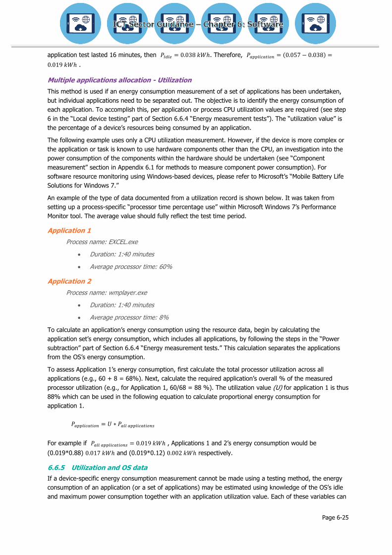
Page 6-25
application test lasted 16 minutes, then 𝑃𝐼𝑑𝑙𝑒 = 0.038 𝑘𝑊ℎ. Therefore, 𝑃𝑎𝑝𝑝𝑙𝑖𝑐𝑎𝑡𝑖𝑜𝑛 = (0.057 − 0.038) =
0.019 𝑘𝑊ℎ .
Multiple applications allocation - Utilization
This method is used if an energy consumption measurement of a set of applications has been undertaken,
but individual applications need to be separated out. The objective is to identify the energy consumption of
each application. To accomplish this, per application or process CPU utilization values are required (see step
6 in the “Local device testing” part of Section 6.6.4 “Energy measurement tests”). The “utilization value” is
the percentage of a device’s resources being consumed by an application.
The following example uses only a CPU utilization measurement. However, if the device is more complex or
the application or task is known to use hardware components other than the CPU, an investigation into the
power consumption of the components within the hardware should be undertaken (see “Component
measurement” section in Appendix 6.1 for methods to measure component power consumption). For
software resource monitoring using Windows-based devices, please refer to Microsoft’s “Mobile Battery Life
Solutions for Windows 7.”
An example of the type of data documented from a utilization record is shown below. It was taken from
setting up a process-specific “processor time percentage use” within Microsoft Windows 7’s Performance
Monitor tool. The average value should fully reflect the test time period.
Application 1
Process name: EXCEL.exe
Duration: 1:40 minutes
Average processor time: 60%
Application 2
Process name: wmplayer.exe
Duration: 1:40 minutes
Average processor time: 8%
To calculate an application’s energy consumption using the resource data, begin by calculating the
application set’s energy consumption, which includes all applications, by following the steps in the “Power
subtraction” part of Section 6.6.4 “Energy measurement tests.” This calculation separates the applications
from the OS’s energy consumption.
To assess Application 1’s energy consumption, first calculate the total processor utilization across all
applications (e.g., 60 + 8 = 68%). Next, calculate the required application’s overall % of the measured
processor utilization (e.g., for Application 1, 60/68 = 88 %). The utilization value (U) for application 1 is thus
88% which can be used in the following equation to calculate proportional energy consumption for
application 1.
𝑃𝑎𝑝𝑝𝑙𝑖𝑐𝑎𝑡𝑖𝑜𝑛 = 𝑈 ∗ 𝑃𝑎𝑙𝑙 𝑎𝑝𝑝𝑙𝑖𝑐𝑎𝑡𝑖𝑜𝑛𝑠
For example if 𝑃𝑎𝑙𝑙 𝑎𝑝𝑝𝑙𝑖𝑐𝑎𝑡𝑖𝑜𝑛𝑠 = 0.019 𝑘𝑊ℎ , Applications 1 and 2’s energy consumption would be
(0.019*0.88) 0.017 𝑘𝑊ℎ and (0.019*0.12) 0.002 𝑘𝑊ℎ respectively.
6.6.5 Utilization and OS data
If a device-specific energy consumption measurement cannot be made using a testing method, the energy
consumption of an application (or a set of applications) may be estimated using knowledge of the OS’s idle
and maximum power consumption together with an application utilization value. Each of these variables can

Page 6-26
use either primary data or secondary data, which has more flexibility, but higher uncertainty. This section
describes methods to calculate each of these variables.
Idle and maximum power
The average idle and maximum power consumption of a device can be obtained by direct measurement or
by using secondary data (e.g., idle power of 139 watts [W] and maximum power of 238 W). Please see
Section 6.5 “OS measurement,” for methods to obtain direct or secondary data on the idle and maximum
power consumption of a device.
Utilization
In this section, utilization values are defined as the percentage of a device’s resource being consumed by an
application. This section’s definition of utilization should not be confused with that given in the “Multiple
Applications Allocation – Utilization” part of Section 6.6.4 “Energy measurement tests,” which calculates
utilization differently. Utilization values can be obtained by direct measurement. Alternatively, some software
developers publish average utilization values for applications.
To measure utilization of an application or application set, carry out a “utilization only test.” Performing this
test does not require external measuring equipment but does require commonly available software
utilization measurements. Refer to steps 1, 3, 4, 5, 6, 7, 8, and 10 in the “Local device testing” part of
Section 6.6.4 “Energy measurement tests” (other steps are for direct power measurements only).
The following example uses a CPU utilization-only measurement. However, if a device is more complex or
the application or task is known to use hardware components other than the CPU, an investigation into the
power consumption of the hardware components should be undertaken (see “Component measurement”
section in Appendix 6.1). For software resource monitoring using Windows-based devices, please refer to
Microsoft’s “Mobile Battery Life Solutions for Windows 7.”
An example of the type of data documented in a utilization record is shown below. It was taken from setting
up a process-specific “processor time % use” within Microsoft Windows 7’s “Performance Monitor” tool. The
average value should fully reflect the test time period.
Example of the type of data documented from a utilization record
Application 1
Process name: EXCEL.exe
Duration: 16:40 minutes
Average processor time: 60%
Application 2
Process name: wmplayer.exe
Duration: 16:40 minutes
Average processor time: 8%
For example, to assess Application 1’s energy consumption, the utilization value would be 60%. One
could also bind multiple applications into one application set, which, for the above example, would
equate to a utilization value of 68%. This factor can be used in the following equation to calculate
proportional energy consumption:
𝑃𝑎𝑝𝑝𝑙𝑖𝑐𝑎𝑖𝑡𝑜𝑛 = 𝑈(𝑃𝑀𝑎𝑥 − 𝑃𝐼𝑑𝑙𝑒)
For example, if the OS power consumption for Idle and Maximum had been defined as 139 W and
238 W, then for the duration of the utilization test (16:40 min) 𝑃𝐼𝑑𝑙𝑒 = 0.038 𝑘𝑊ℎ , 𝑃𝑚𝑎𝑥 = 0.066 𝑘𝑊ℎ ,
for Application 1 and 2, 𝑃𝑎𝑝𝑝𝑙𝑖𝑐𝑎𝑖𝑡𝑜𝑛 = 0.017 𝑘𝑊ℎ and 0.002 𝑘𝑊ℎ respectively.

Page 6-27
6.6.6 Transaction allocation
This section describes a simplified allocation method to calculate the energy consumption of each application
process or transaction.
This method can be used if a remote device such as a server cannot be directly accessed and/or if limited
information is available. In this case, it is acceptable to report combined OS and application power
consumption; however, this should be clearly stated and justified. The method is often used for servers
because server OSs are commonly a very small portion of overall power consumption.
We use the term “transaction” to account for multiple processes that could be counted as one transaction,
thus making accounting simpler. A transaction is one or a set of application processes unique to a request
that can be defined and accounted for within the application. For example, a CRM application serving one
external user request could be defined as a transaction. This assessment will largely depend on the task and
application being assessed. It is crucial that however the transaction is defined, all processes within the
application are accounted for. If they are not included, the total application power consumption will not be
accounted for.
An application or set of applications can concurrently perform multiple processes or transactions that may
not be directly related to the task being analyzed. Minimizing the number of processes per application when
performing power measurements is desirable and decreases the uncertainty of results; however, this may
imply that processes or transactions are independent of each other and do not share resources (i.e., create
efficiency), which may not be true. Some applications are specifically designed to be most efficient when
highly loaded with processes. Therefore, if the number of processes per application cannot or should not be
reduced, the transaction-based allocation method can be applied to an application or application set’s
energy consumption measurement (obtained using methods from either Section 6.6.4 “Energy measurement
tests” or 6.6.5, “Utilization and OS data”). This method may result in uncertain results if transactions are
unequal in terms of resource use.
The following steps should be followed:
Measure the energy consumption of the application or application set using methods from either
Section 6.6.4 “Energy measurement tests” or 6.6.5, “Utilization and OS data.”
Assess the number of transactions occurring within the application or application set. If an energy
measurement test is carried out, the definition of the number of transactions falls within the time
boundary of the test (e.g., 100 transactions in 16 minutes). If a test has not been carried out,
define the transactions within a time boundary.
After the total number of transactions have been defined (e.g., 100 transactions in 16 minutes),
those that are required for analysis should be calculated as a percentage of the total. For example
80 transactions out of 100 is 80 percent of the total transactions.
To allocate energy consumption to the relevant transactions, multiply the percentage of task-
relevant transactions by the relevant application or application set’s energy consumption kWh value.
For example, if the application energy consumption is 0.017 kWh and 80 percent of transactions are
task relevant, the task relevant energy consumption is 0.017*0.80 = 0.0136 kWh.
o Specific power consumption for the relevant tasks can also be obtained. For example, if
transaction test time was 16 minutes, (0.0136*1000)/(16/60) = 51 watts.
Energy consumption per transaction can also be calculated. Divide the total energy consumption
measured for the application or application set by the number of transactions. For example, for 100
transactions in 16 minutes where the application energy consumption is 0.017 kWh, the energy
consumption per transaction is 0.017/100 = 0.00017 kWh.
o Specific power consumption per transaction can also be obtained. For example, if the
transaction test time was 16 minutes (0.00017*1000)/(16/60) = 0.6 watts.
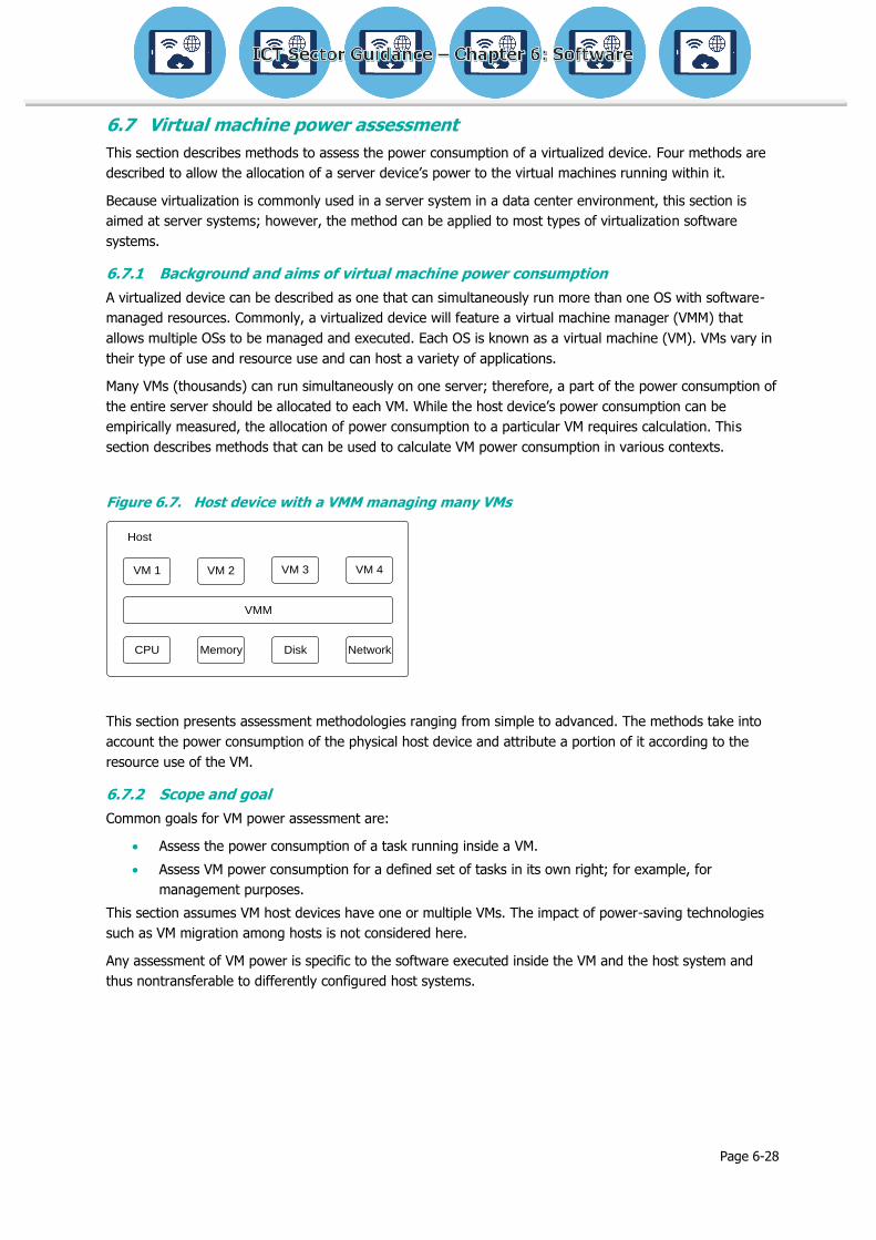
Page 6-28
6.7 Virtual machine power assessment
This section describes methods to assess the power consumption of a virtualized device. Four methods are
described to allow the allocation of a server device’s power to the virtual machines running within it.
Because virtualization is commonly used in a server system in a data center environment, this section is
aimed at server systems; however, the method can be applied to most types of virtualization software
systems.
6.7.1 Background and aims of virtual machine power consumption
A virtualized device can be described as one that can simultaneously run more than one OS with software-
managed resources. Commonly, a virtualized device will feature a virtual machine manager (VMM) that
allows multiple OSs to be managed and executed. Each OS is known as a virtual machine (VM). VMs vary in
their type of use and resource use and can host a variety of applications.
Many VMs (thousands) can run simultaneously on one server; therefore, a part of the power consumption of
the entire server should be allocated to each VM. While the host device’s power consumption can be
empirically measured, the allocation of power consumption to a particular VM requires calculation. This
section describes methods that can be used to calculate VM power consumption in various contexts.
Figure 6.7. Host device with a VMM managing many VMs
CPU Memory Disk Network
VM 1
VMM
Host
VM 2 VM 3 VM 4
This section presents assessment methodologies ranging from simple to advanced. The methods take into
account the power consumption of the physical host device and attribute a portion of it according to the
resource use of the VM.
6.7.2 Scope and goal
Common goals for VM power assessment are:
Assess the power consumption of a task running inside a VM.
Assess VM power consumption for a defined set of tasks in its own right; for example, for
management purposes.
This section assumes VM host devices have one or multiple VMs. The impact of power-saving technologies
such as VM migration among hosts is not considered here.
Any assessment of VM power is specific to the software executed inside the VM and the host system and
thus nontransferable to differently configured host systems.

Page 6-29
6.7.3 Overview of VM assessment methods
Four main methods are described to calculate the energy of a virtual machine. Because of the complexity of
virtualized devices, please refer to the process flow diagram in Figure 6.8 as a guide.
Method 1: Virtual machine manager power monitoring
The first method relies on built-in device power and resource monitoring systems to allocate VM energy
consumption.
Method 2: Virtual machine power calculation
The second method uses estimation techniques from various device power and resource statistics. This
method offers simple (Method 2a) and more advanced (Method 2b) approaches depending on data
availability. To improve the estimation method, dynamic power and resource measurements can be used
with Method 2b and are required for Method 3.
Method 3: Isolated virtual machine calculation
Method 3 focuses on direct device power and resource testing for a single VM to get high-quality, detailed
results.
Methods 2 and 3 involve a decision between dynamic and static use profiles, which is explained below.
Method 4: Transaction allocation
A further method to calculate a single transaction or process within a VM is included, which was described
as part of application measurement in Section 6.6.6 “Transaction allocation”.
Figure 6.8. Selection of a method for assessment of a virtual machine

Page 6-30
6.7.4 Method 1: Virtual machine manager power monitoring
Increasingly VMM software monitors provide live monitoring of power consumption per VM. These systems
can provide good results and replace the need to carry out in-depth assessments. However, information on
the uncertainty of their results is not widely available. Therefore, it is best to request information regarding
correct configuration and areas of uncertainty from the vendor of the virtualization solution.
6.7.5 Method 2: Virtual machine power calculation
Where VMM monitoring is not available, or is too uncertain, use Methods 2 or 3 to obtain a per-VM power
consumption.
Dynamic or static resource monitoring
When using Methods 2 or 3, decide whether the use profile is static or dynamic. The static-use profile can
be used only with Method 2a: dynamic-use profiles can be used with any other method.
Resource utilization can be measured dynamically within the virtualized device, or can be a static estimate of
average use. The total power consumption of the host device depends on the utilization of the host device
resources by each VM. Therefore, information about the levels of resource utilization by each VM is required
to allocate power consumption to a VM. Dynamic measurement is preferred because of the high variation
common in a virtualized device. The more accurate the estimate of resource use, the more certain the
result.
A static-use profile is an informed guess or average measured value of likely utilization of a device’s
resources relative to its capabilities. It represents the simplest and quickest process; data center
operators can typically provide such estimates. Hardware vendors may also be able to characterize
expected resource utilization depending on utilization of the server hardware components.
Transaction-based applications will utilize the machine depending on the number of transaction
requests. Therefore, static resource values should represent an average or typical transaction or
process set. A network service such as a dynamic host configuration protocol (DHCP) server will use
resources periodically between phases of idle time. In this case, utilization values should represent
multiple states, for example idle, average, and maximum. It should be noted that this strongly
impacts uncertainty associated with the results.
A dynamic-use profile can be either a direct monitoring of device activity or based on a
measurement of likely VM behavior, such as application load test cases or network traffic traces. A
dynamic profile is essential for performing empirical device power consumption measurements.
Method 2 – Introduction
This section describes two submethods to calculate the power consumption of a VM as a portion of total
device power based on the size of the VM relative to other VMs on the system. The device power
consumption, device utilization, and number and size of its VMs are the main inputs. Once an average VM
power consumption is calculated, the VM’s overall energy usage can be calculated by knowing the time
required for the scenario being analyzed.
The results of this method have a higher uncertainty because an estimation technique is used. When
reporting assessment results, document the applied assessment methods and note the level of uncertainty
of the results.
Before testing, follow the steps below, which describe how to prepare a virtualized device.
Virtualized device preparation
Use the following steps to prepare a virtualized device for direct assessment. Not all steps are relevant for all
methods.

Page 6-31
Define and implement a virtualized device test profile for each device. See below for steps to
complete this.
Where possible, implement a new install of the VMM and each VM.
Activate and connect relevant VMM and VM hardware services (e.g., connect to the network to
access the internet).
Where relevant, run the virtualized device and ensure that any VMM-to-VM and internal VM
exchanges and initial, one-time-only setups are completed (unless this is what is to be analyzed).
If details for each VM are required, record an OS task and service listing before and after each test
period.
A VMM resource and service listing is also required for some methods, as explained later by
method.
Setting virtualized device test and use profiles
When testing a virtualized device, define and document a device-wide test profile. This profile should
document the details of the virtualized system, such as what VMM is running and what VM’s constitute a
typical scenario for the assessment. The power consumption of each VM will vary with the utilization of the
host device’s resources by processes and applications. Thus during the assessment, each VM should be
running a typical operational profile of the OS and applications. This use profile determines the resource
utilization of the host system. The processes and their resource utilization over time are referred to as the
“application task profile.” For example, the profile could show the system is running an online web shop
system with a specified number of concurrent users.
A test profile can either represent a real workload or a synthetic workload composed of smaller units of
work. Ideally, the typical application profile of a VM will match historical use. An assessment of VM power
consumption based on a representative test profile will reduce uncertainty associated with the results. In
some cases instead of developing a custom test profile it is recommended using an existing profile that
closely matches the anticipated VM application. For web applications, popular test profiles are provided by
organizations such as the Transaction Processing Performance Council,1 the Standard Performance
Evaluation Corporation (SPEC),2 and the Storage Performance Council.3
Method 2a: Single data point power consumption (secondary data)
This method involves calculating the average device power consumption and the size of the VM being
analyzed.
Average power consumption calculation
If no primary measurement data is available, the average server power consumption calculation should rely
on secondary data. Any reported power consumption depends on the precise server configuration of
hardware as well as software. Data, which is often reported in different ways, should be standardized to the
average power consumption using the following method.
When sourcing secondary data, it should be based on a close match to the device’s hardware. Important
hardware configuration aspects that impact power consumption are: the number and type of CPUs, the
amount and type of installed memory, the number and make of hard disks and network controllers, the
mainboard model, and the model and number of power supply units. Important software configuration
1 Transaction Processing Performance Council, http://www.tpc.org/
2 Standard Performance Evaluation Corporation, http://www.spec.org/
3 Storage Performance Council, http://www.storageperformance.org/home/

Page 6-32
options impacting power consumption are the basic input/output system (BIOS) configuration and the VM
host configuration. The uncertainty associated with host power values depends on the similarity of the host
system to those configuration options.
Average power consumption can be estimated from single points, although this results in increasing
uncertainty. Manufacturers publish the maximum measured electricity (MME) value, which is the maximum
observed power consumption by a server model. The MME can often be calculated with online tools, which
may allow the specification of individual components for a particular server configuration. Based on these
estimations of maximum power consumption, the average power consumption is commonly assumed to be
60 percent of MME for high-end servers and 40 percent for volume and mid-range servers.
Figure 6.9. Correlation between server host resource utilization and power consumption
If the MME cannot be found, three other measures of power consumption published by server
manufacturers are commonly used: power supply maximum rated input power (MRIP), power supply output
power (OP), and server typical power (TP). The most accurate is MME because it is directly related to the
server’s individual hardware setup. If the MME listing is not available, methods for calculating it from the
three alternative power listings are shown in Table 6.1.
Table 6.1. Three ways to calculate the MME from power consumption values listed by
manufacturers
Power
consumption type
Power supply
maximum rated
input power
(MRIP)
Power supply
output power
(OP)
Server typical
power (TP)
Server maximum
measured electricity
(MME) calculation
MME = (MRIP * PUV)
/ SUV
MME = ((OP/PSE)*
PUV) / SUV MME = TP / SUV
SUV = system utilization value (0.40 & 0.66 for volume and mid-range and high-end servers
respectively)
PUV = power supply utilization value (0.25, 0.30, and 0.40 for volume, mid-range, and high-end
servers respectively)
PSE = power supply efficiency value (0.75 for 50 percent load, 0.85 – 0.92 for 50 percent load)
(Williams and Tang, 2011. See footnote 7).
0102030405060708090
100
0 10 20 30 40 50 60 70 80 90 100
Po
we
r (W
)
Utilization (%)
Old Model
New Model

Page 6-33
Calculating VM size
The “size” of the VM is its share of the server’s total computational power. For this method, VM size is
reported as a percentage: for example, a server has three VM’s, two using 25 percent and one using 50
percent of its computational power. The size of a VM can change; for example, if a VM that provided a
service for eight hours a day is now used for only a few hours a day, it would become “smaller.” In such a
case, the average aggregate size over a sufficiently long time period should be estimated.
Note that a VM uses a higher proportion of computational capacity on a server with a smaller capacity than
on one with a larger capacity. Finally, the sum of the size of all VMs on a server is equal to 1 since the total
typical power consumption of the server should be accounted for.
𝑃𝑉𝑀 = 𝑠𝑖𝑧𝑒𝑉𝑀 ⋅ �̂�, i.e., power of the VM is proportional to the size of the VM and the average server
power consumption.
VM size can be either directly assessed or estimated. If the device is located within a data center
environment, the VM size should be known to the data center operatives. Most VMMs provide real-time
monitoring of resource utilization per VM. These monitoring systems offer the most accurate data on the
resources VMs use during operation.
Method 2b: Dynamic power consumption calculations
This method involves more than one power consumption data point for the device being analyzed and is
suited to primary data collection although secondary data can be used. Key data required for this method is
the device utilization, the size and number of VMs, and the device’s dynamic power range.
Device utilization
Device utilization depends directly on the type of service provided by the server and the service demand. It
can often be estimated by the data center operator. Notably, uncertainty of the server utilization results in
uncertainty of the average power consumption. A precise correlation of utilization of components to overall
system power is specific to the server configuration in hardware and software. For the purpose of this
assessment, and accepting significant levels of uncertainty, CPU load can be used as a proxy for overall
device utilization. If possible in a specific context, the weighted influence of other components can be
included in the utilization value, provided the assumptions leading to the adoption of such weightings are
documented.
Depending on the workload of the server device, utilization varies between 40 and 60 percent of the
maximum power consumption (see Figure 6.9). This variation depends on the utilization of the most energy-
consuming components, notably, CPU, memory bus and disk, and network I/O. Using primary utilization
data from components will improve the precision of the results.
Dynamic power consumption
Calculating the dynamic power consumption range requires knowing the device’s idle and peak power
consumption values. Idle, or base, power consumption is when the VMM is operating but no VMs are
executed on the system. Peak, or maximum, power consumption is the maximum possible when all
components are fully utilized. Figure 6.9 illustrates the levels of base power 𝑃𝑏𝑎𝑠𝑒 and peak power 𝑃𝑝𝑒𝑎𝑘
consumption. The difference between these values is the dynamic power range 𝑃𝑑𝑦𝑛. Given the relatively
high uncertainty associated with any estimation method, it can be assumed that the servers’ power
consumption increases linearly with increasing CPU load, which, however, introduces additional uncertainty.
The preferred data can be obtained using the methods described in Appendix 6.1 – “Measurement methods”
(see the examples below for types of data required). Secondary data should be used only if an assessment
of power consumption over a range of utilization values can be found for a specific model. Possible sources
are Energy Star and SPEC power test results. Single data point estimates should not be used to estimate the
idle or maximum power consumption.

Page 6-34
Power Consumption per VM
Once the dynamic range has been determined, the device (server) utilization can be applied to the
calculation of average power consumption. Device utilization (as a percentage) can be correlated to a power
consumption value in the interval between idle and maximum power consumption.
When calculating the dynamic power consumption relative to base power consumption, the latter should be
allocated explicitly to all VMs on the server. A simple procedure is to uniformly allocate to all 𝑛 VMs.
The size and number of VMs can be calculated using Method 2a of this section.
With the device utilization, the size and number of VMs, and the device’s dynamic power range collected,
the VM power consumption can be calculated. For the power consumption of the VM being analyzed, use
the following equation:
𝑃𝑉𝑀𝑥 = 𝑈𝑉𝑀𝑋⋅ 𝑠𝑖𝑧𝑒𝑉𝑀𝑋
⋅ 𝑃𝑑𝑦𝑛 +𝑃𝑏𝑎𝑠𝑒
𝑛
where 𝑃𝑉𝑀𝑥 is the power consumption of the VM being analyzed, 𝑃𝑑𝑦𝑛is the dynamic power range of the
device, 𝑈𝑉𝑀𝑥 is the utilization of the VM, 𝑠𝑖𝑧𝑒𝑉𝑀𝑥 is the size of the VM being analyzed, and 𝑛 is the number
of VMs running on the server.
The following examples illustrate the above method.

Page 6-35
Example 1: Utilization of a webserver
Table 6.2. Example 1 - Utilization of a webserver
Parameter Value
Model IBM x
Power by IBM
configurator
Idle 860 W, Max load 1500 W
Type of application Web server for web shop
Peak demand 10 requests/second
Number of VMs 3
Figure 6.10. Average utilization of a webserver over 24 hours
From a web shop’s experience with its old server, it is assumed that its new IBM server used in
production will have a peak utilization of roughly 50% of server power and off-peak utilization of
10%. Each VM is approximately the same size, that is, 33%. Peak utilization was measured to occur
for an average of 9 hours per day.
Thus the power consumption during peak utilization is roughly 640 ⋅ 0.33 ⋅ 0.5 +860
3= 390𝑊.
0
10
20
30
40
50
60
0 2 4 6 8 10 12 14 16 18 20 22
Uti
lizai
ton
(%
)
Time (Hours)

Page 6-36
Example 2 – Internal enterprise resource planning (ERP) system server
The data below was obtained from the owner of a company’s internal server system. The system runs
at this level 8 hours per day.
Table 6.3. Example 2 — Internal ERP system server
Parameter Value
Server Type Fujitsu xx
Base power from web site 600W
Max power from web site 1200W
VMs VM1 – DNS
VM2 – DHCP
VM3 – ERP
Average utilization of ERP server at
peak (7 a.m. - 6 p.m.)
30%
Average utilization of ERP server at
off-peak
10%
VM size estimation:
The size estimation was performed by the data center manager from his personal
experience. He estimated the size as:
DHCP (dynamic host configuration
protocol)
5% constant
DNS (domain name system) 5% constant, additional 3% during office
hours
ERP (enterprise resource planning) Dominates utilization – allocate all
resources except DHCP and DNS =>
87%
Thus the peak power consumption for the ERP VM can be calculated as: 𝑃𝑉𝑀1 = 356 𝑊
At off-peak, the power consumption is roughly 250 W, which results in an average daily power
consumption of 300 W.

Page 6-37
Dynamic power and resource measurements
To improve the estimation method, dynamic power and resource measurements can be used with Method
2b and are required for Method 3.
Device power measurement
If a dynamic-use profile is used, the device’s power consumption should be dynamically measured for the
period of the test. External measurement of server system power (see Appendix 6.1 – “Measurement
methods”) can be performed with power-monitoring power-distribution units or power-supply units on the
server. Alternatively, an increasing number of server systems provide power-monitoring capability via Simple
Network Management Protocol (SNMP)4 or Advanced Configuration & Power Interface (ACPI).5
If measurements cannot be taken, average power consumption values can be estimated from sources such
as Energy Star or the manufacturer’s online tools. Using these values will decrease result certainty. Any
reported power consumption depends on the precise server configuration of hardware as well as software.
Therefore, when sourcing data, use data that closely match the device’s hardware. Online manufacturer
tools are preferable to standard secondary data sources: they allow one to specify individual components
and create a virtual copy of the machine being analyzed.
Dynamic VM resource utilization measurement
A dynamic VM resource utilization measurement provides a more accurate assessment of per-VM power
consumption. Such an assessment allocates power consumption of the host device to individual VMs based
on their share of utilization of the hardware components. This assessment requires measuring each VM’s
level of utilization of device components over time and relating that to the total power consumption of the
device. This data can then be used with the equations in Methods 2a and 2b to gain more precise results.
A benefit of using dynamic rather than static values is that they measure the variation of power
consumption over time. For example, a VM could be analyzed per second or a set of VMs could be assessed
every minute for eight hours per component. For server systems, the most important components regarding
power consumption are the CPU, the memory and communication bus on the mainboard, the hard disk, and
the network interfaces.
Most VMMs provide real-time monitoring of resource utilization per VM.6 These monitoring systems give the
most accurate data on the resources that VMs use during operation.
If utilization measurements cannot be undertaken, but power consumption measurements can, then
“Method 3: Isolated virtual machine calculation,” can be used. This method is closely related to those
applicable to consumer measuring tools described in Appendix 6.1 – “Measurement methods.” Also see
Section 6.5 “OS measurement,” in particular the “Idle tests” and “Maximum power tests” subsections of
6.5.4 “Energy measurement tests,” which contain further guidance.
4 Simple Network Management Protocol, http://www.ietf.org/rfc/rfc1157.txt.
5 Advanced Configuration & Power Interface, http://www.acpi.info/.
6 E.g., VMWare web services, Oracle Server Console, Microsoft Hyper-V Console, etc.

Page 6-38
6.7.6 Method 3: Isolated virtual machine calculation
Method 3 describes how a defined test profile can be used to directly assess the power consumption of a
VM. For this method, a service application is executed inside an isolated VM. It yields accurate results;
however, it may incur time and device delays because of the need to perform specific tests.
This method calculates the power consumption of a VM where only one VM is being run. It should be used if
a single VM out of many is required to be analyzed in detail. It requires a dynamic-use profile and involves
directly measuring the host device power. Running the VM in isolation to other VMs allows allocation of all
power consumption to that VM. The device’s idle power consumption can be measured when no other VM is
being executed. This idle power is then allocated to the VM in proportion to the number of VMs running on
the server.
The following steps should be followed:
Measure the host device’s idle or base power when only the VMM is running, that is, the target VM
and all other VMs on the host are suspended.
Run the VM with the defined application use profile and measure host power over a time interval
that is representative of the average host performance.
Calculate the average power measured during the testing process.
Calculate 𝑃𝑉𝑀𝑥 = (�̂� − 𝑃𝑖𝑑𝑙𝑒) +𝑃𝐼𝑑𝑙𝑒
𝑛, where 𝑃𝑉𝑀𝑥 is the power consumption of the VM being
analyzed, �̂� is the average power consumption during the measurement period when only the VM is
running, 𝑃𝑖𝑑𝑙𝑒 is the power consumption of the device in an idle state, and 𝑛 is the number of VMs
of the device in deployment.
The following example illustrates the calculation.
Example 3 Isolated VM calculation
Table 6.4. Example 3 – Isolated VM calculation
Parameter Value
Idle power (with only VMM running) 205 W
Average device power over the time period
specified in the application use profile
when the measurement test is carried out
380 W
Average number of VMs running during
average use per device
6
𝑃𝑉𝑀𝑥 = (380 − 205) +205
6

Page 6-39
6.8 Case studies
6.8.1 Electronic software distribution
A methodology and case study regarding the impacts of moving from a physical to digital distribution chain
by Williams and Tang (2011)7 uses the methodologies in this chapter to calculate the impacts of the digital
supply chain.
6.8.2 Office productivity cloud services
Williams and Tang (2013)8 performed a rigorous and detailed energy consumption analysis of three cloud-
based office productivity applications. They analyzed the power consumption of the data center, network,
and user devices that access the cloud service. The study also performed an energy consumption analysis
on “traditional” noncloud versions of the software to understand the overall impact of cloud services.
6.8.3 Quantifying the GHG impact of Microsoft Windows OS
A methodology to calculate the energy consumption of one PC or an enterprise of PCs has been developed
into a useable modeling tool. Energy consumption is modeled according to variables that profile the user
base, devices, and power management set-up. Thus the modeling tool can assess the impacts of potential
changes in hardware, power management, and OS type.
The modeling tool is based on a Microsoft Windows environment and thus may not be suitable for all device
types. The model was designed by Dan Williams in conjunction with Microsoft UK and the University of
Reading.9
6.8.4 Designing power-efficient software
Many software developers publish guidelines on how to design more energy-efficient software. Microsoft’s
“Energy Smart Software” is a good guide to them.10 Microsoft has a wealth of resources for designing
energy efficient software on its developer websites.
6.8.5 Microsoft Internet Explorer 9 measurement
Microsoft performed power monitoring of its Internet Explorer 9 software using methods similar to those in
this chapter. It provides a useful case study.11
7 D.R. Williams, and Y.Tang, “Methodology to Model the Energy and Greenhouse Gas Emissions of Electronic Software
Distributions,” Environmental Science & Technology 46, no 2, November 2011:1087–1095, available at: http://pubs.acs.org/doi/abs/10.1021/es202125j 8 D. R.Williams and Y. Tang, “Impact of Office Productivity Cloud Computing on Energy Consumption and Greenhouse Gas
Emissions,” Environmental Science & Technology 47, no. 9, April 2013:4333–4340, available at: http://pubs.acs.org/doi/abs/10.1021/es3041362
9 The model can be found at: http://www.microsoft.com/uk/environment/calculators.aspx
10 Microsoft, Energy Smart Software, Microsoft Corporation, June 2010, available at: http://msdn.microsoft.com/en-
us/windows/gg463226 11 http://blogs.msdn.com/b/ie/archive/2011/03/28/browser-power-consumption-leading-the-industry-with-internet-explorer-
9.aspx

Page 6-40
Appendix 6.1 - Measurement methods
This appendix describes how to measure a device’s power consumption. Two direct and two indirect
methods are described. The first direct method, “total device measurement,” is simpler, but provides little
detail into what part of the system consumes how much power and gives results with greater uncertainty.
The second direct method, “power measurement per device component,” is more complex, but provides
insights into which components are using more power and thus allows efficiency to be tailored.
If the scenario being analyzed does not permit access to the device, secondary power consumption sources
can be used. Secondary data should be used only if it was measured using a comparable OS and application
set. Secondary data methods are described in each of the OS and application methodology sections. For
servers, a common method to estimate power consumption uses online manufacturer calculators—see
Section 6.7 for more details.
Software power consumption can also be measured without access to the device. Software power
consumption is commonly estimated. However, some hardware devices have easy-to-use, built-in power
consumption measurement systems.
The first step in measuring the power consumption of software involves defining the device used in the
measurement. The device will ultimately determine the range of power consumption because its hardware
components run at specified power levels.
Figure A6.1.1 Decision tree for selecting an appropriate measurement tool
Direct measurement tools
Direct measurement of power consumption requires a device, such as a wattmeter, multimeter, or
oscilloscope, which samples the voltage and current and reports the power consumption (watts) and energy
consumption (watt hours). Care should be taken to control the environment in which the test is performed.
Ambient room temperature and humidity levels should be within the normal range for the hardware in the
test scenario. These variables, along with mains voltage supply and test equipment models used, should be
accurately recorded in case a retest is needed. It is strongly recommended that before measurement the
following IEC guidelines are understood and followed:

Page 6-41
IEC 62301 ed2.0 - Measurement of standby power.12
IEC 62087-BD ed3.0 - Methods of measurement for the power consumption of audio, video and
related equipment.13
The device used for power measurement should be capable of performing and recording measurements
over a defined time period. For exact meter specifications, refer to the IEC documents.
Total device measurement—mains-powered devices
This method should be used if the device being analyzed is powered by mains (AC) electricity only. It should
not be used if the device can be powered from an integrated battery that could skew measurements when
charging. If the device contains a battery, remove it and, if possible, power from a mains (AC) power
adapter instead. Place the power measurement device (as defined in Section “Direct measurement tools”
above) between the mains (AC) outlet and the power adapter. This placement will ensure that the losses
encountered by power supply units do not skew the result. The energy measurement test processes in Part
B can then be carried out and the results recorded.
If a device has multiple processing systems (such as a rack server), see Section 6.7 “Virtual Machine power
assessment.”
Total device measurement—battery-powered devices
If the device is powered directly from an on board battery, measurement is by one of two methods. The first
involves a battery run-down test, which, while simple, can be time consuming and gives high uncertainty
levels because of its reliance on specific hardware parameters and software measures. The second involves
the bespoke creation of a battery extension. This requires technical skills, but provides reliable power
consumption information.
Battery run-down
The battery run-down test involves measuring how much time the device’s battery takes to fully discharge
from a state of full charge. This test will provide only the average power consumption value. To carry out
this test, the following information is required:
𝐶 = Listed battery capacity (milliamp hour [mAh] or Wh)
𝑉= Battery voltage
𝑡 = Time taken to discharge (hours)
Conversion = 𝐶𝑊ℎ = 𝑉 ∗𝐶𝑚𝐴ℎ
1000
𝜂 (eta) = the efficiency of the charge cycle (%).
This information can then be used with the following equation to assess the average power consumption:
𝑃𝑠𝑦𝑠𝑡𝑒𝑚 =(
𝐶𝑊ℎ
𝑡)
𝜂
Where 𝑃𝑠𝑦𝑠𝑡𝑒𝑚 is the average power consumption of the system in watts.
Example:
𝐶 = 4400 𝑚𝑖𝑙𝑙𝑖𝑎𝑚𝑝 ℎ𝑜𝑢𝑟𝑠 [𝑚𝐴ℎ]
𝑉 = 11.1 𝑉
12 Available from: http://webstore.iec.ch/webstore/webstore.nsf/Artnum_PK/44782 13 Available from: http://webstore.iec.ch/Webstore/webstore.nsf/Artnum_PK/45001

Page 6-42
𝑡 = 2.5 ℎ𝑜𝑢𝑟𝑠
Conversion = 𝐶𝑊ℎ = 49 𝑊ℎ
𝜂 (eta) [efficiency] = 70%
𝑃𝑠𝑦𝑠𝑡𝑒𝑚 = 27.91 𝑊
The results can be affected by many factors, the main one being the battery capacity, which can decline
with age. A new battery should be used for these tests. If possible, battery capacity should be measured
using appropriate tools (software or hardware) instead of using the listed value.
Charging efficiency can also skew results. As the battery charges, the charging hardware (converter, charge
circuitry, and battery) lose some power mainly to heat discharge. Charging efficiency is, therefore, the
difference in the amount of power that is consumed by the device and the power used to charge the
battery. For example, an efficiency of 70 percent means that 30 percent of the total power used to charge a
battery is lost as heat. Average efficiency values of 60 percent14 for laptop devices and 30 percent15 for
mobile devices can be used.
The test scenario should be run for the entire time required to discharge the battery. For a device with a
long discharge time or where the task is time dependent, this may become impractical. To overcome this
limitation, software that can estimate the capacity of a battery can be used. This software can read capacity
at the start and end of a task. The difference can be substituted for C in the above formula along with the
time taken to perform the task. This method offers results with higher levels of uncertainty because the
capacity of the battery is only estimated via software.
Battery extension
The battery extension method involves the bespoke, nonpermanent, extension of a device’s internal battery
via an external battery holder and wiring array. This extension allows placement of a power measuring
instrument between the hardware device and the device’s battery. Because this method requires technical
hardware skills, it should only be performed by an approved electrical technician on hardware that has been
approved for test purposes.
The technical details of this method are device specific; however, the following basic steps can be followed:
Create a replacement battery shell that contains relevant electrical contacts and a wiring loom to
which the measurement device can attach.
Create a new battery holder that contains relevant electrical contacts in which the original battery
can safely sit.
Ensure that the extension does not interfere with the normal operation of the device or the battery.
Note that the use of some measurement devices may increase the overall power consumption of
the battery, but this may account for less than 1 percent of total.
When testing mobile phones or low-powered devices, use high-quality power measurement probes
(<1 millisecond [ms] per measurement) to assess the high-frequency components.
14 Suzanne Foster, Chris Calwell, Travis Reeder, et al., “Battery Chargers and Energy Efficiency: Summary of Findings
and Recommendations,” Natural Resources Defense Council (NRDC), August 2003, available at:
http://www.efficientproducts.org/reports/bchargers/NRDC_Battery_Charger_Final.pdf
15 J. Ruutu, J.K. Nurminen, and K. Rissanen, ”Energy Efficiency of Recharging a Mobile Device,” Proceedings of the Fifth
International Conference on Next Generation Mobile Applications, Services and Technologies, Next Generation Mobile Applications, Services and Technologies (NGMAST), Cardiff, September 2011, pp. 175–79.

Page 6-43
For a case study, please see Rice and Hay (2010).16
Component measurement
Component measurement offers greater insights into the power consumption of different hardware
components when running software. Software, depending on its type and design, uses different hardware
components or requires different amounts of energy from basic components: for example, a graphics
software package uses the graphics processing unit (GPU) of a device more intensively, increasing its overall
power consumption. This analysis can lead to targeted hardware tuning or investments to reduce power
consumption.
In component measurement, a power measurement tool is attached to each component of the analyzed
device to measure its power consumption while the software is running. Some devices contain onboard
component measuring, which act as a built-in power measurement tool, simplifying the process.
Component measurement apparatuses are common in large ICT developer organizations. If an official
component measurement apparatus is not available, the subsequent basic steps should be followed to
measure hardware components. Because the hardware will be disassembled, a registered technician should
carry out the procedures. The hardware does not have to be modified, although this depends on hardware
design and the level of component detail needed.
The method can be used with devices powered via mains (AC) or battery electricity. However, it requires
technical hardware skills and should be performed only by an approved electrical technician on hardware
that has been approved for test purposes.
To conduct the test, identify the device components using a device data sheet. Some components, such as a
hard drive and cooling fan, have exposed wires on which measurement devices can be used. If the
component cannot be measured but can be removed, a method of subtractive allocation can be used. If the
component is soldered or plugged into the device’s electrical boards, such as processor or memory, a
decision should be made to either extend the component so that measurement can be made possible, or
amalgamate the components’ power consumption. See Mahesri and Vardhan, “Power Consumption
Breakdown on a Modern Laptop,”17 for methods to allocate CPU, memory, and graphics when amalgamating
readings. For miniaturized devices, such as smart phones, this method may not be suitable and specialized
measurement equipment may be needed.
Classify the components into the following categories:
Directly measureable: Components that can be measured with a power-measurement device.
Indirectly measureable – nonremovable: Components that cannot be measured and are
essential to the running of the software system.
Indirectly measureable – removable: Components that cannot be measured but can be
removed without stopping the running of the software system.
Measure overall system power using a power-measurement device at the exit of the power supply unit to
account for efficiency losses. Use a power measurement device to calculate the power consumption of each
component or grouping of components. Identify the power supply wires using component data sheets.
If the subtractive allocation method is used to measure removable components, measure the system power
before and after the hardware is connected and allocate the difference to the component being analyzed.
16 A. Rice and S.Hay, “Measuring Mobile Phone Energy Consumption for 802.11 Wireless Networking,” Pervasive and Mobile
Computing 6, Issue 6, December 2010: 593–606, available at: http://www.cl.cam.ac.uk/~acr31/pubs/rice-80211power.pdf 17 A. Mahesri, and V. Vardhan, “Power Consumption Breakdown on a Modern Laptop,” Proceedings of the 4th International
Conference on Power-Aware Computer Systems, PACS 2004, Portland, December 2005, pp. 165–80.

Page 6-44
The final step is to account for the energy efficiency between the mains (AC) supply and the power supply
to the component. This may be achieved by applying a known efficiency value from manufacturer
specifications. If this specification is not known, it may be measured by placing an extra power supply
measurement device on the mains (AC) supply output and comparing the measurement to that of the
component device that supplies power to each individual component (e.g., the power supply unit in a PC).
The amount of power used by each component should be divided by the efficiency value (i.e., 34 W /80%)
to provide a true power consumption value.

Whilst reasonable steps have been taken to ensure that the information contained within this publication is correct, the authors, the Carbon Trust, its agents, contractors and sub-contractors give no warranty and make no representation as to its accuracy and accept no liability for any errors or omissions. Any trademarks, service marks or logos used in this publication, and copyright in it, are the property of the Carbon Trust. Nothing in this publication shall be construed as granting any licence or right to use or reproduce any of the trademarks, service marks, logos, copyright or any proprietary information in any way without the Carbon Trust’s prior written permission. The Carbon Trust enforces infringements of its intellectual property rights to the full extent permitted by law. The Carbon Trust is a company limited by guarantee and registered in England and Wales under company number 4190230 with its registered office at 4th Floor, Dorset House, Stamford Street, London SE1 9NT. Published in the UK: 2017 © The Carbon Trust 2017. All rights reserved.
ICT Sector Guidance