Chapter 1 Huﬀman Coding - Steven Pigeonstevenpigeon.com/Publications/publications/Huffman... ·...

Chapter 1

Huffman Coding

Steven Pigeon

Universite de [email protected]

1.1 Introduction

Codes may be characterized by how general they are with respect to thedistribution of symbols they are meant to code. Universal coding techniquesassume only a nonincreasing distribution. Golomb coding assumes a geo-metric distribution [1]. Fiala and Greene’s (start, step, stop) codes assumea piecewise uniform distribution function with each part distributed expo-nentially [2]. Huffman codes are more general because they assume nothingparticular of the distribution; only that all probabilities are non-zero. Thisgenerality makes them suitable not only for certain classes of distributions,but for all distributions, including those where there is no obvious relationbetween the symbol number and its probability, as is the case with text. Intext, letters go from ’a’ to ’z’ and are usually mapped onto a contiguousrange, such as, for example, from 0 to 25 or from 97 to 122, as in ASCII, butthere is no direct relation between the symbol’s number and its frequencyrank.

There are various ways of dealing with this situation. One could be that

1

CHAPTER 1. HUFFMAN CODING 2

we build a permutation function that maps the arbitrary symbol numbersto their ranks, giving us an effectively nonincreasing distribution. Once thisdistribution is obtained, we could use one of the aforementionned codes todo the actual coding. Since it is unlikely that the distribution obtainedmatches exactly one of the distributions assumed by the simpler codes, acertain inefficiency is introduced, in addition to the storage of the permu-tation information. This inefficiency may lead to an unacceptable loss ofcompression. Huffman was the first to give an exact, optimal algorithm tocode symbols from an arbitrary distribution [3]. In this chapter, we will seehow this algorithm manages to produce not only efficient but optimal codes.We will also see some adaptive algorithms that will change the codebook assymbol statistics are updated, adjusting themselves as probabilities changelocally in the data.

1.2 Huffman Codes

Huffman codes solve the problem of finding an optimal codebook for an arbi-trary probability distribution of symbols. Throughout this chapter, we willuse the following conventions. The uncompressed string of symbols will bethe message and its alphabet will be the original or message alphabet. Thecompressed output will be composed of output symbols. We will call a code

a string of output symbols associated with a message symbol, and a code-

book will be the set of all codes associated with all symbols in the messagealphabet. A codebook can be seen as a function F mapping symbols in A,the message alphabet, to a subset of B+, the set of all (non-empty) stringscomposed from the output alphabet B, in a nonambiguous way.

There are, of course, many different ways of devising codebooks. How-ever, Huffman’s algorithm produces optimal codebooks, in the sense thatwhile there might exist many equivalent codebooks, none will have a smalleraverage code length. Note that this is true when we respect the implicitassumption that each code is composed of an integer number of output sym-bol, and that each symbol receives a distinct code, which may not be truefor all types of codes. Think of arithmetic coding, where the algorithm isable to assign a fractional number of output symbols to a code. There-fore, in the context of Huffman coding, “variable-length codes” really meansvariable-integer -length codes. In this section, we will be concerned with the


construction of Huffman codes and their efficiency. We will also see thatwhile we generaly intend the output alphabet to be B = 0, 1, the onlyrequirement is that the output alphabet contains at least two symbols.

1.2.1 Shannon-Fano Coding

Shannon and Fano [4] separately introduced essentially the same algorithmto compute an efficient codebook given an arbitrary distribution. This al-gorithm is seductively simple. It goes as follows: First sort all the symbolsin nonincreasing frequency order. Then split this list in a way that the firstpart’s sum of frequencies is as equal as possible to the second part’s sumof frequencies. This should give you two lists where the probability of anysymbol being a member of either list is as close as possible to one half. Whenthe split is done, prefix all the codes of the symbols in the first list with 0 andall the codes of the symbols of the second list with 1. Repeat recursively thisprocedure on both sublists until you get lists that contain a single symbol.At the end of this procedure, you will get a uniquely decodable codebookfor the arbitrary distribution you input. It will give a codebook such as thatshown in Table 1.1 a).

There are problems with this algorithm. One of these is that it is notalways possible to be sure, because we proceed greedily, how to split thelist: cuting in a way that minimizes the difference of probability betweenthe two sublists do not always give the optimal code! An example of aflawed codebook is given in table 1.1 b). While this algorithm is conceptuallyattractive because it is simple, it sometimes gives codebooks that are muchworse than those given by Huffman’s algorithm for the same distribution.

1.2.2 Building Huffman Codes

Huffman in his landmark 1952 paper [3] gives the procedure to build optimalvariable length codes given an arbitrary frequency distribution for a finitealphabet. The procedure is built upon a few conditions that, if satisfied,makes the codebook optimal. The first conditions are as follows:

(a) No code is a prefix of another code.

(b) No auxiliary information is needed as delimiter between codes.


Symbol Frequency Code Symbol Frequency Codea 38416 00 a 34225 000b 32761 01 b 28224 001c 26896 100 c 27889 01d 14400 101 d 16900 100e 11881 1100 e 14161 101f 6724 1101 f 4624 110g 4225 1110 g 2025 1110h 2705 1111 h 324 1111

a) b)

Table 1.1: Examples of Shannon-Fano codes for 8 symbols. a) a codebookwith codes of average length 2.67. The entropy of this distribution is 2.59bits/symbol. Discrepancy is only 0.08 bits/symbol. b) an example of aShannon-Fano codebook for 8 symbols exhibiting the problem resulting fromgreedy cutting. The average code length is 2.8, while the entropy of thisdistribution is 2.5 bits/symbol. Here, discrepancy is 0.3 bits/symbol. Thisis much worse than the discrepancy of the codes shown in a).

The first requirement implies that, for a series of bits, there is a uniqueway of decoding it. This leaves no ambiguity as to the encoded message. Thesecond requirement tells us that we do not need markers, or special symbols(such as the “space” symbol in the seemingly binary Morse code),1 to markthe begining nor the end of a code.

One way to satisfy both requirements is to build a tree-structured code-

book. If the codebook is tree structured, then there exist a full binary tree (abinary tree is full when each node either is a leaf or has exactly two children)with all the symbols in the leaves. The path from the root to a leaf is thecode for that leaf. The code is obtained by walking down the path from theroot to the leaf and appending to the code a 0 when we go down left or a 1when we go down right. Reaching a leaf naturally delimits the code, thus sat-isfying the second requirement. Were we allowed to address internal nodes,

1In Morse code, one uses strings of dots (·) and dashes (–) to encode letters, but thecodes are separated by spaces. The duration of a dot or a space is a third of that of adash.


there would be codes that are prefixes of other codes, violating requirementa). The first requirement is therefore met because no codes are assigned tointernal nodes; codes designate only leaves.

Let A = a1, a2, . . . , an be our alphabet for which we want a code. Werearrange the alphabet A so that symbols are listed in order of nonincreasingfrequency. This convention prevents us from using a permutation functionπ(i) that gives the index in A of the symbol that occupies rank i. This wouldneedlessly complicate the notation. This rearranged alphabet satisfies

P (a1) > P (a2) > · · · > P (an) (1.1)

where P (a) is a shorthand for P (X = a), and X is our random sourceemitting the symbols. For this alphabet, we want to build a optimal set ofcodes with lengths

L(a1) 6 L(a2) 6 · · · 6 L(an) (1.2)

It turns out that we will have to slightly modify eq. (1.2). Let Ln bethe length of the longest code. Let us suppose that there are more thantwo codes of length Ln that do not share prefixes of length Ln − 1 amongthemselves. Since by hypothesis we already have an optimal code, there areno other codes that are prefixes of the codes of length Ln. Since the codes oflength Ln share no prefix between them and there are no other codes that areprefixes to any of the length Ln codes, it means that these codes of length Ln

have at least one extra bit, making them too long. Therefore, Ln should beLn − 1, a contradiction! What this means is that we can drop the last bit onall these length Ln codes. This in turn implies that at least two of the longestcodes of length Lmax must share a prefix of length Lmax − 1. The same kindof argument will prevent an algorithm that builds an optimal codebook fromgiving extra, useless bits to codes. Equation (1.2) becomes

L(a1) 6 L(a2) 6 · · · 6 L(an−1) = L(an) (1.3)

where the last 6 is now =. We now have the following conditions to satisfy:

(a) No code is a prefix of another code.

(b) No auxiliary information is needed as delimiter between codes.


(c) L(a1) 6 L(a2) 6 · · · 6 L(an−1) = L(an) .

(d) Exactly 2 of the codes are of length Lmax are identical except for theirlast bit.

(e) Every possible code of lengths Lmax − 1 is either already used or haveone of its prefixes used as a code.

Surprisingly enough, these requirements will allow a simple algorithm tofulfill them. The key requirement is requirement c). While Huffman codesgeneralize to any number of coding digits greater than 1, as we will see inSection 1.2.3, let us restrict ourselves for now to the case of a binary ouputalphabet, the usual 0, 1.

The algorithm will proceed iteratively. The process is illustrated in Fig.1.1. At the start, all symbols are given a tree node that is the root of its ownsubtree. Besides the symbol and its probability, the node contains pointersto a right and a left child. They are initialized to null, symbolized here by ⊥.All the roots are put in a list L. Requirement (c) asks for the two symbolswith lowest probability to have codes of the same length. We remove thetwo roots having the smallest probabilities from L, let them be a and b. Wecreate a new root c having probability P (a) + P (b) and having children aand b. We add c to L. This will cause a and b to share a common prefix,the code for c. We find ourself with one less tree in L. If we repeat this untilonly one tree is left in L, we will have completed the tree-structured codestatisfying all of the requirements. The algorithm in pseudocode looks likethis:

L = (a1, P (a1),⊥,⊥), (a2, P (a2),⊥,⊥), . . . , (an, P (an),⊥,⊥)While |L| > 1

a = minP LL = L − ab = minP LL = L − bc = (⊥, P (a) + P (b), b, a)L = L ∪ c


2a b

6 5 4 2 1

c d e a b

6 5 4

c

d e

3

1

2

a b

6 5

c

d e

3

1

7

4

2a b c

d e

3

1

7

46

11

5

2a b c

d e

3

1

7

46

11

5

180 1

0

0

0 1 1

1

a 00b 01c 10d 110e 111

Figure 1.1: How Huffman’s algorithmproceed to build a code. At the begin-ing, all nodes are roots of their owndegenerate tree of only one leaf. Thealgorithm merges the trees with theleast probability first (note that inthe figure, the frequencies are shown),and repeats this procedure until onlyone tree is left. The resulting codeis a → 00, b → 01, c → 10, d →110, e → 111, for an average lengthof 2.17 (while the entropy is 2.11bits/symbol, a discrepancy of 0.06bits/symbol).

From there, one has the tree that describes the codebook, but the codesper se are not assigned yet. We know, however, how to assign the codes, aswe already have described the procedure earlier. The codes are obtained bywalking down the path from the root to the leaves and appending a 0 if we godown left or a 1 if we go down right. 2 Reaching a leaf naturally determinesthe end of the code. One only has to copy the code that have been accumu-lated as a bit string in an array indexed by the symbol in the leaf we reached.

The encoding process is straightforward. We emit the bit string containedin the code table, at the address indexed by the symbol. Decoding is just abit more complicated. Since we do not know beforehand the length of thecode that we are about to read, we will have to walk the tree as we read bitsone by one until we reach a leaf, which indicates of what symbol we just readthe code. This general procedure can be improved in many ways, as we willsee in Section 1.5. We will also see in a subsequent section that not only theprocedure given by Huffman is simple, it also generates optimally efficientcodes.

2Note that this is arbitrary. We could as well choose a 1 when going down left and a 0when going down right.


1.2.3 N-ary Huffman Codes

While binary coding dominates, there are cases where more than two codingsymbols are preferable. In the context of electromechanical devices, one oftenhas a channel that allows for more than two voltage values: It would be awaste not to use this possibility to our advantage! Communications can bemade a lot more efficient if we have m ≫ 2 coding symbols at our disposal.The first thing that comes to mind is to simply generalize requirement (c)by picking not only the two nodes with the smallest probability but the mnodes with the smallest probability. While this seems like a good idea, wesoon encounter a problem. Let us say that we have m = 3 coding symbolsand a source alphabet size of n = 6. We apply the algorithm as we describedearlier, but rather than picking the two symbols with the smallest probabilityof occurence, we pick three. After the second iteration, we find ourselves withonly two nodes left! We can not just pick the three less probable subtrees...

Fortunately, there is a rather simple fix. The first time, instead of pickingm nodes, pick 2 6 m′ 6 m nodes. In order to make sure that all subsequentsteps merge m nodes, we first compute a = n mod (m − 1), and then findm′ ≡ a (mod m− 1). As 2 6 m′ 6 m, we test the different values of m′ untilwe find one that satisfies m′ ≡ a (mod m − 1).

For example, for n = 6, m = 3 we find m′ = 2. For n = 7, m = 3, m′ = 3.For n = 8, m = 3, we find m′ = 2 again. The generalized algorithm will bebased on generalized requirements (c) and (d), which now read

(c′) At least two, and not more than m, codes will be of length Lmax.

(d′) At least two, and at most m, codes of length Lmax are identical exceptfor the last m-ary digit.

1.2.4 Canonical Huffman Coding

The reader may have noticed that the codes assigned to symbols by Huffman’salgorithm described in Section 1.2.2 are in numerical order. It generates acode such that if P (ai) 6 P (aj), then the code for ai numerically preceedsthe code for aj. The algorithm systematically assigns the right child to thesubtree of least probability and the left child to the other. If one uses the


convention that going down left means 0 and down right 1, one gets a canon-

ical codebook, where code(ai) < code(aj) iff P (ai) 6 P (aj).

The use for canonical codes is not self-evident, but it turns out that fastdecoding algorithms, as we will see in section 1.5, can exploit this property.If the codes are assigned somewhat randomly, there are no easy way to knowthe length of the current code before the end of decoding. Take, for example,the code obtained in Fig. 1.1. From the code 00, 01, 10, 110, 111, we cansee that we can read 2 bits to find out if the code represents a, b, or c or ifwe must read another bit to find whether it is d or e. We cut the number ofbit extractions and comparison by 1

3. This may not seem that spectacular

because in fact we skipped just one bit, but in larger codebooks, we will tendto get larger numbers of codes of the same length, thus leading to possiblygreater savings in decoding time.

1.2.5 Performance of Huffman Codes ⋆

Let us now derive the bounds on the efficiency of Huffman codes. We willfirst consider the average code length of Huffman codes for some source X:

L(X) =∑

ai∈AP (ai)L(ai) (1.4)

with P (ai) being shorthand for P (X = ai). We know, since the codes areuniquely decodable, that they must satisfy the Kraft-McMillan inequality,that is,

∑

ai∈A2−L(ai) 6 1. (1.5)

Knowing this, we want to show that

H(x) 6 L(X) < H(X) + 1 (1.6)

where H(X) is the entropy for source X. The entropy of a random source Xis defined as

H(X) = −∑

ai∈AP (ai) lg P (ai)

where lg(x) is log2(x). We will prove the bounds in two parts. The first partwill be that, if the codes are uniquely decodable, L(X) > H(X). We willthen prove that given a Huffman codebook, L(X) < H(X) + 1.


The difference between entropy and average code length is

H(X) − L(X) = −∑

ai∈AP (ai) lg P (ai) −

∑

ai∈AP (ai)L(ai)

=∑

ai∈AP (ai) (− lg P (ai) − L(ai))

=∑

ai∈AP (ai)

(− lg P (ai) + lg 2−L(ai)

)

=∑

ai∈AP (ai) lg

2−L(ai)

P (ai)

6 lg(∑

ai∈A2−L(ai)

)

6 0

(1.7)

This last inequality is an application of Jensen’s inequality. It statesthat if a function is concave (convex down, often written convex ∩), thenE[f(X)] 6 f(E[X]). E[X] is the expectation of random variable X, lg(·)is a convex ∩ function; and the part of Eq. (1.7) before the 6 part is ex-actly that: the expectation of the number of bits wasted by the code. IfH(X) − L(X) 6 0, it means that L(X) > H(X). The length is thereforenever shorter than the entropy, as one could have guessed from the fact thata Huffman codebook satisfies the Kraft-McMillan inequality.

To show that the upper bound holds, we will show that an optimal codeis always less than 1 bit longer than what entropy would ask for. We wouldlike to have codes that are exactly − lg P (ai) bits long, but this would ask forcodes to have any length, not only integer lengths. The Huffman procedureobviously produces codes that have an integer number of bits. Indeed, thelength of the code for symbol ai is

L(ai) = ⌈− lg P (ai)⌉

where ⌈x⌉ is the ceiling of x, the smallest integer greater than or equal to x.We can express ⌈x⌉ as ⌈x⌉ = x + ε(x). We have

− lg P (ai) 6 L(ai) < 1 − lg P (ai) (1.8)

The strict inequality holds because ⌈x⌉ − x = ε(x) < 1. It also meansthat 2−L(ai) 6 P (ai), which gives

∑

ai∈A2−L(ai) 6

∑

ai∈AP (ai) = 1


This means that a codebook with code lengths L(ai) satisfies the Kraft-McMillan inequality. This implies that there must exist a code with theselengths! Using the right inequality in eq. (1.8), we finally get

L(X) =∑

ai∈AP (ai)L(ai) <

∑

ai∈AP (ai) (− lg P (ai) + 1) = H(X) + 1

which concludes the proof on the bounds H(X) 6 L(X) < H(X) + 1. Thismeans that a codebook generated by Huffman’s procedure always has anaverage code length less than 1 bit longer than what entropy would ask for.This is not as tight a bound as it may seem. There are proofs, assumingsomething about the distribution, that give much tighter bounds on codelengths. For example, Gallager [5] shows that if the distribution is dominatedby pmax = maxai∈A P (ai), the expected code length is upperbounded byH(X) + pmax + σ, where σ = 1 − lg e + lg lg e ≈ 0.0860713320 . . .. Thisresult is obtained by the analysis of internal node probabilities defined asthe sum of the probabilities of the leaves it supports. R. M. Capocelli et al

[6], give bounds for a code where 29

6 pmax 6 410

with no other informationon the other pi, as well as bounds for 1

36 pmax 6 4

10and for distributions

for which only pmax and pmin are known. Buro [7], under the assumptionthat P (ai) 6= 0 for all symbols and that Eq. (1.1) holds, characterizes themaximum expected length in terms of φ, the golden ratio!

Disgression #1. While we have shown that Huffman codes, on the av-erage, are quite close to the entropy of a given random source X, we havenot seen how long an individual code can get. We can see that an alphabetwith P (ai) = 2−min(i,n−1) will produce a code of length L(ai) = min(i, n− 1).Campos [8] pointed out another way of producing maximally long codes.Suppose that for n symbols, we have the probability function

P (X = ai) =Fi

Fn+2 − 1

where Fi is the ith Fibonacci number. The sum of the n first Fibonaccinumbers is ∑n

i=1Fi = Fn+2 − 1

This set of probabilities also generates a Huffman code with a maximumcode length of n − 1. To avoid ludicrously long codes, one could considerlimiting the maximum length of the codes generated by Huffman’s algorithm.


There are indeed papers were such algorithms are presented, as we will seein Section 1.3.4.

Katona and Nemetz [9] show that using Fibonacci-like probabilities causesthe Huffman algorithm to produce not only maximally long codes but also thelargest possible differences between assigned code lengths and what wouldbe strictly needed according to the entropy. They use the notion of self-information, I(a), defined as I(a) = − lg P (X = a), to show that the ratioof the produced code length to the self-information is 1/ lg φ ≈ 1.44. Here,φ = 1

2(1 +

√5).

Disgression #2. We noted earlier that the choice of assigning a 0 whengoing down left and a 1 when going down right in the tree was arbitrary butled to canonical codebooks. If we did not care about the canonicity of thecodebook, we could as well reverse the use of 0 and 1. This leads to theobservation that for a given tree, multiple codebooks are possible. Suppose,for example, that each time a branching occurs, we decide randomly on whichbranch is designated by 0 or 1. This would still result in a valid Huffmancode tree. Recall that a Huffman tree is full, and this property ensures thatif there are n leaves (one for each of the symbols in the alphabet), then thereare n − 1 internal nodes. Since each internal node has the choice on howto assign 0 or 1 to its children, it is the same as saying that each internalnode has two possible states: (0 → left, 1 → right) or (0 → right, 1 →left). Because each of the n− 1 nodes has two possible states, there are 2n−1

possible different equivalent Huffman code trees, all optimal.

1.3 Variations on a Theme

As Huffman codebooks are very efficient, it is not surprising that they wouldappear in number of places and numerous guises. They do not, however,satisfy everybody as is. Some will need very large sets of symbols, and oth-ers will want them to be length constrained. There are also cases wherebasic Huffman codes are not as efficient as we may hope. In this section,we will consider a few common modifications to Huffman’s algorithm to pro-duce slightly different codes. We will get a look at modified Huffman codes,Huffman prefixed codes, and extended Huffman codes.


1.3.1 Modified Huffman Codes

In facsimile (a.k.a. fax) transmission, the document to be transmitted isscanned into lines of 1728 pixels, for up to 3912 lines. Each line of the doc-ument image is translated into runs of white and black pixels, which arecoded, in accordance with CCITT Group 3 recommendations, by modified

Huffman codes. This modified Huffman scheme allocates two sets of codes,one for the white runs and one for the black runs. The reason for this isthat the distribution of the number of successive white pixels in a scannedtext document differ substancially from the distribution of the number ofsuccessive black pixels since there are usually black pixels only where thereis text. Using a unique codebook for both distributions would be inefficientin terms of compression.

The codes are “modified Huffman” codes because instead of allocating acode for each possible run length 0 6 l < 1728, codes are allocated for all0 6 l < 63, then for every l that is a multiple of 64, up to 2560. The codes for0 6 l < 63 are termed Termination Codes because they always encode thenumber of pixels at the end of a run, while the codes for the runs of lengthsmultiple of 64 are termed Make-Up Codes, since they encode the body of theruns. The reader interested in the intricacies of facsimile coding is refered tothe chapter on Facsimile compression.

1.3.2 Huffman Prefixed Codes

Another way to devise a codebook for a very large number of symbols wouldbe to use probability classes and to compute the codebook for the classesonly. For example, let us pretend that we have an alphabet A with a verylarge number of symbols, something like 232. We can partition A into equiv-alence classes in a way such that all symbols that have roughly the sameprobability end up in the same equivalence class. The idea would be to cre-ate a codebook in two parts. The first part, or prefix, would be a Huffmancodebook for equivalence classes, and the second part, or suffix, would simplybe an index within a given equivalence class to the desired symbol.

Let us define the equivalence classes and the concept of “having roughlythe same probability as” more rigorously. Two symbols a and b will be equiv-alent a ≡p b iff ⌈− lg P (a)⌉ = ⌈− lg P (b)⌉. Let Cpi

be the equivalence class for


probability prefix suffix bits rangeP (0 6 X < 4) = 1

20 xx 0 – 3

P (4 6 X < 11) = 14

10 xxx 4 – 11P (12 6 X < 27) = 1

161100 xxxx 12 – 27

P (28 6 X < 59) = 116

1101 xxxxx 28 – 59P (60 6 X < 128) = 1

161110 xxxxxx 60 – 123

P (124 6 X < 251) = 116

1111 xxxxxxx 124 – 251

Table 1.2: An example of a large number of symbols represented by a smallnumber of probability classes, and the resulting Huffman-prefixed code.

probability pi. All a ≡pib are in class Cpi

. Instead of computing individualcodes for each of the symbols ai ∈ A, using P (ai), we will build the codes forthe classes Cpi

with probabilities P (Cpi) =

∑

a∈CpiP (a).

The resulting prefix codebook for the equivalence classes statisfies Eq.(1.6). That means that the codes for the prefix part will always be lessthan 1 bit longer than the entropy. The suffix part is only the index of ai

into Cpi. Using a natural code for the index within an equivalence class,

⌈|Cpi|⌉ bits suffice. The resulting code is therefore always less than 2 bits

longer than the entropy. If we use a phase-in code [10], the length suffixof the suffix code is essentially lg |Cpi

| when |Cpi| is large enough and given

that symbols within an equivalence class are chosen according to a uniformrandom variable. Table 1.2 shows such a code.

1.3.3 Extended Huffman Codes

If the source alphabet is rather large, pmax is likely to be comparatively small.On the other hand, if the source alphabet contains only a few symbols, thechances are that pmax is quite large compared to the other probabilities.Recall that we saw in Section 1.2.5 that the average code length is upperbounded by H(X) + pmax + 0.086. This seems to be the assurance that thecode is never very bad.

It is unfortunately not so. Consider the following example. Say thatsource alphabet is A = 0, 1 and that output alphabet B = 0, 1. Regard-less of the probabilities, the average code length is still H(X) 6 L(X) <


H(X)+pmax +0.086 . . ., but absolutely no compression is achieved, since theresulting Huffman codebook will be 0 → 0, 1 → 1.

How do we get out of this tar pit? One solution is to use extendedalphabets. The extended alphabet of order m generated from A is given by

Am = A × A × · · · × A︸︷︷︸

m times

= a1a1 . . . a1a1, a1a1 . . . a1a2︸︷︷︸

m symbols

, . . . , anan . . . an

where A × A is to be interpreted as the cartesian product of A with itself.The probability of a symbol am

i of Am is simply (if one assumes that theoriginal symbols of A are independant and indentically distributed) given by

P (ami ) =

∏m

j=1P (am

ij )

This results in nm symbols and in the same number of probabilities. Theresulting Huffman codebook satisfies, under the independently, identicallydistributed (i.i.d.) hypothesis,

H(Xm) 6 L(Xm) < H(Xm) + 1

and that gives, for the original symbols of A, an average code length

1

mH(Xm) 6

1

mL(Xm) <

1

m(H(Xm) + 1)

or, after simplification,

H(X) 6 L(X) < H(X) +1

m

We can therefore correctly conclude that packing symbols lets us get asclose as we want to the entropy, as long as we are willing to have a largem. The problem with a large m is that the number of symbols (and prob-abilities) for alphabet size n is nm, which gets unmanageably large but fortrivially small values of both n and m.

In such a situation, other coding techniques may be preferable to Huff-man coding. For example, one could build a k-bit Tunstall code [11]. ATunstall code associates variable-length strings of symbols to a set of fixed-length codes rather than associating a code to every symbol. We can build


a codebook with the 2k − n first codes associated with the 2k − n most a

priori likely strings, under i.i.d assumptions, and keep n codes for litterals,as not all possible strings will be present in the the dictionary. One couldalso consider using another algorithm altogether, one that naturally extractsrepeated strings from the input. One such algorithm is Welch’s variation [12]on the Ziv-Lempel dictionary-based scheme [13], known as LZW. One couldalso consider the use of arithmetic coding and estimate the probabilities witha small-order probabilistic model, like an order m Markov chain or a similarmecanism.

1.3.4 Length Constrained Huffman Codes

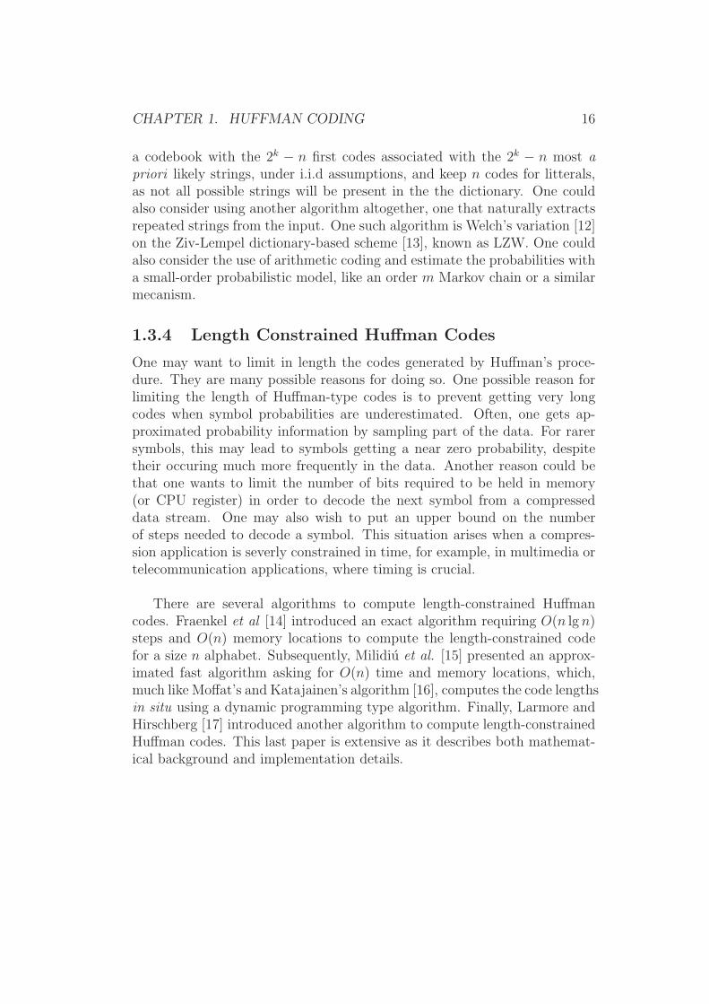
One may want to limit in length the codes generated by Huffman’s proce-dure. They are many possible reasons for doing so. One possible reason forlimiting the length of Huffman-type codes is to prevent getting very longcodes when symbol probabilities are underestimated. Often, one gets ap-proximated probability information by sampling part of the data. For rarersymbols, this may lead to symbols getting a near zero probability, despitetheir occuring much more frequently in the data. Another reason could bethat one wants to limit the number of bits required to be held in memory(or CPU register) in order to decode the next symbol from a compresseddata stream. One may also wish to put an upper bound on the numberof steps needed to decode a symbol. This situation arises when a compres-sion application is severly constrained in time, for example, in multimedia ortelecommunication applications, where timing is crucial.

There are several algorithms to compute length-constrained Huffmancodes. Fraenkel et al [14] introduced an exact algorithm requiring O(n lg n)steps and O(n) memory locations to compute the length-constrained codefor a size n alphabet. Subsequently, Milidiu et al. [15] presented an approx-imated fast algorithm asking for O(n) time and memory locations, which,much like Moffat’s and Katajainen’s algorithm [16], computes the code lengthsin situ using a dynamic programming type algorithm. Finally, Larmore andHirschberg [17] introduced another algorithm to compute length-constrainedHuffman codes. This last paper is extensive as it describes both mathemat-ical background and implementation details.


1.4 Adaptive Huffman Coding

The code generated by the basic Huffman coding algorithm is called the static

Huffman Code. The static Huffman code is generated in two steps. The firststep is the gathering of probability information from the data. This may bedone either by exhaustively scanning the data or by sampling some of it. Ifone opts for exhaustively scanning the data, one may have to deal with largequantities of data, if it is even possible to scan the complete data set at all.In telecommunications, “all the data” does not mean much because the datamay not yet be available as it arrives in small packets from a communicationchannel. If one opts for sampling some of the data, one exposes himself to thepossibility of very bad estimates of the probabilities, yielding an inefficientcode.

Fortunately, there are a number of ways to deal with this problem. Thesolutions bear the common name dynamic or adaptive Huffman coding. Indynamic Huffman coding, we will update the codes as we get better estimatesof the probability, either locally or globally. In this section, we will get alook at the various schemes that have been proposed to achieve adaptivecompression.

1.4.1 Brute Force Adaptive Huffman

One naıve way to do adaptive Huffman coding is the brute force approach.One could recompute the tree each time the probabilities are updated. Aseven an efficient implementation (such as, for example, Moffat’s and Kata-jainen’s astute method [16], Section 1.5) asks for at least O(n) steps, foralphabet size n, it seems impractical to update the codes after each symbol.

What if we compute the new codes every now and then? One could easilyimagine a setting where we recompute the codes only after every k symbolshave been observed. If we update the codes only every 1000 symbols, wedivide the cost of this algorithm by 1000, but we pay in terms of compres-sion efficiency. Another option would be to compute the code only when wedetermine that the codes are significantly out of balance. Such would be thecas when a symbol’s rank in terms of frequency of occurence changes.

This is most easily done with a simple ranking data structure, described


s

Forwardindex

Reversedindex

Frequencyinformation Figure 1.2: A simple structure to

keep symbol rank information. Theforward index uses the symbol di-rectly to find where in the rank tablethe frequency information is stored.The reversed index is used to updatethe forward index when the symbolrank changes up or down.

in Fig. 1.2. A forward index uses the symbol as the key and points at anentry in the table of frequencies. Initially, all the frequencies are set to one(zero could lead to problems). Each time a symbol is observed, we updateits frequency count, stored in the memory location pointed by the forwardindex. The frequency is then bubbled up so as to maintain the array sortedin nonincreasing frequency order. As in bubble sort, we swap the current fre-quency count with the previous while it is larger. We also update the forwardindex by swapping the forward index pointers (we know where they are bythe reversed index). This procedure is expected O(1) amortized times sinceit is unlikely, at least after a good number of observations, that a symbolhas must be bubbled up from the bottom of the array to the top. However,it can be O(n) in the begining when all symbols have a frequency count of1. After, and if, a swap occured in the table we recompute the codes usingany implementation of Huffman’s procedure. Experimental evidence showsthat this algorithms performs slightly better than Vitter’s algorithm (thatwe will see in section 1.4.3) and that the number of tree recomputations islow for text files. Experiments on the Calgary Corpus text files show thatthis algorithm recomputes the tree for about 2-5% of the symbols, giving anacceptable run time even for large files.

This algorithm is not quite as sophisticated as the algorithms we willpresent in the next few subsections. Indeed, it does a lot more work thanseems necessary. With this simple algorithm, we recalculate the whole code-book even when only a few symbols exchange rank. Moreover, exchangingrank does not mean that the symbols also have new code lengths or eventhat they must change codes.


1.4.2 The Faller, Gallager, and Knuth Algorithm

Faller [18] and Gallager [5] independently introduced essentially the samealgorithm, a few years apart. It was later improved upon by Cormack andHorspool [19]. The same improvements appeared again one year later, thistime proposed by Knuth [20]. The adaptive algorithm proposed by Gallagerrequires some introductory material before it is introduced.

A tree has the sibling property if every internal node other than the roothas a sibling and if all nodes can be enumerated in nondecreasing probabilityorder. In such a tree, there are exactly 2n − 2 nodes. A useful theorem in-troduced by Gallager states that a full tree is a Huffman tree if, and only if,it has the sibling property. Let us define the depth of a node as the numberof edges that separate it from the root. The root has a depth of 0. Internalnode probabilities are defined as the sum of the probabilities of the leavesthat they support.

We will maintain a tree such that all nodes at a given depth d havea probability that is less than or equal to all the probabilities of nodes atdepth d − 1 and above. A tree that has this property for all depths is saidto be ordered if the 0-bit goes to the most likely of the two children for eachnode. Furthermore, a tree is said to be lexicographically ordered if, for anydepth d > 1, all the nodes at depth d have smaller probabilities than nodesat depth d−1, and all nodes at depth d can be enumerated in non-decreasingorder, from left to right, in the tree. Finally, a binary prefix code tree is aHuffman tree if, and only if, it is lexicographically ordered.

The update procedure proposed by Gallager requires that the tree re-main lexicographically ordered at all times. We will not discuss how thedata structures are used to maintain efficient access to data within the tree,as Knuth’s paper [20] describes in a complete way a very efficient set of datastructures and sub-algorithms to update the tree.

When a new symbol is observed, its old code (here also obtained by walk-ing down the tree from the root to the leaf that contains this symbol, exactlyas in the basic Huffman algorithm) is transmitted, so that the decoder re-mains synchronized with the encoder. After the code is emitted, the updateprocedure begins. The frequency count associated with the leaf is incre-


mented by one. Let say that this leaf, a, is at depth d. After its count havebeen incremented, we check if all the nodes at depth d are still in nonde-creasing order. If not, we exchange this leaf, with the rightmost node with acount lower than a’s count. Let this node be b. Node b does not have to beat depth d; it can be at depth d−1 or above. After the exchange, we updateb’s parent frequency count recursively up to the root. Since b’s frequency isless than or equal to a’s frequency before the update, no other exchange willbe provoked by the recursive frequency updates. On the other hand, whilewe recursively update a’s ancestors up to the root, we may have to do moreexchanges. Figures 1.3 and 1.4 illustrate the process. The initial state of thetree is adapted from the example given by Gallager in [5].

We have seen that this algorithm takes only positive unit increments onthe frequency count and that it does not deal explicitely with symbols withzero frequency. The problem with only being able to increment the frequencyis that the algorithm captures no local trend in the data, it only convergesslowly on the long-term characteristics of the distribution. Gallager proposesa “frequency decay” method where, every N symbols, all frequencies are mul-tiplied by some constant 0 < α 6 1 to keep them relatively small so that anincrement of 1 has a good chance to provoke an update in the tree. Thereare problems with this method, such as, do we round or truncate the resultafter multiplication by α ? Another problem is how to choose N and α inan adaptive way.

Cormack and Horspool proposed an algorithm to update the frequencyby any positive amount. This procedure was generalized by Knuth to allownegative integers as well. The advantage with negative integer incrementsis that one can keep a size M window overd the source to compress, incre-menting the frequencies according to the symbols that are coming in anddecrementing them according to the symbols that are leaving the window.This method provides a better mechanism to capture non-stationarity in thesource. The hypothesis of stationarity may make sense for certain sources,but not for all. There are many cases where statistics clearly change accord-ing to the source’s history.

Gallager’s algorithm starts with all symbols as leaves and the tree is orig-inally complete. A tree is said to be complete if all leaves lie on at mosttwo different depths. If n, the alphabet size, is of the form n = 2k, then all


leaves are at depth k. Knuth further modified Gallager’s algorithm to includean escape code used to introduce symbols that have not been observed yet.Since it is possible that for a given source, only a subset of the symbols willbe generated for a given message, it is wasteful to allocate the complete treeas soon as compression starts. Knuth’s idea is the following. The tree startsas a single leaf, the special zero-frequency symbol. This leaf will be the spe-cial escape code. When a new symbol is met, we first emit the code for thespecial leaf and then emit the new symbol’s number amongst the remainingunobserved symbols, from 0 to n− r− 1, if r symbols have been observed sofar. This asks for ⌈lg(n − r)⌉ bits. We create the new symbol’s leaf as thesibling of the zero-frequency leaf, creating a parent where the zero frequencyleaf was. This maintains exactly 1 zero frequency leaf at all times. Whenthe last unobserved symbol is encountered, the special zero-frequency leafis simply replaced by this symbol, and the algorithm continues as Gallagerdescribed. The obvious advantage of using this technique is that the codesare very short right from the start.

Knuth gives the complexity of the update and “downdate” (negative in-crement) procedures as being O(− lg P (X = ai)) given we observe symbolai. This gives a total encoding complexity, for a sequence of length m, ofO(mH(X)), since the expected value of − lg P (X = ai) is H(X). This algo-rithm is suitable for adaptive Huffman coding even for low-computational-power environments. The memory requirement is O((2n − 1)c), where c isthe cost (in bytes or bits) of storing the information of a node in memory.

1.4.3 Vitter’s Algorithm: Algorithm Λ

Vitter’s algorithm Λ [21, 22] is a variation of algorithm FGK. The maindifference between algorithm FGK and Vitter’s algorithm Λ is the way thenodes are numbered. Algorithm Λ orders the nodes the same way as al-gorithm FGK, but also asks for leaves of a given weight to always preceedinternal nodes of the same weight and depth, while in algorithm FGK itwas sufficient to order weights of nodes at a given depth from left to right,with no distinction of node type. This modification (as shown in [21]) isenough to guarantee that algorithm Λ encodes a sequence of length s withno more than s bits more than with the static Huffman algorithm, withoutthe expense of transmitting the probability (or code) table to the decoder. In[22], Vitter gives a complete pseudo-Pascal implementation of his algorithm,


a6 5

5 15

20

a5 15

a2 20

20 20

40

40 60

100

a1 3015 15

30

a4 15 a3 15

30 30

60

a)

a6 5

5 15

20

a3 15

a2 20

20 20

40

40 60

101

a1 3015 16

31

a4 15 a5 16

30 31

61

b)

Figure 1.3: A single update. a) shows the tree before the update, b) afterthe observation of symbol a5. The dotted arrow shows where the exchangesoccured.

where most of the data structures introduced in [20] are present. The codeis clear enough that one should not have any major problem translating itto his or her favorite programming language.

1.4.4 Other Adaptive Huffman Coding Algorithms

Jones introduced an algorithm using splay trees [23]. A splay tree is a datastructure where recently accessed nodes are promoted to a position near theroot of the tree [24]. The original splay tree is in fact an ordinary searchtree, with information in every node, and not necessarily full. In the case ofa Huffman-type code tree, the symbols are only in the leaves, and the inter-nal nodes contain no symbol information. Jones presents an algorithm thatmodifies the splay tree algorithm of Tarjan enough so that splaying main-tains a valid Huffman tree. Splaying is also reduced. Instead of promoting asymbol directly to be one of the root’s children, a leaf is allowed to climb onlytwo levels at a time, and depth is reduced by a factor of 2. This algorithmperforms significantly worse that the other adaptive Huffman algorithms inmost cases. Only in most cases, because when the message contains longseries of repeating symbols, the repeated symbol climbs rapidly and quicklygets the shortest code, thus achieving potentially better compression thanthe other algorithms on run-rich data. The splaying provides Jones’ algo-rithm with what we may call short-term memory.


a6 6

6 15

21

a3 15

a2 20

20 21

41

41 61

102

a1 3015 16

31

a4 15 a5 16

30 31

61

a)

a6 6

6 15

21

a3 15

a2 20

20 21

41

41 63

104

a1 3215 16

31

a4 15 a5 16

31 32

63

b)

63

a6 6

6 15

21

a3 15

a2 20

20 21

41

42 63

114

a1 42

15 16

31

a4 15 a5 16

31 41

72

c)

Figure 1.4: After multiple updates. a) shows the tree after the observationof symbol a6. b) shows the tree after two observations of symbol a1. At thispoint, symbol a1 is as far right as it can get on this level, at depth 2. If itis updated again, it will climb at the previous level, depth 1. c) shows theupdated tree after 10 observations of a1. Note that a complete subtree havebeen exchanged, as is shown by the dotted arrow.


Pigeon and Bengio introduced algorithm M where splaying is controlledby a weight rule [25, 26, 27]. A node splays up one level only if it is as heavyas its parent’s sibling. While algorithm Λ almost always beats algorithmM for small alphabets (n = 256), its results are within ≈ 5% of those ofalgorithm Λ on the Calgary Corpus. The situation is reversed when weconsider very large alphabets, say n = 216: Algorithm M beats algorithm Λby ≈ 5% on the Calgary Corpus files treated as composed of 16 bits symbols.This suggests the possible usefulness of algorithm M in the compression ofUnicode files. Another originality of algorithm M is that not all symbols geta leaf. The leaves represent sets of symbols. A set is composed of all thesymbols of the same frequency. The codes are therefore given to frequencyclasses rather than to individual symbols. The complete code is composedof a prefix, the Huffman-like code of the frequency class, and of a suffix, thenumber of the symbol within this frequency class. The suffix is simply thenatural code for the index. The fact that many symbols share the same leafalso cuts down on memory usage. The algorithm produces codes that arenever more than 2 bits longer than the entropy, although in the average case,the average length is very close to the average length produced by the staticHuffman algorithm.

1.4.5 An Observation on Adaptive Algorithms

McIntyre and Pechura [28] advocate the use of static Huffman coding forsmall files or short strings, since the adaptation process needs a relativelylarge number of symbols to be efficient. Furthermore, since the number ofobservations for each symbol is small, it is unlikely that an adaptive algorithmcan produce an efficient codebook. This situation arises when the number ofsymbol to code is large, but still relatively small compared to the alphabetsize. Suppose we want an adaptive code for integers smaller than 216. Onewould expect to have to observe many times the number of symbols in thealphabet before getting a good code. If, on the contrary, the number ofsymbol to code is small, say a few tens, then this code will do much worsethan a static, preoptimized, code. One will then have to consider usingan alternative, such as an adaptive Huffman prefix code, much like thatdiscussed in Section 1.3.2, but where the codes for the equivalence classesare updated by an adaptive algorithm such as algorithm M .


1.5 Efficient Implementations

The work on efficient implementations of Huffman coder/decoder pairs, orcodecs, takes essentially two directions, which are almost mutually exclusive:memory-efficient or speed-efficient. Memory-efficient algorithms vie to saveas much memory as possible in order to have a Huffman codec running withvery little memory. This is achieved by alternative encoding and decodingalgorithms, as much as alternative data structures. Speed-efficient algorithmsare concerned only with the speed of coding or decoding data with a Huffmancodebook. This also relies on alternative data structures, but there is notnecessarily a concern about how much memory is spent.

1.5.1 Memory-Efficient Algorithms

If one opts for an explicit tree representation to maintain the Huffman codeinformation in memory, one has basically few choices. One is a classical bi-nary tree, with three pointers (one for the parent, two for the children), pluspossibly extra information. Another possible choice is to use heap-type stor-age (where the tree is stored in an array organized in a way that the parentfor a node 0 6 k is at k/2, and its children are at 2k + 1 and 2k + 2), butthis kind of storage is potentially sparse because while the Huffman code treeis full, it is rarely complete. Let the reader ponder the amount of memorypotentially wasted by this method.

Moffat and Katajainen [16] proposed a dynamic programming algorithmto compute the lengths of the codes, given that the probabilities are sorted innonincreasing order, in O(n), using O(1) working space, as it overwrites thefrequencies with the lengths as the algorithms progresses. This algorithmsaves working space, especially all the housekeeping data that a list andtree-based algorithm would need. This leads to substancial savings when thenumber of symbols in the alphabet is large. In companion papers, Moffat andTurpin [29, 30] described an algorithm that allows one to use only O(Lmax)memory, using a few tables that describe not the entire tree, but only thedifferent lengths of the codes and their number. Knowing how many codesthere are of a given length is enough to compute the Huffman code of asymbol at encode time. Fortunately, it also works at decode time. The totalmemory needed by this algorithm is O(Lmax) machine words. This algorithmwas also proposed by Hirschberg and Lelewer [31], and it seems that it even


predates this paper!

1.5.2 Speed-Efficient Algorithms

All algorithms presented so far proceed to encoding or decoding one bit at atime. To speed up decoding, Choueka et al. [32], Sieminski [33], and Tanaka[34] introduced various data structures and algorithms, all using the conceptof finite-state automata. While the use of an automaton is not explicit inall papers, the basic idea is that rather than decoding bit by bit, decodingof the input will proceed by chunks of m bits, and the internal state of thedecoder will be repesented as the state of an augmented automaton.

An automaton, in the sense of the theory of computation, is composedof an input alphabet A, a set of states Σ, a set F ⊆ Σ of accepting states,an initial state i, and a transition function T : Σ × A∗ → Σ. The varietyof automata considered here also has an output alphabet Ω, so the transi-tion function becomes T : Σ × A∗ → Σ × Ω∗. The transition function takesas input the current state, a certain number of input symbols, produces acertain number of output symbols, and changes the current state to a newstate. The automaton starts in state i. The automaton is allowed to stop ifthe current state is one of the accepting states in F .

How this applies to fast Huffman decoding is not obvious. In this case,the input alphabet A is 0, 1 and Ω is the original message alphabet. Sincewe are interested in reading m bits at a time, we will have to consider allpossible strings of m bits and all their prefixes and suffixes. For example, letus consider the codebook a → 0, b → 10, c → 11 and a decode block lengthof m = 2. This gives us four possible blocks, 00, 01, 10, 11. Block 00 canbe either aa or the end of b and a; the block 11 either is the end of the codeof c and the begining of b or c; or the code for c, depending on what wasread before this block, what we call the context. The context is maintainedby the automaton in the current state. Knowing the current state and thecurrent input block is enough to unambiguously decode the input. The newstate generated by the transition function will represent the new context,and decoding continues until we reach an accepting state and no more inputsymbols are to be read. Figure 1.5 shows the automaton for the simple code,and Table 1.3 shows its equivalent table form.


00 b

11 c

11 c

10 b

00 aa

01 b

11 c01 a

Figure 1.5: A fast decode automatonfor the code a → 0, b → 10, c → 11.The squiggly arrow indicate the ini-tial state. The accepting state (wherethe decoding is allowed to stop) is cir-cled by a double line. The labels onthe automaton, such as b1b2 → s readas ’on reading b1b2, ouput string s’.

As the reader may guess, the number of states and transitions grows rapi-dely with the number and length of codes, as well as the block size. Speedis gained at the expense of a great amount of memory. We can apply aminimizing algorithm to reduce the size of the automaton, but we still mayhave a great number of states and transitions. We also must consider theconsiderable computation needed to compute the automaton in a minimizedform.

Other authors presented the idea of compressing a binary Huffman codetree to, say, a quaternary tree, effectively reducing by half the depth of thetree. This technique is due to Bassiouni and Mukherjee [35]. They also sug-gest using a fast decoding data structure, which is essentially an automatonby another name. Cheung et al. [36] proposed a fast decoding architec-ture based on a mixture of programmable logic, lookup tables, and softwaregeneration. The good thing about programmable logic is that it can beprogrammed on the fly, so the encoder/decoder can be made optimal withrespect to the source. Current programmable logic technologies are not asfast as current VLSI technologies, but what they lack in speed they have inflexibility.

However, none of these few techniques takes into account the case wherethe Huffman codes are dynamic. Generating an automaton each time thecode adapts is of course computationally prohibitive, even for small messagealphabets. Reconfiguring programmable logic still takes a long time (it takesin the order of seconds), so one cannot consider reprogramming very often.


state read emit goto0 00 aa 0

01 a 110 b 011 c 0

1 00 ba 001 b 110 ca 011 c 1

Table 1.3: The table representation of the automaton of fig. 1.5.

1.6 Conclusion and Further Readings

The literature on Huffman coding is so abundant that an exhaustive list ofpapers, books, and articles is all but impossible to collect. We note a largenumber of papers concerned with efficient implementations, in the contextsof data communications, compressed file systems, archival, and search. Forthat very reason, there are a great number of topics related to Huffman cod-ing that we could not present here, but we can encourage the reader to lookfor more papers and books on this rich topic.

Among the topics we have not discussed is alphabetical coding. An alpha-betical code is a code such that if a preceeds b, noted a ≺ b, in the originalalphabet, then code(a) lexicographically preceeds code(b) when the codes arenot considered as numerical values but as strings of output symbols. Notethat here, lexicographically ordered does not have the same meaning as thatgiven in Section 1.4.2, where we discussed algorithm FGK. This propertyallows, for example, direct comparison of compressed strings. That is, ifaa ≺ ab, then code(aa) ≺ code(ab). Alphabetical codes are therefore suit-able for compressing individual strings in an index or other search table.The reader may want to consult the papers by Gilbert and Moore [37], byYeung [38], and by Hu and Tucker [39], where algorithms to build minimum-redundancy alphabetical codes are presented.

Throughout this chapter, we assumed that all output symbols had anequal cost. Varn presents an algorithm where output symbols are allowed to


have a cost [40]. This situation arises when, say, the communication devicespends more power on some symbols than other. Whether the device usesmany different, but fixed voltage levels, or encodes the signal differentially,as in the LVDS standard, there are symbols that cost more in power to emitthan others. Obviously, we want to minimize both communication time andpower consumption. Varn’s algorithm lets you optimize a code consideringthe relative cost of the output symbols. This is critical for low-powered de-vices such as handheld PDAs, cellular phones, and the like.

In conclusion, let us point out that Huffman codes are rarely used as thesole means of compression. Many, more elaborate, compression algorithmsuse Huffman codes to compress pointers, integers, and other side informationthey need to store efficiently to achieve further compression. One has only tothink of compression algorithms such as the celebrated sliding window Ziv-Lempel technique that encodes both the position and the length of a matchas its mean of compression. Using naıve representations for these quantitiesleads to diminished compression while using Huffman codes give much moresatisfactory results.

Bibliography

[1] S. W. Golomb, “Run length encodings,” IEEE Trans. Inf. Theory,vol. 12, no. 3, pp. 399–401, 1966.

[2] E.R. Fiala and D.H. Greene, “Data compression with finite windows,”Comm. of the ACM, vol. 32, pp. 490–505, April 1989.

[3] D. Huffman, “A method for the construction of minimum redundancycodes,” Proceedings of the I.R.E., vol. 40, pp. 1098–1101, 1952.

[4] R. M. Fano, “The transmission of information,” Tech. Rep. 65, ResearchLaboratory of Electronics, MIT, 1944.

[5] R. G. Gallager, “Variations on a theme by Huffman,” IEEE trans. Inf.

Theory, vol. 24, pp. 668–674, Nov. 1978.

[6] R. M. Capocelli, R. Giancarlo, and I.J. Taneja, “Bounds on the re-dundancy of Huffman codes,” IEEE Trans. Inf. Theory, vol. 32, no. 6,pp. 854–857, 1996.

[7] M. Buro, “On the maximum length of Huffman codes,” Information

Processing Letters, vol. 45, pp. 219–223, 1993.

[8] A. S. E. Campos, “When Fibonacci and Huffman met,” 2000.http://www.arturocampos.com/ac fib Huffman.html.

[9] G. O. H. Katona and T. O. H. Nemetz, “Huffman codes and self-information,” IEEE Trans. Inf. Theory, vol. 22, no. 3, pp. 337–340,1976.

[10] T. C. Bell, J. G. Cleary, and I. H. Witten, Text Compression. Prentice-Hall, 1990. QA76.9 T48B45.

30

BIBLIOGRAPHY 31

[11] B. P. Tunstall, Synthesis of Noiseless Compression Codes. PhD thesis,Georgia Institute of Technology, September 1967.

[12] T. A. Welch, “A technique for high performance data compression,”Computer, pp. 8–19, June 1894.

[13] J. Ziv and A. Lempel, “Compression of individual sequences via variable-rate coding,” IEEE Trans. Inf. Theory, vol. 24, pp. 530–536, September1978.

[14] A. S. Fraenkel and S. T. Klein, “Bounding the depth of search trees,”The Computer Journal, vol. 36, no. 7, pp. 668–678, 1993.

[15] R. L. Milidiu, A. A. Pessoa, and E. S. Laber, “In-place length-restrictedprefix coding,” in String Processing and Information Retrieval, pp. 50–59, 1998.

[16] Alistair Moffat and Jyrki Katajainen, “In place calculation of minimumredundancy codes,” in Proceedings of the Workshop on Algorithms and

Data Structures, pp. 303–402, Springer Verlag, 1995. LNCS 955.

[17] Lawrence L. Larmore and Daniel S. Hirschberg, “A fast algorithm foroptimal length-limited huffman codes,” Journal of the ACM, vol. 37,pp. 464–473, July 1990.

[18] N. Faller, “An adaptive system for data compression,” in Records of the

7th Asilomar Conference on Circuits, Systems & Computers, pp. 393–397, 1973.

[19] Gordon V. Cormack and R. Nigel Horspool, “Algorithms for adaptiveHuffman codes,” Information Processing Letters, vol. 18, pp. 159–165,1984.

[20] D. E. Knuth, “Dynamic Huffman coding,” Journal of Algorithms, vol. 6,pp. 163–180, 1983.

[21] J. S. Vitter, “Design and analysis of dynamic Huffman codes,” Journal

of the ACM, vol. 34, pp. 823–843, October 1987.

[22] J. S. Vitter, “Algorithm 673: Dynamic Huffman coding,” ACM Trans.

Math. Software, vol. 15, pp. 158–167, June 1989.

BIBLIOGRAPHY 32

[23] D. W. Jones, “Application of splay trees to data compression,” Comm.

of the ACM, vol. 31, pp. 996–1007, 1988.

[24] R. E. Tarjan, Data Structures and Network Algorithms. No. 44 in Re-gional Conference Series in Applied Mathematics, SIAM, 1983.

[25] Steven Pigeon and Yoshua Bengio, “A memory-efficient Huffman adap-tive coding algorithm for very large sets of symbols,” Tech. Rep. 1081,Departement d’Informatique et Recherche Operationnelle, Universite deMontreal, 1997.

[26] Steven Pigeon and Yoshua Bengio, “A memory-efficient Huffman adap-tive coding algorithm for very large sets of symbols, revisited,” Tech.Rep. 1095, Departement d’Informatique et Recherche Operationnelle,Universite de Montreal, 1997.

[27] Steven Pigeon and Yoshua Bengio, “Memory-efficient adaptive Huffmancoding,” Doctor Dobb’s Journal, no. 290, pp. 131–135, 1998.

[28] David R. McIntyre and Micheal A. Pechura, “Data compression us-ing static Huffman code-decode tables,” Comm. of the ACM, vol. 28,pp. 612–616, June 1985.

[29] Alistair Moffat and Andrew Turpin, “On the implementation of mini-mum redundancy prefix codes,” IEEE Trans. Comm, vol. 45, pp. 1200–1207, October 1997.

[30] Alistair Moffat and Andrew Turpin, “On the implementation of mini-mum redundancy prefix codes (extended abstract),” in Proceeding of the

Data Compression Conference (M. C. James A. Storer, ed.), pp. 170–179, IEEE Computer Society Press, 1996.

[31] Daniel S. Hirschberg and Debra A. Lelewer, “Efficient decoding of prefixcodes,” Comm. of the ACM, vol. 33, no. 4, pp. 449–459, 1990.

[32] Y. Choueka, S. T. Klein, and Y. Perl, “Efficient variants of Huffmancodes in high level languages,” in Proceedings of the 8th ACM-SIGIR

Conference, Montreal, pp. 122–130, 1985.

[33] A. Sieminski, “Fast decoding of the Huffman codes,” Information Pro-

cessing Letters, vol. 26, pp. 237–241, January 1988.

BIBLIOGRAPHY 33

[34] H. Tanaka, “Data structure of Huffman codes and its application to effi-cient coding and decoding,” IEEE Trans. Inf. Theory, vol. 33, pp. 154–156, January 1987.

[35] Mostafa A. Bassiouni and Amar Mukherjee, “Efficient decoding of com-pressed data,” J. Amer. Soc. Inf. Sci., vol. 46, no. 1, pp. 1–8, 1995.

[36] Gene Cheung, Steve McCanne, and Christos Papadimitriou, “Softwaresynthesis of variable-length code decoder using a mixture of programmedlogic and table lookups,” in Proceeding of the Data Compression Confer-

ence (M. C. James A. Storer, ed.), pp. 121–139, IEEE Computer SocietyPress, 1999.

[37] E.N. Gilbert and E.F. Moore, “Variable length binary encodings,” Bell

Systems Technical Journal, vol. 38, pp. 933–968, 1959.

[38] R. W. Yeung, “Alphabetic codes revisited,” IEEE Trans. Inf. Theory,vol. 37, pp. 564–572, May 1991.

[39] T. C. Hu and A. C. Tucker, “Optimum computer search trees and vari-able length alphabetic codes,” SIAM, vol. 22, pp. 225–234, 1972.

[40] B. Varn, “Optimal variable length codes (arbitrary symbol cost andequal word probability,” Information and Control, vol. 19, pp. 289–301,1971.

Chapter 1 Huﬀman Coding - Steven Pigeonstevenpigeon.com/Publications/publications/Huffman... ·...

Documents

Transcript of Chapter 1 Huﬀman Coding - Steven Pigeonstevenpigeon.com/Publications/publications/Huffman... ·...