Chapter 1 High-Order Discontinuous Galerkin...

September 4, 2010 16:2 World Scientific Review Volume - 9in x 6in dg

Chapter 1

High-Order Discontinuous Galerkin Methods for CFD

Jaime Peraire and Per-Olof Persson

1.1. Introduction

In recent years it has become clear that the current computational methods

for scientific and engineering phenomena are inadequate for many challeng-

ing problems. Examples of these problems are wave propagation, turbulent

fluid flow, as well as problems involving nonlinear interactions and multiple

scales. This has resulted in a significant interest in so-called high-order ac-

curate methods, which have the potential to produce more accurate and re-

liable solutions. A number of high-order numerical methods appropriate for

flow simulation have been proposed, including finite difference methods,1,2

high-order finite volume methods,3,4 stabilized finite element methods,5

Discontinuous Galerkin (DG) methods,6–8 hybridized DG methods,9–11 and

spectral element/difference methods.12,13 All of these methods have advan-

tages in particular situations, but for various reasons most general purpose

commercial-grade simulation tools still use traditional low-order methods.

Much of the current research is devoted to the discontinuous Galerkin

method. This is partly because of its many attractive properties, such

as a rigorous mathematical foundation, the ability to use arbitrary orders

of discretization on general unstructured simplex meshes, and the natural

stability properties for convective-diffusive operators. In this chapter, we

describe our work on efficient DG methods for unsteady compressible flow

applications, including deformable domains and turbulent flows.

1


2 J. Peraire and P.-O. Persson

1.2. Governing Equations

1.2.1. The Compressible Navier-Stokes Equations

The compressible Navier-Stokes equations are written as:

∂ρ

∂t+

∂

∂xi(ρui) = 0, (1.1)

∂

∂t(ρui) +

∂

∂xi(ρuiuj + p) = +

∂τij∂xj

for i = 1, 2, 3, (1.2)

∂

∂t(ρE) +

∂

∂xi(uj(ρE + p)) = − ∂qj

∂xj+

∂

∂xj(ujτij), (1.3)

where ρ is the fluid density, u1, u2, u3 are the velocity components, and E

is the total energy. The viscous stress tensor and heat flux are given by

τij = µ

(

∂ui∂xj

+∂uj∂xi− 2

3

∂uk∂xj

δij

)

, (1.4)

and

qj = −µ

Pr

∂

∂xj

(

E +p

ρ− 1

2ukuk

)

. (1.5)

Here, µ is the viscosity coefficient and Pr = 0.72 is the Prandtl number

which we assume to be constant. For an ideal gas, the pressure p has the

form

p = (γ − 1)ρ

(

E − 1

2ukuj

)

, (1.6)

where γ is the adiabatic gas constant.

1.2.2. Turbulence Modeling

We consider two different approaches for the simulation of turbulent flows –

Implicit Large Eddy Simulation (ILES) and the Reynolds Averaged Navier-

Stokes (RANS) equations.

In LES modeling, the large scale flow features are resolved while the

small scales are modeled. The rationale behind this is that the small scales

are isotropic, carry less of the flow energy and therefore do not have as

much influence on the mean flow, and can therefore be approximated or

modeled. The effect of these subgrid scales (SGS) is approximated by an

eddy viscosity which can be derived from a so-called SGS model or can

be taken to be equal to the dissipation in the numerical scheme, which is

the principle behind the ILES model.14 Simulations based on ILES models


High-Order Discontinuous Galerkin Methods for CFD 3

often give very accurate predictions but are limited to low Reynolds number

flows because of the high computational cost of resolving the large scale

features of the flow.

For the RANS modeling, we add a turbulent dynamic (or eddy) vis-

cosity µt to µ in the Navier-Stokes equations (1.1)-(1.3), and solve for the

time-averaged values of the flow quantities ρ, ρui, and ρE. We use the

Spalart-Allmaras One-Equation model for µt,15 where a working variable ν

is introduced to evaluate the turbulent dynamic viscosity. This new variable

obeys the transport equation

Dν

Dt= cb1Sν +

1

σ

[

∇ · ((ν + ν)∇ν) + cb2 (∇ν)2]

− cw1fw

[

ν

d

]2

. (1.7)

For simplicity, the trip terms have been excluded here, meaning that we

assume that the Reynolds numbers are large enough so that the flow over

the entire body surface is turbulent. The turbulent dynamic viscosity is

then calculated as

µt = ρνt , νt = νfv1 , fv1 =χ3

χ3 + c3v1, χ =

ν

ν. (1.8)

The production term is expressed as

S = S +ν

κ2d2fv2 , S =

√

2ΩijΩij , fv2 = 1− χ

1 + χfv1. (1.9)

Here Ωij =12 (∂ui/∂xj−∂uj/∂xi) is the rotation tensor and d is the distance

from the closest wall. The function fw is given by

fw = g

[

1 + c6w3

g6 + c6w3

]1/6

, g = r + cw2(r6 − r) , r =

ν

Sκ2d2. (1.10)

The closure constants used here are cb1 = 0.1355, cb2 = 0.622, cv1 = 7.1,

σ = 2/3, cw1 = (cb1/κ2) + ((1 + cb2)/σ), cw2 = 0.3, cw3 = 2, κ = 0.41.

1.2.3. Mapping-based ALE Formulation for Deformable Do-

mains

Here, we formulate the Navier-Stokes equations in an Arbitrary-Lagrangian

Eulerian (ALE) framework, to allow for variable geometries.16 We follow a

similar approach to that presented in Ref. 2. That is, we construct a time

dependent mapping between a fixed reference domain and the time vary-

ing physical domain. The original equations in the Eulerian domain are

then transformed to the fixed reference configuration and the discretization



is always carried out on the fixed domain. In order to ensure that con-

stant solutions in the physical domain are preserved exactly, we introduce

an additional scalar equation in which the Jacobian of the transformation

is integrated numerically using the same spatial and time discretization

schemes. This numerically integrated Jacobian is used to correct for inte-

gration errors in the conservation equations.

1.2.3.1. The Mapping

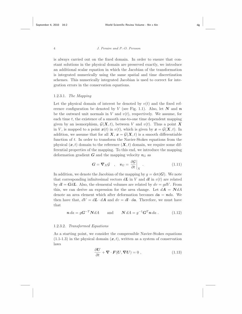
Let the physical domain of interest be denoted by v(t) and the fixed ref-

erence configuration be denoted by V (see Fig. 1.1). Also, let N and n

be the outward unit normals in V and v(t), respectively. We assume, for

each time t, the existence of a smooth one-to-one time dependent mapping

given by an isomorphism, G(X, t), between V and v(t). Thus a point X

in V , is mapped to a point x(t) in v(t), which is given by x = G(X, t). In

addition, we assume that for all X, x = G(X, t) is a smooth differentiable

function of t. In order to transform the Navier-Stokes equations from the

physical (x, t) domain to the reference (X, t) domain, we require some dif-

ferential properties of the mapping. To this end, we introduce the mapping

deformation gradient G and the mapping velocity vG as

G = ∇XG , vG =∂G∂t

∣

∣

∣

∣

X

. (1.11)

In addition, we denote the Jacobian of the mapping by g = det(G). We note

that corresponding infinitesimal vectors dL in V and dl in v(t) are related

by dl = GdL. Also, the elemental volumes are related by dv = gdV . From

this, we can derive an expression for the area change. Let dA = NdA

denote an area element which after deformation becomes da = nda. We

then have that, dV = dL · dA and dv = dl · da. Therefore, we must have

that

n da = gG−TNdA and N dA = g−1GTn da . (1.12)

1.2.3.2. Transformed Equations

As a starting point, we consider the compressible Navier-Stokes equations

(1.1-1.3) in the physical domain (x, t), written as a system of conservation

laws

∂U

∂t+∇ · F (U ,∇U) = 0 , (1.13)



X1

X2

NdA

V

x1

x2

nda

vG , g, vG

Fig. 1.1. Mapping between the physical and the reference domains.

where U is the vector of conserved variables and F is a generalized column

flux vector which components are the physical flux vectors in each of the

spatial coordinate directions. Here F incorporates both inviscid and viscous

contributions. That is, F = F inv(U)+F vis(U ,∇U) and ∇ represents the

spatial gradient operator in the x variables.

In order to obtain the corresponding conservation law written in the

reference configuration we re-write the above equation in an integral form

as∫

v(t)

∂U

∂tdv +

∫

∂v

F · n da = 0. (1.14)

Note that the above expression follows directly from (1.13) by integrating

over v(t) and applying the divergence theorem. It is now possible to utilize

the mapping and evaluate these integrals in the reference configuration.

Consider first the second term,∫

∂v

F · n da =

∫

∂V

F · (gG−TN) dA =

∫

∂V

(gG−1F ) ·N dA. (1.15)

Similarly, the first integral is transformed by means of Reynolds transport

theorem to give∫

v(t)

∂U

∂tdv =

d

dt

∫

v(t)

U dv −∫

∂v

(UvG) · n da (1.16)

=d

dt

∫

V

g−1U dV −∫

∂V

(UvG) · (gG−TN) dA (1.17)

=

∫

V

∂(g−1U)

∂t

∣

∣

∣

∣

X

dV −∫

∂V

(gUG−1vG) ·N dA . (1.18)



Using the divergence theorem once again enables an equivalent local con-

servation law in the reference domain to be derived as,

∂UX

∂t

∣

∣

∣

∣

X

+∇X · FX(UX ,∇XUX) = 0 , (1.19)

where the time derivative is at a constant X and the spatial derivatives are

taken with respect to the X variables. The transformed vector of conserved

quantities and corresponding fluxes in the reference space are

UX = gU , (1.20)

FX = gG−1F −UXG−1vG , (1.21)

or, more explicitly,

FX = F invX + F vis

X , (1.22)

F invX = gG−1F inv −UXG−1vG , (1.23)

F visX = gG−1F vis , (1.24)

and by a simple application of the chain rule,

∇U = ∇X(g−1UX)G−1 = (g−1∇XUX +UX∇X(g−1))G−1 . (1.25)

1.2.3.3. Geometric Conservation Law

It turns out that, for arbitrary mappings, a constant solution in the physical

domain is not necessarily a solution of the discretized equations in the ref-

erence domain. Even though this error is typically very small for high order

discretizations, the situation is quite severe for lower order approximations

since the free-stream condition is not preserved identically. Satisfaction of

the constant solution is often referred to as the Geometric Conservation

Law (GCL) and is was originally discussed in Ref. 17. The source of the

problem is the inexact integration of the Jacobian g of the transformation

by the numerical scheme.

First, we note that using expressions (1.12) together with the divergence

theorem, it is straightforward to prove the so-called Piola relationships,

which hold for arbitrary vectors W and w:

∇X ·W = g∇ · (g−1GW ) , ∇ ·w = g−1∇X · (gG−1w) . (1.26)

When the solution U is constant, say U , we have

∇X · FX = g∇ · (F − UvG) = −gU∇ · vG = −[∇X · (gG−1vG)]U .

(1.27)



Therefore, for a constant solution U , equation (1.19) becomes

∂UX

∂t

∣

∣

∣

∣

X

+∇X · FX = g−1Ux

(

∂g

∂t

∣

∣

∣

∣

X

−∇X · (gG−1vG)

)

. (1.28)

We see that the right hand side is only zero if the equation for the time

evolution of the transformation Jacobian g

∂g

∂t

∣

∣

∣

∣

X

−∇X · (gG−1vG) = 0 , (1.29)

is integrated exactly by our numerical scheme. Since in general, this will

not be the case, the constant solution Ux in the physical space will not be

preserved exactly.

An analogous problem was brought up in the formulation presented in

Ref. 2. The solution proposed there was to add some corrections aimed

at canceling the time integration errors. Here, we use a slightly different

approach. The system of conservation laws (1.19) is replaced by

∂(gg−1UX)

∂t

∣

∣

∣

∣

X

−∇X · FX = 0 , (1.30)

where g is obtained by solving the following equation

∂g

∂t

∣

∣

∣

∣

X

−∇X · (gG−1vG) = 0 . (1.31)

We note that even though g is an approximation to g, when the above

equation is solved numerically with the same numerical scheme employed

for (1.30), its value will differ from that of g due to integration errors.

It is straightforward to verify that (1.30) does indeed preserve a constant

solution as desired. Finally, we point out that the fluxes in equation (1.31)

do not depend on U and are only a function of the mapping. This has

two implications. First, when the mapping is prescribed, equation (1.31)

can be integrated independently to obtain g in time. Second, the fluxes in

(1.31) do not require communication with the neighboring elements, thus

simplifying its numerical solution.



1.3. Numerical Methods

1.3.1. The Compact Discontinuous Galerkin Method

In order to develop a Discontinuous Galerkin method, we consider a general

system of conservation laws

∂u

∂t+∇ · F inv(u) = ∇ · F vis(u,∇u) + S(u,∇u) , (1.32)

in a domain Ω, with conserved state variables u, inviscid flux function F inv,

viscous flux function F vis and source term S. We note that the governing

equations described in the previous section can all be cast in this particular

form. We eliminate the second order spatial derivatives of u by introducing

additional variables q = ∇u:∂u

∂t+∇ · F inv(u) = ∇ · F vis(u, q) + S(u, q) , (1.33)

q −∇u = 0 . (1.34)

Next, we consider a triangulation Th of the spatial domain Ω and introduce

the finite element spaces Vh and Σh as

Vh = v ∈ [L2(Ω)]m | v|K ∈ [Pp(K)]m, ∀K ∈ Th , (1.35)

Σh = r ∈ [L2(Ω)]dm | r|K ∈ [Pp(K)]dm, ∀K ∈ Th , (1.36)

where Pp(K) is the space of polynomial functions of degree at most p ≥ 0

on triangle K, m is the dimension of u and d is the spatial dimension. We

now consider DG formulations of the form: find uh ∈ Vh and qh ∈ Σh such

that for all K ∈ Th, we have∫

K

qh · r dx = −∫

K

uh∇ · r dx+

∫

∂K

ur · nds,

∀r ∈ [Pp(K)]dm , (1.37)∫

K

∂uh∂t

v dx−∫

K

F inv(uh) · ∇v dx+

∫

∂K

F invv ds =

−∫

K

F vis(uh, qh) · ∇v dx+

∫

∂K

F visv ds+

∫

K

S(uh, qh)v dx,

∀v ∈ [Pp(K)]m . (1.38)

Here, the numerical fluxes F inv, F vis and u are approximations to F inv ·n,F vis · n and u, respectively, on the boundary ∂K of the element K and n

is the unit normal to the boundary. As commonly done, the inviscid fluxes

F inv are approximated using an approximate Riemann solver. In most of



our applications, we use the method due to Roe18. For the viscous fluxes

F vis, we use the compact discontinuous Galerkin (CDG) scheme.19

The CDG scheme consists of a modification of the original Local Dis-

continuous Galerkin method.20 This modification is aimed at making the

scheme more compact and hence more attractive computationally, espe-

cially when dealing with implicit discretizations and implementations on

parallel computers. In order to describe the CDG method, we first con-

sider the LDG method for approximating F vis. In the LDG method, we

choose u and F vis according to

F vis = F vis(uh, qh) · n+ C11[[uhn]] +C12[[Fvis(uh, qh) · n]] (1.39)

u = uh −C12 · [[uhn]] . (1.40)

Here, and [[ ]] denote the average and jump operators across the inter-

face.19 The constant C11 can be chosen equal to zero, except at the bound-

ary interfaces, leading to the so called minimum dissipation scheme.21 On

the other hand, C12 is chosen as C12 = n∗, where n∗ is the unit normal to

the interface taken with an arbitrary sign. The only constraint on the sign

is that all the C12 vectors corresponding to the different faces of a given

element do not all point either inwards or outwards. See Refs. 19,20 for

additional details.

One of the major drawbacks of the LDG method is that it results in

a scheme which is non-compact. This means that in the Jacobian of the

residual some elements are not only connected to their neighbors but to

the neighbors of its neighbors. This situation arises when structured or

unstructured meshes are used as discussed in Ref. 19.

In the CDG method, equation (1.39) is replaced by

(F vis)e = F vis(uh, qeh) · n+ C11[[uhn]] +C12[[F

vis(uh, qeh) · n]] . (1.41)

The “edge” fluxes qeh are computed by solving the equation∫

K

qeh · r dx = −∫

K

uh∇ · r dx+

∫

∂K

uer · nds, ∀r ∈ [Pp(K)]dm , (1.42)

where

ueh =

uh on edge e, given by equation (1.40),

uh otherwise.(1.43)

The CDG scheme is a little more expensive than the original LDG method

as it requires a different elemental value of qeh for each edge (or face) e of

the element, but it results in a scheme with a sparser structure than the



LDG method and element-wise compact connectivities. For more details

we refer to Ref. 19.

1.3.2. Stabilization by Artificial Diffusion

Discontinuities and other under-resolved solution features pose consider-

able difficulties for most high-order methods. Several approaches inspired

by the finite volume methodology have been proposed. The most straight-

forward approach consists of using some form of shock sensing to identify

the elements lying in the shock region and reducing the order of the inter-

polating polynomial there.22,23 Despite its simplicity, this approach may

yield satisfactory answers, in particular when combined with adaptive mesh

refinement procedures.

More sophisticated approaches exist for selecting the interpolating poly-

nomial such as those based on weighted essentially non-oscillatory (WENO)

concepts.7,24,25 These methods allow for stable discretizations near discon-

tinuities while still maintaining a high-order approximation. Although these

methods have several attractive features, they have not yet been demon-

strated in the practical unstructured mesh context using high-order ap-

proximation polynomials. Other interesting alternatives are based on ap-

plying filters to the solution,26,27 the selective application of viscosity to

the different spectral scales,28 and methods based on reconstructing the

solution from unlimited oscillatory solutions computed using a high-order

method.29,30 These methods hold the promise of yielding uniformly ac-

curate solutions near the discontinuity in a pointwise sense. However, a

number of issues still remain unresolved. In particular, the extension of

these methods to multiple dimensions is an open question.

In Ref. 31, we proposed a new strategy inspired by the early artificial

viscosity methods,32 which has proved to be surprisingly effective in the

context of high-order DG methods.33–35 The rationale behind the method

is to add viscosity to the original equations in order to spread discontinu-

ities over a length scale that can be adequately resolved within the space

of approximating functions. The goal is not to introduce discontinuities

in the approximating space, but to resolve the sharp gradients existing in

a viscous shock with continuous approximations. For low order approxi-

mations, such as piecewise constant and/or linear, this approach produces

discontinuities which are spread over several cells (e.g. 2-4 cells). There-

fore, it is considered to be inferior to the more established finite volume

shock capturing approaches. This is because several cells are required to



resolve a viscous shock profile with piecewise linear approximations.

However, for higher order polynomial approximations, the situation is

different. The resolution of a piecewise polynomial of order p scales like

δ ∼ h/p. This means that the amount of artificial viscosity required to

resolve a shock profile is O(h/p). Keeping h fixed, the amount of artificial

viscosity required scales like 1/p and the accuracy of the solution in the

neighborhood of the shock becomes O(h/p). This compares favorably to

the more standard approaches which are only O(h) accurate. In other

words, for high order p, we can exploit sub-cell resolution and obtain shock

profiles which are much thinner than the element size. Recall that in the

more standard approaches, the order of the interpolating polynomial is

reduced over the whole element and as a consequence, there is no hope for

resolving the shock profile at a sub-cell level.

1.3.2.1. Artificial Viscosity Models

The most straight-forward artificial viscosity model is to add Laplacian

diffusion to the system of conservation laws

∂u

∂t+∇ · F (u,∇u) = ∇ · (ε∇u). (1.44)

Here, the parameter ε controls the amount of viscosity. The shocks that may

appear in the solution to this modified equation will spread over layers of

thickness O(ε). Therefore, when attempting to approximate these solutions

numerically, ε should be chosen as a function of the resolution available in

the approximating space. Near the shocks, we take ε = O(h/p), where h is

the element size and p is the order of the approximating polynomial. Away

from discontinuities, where the unmodified solution is resolved, we want

ε = 0.

Instead of the Laplacian term added to the right hand side of equation

(1.44), one can also consider a physically inspired artificial viscosity term

analogous to dissipative terms in the Navier-Stokes equations but with a

viscosity coefficient which is determined by numerical considerations. De-

tails about this physically inspired model can be found in Ref. 31. In our

experience, the physical model and the Laplacian model of equation (1.44)

perform similarly.

1.3.2.2. Discontinuity Sensor

In order to avoid the use of artificial viscosity in resolved regions of the

flow, we utilize a resolution sensor. We write the solution within each el-



ement in terms of a hierarchical family of orthogonal polynomials. In 1D,

the solution is represented by an expansion in terms of orthonormal Legen-

dre polynomials, whereas in multidimensions, an orthonormal Koornwinder

basis36 is employed within each triangle. For smooth solutions, the coeffi-

cients in the expansion are expected to decay very quickly. On the other

hand, when the solution is not smooth, the strength of the discontinuity

will dictate the rate of decay of the expansion coefficients. We express the

solution of order p within each element in terms of an orthogonal basis as

u =

N(p)∑

i=1

uiψi , (1.45)

where N(p) is the total number of terms in the expansion and ψi are the

basis functions. In addition, we also consider a truncated expansion of the

same solution, only containing the terms up to order p− 1, that is,

u =

N(p−1)∑

i=1

uiψi . (1.46)

Within each element Ωe, the following resolution indicator is defined,

Se =(u− u, u− u)e

(u, u)e, (1.47)

where (·, ·)e is the standard inner product in L2(Ωe). In practice, we have

found Se to be a remarkably reliable indicator

Once the shock has been sensed, the amount of viscosity is taken to

be constant over each element and determined by the following smooth

function,

εe =

0 if se < s0 − κ ,ε02

(

1 + sin π(se−s0)2κ

)

if s0 − κ ≤ se ≤ s0 + κ ,

ε0 if se > s0 + κ .

(1.48)

Here, se = log10 Se and the parameters ε0 ∼ h/p, s0 ∼ 1/p4, and κ are

chosen empirically sufficiently large so as to obtain a sharp but smooth

shock profile.

1.3.3. Parallel Preconditioned Newton-Krylov Solvers

After discretization of (1.32) using the Compact Discontinuous Galerkin

method and elimination of the variables associated with qh within each el-

ement, we obtain system of coupled ordinary differential equations (ODEs)



of the form:

Mu = r(u) , (1.49)

where u(t) is a vector containing the degrees of freedom associated with

uh, which is represented using a nodal basis. The vector u denotes the

time derivative of u(t), M is the mass matrix, and r is the residual vec-

tor. We integrate (1.49) implicitly in time using either diagonal implicit

Runge-Kutta methods (DIRK)37 or the backward differentiation formulas

(BDF).38 Using Newton’s method for solving the nonlinear systems of equa-

tions that arise, it is required to solve linear systems involving matrices of

the form

A ≡ α0M −∆tdr

du≡ α0M −∆tK . (1.50)

For simplicity of presentation, we assume that α0 = 1, which is the case

for the first-order accurate backward Euler method. Other values of α0,

as required for higher-order methods, simply correspond to a scaling of the

timestep ∆t.

1.3.3.1. Jacobian Sparsity Pattern

The system matrix A = M − ∆tK is sparse with a block-wise structure

corresponding to the element connectivities. An example of a small trian-

gular mesh with polynomial degrees p = 2 within each element is shown in

Fig. 1.2. It is worth pointing out that the number of nonzero blocks in each

row is equal to four in 2D and five in 3D, except for boundary elements.

To be able to use machine optimized dense linear algebra routines, such as

the BLAS/LAPACK libraries,39 we represent A in an efficient dense block

format, see Ref. 40 for details. We note that our CDG scheme actually

produces sparser off-diagonal blocks than other known methods,19 which

we take advantage of in our implementation. However, in what follows, we

assume for simplicity that all nonzero blocks are full dense matrices. The

block with element indices 1 ≤ i, j ≤ n will be denoted by Aij , with n the

total number of elements.

1.3.3.2. Incomplete LU Preconditioning

It is clear that the performance of the iterative solvers will depend strongly

on the timestep ∆t. As ∆t → 0, the matrix A reduces to the mass ma-

trix, which is block diagonal and inverted exactly by all preconditioners

that we consider. However, as ∆t → ∞, the problem becomes harder and



Fig. 1.2. An example mesh with elements of polynomial order p = 2, and the corre-

sponding block matrix for a scalar problem.

often not well-behaved. Physically, a small ∆t means that the informa-

tion propagation is local, while a large ∆t means information is exchanged

over large distances during the timestep. This effect, which is important

when designing iterative methods, is even more important when we consider

parallel algorithms since algorithms based on local information exchanges

usually scale better than ones with global communication patterns.

When solving the system Au = b using Krylov subspace iterative meth-

ods such as GMRES, it is essential to use a good preconditioner. This

amounts to finding an approximation A to A which allows for a rela-

tively inexpensive computation of A−1p for arbitrary vectors p. One of

the simplest choices that performs reasonably for many problems is the

block-diagonal, or the block-Jacobi, preconditioner

AJij =

Aij if i = j ,

0 if i 6= j .(1.51)

Clearly, AJ is cheap to invert compared to A, since all the diagonal blocks

are independent. However, unlike the point-Jacobi iteration, there is a

significant preprocessing cost in the factorizations of the diagonal blocks

AJij , which is comparable to the cost of more complex factorizations.40

A minor modification of the block-diagonal preconditioner is the block

Gauss-Seidel preconditioner, which keeps the diagonal blocks plus all the

upper triangular blocks:

AGSij =

Aij if i ≤ j ,0 if i > j .

(1.52)



The preprocessing cost is the same as before, and solving AGSu = p is only

a constant factor more expensive than for AJ . The Gauss-Seidel precondi-

tioner can perform well for some simple problems, such as scalar convection

problems, but in general it only gives a small factor of improvement over

the block-diagonal preconditioner. Furthermore, the sequential nature of

the triangular back-solve with AGS makes the Gauss-Seidel preconditioner

hard to parallelize.

A more ambitious preconditioner with similar storage and computa-

tional cost is the block incomplete LU factorization AILU = LU with zero

fill-in. This block-ILU(0) algorithm corresponds to block-wise Gaussian

elimination, where no new blocks are allowed into the matrix. This factor-

ization can be computed with the following simple algorithm:

function [L, U ] ← IncompleteLU (A, mesh)

U = A, L = I

for j = 1, . . . , n− 1

for neighbors i > j of j in mesh

Lij = UijU−1jj

Uii = Uii − LikUki

We also note here that the upper-triangular blocks of U are identical

to those in A, which reduces the storage requirements for the factoriza-

tion. The back-solve using L and U has the same sequential nature as for

Gauss-Seidel, but it turns out that the performance of the block-ILU(0)

preconditioner can be fundamentally better.

1.3.3.3. Minimum Discarded Fill Element Ordering

It is clear that the Gauss-Seidel and the incomplete LU factorizations will

depend strongly on the ordering of the blocks, or the elements, in the mesh.

This is because of the mesh ordering determines which element connections

are kept and which are discarded when calculating A. In Refs. 40,41, we

proposed a simple heuristic algorithm for finding appropriate element or-

derings. Our algorithm considers the fill that would be ignored if element

j′ was chosen as the pivot element at step j:

∆U(j,j′)ik = −Uij′U

−1j′j′Uj′k, for neighbors i ≥ j, k ≥ j of element j′.

(1.53)



The matrix ∆U (j,j′) corresponds to fill that would be discarded by the

ILU algorithm. In order to minimize these errors, we consider a set of

candidate pivots j′ ≥ j and pick the one that produces the smallest fill. As

a measurement of the magnitude of the fill, or the corresponding weight,

we take the Frobenius matrix norm of the fill matrix:

w(j,j′) = ‖∆U (j,j′)‖F . (1.54)

As a further simplification, we note that

‖∆U(j,j′)ik ‖F = ‖ − Uij′U

−1j′j′Uj′k‖F ≤ ‖Uij′‖F‖U−1

j′j′Uj′k‖F , (1.55)

which means we can estimate the weight by simply multiplying the norms of

the individual matrix blocks. By pre-multiplication of the block-diagonal,

we can also avoid the matrix factor U−1j′j′ above. See Ref. 41 for full pseudo-

code of the algorithm.

We note that for a pure upwinded scalar convective problem, the MDF

ordering is optimal since at each step it picks an element that either does

not affect any other elements (downwind) or does not depend on any other

elements (upwind), resulting in a perfect factorization. But the algorithm

works well for other problems too, including multivariate and viscous prob-

lems, since it tries to minimize the error between the exact and the ap-

proximate LU factorizations. It also takes into account the effect of the

discretization (e.g. highly anisotropic elements) on the ordering. These

aspects are harder to account for with methods that are based on physical

observations, such as line-based orderings.42–45

1.3.3.4. Coarse Scale Corrections and the ILU/Coarse Scale Pre-

conditioner

Multi-level methods, such as multigrid46 solve the system Au = b by in-

troducing coarser level discretizations. This coarser discretization can be

obtained either by using a coarser mesh (h-multigrid) or, for high-order

methods, by reducing the polynomial degree (p-multigrid43,47). The resid-

ual is restricted to the coarse scale where an approximate error is computed,

which is then applied as a correction to the fine scale solution. A few itera-

tions of a smoother (such as Jacobi’s method) are applied after and possibly

before the correction to reduce the high-frequency errors.

For our DG discretizations, it is natural and practical to consider coarser

scales obtained by reducing the polynomial order p. The problem size is

highly reduced by decreasing the polynomial order to p = 0 or p = 1, even



from moderately high orders such as p = 4. For very large problems it may

be necessary to consider h-multigrid approaches to solve the coarse grid

problem, but here we only use p-multigrid.

Furthermore, we have observed that we often get overall better perfor-

mance by using a simple two-level scheme where the fine level corresponds

to p = 4 and the coarse level is either p = 1 or p = 0 rather than a hierar-

chy of levels. Thus, our preconditioning algorithm solves the linear system

Au = b approximately using a single coarse scale correction,

0. A(0) = P TAP Precompute coarse operator, block wise

1. b(0) = P T b Restrict residual element/component wise

2. A(0)u(0) = b(0) Solve coarse scale problem

3. u = Pu(0) Prolongate solution element/component wise

4. u = u+αA−1(b−Au) Apply smoother A with damping α

Possible smoothers A include block Jacobi AJ or Gauss-Seidel AGS. It is

also known that an ILU0 factorization can be used as a smoother for multi-

grid methods,48,49 and it has been reported that it performs well for the

Navier-Stokes equations, at least in the incompressible case using low-order

discretizations.50 Inspired by this, we use the block ILU0 factorization AILU

as a post-smoother for a two-level scheme. Our numerical experiments in-

dicate that the block ILU0 preconditioner and the low-degree correction

preconditioner complement each other. With our MDF element ordering

algorithm, the ILU0 performs almost optimally for highly convective prob-

lems, while the coarse scale correction with either block diagonal, block GS,

or block ILU0 post-smoothing, performs very well in the diffusive limit.

The restriction/prolongation operator P is a block diagonal matrix with

all the blocks being identical. The prolongation operator has the effect of

transforming the solution from nodal basis to a hierarchical orthogonal basis

function based on Koornwinder polynomials36 and setting the coefficients

corresponding to the higher modes equal to zero. The transpose of this

operator is used for the restriction of the weighted residual and for the

projection of the matrix blocks. For more details on these operators we

refer to Ref. 51. We use a smoothing factor α = 1 for the ILU0 smoother.

We use a direct sparse solve for the linear system in step 2, and we note

that the matrix A(0) is usually magnitudes smaller than A.



Fig. 1.3. Partitioning of the mesh elements.

1.3.3.5. Parallelization

The domain is naturally partitioned by the elements to achieve load bal-

ancing and low communication volumes, see Fig. 1.3. Because of the

element-wise compact stencil of the CDG scheme, only one additional layer

of elements has to be maintained for each process in addition to the el-

ements in the partition. The elements at the domain boundary are pro-

cessed first, then the computed data is sent to neighboring processes using

non-interrupting communications, and while the data is sent the interior

elements are processed. This typically leads to algorithms where the com-

munication costs are negligible for evaluations of the residual r(u), and

therefore also for explicit time integration methods, as well as for the eval-

uation of the Jacobian matrix K = ∂r/∂u.

In the iterative implicit solvers, the matrix-vector products also scale

well in terms of communication, by overlapping with the computation of

the interior elements. However, a problem here is the fact that the matrix-

vector product operations are highly memory intensive, and tend to give

poor scaling on multicore processors. Another issue is the parallelization of

the preconditioner, where in particular the Gauss-Seidel and the incomplete

LU preconditioners have a highly serial structure that is hard to parallelize.

Our preferred approach for parallelization of the ILU factorization is

to apply it according to the element orderings determined by the MDF

algorithm, but ignoring any contributions between elements in different

partitions. In standard domain decomposition terminology, this essentially

amounts to a non-overlapping Schwartz algorithm with incomplete solu-

tions.52 It is clear that this approach will scale well in parallel, since each

process will compute a partition-wise ILU factorization independent of all



other processes.

To minimize the error introduced by separating the ILU factorizations,

we use the ideas from the MDF algorithm to obtain information about

the weights of the connectivities between the elements. By computing a

weighted partitioning using the weight

Cij = ‖A−1ii Aij‖F (1.56)

between element i and j, we obtain partitions that are less dependent on

each other, and reduce the error from the decomposition. The drawback is

that the total communication volume might be increased, but if desired, a

trade-off between these two effects can be obtained by adding a constant

C0 to the weights. In practice, since the METIS software53 used for the

partitioning requires integer weights, we scale and round the Cij values to

integers between 1 and 100. It is clear that this method reduces to the

block-Jacobi method as the number of partitions approaches the number of

elements. However, in any practical setting, each partition will have at least

100’s of elements, in which the difference between partition-wise block-ILU

and block-Jacobi is quite significant.

1.4. Applications

In this section we present four representative applications of our high-order

DG methods.

1.4.1. Aeroacoustics and Kelvin-Helmholtz Instability

Our first example, which is adapted from Ref. 54, is an aeroacoustics prob-

lem with nonlinear interactions between a long-range wave and small-scale

flow features. The flow has a Mach number of M = 1/20 in the double-

periodic rectangular domain −L ≤ x ≤ L = 1/M = 20, 0 ≤ y ≤ 2L/5 = 8.

We use a Cartesian grid of 400-by-80 quadrilateral elements, with each ele-

ment split into two triangles, giving a total of 64,000 elements. Within each

elements we use polynomials of degree p = 3, giving a total of 640,000 DOFs

per component, or 2.56 million DOFs for the compressible Navier-Stokes

equations.

The initial conditions are based on a sawtooth-shaped density profile,

which we smooth to allow an accurate high-order representation on the

grid:

Φ(y) =y

10− 2

5(erf(δ(y − L/5))− 1), (1.57)



Fig. 1.4. The acoustic Kelvin-Helmholtz problem at three time instances, with colorrepresenting the density. The initially long-range acoustic wave forms a weak shock,which interacts with the density stratified flow to produce shear instabilities.

with grid resolution δ = N/p = 80/3. We also define the long-range acoustic

wave shape by

Ψ(x) = 1 + cosπx

L. (1.58)

The initial density, pressure, and velocities are then

ρ = 1 + 0.2MΨ(x) + Φ(y), u =√γΨ(x), (1.59)

p = (1 + γMΨ(x))/M2, v = 0, (1.60)

with γ = 1.4. We solve the compressible Navier-Stokes equations, with

a dynamic viscosity coefficient µ = 1/160, corresponding to a Reynolds

number Re = 6, 400 based on the length of the domain. Since the grid is

uniform and we wish to resolve the acoustic waves time-accurately, we use

a standard explicit RK4 time integrator with timestep ∆t = 1.25 · 10−4.

The resulting flow field is shown in Fig. 1.4, as color plots of the density

at three time instances t = 2.5, t = 7.5, and t = 12.5. We note that the

acoustic wave deforms into a weak shock, and that the density jump causes

a Kelvin-Helmholtz type instability at the interface. Furthermore, although

not clearly visible from these figures, there are highly complex interactions

between the waves and the flow features, and capturing these accurately is

one of our main motivations for using high-order methods.



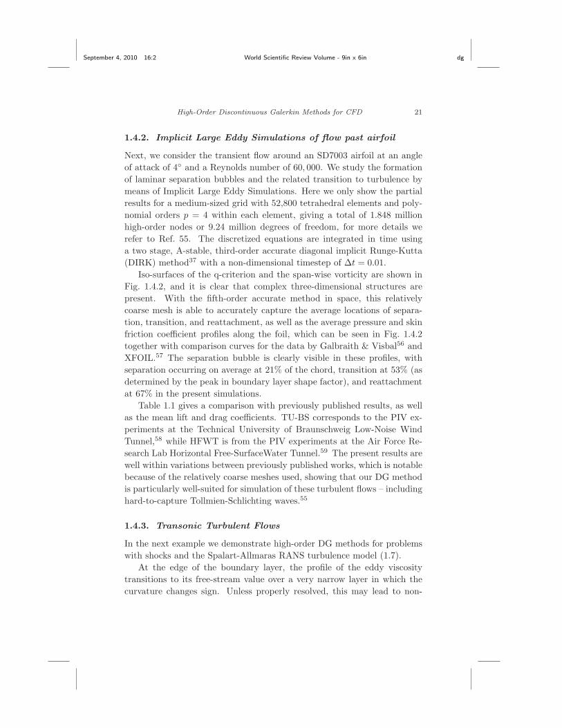
1.4.2. Implicit Large Eddy Simulations of flow past airfoil

Next, we consider the transient flow around an SD7003 airfoil at an angle

of attack of 4 and a Reynolds number of 60, 000. We study the formation

of laminar separation bubbles and the related transition to turbulence by

means of Implicit Large Eddy Simulations. Here we only show the partial

results for a medium-sized grid with 52,800 tetrahedral elements and poly-

nomial orders p = 4 within each element, giving a total of 1.848 million

high-order nodes or 9.24 million degrees of freedom, for more details we

refer to Ref. 55. The discretized equations are integrated in time using

a two stage, A-stable, third-order accurate diagonal implicit Runge-Kutta

(DIRK) method37 with a non-dimensional timestep of ∆t = 0.01.

Iso-surfaces of the q-criterion and the span-wise vorticity are shown in

Fig. 1.4.2, and it is clear that complex three-dimensional structures are

present. With the fifth-order accurate method in space, this relatively

coarse mesh is able to accurately capture the average locations of separa-

tion, transition, and reattachment, as well as the average pressure and skin

friction coefficient profiles along the foil, which can be seen in Fig. 1.4.2

together with comparison curves for the data by Galbraith & Visbal56 and

XFOIL.57 The separation bubble is clearly visible in these profiles, with

separation occurring on average at 21% of the chord, transition at 53% (as

determined by the peak in boundary layer shape factor), and reattachment

at 67% in the present simulations.

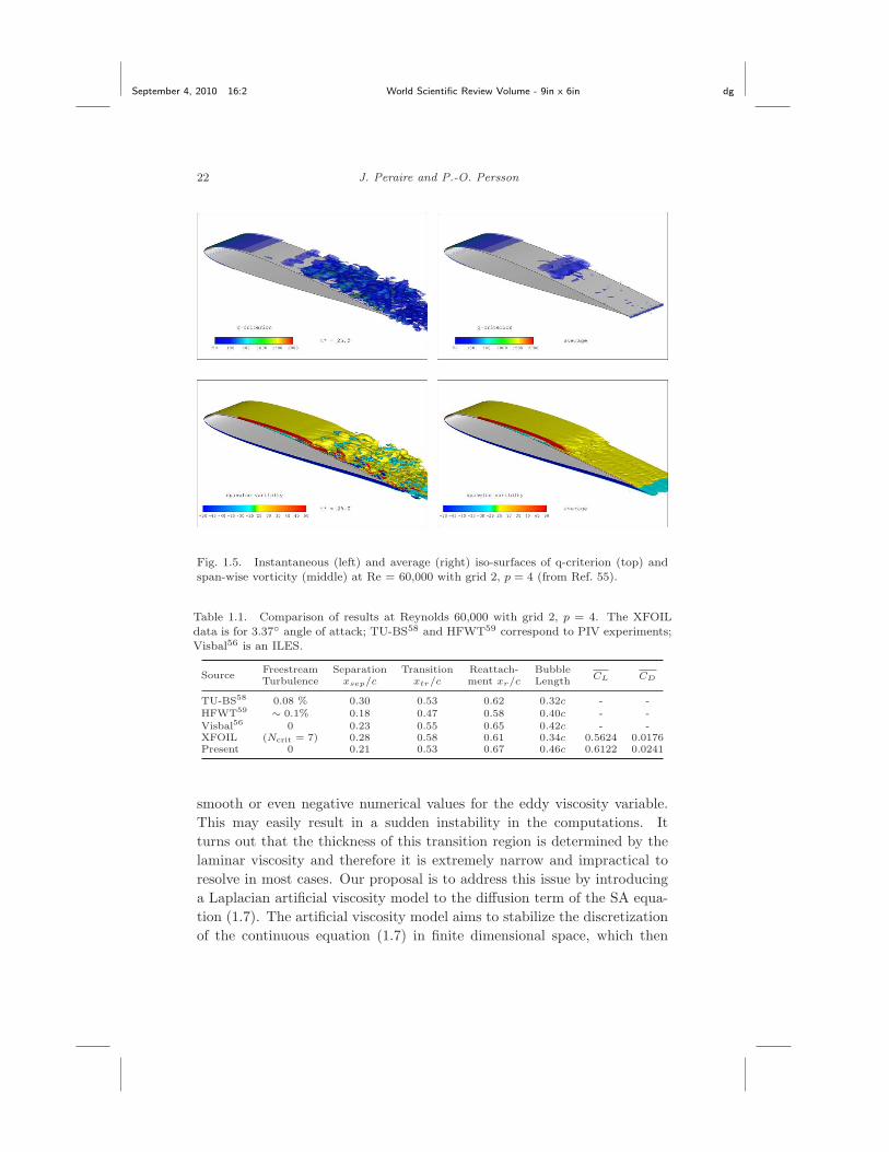
Table 1.1 gives a comparison with previously published results, as well

as the mean lift and drag coefficients. TU-BS corresponds to the PIV ex-

periments at the Technical University of Braunschweig Low-Noise Wind

Tunnel,58 while HFWT is from the PIV experiments at the Air Force Re-

search Lab Horizontal Free-SurfaceWater Tunnel.59 The present results are

well within variations between previously published works, which is notable

because of the relatively coarse meshes used, showing that our DG method

is particularly well-suited for simulation of these turbulent flows – including

hard-to-capture Tollmien-Schlichting waves.55

1.4.3. Transonic Turbulent Flows

In the next example we demonstrate high-order DG methods for problems

with shocks and the Spalart-Allmaras RANS turbulence model (1.7).

At the edge of the boundary layer, the profile of the eddy viscosity

transitions to its free-stream value over a very narrow layer in which the

curvature changes sign. Unless properly resolved, this may lead to non-



Fig. 1.5. Instantaneous (left) and average (right) iso-surfaces of q-criterion (top) andspan-wise vorticity (middle) at Re = 60,000 with grid 2, p = 4 (from Ref. 55).

Table 1.1. Comparison of results at Reynolds 60,000 with grid 2, p = 4. The XFOILdata is for 3.37 angle of attack; TU-BS58 and HFWT59 correspond to PIV experiments;Visbal56 is an ILES.

SourceFreestream Separation Transition Reattach- Bubble

CL CDTurbulence xsep/c xtr/c ment xr/c Length

TU-BS58 0.08 % 0.30 0.53 0.62 0.32c - -HFWT59

∼ 0.1% 0.18 0.47 0.58 0.40c - -Visbal56 0 0.23 0.55 0.65 0.42c - -XFOIL (Ncrit = 7) 0.28 0.58 0.61 0.34c 0.5624 0.0176Present 0 0.21 0.53 0.67 0.46c 0.6122 0.0241

smooth or even negative numerical values for the eddy viscosity variable.

This may easily result in a sudden instability in the computations. It

turns out that the thickness of this transition region is determined by the

laminar viscosity and therefore it is extremely narrow and impractical to

resolve in most cases. Our proposal is to address this issue by introducing

a Laplacian artificial viscosity model to the diffusion term of the SA equa-

tion (1.7). The artificial viscosity model aims to stabilize the discretization

of the continuous equation (1.7) in finite dimensional space, which then



Fig. 1.6. Average pressure coefficient (left) and stream-wise skin friction coefficient(right) at Re = 60,000 on grid 2, p = 4. The dashed lines give XFOIL predictions at3.37, Ncrit = 7. The dot-dashed lines show the ILES data of Galbraith & Visbal.56

accommodates high-order approximations of RANS-SA equations on rela-

tively coarse grids. We point out that the regions where the eddy viscosity

profile is modified have a minor effect on the overall solution since they

generally correspond to regions where the eddy viscosity is very small.

We stabilize our scheme using the artificial viscosity approach in sec-

tion 1.3.2, and add two viscous models of the form:

Fstab(u, q) =

2∑

i=1

h

pε(ψ(si(u)))Fm(u, q) (1.61)

to the regular fluxes. Here, the sensor variables are the eddy viscosity

s1(u) = ν for the turbulence model and the density s2(u) = ρ for the

shocks. As described earlier, the indicator ψ(s) = log10EH/E gives the ra-

tio of high-frequency modes in the sensor s within each element, and the ε

function gives a smooth transition from zero to one. For the viscosity mod-

els F 1(u, q) and F 2(u, q), we use simple Laplacian diffusion added to the

turbulence model and to each of the Navier-Stokes equations, respectively.

Our first validation test is the turbulent flow past a flat plate60 at Rex =

1.02 · 107. We use three grids with 10-by-16 elements (grid C), 19-by-31

elements (grid B), and 37-by-61 elements (grid A), and polynomial degrees

p = 1, . . . , 4 within each element. In addition we solve the problem using a

grid with 72-by-120 elements and p = 4, to be used only for computing a

reference solution for the convergence study.

The velocity profiles and the friction velocities uτ =√

ν∂u/∂y(y = 0)

are shown in Fig. 1.7, together with experimental data. Note how the

high-order p = 4 method on the coarse grid C gives very good agreement



100

101

102

103

104

0

5

10

15

20

25

30

y

u

Law of the wallExp. data

p =4, grid C

p =2, grid B

p =1, grid A

+

+

0 2 4 6 8 10

x 106

0

1

2

3

4

5

6x 10

−3

Rex

Cf

Exp. data

p =4, grid C

p =2, grid B

p =1, grid A

A B C10

−8

10−7

10−6

10−5

10−4

CD

err

or

Grid

p =1

p =2

p =3

p =4

Fig. 1.7. The turbulent flow past a flat plate: (a) velocity profiles at Rex = 1.02× 107,

(b) skin friction coefficient as function of Rex, and (c) errors in drag for the turbulentflow past a flat plate (from Ref. 35).

with both the finer lower-order grids as well as with the experimental data.

Furthermore, the third graph shows grid convergence in the computed drag

forces for all grids at p = 1, . . . , 4. The slopes show good agreement with

the expected dependency O(hp) for differentiated quantities.

We also present results for a turbulent transonic flow past an RAE2822

airfoil at M = 0.729 and Re = 6.5 · 106. We use a single-block, two-

dimensional C-grid with about 1,000 anisotropic triangular elements, and

polynomial degrees p = 4. The grid is clustered around the leading and the

trailing edges and around the airfoil surface to resolve the boundary layer

on the airfoil, as well as around the shock. The first grid point off the wall

is at a distance of 5× 10−5 from the airfoil surface.

The resulting flow field is shown in Fig. 1.4.3. We note how the high-

order stretched elements resolve the boundary layer even if the elements

are large, and that the artificial viscosity approach resolves the shock with

subgrid accuracy.

1.4.4. Flapping Elliptic Wings

Our final example is the transient laminar flow around a pair of flapping

wings.61 We consider a wing pair with an elliptical planform. The max-

imum normalized chord at the wing centerline is c = 1 and the wing tip-

to-tip span is b = 10. The flapping motions occur symmetrically about a

hinge located at the wing centerline. An HT13 airfoil is selected for the

entire wing span, resulting in a maximum wing thickness of t = 0.065 at

the wing centerline.

In order to obtain maximum geometrical flexibility, the equations are

discretized on unstructured meshes of triangles and tetrahedra. We use the

symmetry of the problem to only simulate one half of the domain, with



Fig. 1.8. Transonic flow (M = 0.729,Re = 6.5 · 106), with subcell resolution of shocks.

a symmetry boundary condition at the cut plane. We generate all the

surface meshes in parametrized form using the DistMesh triangular mesh

generator.62 The tetrahedral volume mesh is then generated by a Delaunay

refinement based code.63 The resulting mesh has about 43,000 nodes and

231,000 tetrahedral elements for the half-domain, which corresponds to

4.62 million high-order nodes with polynomial orders of degree p = 3. To

account for the curved domain boundaries, we use the nonlinear elasticity

approach that we proposed in Ref. 64. The mesh is shown in Fig. 1.9.

We prescribe the symmetric wing motion using a flapping angle at the

wing centerline hinge given by

φ(t) = Aφ cosωt (1.62)

where t is the time, Aφ = 30 is the flapping amplitude and w = 2π/20 the

flapping angular frequency. In addition, a wing twist angle is prescribed as

a function of the span location. At the distance X from the centerline of

the wing, the twist angle is

θ(t,X) = ε (a(X) cosωt+ b(X) cosωt)



Fig. 1.9. A tetrahedral mesh for the domain around the elliptic wing pair.

where the twist scaling factor ε ∈ [0, 1] is a parameter that controls the

amount of spanwise twist, and the coefficients a(X), b(X) are chosen to

locally align the wing with the flow:61

A(X) = −√L2 −X2

4u∞L, B(X) =

Xφ0ω

u∞, (1.63)

a(X) =−B

A2ω2 + 1, b(X) =

BAω

A2ω2 + 1. (1.64)

We note that this motion is not in any way an optimized flapping strategy,

but it is adequate for the purposes of studying our computational models.

In order to develop an ALE formulation for this domain deformation,

we need a smooth embedding of the flapping motion φ(t), θ(t,X) in the

reference domain. That is, we need a smooth function x = x(t,X) that

maps the wing surface to the location given by φ(t), θ(t,X). We also prefer

volume preserving mappings (g = 1) to simplify the ALE equations.

While there are many ways to find such a mapping, we use a shearing

approach as follows. To begin with, the function A(X) is not differentiable

at X = L, and not even real-valued for X > L, so we need to modify the

flapping motion to regularize this expression. We approximate

√

L2 −X2 ≈ arctan(r(L−X))

arctan(rL)L (1.65)

where r = 1.2 is a good choice. Note that this expression is also defined

and smooth for X > L. The mapping functions are then created using two

combined shearing motions, which gives a volume-preserving deformation



gradient (det(G) = 1):

x(X, t) =

X cosφ

Y cos θ

X sinφ+ Y sin θ

+Z secφ sec θ

, G =

cosφ 0 0

G21 cos θ 0

G31 G32 secφ sec θ

, (1.66)

where all matrix entries as well as the grid velocity ∂x/∂t are found by

analytical differentiation.

Our simulations are done at a Reynolds number of Re = 3, 000 and a

free-stream Mach number ofM = 0.1. We use a third-order accurate diago-

nal implicit Runge-Kutta (DIRK) method37 for time-integration, and poly-

nomials of degree p = 3 within each tetrahedron for the space discretization.

This gives a total of about 23 million degrees of freedom, and we integrate

for three full flapping cycles using 600 implicit timesteps. We solve on a

parallel computer with 32 nodes and a total of 256 computing processes,

using the parallel Newton-Krylov methods described in section 1.3.3.

We show two representative test cases with different free-stream angle

of attack α and twist scaling factor ε. Visualizations of these flow fields

are shown in Fig. 1.10, where the Mach number is plotted as color on

isosurfaces of the entropy. The flow plots show regions of flow separation

and wake vortex structures. For the first case (α = 5, ε = 0.5), significant

separation occurs over the entire wing during the mid-to-late downstroke.

In the second case (α = 10, ε = 1.0), there is separation throughout the

entire flapping cycle, in particular inboard of the wing.

The time evolution of the vertical and horizontal forces are shown in

Fig. 1.11, along with a comparison with a simpler panel method code65

based on a potential flow model. We note that the panel method code

predicts the lift forces well in the first case, although it over-predicts the

thrust production somewhat. In the second case, due to the large amount

of separation during the downstroke, the force predictions do not agree well.

Therefore, we can conclude that low-fidelity simulation tools can perform

well for attached flows, but high-fidelity Navier-Stokes solvers are essential

for predicting flows with large amounts of separation.

1.5. Acknowledgements

We would like to acknowledge our collaborators J. Bonet, M. Drela, E. Is-

raeli, C. N. Nguyen, A. Uranga, and D. J. Willis for the many contributions

to the work reported in this chapter.



Angle of attack α = 5, twist multiplier ε = 0.5

Angle of attack α = 10, twist multiplier ε = 1.0

Fig. 1.10. The flow field around the flapping wing pair, visualized as Mach numbercolor plots on isosurfaces of the entropy. The plots correspond to two representativecases of angle of attack and twist multiplier (top and bottom) and the times t = 20,

t = 25, and t = 30 (left to right).

0 10 20 30 40 50 60−2

−1.5

−1

−0.5

0

0.5Drag Force ( AoA α = 5o, ε = 0.5 )

0 10 20 30 40 50 60−2

0

2

4

6Lift Force ( AoA α = 5o, ε = 0.5 )

0 10 20 30 40 50 60

−1

−0.5

0

0.5

1

Drag Force ( AoA α = 10o, ε = 1.0 )

0 10 20 30 40 50 600

1

2

3

4Lift Force ( AoA α = 10o, ε = 1.0 )

High−Order DG (Navier−Stokes)Panel Method (Potential flow)

Fig. 1.11. The lift coefficients computed by the two simulation codes for the two casesconsidered (α = 5, ε = 0.5 and α = 10, ε = 1.0).



References

1. S. K. Lele, Compact finite difference schemes with spectral-like resolution, J.Comput. Phys. 103(1), 16–42, (1992).

2. M. R. Visbal and D. V. Gaitonde, On the use of higher-order finite-differenceschemes on curvilinear and deforming meshes, J. Comput. Phys. 181(1),155–185, (2002).

3. T. J. Barth. Recent developments in high-order k-exact reconstruction onunstructured meshes, (1993). AIAA-93-0668.

4. A. Nejat and C. Ollivier-Gooch, A high-order accurate unstructured finitevolume Newton-Krylov algorithm for inviscid compressible flows, J. Comput.Phys. 227(4), 2582–2609, (2008).

5. T. Hughes, G. Scovazzi, and T. Tezduyar, Stabilized methods for compress-ible flows, SIAM J. Sci. Comput. 43, 343–368, (2010).

6. W. H. Reed and T. R. Hill. Triangular mesh methods for the neutrontransport equation. Technical Report Technical Report LA-UR-73-479, LosAlamos Scientific Laboratory, (1973).

7. B. Cockburn and C.-W. Shu, Runge-Kutta discontinuous Galerkin methodsfor convection-dominated problems, J. Sci. Comput. 16(3), 173–261, (2001).

8. J. S. Hesthaven and T. Warburton, Nodal discontinuous Galerkin methods.vol. 54, Texts in Applied Mathematics, (Springer, New York, 2008). Algo-rithms, analysis, and applications.

9. B. Cockburn, J. Gopalakrishnan, and R. Lazarov, Unified hybridization ofdiscontinuous Galerkin, mixed, and continuous Galerkin methods for secondorder elliptic problems, SIAM J. Numer. Anal. 47(2), 1319–1365, (2009).

10. N. C. Nguyen, J. Peraire, and B. Cockburn, An implicit high-order hybridiz-able discontinuous galerkin method for the incompressible navier-stokes equa-tions, J. Comput. Phys. (2010). To appear.

11. J. Peraire, N. C. Nguyen, and B. Cockburn. A hybridizable discontinu-ous galerkin method for the compressible euler and navier-stokes equations.In 48th AIAA Aerospace Sciences Conference, Orlando, Florida (January,2010). AIAA-2010-363.

12. Z. J. Wang, Spectral (finite) volume method for conservation laws on unstruc-tured grids. Basic formulation, J. Comput. Phys. 178(1), 210–251, (2002).

13. Y. Liu, M. Vinokur, and Z. J. Wang, Spectral difference method for un-structured grids. I. Basic formulation, J. Comput. Phys. 216(2), 780–801,(2006).

14. J. P. Boris, On Large Eddy Simulation using subgrid turbulence models.(Springer-Verlag, New York, 1990). In J.L. Lumley, editor, Whither Tur-bulence? Turbulence at the Crossroads.

15. P. R. Spalart and S. R. Allmaras, A one-equation turbulence model for aero-dynamic flows, La Rech. Aerospatiale. 1, 5–21, (1994).

16. P.-O. Persson, J. Bonet, and J. Peraire, Discontinuous Galerkin solution ofthe Navier-Stokes equations on deformable domains, Comput. Methods Appl.Mech. Engrg. 198(17-20), 1585–1595, (2009).

17. P. D. Thomas and C. K. Lombard, Geometric conservation law and its ap-



plication to flow computations on moving grids, AIAA J. 17(10), 1030–1037,(1979).

18. P. L. Roe, Approximate Riemann solvers, parameter vectors, and differenceschemes, J. Comput. Phys. 43(2), 357–372, (1981).

19. J. Peraire and P.-O. Persson, The compact discontinuous Galerkin (CDG)method for elliptic problems, SIAM J. Sci. Comput. 30(4), 1806–1824,(2008).

20. B. Cockburn and C.-W. Shu, The local discontinuous Galerkin method fortime-dependent convection-diffusion systems, SIAM J. Numer. Anal. 35(6),2440–2463, (1998).

21. B. Cockburn and B. Dong. An analysis of the minimal dissipation lo-cal discontinuous Galerkin method for convection–difussion problems. IMAPreprint Series # 2146, also presented at the 7th. World Congress on Com-putational Mechanics, Los Angeles, CA, June 16-22, 2006, (2006).

22. C. E. Baumann and J. T. Oden, A discontinuous hp finite element methodfor the Euler and Navier-Stokes equations, Int. J. Numer. Methods Fluids.31(1), 79–95, (1999). Tenth International Conference on Finite Elements inFluids (Tucson, AZ, 1998).

23. A. Burbeau, P. Sagaut, and C.-H. Bruneau, A problem-independent lim-iter for high-order Runge-Kutta discontinuous Galerkin methods, J. Comput.Phys. 169(1), 111–150, (2001).

24. C.-W. Shu and S. Osher, Efficient implementation of essentially nonoscilla-tory shock-capturing schemes, J. Comput. Phys. 77(2), 439–471, (1988).

25. C.-W. Shu and S. Osher, Efficient implementation of essentially nonoscilla-tory shock-capturing schemes. II, J. Comput. Phys. 83(1), 32–78, (1989).

26. I. Lomtev, C. B. Quillen, and G. E. Karniadakis, Spectral/hp methods forviscous compressible flows on unstructured 2D meshes, J. Comput. Phys.144(2), 325–357, (1998).

27. A. Kanevsky, M. H. Carpenter, and J. S. Hesthaven, Idempotent filteringin spectral and spectral element methods, J. Comput. Phys. 220(1), 41–58,(2006).

28. E. Tadmor, Shock capturing by the spectral viscosity method, Comput. Meth-ods Appl. Mech. Engrg. 80(1-3), 197–208, (1990). Spectral and high ordermethods for partial differential equations (Como, 1989).

29. S. Hesthaven, J.S. Kaber and L. Lurati, Pade-legendre interpolants for gibbsreconstruction, J. Sci. Comput. (2005). (to appear).

30. G. May and A. Jameson. High-order accurate methods for high-speed flow.In 17th AIAA Computational Fluid Dynamics Conference, Toronto, Ontario(June, 2005). AIAA-2005-5252.

31. P.-O. Persson and J. Peraire. Sub-cell shock capturing for discontinuousGalerkin methods. In 44th AIAA Aerospace Sciences Meeting and Exhibit,Reno, Nevada, (2006). AIAA-2006-0112.

32. J. Von Neumann and R. D. Richtmyer, A method for the numerical calcula-tion of hydrodynamic shocks, J. Appl. Phys. 21, 232–237, (1950).

33. G. E. Barter. Shock capturing with PDE-based artificial viscosity for an adap-tive, higher-order discontinuous Galerkin finite element method. PhD thesis,



M.I.T. (June, 2008).34. F. Bassi, A. Crivellini, S. Rebay, and M. Savini, Discontinuous Galerkin

solution of the Reynolds-averaged Navier-Stokes and k−ω turbulence modelequations, Computers & Fluids. 34(4–5), 507–540, (2005).

35. N. C. Nguyen, P.-O. Persson, and J. Peraire. RANS solutions using high orderdiscontinuous Galerkin methods. In 45th AIAA Aerospace Sciences Meetingand Exhibit, Reno, Nevada, (2007). AIAA-2007-914.

36. T. H. Koornwinder. Askey-Wilson polynomials for root systems of type BC.In Hypergeometric functions on domains of positivity, Jack polynomials, andapplications (Tampa, FL, 1991), vol. 138, Contemp. Math., pp. 189–204.Amer. Math. Soc., Providence, RI, (1992).

37. R. Alexander, Diagonally implicit Runge-Kutta methods for stiff o.d.e.’s,SIAM J. Numer. Anal. 14(6), 1006–1021, (1977).

38. L. F. Shampine and C. W. Gear, A user’s view of solving stiff ordinarydifferential equations, SIAM Rev. 21(1), 1–17, (1979).

39. E. Anderson et al., LAPACK Users’ Guide. (Society for Industrial and Ap-plied Mathematics, Philadelphia, PA, 1999), third edition.

40. P.-O. Persson and J. Peraire, Newton-GMRES preconditioning for discontin-uous Galerkin discretizations of the Navier-Stokes equations, SIAM J. Sci.Comput. 30(6), 2709–2733, (2008).

41. P.-O. Persson. Scalable parallel Newton-Krylov solvers for discontinuousGalerkin discretizations. In 47th AIAA Aerospace Sciences Meeting and Ex-hibit, Orlando, Florida, (2009). AIAA-2009-606.

42. C. R. Nastase and D. J. Mavriplis, High-order discontinuous Galerkin meth-ods using an hp-multigrid approach, J. Comput. Phys. 213(1), 330–357,(2006).

43. K. Fidkowski, T. Oliver, J. Lu, and D. Darmofal, p-multigrid solution ofhigh-order discontinuous Galerkin discretizations of the compressible Navier-Stokes equations, J. Comput. Phys. 207(1), 92–113, (2005).

44. G. Kanschat, Robust smoothers for high-order discontinuous galerkin dis-cretizations of advection-diffusion problems, J. Comput. Appl. Math. 218

(1), 53–60, (2008).45. L. T. Diosady and D. L. Darmofal, Preconditioning methods for discontinu-

ous Galerkin solutions of the Navier-Stokes equations, J. Comput. Phys. 228(11), 3917–3935, (2009).

46. W. Hackbusch, Multigrid methods and applications. vol. 4, Springer Seriesin Computational Mathematics, (Springer-Verlag, Berlin, 1985).

47. E. M. Rønquist and A. T. Patera, Spectral element multigrid. I. Formulationand numerical results, J. Sci. Comput. 2(4), 389–406, (1987).

48. P. Wesseling. A robust and efficient multigrid method. In Multigrid methods(Cologne, 1981), vol. 960, Lecture Notes in Math., pp. 614–630. Springer,Berlin, (1982).

49. G. Wittum. On the robustness of ILU-smoothing. In Robust multi-grid meth-ods (Kiel, 1988), vol. 23, Notes Numer. Fluid Mech., pp. 217–239. Vieweg,Braunschweig, (1989).

50. H. C. Elman, V. E. Howle, J. N. Shadid, and R. S. Tuminaro, A parallel block



multi-level preconditioner for the 3D incompressible Navier-Stokes equations,J. Comput. Phys. 187(2), 504–523, (2003).

51. W. L. Briggs, V. E. Henson, and S. F. McCormick, A multigrid tutorial.(Society for Industrial and Applied Mathematics (SIAM), Philadelphia, PA,2000), second edition.

52. A. Toselli and O. Widlund, Domain Decomposition Methods - Algorithms andTheory. vol. 34, Springer Series in Computational Mathematics, (Springer,2004).

53. G. Karypis and V. Kumar. METIS serial graph partitioning and fill-reducingmatrix ordering. http://glaros.dtc.umn.edu/gkhome/metis/metis/overview.

54. C.-D. Munz, S. Roller, R. Klein, and K. J. Geratz, The extension of incom-pressible flow solvers to the weakly compressible regime, Comput. & Fluids.32(2), 173–196, (2003).

55. A. Uranga, P.-O. Persson, M. Drela, and J. Peraire, Implicit large eddysimulation of transition to turbulence at low Reynolds numbers using a dis-continuous Galerkin method, Int. J. Num. Meth. Eng. (2010). To appear.

56. M. Galbraith and M. Visbal. Implicit Large Eddy Simulaion of low Reynoldsnumber flow past the SD7003 airfoil. In Proc. of the 46th AIAA AerospaceSciences Meeting and Exhibit, Reno, Nevada, AIAA-2008-225, (2008).

57. M. Drela. XFOIL Users Guide, Version 6.94. MIT Aeronautics and Astro-nautics Department, (2002).

58. R. Radespiel, J. Windte, and U. Scholz, Numerical and experimental flowanalysis of moving airfoils with laminar separation bubbles, AIAA Paper2006-501. (Jan. 2006.).

59. M. Ol, B. McAuliffe, E. Hanff, U. Scholz, and C. Kahler. Comparison of lam-inar separation bubbles measurements on a low Reynolds number airfoil inthree facilities. In Proc. of the 35th Fluid Dynamics Conference and Exhibit,Toronto, Ontario, Canada, AIAA-2005-5149, (2005).

60. D. Coles and E. Hirst. Computation of turbulent boundary layers. In AFOSR-IFP-Stanford Conference, vol. II, CA, (1969). Stanford University.

61. P.-O. Persson, D. J. Willis, and J. Peraire. The numerical simulation of flap-ping wings at low reynolds numbers. In 48th AIAA Aerospace Sciences Meet-ing and Exhibit, Orlando, Florida, (2010). AIAA-2010-724.

62. P.-O. Persson and G. Strang, A simple mesh generator in Matlab, SIAM Rev.46(2), 329–345, (2004).

63. K. Morgan and J. Peraire, Unstructured grid finite element methods for fluidmechanics, Inst. of Physics Reviews. 61(6), 569–638, (1998).

64. P.-O. Persson and J. Peraire. Curved mesh generation and mesh refinementusing Lagrangian solid mechanics. In 47th AIAA Aerospace Sciences Meetingand Exhibit, Orlando, Florida, (2009). AIAA-2009-949.

65. D. J. Willis, J. Peraire, and J. K. White, A combined pFFT-multipole treecode, unsteady panel method with vortex particle wakes, Internat. J. Numer.Methods Fluids. 53(8), 1399–1422, (2007).

Chapter 1 High-Order Discontinuous Galerkin...

Documents

Transcript of Chapter 1 High-Order Discontinuous Galerkin...