CHAPTER 1 - GEOPHYSICAL PERSPECTIVE - UMass D · CHAPTER 1 - GEOPHYSICAL ... Figure 1.3 (right) A...

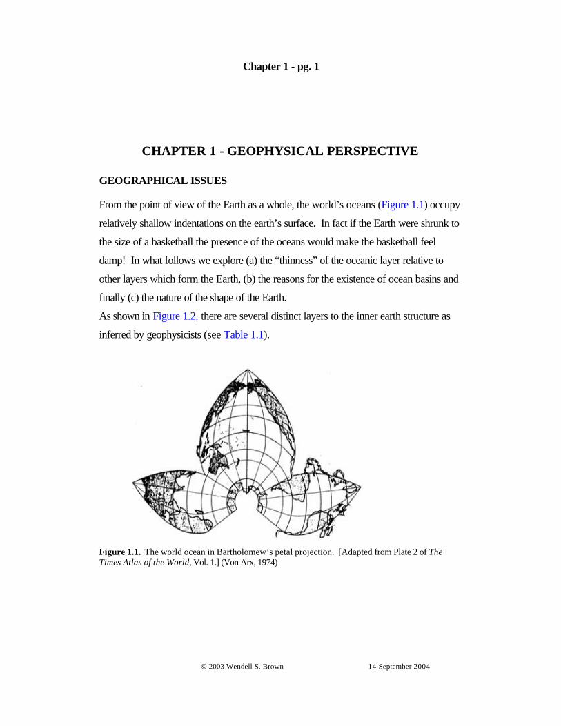
Chapter 1 - pg. 1

© 2003 Wendell S. Brown 14 September 2004

CHAPTER 1 - GEOPHYSICAL PERSPECTIVE GEOGRAPHICAL ISSUES From the point of view of the Earth as a whole, the world’s oceans (Figure 1.1) occupy

relatively shallow indentations on the earth’s surface. In fact if the Earth were shrunk to

the size of a basketball the presence of the oceans would make the basketball feel

damp! In what follows we explore (a) the “thinness” of the oceanic layer relative to

other layers which form the Earth, (b) the reasons for the existence of ocean basins and

finally (c) the nature of the shape of the Earth.

As shown in Figure 1.2, there are several distinct layers to the inner earth structure as

inferred by geophysicists (see Table 1.1).

Figure 1.1. The world ocean in Bartholomew’s petal projection. [Adapted from Plate 2 of The Times Atlas of the World, Vol. 1.] (Von Arx, 1974)

Chapter 1 - pg. 2


Figure 1.2. Layers of the earth. The core, about 7,000 km. (4,400 miles) in diameter, consists of exceedingly hot, dense material. It is thought to have two parts: a solid center and a liquid outer layer. Surrounding the core is the mantle, about 2,000 km. (1,800 miles) of dense rock. Next is the crust, or outermost layer of the earth. This is very thin in comparison, its thickness varying from as little as 5 km. (3 miles) to at most 50 km. (30 miles). (Ericson & Wollin, 1967).

The most striking feature of Table 1.1 is the increase of density with depth. This

understanding along with other geophysical data including the relatively small gravity

anomalies observed over the Earth’s surface has led scientists to conclude that these

layers of the Earth are in isostatic equilibrium. The situation of isostasy is consistent

with the fact that on average layers within the Earth “float on one another”. (The special

case of this situation in water is hydrostatic equilibrium).

Isostasy and the large difference in thickness between continental and oceanic crust

explains the existence of ocean “basins”. Archimedes principle tells us two things; (1) a

piece of buoyant (i.e. floating) material, such as wood in water, that is less dense than an

equally thick piece of more dense material will rise higher in a fluid and (2) a piece of

buoyant material that is thicker than a thinner piece of equally dense material will also

rise higher in a fluid. As shown in Figure 1.3, the thicker continental crust “floats”

Chapter 1 - pg. 3


higher in the mantle below relative to the thinner oceanic crust. The density differences

of the earth crustal layers are so small that they are much less important than layer

thickness differences. (The Theory of Seafloor Spreading and Plate Tectonics explains

why the densities and thicknesses of the different crustal layers differ).

To understand the physics of this and other Earth configurations, we need to know a

little bit about how the Earth responds to different forces. When sustained loads are

applied over geologic time scales, Earth material flows like a fluid and undergoes

permanent deformation sometimes known as “plastic deformation.” The same kind

of behavior is observed when loads, which have been applied for long periods of

geologic time, are “suddenly” released. For example, Scandinavia is still rising at the

rate of about 1 cm per year in response to the melting of the last glacier 10,000 years

ago.

When loading is applied to the Earth on time scales that are short compared to

geological time scales, the Earth exhibits “elastic deformation” – that is it distorts and

springs back to its original configuration. For example, the Earth’s surface temporarily

bulges outward about 1 meter in response to moon- and sun-induced tidal forcing.

How are these ideas relevant to the Earth’s surface configuration in general and the

Figure 1.3 (right) A hypothetical section of the earth’s crustal layer – as defined at depth by the “Moho” discontinuity. Note that the continental crust in the mountain region plunges much further into the mantle than does the relativey thin oceanic crust to the left. (left) This earth geological configuration can be modeled with slabs of wood floating in a fluid.

Chapter 1 - pg. 4


oceans in particular? First we know that the earth is almost a sphere. In fact, the 3rd

century B.C. Greek astronomer Eratosthenes assumed a spherical Earth and estimated

its circumference reasonably accurately. (I wonder if the sailors between his and

Columbus time knew of this computation).

The Earth, however, is actually an ellipsoid with a polar radius which is 22 km less than

the equatorial radius. To understand why, consider a rotating spherical earth (Figure

1.4). Here each “parcel” of earth material is acted upon by centrifugal force (per unit

mass) of cr

, a vector that can be resolved into its locally vertical vcr

and horizontal hcr

components (see the Appendix ). The vertical component vcr

can not move an earth

parcel upward (hence no distortion) because it is opposed by the very large

gravitational force per unit mass (i.e. .1|g

| v pprrc ). On the other hand, hc

ris unopposed -

a non-equilibrium situation in which Earth material will be forced to move horizontally

equatorward until a non-spherical, dynamic equilibrium Earth configuration arises.

g

c cv

ch

Figure 1.4. Centrifugal force due to earth rotation results in an unbalanced horizontal force component ch on a spherical earth.

Chapter 1 - pg. 5


As a consequence of this tendency for deformation toward a dynamic equilibrium

configuration, the Earth has had an ellipsoidal shape throughout its approximate 13

billion year history (see Figure 1.5). The actual dimensions of the ellipsoidal shape have

changed with time because the Earth rotation rate has been slowly decreasing since its

formation (due to ocean tidal friction).

Why an ellipsoidal shape? It turns out that the dynamic equilibrium configuration of a

rotating Earth is one with an elliptical cross-section. The surface Earth material does not

move in this equilibrium configuration. This occurs because the component of geocentric

gravitational force (per unit mass) that is tangent to the Earth’s surface gr

h is equal and

opposite to the tangential component of the “centrifugal force” (per unit mass) .cr

h

Note that the “effective gravitational force” g′r (i.e. locally perpendicular to the Earth

surface) is the vector sum of the geocentric gravitational force ,g ,r

and the centrifugal

force .cr

Because the centrifugal force is so much smaller than the gravitational force, the

geometrical angle a between ,g ,r

and g′r is very small. (Later you will have a chance to

show that the angle is less than a degree). Due to an increased centrifugal force at

Figure 1.5. Force balances for an rotating ellipsoidal Earth in dynamic equilibrium. Note that the local tangential components of the geocentric gravitational force (per unit mass) gh and centrifugal force ch are equal.

Chapter 1 - pg. 6


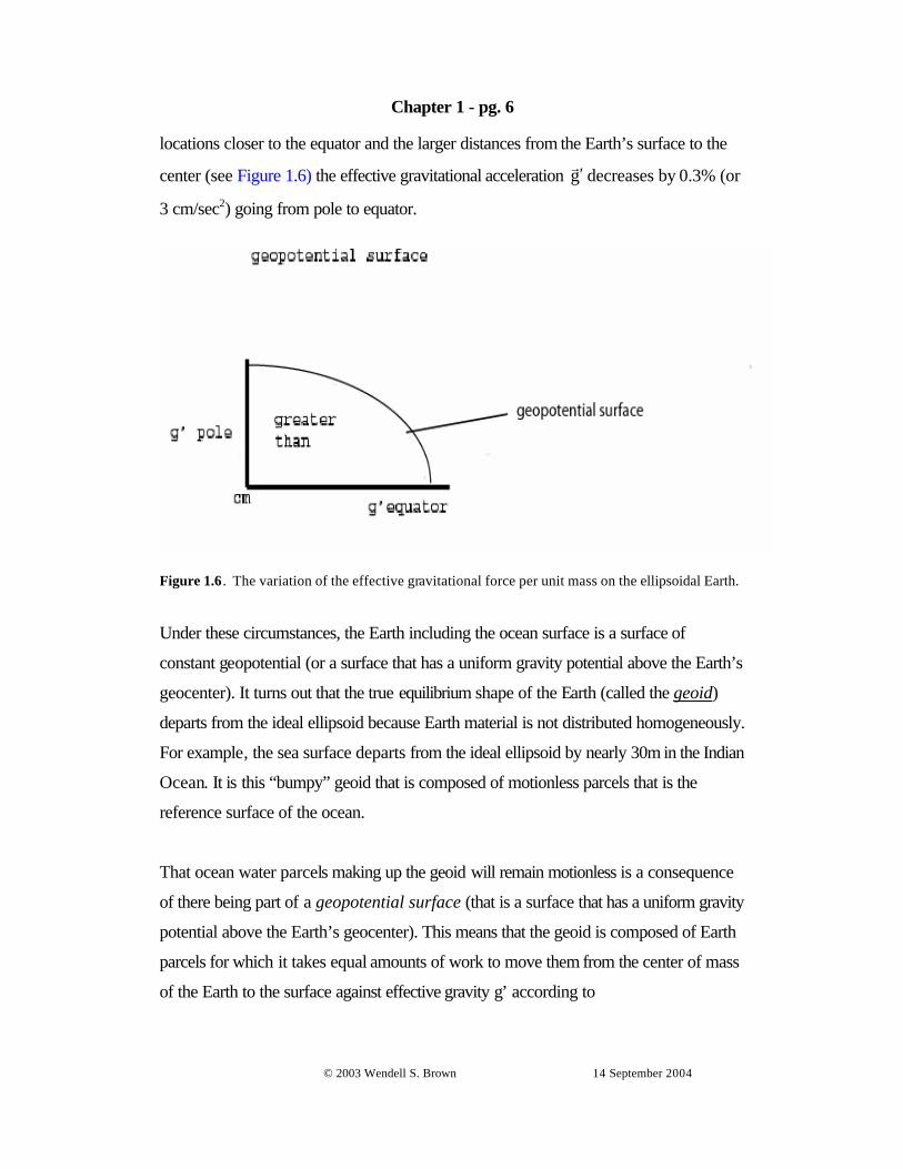
locations closer to the equator and the larger distances from the Earth’s surface to the

center (see Figure 1.6) the effective gravitational acceleration g′r decreases by 0.3% (or

3 cm/sec2) going from pole to equator.

Figure 1.6 . The variation of the effective gravitational force per unit mass on the ellipsoidal Earth.

Under these circumstances, the Earth including the ocean surface is a surface of

constant geopotential (or a surface that has a uniform gravity potential above the Earth’s

geocenter). It turns out that the true equilibrium shape of the Earth (called the geoid)

departs from the ideal ellipsoid because Earth material is not distributed homogeneously.

For example, the sea surface departs from the ideal ellipsoid by nearly 30m in the Indian

Ocean. It is this “bumpy” geoid that is composed of motionless parcels that is the

reference surface of the ocean.

That ocean water parcels making up the geoid will remain motionless is a consequence

of there being part of a geopotential surface (that is a surface that has a uniform gravity

potential above the Earth’s geocenter). This means that the geoid is composed of Earth

parcels for which it takes equal amounts of work to move them from the center of mass

of the Earth to the surface against effective gravity g’ according to

Chapter 1 - pg. 7


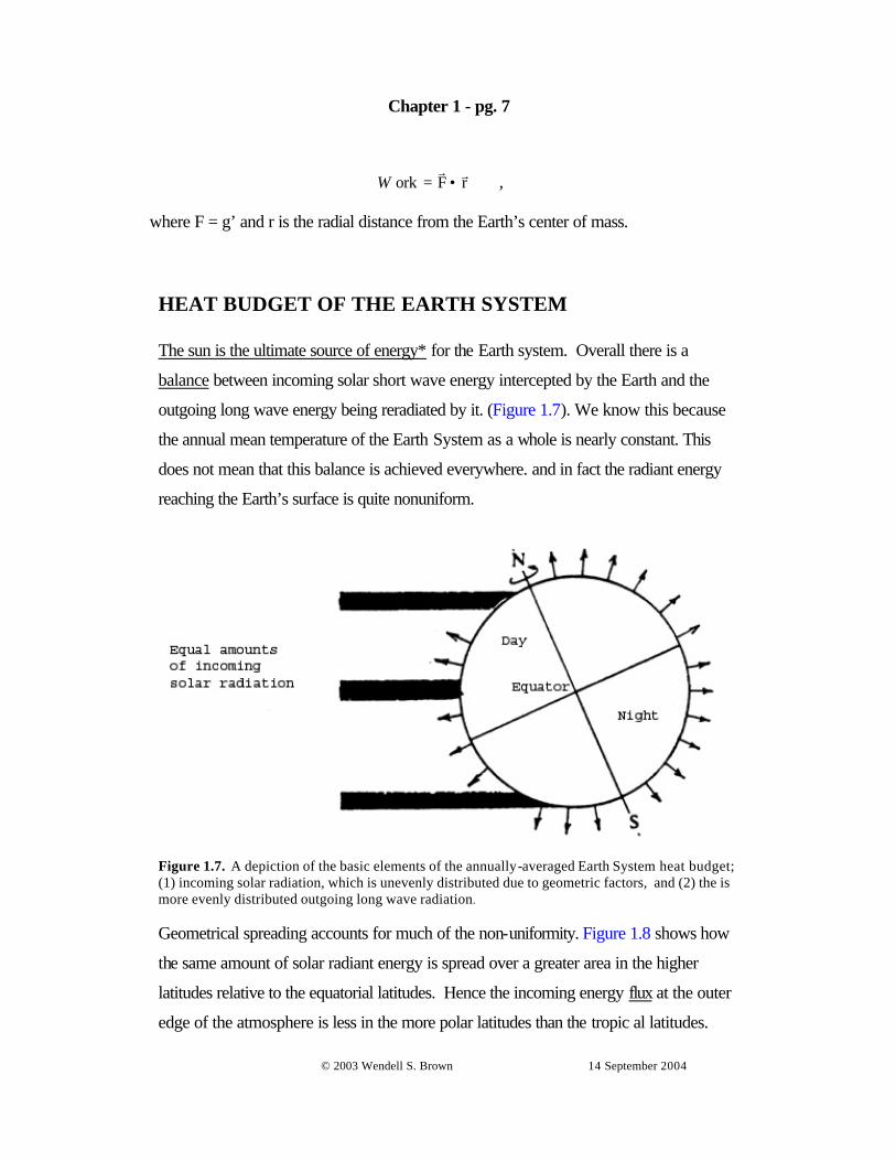
HEAT BUDGET OF THE EARTH SYSTEM The sun is the ultimate source of energy* for the Earth system. Overall there is a

balance between incoming solar short wave energy intercepted by the Earth and the

outgoing long wave energy being reradiated by it. (Figure 1.7). We know this because

the annual mean temperature of the Earth System as a whole is nearly constant. This

does not mean that this balance is achieved everywhere. and in fact the radiant energy

reaching the Earth’s surface is quite nonuniform.

Figure 1.7. A depiction of the basic elements of the annually-averaged Earth System heat budget; (1) incoming solar radiation, which is unevenly distributed due to geometric factors, and (2) the is more evenly distributed outgoing long wave radiation. Geometrical spreading accounts for much of the non-uniformity. Figure 1.8 shows how

the same amount of solar radiant energy is spread over a greater area in the higher

latitudes relative to the equatorial latitudes. Hence the incoming energy flux at the outer

edge of the atmosphere is less in the more polar latitudes than the tropic al latitudes.

r F =ork rr

•W , where F = g’ and r is the radial distance from the Earth’s center of mass.

Chapter 1 - pg. 8


However the distribution of outgoing long wave energy is much more even over the

earth at the edge of the atmosphere than is that of solar radiation energy. Consequently

there is a surplus of incoming solar energy at the edge of the atmosphere in the

equatorial regions and deficit of incoming solar energy to supply the long wave radiation

demand.

The amount of heat flux reaching different areas of the Earth will also be affected by the

local length of day. The actual amount of heat flux which eventually reaches the Earth’s

surface will be affected by other factors, including the amount of (1) absorption by

dust; (2) cloud absorption and scatter and (3) surface reflection due to ice cover, etc.

The overall heat budget of the Earth at the surface varies with latitude in a way shown in

Figure 1.9. The thermal energy imbalances implied by in Figure 1.9 are the basis for the

poleward heat transport by the atmosphere/ocean system (Figure 1.10). The combined

ocean and atmospheric circulation (weather) result from this thermal energy gradient.

Figure 1.8. Equal amounts of solar energy at (a) are spread over increasingly larger areas at more polar latitudes as illustrated in (b) and (c) respectively. (Duxbury & Duxbury, 1984)

Chapter 1 - pg. 9


Most of the direct solar energy is absorbed initially by the land and oceans. Because of

the ocean’s extensiveness (71% of the Earth surface) and relatively high heat capacity, it

is the principal heat reservoir in the Earth system. The atmosphere with its relatively low

heat capacity is principally a conveyor of heat from the equatorial regions to the polar

regions. The exchange of heat between the ocean and atmosphere is affected by a

complex suite of heat transfer processes. Heat from the ocean causes atmospheric

winds, which in turn cause ocean currents. The winds and the oceans partner to move

heat poleward.

.

Figure 1.9. (a) Incoming (solar insulation) and outgoing heat flux as a function of latitude, (b) Ocean surface temperature distributions.

Chapter 1 - pg. 10


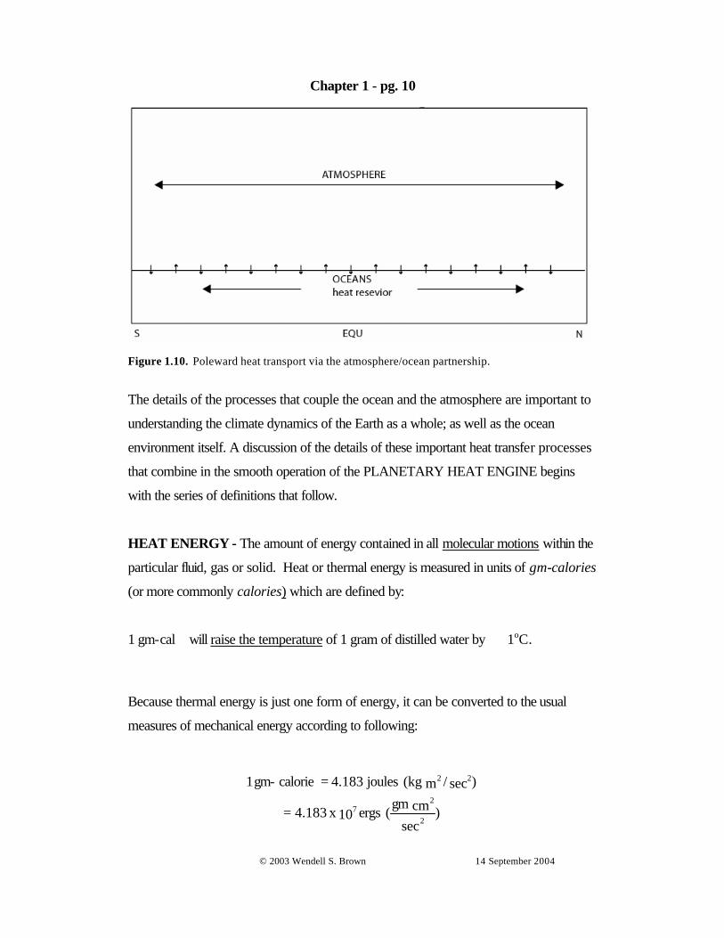
Figure 1.10. Poleward heat transport via the atmosphere/ocean partnership.

The details of the processes that couple the ocean and the atmosphere are important to

understanding the climate dynamics of the Earth as a whole; as well as the ocean

environment itself. A discussion of the details of these important heat transfer processes

that combine in the smooth operation of the PLANETARY HEAT ENGINE begins

with the series of definitions that follow.

HEAT ENERGY - The amount of energy contained in all molecular motions within the

particular fluid, gas or solid. Heat or thermal energy is measured in units of gm-calories

(or more commonly calories) which are defined by:

1 gm-cal will raise the temperature of 1 gram of distilled water by 1oC.

Because thermal energy is just one form of energy, it can be converted to the usual

measures of mechanical energy according to following:

)

seccm gm

( ergs 10 x 4.183 =

)sec/m (kg joules 4.183 = caloriegm- 1

2

27

22

Chapter 1 - pg. 11


This means that the frictional process of stirring 4.183 x 107 ergs of mechanical energy

into 1 gm of water will raise it’s temperature by 1oC.

SPECIFIC HEAT or HEAT CAPACITY (Cp) - The amount of heat energy required

to raise 1 gm of material by 1oC, when working at constant pressure.

The specific heat of water, which depends weakly on salinity (S), temperature (T) and

pressure (p), is relatively high in comparison to other common Earth materials , for

which .Ccal/gm/ .2 0 Cp °≅

HEAT FLUX (Q) - The amount of heat energy passing through a unit area in a unit

time. Heat flux is measured in units of cal/cm2/sec (or langleys / sec or ly/sec).

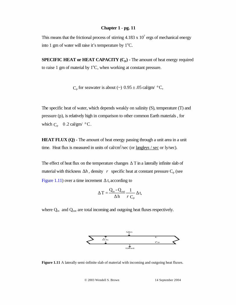
The effect of heat flux on the temperature changes T∆ in a laterally infinite slab of

material with thickness h∆ , density ρ specific heat at constant pressure Cp (see

Figure 1.11) over a time increment t,∆ according to

t, C1

hQ - Q

Tp

outin ∆∆

=∆ρ

where Qin and Qout are total incoming and outgoing heat fluxes respectively.

Figure 1.11 A laterally semi-infinite slab of material with incoming and outgoing heat fluxes.

seawaterfor Cp is about (~) C,cal/gm/ .05 0.95 °±

Chapter 1 - pg. 12


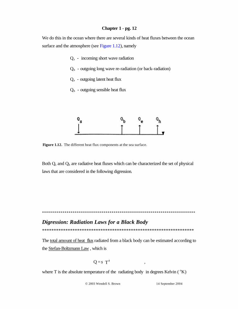
We do this in the ocean where there are several kinds of heat fluxes between the ocean

surface and the atmosphere (see Figure 1.12), namely

Qs - incoming short wave radiation

Qb - outgoing long wave re-radiation (or back-radiation)

Qe - outgoing latent heat flux

Qh - outgoing sensible heat flux

Both Qs and Qb are radiative heat fluxes which can be characterized the set of physical

laws that are considered in the following digression.

***************************************************************************

Digression: Radiation Laws for a Black Body *****************************************************************

The total amount of heat flux radiated from a black body can be estimated according to

the Stefan-Boltzmann Law , which is

where T is the absolute temperature of the radiating body in degrees Kelvin ( oK)

Figure 1.12. The different heat flux components at the sea surface.

T = Q 4σ ,

Chapter 1 - pg. 13


which is

and s is the Stefan-Boltzmann constant with a value of

The maximum wavelength at which the heat flux is radiated from a body can be

estimated according the Wien Displacement Law, which is

where λmax is the wavelength of the peak of the energy spectrum as shown in Figure

1.13.

Figure 1.13. The family of energy spectra for radiation leaving bodies of differing absolute temperatures. The Wien Displacement Law (dashed line) defines the wavelengths (? max) associated with the peaks of different spectra. ***************************************************************************

RADIATIVE HEAT FLUX COMPONENTS

The nature of solar and long wave radiation heat fluxes are considered in terms of the

Stefan-Boltzmann and the Wien Displacement (W-D) radiation laws.

Solar Radiation (Qs): The effective surface temperature of the sun is 5800oC. So

according to the W-D law, its characteristic wavelength is microns .540 = maxλ

(1 micron = µ = 10-6 m), with 99% of the energy at wavelengths λ < 4µ. Thus Qs is

273.15 + C =K °° ;

Ksec--cmcal/ 10 x 1.36 = 42-12 °σ .

K, cm 10 x2.9 = T -1max °λ

Chapter 1 - pg. 14


short wave radiation (typically 1.54 x 103 cal/cm2/sec) impinging on the Earth. This

quantity is sometimes referred to as solar insolation.

Back Radiation (Qb): The Earth also radiates energy back into space, although its

absolute temperature is much lower that that of the sun. The effective surface

temperature of the Earth is 290 oK. So according to W-D microns10 = maxλ , with

90% of the energy in the 3 to 80µ wavelength band. Thus Qb departs from the Earth’s

surface as long wave radiation. The the typical net oceanic Qb value is 0.96 x 10-2

cal/cm2/sec, depending on sea surface temperature as well as the water vapor content

of the air above.

NON-RADIATIVE HEAT FLUX COMPONENTS

Latent and sensible heat fluxes are due to complex air-sea interaction processes and are

estimated using empirically-derived bulk formula based on experimental observations.

Latent Heat Flux (Qe): Heat, drawn from the local ocean environment, is required to

evaporate water - that is provide enough energy to convert water molecules at the

surface from liquid to gas ...and thus break away from the ocean surface. Latent heat

flux is associated with this process and can be estimated by

F is difficult to measure, so it is usually estimated from the “bulk relation”

F, x L = Qe

where F is the mass flux of water evaporated from the sea surface and L (cal/gm)

is the latent heat of sea water

C)].(T .52 - [596 = L °s

which depends on sea surface temperature Ts .

Chapter 1 - pg. 15


where W (m/sec) is the wind speed at 10 m elevation, es (millibars; mb) is the

saturated water vapor pressure at the sea surface temperature Ts (es = 0.98 x the

saturated vapor pressure of distilled water ed -shown in Figure 1.14); ea (mb) is the

water vapor pressure at 10 m above the sea surface based on measured (a) air

temperature Ta and (b) relative humidity RH. Estimating water vapor pressure and

RH are addressed in the following digression.

******************************************************************

Digression - Water Vapor Pressure and Relative Humidity

******************************************************************

Water vapor pressure (or partial pressure) is the portion of the total air pressure

caused by the water vapor. The phase diagram for water (Figure 1.14) relates the

saturated vapor pressure to temperature.

Figure 1.14. Phase diagram showing distilled water vapor pressure ed. The line dividing liquid and

vapor is the saturated water vapor pressure.

Relative Humidity (RH) is the ratio of the water vapor pressure of a parcel of air ea to

, W )e - e.014( )day-cm

gm F( as2

=

20

10

0 -40 -20 0 20

Temp (°C)

water vapor pressure (mb)

vapor

liq

solid

Chapter 1 - pg. 16


the saturated vapor pressure eas at the same specified temperature or

as

a

ee

RH =

*****************************************************************

Sensible Heat Flux: Qh, is the combined transfer of heat due to conduction and

forced convection. It can be estimated using measured quantities and the Bowen ratio,

R, according to

where Ts, es are at sea surface values and Ta, ea are values at 10 m elevation

respectively.

HEAT BUDGET OF THE OCEAN In considering the heat budget of the ocean, the sources and sinks of heat flux must be identified.

Sources:

Qs; short wave radiation from sun and diffuse skylight

Qb; long wave radiation from the atmosphere

Qh; sensible heat transfer from the atmosphere by conduction

Qe; latent heat transfer by water condensation on the sea surface

Sinks:

Qb; long wave radiation loss from the sea surface

, e - eT - T 0.64

QQ

= Ras

as

e

h =

Chapter 1 - pg. 17


Qh; sensible heat loss by conduction

Qe; latent heat loss through evaporation of surface water The relatively complicated picture of incoming and outgoing heat fluxes (Figure 1.15).

represents an annual- and global averaged picture in which all heat fluxes are expressed

as a percentage of the total incoming solar heat flux.

Notes:

(1) Only about ½ of the incoming solar radiation reaches the sea surface

and only ½ of that directly from the sun.

(2) Only 5% of the long wave radiation leaving the sea surface escapes

directly to space. The rest is absorbed by the H2O/CO2 rich

atmosphere; 114% vs. 16% due to short wave solar radiation.

(3) The atmosphere reradiates a significant proportion of the long wave (or

infrared) radiation back to the sea surface where it is absorbed and

reradiated.

Figure 1.15. The mean annual radiation and heat balance of the atmosphere, relative to 100 units

Chapter 1 - pg. 18


of incoming solar radiation, based on satellite measurements and conventional observations. (Tolmazin, 1985)

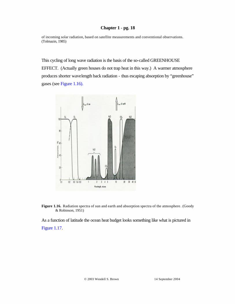
This cycling of long wave radiation is the basis of the so-called GREENHOUSE

EFFECT. (Actually green houses do not trap heat in this way.) A warmer atmosphere

produces shorter wavelength back radiation - thus escaping absorption by “greenhouse”

gases (see Figure 1.16).

Figure 1.16. Radiation spectra of sun and earth and absorption spectra of the atmosphere. (Goody

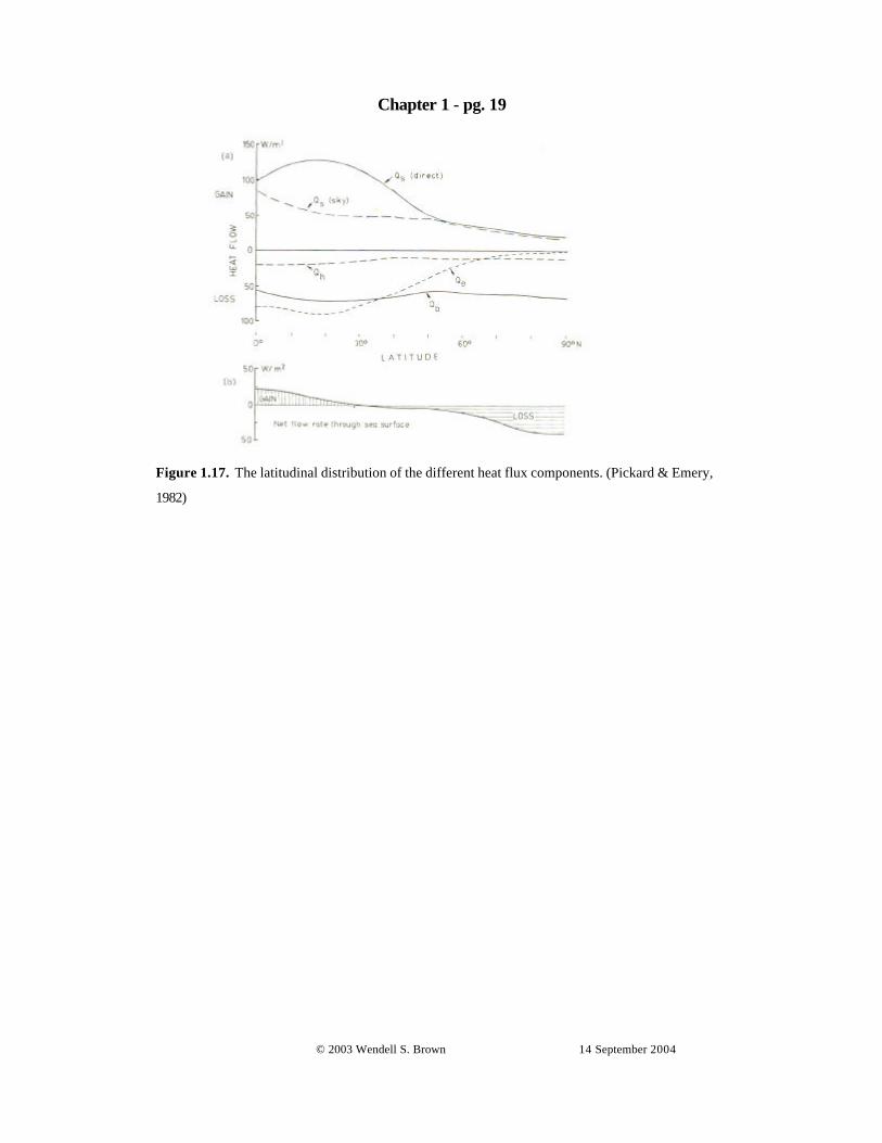
& Robinson, 1951) As a function of latitude the ocean heat budget looks something like what is pictured in

Figure 1.17.

Chapter 1 - pg. 19


Figure 1.17. The latitudinal distribution of the different heat flux components. (Pickard & Emery,

1982)

Chapter 1 - pg. 20


The ocean, like the earth as a whole, also has a surplus of heat in the equatorial regions

and a deficit in the polar regions. The heat surplus must be transported away from the

equatorial zones by ocean currents to achieve the local balance. The amount of heat

transported at each latitude can be determined by considering a latitudinal band of

ocean between latitude lines as shown in Figure 1.18.

The corresponding heat balance for a particular latitude band is

Since on average T∆ ~ 0, Qtrans can be determined from the distributions of Qs, Qe,

Qb, Qh as shown in Figure 1.17. Thus we can derive the distribution of the poleward

Figure 1.18. Schematic for estimating net meridional heat transport in the 10oN to 20oN latitudinal band.

. Q + Q + Q = QQ = Q where

, tT

h Cp = Q - Q - Q

hnet enet bout

totalsin

transoutin ∆∆

∆ρ

Chapter 1 - pg. 21


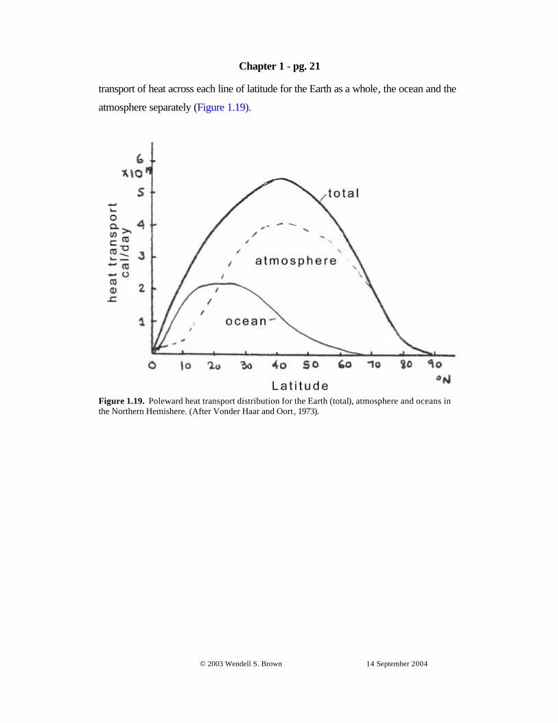
transport of heat across each line of latitude for the Earth as a whole, the ocean and the

atmosphere separately (Figure 1.19).

Figure 1.19. Poleward heat transport distribution for the Earth (total), atmosphere and oceans in the Northern Hemishere. (After Vonder Haar and Oort, 1973).

Chapter 1 - pg. 22


Chapter 1 - PROBLEMS

Chapter 1 - pg. 23


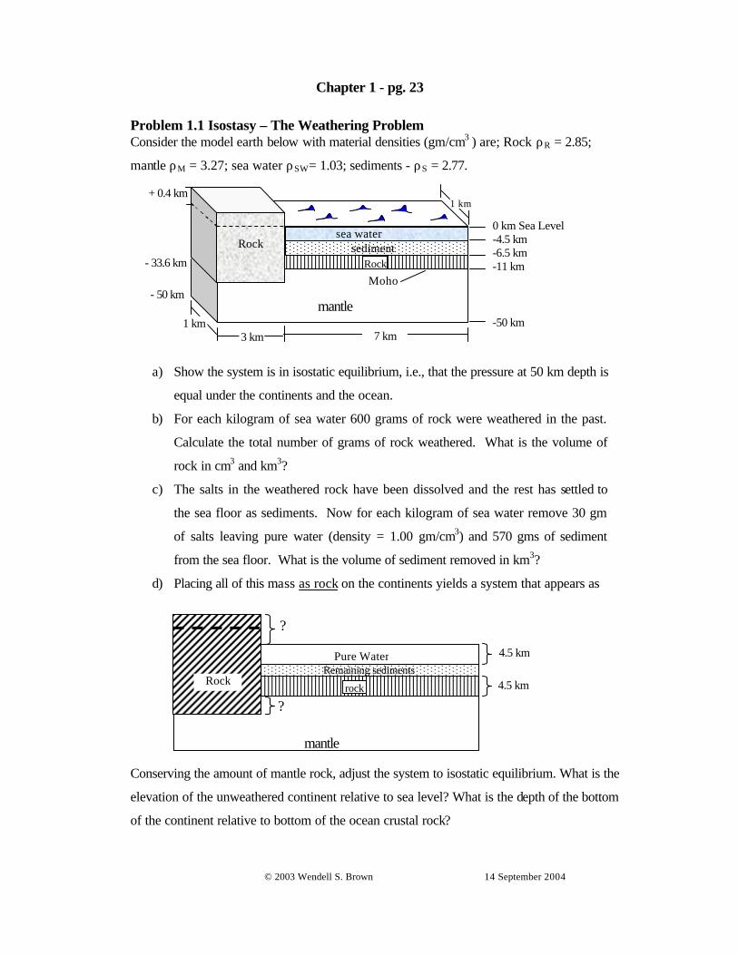
Problem 1.1 Isostasy – The Weathering Problem Consider the model earth below with material densities (gm/cm3 ) are; Rock ρR = 2.85;

mantle ρM = 3.27; sea water ρSW= 1.03; sediments - ρS = 2.77.

a) Show the system is in isostatic equilibrium, i.e., that the pressure at 50 km depth is

equal under the continents and the ocean.

b) For each kilogram of sea water 600 grams of rock were weathered in the past.

Calculate the total number of grams of rock weathered. What is the volume of

rock in cm3 and km3?

c) The salts in the weathered rock have been dissolved and the rest has settled to

the sea floor as sediments. Now for each kilogram of sea water remove 30 gm

of salts leaving pure water (density = 1.00 gm/cm3) and 570 gms of sediment

from the sea floor. What is the volume of sediment removed in km3?

d) Placing all of this mass as rock on the continents yields a system that appears as

Conserving the amount of mantle rock, adjust the system to isostatic equilibrium. What is the

elevation of the unweathered continent relative to sea level? What is the depth of the bottom

of the continent relative to bottom of the ocean crustal rock?

Rock sea water

sediment Rock

0 km Sea Level -4.5 km -6.5 km -11 km

mantle

Moho

-50 km

1 km + 0.4 km

- 33.6 km

- 50 km

7 km 1 km

3 km

Rock rock

mantle

Pure Water Remaining sediments

?

?

4.5 km

4.5 km

Chapter 1 - pg. 24


Problem 1.2 Ocean Volume

Given that (a) approximately 70% of the Earth is covered by the oceans, (b) the

mean depth of the world’s oceans is approximately 4000 m; and (c) the mean

radius of the Earth is 6000 km., calculate the percentage of the Earth's volume that

is comprised by the oceans. Show all of your work including a diagram of the

problem.

Chapter 1 - pg. 25


Problem 1.3 Solar Heating – The Greenhouse Effect (a) The sun (radius RS) radiates energy uniformly in all directions at a temperature

TS. If a spherical planet of radius R is at a distance d from the sun, how much

energy does it intercept in terms of TS, RS, R, d and the Stephan-Boltzmann

constant σ ?

(b) Suppose the planet is perfectly heat conducting and is black so that it is uniform

temperature. If the planet radiates away the same amount of energy that it

receives from space, then what must its temperature be in terms of the variables

in part (a)? Now compute this temperature assuming the planet is the Earth

using

TS = 5800°K d = 150 x 106 km RS = 6.9 x 105 km R = 6371 km (c) Suppose 1/2 of the solar heat flux is reflected from the Earth and 1/2 is

absorbed and then re-radiated. Then what would the Earth’s temperature T be?

d) Explain why the Earth's surface is warmer than the temperature in part (c). e) Suppose only 40% of the radiation radiated by the Earth in case (c) can escape.

What is the temperature at the surface necessary for a radiation balance? Suppose by adding CO2 to the atmosphere, the window opening decreases by 2% so that only 39% of the radiation can escapes. What is T under that scenario?

Chapter 1 - pg. 26


Problem 1.4 Air-Sea Heat Transfer

Consider the situation depicted in the figure above where the generally cold dry wind

blows offshore along the coast of Maine during the winter. An offshore weather buoy

measures the air temperature, Ta, the wind speed, W, the relative humidity, RH, and the

air pressure, Pa, at an elevation of 10m. In addition, a radiometer (chapter 6 in Pickard) is

used to provide the net radiative heat flux to the sea surface (Qs-Qb). An array of

thermistors (black dots) are attached to the mooring line of the weather buoy to measure

water column temperature time series, which are averaged to obtain the average

temperature profile (shown to the right) for the day in question. Given the daily averaged

values of Ta = -10°C, W = 20 ms-1, RH = 0.30, and Qs-Qb = 100 cal/cm2/day, Pa = 1000

mb and the assumption that the saturated water vapor pressure over distilled water ed, can

be expressed as

(a) What is the average amount of water (per unit surface area) evaporated this day? What

is the latent heat flux associated with this mass transfer?

(b) What is the average sensible heat flux during this day?

(c) What is the average net heat flux from the sea surface during this day?

(d) Assume the upper 25 m of the ocean is well mixed and at 10°C. If the same amount of

heat in (c) were to be transferred each successive day and the upper 25 meters of the

ocean were to remain well mixed, what would be the water temperature after three days?

(e)Assume that water density is determined solely by temperature. What do you expect

would happen to the water column if this cooling process were to continue?

Weather Buoy 10 m

100 m

Ta, W, RH, Qs-Qb 0

25

50

75

100

5 10

T(°C)

C0T C15-for 6.1 C)T(0.32 (mb)e and

C15 T 0for 6.1 C)T(10.6(mb)e

d

d

°≤≤°+°×=

°≤≤°+°×=

Chapter 1 - pg. 27


Problem 1.5 Daily Heating - Ocean

a) Suppose the heat flux at the surface of the ocean is 1/4 ly/min. What is the

change in temperature if this heating continues through 12 hours and is distributed

through the upper 10 meters? -- upper 100 meters?

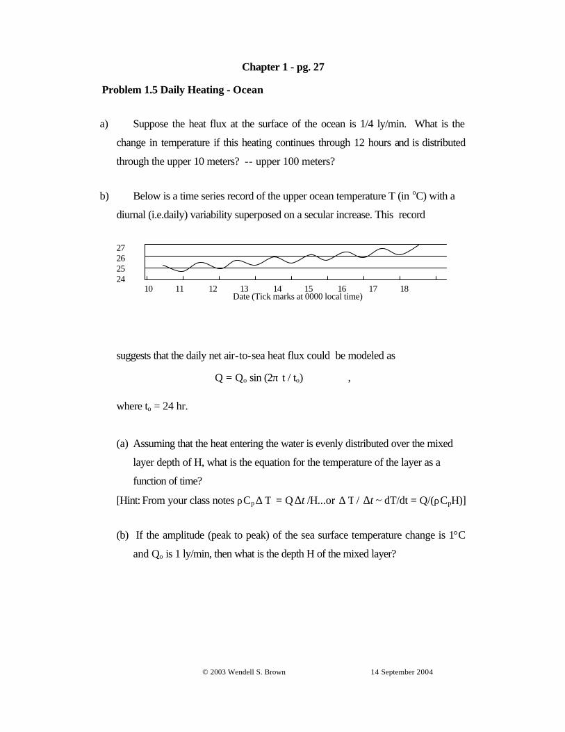
b) Below is a time series record of the upper ocean temperature T (in oC) with a

diurnal (i.e.daily) variability superposed on a secular increase. This record

Date (Tick marks at 0000 local time)

suggests that the daily net air-to-sea heat flux could be modeled as

Q = Qo sin (2π t / to) ,

where to = 24 hr.

(a) Assuming that the heat entering the water is evenly distributed over the mixed

layer depth of H, what is the equation for the temperature of the layer as a

function of time?

[Hint: From your class notes ρCp T∆ = Q t∆ /H...or T∆ / t∆ ~ dT/dt = Q/(ρCpH)]

(b) If the amplitude (peak to peak) of the sea surface temperature change is 1°C

and Qo is 1 ly/min, then what is the depth H of the mixed layer?

27 26 25 24

10 11 12 13 14 15 16 17 18

CHAPTER 1 - GEOPHYSICAL PERSPECTIVE - UMass D · CHAPTER 1 - GEOPHYSICAL ... Figure 1.3 (right) A...

Documents

Transcript of CHAPTER 1 - GEOPHYSICAL PERSPECTIVE - UMass D · CHAPTER 1 - GEOPHYSICAL ... Figure 1.3 (right) A...