Chapter 1 General-Equilibrium Modeling using GAMS · PDF file1 Chapter 1 General-Equilibrium...

1

Chapter 1

General-Equilibrium Modeling using GAMS and MPS/GE: Some Basics

This chapter begins a tutorial on applied general-equilibrium modeling using the specific

software of GAMS and MPS/GE. Before plunging into things, I want to let you know what I will

not cover and what you need to know before continuing.

First, I will not provide a detailed tutorial on GAMS notation and syntax. For these you

can consult the GAMS web site: www.gams.com. Click on documentation, and then on GAMS -

A User’s Guide. This will give you a lot of the basics you need to know. Unfortunately, this

guide is badly out of date and focuses entirely on optimization problems, whereas applied GE

modeling generally involves solving square systems of equations and inequalities. But the user’s

guide will give you the syntax and notation as I indicated. Try going through chapters 2 and 3

before continuing with this tutorial. Hopefully, sometime soon we will try to rewrite the user’s

guide.

Second, you will need to consult the GAMS web site for a copy of the software. I believe

that a demonstration copy is currently provided for free, but this can change of course. Older

versions of the software require the use of an external editor. You best bet for starting is to just

use the DOS editor used under the DOS prompt. You could of could use a word processor and

save your program each time as an ascii text file, but this is clumsy, awkward, and time

consuming.

Again, consult the user’s guide for how to actually run a program and find and view the

output. This set of notes is limited, I am afraid, to actually formulating applied problems into

code and it is beyond the scope of my time and patience to describe and teach that which

logically comes first. The latter needs improvement over what is currently on the web site, but I

will have to leave that to others.

James R. Markusen

Boulder, February 2002

2

1. Introduction to applied general-equilibrium modeling

This is a set of notes to introduce you to applied general-equilibrium modeling and

software used to analyze applied GE problems. First some general comments about general-

equilibrium modeling.

There are many models which are portrayed by their authors’ as “general equilibrium”.

The term assumes different meanings in different fields, so it is probably a good idea to begin

with a definition of what this means. When we say general equilibrium, we are normally

thinking of models which have the following characteristics.

(1) Multiple interacting agents

(2) Individual behavior based on optimization

(3) Most agent interactions are mediated by markets and prices

(4) Equilibrium occurs when endogenous variables (e.g., prices) adjust such that

(i) agents, subject to the constraints they face, cannot do better by altering their

behavior

(ii) markets (generally, not always) clear so, for example, supply equals demand in

each market.

General-equilibrium theory in economics is often quite abstract. A usual introductory

formulation consists of a set of markets for goods and factors of production. Agents, which are

typically labeled consumers and firms, optimize subject to the constraints they face such as

technologies and budget constraints. These optimizations then lead to excess demand functions

for each good and factor. Equilibrium is then obtaining by finding a set of prices such that all

excess demands are zero. General-equilibrium theory is generally focused on abstract issues

such as proving that a set of equilibrium prices and hence equilibrium itself exists.

While this is an important task, the theorists rarely bother with analyzing what those

equilibrium prices are or how they are related to underlying features of the economy such as

preferences, technologies and so forth. And it follows that the abstract theory is of little or no

use in answering questions about how changes in policies such as taxes or tariffs influence the

equilibrium. Some progress can be made in special theoretical models such as the Heckscher-

Ohlin model of international trade. In this model, the direction of trade can be related to

underlying technologies and factor endowments, and the effects of policies such as tariffs on

welfare and the distribution of income among factor owners (the Stolper-Samuelson theorem)

can be derived.

Yet even in the analytical Heckscher-Ohlin model, two problems persist. First, the results

3

are “qualitative”; e.g., they give us the signs of comparative-statics derivatives or tell us that

some elasticity is greater than one. But analytical results cannot be much more precise than that.

Second, almost all results are only unambiguous in a version of the model in which there are two

goods, two factors, two countries and consumers everywhere have identical and homogeneous

preferences over goods. Three goods, three factors, three countries or two distinct consumer

groups create problems that cause the elegant results of Heckscher-Ohlin to collapse.

Applied general-equilibrium modeling is the way around these difficulties, such that the

concept of general-equilibrium actually becomes useful for analyzing real economies and real

policies. Any number of good, factors, household types, and countries may be included. While

the field started out with the assumptions of constant returns to scale and perfect competition in

all production activities, we have learned how to incorporate scale economies and imperfect

competition. We have learned how to include complex tax structures, public goods, externalities,

and “rationing constraints” such as price controls or quotas that prevent markets from clearing.

Naturally, there is a price to be paid from the theorist’s point of view. We have to assume

specific functional forms for preferences, production functions, and so forth. Many parameters

of these functions can be drawn from published data or estimated with econometrics, but others

remain educated guess work. This exercise draws criticism from both theorists and

econometricians alike, but in the end applied GE modeling delivers answers to policy questions,

however imprecise those answers might be.

What exactly is an applied GE model? It begins by following theory: an economy and the

equilibrium conditions for that economy are translated into a mathematical formulation. General

equilibrium is then represented as the solution to a well-defined mathematical problem. More

specifically, there are two general ways of formulating this mathematical problem. The first is to

model the economy as an optimization or programming problem. This tend to be the first way a

student of economics would approach the problem, since optimization and optimization

techniques are a fundamental part of the theory of the consumer and the theory of the firm. Thus

general equilibrium could be thought of as the solution to a big linear or non-linear programming

problem, in which some objective function is maximized or minimized subject to a set of

constraints.

It turns out that representing equilibrium as the solution to an optimization problem

becomes awkward when there are several households or countries. What is it that should be

optimized? There is no clear objective function to optimize. The second way of approaching the

problem follows from formal theory. Individual optimizing behavior and decisions of consumers

and firms are embedded in functions describing the agents’ choices in response to the values of

variables facing them. So, for example, we use individual optimization to derive demand and

supply functions that describe how consumers and firms will react to prices, taxes, and other

variables.

Once we have done this, finding general-equilibrium is reduced to finding the solution to

4

a square system of n equations in n unknowns. Individual behavior and optimization are

embedded in those n equations. That is the approach we take here. An applied general-

equilibrium model is a square system of n equations in n unknowns that is formulated in a

fashion that permits a numerical solution by computational techniques, finding the actual values

of the endogenous variables for given values of exogenous parameters. Endogenous variables

include outputs, prices, trade volumes and so forth. Exogenous parameters include preferences,

technologies, factor endowments and so forth.

As we will see shortly, the software we use permits a very important generalization of this

notion of solving a square system of equations. For many economic problems, equilibrium may

involve some goods not being produced or some possible trade links not being actively used. We

really would like to formulate the general-equilibrium model as a system of weak inequalities,

with each inequality associated with a particular non-negative variable such as a price or

quantity. If a particular weak inequality holds as an equation, then the associated variable is

strictly positive. If it holds as a strict inequality, then the associated variables is zero.

An example of this for a competitive model is the requirement that, in equilibrium, the

profits from a given production activity must be non-positive. The associated variable to this

inequality is the output level of that activity. In equilibrium, the weak inequality may hold as a

strict equality, in which case there is positive output. If it holds as a strict inequality, (potential)

profits from that production activity are negative, and no output is produced.

Thus we will formulate a general equilibrium model as a square system of weak

inequalities, each with an associated non-negative variable. This is referred to as a

complementarity problem in mathematics, and the associated variables are referred to as

complementary variables.

Software other than that used here (GAMS and MPS/GE) generally do not allow the user

to solve complementarity problems, greatly limiting model formulation and the range of

comparative statics questions analyzed by the modeler.

5

2. Steps in Applied General-Equilibrium Modeling

Here are the “normal” steps in applied general-equilibrium modeling.

(1) Specify dimensions of the model.

• Numbers of goods and factors

• Numbers of consumers

• Numbers of countries

• Numbers of active markets

(2) Chose functional forms for production, transformation, and utility functions; specification

of side constraints.

• Includes choice of outputs and inputs for each activity

• Includes specification of initially slack activities

(3) Construct micro-consistent data set.

• Data satisfies zero profits for all activities, or if profits are positive, assignment of

revenues

• Data satisfies market clearing for all markets

(4) Calibration – parameters are chosen such that functional forms and data are consistent.

• By “consistent” we mean that the data represent a solution to the model

(5) Replication – run model to see if it reproduces the input data.

(6) Counter-factual experiments.

Steps (3) and (4) are not strictly speaking necessary. The software can be used for pure

simulation analysis, in which there initially is no data.

However, in learning the software, it is very valuable to start by writing down a micro-consistent

data set and then transform that into code such that the solution to the model reproduces the

initial data.

6

Let’s now turn to a concrete example of a simple general-equilibrium model.

Example M1: 2-good, 2-factor closed economy with fixed factor endowments, one

representative consumer.

Take a very simply economy, two sectors (X and Y), two factors (L and K), and one

representative consumer (utility function W). L and K are in inelastic (fixed) supply, but can

move freely between sectors. px, py, pl, and pk are the prices of X, Y, L and K, respectively. I is

consumer’s income and pw will be used later to denote the price of one unit of W. These are the

equations of the model.

(1) X X (Lx, K

x)

(2) Y Y (Ly, K

y)

(3) L Lx

Ly

(4) K Kx

Ky

(5) W W(X , Y )

(6) I plL p

kK p

xX p

yY

___________________________________________________________

How do we find equilibrium, which in this case is a set of prices, and factor allocations to the

two sectors? Many economists’ first reaction would be to formulate equilibrium as the solution

to an optimization problem. Equilibrium could be solved for by a constrained optimization

problem: Max (5) subject to the constraints (1), (2), (3), (4), and (6).

While this would work, the usefulness of this approach breaks down quickly as the model

becomes more complicated. Suppose, for example, there are two different consumer types with

different preferences and different factor endowments. What do we maximize? You could

maximize the utility of one consumer subject to an arbitrary fixed level of the utility of the other

consumer, exploiting the first theorem of welfare economics. But unless you are extraordinarily

lucky, the solution will give each consumer an implied expenditure level which is not equal to

the consumer’s income. Thus there is an inconsistency in the proposed solution.

7

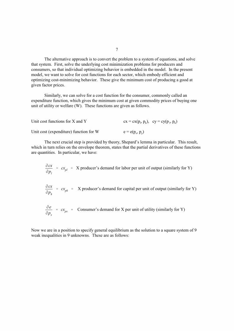
The alternative approach is to convert the problem to a system of equations, and solve

that system. First, solve the underlying cost minimization problems for producers and

consumers, so that individual optimizing behavior is embedded in the model. In the present

model, we want to solve for cost functions for each sector, which embody efficient and

optimizing cost-minimizing behavior. These give the minimum cost of producing a good at

given factor prices.

Similarly, we can solve for a cost function for the consumer, commonly called an

expenditure function, which gives the minimum cost at given commodity prices of buying one

unit of utility or welfare (W). These functions are given as follows.

Unit cost functions for X and Y cx = cx(pl, pk), cy = cy(p l, pk)

Unit cost (expenditure) function for W e = e(px, py)

The next crucial step is provided by theory, Shepard’s lemma in particular. This result,

which in turn relies on the envelope theorem, states that the partial derivatives of these functions

are quantities. In particular, we have:

X producer’s demand for labor per unit of output (similarly for Y)cx

pl

cxpl

X producer’s demand for capital per unit of output (similarly for Y)cx

pk

cxpk

Consumer’s demand for X per unit of utility (similarly for Y)e

px

cxpx

Now we are in a position to specify general equilibrium as the solution to a square system of 9

weak inequalities in 9 unknowns. These are as follows:

8

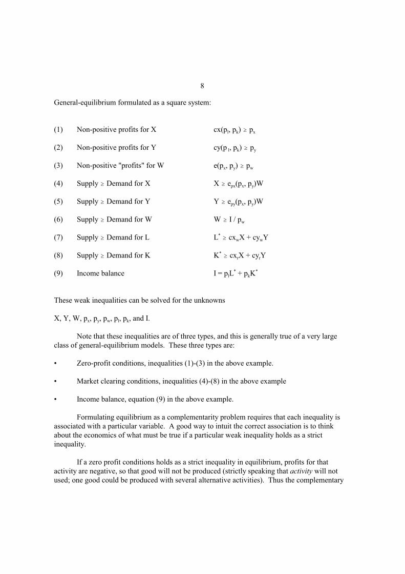
General-equilibrium formulated as a square system:

(1) Non-positive profits for X cx(pl, pk) px

(2) Non-positive profits for Y cy(p l, pk) py

(3) Non-positive "profits" for W e(px, py) pw

(4) Supply Demand for X X epx(px, py)W

(5) Supply Demand for Y Y epy(px, py)W

(6) Supply Demand for W W I / pw

(7) Supply Demand for L L* cxwX + cywY

(8) Supply Demand for K K* cxrX + cyrY

(9) Income balance I = plL* + pkK

*

These weak inequalities can be solved for the unknowns

X, Y, W, px, py, pw, pl, pk, and I.

Note that these inequalities are of three types, and this is generally true of a very large

class of general-equilibrium models. These three types are:

• Zero-profit conditions, inequalities (1)-(3) in the above example.

• Market clearing conditions, inequalities (4)-(8) in the above example

• Income balance, equation (9) in the above example.

Formulating equilibrium as a complementarity problem requires that each inequality is

associated with a particular variable. A good way to intuit the correct association is to think

about the economics of what must be true if a particular weak inequality holds as a strict

inequality.

If a zero profit conditions holds as a strict inequality in equilibrium, profits for that

activity are negative, so that good will not be produced (strictly speaking that activity will not

used; one good could be produced with several alternative activities). Thus the complementary

9

variable to a zero-profit condition is a quantity, the activity level. If a market-clearing condition

holds as a strict inequality, supply exceeds demand for that good or factor in equilibrium so its

price must be zero. Thus the complementary variable to a market clearing equation is the price

of that good or factor. The complementary variable to an income balance equation is just the

income of that agent. The correct association of inequalities and unknowns in the square system

is thus:

Inequality Complementary Variable

(1) Non-positive profits for X cx(pl, pk) px X

(2) Non-positive profits for Y cy(pl, pk) py Y

(3) Non-positive "profits" for W e(px, py) pw W

(4) Supply Demand for X X epx(px, py)W px ,

(5) Supply Demand for Y Y epy(px, py)W py

(6) Supply Demand for W W I / pw pw

(7) Supply Demand for L L* cxwX + cywY pl

(8) Supply Demand for K K* cxrX + cyrY pk

(9) Income balance I = plL* + pkK

* I

Now let’s turn to the issue of starting with a micro-consistent data set, a set of numbers

which are in fact consistent with the above problem formulation. That is, let’s start with a set of

numbers that satisfy zero profits, market clearing, and income balance.

The above problems can be thought of as consisting of three production activities, X, Y,

and W, and four markets, X, Y, L, and K.

In what follows, we will represent the initial data for this economy by a rectangular

matrix. This matrix is related to the concept of a “SAM” – social accounting matrix, which is

discussed later. But the term SAM has been used in a rather different sense, so we will just refer

to our rectangular matrix as a “MCM” – micro-consistency matrix.

In the present example, there are two types of columns in the rectangular MCM,

corresponding to production sectors and consumers. In the model outlined above, there are three

production sectors (X, Y and W) and a single consumer (CONS). Rows correspond to markets in

10

the present example. Complementary variables are prices, so we have listed the price variables

on the left to designate rows.

In the MCM, there are both positive and negative entries. A positive entry signifies a

receipt (sale) in a particular market. A negative entry signifies an expenditure (purchase) in a

particular market. Reading down a production column, we then observe a complete list of the

transactions associated with that activity. Here is our matrix of initial values.

Production Sectors Consumers

Markets | X Y W | CONS Row sum

---------------------------------------------------------------------------------------

PX | 100 -100 | 0

PY | 100 -100 | 0

PW | 200 | -200 0

PL | -25 -75 | 100 0

PK | -75 -25 | 100 0

---------------------------------------------------------------------------------------

Column sum 0 0 0 0

A rectangular MCM is “balanced” or “micro-consistent” when row and column sums are

zeros. Positive numbers represent the value of commodity flows into the economy (sales or

factor supplies), while negative numbers represent the value of commodity flows out of the

economy (factor demands or final demands).

With this interpretation, a row sum is zero if the total amount of commodity flowing into

the economy equals the total amount of commodity flowing out of the economy. This is market

clearance, and one such condition applies for each commodity in the model.

Columns in this matrix correspond to production sectors or consumers. A production

sector column sum is zero if the value of outputs equals the cost of inputs. A consumer column

is balanced if the sum of primary factor sales equals the value of final demands. Zero column

sums thus indicate zero profits or “product exhaustion” in an alternative terminology.

Finally, we emphasize that the numbers of the matrix are values, prices times quantities.

The modeler is free as to how to interpret these as prices versus quantities. A good practice is to

choose units so that as many things initially are equal to one as possible. Prices can be chosen as

one, and “representative quantities” for activities can be chosen such that activity levels are also

equal to one (e.g., activity X run at level one produces 100 units of good X). In the case of

taxes, both consumer and producer prices cannot equal one of course, a point we will return to in

a later section.

11

Now we are in a position to adopt functional forms and write an actual GAMS program to

solve this model.

First, we specify this general-equilibrium model as an MCP, writing out all the functions.

We use very simple Cobb-Douglas functions for the three activities. The share parameters for

the functions are given in the data matrix above. Goods in the utility function get equal shares of

0.5. X is capital intensive with capital having a share of 0.75 and labor a share of 0.25. Y is

labor intensive with the opposite ordering of shares.

While we will not go into detail about GAMS syntax here, a few final points with respect to the

actual program follows.

(1) The opening line $TITLE is not necessary, but used to the model in the listing (output)

file.

(2) $ONTEXT.....$OFFTEXT is a way of designating a block of comments, to be ignored by

GAMS. In this case, we put our data matrix inside this block, meaning it is not actually

used in the computation.

(3) A text line can also be preceded by a *. GAMS ignores any line beginning with a *.

(4) We declare the parameter names, then assign them values (note where semi-colons do

and do not go).

(5) Next we declare positive variables and then equation names. We write out the equation

names in the syntax shown [equation name], then the equation itself ending with a semi-

colon. Note the use of the reference quantities such as “100”, “75 ” etc. in the equations.

This will ensure that the activity levels will be X = Y = W = 1 in the initial solution to the

model.

(6) Note that GAMS was written to use greater-than-or-equal-to syntax (=G=). Also note

that we have avoided having variables in denominators, since if a variable (even

temporarily during the execution of the algorithm) has a value of zero, this causes a

divided by zero problem and may crash the solver.

(7) Then the model is specified, and we chose a numeraire (recall from theory that only

relative prices are determined). Here we choose utility as the numeraire, so that factor

prices are then real values in terms of utility. The notation is PW.FX, “FX” for “fixed”.

(5) Before the solve statement, we are going to help the solver by giving starting values for

the variables. The syntax is, for example X.L, where the “L” stands for “level”. Default

values are zero, and in non-linear problems it is very helpful and indeed sometimes

necessary to help the solver with some initial guesses. We constructed this problem

12

knowing the answer, so I give those values as .L values.

(6) Finally, the solve statement.

Now we are ready to go. After the first solve statement, we do two counterfactual experiments.

The first sets a tax of 0.50 on the inputs to X production. Then we have a second solve

statement. Finally, we remove the tax and double the labor endowment of the economy.

“TX” is a parameter which sets the tax, and “LENDOW” is a multiplier on the initial labor

endowment.

13

$TITLE Model M1_MCP: Closed 2x2 Economy - An Introduction to the Basics

$ONTEXT

This is the exact same model as M1_MPS.GMS but uses the MCP format.

Production Sectors Consumers Markets | X Y W | CONS ------------------------------------------------------ PX | 100 -100 | PY | 100 -100 | PW | 200 | -200 PL | -25 -75 | 100 PK | -75 -25 | 100 ------------------------------------------------------

$OFFTEXT

PARAMETERS

TX Ad-valorem tax rate for X sector inputs LENDOW Labor endowment multiplier;

TX = 0;LENDOW = 1;

POSITIVE VARIABLES X Y W PX PY PW PL PK CONS;

EQUATIONS PRF_X Zero profit for sector X PRF_Y Zero profit for sector Y PRF_W Zero profit for sector W (Hicksian welfare index)

MKT_X Supply-demand balance for commodity X MKT_Y Supply-demand balance for commodity Y MKT_L Supply-demand balance for primary factor L MKT_K Supply-demand balance for primary factor L MKT_W Supply-demand balance for aggregate demand

14

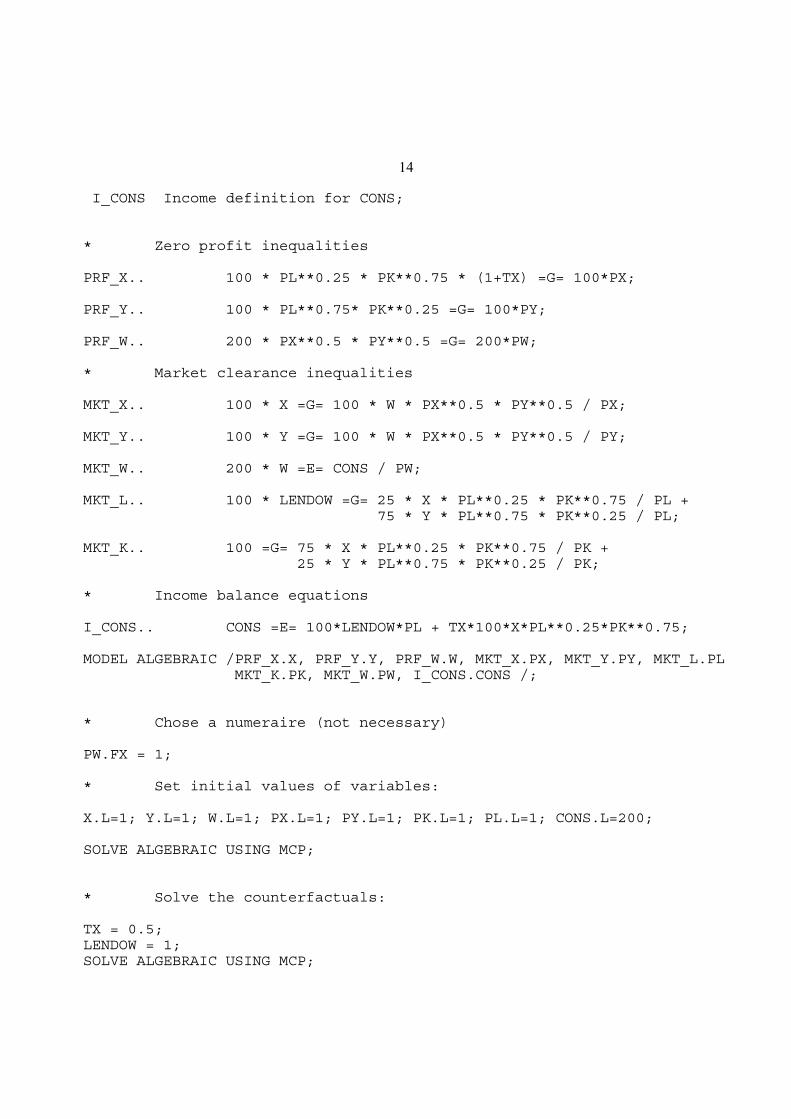
I_CONS Income definition for CONS;

* Zero profit inequalities

PRF_X.. 100 * PL**0.25 * PK**0.75 * (1+TX) =G= 100*PX;

PRF_Y.. 100 * PL**0.75* PK**0.25 =G= 100*PY;

PRF_W.. 200 * PX**0.5 * PY**0.5 =G= 200*PW;

* Market clearance inequalities

MKT_X.. 100 * X =G= 100 * W * PX**0.5 * PY**0.5 / PX;

MKT_Y.. 100 * Y =G= 100 * W * PX**0.5 * PY**0.5 / PY;

MKT_W.. 200 * W =E= CONS / PW;

MKT_L.. 100 * LENDOW =G= 25 * X * PL**0.25 * PK**0.75 / PL + 75 * Y * PL**0.75 * PK**0.25 / PL;

MKT_K.. 100 =G= 75 * X * PL**0.25 * PK**0.75 / PK + 25 * Y * PL**0.75 * PK**0.25 / PK;

* Income balance equations

I_CONS.. CONS =E= 100*LENDOW*PL + TX*100*X*PL**0.25*PK**0.75;

MODEL ALGEBRAIC /PRF_X.X, PRF_Y.Y, PRF_W.W, MKT_X.PX, MKT_Y.PY, MKT_L.PL MKT_K.PK, MKT_W.PW, I_CONS.CONS /;

* Chose a numeraire (not necessary)

PW.FX = 1;

* Set initial values of variables:

X.L=1; Y.L=1; W.L=1; PX.L=1; PY.L=1; PK.L=1; PL.L=1; CONS.L=200;

SOLVE ALGEBRAIC USING MCP;

* Solve the counterfactuals:

TX = 0.5;LENDOW = 1;SOLVE ALGEBRAIC USING MCP;

15

TX = 0;LENDOW = 2;SOLVE ALGEBRAIC USING MCP;

This file is saved in the relevant directory as M1_MCP.GMS, although you can use any name you want, it

doesn’t have to correspond to the model name.

At the DOS prompt, >, type GAMS M1_MCP. This command runs the model.

The output or listing file will automatically be written to the same directory, with name M1_MCP.LST.

In the listing file, we will see the following information, along with a statement that the solution is normal

and optimal. We will not go into a long explanation here, but rather just focus on the solution values. The

list of 1.000 indicates we successfully reproduced our benchmark data as an equilibrium, since we chose

units such that this would be the case.

16

LOWER LEVEL UPPER MARGINAL

---- EQU PRF_X . . +INF 1.000---- EQU PRF_Y . . +INF 1.000---- EQU PRF_W . . +INF 1.000---- EQU MKT_X . . +INF 1.000---- EQU MKT_Y . . +INF 1.000---- EQU MKT_L -100.000 -100.000 +INF 1.000---- EQU MKT_K -100.000 -100.000 +INF 1.000---- EQU MKT_W . . . 1.000---- EQU I_CONS . . . 200.000

PRF_X Zero profit for sector X PRF_Y Zero profit for sector Y PRF_W Zero profit for sector W (Hicksian welfare index) MKT_X Supply-demand balance for commodity X MKT_Y Supply-demand balance for commodity Y MKT_L Supply-demand balance for primary factor L MKT_K Supply-demand balance for primary factor L MKT_W Supply-demand balance for aggregate demand I_CONS Income definition for CONS


---- VAR X . 1.000 +INF .---- VAR Y . 1.000 +INF .---- VAR W . 1.000 +INF .---- VAR PX . 1.000 +INF .---- VAR PY . 1.000 +INF .---- VAR PW 1.000 1.000 1.000 EPS---- VAR PL . 1.000 +INF .---- VAR PK . 1.000 +INF .---- VAR CONS . 200.000 +INF .

Now let’s look at the results for our first counterfactual, in which we place a 50% tax on the inputs to X

production.

************** counterfactual: tax on X inputs


---- VAR X . 0.845 +INF .---- VAR Y . 1.147 +INF .---- VAR W . 0.985 +INF .---- VAR PX . 1.165 +INF .---- VAR PY . 0.859 +INF .---- VAR PW 1.000 1.000 1.000 -16.412---- VAR PL . 0.903 +INF .

17

---- VAR PK . 0.739 +INF .---- VAR CONS . 213.359 +INF .

We see that X production decreases, Y production increases, and welfare falls due to the distortionary

nature of the tax, even though the tax revenue is redistributed back to the consumer. There is also a

redistribution of income between factors. The relative price of capital, the factor used intensively in X falls,

and the relative price of labor rises as resources are shifted to Y production.

In the second counterfactual, we remove the tax, and double the labor endowment of the economy.

***************counterfactual: double labor endowment (zero tax)


---- VAR X . 1.189 +INF .---- VAR Y . 1.682 +INF .---- VAR W . 1.414 +INF .---- VAR PX . 1.189 +INF .---- VAR PY . 0.841 +INF .---- VAR PW 1.000 1.000 1.000 6.617E-11---- VAR PL . 0.707 +INF .---- VAR PK . 1.414 +INF .---- VAR CONS . 282.843 +INF .

Here we see a relative shift to Y, the good using labor intensively, although X production also rises. The

price of X rises relative to Y. The real price of capital, now the scarce factor, rises, and the real price of

labor falls. Although labor has a 50% income share initially, doubling labor supply increases welfare by less

than 50% (it increases W by 41.4%) due to diminishing returns from the presence of the fixed factor capital.

18

3. The MPS/GE subsystem of GAMS

GAMS now include a higher-level language, written by Rutherford, called MPS/GE,

which stands for mathematical programming system for general equilibrium. MPS/GE uses the

MCP solver in GAMS. This higher-level language permits extremely efficient shortcuts for

modelers, allowing us to concentrate on economics rather than coding.

There are several great features of MPS/GE. First, the program has routines for

calibrating and writing all constant-returns CES and CET functions, up to three levels of nesting.

All the modeler has to do is to specify the nesting structure, substitution elasticities in each nest

and a representative point on the function, consisting of output quantities, input quantities and

prices. This point and price vector uniquely determine the function, and MPS/GE then generates

the cost function (or expenditure function). This is not that time and error saving in the simple

simulation models of this book, but it is a wonderful feature for larger models.

Second, and closely related, the form of the data required to specify a CES/CET function

is exactly the data modelers have, so there is a swift and easy move from an accounting matrix as

described in the previous appendix to the calibration of the model.

Third, a lot of market-clearing and income-balance equations are written automatically by

MPS/GE so the modeler doesn’t have to worry about doing so. Fourth, and closely related, a lot

of errors that can occur when a modeler writes out his or her equations cannot occur in MPS/GE.

If there is a tax or markup, for example, the revenues must be assigned to some agent and will be

allocated automatically to that agent by the income-balance properties of the coding. I once

refereed a paper in which the author claimed to have some weird numerical result. It turned out

that the modeler had a tax, but forgot to put the tax revenue in the representative agent’s income

balance equation. That cannot happen in MPS/GE. In short, MPS/GE automatically checks for

and ensures many of the product-exhaustion and income-balance requirements discussed in the

previous section.

In this appendix, I am going to give a short and superficial introduction to the MPS/GE

subroutine of GAMS. I am going to use exactly the same problem as in the previous appendix,

so that you can see the connection. First, a few key words.

SECTOR (ACTIVITY)

Production activities that convert commodity inputs into commodity outputs. The variable

associated with a sector is the activity level.

COMMODITY (MARKETS)

A good or factor. The variable associated with a commodity is its price, not its quantity.

19

CONSUMERS

Individuals who supply factors and receive tax revenues, markups, and pay subsidies. In

imperfectly competitive models, firm owners can be designated as consumers. A government

that receives tax revenue and buys public goods is also designated as a consumer. The variable

associated with a consumer is income from all sources.

AUXILIARY

Additional variables, such as markup formulae or taxes with endogenous values which are

functions of other variables such as prices and quantities. Please note the spelling of auxiliary:

mistakes cause MPS/GE to crash, and you won’t know why.

CONSTRAINT

An equation that is typically used to set the value of an auxiliary variable. In these appendix

programs, constraint equations will be used to set the values of markups, which are auxiliary

variables.

Here is what an MPS/GE program, embedded in a GAMS file, looks like, where the model name

is M1_MCP.

______________________________________________________________

GAMS statements such as declaring sets, parameters, parametervalues, etc.

**** now control is passed to the MPS/GE subsystem ****

$ONTEXT [this tells the GAMS compiler to ignore what follows,but the MPS/GE compiler will recognize the modelstatement that follows and will begin to pay attention]

$MODEL: M1_MCP

Declaration of sectors, commodities, consumers, auxiliaryvariables

Production Blocks

Demand Blocks

Constraint equations

$OFFTEXT [control is passed back to GAMS]

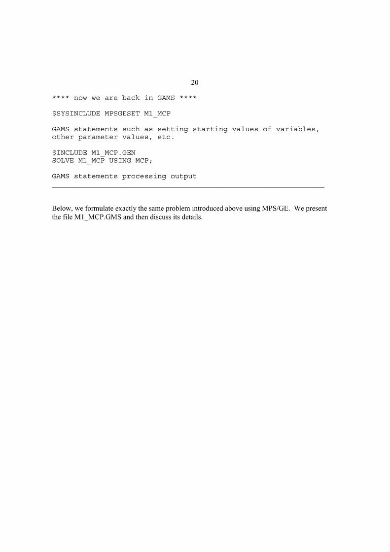
20

**** now we are back in GAMS ****

$SYSINCLUDE MPSGESET M1_MCP

GAMS statements such as setting starting values of variables,other parameter values, etc.

$INCLUDE M1_MCP.GENSOLVE M1_MCP USING MCP;

GAMS statements processing output______________________________________________________________

Below, we formulate exactly the same problem introduced above using MPS/GE. We present

the file M1_MCP.GMS and then discuss its details.

21

$TITLE Model M1_MPS: Closed 2x2 Economy - An Introduction to the Basics

$ONTEXT

This is the exact same model as M1_MCP.GMS but uses the MPS/GE format.


$OFFTEXT

PARAMETERS TX Ad-valorem tax rate for X sector inputs LENDOW Labor endowment multiplier;

TX = 0;LENDOW = 1;

$ONTEXT

$MODEL:M1_MPS

$SECTORS: X ! Activity level for sector X Y ! Activity level for sector Y W ! Activity level for sector W (Hicksian welfare index)

$COMMODITIES: PX ! Price index for commodity X PY ! Price index for commodity Y PL ! Price index for primary factor L PK ! Price index for primary factor K PW ! Price index for welfare (expenditure function)

$CONSUMERS: CONS ! Income level for consumer CONS

$PROD:X s:1 O:PX Q:100 I:PL Q:25 A:CONS T:TX

22

I:PK Q:75 A:CONS T:TX

$PROD:Y s:1 O:PY Q:100 I:PL Q:75 I:PK Q:25

$PROD:W s:1 O:PW Q:200 I:PX Q:100 I:PY Q:100

$DEMAND:CONS D:PW Q:200 E:PL Q:(100*LENDOW) E:PK Q:100

$OFFTEXT

$SYSINCLUDE mpsgeset M1_MPS

PW.FX = 1;

$INCLUDE M1_MPS.GENSOLVE M1_MPS USING MCP;

* Solve the counterfactuals

TX = 0.5;LENDOW = 1;


TX = 0;LENDOW = 2;


23

Now some more details.

(1) Production blocks

The terminology here is a bit confusing, since MPS/GE takes the information in a

production block and generates a cost function, not a production function. But the variable

complementary with a production block (cost function) is an activity level. Let’s take an

example from the above program, adding the price field (discussed shortly).

$PROD:Y s:1 O:PY Q:100 P:1 I:PL Q: 75 P:1 I:PK Q: 25 P:1

First line

Name of activity (Y), value of substitution (here s:1) and transformation elasticities if there are

several outputs. Default elasticity of substitution is 0 (not 1!).

First column

Names of commodity outputs (O:) and inputs (I:).

Second column

Reference commodity quantities (Q:) – used for calibration. Default = 1 if none specified.

Third column

Reference commodity prices (P) – used for calibration. Default = 1 if none specified, which is

why they are omitted in the program above.

MPS/GE then takes this information to construct a cost function and, as a feature of CES

functions, it is globally defined by a single reference point. Think of putting an isoquant labeled

100 units of output, with elasticity of substitution 1, though input points L = 70, K = 30, with

slope PL/PK = 1. That is what MPS/GE does for you. In this simple case, it constructs the cost

function:

100*(PL**.75)*(PK**.25) =G= 100*PY;

The saving from using MPS/GE might not seem like a big deal, but believe me with many inputs,

different prices for all inputs, and an elasticity of substitution of 3.5, it is a huge saving indeed.

One example of the treatment of taxes (others will follow later, including those with

endogenous rates) is in the production block for X.

24

$PROD:X s:1 O:PX Q:100 I:PL Q:25 A:CONS T:TX I:PK Q:75 A:CONS T:TX

The “A” field means “assign” the revenue from tax TX to the agent CONS. Read it as the

statement “assign to agent CONS the revenue from tax rate TX on inputs L and K”.

A utility function is also represented by a production block; that is, utility is a good which

is produced from commodity inputs (including possibly factor inputs such as leisure). Here is the

utility function (W for welfare), in which utility (good PW) is produced from inputs of X and Y.

MPS/GE constructs the underlying expenditure (cost) function.


A consumer’s income constraint is also represented by a “block” in this case called a demand

block. In what follows, the consumer demands the utility good PW (the “D” field), and receives

income from endowments (the “E” fields) of labor and capital.

MPS/GE automatically handles tax revenue or subsidy payments in the background, adding or

subtracting them to the consumer's endowment income.

$DEMAND:CONS D:PW Q:200 E:PL Q:(100*LENDOW) E:PK Q:100

MPS/GE also automatically looks after the market clearing conditions without the modeler

having to worry about specifying these additional equations.

4. Example of how the Q and P fields are used to construct the underlying cost function.

All constant returns CES and CET functions can be completely characterized by a single point

consisting of (1) input quantities (2) output quantities (3) input and output prices, and (4) the

elasticity of substitution or transformation (there may be several levels of substitution

elasticities).

25

MPS/GE constructs the underlying cost function from such a single observation. It is particularly

important to specify the reference prices correctly. Consider the two production blocks:

$PROD: X s:1O:PX Q:100 P:1I:PL Q: 25 P:1I:PK Q: 75 P:1

$PROD: X s:1O:PX Q:100 P:1I:PL Q: 25 P:2I:PK Q: 75 P:0.667

These are both Cobb-Douglas production functions that can produce 100 X from inputs of 25

labor and 75 capital, and in each case the value of the inputs equals the value of the output. But

the isoquant has a different slope through that input combination in the two cases: the marginal

rate of substitution in the first case is one, but 3 in the second case. Thus these are not the same

technologies.

Later, with various taxes, it is important to divide values into price and quantity components

when all prices cannot be normalized to one. Consider the following two production blocks.

$PROD: X s:1O:PX Q:100 P:1I:PL Q: 25 P:1I:PK Q: 75 P:1

$PROD: X s:1O:PX Q:100 P:1I:PL Q: 50 P:0.5I:PK Q: 75 P:1

In both cases, the values of inputs and output are the same, and would appear the same in the data

matrix. But these are not the same functions, the first being a clearly more efficient technology

than the second. While both will have the same share parameters on L and K (0.25 and 0.75

respectively), the first technology will have a higher multiplicative “efficiency” parameter scaling

up the output from given inputs (or scaling down the cost of output at given factor prices).

MPS/GE will automatically calculate this scaling parameter.

More will be said about this when we get to an example with taxes in the benchmark data

shortly.

26

5. Vector syntax for GAMS and MPS/GE.

GAMS has some features that streamline the formulation of the computer code, features

that are immensely useful in large dimension problems in particular. We cannot go through all

the features of GAMS syntax here, students must rely on the GAMS manual itself. But we can

show you what these features are and how they are used.

First, actual numbers need not appear in MCP program equations or in MPS/GE

production and demand blocks.. These can be specified somewhere else in the program or

indeed read from external files.

Second, set notation can be used when convenient, as in cases where there are many

goods, factors, countries or consumers. Combining these two features, data can be specified in

an array or table, and read into the computation program in a straightforward way.

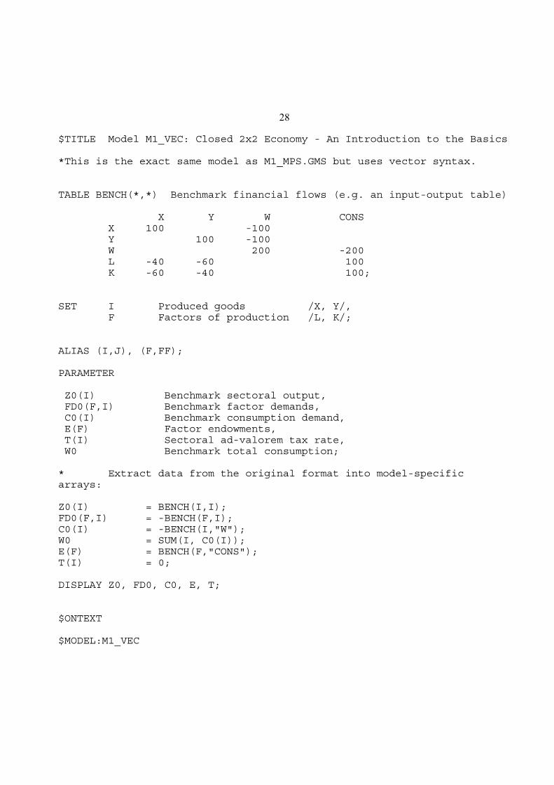
In what follows, we rewrite our basic model from above using these features. We present

first the MPS/GE version and then the MCP version for completeness.

The program begins with the GAMS key word “TABLE”. Now our micro-consistency

matrix is actually going to be used directly in the program to load the values of variables and

parameters. Then we use the GAMS key word “SET”. We use two sets here, the set of goods

(X, Y) and the set of factors (L, K). “ALIAS” is a GAMS key word that allows two different

designators for a given set.

We then declare parameters, and after that parameter assignments are used to extract the

data from the TABLE. Following these assignments of data to parameters, we use a “DISPLAY”

statement, which will write out the values of the parameters in the listing file, so we can do a

quick check that the assignments are correct. Again, you should consult the GAMS manual for a

much more complete description of these operations and definitions (for example the use of “”

when referring to a specific element of a table or set; e.g., BENCH(I, “W”)).

The MPS/GE block follows. Note the absence of any numbers. Consider the production

block:

$PROD:Z(I) s:1 O:PC(I) Q:Z0(I) I:PF(F) Q:FD0(F,I) A:CONS T:T(I)

Two production (cost) functions for two goods using two factors with different factor intensities

and different tax rates across sectors are specified in this extremely parsimonious way.

Following the MPS/GE version, we present the MCP version of the basic model. The

share parameters for the Cobb-Douglas functions are calculated from the data (ALPHA, BETA).

Note also the use of GAMS key words SUM (sum of) and PROD (production of).

27

Note also the use of the alternative set designators, in CMKET(I), for example. If we

have an equation for market I = X, for example, GAMS does not permit us to sum over all values

of I on the right-hand side. But we can sum over the alias J, which is what we do.

In the counterfactuals, note again the use of quotation marks to designate a particular

member of a set.

28

$TITLE Model M1_VEC: Closed 2x2 Economy - An Introduction to the Basics

*This is the exact same model as M1_MPS.GMS but uses vector syntax.

TABLE BENCH(*,*) Benchmark financial flows (e.g. an input-output table)

X Y W CONS X 100 -100 Y 100 -100 W 200 -200 L -40 -60 100 K -60 -40 100;

SET I Produced goods /X, Y/, F Factors of production /L, K/;

ALIAS (I,J), (F,FF);

PARAMETER

Z0(I) Benchmark sectoral output, FD0(F,I) Benchmark factor demands, C0(I) Benchmark consumption demand, E(F) Factor endowments, T(I) Sectoral ad-valorem tax rate, W0 Benchmark total consumption;

* Extract data from the original format into model-specificarrays:

Z0(I) = BENCH(I,I);FD0(F,I) = -BENCH(F,I);C0(I) = -BENCH(I,"W");W0 = SUM(I, C0(I));E(F) = BENCH(F,"CONS");T(I) = 0;

DISPLAY Z0, FD0, C0, E, T;

$ONTEXT

$MODEL:M1_VEC

29

$SECTORS: Z(I) ! Commodity production index W ! Welfare index

$COMMODITIES: PW ! Utility price index PC(I) ! Commodity price index PF(F) ! Factor price index

$CONSUMERS: CONS ! Representative consumer

$PROD:Z(I) s:1 O:PC(I) Q:Z0(I) I:PF(F) Q:FD0(F,I) A:CONS T:T(I)

$PROD:W s:1 O:PW Q:W0 I:PC(I) Q:C0(I)

$DEMAND:CONS D:PW Q:W0 E:PF(F) Q:E(F)

$OFFTEXT$SYSINCLUDE mpsgeset M1_VEC

PW.FX = 1;

$INCLUDE M1_VEC.GENSOLVE M1_VEC USING MCP;

* Solve the counterfactuals:

T("X") = 0.5;


E("L") = 2 * E("L");T(I) = 0;


30

* Present the MCP version for the sake of completeness:

PARAMETER ALPHA(F,I) Factor input benchmark value share BETA(I) Consumption value share;

ALPHA(F,I) = FD0(F,I) / SUM(FF, FD0(FF,I));BETA(I) = C0(I) / W0;

EQUATIONS PROFIT(I) Zero profit condition CMKT(I) Commodity market clearance FMKT(F) Factor market clearance PRF_W Zero profit for aggregate consumption MKT_W Market clearance for aggregate consumption I_CONS Income = factor earnings plus taxes;

PROFIT(I).. (1+T(I)) * PROD(F, PF(F)**ALPHA(F,I)) =E= PC(I);

PRF_W.. PROD(I, PC(I)**BETA(I)) =E= PW;

CMKT(I).. Z0(I) * Z(I) =E= C0(I) * W * PROD(J, PC(J)**BETA(J)) / PC(I);

MKT_W.. W0 * W =E= CONS / PW;

FMKT(F).. E(F) =E= SUM(I, FD0(F,I) * Z(I) * PROD(FF, PF(FF)**ALPHA(FF,I))) / PF(F);

I_CONS.. CONS =E= SUM(F, PF(F) * E(F)) + SUM(I, T(I) * Z0(I) * Z(I) * PROD(F, PF(F)**ALPHA(F,I)) );

MODEL ALGEBRAIC /PROFIT.Z, PRF_W.W, CMKT.PC, FMKT.PF, MKT_W.PW,I_CONS.CONS/;

E("L") = 100;T(I) = 0;


E("L") = 100;T("X") = 0.5;


E("L") = 2*E("L");T(I) = 0;


1

Chapter 2

Extensions of the Simple Model

In this chapter, we will introduce additional features that are commonly encountered and

used in applied situations. Each feature is introduced one at a time to the basic two-good closed-

economy model of the previous section. Obviously, models of real economies will require the

modeler to use many of these features simultaneously, but considering them one by one may be a

quicker avenue to understanding each building block than attempting to understand complex,

multi-sector models all at one go.

All the models in this chapter are two-good, closed-economy models. To make each

feature as transparent as possible, no taxes are present in the benchmark data. Taxes in the initial

benchmark data and how to model those are introduced in chapter 3. Here are the model

numbers, with a short description of the features added. “M2X” denotes Chapter 2, model

number X.

M21.GMS two goods, two factors, one household (same as M1_MPS.GMS)

M22.GMS introduces intermediate inputs and nesting

M23.GMS introduces joint production

M24.GMS introduces the use of specific factors

M25.GMS use of an initially slack activity (e.g., modeling tax avoidance)

M26.GMS introduces a labor supply or labor/leisure choice activity

M27.GMS two forms of labor supply, such as to formal/informal sectors

M28.GMS two households with different preferences and endowments

M29.GMS introduces Stone-Geary (LES) preferences to model non-homothetic demand

We will not go through the first model again, but simple include it for completeness in

this chapter under a name consistent with the full set of models. You could use it to try some

experiments.

2

Exercises:

(1) Try deliberately introducing errors into the specification (such as changing the quantity

fields, or adding price fields not equal to 1) and see that the benchmark data is not

replicated as a solution.

(2) Suppose that we want to interpret the value of X sector output as 50 units at a price of px

= 2. Rewrite the MPS/GE file accordingly.

(3) Using a standard micro text which covers CES functions, try to verify that the cost

functions and the factor demand equations (using Shepard’s lemma) are correct.

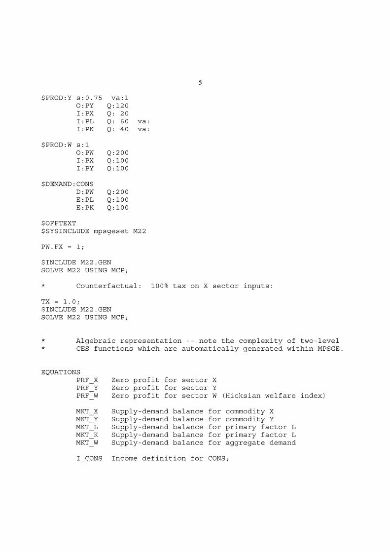
Model M22

We begin with model M22, which introduces intermediate goods, and a simple CES

nesting notation that permits the modeler to specify different elasticities of substitution between

different groups of inputs.

This model is shown below. X and Y sectors each use the other sector’s output as an

input, so that each sector has three inputs. With three inputs, there may be different elasticities of

substitution between different pairs of these inputs. Consider the production block for the Y

sector.

$PROD:Y s:0.75 va:1 O:PY Q:120 I:PX Q: 20 I:PL Q: 60 va: I:PK Q: 40 va:

This specifies a two-level nesting structure. Labor and capital are combined in the both

nest with an elasticity of substitution of 1 (va:1). We use VA to denote “value added” although

this is not required and just “a” could be used. The important thing is the syntax used to specify

the structure. Think of the inputs denoted with VA as combined to produce a composite input, in

this case termed value added. The top level of the CES function specifies an elasticity of

substitution of 0.75 (s:0.75) between the intermediate input, in this case X, and the value-added

composite of capital and labor. In some models this is specified as equal to zero, indicating that

a fixed amount of the intermediate input is required for each unit of output. A similar structure is

specified for the X sector, and in addition we all for taxes on X sector inputs.

Following the MPS/GE version of the model, we present the code for the MCP version

with all equations written out. This is done for two purposes. First, it again helps you to

understand exactly what MPS/GE is doing with the simple the specification that you have given

3

to it. Second, it should help convince you of the advantages of MPS/GE. Finding and correctly

specifying the correct CES functions for the X and Y sectors is not an easy manner. But you are

not finished there. You also have to correctly apply Shepard’s lemma to find factor demands for

use in the factor-market-clearing equations. While it is very important to understand exactly

what MPS/GE is doing in the background, we hope this will also convince you to let this higher-

level software do the dirty work.

4

$TITLE Model M22: Closed Economy 2X2 with Intermediate Inputs andNesting

$ONTEXT

Production Sectors Consumers Markets | X Y W | CONS ------------------------------------------------------ PX | 120 -20 -100 | PY | -20 120 -100 | PW | 200 | -200 PL | -40 -60 | 100 PK | -60 -40 | 100 ------------------------------------------------------

$OFFTEXT

PARAMETERS TX;

TX = 0;

$ONTEXT$MODEL: M22




$PROD:X s:0.5 va:1 O:PX Q:120 I:PY Q: 20 I:PL Q: 40 va: A:CONS T:TX I:PK Q: 60 va: A:CONS T:TX

5

$PROD:Y s:0.75 va:1 O:PY Q:120 I:PX Q: 20 I:PL Q: 60 va: I:PK Q: 40 va:


$DEMAND:CONS D:PW Q:200 E:PL Q:100 E:PK Q:100

$OFFTEXT$SYSINCLUDE mpsgeset M22

PW.FX = 1;

$INCLUDE M22.GENSOLVE M22 USING MCP;

* Counterfactual: 100% tax on X sector inputs:

TX = 1.0;$INCLUDE M22.GENSOLVE M22 USING MCP;

* Algebraic representation -- note the complexity of two-level * CES functions which are automatically generated within MPSGE.

EQUATIONS PRF_X Zero profit for sector X PRF_Y Zero profit for sector Y PRF_W Zero profit for sector W (Hicksian welfare index)

MKT_X Supply-demand balance for commodity X MKT_Y Supply-demand balance for commodity Y MKT_L Supply-demand balance for primary factor L MKT_K Supply-demand balance for primary factor L MKT_W Supply-demand balance for aggregate demand


6

PRF_X.. 120 * ( 1/6 * PY**(1-0.5) + 5/6 * (PL**0.4 * PK**0.6 * (1+TX))**(1-0.5))**(1/(1-0.5)) =E= 120 * PX;

PRF_Y.. 120 * ( 1/6 * PX**(1-0.75) + 5/6 * (PL**0.6 * PK**0.4)** (1-0.75) )**(1/(1-0.75)) =E= 120 * PY;

PRF_W.. 200 * PX**0.5 * PY**0.5 =E= 200 * PW;

MKT_X.. 120 * X =E= 100 * W * PX**0.5 * PY**0.5 / PX + 20*Y*(PY/PX)**0.75;

MKT_Y.. 120 * Y =E= 100 * W * PX**0.5 * PY**0.5 / PY + 20*X*(PX/PY)**0.5;


MKT_L.. 100 =E= 40 * X * (PX/((1+TX)*PL**0.4*PK**0.6))**0.5 * PL**0.4 * PK**0.6 / PL + 60 * Y * (PY/(PL**0.6 * PK**0.4))**0.75 * PL**0.6 * PK**0.4 / PL;

MKT_K.. 100 =E= 60 * X * (PX/((1+TX)*PL**0.4*PK**0.6))**0.5 * PL**0.4 * PK**0.6 / PK + 40 * Y * (PY/(PL**0.6 * PK**0.4))**0.75 * PL**0.6 * PK**0.4 / PK;

I_CONS.. CONS =E= 100*PL + 100*PK + TX * 100 * X * PL**0.4*PK**0.6 * (PX/((1+TX)*PL**0.4*PK**0.6))**0.5;

MODEL ALGEBRAIC /PRF_X.X, PRF_Y.Y, PRF_W.W, MKT_X.PX, MKT_Y.PY,MKT_L.PL, MKT_K.PK, MKT_W.PW, I_CONS.CONS /;

* Check the benchmark:

X.L=1; Y.L=1; W.L=1; PX.L=1; PY.L=1; PK.L=1; PW.L=1; CONS.L=200;

TX = 0; SOLVE ALGEBRAIC USING MCP;

* Solve the same counterfactual:

TX = 1; SOLVE ALGEBRAIC USING MCP;

7

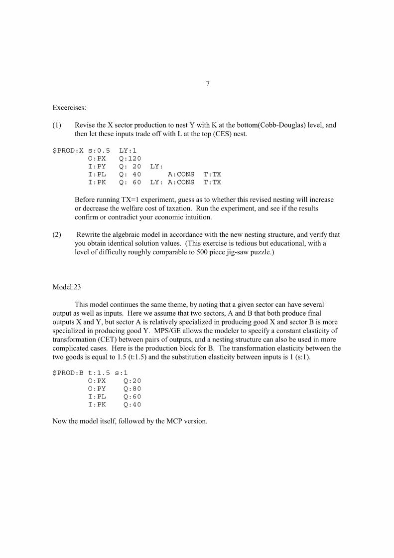
Excercises:

(1) Revise the X sector production to nest Y with K at the bottom(Cobb-Douglas) level, and

then let these inputs trade off with L at the top (CES) nest.

$PROD:X s:0.5 LY:1 O:PX Q:120 I:PY Q: 20 LY: I:PL Q: 40 A:CONS T:TX I:PK Q: 60 LY: A:CONS T:TX

Before running TX=1 experiment, guess as to whether this revised nesting will increase

or decrease the welfare cost of taxation. Run the experiment, and see if the results

confirm or contradict your economic intuition.

(2) Rewrite the algebraic model in accordance with the new nesting structure, and verify that

you obtain identical solution values. (This exercise is tedious but educational, with a

level of difficulty roughly comparable to 500 piece jig-saw puzzle.)

Model 23

This model continues the same theme, by noting that a given sector can have several

output as well as inputs. Here we assume that two sectors, A and B that both produce final

outputs X and Y, but sector A is relatively specialized in producing good X and sector B is more

specialized in producing good Y. MPS/GE allows the modeler to specify a constant elasticity of

transformation (CET) between pairs of outputs, and a nesting structure can also be used in more

complicated cases. Here is the production block for B. The transformation elasticity between the

two goods is equal to 1.5 (t:1.5) and the substitution elasticity between inputs is 1 (s:1).

$PROD:B t:1.5 s:1 O:PX Q:20 O:PY Q:80 I:PL Q:60 I:PK Q:40

Now the model itself, followed by the MCP version.

8

$TITLE Model M23: Closed Economy 2x2 with Joint Production

$ONTEXT

Production Sectors Consumers Markets | A B W | CONS ------------------------------------------------------ PX | 80 20 -100 | PY | 20 80 -100 | PW | 200 | -200 PL | -40 -60 | 100 PK | -60 -40 | 100 ------------------------------------------------------

$OFFTEXT

PARAMETERS TA;

TA = 0;

$ONTEXT

$MODEL: M23

$SECTORS: A ! Activity level for sector A (80:20 for X:Y) B ! Activity level for sector B (20:80 for X:Y) W ! Activity level for sector W (Hicksian welfare index)



$PROD:A t:2.0 s:1 O:PX Q:80 O:PY Q:20 I:PL Q:40 A:CONS T:TA I:PK Q:60 A:CONS T:TA

$PROD:B t:1.5 s:1 O:PX Q:20

9

O:PY Q:80 I:PL Q:60 I:PK Q:40




PW.FX = 1;



TA = 0.10;$INCLUDE M23.GENSOLVE M23 USING MCP;


TA = 1.00;$INCLUDE M23.GENSOLVE M23 USING MCP;

* now the mcp version, which again shows you the simplifying features* of MPS/GE

EQUATIONS PRF_A Zero profit for sector X PRF_B Zero profit for sector Y PRF_W Zero profit for sector W (Hicksian welfare index)

MKT_X Supply-demand balance for commodity X MKT_Y Supply-demand balance for commodity Y MKT_L Supply-demand balance for primary factor L MKT_K Supply-demand balance for primary factor

10

MKT_W Supply-demand balance for aggregate demand


* Write the profit constraints as inequalities -- the tax* can cause sector A to shut down completely:

PRF_A.. 100 * PL**0.4 * PK**0.6 * (1+TA) =G= 100 * (0.8 * PX**(1+2.0) + 0.2 * PY**(1+2.0))**(1/(1+2.0));

PRF_B.. 100 * PL**0.6 * PK**0.4 =G= 100 * (0.2 * PX**(1+1.5) + 0.8 * PY**(1+1.5))**(1/(1+1.5));

PRF_W.. 200 * PX**0.5 * PY**0.5 =E= 200 * PW;

MKT_X.. 80 * A *(PX/(0.8*PX**(1+2.0)+0.2*PY**(1+2.0))**(1/(1+2.0)))**2 + 20 * B *(PX/(0.2*PX**(1+1.5)+0.8*PY**(1+1.5))**(1/(1+1.5)))**1.5 =E= 100 * W * PX**0.5 * PY**0.5 / PX;

MKT_Y.. 20 * A *(PY/(0.8*PX**(1+2.0)+0.2*PY**(1+2.0))**(1/(1+2.0)))**2.0 + 80 * B *(PY/(0.2*PX**(1+1.5)+0.8*PY**(1+1.5))**(1/(1+1.5)))**1.5 =E= 100 * W * PX**0.5 * PY**0.5 / PY;


MKT_L.. 100 =E= 40 * A * PL**0.4 * PK**0.6 / PL + 60 * B * PL**0.6 * PK**0.4 / PL;

MKT_K.. 100 =E= 60 * A * PL**0.4 * PK**0.6 / PK + 40 * B * PL**0.6 * PK**0.4 / PK;

I_CONS.. CONS =E= 100*PL + 100*PK + TA*100*A*PL**0.4*PK**0.6;

MODEL ALGEBRAIC /PRF_A.A, PRF_B.B, PRF_W.W, MKT_X.PX, MKT_Y.PY,MKT_L.PL, MKT_K.PK, MKT_W.PW, I_CONS.CONS /;

* Check the benchmark:

A.L=1; B.L=1; W.L=1; PX.L=1; PY.L=1; PK.L=1; PW.L=1; CONS.L=200;

TA = 0; SOLVE ALGEBRAIC USING MCP;

* Solve the same counterfactuals:

TA = 0.10;SOLVE ALGEBRAIC USING MCP;

11

TA = 1.00;SOLVE ALGEBRAIC USING MCP;

Exercises:

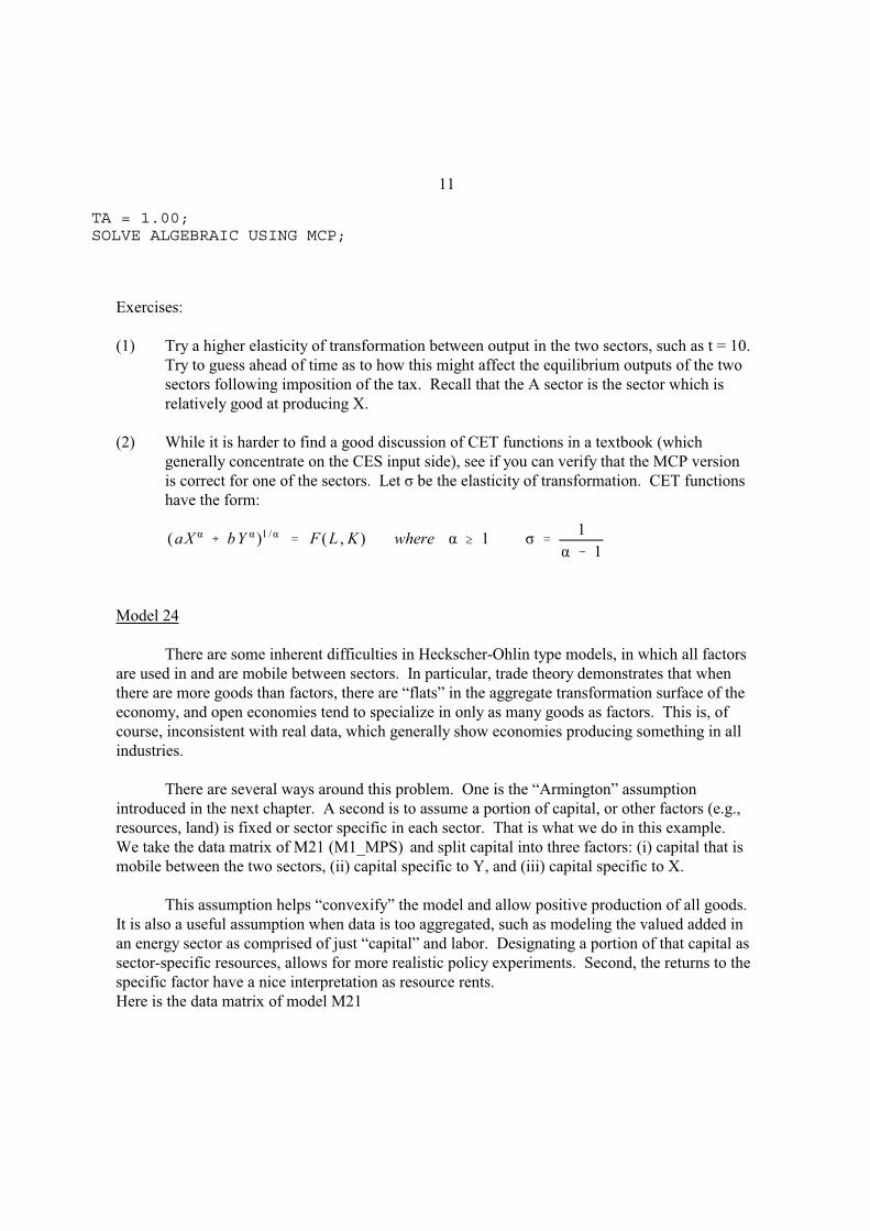
(1) Try a higher elasticity of transformation between output in the two sectors, such as t = 10.

Try to guess ahead of time as to how this might affect the equilibrium outputs of the two

sectors following imposition of the tax. Recall that the A sector is the sector which is

relatively good at producing X.

(2) While it is harder to find a good discussion of CET functions in a textbook (which

generally concentrate on the CES input side), see if you can verify that the MCP version

is correct for one of the sectors. Let be the elasticity of transformation. CET functions

have the form:

(aX bY )1/ F (L , K ) where 11

1

Model 24

There are some inherent difficulties in Heckscher-Ohlin type models, in which all factors

are used in and are mobile between sectors. In particular, trade theory demonstrates that when

there are more goods than factors, there are “flats” in the aggregate transformation surface of the

economy, and open economies tend to specialize in only as many goods as factors. This is, of

course, inconsistent with real data, which generally show economies producing something in all

industries.

There are several ways around this problem. One is the “Armington” assumption

introduced in the next chapter. A second is to assume a portion of capital, or other factors (e.g.,

resources, land) is fixed or sector specific in each sector. That is what we do in this example.

We take the data matrix of M21 (M1_MPS) and split capital into three factors: (i) capital that is

mobile between the two sectors, (ii) capital specific to Y, and (iii) capital specific to X.

This assumption helps “convexify” the model and allow positive production of all goods.

It is also a useful assumption when data is too aggregated, such as modeling the valued added in

an energy sector as comprised of just “capital” and labor. Designating a portion of that capital as

sector-specific resources, allows for more realistic policy experiments. Second, the returns to the

specific factor have a nice interpretation as resource rents.

Here is the data matrix of model M21

12


Now designate part of the capital in each sector as fixed in that sector, creating a four-factor

model.

Production Sectors Consumers Markets | X Y W | CONS ------------------------------------------------------ PX | 100 -100 | PY | 100 -100 | PW | 200 | -200 PL | -25 -75 | 100 PK | -50 -15 | 65 PKX | -25 | 25 PKY | -10 | 10 ------------------------------------------------------

Exercise:

As an exercise after examining this model, try to guess how the introduction of the specific

factors affects the responsiveness (elasticity) of X and Y outputs to the 100% tax. Run the model

and compare it to the 50% X-sector tax results in model M21 (M1_MPS).

13

$TITLE Model M24: Closed Economy 2x2 with Specific Factors

$ONTEXT

Here is the initial data matrix for example M21 (also M1_MPS). As notedin the text description, it is technically useful to interpret a portionof capital in each sector as sector specific. Or it can in fact be a separate factor such as land or resources.


Designate part of the capital in each sector as fixed in that sector

Production Sectors Consumers Markets | X Y W | CONS ------------------------------------------------------ PX | 100 -100 | PY | 100 -100 | PW | 200 | -200 PL | -25 -75 | 100 PK | -50 -15 | 65 PKX | -25 | 25 PKY | -10 | 10 ------------------------------------------------------

$OFFTEXT

PARAMETERS TX;

TX = 0;

$ONTEXT$MODEL:M24


14

$COMMODITIES: PW ! Price index for welfare (expenditure function) PX ! Price index for commodity X PY ! Price index for commodity Y PL ! Price index for primary factor L PK ! Price index for (mobile) capital PKX ! Price index for sector-specific input for sector X PKY ! Price index for sector-specific input for sector Y


$PROD:X s:1 O:PX Q:100 I:PL Q: 25 A:CONS T:TX I:PK Q: 50 A:CONS T:TX I:PKX Q: 25 A:CONS T:TX

$PROD:Y s:1 O:PY Q:100 I:PL Q: 75 I:PK Q: 15 I:PKY Q: 10


$DEMAND:CONS D:PW Q:200 E:PL Q:100 E:PK Q: 65 E:PKX Q: 25 E:PKY Q: 10



* Solve a counterfactual:


15

Model 25

As noted in chapter one, an attractive and powerful feature of MPS/GE is that it solves

complementarity problems in which some production activities can be slack for some values of

parameters and active for others. This allows researchers to consider a much wider set of

problems that is allowed using software which can only solve systems of equations.

Model 25 presents a simple example, motivated by tax evasion activities. There is a third

sector, Z, which also produces good X but it is 10% less efficient (10% more costly) than the X

activity itself. So initially, Z does not operate. But when a tax of 25% is imposed on X, this

activity goes slack and Z begins to operate. We could think of Z as a tax evasion or “informal”

activity that is less efficient but can successfully avoid the tax.

Exercise:

As a second counterfactual, we impose the tax but do not let the Z sector operate by imposing the

restriction Z.FX = 0;. Compare the results of this run to the first counterfactual in which Z is

allowed to operate. Can you interpret the welfare results? Hint: while the tax is distortionary,

the switch to the inefficient activity uses real resources to avoid the tax.

Now raise the tax to 100%. Does this result that tax evasion (the switch to Z) is welfare

worsening still hold?

16

$TITLE Model M25: Closed 2x2 Economy with an Unprofitable Activity

$ONTEXT


Activity Z is unprofitable at initial equilibrium prices. It istherefore not operated, and we cannot infer its technical propertiesfrom the benchmark social accounting data. We assume that Z is 10% less efficient than X.

$OFFTEXT

PARAMETERS TX;

TX = 0;

$ONTEXT$MODEL:M25

$SECTORS: X ! Activity level for sector X Y ! Activity level for sector Y W ! Activity level for sector W (Hicksian welfare index) Z ! Alternative activity for producing X.



$PROD:X s:1 O:PX Q:100 I:PL Q: 40 A:CONS T:TX

17

I:PK Q: 60 A:CONS T:TX

$PROD:Y s:1 O:PY Q:100 I:PL Q: 60 I:PK Q: 40

$PROD:Z s:1 O:PX Q:100 I:PL Q: 44 I:PK Q: 66




PW.FX = 1;

Z.L = 0;

$INCLUDE M25.GENSOLVE M25 USINCP MCP;

* Let’s levy a high on sector X and see what happens:


* What is the effect of the tax if Z could not be used?

Z.FX = 0;


18

Model M26

Often general-equilibrium models used in international trade assume that factors of

production, especially labor, are in fixed and inelastic supply. But designing tax, welfare, and

education systems, endogenizing labor supply is a crucial part of the story. Model M26

endogenizes labor supply, allowing labor to chose between leisure and labor supply with leisure

entering into the workers utility function.

This requires the modeler to specify an endowment of labor or time, something which is

not in itself directly observable. Only the portion actually supplied to the market is observable.

The modeler also need to specify an elasticity of substitution between leisure and consumption

goods, which will in turn imply an elasticity of labor supply.

We cannot do much theoretical analysis here, but do suggest that students interested in

these questions work with a simple CES function with one good and leisure in order to

understand the basic mircoeconomics of labor supply. For a Cobb-Douglas function with an

elasticity of substitution equal to one between consumption and leisure, labor supply is

completely inelastic with respect to the wage rate. When the elasticity of substitution is greater

than one, an increase in the wage rate will mean an increase in labor supply, and an elasticity of

substitution less than one will mean that labor supply is “backward bending”, falling with an

increase in the wage rate.

In our formulation, we introduce an additional activity T, which transforms leisure (price

PL) into labor supplied (price PLS). Strictly speaking this is not necessary, the consumer’s

endowment of labor could just be supplied to both production and the welfare generating activity

W. But adding activities is often useful. The solution will report the activity level of T which

allows us to directly check the change in labor supply, and any tax on labor can be specified here

just once rather than in each sector that uses labor. Here is the production block for T.

$PROD:T O:PLS Q:100 I:PL Q:100 A:CONS T:TL

The production block for W specifies a nesting structure in which goods have an elasticity of

substitution of 1 between them in a lower nest, and goods and leisure have an elasticity of

substitution between them of 0.5.

$PROD:W s:0.5 cons:1 O:PW Q:300 I:PX Q:100 cons: I:PY Q:100 cons: I:PL Q:100

The consumer is assumed to be endowed with 200 units of labor/leisure (found in the DEMAND

19

block), of which 100 units are supplied to the labor market initially.

$TITLE Model M26: 2x2 Economy with Labor-Leisure Choice

$ONTEXT

Activity T transforms leisure into labor supply:

Production Sectors Consumers Markets | A B W T | CONS --------------------------------------------------------- PX | 80 20 -100 | PY | 20 80 -100 | PW | 300 | -300 PLS | -40 -60 100 | PL | -100 -100 | 200 PK | -60 -40 | 100 ---------------------------------------------------------

$OFFTEXT

PARAMETERS TL WELFARE REALCONS;

TL = 0;

$ONTEXT$MODEL:M26

$SECTORS: X ! Activity level for sector X Y ! Activity level for sector Y T ! Labor supply W ! Activity level for sector W (Hicksian welfare index)

$COMMODITIES: PX ! Price index for commodity X PY ! Price index for commodity Y PL ! Price index for leisure PLS ! Price index for labor supply (factor L input) PK ! Price index for primary factor K PW ! Price index for welfare (expenditure function)


20

$PROD:X s:1 O:PX Q:100 I:PLS Q: 40 I:PK Q: 60

$PROD:Y s:1 O:PY Q:100 I:PLS Q: 60 I:PK Q: 40

$PROD:T O:PLS Q:100 I:PL Q:100 A:CONS T:TL

$PROD:W s:0.5 cons:1 O:PW Q:300 I:PX Q:100 cons: I:PY Q:100 cons: I:PL Q:100



PW.FX = 1;


WELFARE = W.L;REALCONS = (PX.L*X.L*100 + PY.L*Y.L*100)/(PX.L**0.5*PY.L**0.5*200);DISPLAY WELFARE, REALCONS;

* Solve a counter-factual, tax labor supply at 25%

TL = 0.5;$INCLUDE M26.GENSOLVE M26 USING MCP;

WELFARE = W.L;REALCONS = (PX.L*X.L*100 + PY.L*Y.L*100)/(PX.L**0.5*PY.L**0.5*200);DISPLAY WELFARE, REALCONS;

21

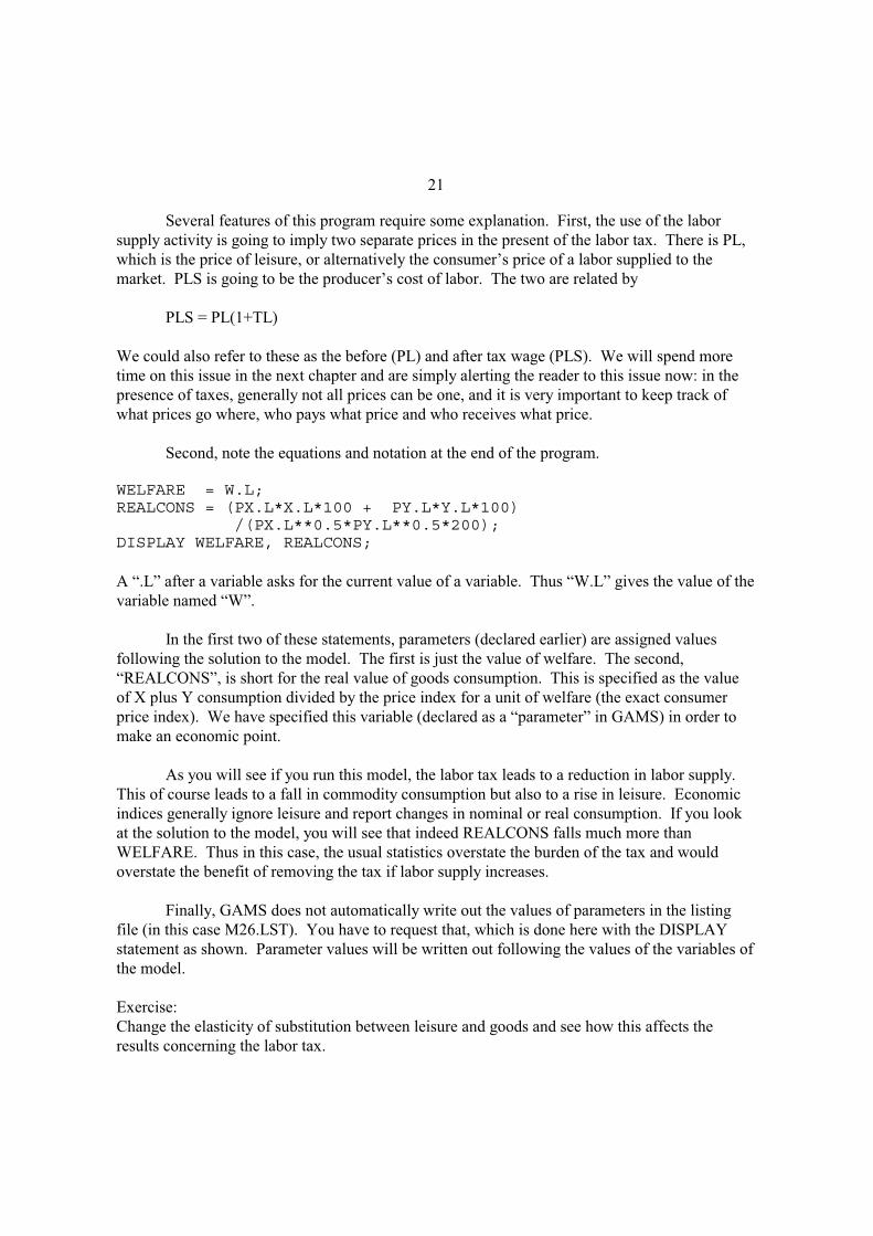
Several features of this program require some explanation. First, the use of the labor

supply activity is going to imply two separate prices in the present of the labor tax. There is PL,

which is the price of leisure, or alternatively the consumer’s price of a labor supplied to the

market. PLS is going to be the producer’s cost of labor. The two are related by

PLS = PL(1+TL)

We could also refer to these as the before (PL) and after tax wage (PLS). We will spend more

time on this issue in the next chapter and are simply alerting the reader to this issue now: in the

presence of taxes, generally not all prices can be one, and it is very important to keep track of

what prices go where, who pays what price and who receives what price.

Second, note the equations and notation at the end of the program.

WELFARE = W.L;REALCONS = (PX.L*X.L*100 + PY.L*Y.L*100) /(PX.L**0.5*PY.L**0.5*200);DISPLAY WELFARE, REALCONS;

A “.L” after a variable asks for the current value of a variable. Thus “W.L” gives the value of the

variable named “W”.

In the first two of these statements, parameters (declared earlier) are assigned values

following the solution to the model. The first is just the value of welfare. The second,

“REALCONS”, is short for the real value of goods consumption. This is specified as the value

of X plus Y consumption divided by the price index for a unit of welfare (the exact consumer

price index). We have specified this variable (declared as a “parameter” in GAMS) in order to

make an economic point.

As you will see if you run this model, the labor tax leads to a reduction in labor supply.

This of course leads to a fall in commodity consumption but also to a rise in leisure. Economic

indices generally ignore leisure and report changes in nominal or real consumption. If you look

at the solution to the model, you will see that indeed REALCONS falls much more than

WELFARE. Thus in this case, the usual statistics overstate the burden of the tax and would

overstate the benefit of removing the tax if labor supply increases.

Finally, GAMS does not automatically write out the values of parameters in the listing

file (in this case M26.LST). You have to request that, which is done here with the DISPLAY

statement as shown. Parameter values will be written out following the values of the variables of

the model.

Exercise:

Change the elasticity of substitution between leisure and goods and see how this affects the

results concerning the labor tax.

22

Model M27

This is a model which may be of interest to development and public finance economists.

It assumes that there are two labor markets, a “formal” and an “informal” market. Governments

are able to collect taxes on the former but not on the latter. The representative household can

choose how much labor to supply to each market. For simplicity, we assume that there is no

labor-leisure decision, and that all labor is supplied to one of the two markets, but that can be

very easily added and indeed we will suggest that as an exercise at the end.

There are many ways of doing this. We first of all use an activity denoted LS which takes

household labor and produces two outputs, formal and informal labor (prices PLSF and PLSI)

according to a CET transformation function with an elasticity 5.0. Think of this as a household

technology embodying the fact that the two types of labor are not perfect substitutes in supply.

For example, this might be a crude simplification of the fact that the representative household is

actual many households (or household locations) some of whom are better at supplying formal

labor and vice versa. Concentrating supply in either market leads to something like “diminishing

returns”, a concave transformation frontier between the two types of labor.

In addition, the two types of labor can be imperfect substitutes on the production side.

That is what we assume here. Only formal labor is used in the X sector, while both formal and

(mostly) informal labor are used in the Y sector. The two types of labor are in a lower level nest

with an elasticity of substitution of 3.

The formal and informal labor supplies could go directly into production, but the listing

file will not directly tell us how much of each type is produced by activity LS. Thus we use two

“dummy” activities LF and LI which take a unit of formal labor (LF) or informal labor (LI) and

just turn each unit into a unit of the same thing with a different commodity name (PLF and PLI)

which are the actual inputs into production. This is just a trip so that the listing file will tell us

how much of each type of labor is supplied, the activity levels of LF and LI respectively. In

addition, this trick is convenient in multi-sector models because the tax on formal labor need

only be specified once, in the LF activity, and not in every production block using formal labor.

Here is the program. You will see from the listing file that the tax on formal labor supply

leads to a large shift of household supply toward informal labor and that there is a large shift in

output toward Y, the sector using informal labor.

23

$TITLE Model M27: 2x2 Economy with Formal/Informal Labor Supply

$ONTEXT

Activity LS transforms leisure into formal and informal labor supplies.LF and LI are "dummy" activities used to keep track of how much laboris supplied to each market.

Production Sectors ConsumersMarkets | X Y W LF LI LS | CONS------------------------------------------------------------------- PX | 100 -100 | PY | 100 -100 | PW | 200 | -200 PLF | -40 -10 50 | PLI | -50 50 | PLSF | -50 50 | PLSI | -50 50 | PL | -100 | 100 PK | -60 -40 | 100 ----------------------------------------------------------------

$OFFTEXT

PARAMETERS TL;

TL = 0;

$ONTEXT$MODEL:M27

$SECTORS: X ! Activity level for sector X Y ! Activity level for sector Y LS ! Activity level for household labor supply LF ! Activity for formal labor supply LI ! Activity for informal labor supply W ! Activity level for sector W (Hicksian welfare index)

$COMMODITIES: PX ! Price index for commodity X PY ! Price index for commodity Y PL ! Price index for labor PLSF ! Price index for formal labor supplied to market PLSI ! Price index for informal labor supply to market PLF ! Price index for formal labor supplied to firms

24

PLI ! Price index for informal labor supplied to firms PK ! Price index for primary factor K PW ! Price index for welfare (expenditure function)


$PROD:X s:1 O:PX Q:100 I:PLF Q: 40 I:PK Q: 60

$PROD:Y s:1 a:3 O:PY Q:100 I:PLF Q: 10 a: I:PLI Q: 50 a: I:PK Q: 40

$PROD:LS t:5.0 O:PLSF Q: 50 O:PLSI Q: 50 I:PL Q:100

$PROD:LF O:PLF Q: 50 I:PLSF Q: 50 A:CONS T:TL

$PROD:LI O:PLI Q: 50 I:PLSI Q: 50

$PROD:W s:1.0 O:PW Q:200 I:PX Q:100 I:PY Q:100



PW.FX = 1;


25

* Solve a counter-factual, tax formal labor supply at 50%

TL = 0.5;$INCLUDE M27.GENSOLVE M27 USING MCP;

Model M28

A great many questions of interest to trade and public finance economists involve issues

of distribution rather than or in addition to issues of aggregate welfare. Households (or

“consumers” in MPS/GE) may differ in their preferences and more importantly in their sources

of income (or their factor endowments). For both reasons, different taxes and other government

policies affect different households in different ways. In addition to creating deadweight losses

or aggregate benefits, tax change can also significantly redistribute income among households.

Adding multiple household types is a straightforward extension of our earlier models. In

model M28, we allow for two households. Household A is relatively well endowed with labor,

and also has a preference for good Y, which is the labor-intensive good. Household B is

relatively well endowed with capital and has a relative preference for the capital intensive good

X.

Our counterfactual experiment is to place a tax on the factor inputs to X, assigning half

the revenue to each consumer. As you will guess, this tax lowers the welfare of household B.

However, the redistribution effect outweighs the overall deadweight loss of the tax for household

A, which is actually better off. This welfare gain is a combination of a redistribution in favor of

capital, and a lowering of the relative consumer price of Y, the good favored by household A.

Note that we chose labor as numeraire in this program, and the consumer price index (PWA,

PWB) will differ for the two households.

Exercises:

(1) You might (correctly) guess that there is no way to redistribute the tax unevenly and make

both households worse off. That would violate the first theorem of welfare economics.

Try some alternative distributions to check on this. You will need to specify two

different tax parameters, but they should continue to sum to 0.5 = 2*0.25.

(1) Recalibrate the data so that the households have the same preferences. Running the

experiment gives then a welfare effect due only to the change in factor prices following

the imposition of the tax.

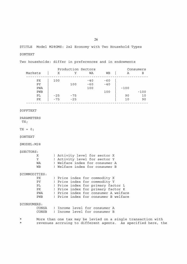
26

$TITLE Model M28GMS: 2x2 Economy with Two Household Types

$ONTEXT

Two households: differ in preferences and in endowments

Production Sectors Consumers Markets | X Y WA WB | A B ---------------------------------------------------------- PX | 100 -40 -60 | PY | 100 -60 -40 | PWA | 100 | -100 PWB | 100 | -100 PL | -25 -75 | 90 10 PK | -75 -25 | 10 90 ----------------------------------------------------------

$OFFTEXT

PARAMETERS TX;

TX = 0;

$ONTEXT

$MODEL:M28

$SECTORS: X ! Activity level for sector X Y ! Activity level for sector Y WA ! Welfare index for consumer A WB ! Welfare index for consumer B

$COMMODITIES: PX ! Price index for commodity X PY ! Price index for commodity Y PL ! Price index for primary factor L PK ! Price index for primary factor K PWA ! Price index for consumer A welfare PWB ! Price index for consumer B welfare

$CONSUMERS: CONSA ! Income level for consumer A CONSB ! Income level for consumer B

* More than one tax may be levied on a single transaction with* revenues accruing to different agents. As specified here, the

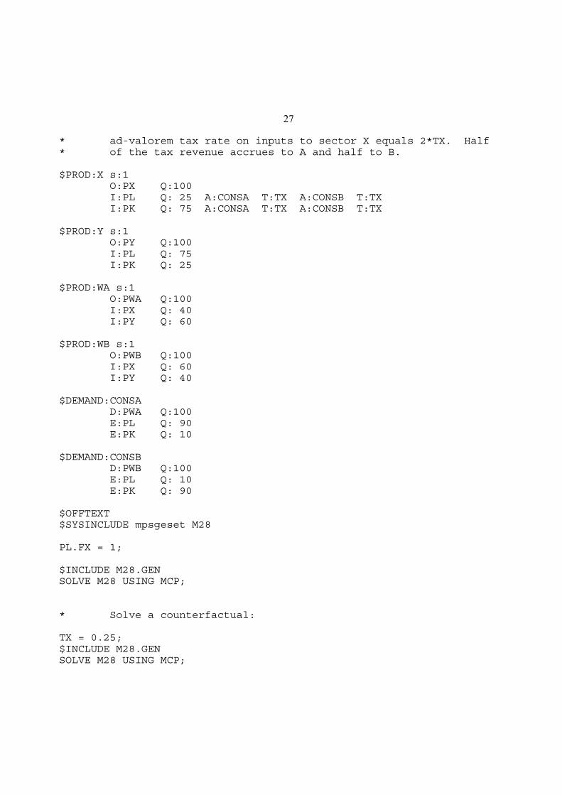
27

* ad-valorem tax rate on inputs to sector X equals 2*TX. Half* of the tax revenue accrues to A and half to B.

$PROD:X s:1 O:PX Q:100 I:PL Q: 25 A:CONSA T:TX A:CONSB T:TX I:PK Q: 75 A:CONSA T:TX A:CONSB T:TX


$PROD:WA s:1 O:PWA Q:100 I:PX Q: 40 I:PY Q: 60

$PROD:WB s:1 O:PWB Q:100 I:PX Q: 60 I:PY Q: 40

$DEMAND:CONSA D:PWA Q:100 E:PL Q: 90 E:PK Q: 10

$DEMAND:CONSB D:PWB Q:100 E:PL Q: 10 E:PK Q: 90


PL.FX = 1;


* Solve a counterfactual:


28

Model 29

No budget study we are aware of has ever suggested that consumer preferences are

homogeneous. Households tend to spend a much higher proportion of their income on food at

low incomes, for example, than at high incomes. Part of the reason that trade economists and

applied general-equilibrium modelers are so fond of homogenous functions is that they are

technically much easier to handle than non-homogeneous functions. As we noted earlier, any

constant-returns CES function can be completely specified by a single vector of values of inputs

and output quantities, and the relative prices of inputs at that point.

One alternative formulation is know as the Stone-Geary utility function, which in turn

gives rise to the linear expenditure system (LES) of demand equations, the latter being popular in

budget studies. The Stone-Geary utility function is just a Cobb-Douglas function with the origin

displaced from zero. These displacements, if positive, are typically called “minimum

consumption requirements”, meaning that the consumer gets no positive utility until these needs

are met. Consider a simple case in which there is a minimum consumption requirement in X but

not in Y. The minimum X consumption is denoted X*. The utility function is

U (X X ) Y 1

If we maximized this subject to the usual budget constraint with income I, the demand functions

for X and Y would be:

X X( I p

xX )

px

Y(1 ) ( I p

xX )

py

pxX p

yY I

The first equation is rather intuitive in words. It says that you first purchase the minimum

consumption requirements, and then you spend a constant fraction ( ) of remaining income net

of the minimum requirements on X. Further algebra would give us the budget share spent on X

and the income elasticity of demand for X.

pxX

I

I (1 )pxX

I

I

X

dX

dI

I

I (1 )pxX

The budget share spent on X falls with increases in income, asymptotically approaching as

income rises. The income elasticity of demand rises with income, asymptotically approaching 1.

Suppose that we want to calibrate our initial data to the assumption that the income

elasticity of demand for X is initially equal to 0.75. If we solve the share equation (equal to 0.5)

in the data and the income-elasticity equation (equal to 0.75 by assumption), we get = 3/8.

This will then allow us to solve for X*, which is X* = 40. The trick is then to revise the

29

benchmark data matrix, giving the consumer a negative endowment of X = 40. The utility

(welfare) function W then has an input of 60 units of X (100 minus the minimum consumption

requirement) and 100 units of Y. At prices of 1 for each good, MPS/GE will then calibrate the

Cobb-Douglas utility function with an = 3/8 (60/160).

The counterfactual experiment in this model is to double the consumers endowment.

Note from the results that there is a shift in consumption toward Y, the high income-elasticity

good. Of course, the change in X and Y consumption cannot be directly interpreted as income

elasticities of demand, since prices will change in general equilibrium. The price of Y will rise

relative to X, and the price of the factor used intensively in Y will rise relative to the price of the

other factor.

One final word of caution about this model and the use of Stone-Geary. Welfare changes

have to be interpreted carefully, because utility is not linear (homogenous of degree 1) in income

at constant prices. As you will see from the results of this simulation, utility (W) more than

doubles as we double the endowment. Note by way of intuition that if income as so low that the

consumer could just barely buy the minimum consumption requirement, then utility would be

zero. Also, we should note that if income is too small to even buy X* (in general equilibrium,

the endowment is insufficient to produce X*), the solver will crash and not compute a solution.

These difficulties are troubling, but we are sure that good policy must consider the fact that really

poor people consume very different bundles of goods than rich people, and this has probably

more to do with non-homogeneity than them having homogeneous but different preferences.

30

$TITLE Model M29: Closed 2x2 Economy -- Stone Geary (LES) Preferences

$ONTEXT

The observed data is:


But calibrated to the model as:

Production Sectors Consumers Markets | X Y W | CONS ------------------------------------------------------ PX | 100 -60 | -40 PY | 100 -100 | PW | 160 | -160 PL | -40 -60 | 100 PK | -60 -40 | 100 ------------------------------------------------------

$OFFTEXT

PARAMETERS ENDOW;

ENDOW = 1;

$ONTEXT

$MODEL:M29


31



$PROD:X s:1 O:PX Q:100 I:PL Q: 40 I:PK Q: 60


$PROD:W s:1 O:PW Q:160 I:PX Q: 60 I:PY Q:100

$DEMAND:CONS D:PW Q:160 E:PL Q:(100*ENDOW) E:PK Q:(100*ENDOW) E:PX Q:-40


PW.FX = 1;


* Counterfactual: double the factor endowment.

ENDOW = 2;


1

Chapter 3

Taxes, Tax Reform, Public Goods, and Steady-State Models

Introduces Auxiliary Variables, Constraints, and Rationing

In this chapter, we will begin with a simple problem in which there are taxes in the initial

benchmark data, to illustrate how to calibrate a model with existing taxes. Then we will consider

labor taxes with endogenous labor supply. These models will make the point that some taxes are

less distortionary than others. However, replacing one tax with another rarely yields the same

revenue in general equilibrium. Thus our third example will show how to model tax reforms that

yield the government the same amount of revenue, referred to as “equal-yield tax reform”. In

doing so, we will introduce a major feature of MPS/GE, the auxiliary variable and the constraint

equation. The new tax rate will be an endogenous tax, whose value is set in general equilibrium

by the revenue constraint.

Next, we will introduce a public good, and show how that is modeled. Then we will set

the tax rate to finance this public good endogenously according to the Samuelson rule for pure

public goods. This will also involve the use of an endogenous tax rate, an auxiliary variable, and

a constraint equation. But it will also involve the introduction of another new feature, the

rationing constraint.

Finally, we will end this chapter with two other extensions that are valuable for policy

analysis. First, we will consider taxes and classical unemployment. Second, we will consider an

endogenous capital stock that adjusts according to a steady-state rule. Comparative statics

experiments are then in fact comparative steady-state experiments, showing the general-

equilibrium change in all variables after the capital stock has adjusted to its new general-

equilibrium level.

The models in this chapter are as follows:

M31S.GMS closed economy 2x2 with taxes in the benchmark

M32S.GMS closed economy 2x2 with labor supply and labor tax

M33S.GMS closed economy 2x2, equal yield tax reform

M34S.GMS closed economy 2x2 with a public good

M35.GMS closed economy 2x2, public good using samuelson rule

M36.GMS closed economy 2x2, taxes and classical unemployment

2

M37.GMS closed economy 2x2, steady-state capital stock

Model M31

Our first model is similar to the models of the previous chapter, but a positive tax and tax

revenue are present in the benchmark data. The first task of the modeler is again to construct a

micro-consistent data set, and the format we introduced in chapter 1 (dubbed the micro-

consistency matrix) is a nice way to do this and at the same time set up the data for building the

model. Remember that entries into this matrix are values. Row sums equal to zero indicate

market clearing and column sums equal to zero indicate product exhaustion (zero profits) or

consumer income balance.

Under this convention, each tax should be added as a row to the matrix. Taxes are

negative entries in a column indicating payments by a sector. There is a corresponding positive

entry somewhere. In the present case, the tax is simply redistributed lump sum to the consumer,

so the consumer gets a positive entry of the tax revenue. A zero row sum for the tax indicates

that all tax receipts must be paid to someone. Here is our matrix:


Markets | X Y W | CONS ------------------------------------------------------ PX | 100 -100 | PY | 100 -100 | PW | 200 | -200 PL | -20 -60 | 80 PK | -60 -40 | 100 TAX | -20 0 | 20 ------------------------------------------------------

The data indicate that the X sector receives 100 units of revenue, of which 20 is paid in

taxes. This 20 is received as part of the consumer’s income. Note that these data do not indicate

what type of tax is in place. It could be a tax on X output, on all the inputs, or on just one input.

We are going to interpret this as a tax on the labor input into sector X.

A crucial task for the modeler is to keep track of what prices firms and consumers face. It

is (generally) not possible to calibrate a benchmark equilibrium with all prices equal to one. For

example, if a production input is taxed, then if its consumer price (price received by the

consumer) is chosen to be equal to one, then producer price (price paid by the producer) is

specified as (1 + t). On the other hand, if the producer price is unity, the consumer price is

1/(1+t). We will discuss output taxes shortly.

Given that we interpret the above data as a tax on the labor input into the X sector, the

3

data tell us that the tax rate is 100%. The amount paid by the X sector to labor (20) is equal to

the tax revenue (20). Thus if we set the consumer price of labor to 1 (also the price to the Y

sector), then the price of labor to the X sector must be 2.

When the benchmark price of a production input or output is not equal to unity, it is

necessary to add a reference price field to the production block. The relative prices of inputs fix

the marginal rate of substitution (on inputs, marginal rate of transformation on outputs).

Benchmark reference prices and reference quantities are needed in order to correctly fit

(calibrate) the technology to the data. If these fields are not correctly specified, then a run of the

model will not reproduce the benchmark data as an equilibrium.

Here is the correct specification of the X production block (recall that default prices equal

1 so only prices not equal to 1 must be specified).

$PROD:X s:1 O:PX Q:100 I:PL Q: 20 P:2 A:CONS T:TLX I:PK Q: 60

where TLX (for tax on labor in X) is declared as a parameter elsewhere in the file, in order to

permit changes in TLX as counterfactual experiments.

There are two common mistakes that you need to avoid. First is to leave out the price

field thinking that the assignment of the tax will do that for you. That is incorrect, the P:2 must

appear in the block. The tax itself is not used in the calibration, the Q and P fields are.

Second, the P field must not be specified as P:(1 + TLX). While this would result in the

correct initial calibration, any subsequent change in TLX in a counterfactual would result in a

recalibration of the technology. Assuming that the modeler wants to just change the tax, not the

technology, the P field must have a constant in it. Of course, this constant could itself be a

parameter specified somewhere else in the file (e.g., P:(1 + TLX0)), but it must be constant and

distinct from the changing tax rate.

In some instances, the modeler may of course want to change the technology itself as a

counterfactual. That is fine, but be clear on what it is you want to change.

Finally, we are going to allow for alternative taxes in the model, including a tax on capital

inputs into X (TKX) and a tax on X output (TX). So the production block in the model is written

as follows, where TKX and TX are set to zero initially.

$PROD:X s:1 O:PX Q:100 A:CONS T:TX I:PL Q: 20 P:2 A:CONS T:TLX I:PK Q: 60 A:CONS T:TKX

4

In the first counterfactual, eliminate taxes on X sector inputs and replace with a single tax

on X sector output. We make a guess that the 100% tax on labor might generate revenue roughly

equivalent to a tax of 25% on both inputs: 20 units of revenue is 100% of the benchmark labor

input, or 25% of total benchmark inputs of labor and capital (20 + 60 = 80). Of course, they will

not in fact generate the same revenue as other variables adjust in general equilibrium. Further

discussion of this issue is postponed until model M33.

Now consider a tax on X sector output. It is important to understand that the output tax

rate will be different from the corresponding tax rate on all inputs, because the tax base is

different in the two cases. Let mc denote the marginal cost of production (or producer price) and

p denote the price charged to the consumer. This is how MPS/GE interprets input (ti) versus

output (to) taxes.

Tax on all inputs: p = (1 + ti)mc

Tax on the output: p(1 - to) = mc

Note mc is the tax base for the input tax, and p is the tax base for the output tax. These are not

the same. The output tax that is equivalent to the tax on all inputs is found by:

(1 ti )1

1 to

If ti = TLX = TKX = 0.25 as we have assumed in our first counterfactual, then the equivalent

output tax is given by to = TX = 0.20. Thus in our second counterfactual, we set the input taxes

to zero and the output tax to 0.20.

One more equivalence can be demonstrated with this small model. The final

counterfactual demonstrates that a 20% tax on the output of X is the same as a 25% subsidy to

the production of Y. Let t be the tax on X and s the subsidy to Y. Formally, we have

px(1 t )

py

px

py(1 s )

mcx

mcy

if t 0.20 , s 0.25

Absolute prices may differ depending on the choice of the numeraire, but all quantities and

welfare are the same.

Here is the program.

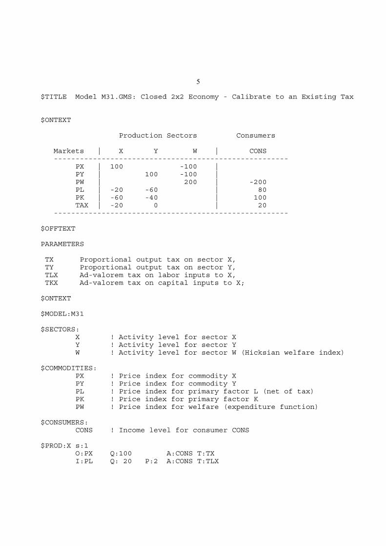
5

$TITLE Model M31.GMS: Closed 2x2 Economy - Calibrate to an Existing Tax

$ONTEXT


Markets | X Y W | CONS ------------------------------------------------------ PX | 100 -100 | PY | 100 -100 | PW | 200 | -200 PL | -20 -60 | 80 PK | -60 -40 | 100 TAX | -20 0 | 20 ------------------------------------------------------

$OFFTEXT

PARAMETERS

TX Proportional output tax on sector X, TY Proportional output tax on sector Y, TLX Ad-valorem tax on labor inputs to X, TKX Ad-valorem tax on capital inputs to X;

$ONTEXT

$MODEL:M31


$COMMODITIES: PX ! Price index for commodity X PY ! Price index for commodity Y PL ! Price index for primary factor L (net of tax) PK ! Price index for primary factor K PW ! Price index for welfare (expenditure function)


$PROD:X s:1 O:PX Q:100 A:CONS T:TX I:PL Q: 20 P:2 A:CONS T:TLX

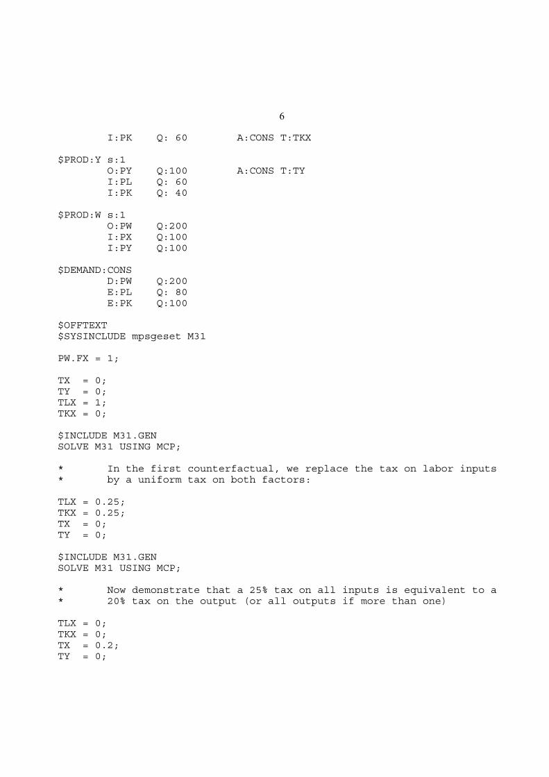
6

I:PK Q: 60 A:CONS T:TKX

$PROD:Y s:1 O:PY Q:100 A:CONS T:TY I:PL Q: 60 I:PK Q: 40


$DEMAND:CONS D:PW Q:200 E:PL Q: 80 E:PK Q:100


PW.FX = 1;

TX = 0;TY = 0;TLX = 1;TKX = 0;


* In the first counterfactual, we replace the tax on labor inputs* by a uniform tax on both factors:

TLX = 0.25;TKX = 0.25;TX = 0;TY = 0;


* Now demonstrate that a 25% tax on all inputs is equivalent to a* 20% tax on the output (or all outputs if more than one)

TLX = 0;TKX = 0;TX = 0.2;TY = 0;

7


* Finally, demonstrate that a 20% tax on the X sector output is * equivalent to a 25% subsidy on Y sector output (assumes that the* funds for the subsidy can be raised lump sum from the consumer!)

TKX = 0;TLX = 0;TX = 0;TY = -0.25;


Exercises:

(1) Verify that the results from all the counterfactuals accord with our theoretical intuition

(2) Set the price field for PL in the PROD:X block in the benchmark equal to one,

deliberately creating an error. Run the model and verify that the first solution does not

reproduce the benchmark.

(3) Deliberately create a second error. Set the price field equal to P:(1 + TLX). Run the

model, and see that this replicates the benchmark, but gives different answers to the

counterfactuals than with P:2.

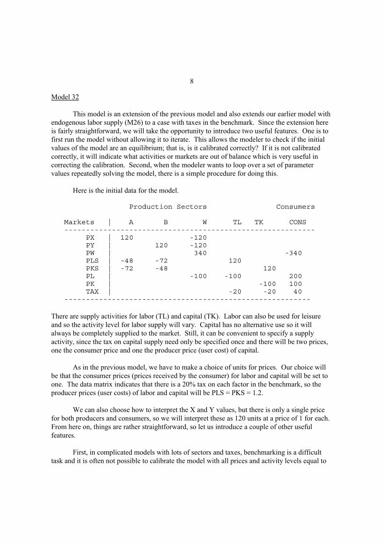
8

Model 32

This model is an extension of the previous model and also extends our earlier model with

endogenous labor supply (M26) to a case with taxes in the benchmark. Since the extension here

is fairly straightforward, we will take the opportunity to introduce two useful features. One is to

first run the model without allowing it to iterate. This allows the modeler to check if the initial

values of the model are an equilibrium; that is, is it calibrated correctly? If it is not calibrated

correctly, it will indicate what activities or markets are out of balance which is very useful in

correcting the calibration. Second, when the modeler wants to loop over a set of parameter

values repeatedly solving the model, there is a simple procedure for doing this.

Here is the initial data for the model.


Markets | A B W TL TK CONS ---------------------------------------------------------- PX | 120 -120 PY | 120 -120 PW | 340 -340 PLS | -48 -72 120 PKS | -72 -48 120 PL | -100 -100 200 PK | -100 100 TAX | -20 -20 40 ---------------------------------------------------------

There are supply activities for labor (TL) and capital (TK). Labor can also be used for leisure

and so the activity level for labor supply will vary. Capital has no alternative use so it will

always be completely supplied to the market. Still, it can be convenient to specify a supply

activity, since the tax on capital supply need only be specified once and there will be two prices,

one the consumer price and one the producer price (user cost) of capital.

As in the previous model, we have to make a choice of units for prices. Our choice will

be that the consumer prices (prices received by the consumer) for labor and capital will be set to

one. The data matrix indicates that there is a 20% tax on each factor in the benchmark, so the

producer prices (user costs) of labor and capital will be PLS = PKS = 1.2.

We can also choose how to interpret the X and Y values, but there is only a single price

for both producers and consumers, so we will interpret these as 120 units at a price of 1 for each.

From here on, things are rather straightforward, so let us introduce a couple of other useful

features.

First, in complicated models with lots of sectors and taxes, benchmarking is a difficult

task and it is often not possible to calibrate the model with all prices and activity levels equal to

9

one. One useful trick for checking the calibration and noting which sectors or markets are out of

balance is to not allow the model to iterate initially. After the MPS/GE model itself, you will see

the notation:

PLS.L =1.2; PKS.L =1.2;

M32.ITERLIM = 0;


M32.ITERLIM = 2000;

First, we set initial values for any activities or prices that we know do not take on the

default values of 1. This is done with the .L suffix on the variable that we used once before.

Note that this does not fix the value of the variable (that is the .FX suffix), it just sets its initial

value.

Next we use a command which tells GAMS that it cannot iterate in attempting to solve

the model (syntax is <model name>.ITERLIM = 0;). Then we use the INCLUDE and SOLVE

statements. Then, in preparation for the next run we set the iteration limit back to a high value.

Suppose that we had set the initial value of PLS.L = 1.0 instead of 1.2. This is what you

will see if you look at the listing file (M32.LST).


---- VAR X . 1.000 +INF -8.440---- VAR Y . 1.000 +INF -12.435---- VAR W . 1.000 +INF .---- VAR TL . 1.000 +INF 20.000---- VAR TK . 1.000 +INF .---- VAR PX . 1.000 +INF .---- VAR PY . 1.000 +INF .---- VAR PL . 1.000 +INF .---- VAR PK . 1.000 +INF .---- VAR PLS . 1.000 +INF -9.163---- VAR PKS . 1.200 +INF 8.365---- VAR PW 1.000 1.000 1.000 EPS---- VAR CONS . 340.000 +INF .

The model has not solved. Recall from chapter 1 that GAMS writes inequalities in the greater-

than-or-equal-to format. The MARGINAL column of the listing file gives the degree of

imbalance in an inequality, left-hand side minus right-hand side. A positive number is ok if the

associated variable is zero, as in a cost equation (marginal cost minus price is positive if

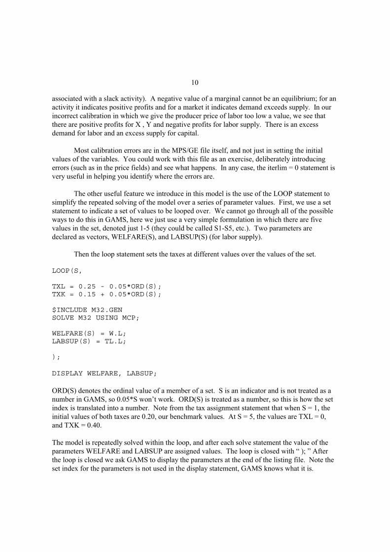
10

associated with a slack activity). A negative value of a marginal cannot be an equilibrium; for an

activity it indicates positive profits and for a market it indicates demand exceeds supply. In our

incorrect calibration in which we give the producer price of labor too low a value, we see that

there are positive profits for X , Y and negative profits for labor supply. There is an excess

demand for labor and an excess supply for capital.

Most calibration errors are in the MPS/GE file itself, and not just in setting the initial

values of the variables. You could work with this file as an exercise, deliberately introducing

errors (such as in the price fields) and see what happens. In any case, the iterlim = 0 statement is

very useful in helping you identify where the errors are.

The other useful feature we introduce in this model is the use of the LOOP statement to

simplify the repeated solving of the model over a series of parameter values. First, we use a set

statement to indicate a set of values to be looped over. We cannot go through all of the possible

ways to do this in GAMS, here we just use a very simple formulation in which there are five

values in the set, denoted just 1-5 (they could be called S1-S5, etc.). Two parameters are

declared as vectors, WELFARE(S), and LABSUP(S) (for labor supply).

Then the loop statement sets the taxes at different values over the values of the set.

LOOP(S,

TXL = 0.25 - 0.05*ORD(S);TXK = 0.15 + 0.05*ORD(S);


WELFARE(S) = W.L;LABSUP(S) = TL.L;

);

DISPLAY WELFARE, LABSUP;

ORD(S) denotes the ordinal value of a member of a set. S is an indicator and is not treated as a

number in GAMS, so 0.05*S won’t work. ORD(S) is treated as a number, so this is how the set

index is translated into a number. Note from the tax assignment statement that when S = 1, the

initial values of both taxes are 0.20, our benchmark values. At S = 5, the values are TXL = 0,

and TXK = 0.40.

The model is repeatedly solved within the loop, and after each solve statement the value of the

parameters WELFARE and LABSUP are assigned values. The loop is closed with “ ); ” After

the loop is closed we ask GAMS to display the parameters at the end of the listing file. Note the

set index for the parameters is not used in the display statement, GAMS knows what it is.

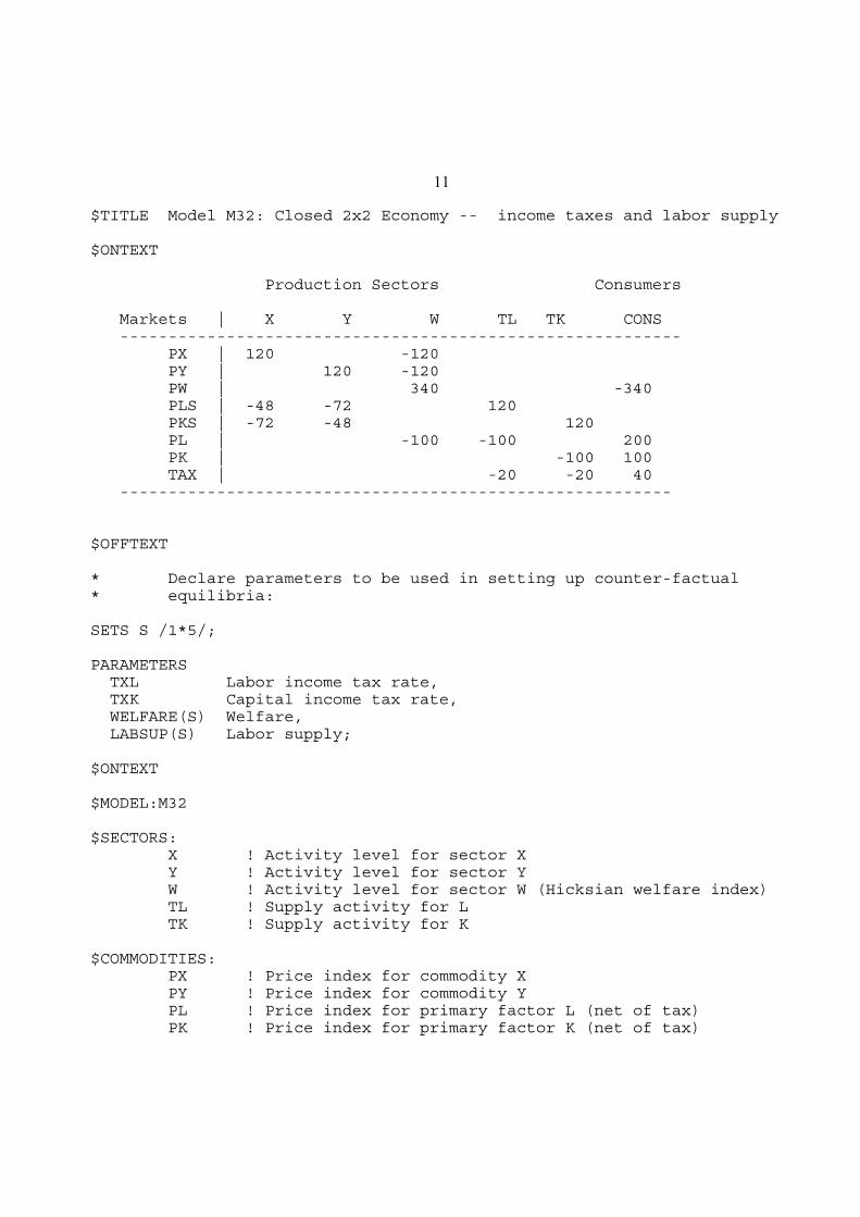
11

$TITLE Model M32: Closed 2x2 Economy -- income taxes and labor supply

$ONTEXT


Markets | X Y W TL TK CONS ---------------------------------------------------------- PX | 120 -120 PY | 120 -120 PW | 340 -340 PLS | -48 -72 120 PKS | -72 -48 120 PL | -100 -100 200 PK | -100 100 TAX | -20 -20 40 ---------------------------------------------------------

$OFFTEXT

* Declare parameters to be used in setting up counter-factual* equilibria:

SETS S /1*5/;

PARAMETERS TXL Labor income tax rate, TXK Capital income tax rate, WELFARE(S) Welfare, LABSUP(S) Labor supply;

$ONTEXT

$MODEL:M32

$SECTORS: X ! Activity level for sector X Y ! Activity level for sector Y W ! Activity level for sector W (Hicksian welfare index) TL ! Supply activity for L TK ! Supply activity for K

$COMMODITIES: PX ! Price index for commodity X PY ! Price index for commodity Y PL ! Price index for primary factor L (net of tax) PK ! Price index for primary factor K (net of tax)

12

PLS ! Price index for primary factor L (gross of tax) PKS ! Price index for primary factor K (gross of tax) PW ! Price index for welfare (expenditure function)


$PROD:X s:1 O:PX Q:120 I:PLS Q: 40 P:1.2 I:PKS Q: 60 P:1.2

$PROD:Y s:1 O:PY Q:120 I:PLS Q: 60 P:1.2 I:PKS Q: 40 P:1.2

$PROD:TL O:PLS Q:100 P:1.2 I:PL Q:100 P:1 A:CONS T:TXL

$PROD:TK O:PKS Q:100 P:1.2 I:PK Q:100 P:1 A:CONS T:TXK

$PROD:W s:0.7 a:1 O:PW Q:340 I:PX Q:120 a: I:PY Q:120 a: I:PL Q:100



* Benchmark replication:

TXL = 0.2;TXK = 0.2;

PW.FX = 1;

PX.L =1.; PY.L =1.; PLS.L =1.2; PKS.L =1.2;

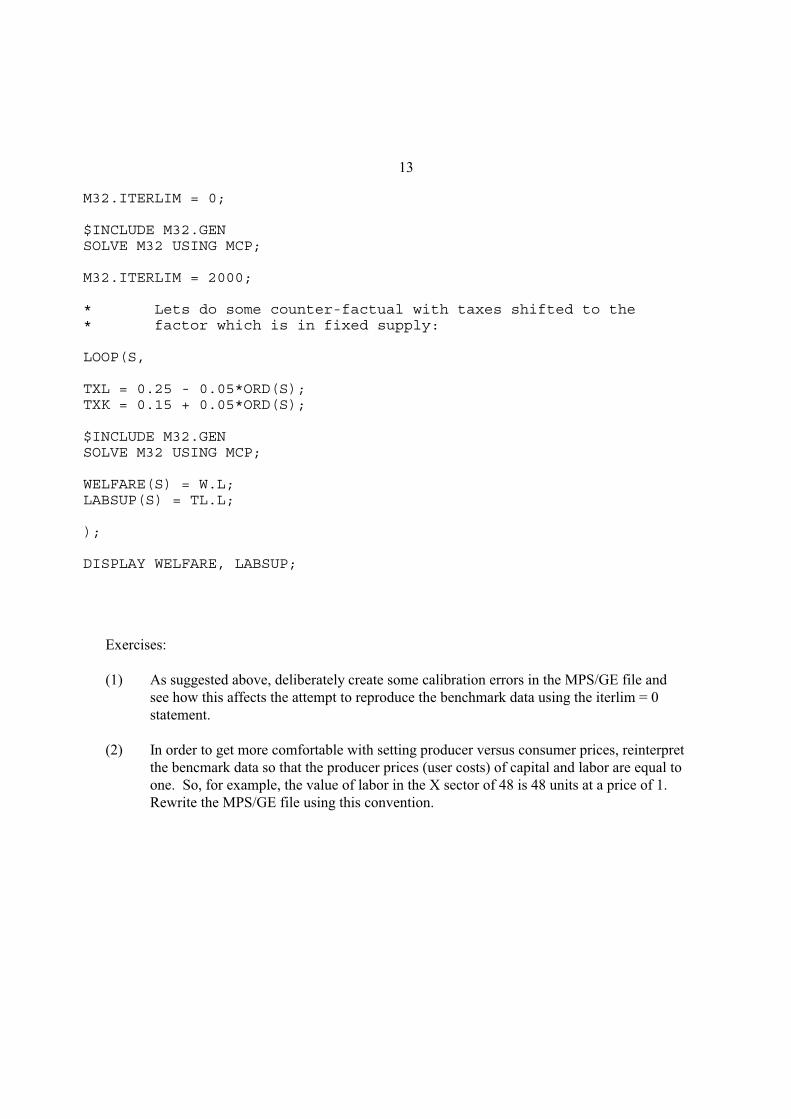
13

M32.ITERLIM = 0;


M32.ITERLIM = 2000;

* Lets do some counter-factual with taxes shifted to the* factor which is in fixed supply:

LOOP(S,

TXL = 0.25 - 0.05*ORD(S);TXK = 0.15 + 0.05*ORD(S);


WELFARE(S) = W.L;LABSUP(S) = TL.L;

);

DISPLAY WELFARE, LABSUP;

Exercises:

(1) As suggested above, deliberately create some calibration errors in the MPS/GE file and

see how this affects the attempt to reproduce the benchmark data using the iterlim = 0

statement.

(2) In order to get more comfortable with setting producer versus consumer prices, reinterpret

the bencmark data so that the producer prices (user costs) of capital and labor are equal to

one. So, for example, the value of labor in the X sector of 48 is 48 units at a price of 1.

Rewrite the MPS/GE file using this convention.

14

Model M33

This model is a follow-up on model M32 where we considered some income tax reform

experiments. Like that model, here we apply taxes through activities which transform (supply)

household owned factors into production inputs. The difference here is that we set up a model in

which we can do differential tax policy analysis holding the level of government revenue

constant. In order to keep things simple, we continue to rebate tax revenue in lump-sum fashion.

This model introduces a fourth (and final) class of MPSGE variables (in addition to

activity levels, commodity prices and income levels). The new entity is called an "auxiliary

variable". In this model, we use an auxiliary variable to endogenously alter the tax rate in order

to maintain an equal yield.

In the present case, we will hold the labor tax rate exogenous, but change its value, in

each case solving for the value of the capital tax that yields the same value of revenue as the

original tax. TXK now become a variable, not a parameter. In the initial MPS/GE statements

specifying the model, we declare a list of “auxiliary variables” (note the spelling of auxiliary, use

a double “l” and the model will crash), in this case a single variable TXK.

$AUXILIARY: TXK ! Endogenous capital tax from equal yield constraint.

This variable appears in the production block for capital supply as follows.

$PROD:TK O:PKS Q:100 P:1.2 I:PK Q:100 A:CONS N:TXK

N: is a new field in a production block, standing for eNdogenous tax rate followed by the

auxiliary variable. This is read in words as “assign to consumer CONS the revenue from an

endogenous tax rate TXK”. TXK is in turn associated with a constraint equation, which is

written in GAMS syntax but inside the MPS/GE block. Here is how we write it in this model.

$CONSTRAINT:TXK TXL*PL*TL*100 + TXK*PK*TK*100 =E= 40*(PX + PY)/2;

The left-hand side is tax revenue from the two taxes, one an exogenous parameter (TXL) and the

other an endogenous variable (TXK). Each term is (tax rate) x (factor price) x (activity level for

factor supply) x (the reference quantity supplied at an activity level equal to one).

The right-hand side of the constraint specifies the target revenue. With prices changing in

general equilibrium, the modeler has to think carefully about what is meant by “constant”

revenue: that is, constant in terms of what? Here we assume that the government wants the taxes

to yield an amount equal to the cost of purchasing given and equal amounts of X and Y, so for

15

example the initial tax revenue of 40 is spend (at prices for X and Y equal to one) on 20 X and 20

Y. The right-hand side of the constraint equation will continue to allow the purchase of

X = Y = 20 as the prices of the goods change in general equilibrium. Of course, the government

is not actually buying anything in this simple model, it is just redistributing the revenue back to

the consumer. But the point is that the modeler must specify what the revenue target is in real

terms, and then allow the nominal value of that to adjust with prices.

For historical reasons, the default values of auxiliary variables in MPS/GE are zero, not

one. So the modeler should set the initial values of these variables for the replication check even

if they should happen to be one. In our case, the initial value of TXK = 0.20, so we set this along

with the values of PLS and PKS which are equal to 1.2 initially, along with the initial value of

the parameter TXL (the latter is a parameter and so does not use the ‘.L’ syntax).

TXL = 0.20;TXK.L = 0.20;PLS.L = 1.2;PKS.L = 1.2;

After the replication check, we loop over values of TXL, and each solve statement finds the new

value of TXK as one variable in the new general-equilibrium solution.

In each iteration, we store the values of key variables so that they can be conveniently

presented together at the end of the listing file. We include the real value of commodity

consumption as discussed in Chapter 2, model M26, to show the difference between the effects

of the reform on real commodity consumption (REALCONS) and true welfare (WELFARE), the

latter accounting for changes in the value of leisure. Note from the results in the present case,

that measuring only the change in real commodity consumption significantly overstates the true

welfare gain of the tax reform (which is tiny) because of the fall in leisure (increase in labor

supply).

Finally, although the difference is small, note that the capital tax that needs to be

associated with TXL = 0 is TXK = 0.476, not the 0.50 value we assumed in the previous model

adjusting the capital and labor taxes one for one in opposite directions.

16

$TITLE Model M32: Closed 2x2 Economy -- Equal Yield Tax Reform

$ONTEXT


Markets | A B W TL TK CONS ---------------------------------------------------------- PX | 120 -120 PY | 120 -120 PW | 340 -340 PLS | -48 -72 120 PKS | -72 -48 120 100 PL | -100 -100 200 PK | -100 TAX | -20 -20 40 ---------------------------------------------------------

$OFFTEXT

SETS S /1*5/;

PARAMETERS TXL Labor income tax rate, WELFARE(S) Welfare, REALCONS(S) Real consumption of goods, LABSUP(S) Labor supply, CAPTAX(S) Capital tax rate;

$ONTEXT

$MODEL:M32

$SECTORS: X ! Activity level for sector X Y ! Activity level for sector Y W ! Activity level for sector W (Hicksian welfare index) TL ! Supply activity for L TK ! Supply activity for K

$COMMODITIES: PX ! Price index for commodity X PY ! Price index for commodity Y PL ! Price index for primary factor L (net of tax) PK ! Price index for primary factor K (net of tax) PLS ! Price index for primary factor L (gross of tax) PKS ! Price index for primary factor K (gross of tax)

17

PW ! Price index for welfare (expenditure function)


$AUXILIARY: TXK ! Endogenous capital tax from equal yield constraint.

$PROD:X s:1 O:PX Q:120 I:PLS Q: 40 P:1.2 I:PKS Q: 60 P:1.2

$PROD:Y s:1 O:PY Q:120 I:PLS Q: 60 P:1.2 I:PKS Q: 40 P:1.2

$PROD:TL O:PLS Q:100 P:1.2 I:PL Q:100 A:CONS T:TXL

$PROD:TK O:PKS Q:100 P:1.2 I:PK Q:100 A:CONS N:TXK

$PROD:W s:0.7 a:1 O:PW Q:340 I:PX Q:120 a: I:PY Q:120 a: I:PL Q:100


$CONSTRAINT:TXK TXL*PL*TL*100 + TXK*PK*TK*100 =E= 40 * (PX + PY)/2;


TXL = 0.20;

TXK.L = 0.20;

18

PLS.L = 1.2;PKS.L = 1.2;

M32.ITERLIM = 0;$INCLUDE M32.GENSOLVE M32 USING MCP;M32.ITERLIM = 2000;

LOOP(S,

TXL = 0.25 - 0.05*ORD(S);


WELFARE(S) = W.L;REALCONS(S) = (PX.L*X.L*120 + PY.L*Y.L*120) /(PX.L**0.5*PY.L**0.5*240);LABSUP(S) = TL.L;CAPTAX(S) = TXK.L;

);

DISPLAY WELFARE, REALCONS, LABSUP, CAPTAX;

19

Model 34

The assumption of lump-sum redistribution is a convenient trick which simplifies tax

policy analysis. In practice, governments often use money to purchase things which private

markets do not provide. People value the public provision, but for some reason it is not easy to

collect money from beneficiaries.

In this model, we first explicitly introduce government as an agent or “consumer”

(GOVT). The tax revenue collected in the economy is assigned to the government. The

government spends this on purchasing a good called G (price PG), which is produced from

capital and labor like the other goods X and Y. Here is the production block for G (all inputs in

all sectors are taxed at 25%) and the demand block for the consumer GOVT.

$PROD:G s:1 O:PG Q: 50 I:PL Q: 20 P:1.25 A:GOVT T:TAX I:PK Q: 20 P:1.25 A:GOVT T:TAX

$DEMAND:GOVT D:PG

The government is the only agent demanding PG in the model. As we noted back in

Chapter 1, MPS/GE transfers the tax revenue to the government in the background, this being the

government’s only source of income.

Now comes the tricky part. Each consumer receives the full benefit of the public good

without actually purchasing or paying for it. The community park is just there, free for the

consumer. How do we model this free transfer from the government to the consumer?

To do this, we introduce another feature of MPS/GE, the rationing variable and rationing

constraint. The rationing variable is declared as an auxiliary variable, denoted here LGP It

appears as a multiplier on an endowment field in a consumer’s demand equation. Here is the

correct syntax for the demand blocks for the two consumers.

$DEMAND:CONS1 D:PW1 Q:125 E:PL Q: 50 E:PK Q: 50 E:PG1 Q: 50 R:LGP


20

MPS/GE just multiplies the quantity in the Q field by the value of the variable in the R field, so

in this case CONS1 has an endowment of PG1 equal to 50*LGP.

The value of LGP, like any auxiliary variable is set by a constraint equation. In our case,

LGP takes on the value of G, the activity level for production of the public good. Note that 50 is

the reference quantity for the G activity at G = 1, so the auxiliary rationing variable LGP transfers

the full amount of the public good to each consumer.

$CONSTRAINT:LGP LGP =E= G;

Note that we have defined and used two different commodities for the public good

endowments of the two consumers, PG1 and PG2 respectively, even though each consumer is

getting the full (and therefore equal) amount of the public good. The reason that we do this is to

prevent the consumers from being able to trade the goods in the event that they have different

valuations of public good. One cannot sell his or her endowment of the public park to the other

consumer. These “personalized” endowments of the public good are then inputs to each

consumer’s welfare. Here are the two utility functions.

$PROD:W1 s:1 O:PW1 Q:125 I:PX Q: 70 I:PY Q: 30 I:PG1 Q: 50 P:0.5


Only consumer 1 is endowed wit PG1 and only consumer 1 demands PG1. Similar comments

apply to consumer 2 and PG2.

What about the valuations of the public goods at a price PG1 = PG2 = 0.5? We are going

to assume that the initial data represent an optimal initial provision of the public good.

According to the Samuelson rule, discussed in connection with the next model, the public good is

optimally provided with non-distortionary taxation if the cost of providing one unit equals the

sum of the demand prices, since each consumer consumes the full amount. This is satisfied here

if each consumer has a demand price of 0.5 in the initial benchmark situation.

Now we will give the full micro-consistent data matrix for this problem. Factor supplies

are taxes at 25% to all sectors.

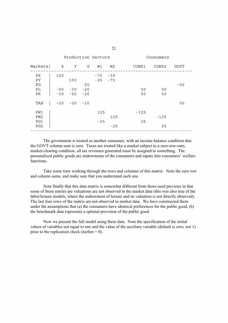
21


Markets| X Y G W1 W2 CONS1 CONS2 GOVT--------------------------------------------------------------- PX | 100 -70 -30 PY | 100 -30 -70 PG | 50 -50 PL | -50 -30 -20 50 50 PK | -30 -50 -20 50 50

TAX | -20 -20 -10 50

PW1 | 125 -125 PW2 | 125 -125 PG1 | -25 25 PG2 | -25 25---------------------------------------------------------------

The government is treated as another consumer, with an income balance condition that

the GOVT column sum is zero. Taxes are treated like a market subject to a zero-row-sum,

market-clearing condition: all tax revenues generated must be assigned to something. The

personalized public goods are endowments of the consumers and inputs into consumers’ welfare

functions.

Take some time working through the rows and columns of this matrix. Note the zero row

and column sums, and make sure that you understand each one.

Note finally that this data matrix is somewhat different from those used previous in that

some of these entries are valuations are not observed in the market data (this was also true of the

labor/leisure models, where the endowment of leisure and its valuation is not directly observed).

The last four rows of the matrix are not observed in market data. We have constructed them

under the assumptions that (a) the consumers have identical preferences for the public good, (b)

the benchmark data represents a optimal provision of the public good.

Now we present the full model using these data. Note the specification of the initial

values of variables not equal to one and the value of the auxiliary variable (default is zero, not 1)

prior to the replication check (iterlim = 0).

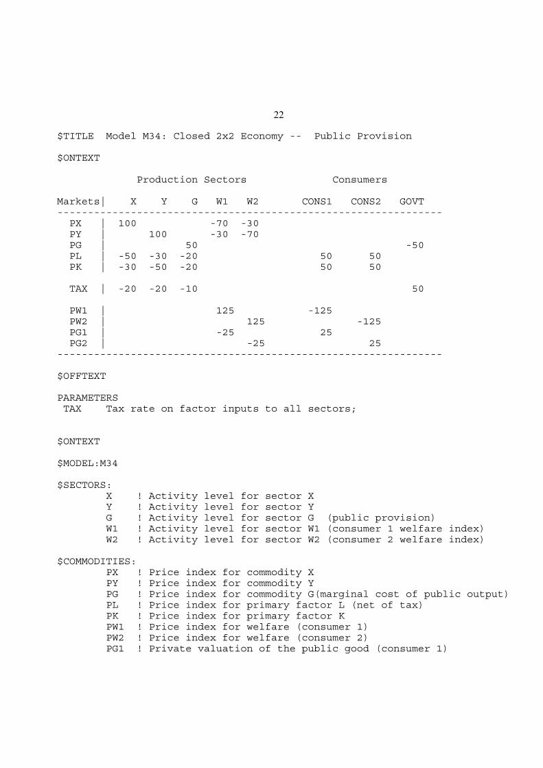
22

$TITLE Model M34: Closed 2x2 Economy -- Public Provision

$ONTEXT


Markets| X Y G W1 W2 CONS1 CONS2 GOVT--------------------------------------------------------------- PX | 100 -70 -30 PY | 100 -30 -70 PG | 50 -50 PL | -50 -30 -20 50 50 PK | -30 -50 -20 50 50

TAX | -20 -20 -10 50

PW1 | 125 -125 PW2 | 125 -125 PG1 | -25 25 PG2 | -25 25---------------------------------------------------------------

$OFFTEXT

PARAMETERS TAX Tax rate on factor inputs to all sectors;

$ONTEXT

$MODEL:M34

$SECTORS: X ! Activity level for sector X Y ! Activity level for sector Y G ! Activity level for sector G (public provision) W1 ! Activity level for sector W1 (consumer 1 welfare index) W2 ! Activity level for sector W2 (consumer 2 welfare index)

$COMMODITIES: PX ! Price index for commodity X PY ! Price index for commodity Y PG ! Price index for commodity G(marginal cost of public output) PL ! Price index for primary factor L (net of tax) PK ! Price index for primary factor K PW1 ! Price index for welfare (consumer 1) PW2 ! Price index for welfare (consumer 2) PG1 ! Private valuation of the public good (consumer 1)

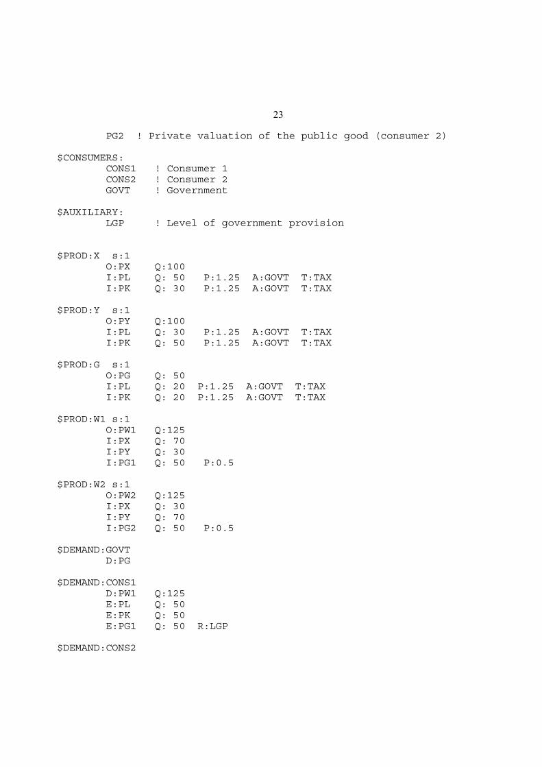
23

PG2 ! Private valuation of the public good (consumer 2)

$CONSUMERS: CONS1 ! Consumer 1 CONS2 ! Consumer 2 GOVT ! Government

$AUXILIARY: LGP ! Level of government provision

$PROD:X s:1 O:PX Q:100 I:PL Q: 50 P:1.25 A:GOVT T:TAX I:PK Q: 30 P:1.25 A:GOVT T:TAX

$PROD:Y s:1 O:PY Q:100 I:PL Q: 30 P:1.25 A:GOVT T:TAX I:PK Q: 50 P:1.25 A:GOVT T:TAX

$PROD:G s:1 O:PG Q: 50 I:PL Q: 20 P:1.25 A:GOVT T:TAX I:PK Q: 20 P:1.25 A:GOVT T:TAX



$DEMAND:GOVT D:PG


$DEMAND:CONS2

24

D:PW2 Q:125 E:PL Q: 50 E:PK Q: 50 E:PG2 Q: 50 R:LGP



TAX = 0.25;LGP.L = 1;PG1.L = 0.5;PG2.L = 0.5;


* The following counterfactuals check that the original* benchmark is indeed an optimum by raising/lowering the tax

TAX = 0.20;


TAX = 0.30;


Exercises:

(1) Define a set, parameters, and write a loop statement over finer values of the tax rate (e.g.,

1% steps) storing the welfare of each consumer for each tax rate. See if the tax of 25% is

optimal.

(2) Change one consumer’s valuation of the public good. The first run of the model should

reproduce the benchmark data, but one consumer will prefer a different tax rate. Conduct

the same experiment as in (1) with the new valuation and see what happens from the

point of view of each consumer.

25

Model 35

This model is exactly the same as the previous one, except that the tax used to finance the

public good is endogenous. Thus we will not repeat the data matrix here, and most other

elements of the model are already familiar.

Instead of TAX being a parameter, it is now an auxiliary variable. Its value is set by the

constraint equation:

$CONSTRAINT:TAX PG =E= PG1 + PG2;

This is a condition noted by Samuelson many years ago. Since each consumer gets the

full amount of the public good (the good is “non-rivaled”), the marginal benefit of another unit of

the good is the sum of the demand prices for all the consumers. Efficiency is achieved when this

sum of benefits is equal to the marginal cost of producing another unit. This is given by the

above equation.

Note that the auxiliary variable itself need not appear in the constraint equation associated

with it. The solution algorithm will adjust TAX in order to satisfy this condition.

Strictly speaking, the Samuelson rule is valid only if the tax needed to pay for the public

good can be raised in a non-distortionary way. If distortionary taxes must be used, the sum of

marginal benefits must be weighed against the marginal cost of production plus the marginal

burden of taxation. It is beyond the scope of this chapter to discuss this problem further here.

When we run this model, we will get back a value of TAX = 0.25, because we calibrated

the prefences assuming that the initial data was optimal. As a counterfactual experiment, we

change one consumer’s valuation of the public good, using a parameter VG1 which is a

multiplier on consumer 1's initial valuation of the good.

$PROD:W1 s:1 O:PW1 Q:125 I:PX Q: 70 I:PY Q: 30 I:PG1 Q: 50 P:(0.5*VG1)

In the counterfactual experiment we double consumer 1's “willingness to pay”, setting

VG1 = 2. Here are some results from the counterfactual.

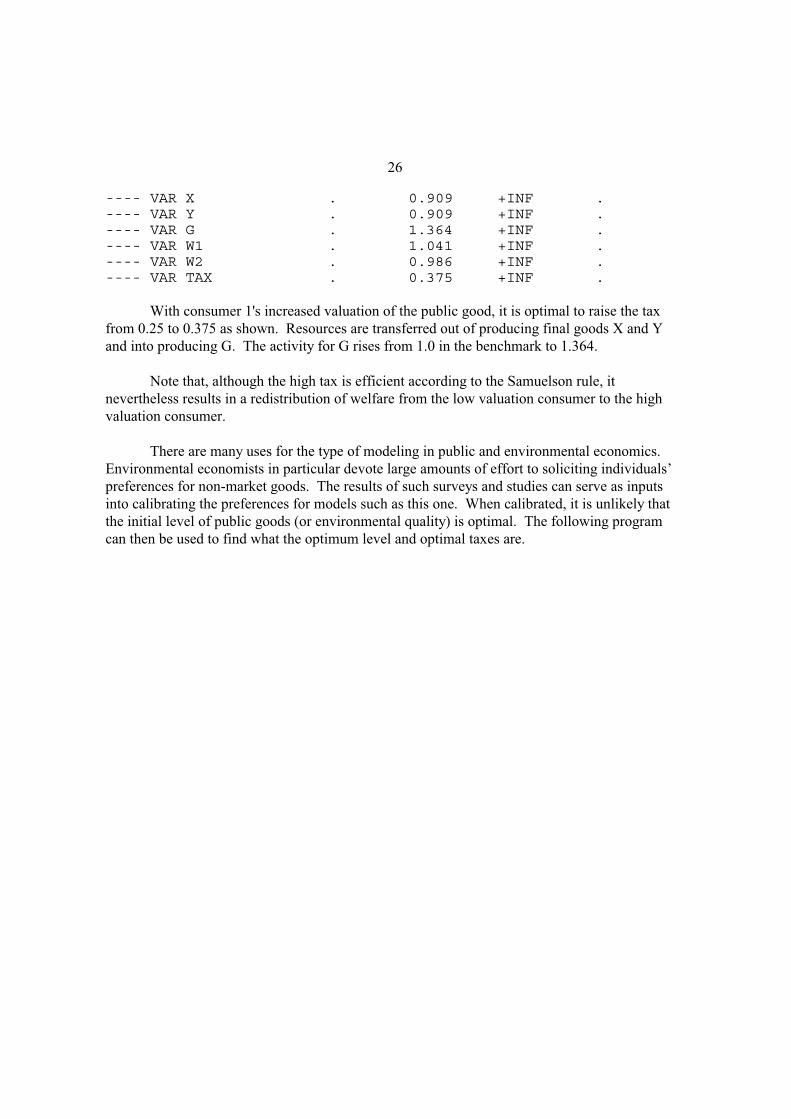
26

---- VAR X . 0.909 +INF .---- VAR Y . 0.909 +INF .---- VAR G . 1.364 +INF .---- VAR W1 . 1.041 +INF .---- VAR W2 . 0.986 +INF .---- VAR TAX . 0.375 +INF .

With consumer 1's increased valuation of the public good, it is optimal to raise the tax

from 0.25 to 0.375 as shown. Resources are transferred out of producing final goods X and Y

and into producing G. The activity for G rises from 1.0 in the benchmark to 1.364.

Note that, although the high tax is efficient according to the Samuelson rule, it

nevertheless results in a redistribution of welfare from the low valuation consumer to the high

valuation consumer.

There are many uses for the type of modeling in public and environmental economics.

Environmental economists in particular devote large amounts of effort to soliciting individuals’

preferences for non-market goods. The results of such surveys and studies can serve as inputs

into calibrating the preferences for models such as this one. When calibrated, it is unlikely that

the initial level of public goods (or environmental quality) is optimal. The following program

can then be used to find what the optimum level and optimal taxes are.

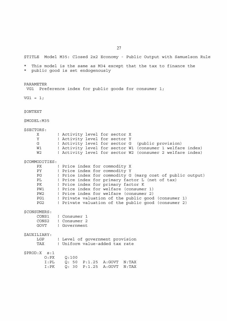
27

$TITLE Model M35: Closed 2x2 Economy - Public Output with Samuelson Rule

* This model is the same as M34 except that the tax to finance the * public good is set endogenously

PARAMETER VG1 Preference index for public goods for consumer 1;

VG1 = 1;

$ONTEXT

$MODEL:M35

$SECTORS: X ! Activity level for sector X Y ! Activity level for sector Y G ! Activity level for sector G (public provision) W1 ! Activity level for sector W1 (consumer 1 welfare index) W2 ! Activity level for sector W2 (consumer 2 welfare index)

$COMMODITIES: PX ! Price index for commodity X PY ! Price index for commodity Y PG ! Price index for commodity G (marg cost of public output) PL ! Price index for primary factor L (net of tax) PK ! Price index for primary factor K PW1 ! Price index for welfare (consumer 1) PW2 ! Price index for welfare (consumer 2) PG1 ! Private valuation of the public good (consumer 1) PG2 ! Private valuation of the public good (consumer 2)

$CONSUMERS: CONS1 ! Consumer 1 CONS2 ! Consumer 2 GOVT ! Government

$AUXILIARY: LGP ! Level of government provision TAX ! Uniform value-added tax rate

$PROD:X s:1 O:PX Q:100 I:PL Q: 50 P:1.25 A:GOVT N:TAX I:PK Q: 30 P:1.25 A:GOVT N:TAX

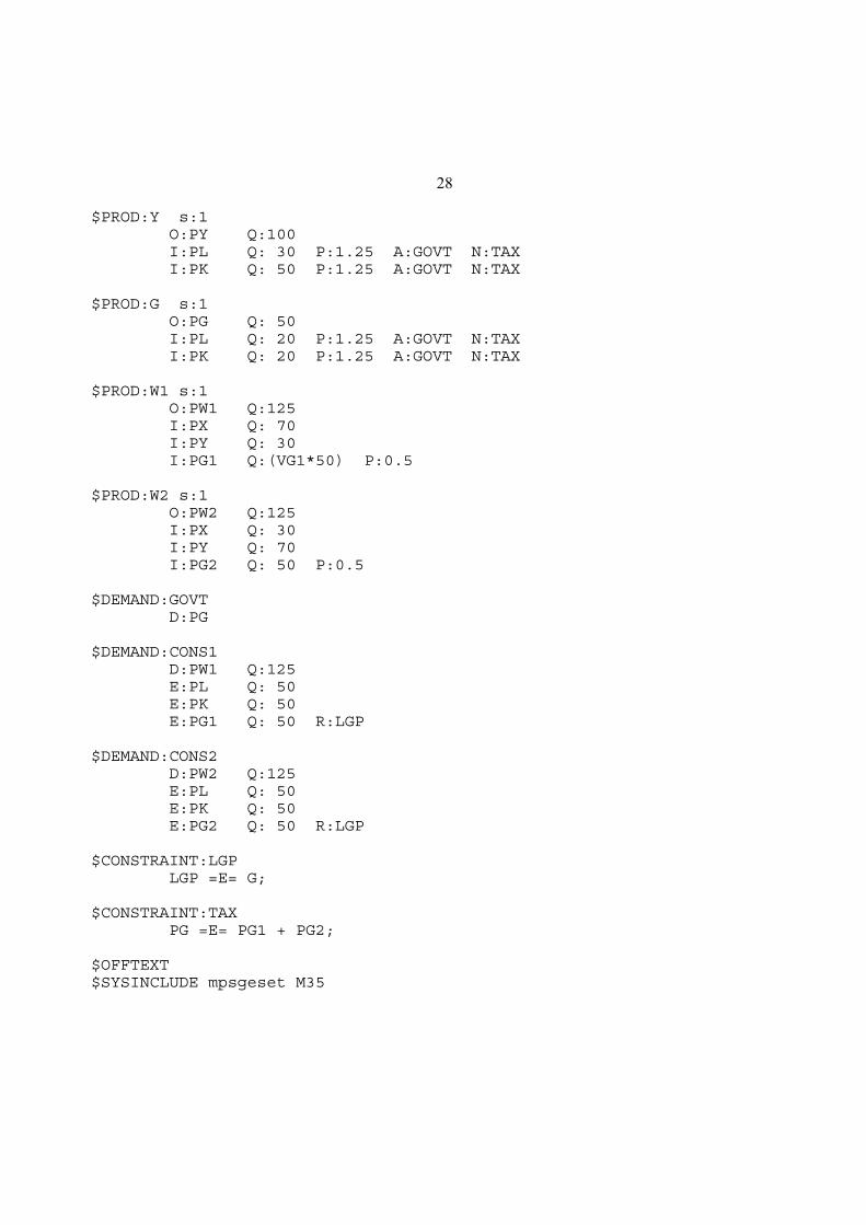
28

$PROD:Y s:1 O:PY Q:100 I:PL Q: 30 P:1.25 A:GOVT N:TAX I:PK Q: 50 P:1.25 A:GOVT N:TAX

$PROD:G s:1 O:PG Q: 50 I:PL Q: 20 P:1.25 A:GOVT N:TAX I:PK Q: 20 P:1.25 A:GOVT N:TAX

$PROD:W1 s:1 O:PW1 Q:125 I:PX Q: 70 I:PY Q: 30 I:PG1 Q:(VG1*50) P:0.5


$DEMAND:GOVT D:PG




$CONSTRAINT:TAX PG =E= PG1 + PG2;


29

* Benchmark replication

TAX.L = 0.25;LGP.L = 1;PG1.L = 0.5;PG2.L = 0.5;


* What happens to consumer 2 welfare if consumer 1 decides* she would like more public output:

VG1 = 2;


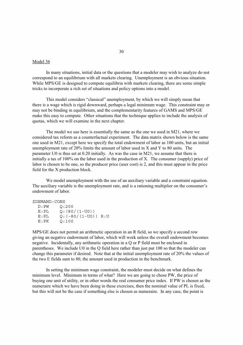
30

Model 36

In many situations, initial data or the questions that a modeler may wish to analyze do not

correspond to an equilibrium with all markets clearing. Unemployment is an obvious situation.

While MPS/GE is designed to compute equilibria with markets clearing, there are some simple

tricks to incorporate a rich set of situations and policy options into a model.

This model considers “classical” unemployment, by which we will simply mean that

there is a wage which is rigid downward, perhaps a legal minimum wage. This constraint may or

may not be binding in equilibrium, and the complementarity features of GAMS and MPS/GE

make this easy to compute. Other situations that the technique applies to include the analysis of

quotas, which we will examine in the next chapter.

The model we use here is essentially the same as the one we used in M21, where we

considered tax reform as a counterfactual experiment. The data matrix shown below is the same

one used in M21, except here we specify the total endowment of labor as 100 units, but an initial

unemployment rate of 20% limits the amount of labor used in X and Y to 80 units. The

parameter U0 is thus set at 0.20 initially. As was the case in M21, we assume that there is

initially a tax of 100% on the labor used in the production of X. The consumer (supply) price of

labor is chosen to be one, so the producer price (user cost) is 2, and this must appear in the price

field for the X production block.

We model unemployment with the use of an auxiliary variable and a constraint equation.

The auxiliary variable is the unemployment rate, and is a rationing multiplier on the consumer’s

endowment of labor.

$DEMAND:CONS D:PW Q:200 E:PL Q:(80/(1-U0)) E:PL Q:(-80/(1-U0)) R:U E:PK Q:100

MPS/GE does not permit an arithmetic operation in an R field, so we specify a second row

giving an negative endowment of labor, which will work unless the overall endowment becomes

negative. Incidentally, any arithmetic operation in a Q or P field must be enclosed in

parentheses. We include U0 in the Q field here rather than just put 100 so that the modeler can

change this parameter if desired. Note that at the initial unemployment rate of 20% the values of

the two E fields sum to 80, the amount used in production in the benchmark.

In setting the minimum wage constraint, the modeler must decide on what defines the

minimum level. Minimum in terms of what? Here we are going to chose PW, the price of

buying one unit of utility, or in other words the real consumer price index. If PW is chosen as the

numeraire which we have been doing in these exercises, then the nominal value of PL is fixed,

but this will not be the case if something else is chosen as numeraire. In any case, the point is

31

that the modeler should make a conscious choice of the numeraire for the minimum wage rate.

In many countries it is periodically adjusted to reflect changes in the consumer price index, and

PW is of course the theoretically ideal consumer price index.

Since units are chosen such that the prices PL and PW are initially equal to one, the

constraint equation setting the value of the auxiliary variable U is given by:

$CONSTRAINT:UPL =G= PW;

Running the model verifies that we have benchmarked it correctly, and that the initial

unemployment rate is 20%.

For a counterfactual experiment, we introduce a tax reform as in Model 21, and replace

the 100% tax on labor in X with equal tax rates of 25% on both factors (although this is still a

distortionary tax. Now run the model. Some of the results are as follows:


---- VAR X . 1.178 +INF .---- VAR Y . 1.106 +INF .---- VAR W . 1.142 +INF .---- VAR PX . 0.969 +INF .---- VAR PY . 1.032 +INF .---- VAR PL . 1.051 +INF .---- VAR PK . 1.005 +INF .---- VAR PW 1.000 1.000 1.000 EPS---- VAR CONS . 228.374 +INF .---- VAR U . . +INF 0.051

The minimum wage ceases to be binding (PL = 1.051) and unemployment falls to zero

(note that the marginal on U is the excess of PL over PW). There is a very large increase in

welfare, which goes to 1.142 as the increases in employment reinforces the tax reform. There are

some very interesting policy economics in this example. Initially, we have two distortions that

are reinforcing one another. If we reform the tax structure, the second distortion is automatically

removed by making it non-binding.

To see this effect, we do one final counterfactual in the model, which is to fix the

unemployment rate at its initial value of 20%, but allow the tax reform. If you look at the listing

file, you will see that welfare rises to only 1.021. Most of the effect of the tax reform shown

above is its indirect effect in eliminating the binding minimum wage constraint.

32

$TITLE Model M36: Closed 2x2 Economy - Taxes and Classical Unemployment

$ONTEXT


Markets | X Y W | CONS ------------------------------------------------------ PX | 100 -100 | PY | 100 -100 | PW | 200 | -200 PL | -20 -60 | 100*(1-U) PK | -60 -40 | 100 TAX | -20 0 | 20 ------------------------------------------------------

$OFFTEXT

PARAMETERS TX Proportional output tax on sector X, TY Proportional output tax on sector Y, TLX Ad-valorem tax on labor inputs to X, TKX Ad-valorem tax on capital inputs to X, U0 Initial unemployment rate;

U0 = 0.20;

$ONTEXT

$MODEL:M36




$AUXILIARY:U ! Unemployment rate

33

$PROD:X s:1 O:PX Q:100 A:CONS T:TX I:PL Q: 20 P:2 A:CONS T:TLX I:PK Q: 60 A:CONS T:TKX

$PROD:Y s:1 O:PY Q:100 T:TY I:PL Q: 60 I:PK Q: 40


$DEMAND:CONS D:PW Q:200 E:PL Q:(80/(1-U0)) E:PL Q:(-80/(1-U0)) R:U E:PK Q:100

$CONSTRAINT:UPL =G= PW;


PW.FX = 1;

TX = 0;TY = 0;TLX = 1;TKX = 0;U.L = U0;


* As in M31, we replace the tax on labor inputs* by a uniform tax on both factors:

TLX = 0.25;TKX = 0.25;TX = 0;TY = 0;

34


U.FX = 0.20;


Exercises:

(1) Try a different numeraire for defining the minimum wage and see what happens.

(2) If you want to be a little bit more ambitious, try adding a labor-leisure decision to the

problem.

35

Model 37

As in the case of labor supply, we would like to have models in which the stock of capital

is endogenous. This requires dynamic modeling, a significant complication of what we have

done to this point. This chapter will not consider true dynamic modeling. However, we will

present a shortcut that is very valuable in many situations. In models for which there exists a

steady state, it is possible to represent this steady state as a complementarity problem not that

different from our static models. We can then at least perform comparative steady-state

experiments, in which a parameter change moves us from one steady state to another. But

actually solving for the transition path requires a more complicated analysis that is postponed

until later in the book.

Model 37 incorporates optimal capital accumulation via the use of a rationing constraint

and endogenous “taxes” to create a model for comparative steady state analysis when the capital

stock is endogenously adjusted to its steady-state value. The labor force is assumed fixed in this

model.

Let r denote the rental price (for one period) of a unit of capital and let pk denote the price

of a new unit of capital. will denote the rate of depreciation of capital per period, and will

denote the discount rate between periods. The steady-state optimal capital accumulation

condition is a relationship between the price and rental rate on capital. The rental rate must be

given by:

r 11

1p

k

The rental price (r) is equal to the price of creating a new unit of capital (pk) minus the present

value of what the capital could be sold for next period. In the steady state, the price of a new unit

next period is the same, so an old unit can be sold for its original value minus one period’s

depreciation (1 - ). The present value of the undepreciated portion is thus (1 - )/(1+ ).

The dynamic steady-state problem is represented as a static problem using two tricks.

First, the use of capital is subsidized to create the desired wedge (denoted TAU) between the

rental price and the price of new capital. Following the declaration of the parameters DELTA,

RHO, and TAU you will see:

TAU = - (1 - DELTA) / (1 + RHO);

This then appears as a subsidy to capital use, creating the wedge between the rental price and the

price of producing a new unit of capital (PK).

$PROD:X s:1 O:PX Q:100 I:PL Q: 40

36

I:PK Q:120 P:0.5 A:CONS T:TAU

$PROD:Y s:1 O:PY Q:100 I:PL Q: 60 I:PK Q: 80 P:0.5 A:CONS T:TAU

One unit of new capital is produced using one unit of labor, as you will see in the

production block for activity K.

Second, since in the steady state newly produced capital is equal to depreciation and

depreciation is equal to a share DELTA of total capital, a rationing constraint is specified to

"endow" consumers with the carryforward from the previous period. Let Ks denote the capital

stock and Kn the production of new capital. In the steady state, these are related by:

Kn

Ks

Ks

Kn

1

The carryforward from the previous period is the steady state stock minus new production. It is

is called KFORWD and given by:

carry forward = KFORWD = Ks

Kn

Kn

Kn

(1 )Kn

So in the model below, we will give the consumer an endowment, via the rationing multiplier

KFORWD, the quantity of capital on the right-hand side of the above equation.

$DEMAND:CONS D:PW E:PL Q:160 E:PK Q:1 R:KFORWRD

$CONSTRAINT:KFORWRD KFORWRD =E= K * (1-DELTA) / DELTA;

That completes the model description. As has been our practice, we include the initial

micro-consistent data matrix in the program. Study this carefully in going through the program.

Note that in the data matrix, the consumer is “endowed” with 140 units of capital. In the

program, this is the carry forward and is subject to change in counterfactual experiments.

Two counterfactuals are run in the program. First the rate of time preference is raised.

In the second, is set back to its initial value, and there is a tax on new capital production. See if

you can guess what the effects of these changes should be, and then look at the results.

37

$TITLE Model M38: Closed 2x2 Economy - Steady State Capital Stock

$ONTEXT


Markets | X Y K W | CONS ------------------------------------------------------ PX | 100 -100 | PY | 100 -100 | PW | 200 | -200 PL | -40 -60 -60 | 160 PK | -120 -80 60 | 140 SUB | 60 40 | -100 ------------------------------------------------------

$OFFTEXT

PARAMETERS RHO Time preference parameter, DELTA Depreciation rate, TAU Effective capital use tax (it is a subsidy, its < 0), KTAX Tax on new capital production NEWCAP New capital stock after counterfactual (= 1 initially);

RHO = 0.4;DELTA = 0.3;TAU = - (1 - DELTA) / (1 + RHO);KTAX = 0;

$ONTEXT

$MODEL:M37

$SECTORS: X ! Activity level for sector X Y ! Activity level for sector Y W ! Activity level for sector W (Hicksian welfare index) K ! Capital stock index


38


$AUXILIARY: KFORWRD ! Capital stock from previous period

$PROD:X s:1 O:PX Q:100 I:PL Q: 40 I:PK Q:120 P:0.5 A:CONS T:TAU

$PROD:Y s:1 O:PY Q:100 I:PL Q: 60 I:PK Q: 80 P:0.5 A:CONS T:TAU

$PROD:K O:PK Q:1 A:CONS T:KTAX I:PL Q:1


$DEMAND:CONS D:PW E:PL Q:160 E:PK Q:1 R:KFORWRD

$CONSTRAINT:KFORWRD KFORWRD =E= K * (1-DELTA) / DELTA;


K.L = 60;KFORWRD.L = 140;PW.FX = 1;


39

* Raise the rate of time preference from 0.4 to 0.6:

RHO = 0.6;TAU = - (1 - DELTA) / (1 + RHO);


NEWCAP = K.L/60;DISPLAY NEWCAP;

* Set rho back to 0.4, tax new capital at 0.20

RHO = 0.4;TAU = - (1 - DELTA) / (1 + RHO);

KTAX = 0.20;


NEWCAP = K.L/60;DISPLAY NEWCAP;

Exercises:

(1) Make sure you understand the economic intuition behind the results in the

counterfactuals.

(2) If you are ambitious, write a new model combining endogenous labor supply and an equal

yield tax constraint with this model. Do some experiments to see if the capital tax or the

labor tax is more distortionary. This is an important use of applied modeling: theory can

never tell you which of two distortionary taxes is more distortionary.

1

Chapter 4:

Open Economy models

Naturally, a very important task for the modeler is building open economy models, since

trade and international investment policies are among the important policy problems facing

governments. This chapter continues in the spirit of the previous chapters, presenting a series of

simple models which incorporate features of open economy issues one by one. Here are the

model names with brief descriptions of their features.

M41.GMS Small open economy 2x2

M42.GMS Small open economy with a benchmark tariff

M43.GMS Same as M42 except with a different price normalization

M44.GMS Small open economy with a benchmark quota

M45.GMS Small open economy with a benchmnark voluntary export restraint

M46.GMS Small open economy with a benchmark trade imbalance

M47.GMS An Armington formulation

M48.GMS Large open economy

M49.GMS Full two-country Heckscher-Ohlin model

M410.GMS International capital flows

Model 41

This is a very simple 2-good, 2-factor model in which the rest of the world is not

explicitly modeled. Trading opportunities are summarized by simple functions which allow the

economy to transform one good (an export) into another (an import). The “technology” of these

functions represents world prices. If good X1 exchanges for two units of X2, then the world price

ratio is implicitly given by p1/p2 = 2. We will assume that these technologies or price ratios are

fixed in this model and the first few models to follow. This is commonly know as the “small-

country assumption”: the country can trade as much or as little as it wants at fixed prices.

We assume in the benchmark data that the country exports X1 in exchange for X2, but we

will allow for the fact that some policy or endowment change could actually reverse the direction

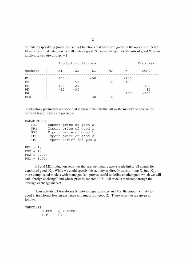
2

of trade by specifying (initially inactive) functions that transform goods in the opposite direction.

Here is the initial data, in which 50 units of good X1 are exchanged for 50 units of good X2 at an

implicit price ratio of p1/p2 = 1.

Production Sectors Consumer

Markets | X1 X2 E1 M2 W CONS----------------------------------------------------------------P1 | 150 -50 -100P2 | 50 50 -100PL | -100 -20 120PK | -50 -30 80PW | 200 -200PFX | 50 -50----------------------------------------------------------------

Technology parameters are specified in these functions that allow the modeler to change the

terms of trade. These are given by:

PARAMETERS PE2 Export price of good 2, PM1 Import price of good 1, PE1 Export price of good 1, PM2 Import price of good 2, TM2 Import tariff for god 2;

PE1 = 1;PM2 = 1;PE2 = 0.99;PM1 = 1.01;

E1 and M2 production activities that are the initially active trade links. E1 stands for

exports of good X1 . While we could specify this activity as directly transforming X1 into X2 , in

more complicated models with many goods it proves useful to define another good which we will

call “foreign exchange” and whose price is denoted PFX. All trade is mediated through the

“foreign exchange market”.

Thus activity E1 transforms X1 into foreign exchange and M2, the import activity for

good 2, transforms foreign exchange into imports of good 2. These activities are given as

follows:

$PROD:E1 O:PFX Q:(50*PE1) I:P1 Q:50

3

$PROD:M2 O:P2 Q:50 I:PFX Q:(50*PM2) A:CONS T:TM2

TM2 is an import tariff on good 2, which is initially set to zero. We also specify trade

links in the opposite direction, which are initially inactive as noted above. At this point, we have

an opportunity to make an important technical remark which may save the modeler some misery

later on. Suppose that good 1 can be transformed into good 2 at a price of one, and good 2 can

be transformed into good 1 at a price of 1. Then if the export of 50 units of good 1 and imports

of 50 units of good 2 is an equilibrium, then so is the export of 100 units of good 1 followed by

the imports of 50 units of good 2 plus 50 units of good 1.

In technical terms the model is “degenerate”, it has infinitely many solutions. In such a

situation, the solver will either fail to converge, or converge to an arbitrary solution. The latter

will have net exports (exports minus imports) of X1 equal to 50 and net imports of X2 equal to

50, but may involve any amount of gross trade.

This is why we specify the prices or “terms of trade” differently for the activities M1 and

E2, so that it is never profitable to export and import the same good.

Here is the model. In the first counterfacual we impose a tariff and 5% and then a tariff

of 10%. When you look at the listing files, you will see that the tariff of 10% is prohibitive, all

trade ceases. The last experiment returns the tariff to zero, and improves the terms of trade

(relative prices of the export good) to 1.2.

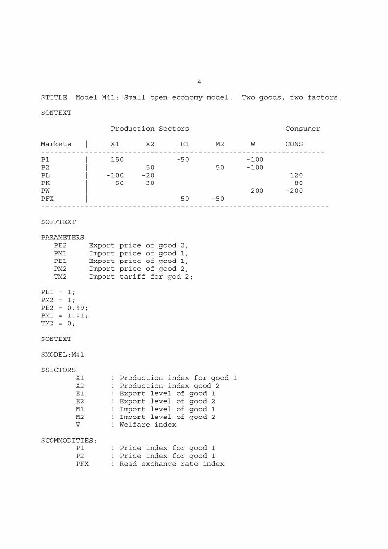
4

$TITLE Model M41: Small open economy model. Two goods, two factors.

$ONTEXT


Markets | X1 X2 E1 M2 W CONS-----------------------------------------------------------------P1 | 150 -50 -100P2 | 50 50 -100PL | -100 -20 120PK | -50 -30 80PW | 200 -200PFX | 50 -50------------------------------------------------------------------

$OFFTEXT

PARAMETERS PE2 Export price of good 2, PM1 Import price of good 1, PE1 Export price of good 1, PM2 Import price of good 2, TM2 Import tariff for god 2;

PE1 = 1;PM2 = 1;PE2 = 0.99;PM1 = 1.01;TM2 = 0;

$ONTEXT

$MODEL:M41

$SECTORS: X1 ! Production index for good 1 X2 ! Production index good 2 E1 ! Export level of good 1 E2 ! Export level of good 2 M1 ! Import level of good 1 M2 ! Import level of good 2 W ! Welfare index

$COMMODITIES: P1 ! Price index for good 1 P2 ! Price index for good 1 PFX ! Read exchange rate index

5

PW ! Welfare price index PL ! Wage index PK ! Capital rental index

$CONSUMERS: CONS ! Income level for representative agent

$PROD:X1 s:1 O:P1 Q:150 I:PL Q:100 I:PK Q: 50

$PROD:X2 s:1 O:P2 Q:50 I:PL Q:20 I:PK Q:30




$PROD:M1 O:P1 Q:50 I:PFX Q:(50*PM1)

$PROD:W s:1 O:PW Q:200 I:P1 Q:100 I:P2 Q:100

$DEMAND:CONS D:PW Q:200 E:PL Q:120 E:PK Q: 80


PW.FX = 1;

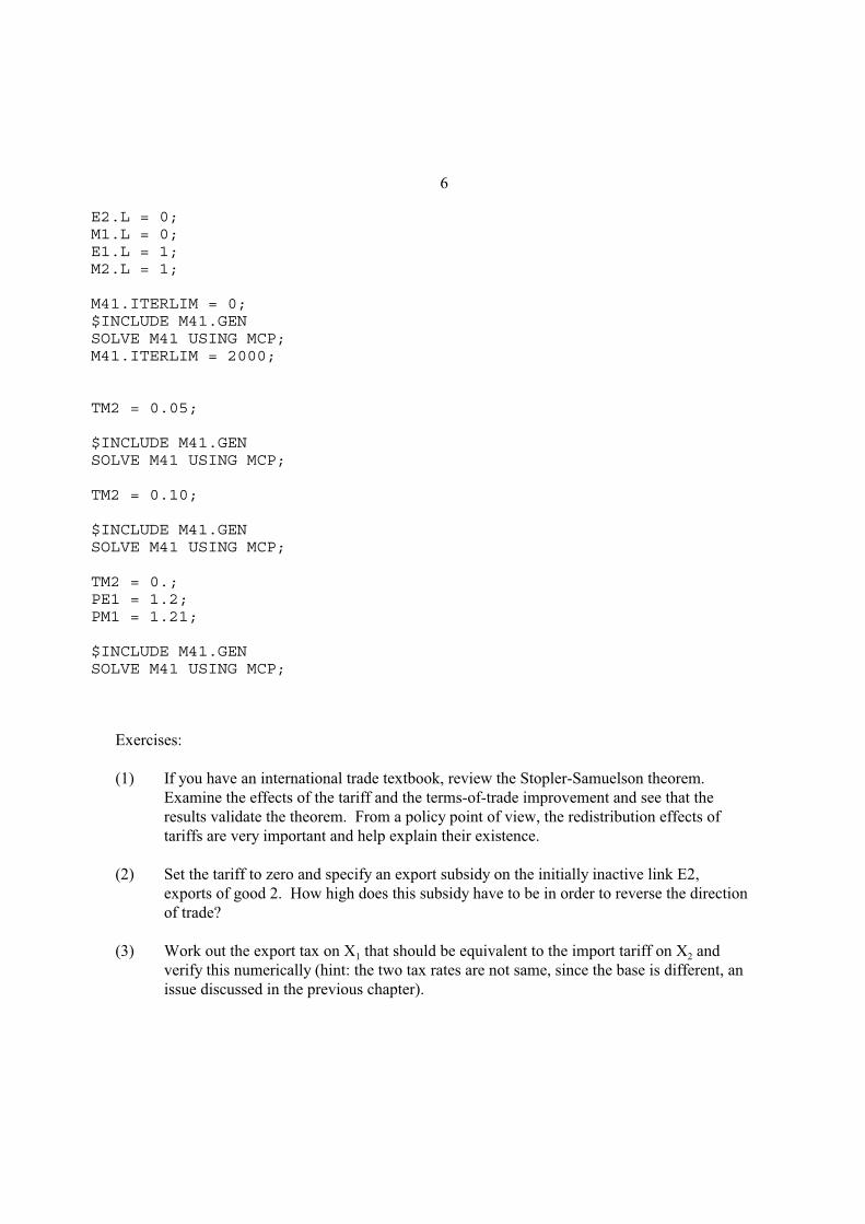
6

E2.L = 0;M1.L = 0;E1.L = 1;M2.L = 1;


TM2 = 0.05;


TM2 = 0.10;


TM2 = 0.;PE1 = 1.2;PM1 = 1.21;


Exercises:

(1) If you have an international trade textbook, review the Stopler-Samuelson theorem.

Examine the effects of the tariff and the terms-of-trade improvement and see that the

results validate the theorem. From a policy point of view, the redistribution effects of

tariffs are very important and help explain their existence.

(2) Set the tariff to zero and specify an export subsidy on the initially inactive link E2,

exports of good 2. How high does this subsidy have to be in order to reverse the direction

of trade?

(3) Work out the export tax on X1 that should be equivalent to the import tariff on X2 and

verify this numerically (hint: the two tax rates are not same, since the base is different, an

issue discussed in the previous chapter).

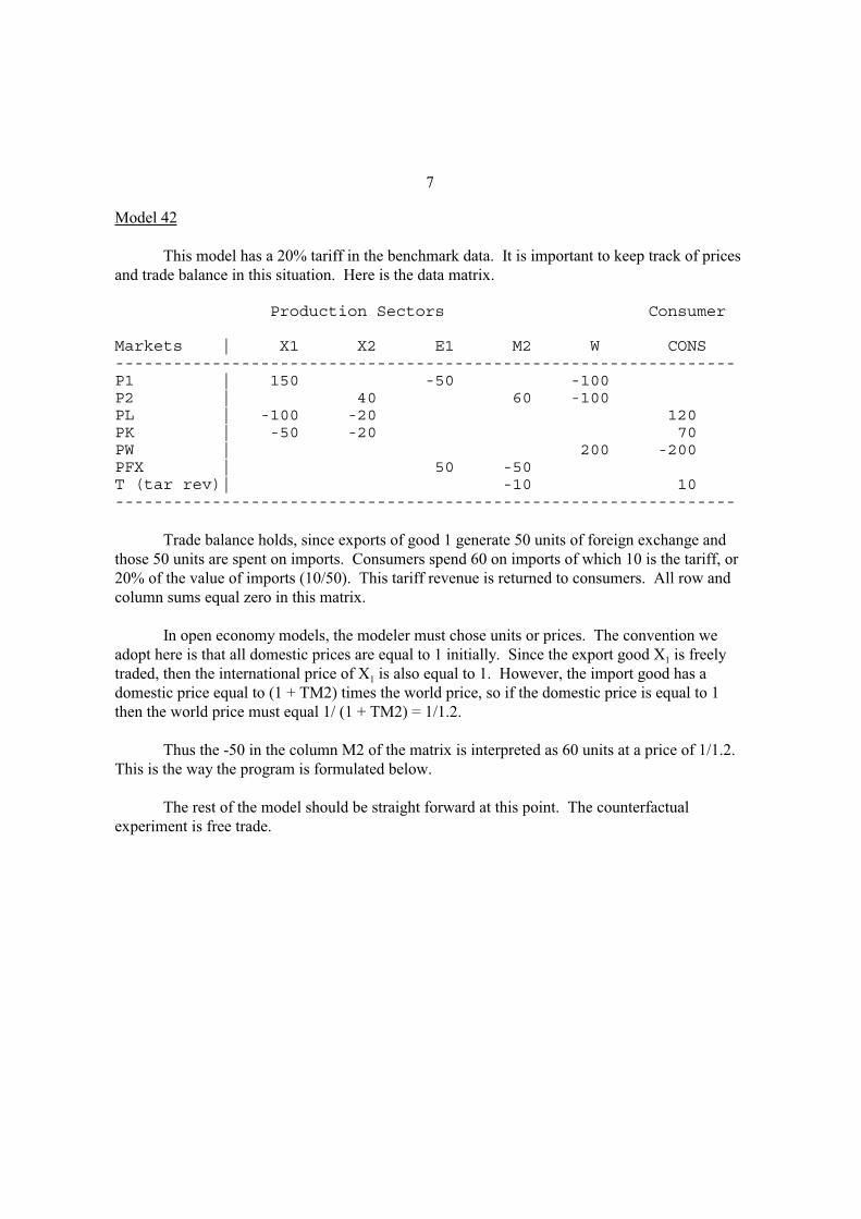
7

Model 42

This model has a 20% tariff in the benchmark data. It is important to keep track of prices

and trade balance in this situation. Here is the data matrix.


Markets | X1 X2 E1 M2 W CONS----------------------------------------------------------------P1 | 150 -50 -100P2 | 40 60 -100PL | -100 -20 120PK | -50 -20 70PW | 200 -200PFX | 50 -50T (tar rev)| -10 10----------------------------------------------------------------

Trade balance holds, since exports of good 1 generate 50 units of foreign exchange and

those 50 units are spent on imports. Consumers spend 60 on imports of which 10 is the tariff, or

20% of the value of imports (10/50). This tariff revenue is returned to consumers. All row and

column sums equal zero in this matrix.

In open economy models, the modeler must chose units or prices. The convention we

adopt here is that all domestic prices are equal to 1 initially. Since the export good X1 is freely

traded, then the international price of X1 is also equal to 1. However, the import good has a

domestic price equal to (1 + TM2) times the world price, so if the domestic price is equal to 1

then the world price must equal 1/ (1 + TM2) = 1/1.2.

Thus the -50 in the column M2 of the matrix is interpreted as 60 units at a price of 1/1.2.

This is the way the program is formulated below.

The rest of the model should be straight forward at this point. The counterfactual

experiment is free trade.

8

$TITLE Model M42: Small open economy model with a benchmark tariff.

$ONTEXT

In this example, units are chosen such that all DOMESTIC prices equalone initially. Implied world prices are then P1/P2 = 1.2


Markets | X1 X2 E1 M2 W CONS------------------------------------------------------------------P1 | 150 -50 -100P2 | 40 60 -100PL | -100 -20 120PK | -50 -20 70PW | 200 -200PFX | 50 -50T (tar rev)| -10 10------------------------------------------------------------------

$OFFTEXT

PARAMETERS

PE2 Export price of good 2, PM1 Import price of good 1, PE1 Export price of good 1, PM2 Import price of good 2, TM2 Import tariff for good 2;

PE1 = 1;PM2 = 1/(1.2);PE2 = PM2*0.99;PM1 = 1.01;TM2 = 0.20;

$ONTEXT

$MODEL:M42

$SECTORS: X1 ! Production index for good 1 X2 ! Production index good 2 E1 ! Export level of good 1 E2 ! Export level of good 2 M1 ! Import level of good 1

9

M2 ! Import level of good 2 W ! Welfare index

$COMMODITIES: P1 ! Price index for good 1 P2 ! Price index for good 1 PFX ! Read exchange rate index PW ! Welfare price index PL ! Wage index PK ! Capital rental index









$DEMAND:CONS D:PW Q:200 E:PL Q:120

10

E:PK Q: 70


PW.FX = 1;

E1.L = 1;M2.L = 1;E2.L = 0;M1.L = 0;


* Counterfactual experiment is free trade

TM2 = 0;


Model M43

In models with many countries, the modeler may wish to choose world prices as all

equaling 1. Model M43 is exactly the same as model M42 except that we choose world prices as

1. This only affects the calibration via the choice of units for X2 . Since the world price of good

2 is equal to 1, then the domestic price is P2 = 1.2. But if this is the case, then the value of X2

production (40) and consumption (100) must imply benchmark quantities of

40 = 1.2*(quantity) quantity = 33.3333

100 = 1.2*(quantity) quantity = 83.3333

You will see these numbers in the quantity fields of the program. W for example, is calibrated

as:

$PROD:W s:1 O:PW Q:200 I:P1 Q:100 I:P2 Q:83.33333 P:1.2

Other features of the model are identical to M42 as noted, so here is the program.

11

$TITLE Model M43: Small open economy model with a benchmark tariff.* alternaive price normalization from M42

$ONTEXT

This model is equivalent to M42 except that units are chosen suchthat all WORLD prices equal one initially. The benchmark domestic priceratio is then P2 = 1.2.

Note that this changes the units of measurement in good 2. There arenow 83.3333 units of good 2 consumed instead of 100, but this is simplya change in units of measure and has no welfare consequences.


Markets | X1 X2 E1 M2 W CONS------------------------------------------------------------------P1 | 150 -50 -100P2 | 40 60 -100PL | -100 -20 120PK | -50 -20 70PW | 200 -200PFX | 50 -50T | -10 10------------------------------------------------------------------

$OFFTEXT

PARAMETERS


PE1 = 1;PM2 = 1;PE2 = 0.99;PM1 = 1.01;TM2 = 0.20;

$ONTEXT

$MODEL:M43

12




* Cobb-Douglas production in both sectors:


$PROD:X2 s:1 O:P2 Q:33.33333 P:1.2 I:PL Q:20 I:PK Q:20



$PROD:E2 O:PFX Q:(50*PE2) I:P2 Q:(50)


13

$PROD:W s:1 O:PW Q:200 I:P1 Q:100 I:P2 Q:83.33333 P:1.2



PW.FX = 1;


E1.L = 1;M2.L = 1;E2.L = 0;M1.L = 0;P2.L = 1.2;



TM2 = 0;


Exercise:

Choices of units with which to interpret the data is a dull, but important step. Many calibration

problems (failure to replicate the data as an initial equilibrium) can be traced to mistakes over

price and quantity units when there are taxes or quotas in the initial data. So spend some time

comparing this file to M42. Run the models and verify that all results on activity levels and

welfare are the same.

14

Model 44

This model assumes the same benchmark data as the previous two models, but it assumes

that there is a quota limiting imports. A quota is a quantitative restriction on imports, generally a

maximum restriction although there could conceivably be a minimum quota. The former

generates a gap between the foreign or world supply price and the domestic demand price for the

“rationed” good. This difference, often referred to as a quota rent (it is a form of Ricardian rent),

must go to some agent.

In this model, we assume that the government implements the quota via the creation of

licenses. These licenses may be auctioned off, sometimes referred to as an auction quota. Or

they may simply be given out to some agents inside the economy. Since we have only a single

representative household in this model, the model cannot really distinguish between these two.

But in a model with several households it can produce an important difference. Indeed, quota

licenses are sometimes a source of corruption in real economies, generating rents for favored

individuals (the license owners) without them having to produce anything at all.

Using a trick that may now seem familiar from earlier models, we use an auxiliary

variable, Q, for an endogenous tax rate and a constraint equation to set the value of this “tax”.

The revenue from this tax is assigned to the representative consumer in the block for the import

demand for M2.

$PROD:M2 O:P2 Q:60 I:PFX Q:(60*PM2) A:CONS N:Q

The constraint equation says to set the value of the tax Q such that the activity level for imports

(calibrated to be 1 initially) is equal to 1.

$CONSTRAINT:Q 1 =G= M2;

Other aspects of the model should be familiar. We return here to the convention of model

42 that units are chosen such that all domestic prices equal 1. The counterfactual experiment is

to set the quota equal to zero. This is done with the statement Q.FX = 0; since Q is a variable,

not a parameter. An alternative way to do this is to declare a parameter and use it in place of the

‘1’ on the left-hand side of the constraint equation. Then the quota can be set at any level.

The value of Q can be thought of as the tariff equivalent of the quota or the “shadow

tariff”. In one exercise following the model, you are asked to increase the size of the economy

and see what happens to this shadow tariff. To free up a variable when it has been fixed, use:

Q.L = 0;Q.UP = +INF.

15

$TITLE Model M44: Small open economy model with a (auction) quota

$ONTEXT

In this example, units are chosen such that all DOMESTIC prices equalone initially. Implied world prices are then P1/P2 = 1.2


Markets | X1 X2 E1 M2 W CONS------------------------------------------------------------------P1 | 150 -50 -100P2 | 40 60 -100PL | -100 -20 120PK | -50 -20 70PW | 200 -200PFX | 50 -50Q (quota rent)| -10 10------------------------------------------------------------------

$OFFTEXT

PARAMETERS


PE1 = 1;PM2 = 1/(1.2);PE2 = PM2*0.99;PM1 = 1.01;TM2 = 0.20;

$ONTEXT

$MODEL:M42

$SECTORS: X1 ! Production index for good 1 X2 ! Production index good 2 E1 ! Export level of good 1 E2 ! Export level of good 2 M1 ! Import level of good 1 M2 ! Import level of good 2

16

W ! Welfare index



$AUXILIARY: Q




$PROD:M2 O:P2 Q:60 I:PFX Q:(60*PM2) A:CONS N:Q




17




PW.FX = 1;

E1.L = 1;M2.L = 1;E2.L = 0;M1.L = 0;Q.L = 0.20;



Q.FX = 0;


Exercises:

(1) Free up the quota again (begin with the statements Q.L0 = 0; Q.UP = +INF;

where ‘LO’ stands for lower bound and ‘UP’ stands for upper bound). Double factor

endowments. (You can declare a parameter that is multiplied by the factor endowments

as in model M1_MPS.) See what happens to the shadow tariff, the value of Q. Can you

explain why?

(2) Following this experiment, fix Q at Q = 0.20, its initial value so that it is in fact a tariff.

Again double the size of the economy and compare the results of this tariff experiment to

the quota experiment.

18

Model M45

In some cases, countries impose a so-called voluntary export restraint (VER), which asks

a foreign country or foreign firms to limit their exports to a certain quota level. The effect of this

is to transfer the quota rents to the foreign country. It is like having a tariff and giving the tariff

revenue to the foreign government. In order to model this, we introduce a second consumer,

denoted CONSF where F is for foreign and label the domestic consumer as CONSH. CONSF

receives the quota rent (shadow tariff revenue) and demands some of the country’s export good,

X1. Here the numbers we use:


Markets | X1 X2 E1 M2 W CONSH CONSF----------------------------------------------------------------P1 | 150 -50 -90 -10P2 | 40 60 -100PL | -100 -20 120PK | -50 -20 70PW | 190 -190PFX | 50 -50Q (ver) | -10 10----------------------------------------------------------------

This data is implemented in exactly the manner used in the previous example. We

declare an auxiliary variable V, which appears in an N (endogenous tax) field on the import

activity, and a constraint equation setting the value of V.

In order to compare this to the auction quota of the previous example, we also declare an

auxiliary quota variable Q which is an endogenous tax paid to the domestic consumer, and set by

a second constraint equation. In the initial benchmark run of the model, we set Q to zero, Q.FX

= 0; and replicate the bechmark. For our first counterfactual, we replace the VER with the quota

using the syntax noted in the previous model:

Q.LO = 0;Q.UP = +INF;V.FX = 0;

Run the model and examine the results. The equilibria are quite different and the shadow

values (Q and V) are not the same. The switch to the auction quota creates an income effect

which leads the domestic consumer to demand more goods and more imports at initial prices.

But more imports cannot occur under the quota, so in effect the quota becomes more restrictive

and the shadow tariff increases (Q is larger than V). Note that the welfare effect of switching

from the VER to the quota is quite large.

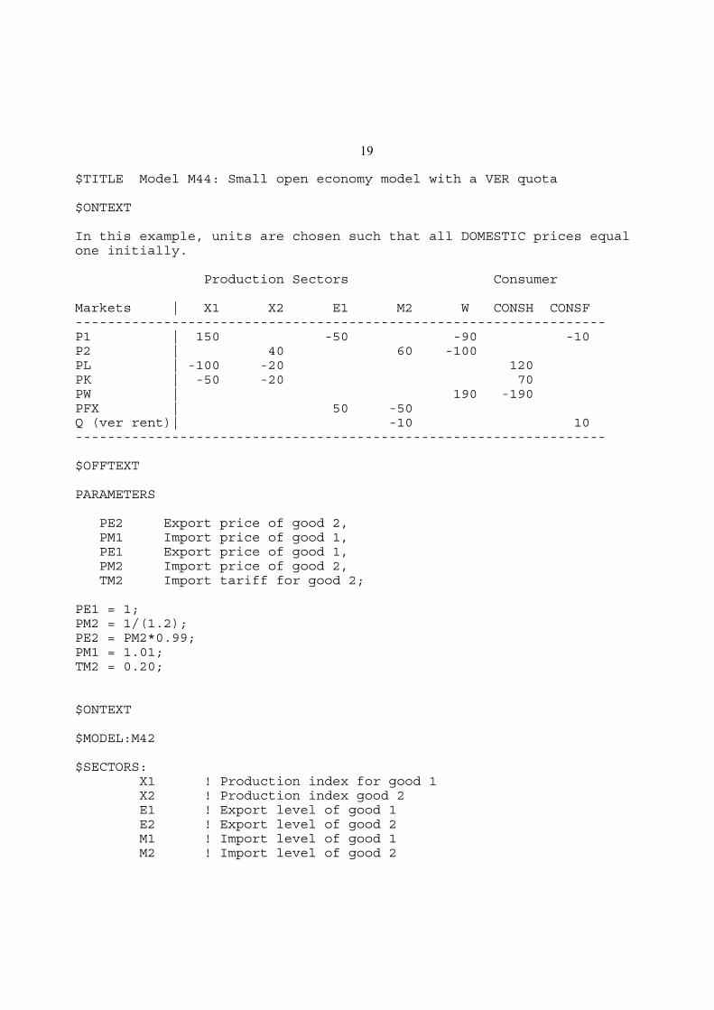
19

$TITLE Model M44: Small open economy model with a VER quota

$ONTEXT

In this example, units are chosen such that all DOMESTIC prices equalone initially.


Markets | X1 X2 E1 M2 W CONSH CONSF------------------------------------------------------------------P1 | 150 -50 -90 -10P2 | 40 60 -100PL | -100 -20 120PK | -50 -20 70PW | 190 -190PFX | 50 -50Q (ver rent)| -10 10------------------------------------------------------------------

$OFFTEXT

PARAMETERS


PE1 = 1;PM2 = 1/(1.2);PE2 = PM2*0.99;PM1 = 1.01;TM2 = 0.20;

$ONTEXT

$MODEL:M42

$SECTORS: X1 ! Production index for good 1 X2 ! Production index good 2 E1 ! Export level of good 1 E2 ! Export level of good 2 M1 ! Import level of good 1 M2 ! Import level of good 2

20

W ! Welfare index


$CONSUMERS: CONSH ! Income level for domestic consumer CONSF ! Income level for foreign consumer (quota holder)

$AUXILIARY: V ! Endogenous tax, shadow tax for VER Q ! Endogenous tax, shadow tax for quota




$PROD:M2 O:P2 Q:60 I:PFX Q:(60*PM2) A:CONSF N:V A:CONSH N:Q



$PROD:W s:1 O:PW Q:190 I:P1 Q: 90 I:P2 Q:100

21

$DEMAND:CONSH D:PW Q:190 E:PL Q:120 E:PK Q: 70

$DEMAND:CONSF D:P1 Q:10

$CONSTRAINT:V 1 =G= M2;



PW.FX = 1;

E1.L = 1;M2.L = 1;E2.L = 0;M1.L = 0;V.L = 0.20;Q.FX = 0;


* Counterfactual: replace the VER with an auction quota

Q.LO = 0;Q.UP = +INF;V.FX = 0;


Exercise:

Replace the initial VER with a tariff of 0.20 on the import good. Assign the tariff revenue to

agent CONSF. Show that this replicates the benchmark data. Show that a tariff of 0.20 assigned

to CONSH does not replicated the auction quota calculated in the counterfactual. Why not?

22

Model M46

Real economies are dynamic and therefore real economies can run trade imbalances in

any period by buying or selling assets. Any real data that a modeler is likely to encounter will

almost surely have a current account surplus or deficit in any one period. Yet static models are

useful for policy analysis and dynamic models are costly to construct in terms of time and data.

When a modeler wants to construct a static model starting with data characterized by a

trade imbalance, the model has several choices. These are sometime referred to as “closure

rules”. Some closure rules allow the trade balance to vary when doing counterfactuals. The

problem with this practice is that it makes welfare effects difficult to interpret. If a policy

experiment leads to an increase in the deficit, welfare will increase due, in fact, to foreign

borrowing. This is misleading, since at some point that borrowing will have to be paid back.

In general, we prefer to hold the deficit fixed when doing counterfactuals in static models,

so as to produce more easily interpreted welfare results. Model M46 shows how to do this.

The simplest trick is to just assume that the representative consumer has an initial

endowment of foreign exchange equal to the deficit. We can think of this as the amount of

foreign borrowing in the initial benchmark equilibrium. This is then held constant in any

counterfactual experiments. An initial surplus can be represented by a negative endowment of

PFX in the benchmark, denoting foreign lending.

This is what we do below. Benchmark exports are 40, imports are 60, and the deficit is

financed by selling the initial benchmark endowment of 20 units of PFX. The latter is specified

by the parameter BOPDEF which we can change in counterfactual experiments.

$DEMAND:CONS D:PW Q:220 E:PL Q:120 E:PK Q: 80 E:PFX Q:BOPDEF

For a counterfactual, we eliminate the deficit, setting BOPDEF = 0. Obviously, welfare is

going to fall.

This leads us to a short discussion about another modeling technique. Sometimes,

modelers have good reason to believe that the benchmark data is not an equilibrium, or wish to

conduct experiments starting from some other benchmark situation. In such situations, the

modeler can compute a “revised benchmark” by eliminating the source of disequilibrium to

generate a new benchmark data set. In the present case, if the modeler wanted to start with a

situation of a zero balance of trade, the model can then benchmark the model as we have done,

and then run the model with BOPDEF = 0. The new equilibrium values of activities, prices, and

income then become the new data set or “revised benchmark” for policy analysis.

23

$TITLE Model M46: Small open economy model with a benchmark trade * imbalance.

$ONTEXT


Markets | X1 X2 E1 M2 W CONS------------------------------------------------------------------P1 | 150 -40 -110P2 | 50 60 -110PL | -100 -20 120PK | -50 -30 80PW | 220 -220PFX | 40 -60 20------------------------------------------------------------------

$OFFTEXT

PARAMETERS PE2 Export price of good 2, PM1 Import price of good 1, PE1 Export price of good 1, PM2 Import price of good 2, TM2 Import tariff for good 2, BOPDEF Balance of payments net deficit;

PE1 = 1;PM2 = 1;PE2 = 0.99;PM1 = 1.01;TM2 = 0;

$ONTEXT

$MODEL:M46


$COMMODITIES: P1 ! Price index for good 1

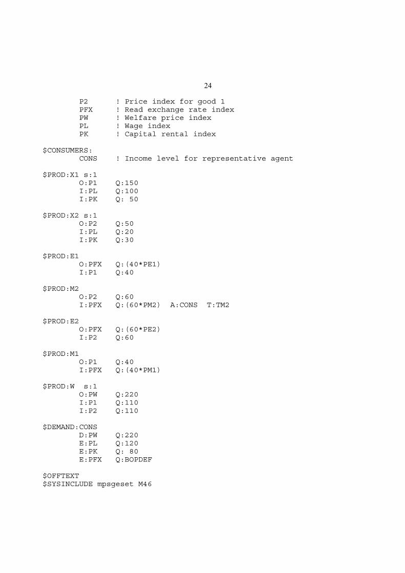
24

P2 ! Price index for good 1 PFX ! Read exchange rate index PW ! Welfare price index PL ! Wage index PK ! Capital rental index









$DEMAND:CONS D:PW Q:220 E:PL Q:120 E:PK Q: 80 E:PFX Q:BOPDEF


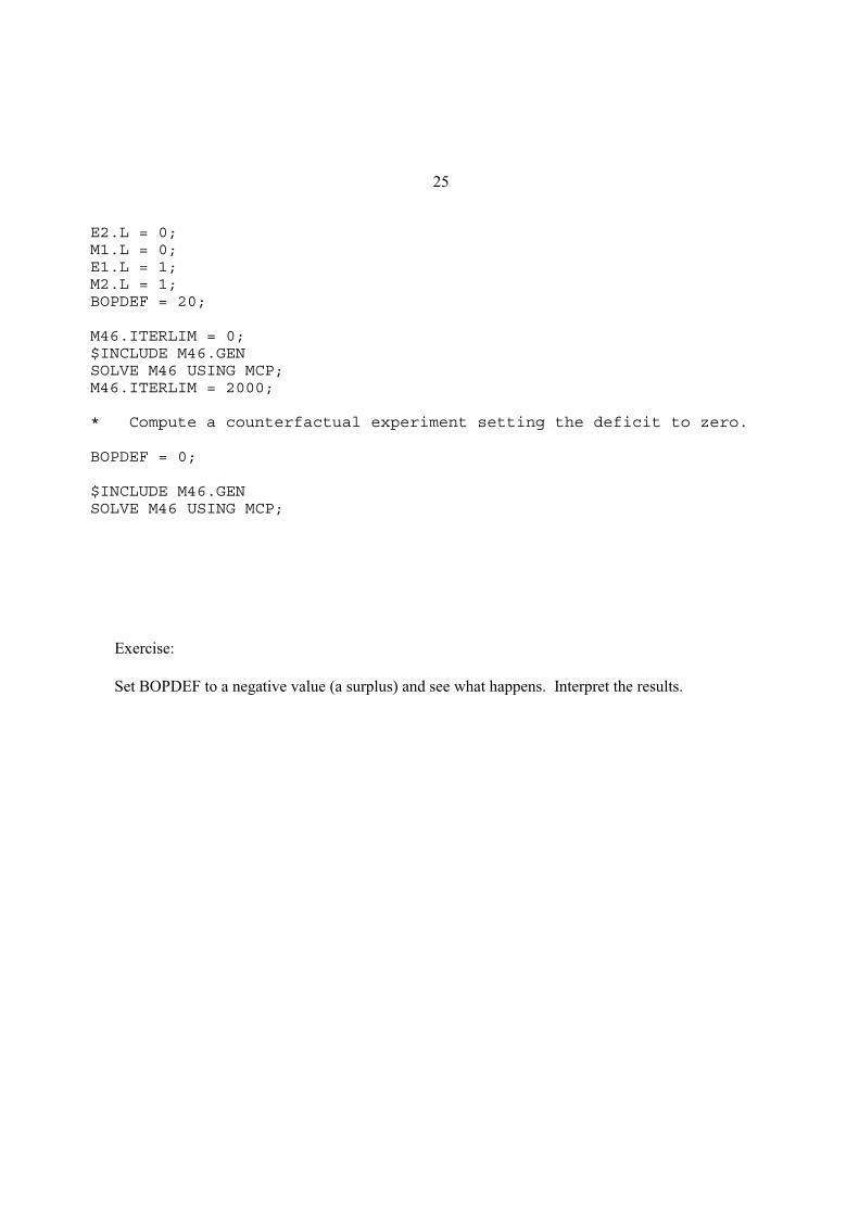
25

E2.L = 0;M1.L = 0;E1.L = 1;M2.L = 1;BOPDEF = 20;


* Compute a counterfactual experiment setting the deficit to zero.

BOPDEF = 0;


Exercise:

Set BOPDEF to a negative value (a surplus) and see what happens. Interpret the results.

26

Model 47

Another feature of real data that confronts modelers is that there is generally two-way

trade in any “good” in the data; that is, each good is both imported and exported. This is often

attributed to the fact that data is actually classified by industries and any industry is actually an

aggregation of many goods. Yet two-way trade or “cross hauling” will persist in the data even at

an extremely fine level of disaggregation. No research will ever get data that is free of cross

hauling so the question is what to do about it.

Model 47 is calibrated to the following data:


Markets | X1 X2 E M W CONS---------------------------------------------------------------P1 | 150 -100 50 -100P2 | 50 -25 75 -100PL | -100 -20 120PK | -50 -30 80PW | 200 -200PFX | 125 -125---------------------------------------------------------------

Each “good” (industry) is both imported and exported. One way to handle this is to

simply net out the two way trade from the gross flows and replace the data with net trade only. If

we do this in the present model, we arrive exactly at model M41. We can then proceed as before.

The other alternative in competitive models is to assume that the domestic and foreign

goods are not really identical. This is the so-called Armington assumption: domestic and foreign

goods in the same industrial classification are imperfect substitutes. This is really quite simple

for us in MPS/GE. We do not have to do anything on the production side or in the demand

blocks. Indeed, all that we have to do is to change the preferences to define four distinct goods

and a nesting structure for the utility function. In our case we write this as:

$PROD:W s:1 G1:ESUB G2:ESUB O:PW Q:200 I:P1 Q: 50 G1: I:PF1 Q: 50 G1: I:P2 Q: 25 G2: I:PF2 Q: 75 G2:

The modeler is completely free to choose any nesting structure of course, but this is a

common thing to do. The domestic (P1) and foreign good (PF1) in industry 1 are in a nest as are

the domestic and foreign goods in industry 2 and these nest have the same elasticity of

substitution: a domestic and foreign good in the same industry have the same substitution

27

elasticity regardless of industry. The composite industry 1 good and the composite industry 2

good are then combined in an upper level nest. This is generally assumed to have a lower

elasticity of substitution: two industries are poor substitutes than a domestic and foreign good in

the same industry. Here we specify the upper nest with an elasticity of substitution of 1, while

the domestic-foreign goods have an elasticity of substitution of ESUB = 4.

Other assumptions are possible, such as grouping all foreign goods together in a nest and

all domestic goods in another. But the procedure just outlined seems reasonable to many

modelers.

The rest of the program is rather familiar, except that the four trade activities are now

defined for four distinct goods. There is no need now to worry about a domestic good being both

imported and exported. It cannot, by definition, be imported.

After the replication check, we run the same counterfactuals that we did for model M41, a

tariff of 5% and then 10% on (foreign) good 2.

28

$TITLE Model M47: Small open economy model with an Armington * formulation.

$ONTEXT


Markets | X1 X2 E M W CONS---------------------------------------------------------------P1 | 150 -100 50 -100P2 | 50 -25 75 -100PL | -100 -20 120PK | -50 -30 80PW | 200 -200PFX | 125 -125---------------------------------------------------------------

$OFFTEXT

PARAMETERS PE2 Export price of good 2, PM1 Import price of good 1, PE1 Export price of good 1, PM2 Import price of good 2, TM2 Import tariff for good 2, ESUB Armington elasticity of substitution;

PE1 = 1;PM2 = 1;PE2 = 1;PM1 = 1;TM2 = 0;ESUB = 4;

$ONTEXT

$MODEL:M47

$SECTORS: X1 ! Production index for good 1 X2 ! Production index good 2 E1 ! Export index for good 1 E2 ! Export index for good 2 M1 ! Import index for good 1 M2 ! Import index for good 2 W ! Welfare index

29

$COMMODITIES: P1 ! Price index for good 1 P2 ! Price index for good 1 PF1 ! Price index for imported good 1 PF2 ! Price index for imported good 2 PFX ! Read exchange rate index PW ! Welfare price index PL ! Wage index PK ! Capital rental index


* Cobb-Douglas production in both sectors:



* We scale the export price for good 1 and the import price* for good 2 to both be unity:

$PROD:E1 O:PFX Q:(PE1*100) I:P1 Q:100

$PROD:E2 O:PFX Q:(PE2*25) I:P2 Q:25

$PROD:M1 O:PF1 Q:50 I:PFX Q:(PM1*50)

$PROD:M2 O:PF2 Q:75 I:PFX Q:(PM2*75) A:CONS T:TM2

$PROD:W s:1 G1:ESUB G2:ESUB O:PW Q:200 I:P1 Q: 50 G1: I:PF1 Q: 50 G1:

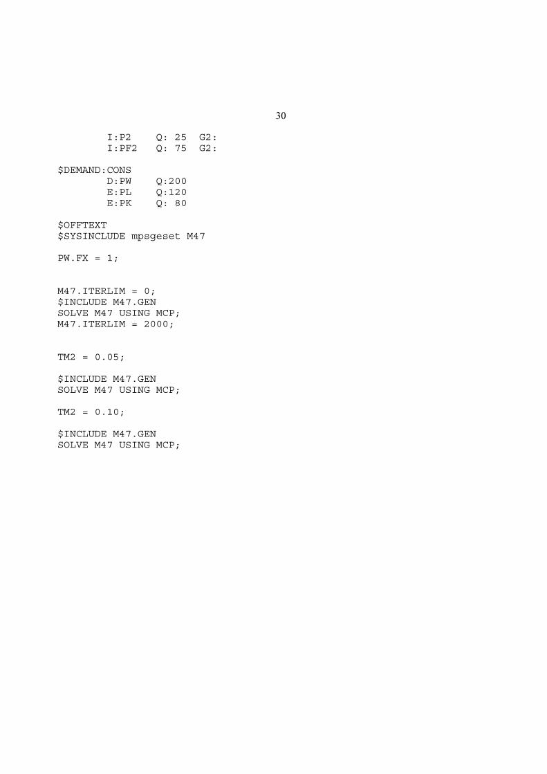
30

I:P2 Q: 25 G2: I:PF2 Q: 75 G2:



PW.FX = 1;


TM2 = 0.05;


TM2 = 0.10;


31

Model 48

For many countries, or for a small number of commodities for one country, the small-

country assumption of fixed world prices may not be appropriate. One alternative is of course to

model the whole world. But it may be convenient and appropriate for the modeler to stick with

the country and question and continue to represent the rest of the world with trade transformation

functions. The purpose of this model is to show how to do this, allowing for prices to change

with quantities supplied and demanded.

The powerful features of MPS/GE come with a few costs. One is that production blocks

(which are actually cost functions in the background) must be specified with constant returns to

scale. Yet having one fixed factor can allow output as a function of one or more variable factors

to mimic decreasing returns as we showed in model M25. We will show how to incorporate

increasing returns to scale in the next chapter.

We will use a specific factor trick to make the foreign exchange received for exports of

X1 a strictly concave function of export volume. We will create a ficticious factor called R (price

PR) which is a second input into the export function. This factor is owned by a foreign consumer

called CONSF and this consumer demands foreign exchange (price PFX). In the benchmarking

procedure, we scale up the output of export activity E1 so that when the ficticious factor is paid

the value of its marginal product, the same amount of foreign exchange is left for the domestic

economy as in the original small-economy benchmarking. Here is the data matrix, which is just a

revision of M41, adding the ficticious factor and scaling up the output of E1 to pay for the factor.


Markets | X1 X2 E1 M2 W CONSH CONSF----------------------------------------------------------------P1 | 150 -50 -100P2 | 50 50 -100PL | -100 -20 120PK | -50 -30 80PW | 200 -200PFX | 100 -50 -50PR | -50 50----------------------------------------------------------------

Consumer CONSF owns the ficticious factor (price PR) but the amount of foreign exchange left

over from exports of good 1, equal to 50, leaves 50 units of FX for the domestic consumer. Here

is the production block for activity E1.

$PROD:E1 s:1 O:PFX Q:100 I:P1 Q: 50 I:PR Q: 50

32

We have specified this as a Cobb-Douglas function, so we are assuming that it is of the

form:

FX X0.5

1 R 0.5X

1

FX

FX

X1

0.5

The elasticity of foreign exchange revenues with respect to export quantity is 0.5. Think of FX

as revenue: FX = p1(X1)X1. Then if you do the algebra, you get:

FX

X1

p1

X1

dp1

dX1

X1

FX

dFX

dX1

1X

1

p1

dp1

dX1

11

where is the elasticity of demand. If the elasticity of foreign exchange with respect to export

quantity is 0.5, then we are implicitly calibrating the elasticity of foreign demand for our exports

to be - 2. Notice that an infinite elasticity of demand for our exports means that the elasticity of

foreign exchange with respect to export quantity is 1, the small country assumption.

Note that by choosing the share parameter on the Cobb-Douglas function E1, we can

calibrate to any foreign elasticity of export demand that we like. This is done by varying the

amount of R relative to X1 in the benchmarking, remembering to scale output so that there is

always 50 units left over for the domestic consumer.

Now run the model. For a counterfactual, we have imposed an import tariff of 0.20.

Note from the listing file that this increases welfare in the domestic economy. This is the usual

“optimal tariff” argument for a large economy.

33

$TITLE Model M48: Large open economy model: large open economy

$ONTEXT


Markets | X1 X2 E1 M2 W CONSH CONSF----------------------------------------------------------------P1 | 150 -50 -100P2 | 50 50 -100PL | -100 -20 120PK | -50 -30 80PW | 200 -200PFX | 100 -50 -50PR | -50 50----------------------------------------------------------------

$OFFTEXT

PARAMETER TM2 Import tariff for good;

TM2 = 0;

$ONTEXT

$MODEL:M48

$SECTORS: X1 ! Production index for good 1 X2 ! Production index good 2 E1 ! Export index of good 1 E2 ! Export index of good 2 M1 ! Import level of good 1 M2 ! Import level of good 2 W ! Welfare index

$COMMODITIES: P1 ! Price index for good 1 P2 ! Price index for good 1 PFX ! Read exchange rate index PW ! Welfare price index PL ! Wage index PK ! Capital rental index PR ! Rent which generates the export demand function

$CONSUMERS: CONSH ! Income level for representative home agent

34

CONSF ! Income level for representative foreign agent



$PROD:E1 s:1 O:PFX Q:100 I:P1 Q: 50 I:PR Q: 50

$PROD:M2 O:P2 Q:50 I:PFX Q:50 A:CONSH T:TM2

$PROD:E2 O:PFX Q:(50*0.99) I:P2 Q:50

$PROD:M1 O:P1 Q:50 I:PFX Q:(100*1.01)


$DEMAND:CONSH D:PW Q:200 E:PL Q:120 E:PK Q: 80

$DEMAND:CONSF D:PFX Q:50 E:PR Q:50


E2.L = 0;M1.L = 0;

35


* Apply a tariff which improves the terms of trade and home* welfare:

TM2 = 0.05;


Exercises:

(1) Compute the relationship between welfare and tariff rate for different benchmark export

demand functions, where the value share of PR in E1 takes on values 0.25 and 0.75. Do

this by changing the amount of R in the benchmark, remembering to change output

accordingly to leave the return to the domestic consumer equal to 50.

(2) Replace the tariff on good 2 imports with a tax on good 1 exports, and show that you can

obtain identical equilibrium values (i.e., demonstrate Lerner symmetry).

36

Model M39

In some cases, the modeler wants to have a “world” model, or at least a full two-country

general-equilibrium model. That is what we present here. It is a textbook, 2x2x2 Heckscher-

Ohlin model: two counties, two goods, two factors. The X and Y goods, as they are labeled here,

are identical across countries. The factors are labor (L) and capital (K), and the countries are

called H (home) and F (foreign).

You now have most of the building blocks necessary for some quite complicated and

realistic models. In the present case, there is really nothing new, we are just increasing the

dimensions of the problems. Here are the data:

XHH YHH XHF YHF XFF YFF XFH YFH WH WF CONSH CONSF

PXH 150 -50 -100 PYH 50 50 -100PXF 50 50 -100PYF 150 -50 -100PWH 200 -200PWF 200 -200PLH -120 -10 130PKH -30 -40 70PLF -40 -30 70PKF -10 -120 130

The notation here for the production activities is (industry or good)(country of

production)(country of sale). Thus YFH, for example, is good Y produced in country F and sold

in country H (exported to country H). The notation for markets and prices should be fairly

obvious: PXF for example is the price of good X in country F.

There is free trade, and so there is factor-price equalization. All prices can be set to one.

Country H is labor abundant and good X is labor intensive. Country F is capital abundant and

good Y is capital intensive.

In our counterfactual experiments, we first allow country H to impose a tariff of 25% and

then both countries impose symmetric tariffs of 25%.

37

$TITLE: Model M49: 2X2X2 HECKSCHER-OHLIN MODEL* This is a full two-country HO model

$ONTEXT

XHH YHH XHF YHF XFF YFF XFH YFH WH WF CONSH CONSF

PXH 150 -50 -100 PYH 50 50 -100PXF 50 50 -100PYF 150 -50 -100PWH 200 -200PWF 200 -200PLH -120 -10 130PKH -30 -40 70PLF -40 -30 70PKF -10 -120 130

$OFFTEXT

PARAMETERS TARH TARF;

TARH = 0;TARF = 0;

$ONTEXT

$MODEL:M49

$SECTORS: WH WF XHH YHH XHF YHF XFF YFF XFH YFH

$COMMODITIES: PWH PWF PXH PXF

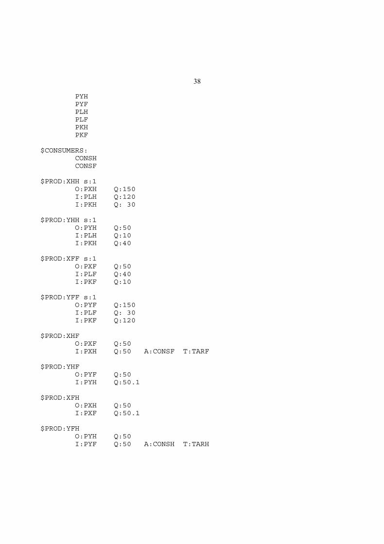
38

PYH PYF PLH PLF PKH PKF

$CONSUMERS: CONSH CONSF

$PROD:XHH s:1 O:PXH Q:150 I:PLH Q:120 I:PKH Q: 30

$PROD:YHH s:1 O:PYH Q:50 I:PLH Q:10 I:PKH Q:40

$PROD:XFF s:1 O:PXF Q:50 I:PLF Q:40 I:PKF Q:10

$PROD:YFF s:1 O:PYF Q:150 I:PLF Q: 30 I:PKF Q:120

$PROD:XHF O:PXF Q:50 I:PXH Q:50 A:CONSF T:TARF

$PROD:YHF O:PYF Q:50 I:PYH Q:50.1

$PROD:XFH O:PXH Q:50 I:PXF Q:50.1

$PROD:YFH O:PYH Q:50 I:PYF Q:50 A:CONSH T:TARH

39

$PROD:WH s:1 O:PWH Q:200 I:PXH Q:100 I:PYH Q:100

$PROD:WF s:1 O:PWF Q:200 I:PXF Q:100 I:PYF Q:100

$DEMAND:CONSH D:PWH Q:200 E:PLH Q:130 E:PKH Q: 70

$DEMAND:CONSF D:PWF Q:200 E:PLF Q: 70 E:PKF Q:130


YHF.L = 0.; XFH.L = 0.;


* TARIFFS

TARH = .25;


TARH = .25;TARF = .25;


Exercise:

Verify the Stolper-Samuelson theorem by comparing factor prices in free trade versus

when one or both countries have tariffs.

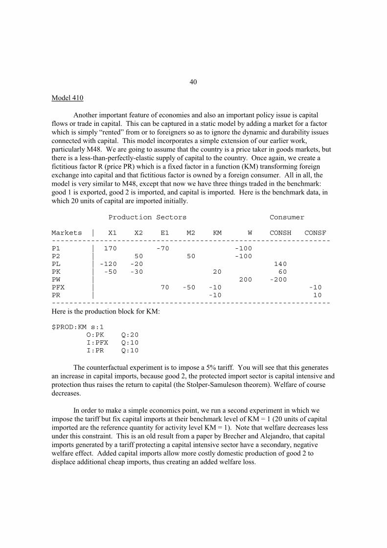
40

Model 410

Another important feature of economies and also an important policy issue is capital

flows or trade in capital. This can be captured in a static model by adding a market for a factor

which is simply “rented” from or to foreigners so as to ignore the dynamic and durability issues

connected with capital. This model incorporates a simple extension of our earlier work,

particularly M48. We are going to assume that the country is a price taker in goods markets, but

there is a less-than-perfectly-elastic supply of capital to the country. Once again, we create a

fictitious factor R (price PR) which is a fixed factor in a function (KM) transforming foreign

exchange into capital and that fictitious factor is owned by a foreign consumer. All in all, the

model is very similar to M48, except that now we have three things traded in the benchmark:

good 1 is exported, good 2 is imported, and capital is imported. Here is the benchmark data, in

which 20 units of capital are imported initially.


Markets | X1 X2 E1 M2 KM W CONSH CONSF----------------------------------------------------------------P1 | 170 -70 -100P2 | 50 50 -100PL | -120 -20 140PK | -50 -30 20 60PW | 200 -200PFX | 70 -50 -10 -10PR | -10 10----------------------------------------------------------------Here is the production block for KM:

$PROD:KM s:1 O:PK Q:20 I:PFX Q:10 I:PR Q:10

The counterfactual experiment is to impose a 5% tariff. You will see that this generates

an increase in capital imports, because good 2, the protected import sector is capital intensive and

protection thus raises the return to capital (the Stolper-Samuleson theorem). Welfare of course

decreases.

In order to make a simple economics point, we run a second experiment in which we

impose the tariff but fix capital imports at their benchmark level of KM = 1 (20 units of capital

imported are the reference quantity for activity level KM = 1). Note that welfare decreases less

under this constraint. This is an old result from a paper by Brecher and Alejandro, that capital

imports generated by a tariff protecting a capital intensive sector have a secondary, negative

welfare effect. Added capital imports allow more costly domestic production of good 2 to

displace additional cheap imports, thus creating an added welfare loss.

41

$TITLE Model M410: Capital imports (less than perfect elastic)

$ONTEXT


Markets | X1 X2 E1 M2 KM W CONSH CONSF----------------------------------------------------------------P1 | 170 -70 -100P2 | 50 50 -100PL | -120 -20 140PK | -50 -30 20 60PW | 200 -200PFX | 70 -50 -10 -10PR | -10 10----------------------------------------------------------------

$OFFTEXT

PARAMETER TM2 Import tariff for good X2;

TM2 = 0;

$ONTEXT

$MODEL:M410

$SECTORS: X1 ! Production index for good 1 X2 ! Production index good 2 E1 ! Export index of good 1 E2 ! Export index of good 2 M1 ! Import level of good 1 M2 ! Import level of good 2 KM ! Capital imports W ! Welfare index

$COMMODITIES: P1 ! Price index for good 1 P2 ! Price index for good 1 PFX ! Read exchange rate index PW ! Welfare price index PL ! Wage index PK ! Capital rental index PR ! Rent which generates concavity in capital supply

$CONSUMERS:

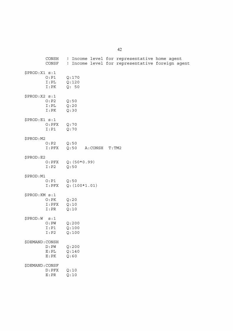
42

CONSH ! Income level for representative home agent CONSF ! Income level for representative foreign agent



$PROD:E1 s:1 O:PFX Q:70 I:P1 Q:70

$PROD:M2 O:P2 Q:50 I:PFX Q:50 A:CONSH T:TM2

$PROD:E2 O:PFX Q:(50*0.99) I:P2 Q:50

$PROD:M1 O:P1 Q:50 I:PFX Q:(100*1.01)

$PROD:KM s:1 O:PK Q:20 I:PFX Q:10 I:PR Q:10


$DEMAND:CONSH D:PW Q:200 E:PL Q:140 E:PK Q:60

$DEMAND:CONSF D:PFX Q:10 E:PR Q:10

43


E2.L = 0;M1.L = 0;

PW.FX = 1;


TM2 = 0.05;


KM.FX = 1;


1

Chapter 5

Monopoly, Oligopoly and Increasing Returns

Now we turn to models involving imperfect competition and increasing returns to scale.

These topics have attracted considerable attention in both theoretical and empirical analyses of

international trade and public economics over the last two decades. Imperfect competition

models, at least general-equilibrium models used in international trade and in public economics

often fall into one of two cases. First, there are oligopoly models with small numbers of firms

strategically interacting with one another. These models often assume that an industry produces

a homogeneous good. Second, there are monopolistic-competition models with large numbers of

firms producing differentiated goods. Individual firms are small relative to the market, which

results in greatly simplified marginal revenue functions or market rules.

Similarly, there are several classes of scale economies. An older literature in

international trade assumes that scale economies are external to individual firms but internal to

industries. This has some appeal empirically, but has some significant analytical advantages in

general-equilibrium models in that competitive pricing rules can be used. A newer literature

assumes that scale economies are internal to individual firms so that imperfect competition is an

inevitable part of the equilibrium analysis.

In this chapter we will consider monopoly/oligopoly models where markups are

endogenous and the industry output is a homogeneous good. In chapter 6, we will consider

external economies and monopolistic-competition models, which have more in common with

one another than many researchers appreciate.

Because these models have features rather different from the more standard competitive

general-equilibrium models, I will present both MCP and MPS/GE versions of each model so

that the reader can see exactly what is solved for in the MPS/GE versions. The models in this

chapter are as follows:

M51-MCP.GMS Closed economy model with monopoly in the X sector, MCP version

M51-MPS.GMS Closed economy model with monopoly in the X sector, MPS/GE version

M52-MCP.GMS Closed economy model with monopoly and increasing returns in the X

sector, MCP version.

M52-MPS.GMS Closed economy model with monopoly and increasing returns in the X

sector, MPS/GE version.

2

M53-MCP.GMS Closed economy model with monopoly, increasing returns and free

entry/exit in the X sector, MCP version

M53-MPS.GMS Closed economy model with monopoly, increasing returns and free

entry/exit in the X sector, MPS/GE version

M54-MCP.GMS Two country trade model with monopoly, increasing returns and free

entry/exit in the X sector, MCP version

M54-MPS.GMS Two country trade model with monopoly, increasing returns and free

entry/exit in the X sector, MPS/GE version

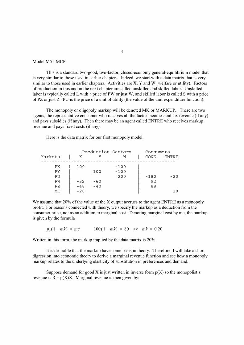
3

Model M51-MCP

This is a standard two-good, two-factor, closed-economy general-equilibrium model that

is very similar to those used in earlier chapters. Indeed, we start with a data matrix that is very

similar to those used in earlier chapters. Activities are X, Y and W (welfare or utility). Factors

of production in this and in the next chapter are called unskilled and skilled labor. Unskilled

labor is typically called L with a price of PW or just W, and skilled labor is called S with a price

of PZ or just Z. PU is the price of a unit of utility (the value of the unit expenditure function).

The monopoly or oligopoly markup will be denoted MK or MARKUP. There are two

agents, the representative consumer who receives all the factor incomes and tax revenue (if any)

and pays subsidies (if any). Then there may be an agent called ENTRE who receives markup

revenue and pays fixed costs (if any).

Here is the data matrix for our first monopoly model.

Production Sectors Consumers Markets | X Y W | CONS ENTRE ------------------------------------------------- PX ! 100 -100 | PY | 100 -100 | PU | 200 | -180 -20 PW | -32 -60 | 92 PZ | -48 -40 | 88 MK | -20 | 20

We assume that 20% of the value of the X output accrues to the agent ENTRE as a monopoly

profit. For reasons connected with theory, we specify the markup as a deduction from the

consumer price, not as an addition to marginal cost. Denoting marginal cost by mc, the markup

is given by the formula

px(1 mk ) mc 100(1 mk ) 80 > mk 0.20

Written in this form, the markup implied by the data matrix is 20%.

It is desirable that the markup have some basis in theory. Therefore, I will take a short

digression into economic theory to derive a marginal revenue function and see how a monopoly

markup relates to the underlying elasticity of substitution in preferences and demand.

Suppose demand for good X is just written in inverse form p(X) so the monopolist’s

revenue is R = p(X)X. Marginal revenue is then given by:

4

(1)

R

Xp X

p

Xp p

X

p

p

Xp 1

1MR

MR p (1 mk ) mk1 p

X

X

p

where η is the Marshallian elasticity of demand, defined as positive. The monopoly markup is

just the inverse of this elasticity. This looks good, but what is η in general equilibrium?

Suppose now that there are two goods, X1 and X2, and consumer income is given by M. I

will assume a symmetric CES utility function and assure the reader that the formula I derive is

applicable to a more general case with different weights on the goods. The utility function is

given as follows, where σ is the elasticity of substitution between goods. For a monopoly

equilibrium to exist, we must have σ > 1, which in turn imposes the restriction that 1 > α > 0.

(2) U X1 X2

1

Maximizing utility subject to the usual linear budget constraint, yields demand functions:

(3) Xi

pi p1

j

1M

1

1,

1

Taking the own-derivative, we have:

(4)Xi

pi

p1

i p1

j

1M pi p

1

j

2( 1)pi M

Forming the elasticity, we get:

(5)pi

Xi

Xi

pi

( 1)p1

i p1

j

1si

piXi

Mp

1

i p1

j

1

The second equation gives the share of income spent on good i, si, by multiplying through (3) by

5

pi and dividing both sides by M. We see that this share appears in the second term of the first

equation. Thus the elasticity of demand for Xi can be written as:

(6)i

pi

Xi

Xi

pi

( 1)si

mk ( 1)si

1

Note that Cobb-Douglas, σ = 1, is a special case in which the Marshallian elasticity is also equal

to 1.

Now we are able to calibrate our data to an underlying theory. That is, we assume that

this data is generated by a standard monopoly pricing model and that preferences are CES. The

data show that the share of expenditure on X is 0.50, and the markup is 0.20, so η = 5. Solving

for the implied elasticity of substitution in preferences, we get σ = 9. We will use this value in

the data to follow.

The final issue is also one of calibration. If we let the marginal cost (or producer price) of

X = 1, then the markup implies that the consumer price is px = 1.25. Suppose that we wish to

chose units so that all other prices are equal to one, a convention that we like to adopt. The cost

function for utility (utility price = pu) which is dual to the utility function given above is given

by:

(7) pu p1

x p1

y

1

1

In our case, the price of good X is 1.25, so we can divide px in this cost function to calibrated

initially so that both additive terms in the function equal 1. But then the term in square brackets

equals 2, so if we want pu = 1 initially we have to compensate with a multiplicative constant on

the front of the function. Denote this term as A. The calibrated cost function for utility is then:

A*((PX/1.25)**(1-SIGMA) + PY**(1-SIGMA))**(1/(1-SIGMA)) =G= PU;

A = 0.5**(1/(1-SIGMA))

This is satisfied with equality at px = 1.25, py = 1, and pu = 1. The parameter A will then also

appear in the demand functions for X and Y, which are derived from Shepard’s lemma. The

demand for X, for example, is the derivative of (7) with respect to px, times the level of welfare.

Initial X output is X*80 (i.e., the activity level X is set at one, where X =1 generates 80 units of

output) and initial welfare is similarly W*200. Thus the demand for X is given by;

6

X*80 =E= A*(PX/1.25)**(-SIGMA)*((PX/1.25)**(1-SIGMA) + PY**(1-SIGMA))**(SIGMA/(1-SIGMA)) *W*200/1.25;

Now you might see why I like MPS/GE (and this is a pretty simple case). The latter will

automatically calculate scaling coefficients like A from the data provided in a production block,

and then automatically apply Shepard’s lemma to get commodity and factor demands.

The rest of the program should be fairly transparent at this point. Two equations are

added to calculate the share of expenditure on X (SHX) and the markup (MK). The agent

ENTRE receives income from markups and demands utility just like the representative agent.

After the model solves, we calculate how total income is divided between the representative

factor owner (INCOMEC) and the monopolist (INCOMEM).

The counter-factual experiment is to impose marginal-cost pricing, which we can do by

simply fixing the markup at zero with the statement MARKUP.FX = 0. Not only does welfare

increase, but factor owners have a much bigger proportional increase since there is also a

redistribution from monopoly profits to the factor owners. Overall welfare rises by 4% following

the imposition of marginal-cost pricing, so this is a measure of deadweight loss from monopoly.

But consumer (factor owner) welfare rises by 15.6% (0.90 to 1.04) which is much more

significant.

7

$TITLE Model M51-MCP.GMS: Closed 2x2 Economy, monopoly X producer* MCP version

$ONTEXT


$Offtext

PARAMETERSA Scale parameter for utility function,SIGMA Elasticity of substitution,INCOMEM Monopoly profit (in welfare units),INCOMEC factor owners' income,ENDOWSENDOWLMODELSTAT;

SIGMA = 9;ENDOWS = 88;ENDOWL = 92;A = 0.5**(1/(1-SIGMA));

POSITIVE VARIABLESXYWPXPYPUPZPWCONSENTRESHAREXMARKUP;

8

EQUATIONSDX Demand for XDY Demand for YDW Demand for WPRICEX MR = MC in XPRICEY Zero profit condition for Y (PY = MC)PRICEW Zero profit condition for WSKLAB Supply-demand balance for skilled laborUNLAB Supply-demand balance for unskilled laborICONS Consumer (factor owners') incomeIENTRE Entrepreneur's profitsSHX Share of X in expenditureMK Markup equation;

PRICEX.. (PW**0.40)*(PZ**0.60) =G= PX*(1 - MARKUP);

PRICEY.. (PW**0.60)*(PZ**0.40) =G= PY;

PRICEW.. A*((PX/1.25)**(1-SIGMA) + PY**(1-SIGMA))**(1/(1-SIGMA)) =G= PU;

DX.. X*80 =E= A*(PX/1.25)**(-SIGMA)* ((PX/1.25)**(1-SIGMA) + PY**(1-SIGMA))**(SIGMA/(1-SIGMA)) *W*200/1.25;

DY.. Y*100 =E= A*PY**(-SIGMA)* ((PX/1.25)**(1-SIGMA) + PY**(1-SIGMA))**(SIGMA/(1-SIGMA)) *W*200;

DW.. W*200 =E= (CONS + ENTRE)/PU;

SKLAB.. ENDOWS =E= 0.40*(PW**0.60)*(PZ**(0.40-1))*Y*100 + 0.60*(PW**0.40)*(PZ**(0.60-1))*X*80;

UNLAB.. ENDOWL =E= 0.60*(PW**(0.60-1))*(PZ**0.40)*Y*100 + 0.40*(PW**(0.40-1))*(PZ**0.60)*X*80;

ICONS.. CONS =E= PZ*ENDOWS + PW*ENDOWL;

IENTRE.. ENTRE =E= MARKUP*PX*X*80;

SHX.. SHAREX =E= 80*PX*X / (80*PX*X + 100*PY*Y) ;

MK.. MARKUP =E= 1/(SIGMA - (SIGMA-1)*SHAREX);

9

MODEL M51 /DX.PX, DY.PY, DW.PU, PRICEX.X, PRICEY.Y, PRICEW.W, SKLAB.PZ, UNLAB.PW, ICONS.CONS, IENTRE.ENTRE SHX.SHAREX, MK.MARKUP/;

OPTION MCP=MILES;OPTION LIMROW=0;OPTION LIMCOL=0;$OFFSYMLIST OFFSYMXREF OFFUELLIST OFFUELXREF

CONS.L = 200;X.L = 1;Y.L = 1;W.L = 1;PX.L = 1.25;PY.L = 1;PZ.L = 1;PW.L = 1;PU.L = 1;CONS.L = 180;ENTRE.L = 20;SHAREX.L = 0.5;MARKUP.L = 0.20;

PY.FX = 1;

*M51.ITERLIM = 0;SOLVE M51 USING MCP;MODELSTAT = M51.MODELSTAT - 1.;

INCOMEM = W.L*(ENTRE.L/(ENTRE.L + CONS.L));INCOMEC = W.L*(CONS.L/(ENTRE.L + CONS.L));

DISPLAY INCOMEM, INCOMEC;

* Evaluate the potential gains from first-best (marginal* cost) pricing:

MARKUP.FX = 0;

SOLVE M51 USING MCP;



10

Model M51-MPS

This model is identical to the previous model, except that this one is coded in MPS/GE.

There is not a lot that needs to be said here. The basic simplifying trick is to use the “N” field in

a production block to denote an endogenous “tax rate”, which is in this case the markup. The

revenue from this tax is assigned to the agent ENTRE as monopoly profits. The endogenous tax

rate is an auxiliary variable which is then set in a constraint equation. The production block is

given by:

$PROD:X s:1 O:PX Q: 80 A:ENTRE N:MARKUP I:PW Q: 32 I:PZ Q: 48

Note that if we use the formula derived above, we want the tax set on the output so that we

indeed have PX(1 - MARKUP) = MC. If the tax was set on the two input fields, we would have

PX = (1+MARKUP)MC. The same markup does not yield the same relationship between price

and marginal cost in the two cases since the tax base is different in the two situations. So be

careful to specify the production block carefully.

Second, remember to include the price field in the production block for welfare in order

for MPS/GE to correctly calibrate the function. This is given by:

$PROD:W s:SIGMA O:PU Q:200 I:PX Q:80 P:1.25 I:PY Q:100

It should be clear that MPS/GE is going to do a lot of work for you, but you must give it the

correct information to get a correct calibration.

The endogenous markup is set using two auxiliary variables and two constraint equations.

$CONSTRAINT:SHAREX SHAREX =E= 80*PX*X / (80*PX*X + 100*PY*Y) ;

$CONSTRAINT:MARKUP MARKUP =E= 1/(SIGMA - (SIGMA-1)*SHAREX);

The rest of the coding should be clear at this point.

11

$TITLE Model M51-MPS.GMS: Closed 2x2 Economy, monopoly X producer* MPS/GE version

$ONTEXT


$offtext

SCALAR SIGMA Elasticity of substitution, INCOMEM Monopoly profit (in welfare units), INCOMEC factor owners' income;

SIGMA = 9;

$ONTEXT

$MODEL:M51


$COMMODITIES: PX ! Price index for commodity X PY ! Price index for commodity Y PW ! Price index for primary factor L (net of tax) PZ ! Price index for primary factor K PU ! Price index for welfare (expenditure function)

$CONSUMERS: CONS ! Representative agent. ENTRE ! Entreprenuer (monopolist)

$AUXILIARY: SHAREX ! Value share of good X MARKUP ! X sector markup on marginal cost

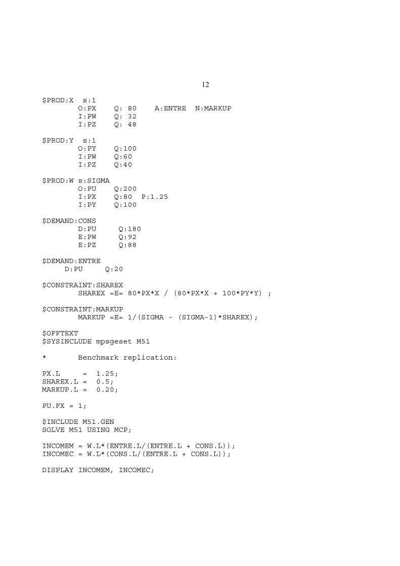
12


$PROD:Y s:1 O:PY Q:100 I:PW Q:60 I:PZ Q:40

$PROD:W s:SIGMA O:PU Q:200 I:PX Q:80 P:1.25 I:PY Q:100

$DEMAND:CONS D:PU Q:180 E:PW Q:92 E:PZ Q:88

$DEMAND:ENTRED:PU Q:20

$CONSTRAINT:SHAREX SHAREX =E= 80*PX*X / (80*PX*X + 100*PY*Y) ;




PX.L = 1.25;SHAREX.L = 0.5;MARKUP.L = 0.20;

PU.FX = 1;




13

* Evaluate the potential gains from first-best (marginal* cost) pricing:

MARKUP.FX = 0;




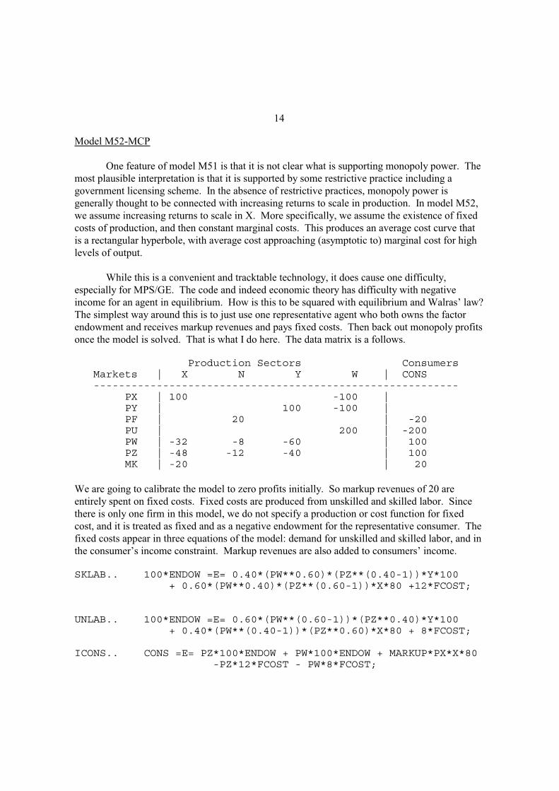
14

Model M52-MCP

One feature of model M51 is that it is not clear what is supporting monopoly power. The

most plausible interpretation is that it is supported by some restrictive practice including a

government licensing scheme. In the absence of restrictive practices, monopoly power is

generally thought to be connected with increasing returns to scale in production. In model M52,

we assume increasing returns to scale in X. More specifically, we assume the existence of fixed

costs of production, and then constant marginal costs. This produces an average cost curve that

is a rectangular hyperbole, with average cost approaching (asymptotic to) marginal cost for high

levels of output.

While this is a convenient and tracktable technology, it does cause one difficulty,

especially for MPS/GE. The code and indeed economic theory has difficulty with negative

income for an agent in equilibrium. How is this to be squared with equilibrium and Walras’ law?

The simplest way around this is to just use one representative agent who both owns the factor

endowment and receives markup revenues and pays fixed costs. Then back out monopoly profits

once the model is solved. That is what I do here. The data matrix is a follows.

Production Sectors Consumers Markets | X N Y W | CONS ---------------------------------------------------------- PX | 100 -100 | PY | 100 -100 | PF | 20 | -20 PU | 200 | -200 PW | -32 -8 -60 | 100 PZ | -48 -12 -40 | 100 MK | -20 | 20

We are going to calibrate the model to zero profits initially. So markup revenues of 20 are

entirely spent on fixed costs. Fixed costs are produced from unskilled and skilled labor. Since

there is only one firm in this model, we do not specify a production or cost function for fixed

cost, and it is treated as fixed and as a negative endowment for the representative consumer. The

fixed costs appear in three equations of the model: demand for unskilled and skilled labor, and in

the consumer’s income constraint. Markup revenues are also added to consumers’ income.

SKLAB.. 100*ENDOW =E= 0.40*(PW**0.60)*(PZ**(0.40-1))*Y*100 + 0.60*(PW**0.40)*(PZ**(0.60-1))*X*80 +12*FCOST;

UNLAB.. 100*ENDOW =E= 0.60*(PW**(0.60-1))*(PZ**0.40)*Y*100 + 0.40*(PW**(0.40-1))*(PZ**0.60)*X*80 + 8*FCOST;

ICONS.. CONS =E= PZ*100*ENDOW + PW*100*ENDOW + MARKUP*PX*X*80 -PZ*12*FCOST - PW*8*FCOST;

15

After solving the model, we recover monopoly profits. I specify this in welfare units,

multiplying welfare (syntax W.L since we have already solved the model - recall that this is the

way to report the value of a variable in an MCP or MPS/GE program). I multiply this by the

ratio of the monopolist’s profits, markup revenues minus fixed costs, to the total value of output.

So the parameter INCOMEM gives the share of welfare that is monopoly profits. INCOMEC

gives the income of consumers (factor owners).

INCOMEM = W.L*((MARKUP.L*PX.L*X.L*80 - PW.L*8*FCOST - PZ.L*12*FCOST)/(PX.L*X.L*80 + PY.L*Y.L*100));

INCOMEC = W.L - INCOMEM;


The first counter-factual imposes marginal-cost pricing by setting the markup equal to

zero (MARKUP.FX = 0). Welfare increases by 4% as in our previous example, but factor

owners have a much bigger increase, assuming that they do not have to pay the deficit (an

unrealistic assumption).

The second and third counterfactuals allow monopoly pricing and change the size of the

economy. The correct syntax for re-freeing up the markup is to set upper and lower for the

variable.

MARKUP.LO = -INF;MARKUP.UP = INF;

Making the economy larger generates positive monopoly profits and making the economy

smaller generates losses, even at the optimal markup. Thus we have a “natural monopoly” in this

model. Note the influence of increasing returns in the experiment where we make the economy

bigger. Real income and welfare increase more than in proportion to the size of the endowment.

Welfare rises from 1.0 to 2.113; however, all of the increase goes to the monopolist and the

welfare “per capita” of factor owners is virtually unchanged at 1.998 after doubling the

endowment.

16

$TITLE Model M52-MCP.GMS: Closed Economy Monopoly with IRS* uses MCP

$ONTEXT


$OFFTEXT

PARAMETERSA Scale parameter for utility function,SIGMA Elasticity of substitution,INCOMEM Monopoly profit (in welfare units),INCOMEC Factor owners' income,ENDOW Endowment scale multiplier,FCOST Fixed costs scale multiplier,MODELSTAT;

SIGMA = 9;ENDOW = 1;FCOST = 1;

A = 0.5**(1/(1-SIGMA));

POSITIVE VARIABLESXYWPXPYPUPZPWCONSENTRESHAREXMARKUP;

17

EQUATIONSDX Demand for XDY Demand for YDW Demand for WPRICEX MR = MC in XPRICEY Zero profit condition for Y (PY = MC)PRICEW Zero profit condition for WSKLAB Supply-demand balance for skilled laborUNLAB Supply-demand balance for unskilled laborICONS Consumer (factor owners') incomeIENTRE Entrepreneur's profitsSHX Share of X in expenditureMK Markup equation;


PRICEY.. (PW**0.60)*(PZ**0.40) =G= PY;

PRICEW.. A*((PX/1.25)**(1-SIGMA) + PY**(1-SIGMA))**(1/(1-SIGMA)) =G= PU;

DX.. X*80 =E= A*(PX/1.25)**(-SIGMA)* ((PX/1.25)**(1-SIGMA) + PY**(1-SIGMA))**(SIGMA/(1-SIGMA)) *W*200/1.25;

DY.. Y*100 =E= A*PY**(-SIGMA)* ((PX/1.25)**(1-SIGMA) + PY**(1-SIGMA))**(SIGMA/(1-SIGMA)) *W*200;

DW.. W*200 =E= CONS/PU;

SKLAB.. 100*ENDOW =E= 0.40*(PW**0.60)*(PZ**(0.40-1))*Y*100 + 0.60*(PW**0.40)*(PZ**(0.60-1))*X*80 +12*FCOST;

UNLAB.. 100*ENDOW =E= 0.60*(PW**(0.60-1))*(PZ**0.40)*Y*100 + 0.40*(PW**(0.40-1))*(PZ**0.60)*X*80 + 8*FCOST;

ICONS.. CONS =E= PZ*100*ENDOW + PW*100*ENDOW + MARKUP*PX*X*80 -PZ*12*FCOST - PW*8*FCOST;

SHX.. SHAREX =E= 80*PX*X / (80*PX*X + 100*PY*Y) ;

MK.. MARKUP =E= 1/(SIGMA - (SIGMA-1)*SHAREX);

18

MODEL M52 /DX.PX, DY.PY, DW.PU, PRICEX.X, PRICEY.Y, PRICEW.W, SKLAB.PZ, UNLAB.PW, ICONS.CONS, SHX.SHAREX, MK.MARKUP/;


CONS.L = 200;X.L = 1;Y.L = 1;W.L = 1;PX.L = 1.25;PY.L = 1;PZ.L = 1;PW.L = 1;PU.L = 1;CONS.L = 180;ENTRE.L = 20;SHAREX.L = 0.5;MARKUP.L = 0.20;

PY.FX = 1;


INCOMEM = W.L*((MARKUP.L*PX.L*X.L*80 - PW.L*8*FCOST - PZ.L*12*FCOST)/ (PX.L*X.L*80 + PY.L*Y.L*100));INCOMEC = W.L - INCOMEM;


* counterfactual: marginal-cost pricing

MARKUP.FX = 0;




19

* counterfactual: double the size of the economy


ENDOW = 2;




* counterfactual: cut the size of the economy by 25%

ENDOW = 0.75;




20

Model M52-MPS

This model is quite similar to model M51, so there is not a lot to add concerning the

MPS/GE version of model M52. The one thing worth noting is how the fixed costs are modeled

here. These are specified as negative endowments in the consumer demand block. This is a

good time to give a reminder that when a Q, P, or E field specifies an arithmetic operation the

expression must be in parentheses. So an expression such as “Q: 100*ENDOW” is not allowed.

$DEMAND:CONS D:PU Q:200 E:PW Q:(100*ENDOW) E:PZ Q:(100*ENDOW) E:PW Q:(-8*FCOST) E:PZ Q:(-12*FCOST)

This formulation allows fixed costs and the overall endowment to be adjusted

independently. The negative endowments are not a problem unless a consumer is left with

negative income, a problem discussed earlier.

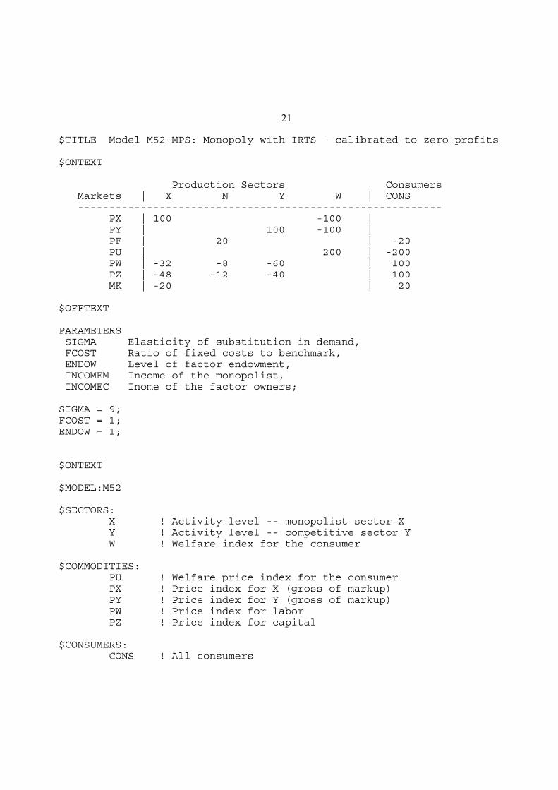
21

$TITLE Model M52-MPS: Monopoly with IRTS - calibrated to zero profits

$ONTEXT


$OFFTEXT

PARAMETERS SIGMA Elasticity of substitution in demand, FCOST Ratio of fixed costs to benchmark, ENDOW Level of factor endowment, INCOMEM Income of the monopolist, INCOMEC Inome of the factor owners;

SIGMA = 9;FCOST = 1;ENDOW = 1;

$ONTEXT

$MODEL:M52

$SECTORS: X ! Activity level -- monopolist sector X Y ! Activity level -- competitive sector Y W ! Welfare index for the consumer

$COMMODITIES: PU ! Welfare price index for the consumer PX ! Price index for X (gross of markup) PY ! Price index for Y (gross of markup) PW ! Price index for labor PZ ! Price index for capital

$CONSUMERS: CONS ! All consumers

22

$AUXILIARY: SHAREX ! Value share of X in total consumption MARKUP ! Markup based on Marshallian demand

$PROD:X s:1 O:PX Q: 80 A:CONS N:MARKUP I:PW Q: 32 I:PZ Q: 48

$PROD:Y s:1 O:PY Q:100 I:PW Q: 60 I:PZ Q: 40

$PROD:W s:sigma O:PU Q:200 I:PX Q: 80 P:1.25 I:PY Q:100

$DEMAND:CONS D:PU Q:200 E:PW Q:(100*ENDOW) E:PZ Q:(100*ENDOW) E:PW Q:(-8*FCOST) E:PZ Q:(-12*FCOST)

$CONSTRAINT:SHAREX SHAREX*(80*PX*X + 100*PY*Y) =G= 80*PX*X;




PX.L = 1.25; SHAREX.L = 0.5; MARKUP.L = 0.20;



23


* counterfactual: marginal-cost pricing

MARKUP.FX = 0;






ENDOW = 2;




* counterfactual: cut the size of the economy by 25%

ENDOW = 0.75;




24

Model M53-MCP

Cases of pure monopoly or indeed cases with any fixed number of firms are likely rare in

economics, and models allowing entry and exit as conditions change are clearly desirable. There

is however a significant technical difficulty with allowing the number of firms to change but

restricting the number to integer values. The equilibrium number of firms N is found when the N

firms make non-negative profits but N+1 firms do make loses. The zero-profit condition cannot

be specified as an equality when there are positive numbers of firms. Then the model become an

integer complementarity problem and we have no good algorithms for solving this type of

problem. The problem could be handled by brute force where there is only one type of firm by

iterating over the (integer) number of firms, but even this breaks down when there are several

possible firm types (e.g., firms from different countries, multinational versus domestic firms,

etc.).

The classic and accepted way around this difficulty is to allow the number of firms to be a

continuous variable. This is of course how monopolistic-competition models have always been

formulated. While this trick is initially hard to swallow conceptually, it has the powerful

analytical advantage of allowing us to specify the entry condition as an inequality, holding with

equality if there are a positive number of firms active in equilibrium. This is the technique we

adopt here. The data matrix for the problem is:

Production Sectors Consumers Markets | X N Y W | CONS ENTRE ---------------------------------------------------------- PX | 100 -100 | PY | 100 -100 | PF | 20 | -20 PU | 200 | -200 PW | -32 -8 -60 | 100 PZ | -48 -12 -40 | 100 MK | -20 | 20

Firm owners receive markup revenues and “demand” fixed costs. N will be an activity and in

equilibrium the activity level will be interpreted as the number of firms producing X. The model

is calibrated to zero profits initially, so the markup revenues (20) will cover fixed costs (20).

Firm “owners” are represented by the single agent ENTRE.

Here I am going to introduce a somewhat different calibration scheme than that used

above. Instead of assuming a given number of firms and using the data and markup formula to

solve for the implied elasticity of substitution in demand, I am going to assume Cobb-Douglas

preferences and solve for the implied number of firms in the benchmark equilibrium. To do this,

we need to derive the Cournot markup formula when there is more than one firm.

Revenue for a Cournot firm i is given by . The Marshallian price elasticityRi

p (Xc)X

i

25

of demand is denoted η. η is just -1 in our formulation with Cobb-Douglas demand in (6) since

here σ = 1. Cournot conjectures imply that ; that is, a one-unit increase in ownXc/ X

i1

supply is a one-unit increase in market supply. Marginal revenue is then:

MRi

Ri

Xi

p Xi

p

Xc

Xc

Xi

p pXi

Xc

Xc

p

p

Xc

Xc

Xi

p 1Xi

Xc

1

MRi

p (1 mki) mk

i

si p

Xc

Xc

p

Xi

Xc

si

The combined assumptions of Cournot pricing and Cobb-Douglas preferences lead to a very

simple expression for a firm’s markup, which is given by the firm’s market share.

mki

Xi

Xc

si

since 1 (Cobb Douglas)

In the data given above, the implied markup is 20%, thus there must be five firms active

initially given Cobb-Douglas preferences. The model below is calibrated with N = 5 initially.

We now have two additional equations and unknowns relative to the previous model. There is

the quantity (N) and unit price of fixed costs (PF) which are the complementary variables for the

zero-profit equation for fixed costs (PRICEF) and the market clearing equation for fixed costs

(DF) respectively. These are given by:

PRICEF.. (PW**0.40)*(PZ**0.60) =G= PF; (complementary to N)

DF.. N*4 =G= ENTRE/PF; (complementary to PF)

We have to remember that total fixed costs are 20 and therefore we must use N*4 (= 20)

for the demand for fixed costs for a consistent calibration at N = 5. N then appears in the markup

equation as given by the algebra above and the markup revenue in turn provides the entrepreneur

with income (ENTRE).

MK.. MARKUP*N =E= 1; (complementary to MARKUP)

IENTRE.. ENTRE =E= MARKUP*PX*X*80; (complementary to ENTRE)

Thus the entrepreneur is treated as a consumer who derives income from markup revenues with

26

that income spent on a good called fixed costs. Total fixed costs are interpreted as the number of

firms in equilibrium, which in turn feeds into the markup formula.

Alternatively, I could have chosen units to let N = 1, and then the correct quantity in the

factor-demand equations and fixed-cost pricing equations would be N*20 and the market

equation would be MARKUP*N*5 =E= 1. This latter case is convenient for the same reason that

it is always convenient to have activity levels and prices calibrated to one initially: the new

equilibrium levels in counter factual experiments are proportional changes from the benchmark.

Many calibration errors are due to inconsistent use of units and representative quantity and price

units in different functions. So it is a useful exercise here to recalibrate the model to N = 1. N

appears in four equations in the model and as just indicated, something must be changed in each

of those four equations.

The counterfactual-experiment is to double the size of the economy. Note that this more

than doubles welfare, which rises to 2.072. X production more than doubles but the number of

firms much less than doubles, rising from 5.0 to 7.071. Increases in the number of firms leads

each individual firm to perceive demand as more elastic and the equilibrium markup falls from

0.20 to 0.14. There is an increase in the output per firm, firms move down their average costs

curves and become more technically efficient.

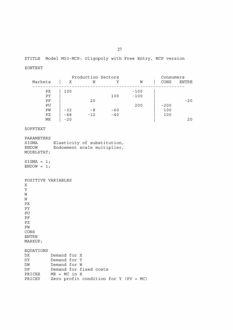
27

$TITLE Model M53-MCP: Oligopoly with Free Entry, MCP version

$ONTEXT


$OFFTEXT

PARAMETERSSIGMA Elasticity of substitution,ENDOW Endowment scale multiplier,MODELSTAT;

SIGMA = 1;ENDOW = 1;

POSITIVE VARIABLESXYWNPXPYPUPFPZPWCONSENTREMARKUP;

EQUATIONSDX Demand for XDY Demand for YDW Demand for WDF Demand for fixed costsPRICEX MR = MC in XPRICEY Zero profit condition for Y (PY = MC)

28

PRICEW Zero profit condition for WPRICEF Zero profit condition for fixed costsSKLAB Supply-demand balance for skilled laborUNLAB Supply-demand balance for unskilled laborICONS Consumer (factor owners') incomeIENTRE Entrepreneur's profitsMK Markup equation;


PRICEY.. (PW**0.60)*(PZ**0.40) =G= PY;

PRICEW.. ((PX/1.25)**0.5)*(PY**0.5) =G= PU;

PRICEF.. (PW**0.40)*(PZ**0.60) =G= PF;

DX.. X*80 =E= 0.5*CONS/PX;

DY.. Y*100 =E= 0.5*CONS/PY;

DW.. W*200 =E= CONS/PU;

DF.. N*4 =G= ENTRE/PF;

SKLAB.. 100*ENDOW =E= 0.40*(PW**0.60)*(PZ**(0.40-1))*Y*100 + 0.60*(PW**0.40)*(PZ**(0.60-1))*X*80

+ 0.60*(PW**0.40)*(PZ**(0.60-1))*N*4;

UNLAB.. 100*ENDOW =E= 0.60*(PW**(0.60-1))*(PZ**0.40)*Y*100 + 0.40*(PW**(0.40-1))*(PZ**0.60)*X*80 + 0.40*(PW**(0.40-1))*(PZ**0.60)*N*4;

ICONS.. CONS =E= PZ*100*ENDOW + PW*100*ENDOW;

IENTRE.. ENTRE =E= MARKUP*PX*X*80;

MK.. MARKUP*N =E= 1;

MODEL M53 /DX.PX, DY.PY, DW.PU, DF.PF, PRICEX.X, PRICEY.Y, PRICEW.W, PRICEF.N, SKLAB.PZ, UNLAB.PW, ICONS.CONS, IENTRE.ENTRE, MK.MARKUP/;

OPTION MCP=MILES;OPTION LIMROW=0;OPTION LIMCOL=0;

29

$OFFSYMLIST OFFSYMXREF OFFUELLIST OFFUELXREF

CONS.L = 200;X.L = 1;Y.L = 1;W.L = 1;N.L = 4;PX.L = 1.25;PY.L = 1;PZ.L = 1;PW.L = 1;PU.L = 1;PF.L = 1;CONS.L = 180;ENTRE.L = 20;MARKUP.L = 0.20;

PY.FX = 1;



ENDOW = 2;


30

Model M53-MPS

Relative to M52, we now add one activity (N) and one commodity (PF) to the model. As

in the MCP version just discussed, we need to be careful about calibration. If we choose N = 5

as the calibration, then the representative quantities for the $PROD:N block are the total

quantities from the data matrix divided by 5, and the markup equation just uses N.

$PROD:N s:1 O:PF Q: (20/5) I:PW Q: (8/5) I:PZ Q: (12/5)

$CONSTRAINT:MARKUP MARKUP*N =E= 1;

If instead, we want an initial value of N = 1, then we would need

$PROD:N s:1 O:PF Q: 20 I:PW Q: 8 I:PZ Q: 12

$CONSTRAINT:MARKUP MARKUP*N*5 =E= 1;

As I have emphasized several times, MPS/GE automatically generates the appropriate

factor demand equations, and so there is no need to have to worry about consistency of units for

these equations as we have to do in the MCP version.

31

$TITLE Model M53-MPS: Oligopoly with free entry, MPS/GE version

$ONTEXT


$OFFTEXT

PARAMETERS SIGMA ENDOW;

SIGMA = 1;ENDOW = 1;

$ONTEXT

$MODEL:M53

$SECTORS: X ! Activity level - sector X output Y ! Activity level - competitive sector Y W ! Welfare index for the representative consumer N ! Activity level - sector X fixed costs = no. of firms

$COMMODITIES: PU ! Price index for representative agent utility PX ! Price of good X (gross of markup) PY ! Price of good Y PF ! Unit price of inputs to fixed cost PW ! Price index for labor PZ ! Price index for capital

$CONSUMERS: CONS ! Representative agent ENTRE ! Entrepreneur (converts markup revenue to fixed cost)

32

$AUXILIARY: MARKUP ! Optimal markup based on Marshallian demand elasticity



$PROD:N s:1 O:PF Q: (20/5) I:PW Q: (8/5) I:PZ Q: (12/5)

$PROD:W s:1 O:PU Q:200 I:PX Q: 80 P:1.25 I:PY Q:100

$DEMAND:CONS D:PU Q:200 E:PW Q:(ENDOW*100) E:PZ Q:(ENDOW*100)

$DEMAND:ENTRE D:PF Q: 20

$CONSTRAINT:MARKUP MARKUP*N =E= 1;



N.L = 5;PX.L = 1.25;MARKUP.L = 0.20;


33

* Counterfactual double the size of economy.

ENDOW = 2;


34

Model M54-MCP

Model M54 is a two-country version of M53. The initial data specifies that the countries

are identical, and trade is costless. There is really not a lot new here, except that one has to be

careful about the initial calibration of the markups. Markup revenues in the two markets are 20%

of sales and once again we will assume Cobb-Douglas preferences. Thus there are once again 5

firms in total. This is turn implies that there are 2.5 firms in each country initially. I realize that

this might be troublesome for some readers, and there are of course alternative calibrations such

as the procedure discussed earlier where we choose the number of firms and calibrate the

elasticity of substitution. Or in some cases research just use a “conjectural variation” parameter

which is a multiplicative constant on the markup to reconcile the actual markup with the one

given by the assumed number of firms. The modeler often has no alternative to this last

procedure when trying to calibrate a model to real data.

A couple of features deserve discussion. First, this is a model in which I assume that

markets are segmented, meaning that firms can price independently in the two markets (the two

prices need not differ by exactly the transport/tariff cost). In general, firms will have different

market shares and thus different markups in the two countries, and thus it is important to have

different pricing conditions for the two supplies of a given firm. Here I use a technique that is

very useful in many models, which is to add additional activities. I first have one activity that

converts factors into aggregate firm output. Then this output is the input into two separate

activities, one which supplies output to the domestic market and one which supplies the foreign

(export) market.

For country j, the PXDJ denotes the producer price, or cost of aggregate X output, XJ, so

the value of this variable is the marginal cost of production. This aggregate supply is then

divided by supply to j, XJJ, and exports to i, XJI (XJ = XJJ + XJI). Consumer price of XJ in

country j is given by PXJ and that in country i by PXI. The relationship between marginal cost

and consumer prices depends on the markups in the two markets and on transport costs on

exported output. The relevant pricing equations for firms in j, with complementary variables in

parenthesis are:

PRXDJ.. (WJ**0.40)*(ZJ**0.60) =G= PXDJ; (XJ)

PRXJJ.. PXDJ =G= PXJ*(1 - MARKJJ); (XJJ)

PRXJI.. PXDJ*(1+TC) =G= PXI*(1 - MARKJI); (XJI)

Given Cobb-Douglas preferences, a firm’s markup is just its market share. I have coded

the model such that the X variables just introduced are the total outputs of all firms located in

country j. Thus to get the output (sales) of an individual firm from j in a market, we have to

divide these quantities by the number of j firms NJ. Thus, for example, the supply of a single j

firm to market j is given by

35

(XJJ/NJ)/(XIJ + XJJ)) or XJJ/(NJ*(XIJ + XJJ));

The markup equations are thus given by:

MKII.. MARKII =E= XII/(NI*(XII + XJI));MKIJ.. MARKIJ =E= XIJ/(NI*(XIJ + XJJ));MKJJ.. MARKJJ =E= XJJ/(NJ*(XIJ + XJJ));MKJI.. MARKJI =E= XJI/(NJ*(XII + XJI));

I coded the MPS/GE version of this model first, which took very little time. Then I tried

to code this corresponding MCP. I made a few mistakes, things that MPS/GE does

automatically, and it took me quite a while. So I pass on comments about my mistakes. First,

trade costs require that more output must be shipped than is received. The relationships between

firms’ total outputs and supplies to the two markets are given by:

DXDI.. XII*40 + XIJ*40*(1+TC) =E= XI*80;

DXDJ.. XJJ*40 + XJI*40*(1+TC) =E= XJ*80;

Remember this when specifying factor demands. Second, remember the choice of units in

correctly calibrating the functions. The markup equations given above are calibrated to NI = NJ

= 2.5. Thus in the equations for demand for fixed costs and factor demands the 20 units shown

in benchmark data must be written as N*8 (=20). Unit are chosen such that variables such as YI,

XII, and XIJ are all equal to one, and so quantity multiplies must be chosen that are consist with

this choice of units. The correct market clearing equation for skilled labor in country i is:

SKLABI.. 100*ENDOWIS =E= 0.40*(WI**0.60)*(ZI**(0.40-1))*YI*100 + 0.60*(WI**0.40)*(ZI**(0.60-1))*(XII+XIJ*(1+TC))*40

+ 0.60*(WI**0.40)*(ZI**(0.60-1))*NI*8;

Study this equation and make sure you understand it: the first line is demand from Y, the second

line is demand for factors used in marginal costs, and the third line is demand for factors in fixed

costs.

Finally, one experiment is to put a subsidy on production in country i. The pricing

equation PRXDI is rather obvious. However, don’t forget to charge the consumer for this

subsidy. Country i’s consumer’s income is given by:

ICONSI.. CONSI =E= ZI*100*ENDOWIS + WI*100*ENDOWIL -(WI**0.40)*(ZI**0.60)*SUBSIDY*XI*80;

This is of course another thing that MPS/GE does automatically for you. Note from the output

that the subsidy (reminiscent of strategic trade policy) does not improve the welfare of country i,

the potential benefits are dissipated by entry (Horstmann and Markusen, JIE 1986).

36

$TITLE Model M54-MCP: Two-Country Oligopoly with free entry* MCP version

$ONTEXT

YI YJ XI XJ NI NJ WI WJ CONI CONJ EHTI ENTJ

PYI 100 -100PYJ 100 -100PXI 100 -50 -50PXJ 100 -50 -50FCI 20 -20FCJ 20 -20 ZI -40 -48 -12 100ZJ -40 -48 -12 100WI -60 -32 -8 100WJ -60 -32 -8 100PUI 200 -200PUJ 200 -200MKI -10 -10 10 10MKJ -10 -10 10 10

$OFFTEXT

PARAMETERS ENDOWIL ENDOWIS ENDOWJL ENDOWJS TC SUBSIDY MODELSTAT REALWI REALWJ REALZI REALZJ;

ENDOWIL = 1;ENDOWIS = 1;ENDOWJL = 1;ENDOWJS = 1;TC = 0;SUBSIDY = 0;

37

POSITIVE VARIABLES

YI YJ WFI WFJ XI XII XIJ XJ XJJ XJI NI NJ PY PUI PUJ WI WJ ZI ZJ PXI PXJ PXDI PXDJ PFI PFJ CONSI CONSJ ENTI ENTJ MARKII MARKIJ MARKJI MARKJJ;

EQUATIONSDXDI X output in country iDXI Demand for X in country iDXDJ X output in country jDXJ Demand for X in country jDY Demand for YDWI Demand for welfare in country iDWJ Demand for welfare in country jDFI Demand for fixed costs in iDFJ Demand for fixed costs in jPRXDI Marginal cost of X in i

38

PRXII MR = MC for XIIPRXIJ MR = MC for XIJPRXDJ Marginal cost of X in jPRXJJ MR = MC for XjjPRXJI MR = MC for XjiPRYI Zero profits for YIPRYJ Zero profits for YJPRWI Zero profits for WFIPRWJ Zero profits for WFJPRFI Zero profits for FIPRFJ Zero profits for FJSKLABI Market clearing for SISKLABJ Market clearing for SJUNLABI Market clearing for LIUNLABJ Market clearing for LJICONSI Consumer income in iICONSJ Consumer income in jIENTREI Entreprenuer's income (markups) in iIENTREJ Entrepreneur's income (markups) in jMKII Markup iiMKIJ Markup ijMKJJ Markup jjMKJI Markup ji;

PRXDI.. (WI**0.40)*(ZI**0.60)*(1-SUBSIDY) =G= PXDI;

PRXDJ.. (WJ**0.40)*(ZJ**0.60) =G= PXDJ;

PRXII.. PXDI =G= PXI*(1 - MARKII);

PRXIJ.. PXDI*(1+TC) =G= PXJ*(1 - MARKIJ);

PRXJJ.. PXDJ =G= PXJ*(1 - MARKJJ);

PRXJI.. PXDJ*(1+TC) =G= PXI*(1 - MARKJI);

PRYI.. (WI**0.60)*(ZI**0.40) =G= PY;

PRYJ.. (WJ**0.60)*(ZJ**0.40) =G= PY;

PRWI.. ((PXI/1.25)**0.5)*(PY**0.5) =G= PUI;

PRWJ.. ((PXJ/1.25)**0.5)*(PY**0.5) =G= PUJ;

PRFI.. (WI**0.40)*(ZI**0.60) =G= PFI;

PRFJ.. (WJ**0.40)*(ZJ**0.60) =G= PFJ;

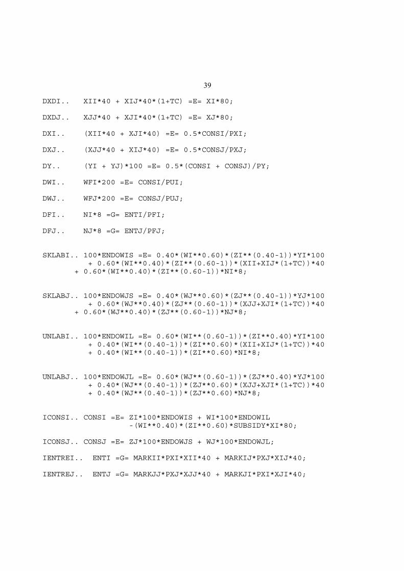
39

DXDI.. XII*40 + XIJ*40*(1+TC) =E= XI*80;

DXDJ.. XJJ*40 + XJI*40*(1+TC) =E= XJ*80;

DXI.. (XII*40 + XJI*40) =E= 0.5*CONSI/PXI;

DXJ.. (XJJ*40 + XIJ*40) =E= 0.5*CONSJ/PXJ;

DY.. (YI + YJ)*100 =E= 0.5*(CONSI + CONSJ)/PY;

DWI.. WFI*200 =E= CONSI/PUI;

DWJ.. WFJ*200 =E= CONSJ/PUJ;

DFI.. NI*8 =G= ENTI/PFI;

DFJ.. NJ*8 =G= ENTJ/PFJ;

SKLABI.. 100*ENDOWIS =E= 0.40*(WI**0.60)*(ZI**(0.40-1))*YI*100 + 0.60*(WI**0.40)*(ZI**(0.60-1))*(XII+XIJ*(1+TC))*40

+ 0.60*(WI**0.40)*(ZI**(0.60-1))*NI*8;

SKLABJ.. 100*ENDOWJS =E= 0.40*(WJ**0.60)*(ZJ**(0.40-1))*YJ*100 + 0.60*(WJ**0.40)*(ZJ**(0.60-1))*(XJJ+XJI*(1+TC))*40

+ 0.60*(WJ**0.40)*(ZJ**(0.60-1))*NJ*8;

UNLABI.. 100*ENDOWIL =E= 0.60*(WI**(0.60-1))*(ZI**0.40)*YI*100 + 0.40*(WI**(0.40-1))*(ZI**0.60)*(XII+XIJ*(1+TC))*40 + 0.40*(WI**(0.40-1))*(ZI**0.60)*NI*8;

UNLABJ.. 100*ENDOWJL =E= 0.60*(WJ**(0.60-1))*(ZJ**0.40)*YJ*100 + 0.40*(WJ**(0.40-1))*(ZJ**0.60)*(XJJ+XJI*(1+TC))*40 + 0.40*(WJ**(0.40-1))*(ZJ**0.60)*NJ*8;

ICONSI.. CONSI =E= ZI*100*ENDOWIS + WI*100*ENDOWIL -(WI**0.40)*(ZI**0.60)*SUBSIDY*XI*80;

ICONSJ.. CONSJ =E= ZJ*100*ENDOWJS + WJ*100*ENDOWJL;

IENTREI.. ENTI =G= MARKII*PXI*XII*40 + MARKIJ*PXJ*XIJ*40;

IENTREJ.. ENTJ =G= MARKJJ*PXJ*XJJ*40 + MARKJI*PXI*XJI*40;

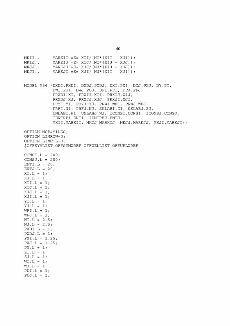
40

MKII.. MARKII =E= XII/(NI*(XII + XJI));MKIJ.. MARKIJ =E= XIJ/(NI*(XIJ + XJJ));MKJJ.. MARKJJ =E= XJJ/(NJ*(XIJ + XJJ));MKJI.. MARKJI =E= XJI/(NJ*(XII + XJI));

MODEL M54 /DXDI.PXDI, DXDJ.PXDJ, DXI.PXI, DXJ.PXJ, DY.PY, DWI.PUI, DWJ.PUJ, DFI.PFI, DFJ.PFJ, PRXDI.XI, PRXII.XII, PRXIJ.XIJ, PRXDJ.XJ, PRXJJ.XJJ, PRXJI.XJI, PRYI.YI, PRYJ.YJ, PRWI.WFI, PRWJ.WFJ, PRFI.NI, PRFJ.NJ, SKLABI.ZI, SKLABJ.ZJ, UNLABI.WI, UNLABJ.WJ, ICONSI.CONSI, ICONSJ.CONSJ, IENTREI.ENTI, IENTREJ.ENTJ, MKII.MARKII, MKIJ.MARKIJ, MKJJ.MARKJJ, MKJI.MARKJI/;


CONSI.L = 200;CONSJ.L = 200;ENTI.L = 20;ENTJ.L = 20;XI.L = 1;XJ.L = 1;XII.L = 1;XIJ.L = 1;XJJ.L = 1;XJI.L = 1;YI.L = 1;YJ.L = 1;WFI.L = 1;WFJ.L = 1;NI.L = 2.5;NJ.L = 2.5;PXDI.L = 1;PXDJ.L = 1;PXI.L = 1.25;PXJ.L = 1.25;PY.L = 1;ZI.L = 1;ZJ.L = 1;WI.L = 1;WJ.L = 1;PUI.L = 1;PUJ.L = 1;

41

PFI.L = 1;PFJ.L = 1;MARKII.L = 0.20;MARKIJ.L = 0.20;MARKJJ.L = 0.20;MARKJI.L = 0.20;

PY.FX = 1;


* counterfactual: trade costs of 15%

TC = 0.15;


* counterfactual: home production subsidy of 10%, trade costs 0

TC = 0.;SUBSIDY = .10;


* counterfactual: country's identical except for size,* positive trade costs (home market advantage)

SUBSIDY = 0;TC = 0.15;

ENDOWIL = 1.5;ENDOWJL = 0.5;ENDOWIS = 1.5;ENDOWJS = 0.5;


REALWI = WI.L/PUI.L;REALWJ = WJ.L/PUJ.L;REALZI = ZI.L/PUI.L;REALZJ = ZJ.L/PUJ.L;

DISPLAY REALWI, REALWJ, REALZI, REALZJ;

42

Model M54-MPS

As models get bigger, the advantages of MPS/GE become more and more obvious. It is

not just the amount of coding saved by using MPS/GE, but the avoidance of errors due to the fact

that MPS/GE automatically generates factor demands, income balance, and market clearing

conditions. It took me about 40 minutes to code the MPS/GE version of this model, and about

three or four hours to get the MCP version correct. Even then, I only knew that there were some

errors in the MCP version because results from a couple of the counterfactuals did not match

those from the MPS/GE version. I do think that it is very important for new modelers to code

MCP versions of simple problems, so that the modeler understands exactly what MPS/GE is

doing and exactly what square system is being generated in the background.

There is virtually nothing to add at this point. One thing that I might alert modelers to is

possible divide by zero errors that I have had to deal with in my models of multinationals. When

there are several types of firms, not all of which are active in equilibrium, there can be a divide-

by-zero problem in the markup equations with NI zero if there are no type-NI firms in

equilibrium. The simplest solution is just to set a lower bound on such a variable by using an

expression like

NI.LO = 0.0001;

before the solve statement. This in not perfectly satisfactory since if that firm type is not active,

some resources will still be consumed in fixed costs, but the approximation error is small. A

more sophisticated solution to this difficulty is found in appendix 5 of my book on multinational

firms (“Multinational Firms and the Theory of International Trade”, MIT press, 2002).

A related problem is if there is an entrepreneur who is the sole demander of a particular

(fixed cost) good and that firm type is not active, then there is no demand for that good. Then the

price of that good is zero, which in turn causes the solution algorithm problems insofar as that

prices may appear in the denominator of some expression in the solution routine. This problem

only occurs in the initialization of the model and is easily solved. In the case of this model, this

problem is easily solved by including the following statements before the solve statements to

ensure that the initial values of incomes are not zero.

FCI.L = MAX(FCI.L, 0.0001);FCJ.L = MAX(FCJ.L, 0.0001);


Note again the difference between the suffixes “.L” which stands for “level”, and sets the current

value of a variable but allows the variable full freedom to change, and “.LO” which stands for

“fix the lower bound of the variable at...”.

43

$TITLE: M54-MPS.GMS. Two country oligopoly model with free entry* uses MPS/GE

$ONTEXT


PYI 100 -100PYJ 100 -100PXI 100 -50 -50PXJ 100 -50 -50FCI 20 -20FCJ 20 -20 ZI -40 -48 -12 100ZJ -40 -48 -12 100WI -60 -32 -8 100WJ -60 -32 -8 100PUI 200 -200PUJ 200 -200MKI -10 -10 10 10MKJ -10 -10 10 10

$OFFTEXT

PARAMETERS ENDOWIL ENDOWJL ENDOWIS ENDOWJS REALWI REALWJ REALZI REALZJ TC SUBSIDY;

TC = .0;SUBSIDY = 0;ENDOWIL = 1;ENDOWJL = 1;ENDOWIS = 1;ENDOWJS = 1;

$ONTEXT$MODEL:M54

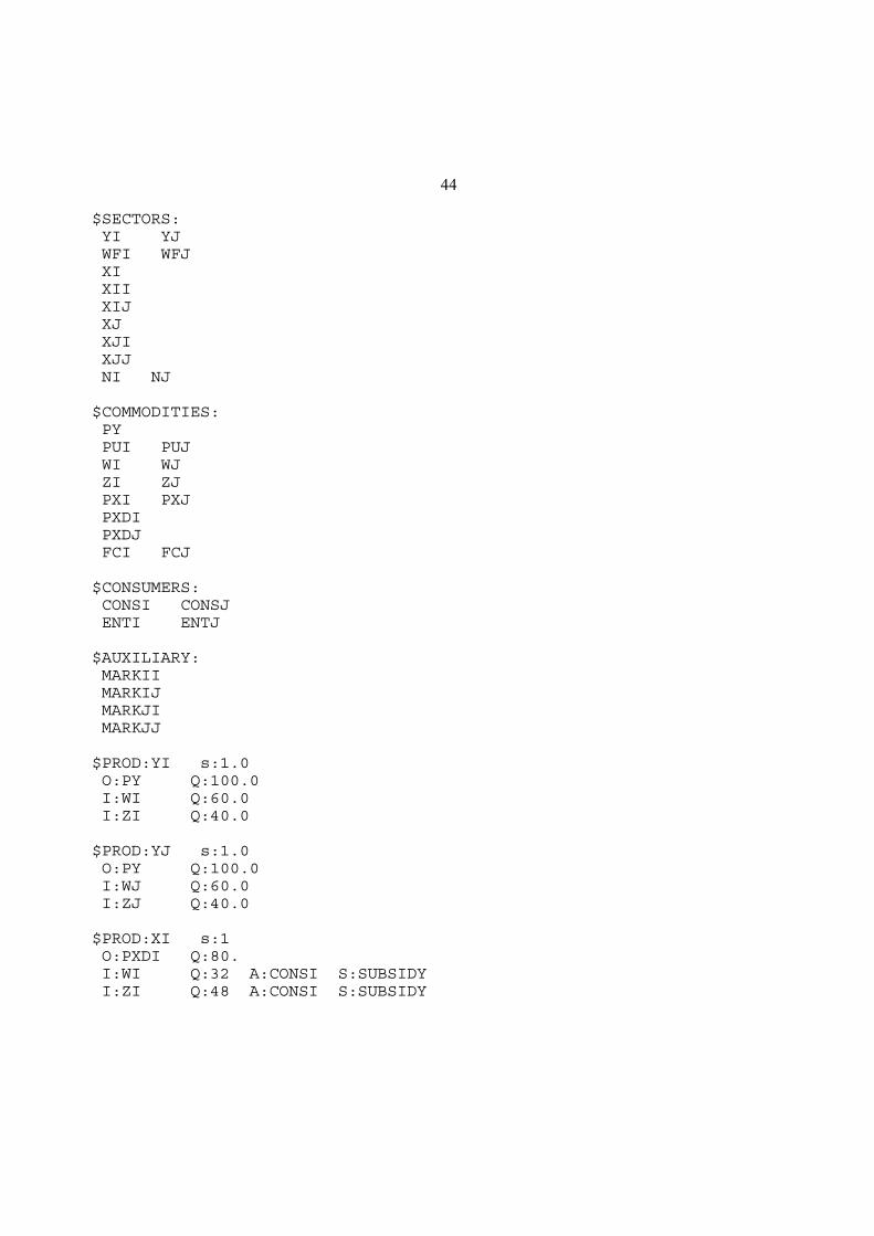
44

$SECTORS: YI YJ WFI WFJ XI XII XIJ XJ XJI XJJ NI NJ

$COMMODITIES: PY PUI PUJ WI WJ ZI ZJ PXI PXJ PXDI PXDJ FCI FCJ

$CONSUMERS: CONSI CONSJ ENTI ENTJ

$AUXILIARY: MARKII MARKIJ MARKJI MARKJJ

$PROD:YI s:1.0 O:PY Q:100.0 I:WI Q:60.0 I:ZI Q:40.0

$PROD:YJ s:1.0 O:PY Q:100.0 I:WJ Q:60.0 I:ZJ Q:40.0

$PROD:XI s:1 O:PXDI Q:80. I:WI Q:32 A:CONSI S:SUBSIDY I:ZI Q:48 A:CONSI S:SUBSIDY

45

$PROD:XII O:PXI Q:40. A:ENTI N:MARKII I:PXDI Q:40.

$PROD:XIJ s:0.0 O:PXJ Q:40. A:ENTI N:MARKIJ I:PXDI Q:(40.*(1+TC))

$PROD:XJ s:1 O:PXDJ Q:80. I:WJ Q:32. I:ZJ Q:48.

$PROD:XJI O:PXI Q:40. A:ENTJ N:MARKJI I:PXDJ Q:(40.*(1+TC))

$PROD:XJJ s:0.0 O:PXJ Q:40. A:ENTJ N:MARKJJ I:PXDJ Q:40.

$PROD:NI s:1 O:FCI Q:(20/2.5) I:WI Q:(8/2.5) I:ZI Q:(12/2.5)

$PROD:NJ s:1 O:FCJ Q:(20/2.5) I:WJ Q:(8/2.5) I:ZJ Q:(12/2.5)

$PROD:WFI s:1.0 O:PUI Q:200. I:PXI Q:80. P:1.25 I:PY Q:100.

$PROD:WFJ s:1.0 O:PUJ Q:200. I:PXJ Q:80. P:1.25 I:PY Q:100.

$DEMAND:CONSI D:PUI Q:200 E:WI Q:(100.*ENDOWIL) E:ZI Q:(100.*ENDOWIS)

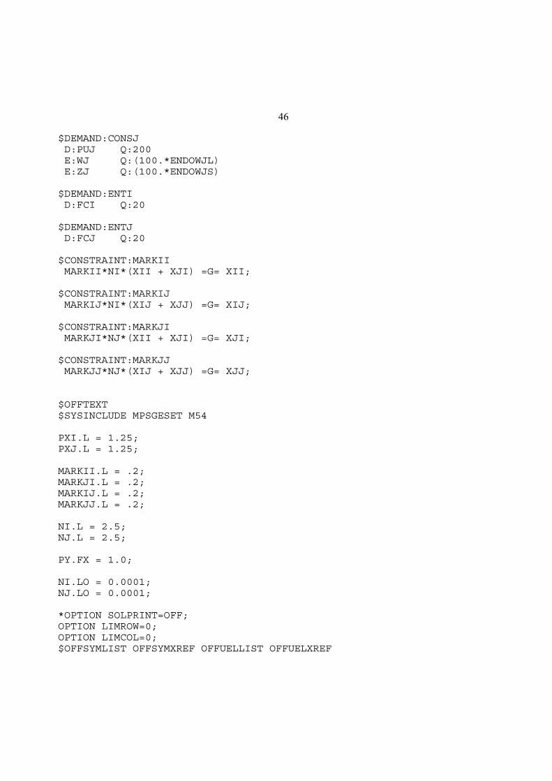
46

$DEMAND:CONSJ D:PUJ Q:200 E:WJ Q:(100.*ENDOWJL) E:ZJ Q:(100.*ENDOWJS)

$DEMAND:ENTI D:FCI Q:20

$DEMAND:ENTJ D:FCJ Q:20

$CONSTRAINT:MARKII MARKII*NI*(XII + XJI) =G= XII;

$CONSTRAINT:MARKIJ MARKIJ*NI*(XIJ + XJJ) =G= XIJ;

$CONSTRAINT:MARKJI MARKJI*NJ*(XII + XJI) =G= XJI;

$CONSTRAINT:MARKJJ MARKJJ*NJ*(XIJ + XJJ) =G= XJJ;

$OFFTEXT$SYSINCLUDE MPSGESET M54

PXI.L = 1.25;PXJ.L = 1.25;

MARKII.L = .2;MARKJI.L = .2;MARKIJ.L = .2;MARKJJ.L = .2;

NI.L = 2.5;NJ.L = 2.5;

PY.FX = 1.0;

NI.LO = 0.0001;NJ.LO = 0.0001;

*OPTION SOLPRINT=OFF;OPTION LIMROW=0;OPTION LIMCOL=0;$OFFSYMLIST OFFSYMXREF OFFUELLIST OFFUELXREF

47


* counterfactual: trade costs of 15%

TC = 0.15;


* counterfactual: home production subsidy of 10%, trade costs 0

TC = 0.;SUBSIDY = .10;


* counterfactual: country's identical except for size,* positive trade costs (home market advantage)

SUBSIDY = 0;TC = 0.15;

ENDOWIL = 1.5;ENDOWJL = 0.5;ENDOWIS = 1.5;ENDOWJS = 0.5;




1

Chapter 6

External Economies and Monopolistic Competition

Now we continue our study of increasing returns to scale, turning to models based on

external economies of scale and monopolistic-competition models. I have grouped these two

together in one chapter since there are close technical similarities between them. A formal

demonstration of this equivalence is found in Markusen (CJE vol. 23, 1990, 495-508.).

These models require a few tricks to code in MPS/GE, because MPS/GE requires all

activities to have constant returns to scale. Because of this, I want to present MCP versions of

the models first, in order to show clearly what equations and inequalities are being solved. Then

I present the MPS/GE versions and show the tricks. In very simple models such as the ones

presented here, it is generally easiest to stick with the MCP solver and not use the higher-level

language. But it more complicated higher-dimension models, it is best to learn the tricks and use

MPS/GE.

Models are as follows:

M61-MCP.GMS Closed economy external economies of scale, MCP version

M61-MPS.GMS Closed economy external economies of scale, MPS/GE version

M62-MCP.GMS Closed economy large-group monopolistic competition, MCP version

M62-MPS.GMS Closed economy large-group monopolistic competition, MPS/GE verion

M63-MPC.GMS Two-country model with large-group monopolistic competition, MCP

version

M63-MPC.GMS Two-country model with large-group monopolistic competition, MPS/GE

version

2

Model M61-MCP

The theoretical foundations of this model go back to the 1960s with work by Kemp and

Melvin. The idea is that the production function for an individual firm is given by

(1) Xi

(X )F (Vi) 0 < < 1

where Xi is firm i’s output, X is the sum of all firms' output (industry output), F is a function with

constant returns to scale, and Vi is the firm's vector of inputs.

The parameter β reflects industry level scale economies, with β = 0 being the special case

of constant returns to scale.

By virtue of the fact that F( ) has constant returns to scale and is identical for all firms, total

industry output can then be written as:

(2) X ( X )F (V ) or X F (V )1/(1 )

so X industry output is homogeneous of degree 1/(1 - β) > 1 in primary factor inputs.

To make the point in the simplest fashion, assume that there is just a single factor L with

a price w. p denotes the price of X. Each individual firm views total industry output as constant,

and thus each firm views itself as producing with constant returns to scale. The firm’s

optimization condition equates the value of the (private) marginal product of labor to the wage

rate.

(3) pXdX

i

dLi

w p X wdL

i

dXi

X c (w )

where c(w) is the cost of one “factor bundle”, the cost of labor needed to produce F(L) = 1. That

is, c(w) is the unit cost function associated with the constant-returns function F(L). This then

becomes the pricing equation or zero profit condition for the X sector in the MCP.

The other thing that we need for the market-clearing condition for labor in the MCP is the

total demand for labor in the X sector. This is given by the amount of labor needed for F(L) = 1

times F(L). The unit requirement is given as usual by Shephard’s lemma, the derivative of the

unit cost function. So using (1), the demand for labor in the X sector is given by

(4) c (w )F (L ) c (w )X 1

The demand for labor is concave in output, the dual of increasing returns in production.

3

Here is the data matrix for the model, the same one that we have used before:

Production Sectors Consumers Markets | X Y W | CONS ------------------------------------------------------ PX | 100 -100 | PY | 100 -100 | PU | 200 | -200 PW | -40 -60 | 100 PZ | -60 -40 | 100 ------------------------------------------------------

We will assume that the production functions are Cobb-Douglas. Units will be chosen

such that X = 1 initially, which then greatly simplifies the calibration of the data to the model.

The letter “B” is used in place of beta. For some historical reasons now forgotten, PU now

denotes the price of utility (welfare), PW is the price of unskilled labor, and the other factor is

now called skilled labor, with a price of PZ.

The following block of code is inserted in order to suppress a lot of output in the listing

file and you can certainly ignore it for now. But it is valuable in a program with many solve

statements.

OPTION LIMROW=0;OPTION LIMCOL=0;$OFFSYMLIST OFFSYMXREF OFFUELLIST OFFUELXREF

Here is the model.

4

$TITLE: Model M61-MCP: External Economies of Scale, uses MCP

$ONTEXT

The model is based on the benchmark social accounts for model M1-1:


$OFFTEXT

PARAMETERSBENDOWSENDOWLMODELSTAT;

ENDOWS = 100;ENDOWL = 100;B = 0.2;

POSITIVE VARIABLESXYWPXPYPUPZPWCONS;

EQUATIONSDX Demand for XDY Demand for YDW Demand for WPRICEX MR = MC in XPRICEY Zero profit condition for Y (PY = MC)PRICEW Zero profit condition for WSKLAB Supply-demand balance for skilled labor

5

UNLAB Supply-demand balance for unskilled laborINCOME National income;

PRICEX.. (PW**0.40)*(PZ**0.60)/(X**B) =G= PX;

PRICEY.. (PW**0.60)*(PZ**0.40) =G= PY;

PRICEW.. (PX**0.50)*(PY**0.50) =G= PU;

DX.. X*100 =E= CONS/(2*PX);

DY.. Y*100 =E= CONS/(2*PY);

DW.. 200*W =E= CONS/PU;

SKLAB.. ENDOWS =E= 0.40*(PW**0.60)*(PZ**(0.40-1))*Y*100 + 0.60*(PW**0.40)*(PZ**(0.60-1))*(X**(1-B))*100;

UNLAB.. ENDOWL =E= 0.60*(PW**(0.60-1))*(PZ**0.40)*Y*100 + 0.40*(PW**(0.40-1))*(PZ**0.60)*(X**(1-B))*100;

INCOME.. CONS =E= PZ*ENDOWS + PW*ENDOWL;

MODEL M61 /DX.PX, DY.PY, DW.PU, PRICEX.X, PRICEY.Y, PRICEW.W, SKLAB.PZ, UNLAB.PW, INCOME.CONS/;


CONS.L = 200;X.L = 1;Y.L = 1;W.L = 1;PX.L = 1;PY.L = 1;PZ.L = 1;PW.L = 1;PU.L = 1;

PY.FX = 1;

6

SOLVE M61 USING MCP;MODELSTAT = M61.MODELSTAT - 1.;

DISPLAY MODELSTAT;

* Counterfactual: expand the size of the economy

ENDOWS = 200;ENDOWL = 200;


* Counterfactual: contract the size of the economy

ENDOWS = 80;ENDOWL = 80.


The counterfactual-experiments involve changing the size of the economy. The first

experiment doubles the size of the economy. This increases the welfare index from 1.000 to

2.181, more than double its initial value representing the scale economies in production.

7

Model M61-MPS

The difficulty for translating this model into MPS/GE is that this higher-level language

requires constant returns to scale in all activities so that it can generate cost functions and factor

demands in a standardized way. There are a couple of tricks that get around this. They may

seem awkward and not worth the bother in such a small model, but in big models with many

sectors, factors, or countries it is well worth learning the tricks.

How do we model this given that MPS/GE requires constant returns to scale? We will

use a trick, in which the X industry produces X0 = F(V0) so that the X sector output is now the

constant returns function F using factor bundles. Then we will "give" the consumer an additional

amount equal to the “true” industry output minus the output from factor bundles.

(5) X1

X1/ (1 )

0 X0

Then the consumer actually receives

(6) .X X1

X0

F (V0)1/ (1 )

The value of X1 is determined by the auxiliary variable XQADJ (X quantity adjustment = X1) in

the program that follows. It is important to note that the value of X listed in the output file of

the program is what is called X0, not the true output of X.

But now we have an imbalance in that the value of X received by the consumer is more

than the value of X produced by the firms. So we will subsidize X production so that the value

of payments received by the firm for X0 is equal to the value of X= X1 + X0 consumed by the

consumer. Let q denote the consumer price and p the producer price of X. Let q be the tax base,

so q(1-s) = p. For payments to balance, we need

(7) q (X1/ (1 )

0 ) pX0

or (1 s ) X/ (1 )

0

(8) s X/ (1 )

0 1 or s XQADJ /X0

s is determined in the model to follow by the auxiliary variable XPADJ.

The model is calibrated so that all activity levels are one initially, implying that the initial

values of XQADJ and XPADJ are zero initially. β = .2, β/(1-β) = .25

Counterfactual experiments change the size of the economy. Notice the consequences of

the scale economies.

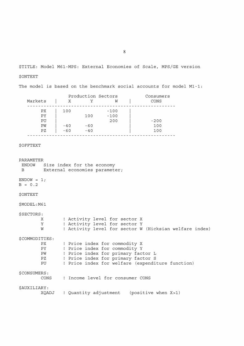
8

$TITLE: Model M61-MPS: External Economies of Scale, MPS/GE version

$ONTEXT

The model is based on the benchmark social accounts for model M1-1:


$OFFTEXT

PARAMETER ENDOW Size index for the economy B External economies parameter;

ENDOW = 1;B = 0.2

$ONTEXT

$MODEL:M61


$COMMODITIES: PX ! Price index for commodity X PY ! Price index for commodity Y PW ! Price index for primary factor L PZ ! Price index for primary factor S PU ! Price index for welfare (expenditure function)


$AUXILIARY: XQADJ ! Quantity adjustment (positive when X>1)

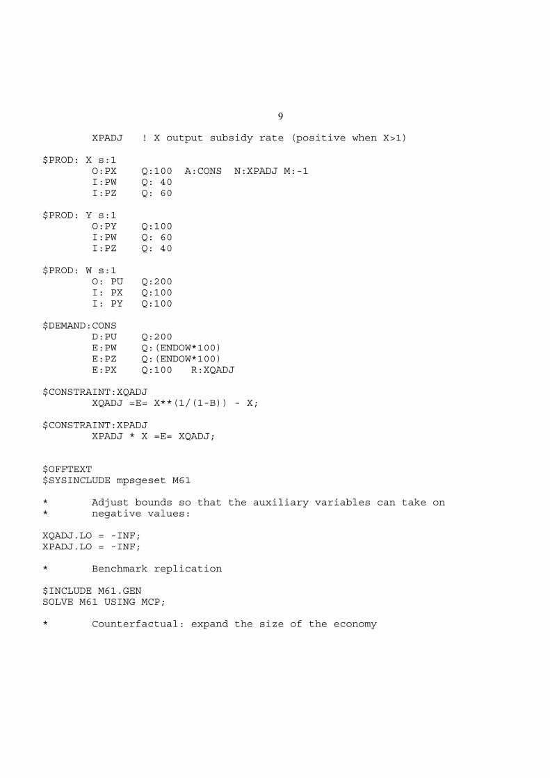
9

XPADJ ! X output subsidy rate (positive when X>1)

$PROD: X s:1 O:PX Q:100 A:CONS N:XPADJ M:-1 I:PW Q: 40 I:PZ Q: 60

$PROD: Y s:1 O:PY Q:100 I:PW Q: 60 I:PZ Q: 40

$PROD: W s:1 O: PU Q:200 I: PX Q:100 I: PY Q:100

$DEMAND:CONS D:PU Q:200 E:PW Q:(ENDOW*100) E:PZ Q:(ENDOW*100) E:PX Q:100 R:XQADJ

$CONSTRAINT:XQADJ XQADJ =E= X**(1/(1-B)) - X;

$CONSTRAINT:XPADJ XPADJ * X =E= XQADJ;


* Adjust bounds so that the auxiliary variables can take on * negative values:

XQADJ.LO = -INF;XPADJ.LO = -INF;




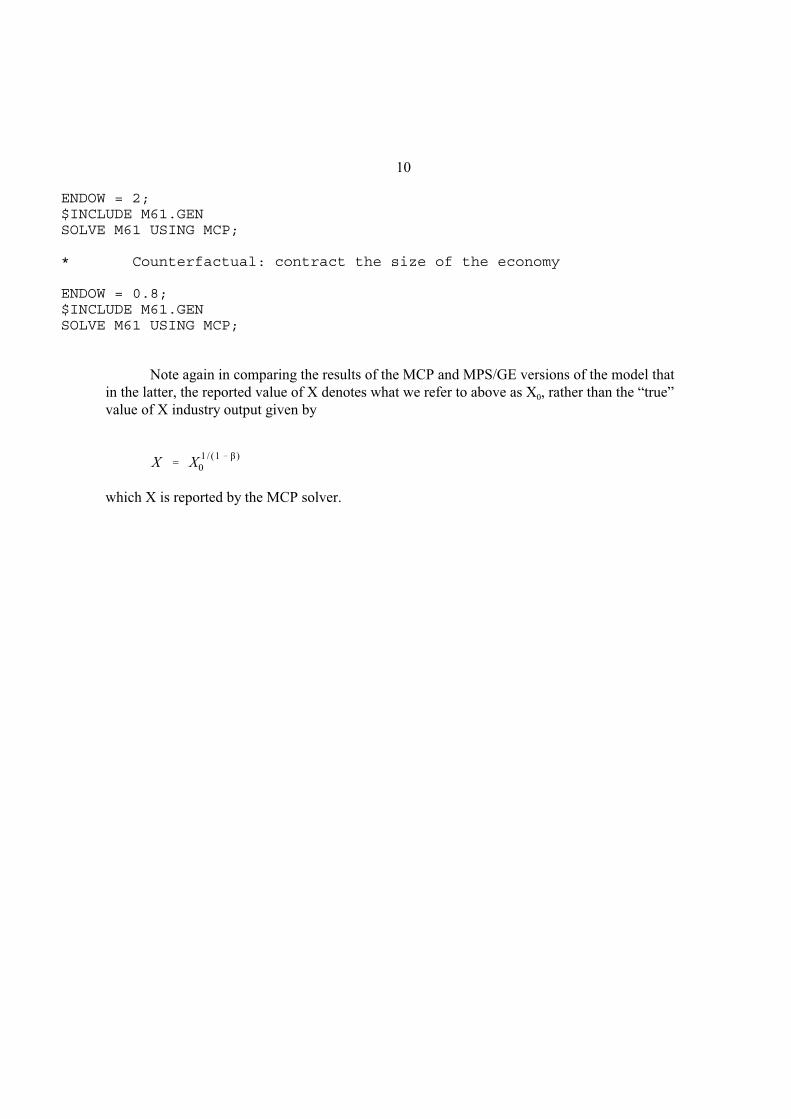
10

ENDOW = 2;$INCLUDE M61.GENSOLVE M61 USING MCP;

* Counterfactual: contract the size of the economy

ENDOW = 0.8;$INCLUDE M61.GENSOLVE M61 USING MCP;

Note again in comparing the results of the MCP and MPS/GE versions of the model that

in the latter, the reported value of X denotes what we refer to above as X0, rather than the “true”

value of X industry output given by

X X1/ (1 )

0

which X is reported by the MCP solver.

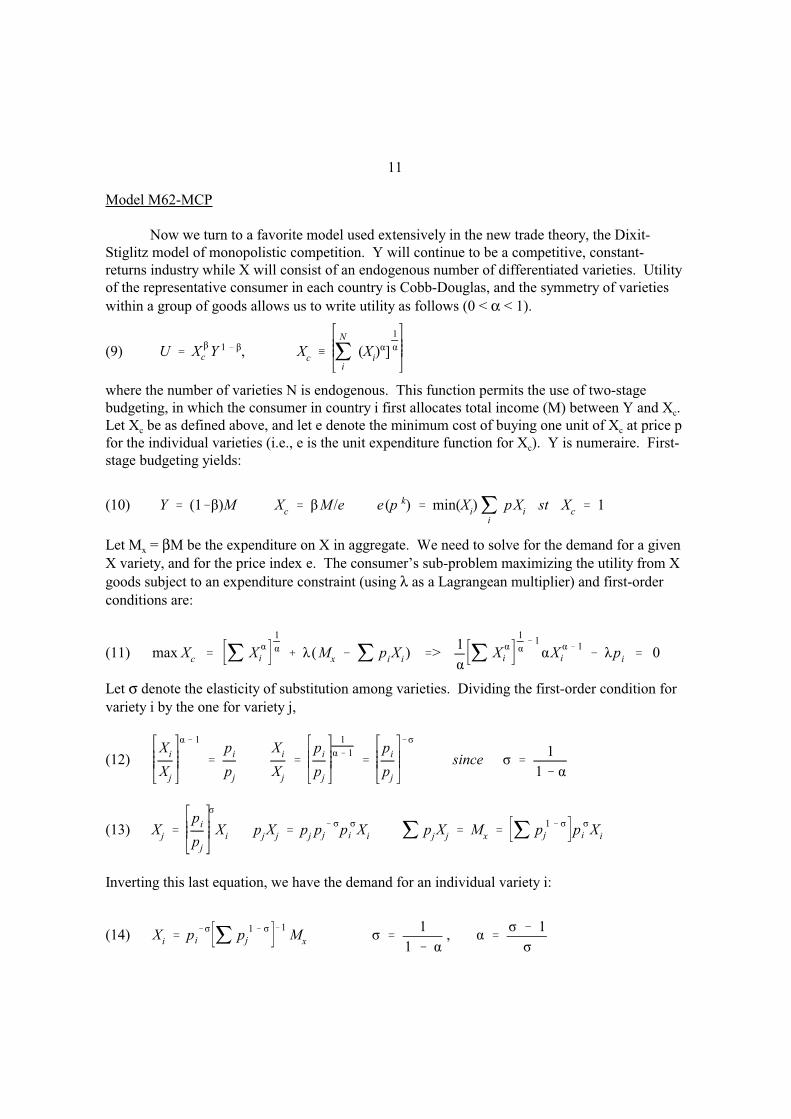
11

Model M62-MCP

Now we turn to a favorite model used extensively in the new trade theory, the Dixit-

Stiglitz model of monopolistic competition. Y will continue to be a competitive, constant-

returns industry while X will consist of an endogenous number of differentiated varieties. Utility

of the representative consumer in each country is Cobb-Douglas, and the symmetry of varieties

within a group of goods allows us to write utility as follows (0 < α < 1).

(9) U Xc Y 1 , Xc

N

i

(Xi) ]

1

where the number of varieties N is endogenous. This function permits the use of two-stage

budgeting, in which the consumer in country i first allocates total income (M) between Y and Xc.

Let Xc be as defined above, and let e denote the minimum cost of buying one unit of Xc at price p

for the individual varieties (i.e., e is the unit expenditure function for Xc). Y is numeraire. First-

stage budgeting yields:

(10) Y (1 )M Xc

M /e e (p k) min(Xi)

i

pXi

st Xc

1

Let Mx = βM be the expenditure on X in aggregate. We need to solve for the demand for a given

X variety, and for the price index e. The consumer’s sub-problem maximizing the utility from X

goods subject to an expenditure constraint (using λ as a Lagrangean multiplier) and first-order

conditions are:

(11) max Xc

Xi

1

(Mx

piX

i) >

1Xi

11

X1

i pi

0

Let σ denote the elasticity of substitution among varieties. Dividing the first-order condition for

variety i by the one for variety j,

(12)X

i

Xj

1p

i

pj

Xi

Xj

pi

pj

1

1 pi

pj

since1

1

(13) Xj

pi

pj

Xi

pjX

jp

jpj pi X

ip

jX

jM

xp

1

j pi Xi

Inverting this last equation, we have the demand for an individual variety i:

(14) Xi

pi p1

j

1M

x

1

1,

1

12

Now we can use Xi to construct Xc and then solve for e, noting the relationship between α and σ.

(15) Xi X

1

i p1

i p1

j

1

Mx

(16) Xi p1

i p1

j

1

Mx p1

j

1

Mx

(17) Xc

Xi

1

Xi1 p

1

j

1

1 Mx

(18) e p1

j

1

1

Having derived e, we can then use equation (13) in (9) to get the demand for an individual

variety.

(19) Xi

pi e 1 Mx

since e 1 p1

j

1

The usual assumption in “large-group” monopolistic competition is that there are many

firms such that individual firms view e and M as constants. Thus the elasticity of demand for an

individual variety is just σ. Equilibrium in the X sector involves two equations in two

unknowns. The unknowns are X, output per variety and N, the numbers of varieties or firms.

The two equations are the firm’s optimization condition, marginal revenue equals marginal cost,

and the free-entry or zero profit condition, prices equals average cost. Let c(w,z) denote marginal

cost where w and z are the prices of skilled and unskilled labor respectively. Let F(w,z) denote

fixed costs per firm. The two equations are given by

(20) p (1 1/ ) c (w , z ) p c (w , z ) F (w , z ) /X

(21)1

(1 1/ )1

F (w , z )

c (w, z )X

which simplifies to

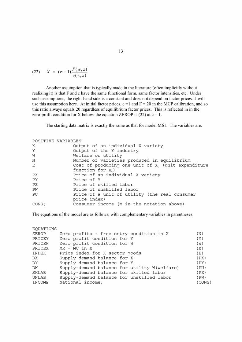
13

(22) X ( 1)F (w , z )

c (w, z )

Another assumption that is typically made in the literature (often implicitly without

realizing it) is that F and c have the same functional form, same factor intensities, etc. Under

such assumptions, the right-hand side is a constant and does not depend on factor prices. I will

use this assumption here. At initial factor prices, c =1 and F = 20 in the MCP calibration, and so

this ratio always equals 20 regardless of equilibrium factor prices. This is reflected in in the

zero-profit condition for X below: the equation ZEROP is (22) at c = 1.

The starting data matrix is exactly the same as that for model M61. The variables are:

POSITIVE VARIABLESX Output of an individual X varietyY Output of the Y industryW Welfare or utilityN Number of varieties produced in equilibriumE Cost of producing one unit of Xc (unit expenditure

function for Xc)PX Price of an individual X varietyPY Price of YPZ Price of skilled laborPW Price of unskilled laborPU Price of a unit of utility (the real consumer

price index)CONS; Consumer income (M in the notation above)

The equations of the model are as follows, with complementary variables in parentheses.

EQUATIONSZEROP Zero profits - free entry condition in X (N)PRICEY Zero profit condition for Y (Y)PRICEW Zero profit condition for W (W)PRICEX MR = MC in X (X)INDEX Price index for X sector goods (E)DX Supply-demand balance for X (PX)DY Supply-demand balance for Y (PY)DW Supply-demand balance for utility W(welfare) (PU)SKLAB Supply-demand balance for skilled labor (PZ)UNLAB Supply-demand balance for unskilled labor (PW)INCOME National income; (CONS)

14

Here again we see the logic of associating zero profit or pricing equations with quantity

variables, and market clearing conditions with price.

One thing that is slightly misleading is to call the ZEROP equation “zero profits in X”. In

the code to follow this is the equation for equilibrium output per firm in the X industry which is

derived from using both the zero-profit condition and the pricing equation. This is not really

necessary and we could just use the zero-profit condition here.

The code of the model follows:

15

$TITLE: Model M62-MCP: Large-Group Monopolistic Competition: uses MCP

$ONTEXT

Production Sectors Consumers Markets | XC X N Y W | CONS ENTR

---------------------------------------------------------------------- PX | 100 -100 | CX ! 100 -100 | PY | 100 -100 | PF | 20 | -20 PU | 200 | -200 PW | -32 -8 -60 | 100 PZ | -48 -12 -40 | 100 MK | -20 | 20

$OFFTEXT

PARAMETERSEPFCENDOWSENDOWLWELFAREMODELSTAT;

EP = 5;FC = 20;ENDOWS = 100;ENDOWL = 100;

POSITIVE VARIABLESXYWNEPXPYPZPWPUCONS;

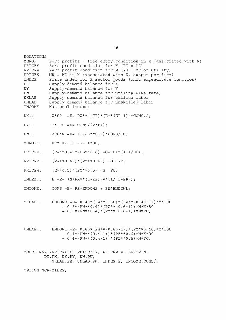
16

EQUATIONSZEROP Zero profits - free entry condition in X (associated with N)PRICEY Zero profit condition for Y (PY = MC)PRICEW Zero profit condition for W (PU = MC of utility)PRICEX MR = MC in X (associated with X, output per firm)INDEX Price index for X sector goods (unit expenditure function)DX Supply-demand balance for XDY Supply-demand balance for YDW Supply-demand balance for utility W(welfare)SKLAB Supply-demand balance for skilled laborUNLAB Supply-demand balance for unskilled laborINCOME National income;

DX.. X*80 =E= PX**(-EP)*(E**(EP-1))*CONS/2;

DY.. Y*100 =E= CONS/(2*PY);

DW.. 200*W =E= (1.25**0.5)*CONS/PU;

ZEROP.. FC*(EP-1) =G= X*80;

PRICEX.. (PW**0.4)*(PZ**0.6) =G= PX*(1-1/EP);

PRICEY.. (PW**0.60)*(PZ**0.40) =G= PY;

PRICEW.. (E**0.5)*(PY**0.5) =G= PU;

INDEX.. E =E= (N*PX**(1-EP))**(1/(1-EP));

INCOME.. CONS =E= PZ*ENDOWS + PW*ENDOWL;

SKLAB.. ENDOWS =E= 0.40*(PW**0.60)*(PZ**(0.40-1))*Y*100 + 0.6*(PW**0.4)*(PZ**(0.6-1))*N*X*80 + 0.6*(PW**0.4)*(PZ**(0.6-1))*N*FC;

UNLAB.. ENDOWL =E= 0.60*(PW**(0.60-1))*(PZ**0.40)*Y*100 + 0.4*(PW**(0.4-1))*(PZ**0.6)*N*X*80 + 0.4*(PW**(0.4-1))*(PZ**0.6)*N*FC;

MODEL M62 /PRICEX.X, PRICEY.Y, PRICEW.W, ZEROP.N, DX.PX, DY.PY, DW.PU,

SKLAB.PZ, UNLAB.PW, INDEX.E, INCOME.CONS/;

OPTION MCP=MILES;

17

OPTION LIMROW=0;OPTION LIMCOL=0;$OFFSYMLIST OFFSYMXREF OFFUELLIST OFFUELXREF

E.L = 1.25;CONS.L = 200;X.L = 1;Y.L = 1;N.L = 1;W.L = 1;PX.L = 1.25;PY.L = 1;PZ.L = 1;PW.L = 1;PU.L = 1.25**0.5;

PY.FX = 1;


DISPLAY MODELSTAT;


ENDOWS = 200;ENDOWL = 200;


The counter-factual experiment doubles the size of the economy. Note that the results are

exactly the same as in the external-economies model M61 (although remember that here X is

output per firm whereas earlier it referred to total output). These models are in fact operationally

identical, as I showed in my 1990 CJE article referenced earlier. In both cases, the X sector’s

output is homogeneous of degree 1.25 in factor inputs, if by X sector’s output here we mean Xc.

The X sector expands only through the entry of new firms and Xc is given by

and in the external economies model by Xc

n 1/ X X F (V )

1

1

where X in the first equation is a constant. Thus α = 0.8 (s = 5) in this model is exactly

equivalent to the external economies model with β = 0.2.

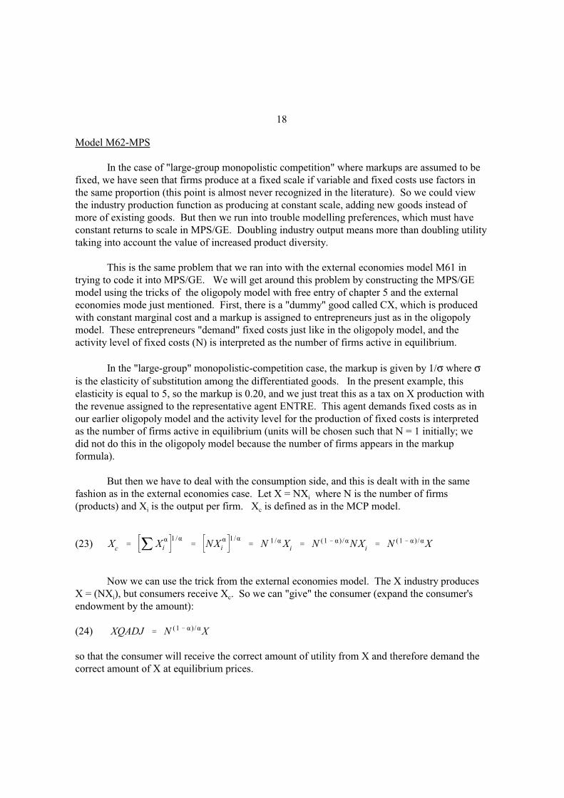
18

Model M62-MPS

In the case of "large-group monopolistic competition" where markups are assumed to be

fixed, we have seen that firms produce at a fixed scale if variable and fixed costs use factors in

the same proportion (this point is almost never recognized in the literature). So we could view

the industry production function as producing at constant scale, adding new goods instead of

more of existing goods. But then we run into trouble modelling preferences, which must have

constant returns to scale in MPS/GE. Doubling industry output means more than doubling utility

taking into account the value of increased product diversity.

This is the same problem that we ran into with the external economies model M61 in

trying to code it into MPS/GE. We will get around this problem by constructing the MPS/GE

model using the tricks of the oligopoly model with free entry of chapter 5 and the external

economies mode just mentioned. First, there is a "dummy" good called CX, which is produced

with constant marginal cost and a markup is assigned to entrepreneurs just as in the oligopoly

model. These entrepreneurs "demand" fixed costs just like in the oligopoly model, and the

activity level of fixed costs (N) is interpreted as the number of firms active in equilibrium.

In the "large-group" monopolistic-competition case, the markup is given by 1/σ where σis the elasticity of substitution among the differentiated goods. In the present example, this

elasticity is equal to 5, so the markup is 0.20, and we just treat this as a tax on X production with

the revenue assigned to the representative agent ENTRE. This agent demands fixed costs as in

our earlier oligopoly model and the activity level for the production of fixed costs is interpreted

as the number of firms active in equilibrium (units will be chosen such that N = 1 initially; we

did not do this in the oligopoly model because the number of firms appears in the markup

formula).

But then we have to deal with the consumption side, and this is dealt with in the same

fashion as in the external economies case. Let X = NXi where N is the number of firms

(products) and Xi is the output per firm. Xc is defined as in the MCP model.

(23) Xc

Xi

1/NXi

1/N 1/ X

iN (1 ) / NX

iN (1 ) / X

Now we can use the trick from the external economies model. The X industry produces

X = (NXi), but consumers receive Xc. So we can "give" the consumer (expand the consumer's

endowment by the amount):

(24) XQADJ N (1 ) / X

so that the consumer will receive the correct amount of utility from X and therefore demand the

correct amount of X at equilibrium prices.

19

Finally, we have the same problem as in the external economies case, we must have the

value of X received by the consumer equal to the payments received by the producer. Therefore,

the consumer has to subsidize the producer of X so that producer revenue equals the payments

for X made by the producer.

As in the external economies model, let q be the consumer price, and p be the producer

price. We must have

q N (1 ) / X pX q (1 s )X

So we must have

s N (1 ) / 1

This is given by the endogenous tax rate XPADJ (in the N: field) in the model to follow. Since α

= 0.8, σ = 5, the value of s is s = .25 = (1- α)/α.

To avoid having an ad valorem subsidy multiplied on top of an ad valorem tax (the

markup in activity XI), we just specify another activity, simply called X. X produces one unit of

"final good" PX for each unit of "intermediate good "CX". PX is the good that enters welfare

and demand.

The counter-factual experiment in the program that follows doubles the size of the

economy. The activity levels for X, XI, and N all double, but welfare more than doubles,

reflecting the increased value of product diversity (W = 2.18). For comparison to the MCP

version of this model, I also calculate the price index, e, for Xc which is generated after the model

solves. This is declared as the parameter INDEX.

20

$TITLE: Model M62-MPS: Large-Group Monopolistic Competition, uses MPS/GE

$ONTEXT

Production Sectors Consumers Markets | XI X N Y W | CONS ENTR

---------------------------------------------------------------------- PX | 100 -100 | CX ! 100 -100 | PY | 100 -100 | PF | 20 | -20 PU | 200 | -200 PW | -32 -8 -60 | 100 PZ | -48 -12 -40 | 100 MK | -20 | 20

$OFFTEXT

PARAMETERS ENDOW Size index for the economy INDEX Price index for the X goods EP Elasticity of substitution among X varieties;

ENDOW = 1;EP = 5;

$ONTEXT

$MODEL:M62

$SECTORS: X ! Activity level for sector X Y ! Activity level for sector Y W ! Activity level for sector W (Hicksian welfare index) N ! Activity level for sector X fixed costs, no. of firms XI ! Activity level -- marginal cost of X

$COMMODITIES: PX ! Price index for commodity X (gross of markup) CX ! Marginal cost index for commodity X (net markup) PY ! Price index for commodity Y PW ! Price index for unskilled labor PZ ! Price index for skilled labor PF ! Unit price of inputs to fixed cost PU ! Price index for welfare (expenditure function)

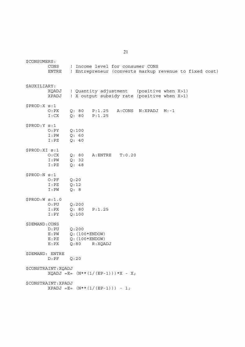
21

$CONSUMERS: CONS ! Income level for consumer CONS ENTRE ! Entrepreneur (converts markup revenue to fixed cost)

$AUXILIARY: XQADJ ! Quantity adjustment (positive when X>1) XPADJ ! X output subsidy rate (positive when X>1)

$PROD:X s:1 O:PX Q: 80 P:1.25 A:CONS N:XPADJ M:-1 I:CX Q: 80 P:1.25


$PROD:XI s:1 O:CX Q: 80 A:ENTRE T:0.20 I:PW Q: 32 I:PZ Q: 48

$PROD:N s:1 O:PF Q:20 I:PZ Q:12 I:PW Q: 8

$PROD:W s:1.0 O:PU Q:200 I:PX Q: 80 P:1.25 I:PY Q:100

$DEMAND:CONS D:PU Q:200 E:PW Q:(100*ENDOW) E:PZ Q:(100*ENDOW) E:PX Q:80 R:XQADJ

$DEMAND: ENTRE D:PF Q:20

$CONSTRAINT:XQADJ XQADJ =E= (N**(1/(EP-1)))*X - X;

$CONSTRAINT:XPADJ XPADJ =E= (N**(1/(EP-1))) - 1;

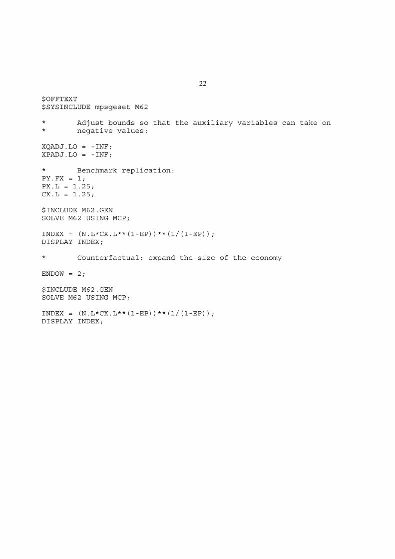
22


* Adjust bounds so that the auxiliary variables can take on * negative values:

XQADJ.LO = -INF;XPADJ.LO = -INF;

* Benchmark replication:PY.FX = 1;PX.L = 1.25; CX.L = 1.25;


INDEX = (N.L*CX.L**(1-EP))**(1/(1-EP));DISPLAY INDEX;


ENDOW = 2;


INDEX = (N.L*CX.L**(1-EP))**(1/(1-EP));DISPLAY INDEX;

23

Model M63-MCP

Now I present a two-country version of the monopolistic-competition model. This model

has been popular in trade theory and in the so-called new economic geography literature. The

countries will be labeled with subscripts i and j. X’s will carry double subscripts where the first

is the country of production and the second is the country of consumption. Thus Xij is X

produced in i and exported to j where it is consumed.

Trade costs are important in the literatures just referred to, so we will want to consider

these in our model. It has been popular to use “iceberg” trade costs where some of the good

“melts” in transit. The first thing to note is how iceberg trade costs are reflected in prices and

demand. For a domestic firm, Xij is the amount produced in country i and shipped to country j.

Let t (t > 1) be the ratio of the amount of X exported to the amount that arrives “unmelted”.

Alternatively 1/t is the proportion of a good that “survives” transit (the proportion “unmelted”).

If Xij is shipped, the amount received in country j is Xij/t.

Second, we make the usual assumption that there is no price discrimination and so the

home price of a good for local sales equals its export price. Thus we can use the notation pi and

pj for the price of all goods produced in country i and country j respectively. The revenues

received by the exporter are equal to the costs paid by the importer: piXij is the revenue received

by the exporter and Xij/t are the number of units arriving in the importing country, so the price

per unit in the importing country must be pit ( piXij = (pit)X ij/t ). Rather than introduce additional

notation, we will therefore use Xij/t and pit as the quantity and price in country j of a country i

variety exported to country j.

The price index for country i is then given by:

(15)ei

Nip

1

i Nj(p

jt )1

1

1

The various X varieties sold in country i are given by:

(16)Xii

pi e1

i Mix

Xji/ t (p

jt) e

1

i Mix

where the second equation can also be written as:

(17)Xji

pj t 1 e1

i Mix

There are few other complications beyond those discussed in the closed economy model

M62-MCP. The model is calibrated to trade free with the countries identical initially. Since X is

24

differentiated, it must therefore be the case that half of each firm’s output is sold in its home

country and half is exported. There are some numerical coefficients in the problem used to

adjust units so that most prices are one initially; this is not necessary but makes the output file

more comparable to the MPS/GE version that follows. This arises because I set the number of

firms in each country to 1 initially, so that the total number is 2. But if the price of an individual

variety is 1, then the price index in each country cannot be equal to 1. I thus use a units

adjustment in the equations for WELFAREI, WELFAREJ, PUI and PUJ in order that these all

take the value of 1 initially.

Several counterfactual experiments are considered at the end. First, we double the size of

the economies and see that there welfare more than doubles. In the second experiment, we return

the economy to its original size but set the trade cost at TC = 1.15. This reduces welfare by 3%

in each country as consumption of home versus imported goods becomes more unbalanced. The

third experiment has country i twice as large as country j, but no trade costs. Welfare is the same

for both countries (per capita) in free trade.

The fourth experiment has country i three times the size of j, but with trade costs TC =

1.15. Here we see some results found in the newer theory literature. There is a “home market

effect” whereby country i is better off and has more firms on a per capita basis than country j. At

the end of this experiment, we calculate real factor prices in each country by dividing the nominal

prices by the real consumer prices indices, the cost of buying one unit of utility. We see that in

spite of the countries having identical relative endowments, country i has a higher real price for

skilled labor and country j has a higher real price for unskilled labor. Thus this equilibrium is not

going to be stable under factor mobility, and skilled labor should flow toward country i

increasing further its specialization in X.

The final experiment retains the trade costs, gives both countries the same amount of

unskilled labor, but country i has 60% of the skilled labor and country j 40%. If you look at the

very end of the listing file, you see that country i has higher real prices for both factors, an

outcome noted by Markusen and Venables (JIE 2000).

25

$TITLE: Model M63: Two Country Large-Group Monopolistic Competition* uses MCP

$ontext

YI YJ XMI XMJ NMI NMJ WI WJ CONI CONJ EHTI ENTJ

PYI 100 -100PYJ 100 -100PXI 100 -50 -50PXJ 100 -50 -50FCI 20 -20FCJ 20 -20 ZI -40 -48 -12 100ZJ -40 -48 -12 100WI -60 -32 -8 100WJ -60 -32 -8 100UTILI 200 -200UTILJ 200 -200MKI -10 -10 10 10MKJ -10 -10 10 10

$offtext

PARAMETERSEPEYTCFCENDOWISENDOWILENDOWJSENDOWJLMODELSTAT;

EP = 5;EY = 3;TC = 1.;FC = 20;ENDOWIS = 100;ENDOWIL = 100;ENDOWJS = 100;ENDOWJL = 100;

POSITIVE VARIABLESWFI

26

WFJXIIXIJXJJXJIYIYJNINJPIPJPYPUIPUJEIEJZIWIZJWJMIMJ;

EQUATIONSWELFAREIWELFAREJDXIIDXJIDXJJDXIJDYZEROPIZEROPJPRICEIPRICEJPRICYIPRICYJPRICEUIPRICEUJDWJINDEXIINDEXJEXPIEXPJSKLABIUNLABISKLABJUNLABJ;

27

WELFAREI.. 200*WFI =E= ((2**(1/(1-EP))*1.25)**0.5)*MI/(1.025*PUI);

WELFAREJ.. 200*WFJ =E= ((2**(1/(1-EP))*1.25)**0.5)*MJ/(1.025*PUJ);

DXII.. XII*40 =E= PI**(-EP)*(EI**(EP-1))*MI/2;

DXJI.. XJI*40/TC =E= (PJ*TC)**(-EP)*(EI**(EP-1))*MI/2;

DXJJ.. XJJ*40 =E= PJ**(-EP)*(EJ**(EP-1))*MJ/2;

DXIJ.. XIJ*40/TC =E= (PI*TC)**(-EP)*(EJ**(EP-1))*MJ/2;

DY.. YI*100 + YJ*100 =E= MI/(2*PY) + MJ/(2*PY);

ZEROPI.. FC*(EP-1) =G= XII*40 + XIJ*40;

ZEROPJ.. FC*(EP-1) =G= XJJ*40 + XJI*40;

PRICEI.. (WI**0.4)*(ZI**0.6) =G= PI*(1-1/EP);

PRICEJ.. (WJ**0.4)*(ZJ**0.6) =G= PJ*(1-1/EP);

PRICYI.. (WI**0.60)*(ZI**0.40) =G= PY;

PRICYJ.. (WJ**0.60)*(ZJ**0.40) =G= PY;

PRICEUI.. (EI**0.5)*(PY**0.5)/1.025 =G= PUI;

PRICEUJ.. (EJ**0.5)*(PY**0.5)/1.025 =G= PUJ;

INDEXI.. EI =E= (NI*PI**(1-EP) + NJ*(PJ*TC)**(1-EP))**(1/(1-EP));

INDEXJ.. EJ =E= (NI*(PI*TC)**(1-EP) + NJ*PJ**(1-EP))**(1/(1-EP));

EXPI.. MI =E= ZI*ENDOWIS + WI*ENDOWIL;

EXPJ.. MJ =E= ZJ*ENDOWJS + WJ*ENDOWJL;

SKLABI.. ENDOWIS =E= 0.40*(WI**0.60)*(ZI**(0.40-1))*YI*100 + 0.6*(WI**0.4)*(ZI**(0.6-1))*NI*((XII+XIJ)*40 + FC);

UNLABI.. ENDOWIL =E= 0.60*(WI**(0.60-1))*(ZI**0.40)*YI*100 + 0.4*(WI**(0.4-1))*(ZI**0.6)*NI*((XII+XIJ)*40 + FC);

28

SKLABJ.. ENDOWJS =E= 0.40*(WJ**0.60)*(ZJ**(0.40-1))*YJ*100 + 0.6*(WJ**0.4)*(ZJ**(0.6-1))*NJ*((XJJ+XJI)*40 + FC);

UNLABJ.. ENDOWJL =E= 0.60*(WJ**(0.60-1))*(ZJ**0.40)*YJ*100 + 0.4*(WJ**(0.4-1))*(ZJ**0.6)*NJ*((XJJ+XJI)*40 + FC);

MODEL M63 / WELFAREI.WFI, WELFAREJ.WFJ, PRICYI.YI, PRICYJ.YJ, DXII.XII, DXJI.XJI, DXJJ.XJJ, DXIJ.XIJ, DY.PY, ZEROPI.NI, ZEROPJ.NJ, PRICEI.PI, PRICEJ.PJ, PRICEUI.PUI, PRICEUJ.PUJ, SKLABI.ZI, SKLABJ.ZJ, UNLABI.WI, UNLABJ.WJ, INDEXI.EI, INDEXJ.EJ, EXPI.MI, EXPJ.MJ/;


WFI.L = 1;WFJ.L = 1;PUI.L = 1.25**0.5;PUJ.L = 1.25**0.5;EI.L = 1;EJ.L = 1;MI.L = 200;MJ.L = 200;XII.L = 1;XIJ.L = 1;XJJ.L = 1;XJI.L = 1;YI.L = 1;YJ.L = 1;NI.L = 1;NJ.L = 1;PI.L = 1.25;PJ.L = 1.25;PY.L = 1;ZI.L = 1;WI.L = 1;ZJ.L = 1;WJ.L = 1;

PY.FX = 1;

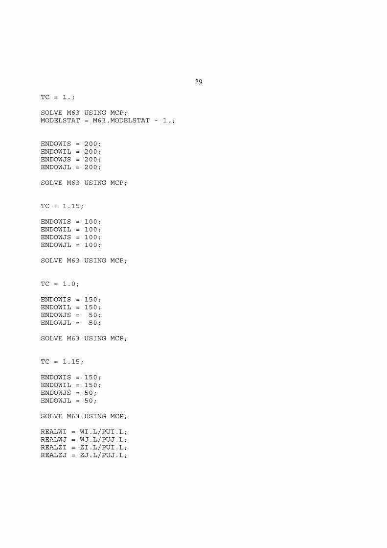
29

TC = 1.;


ENDOWIS = 200;ENDOWIL = 200;ENDOWJS = 200;ENDOWJL = 200;


TC = 1.15;



TC = 1.0;



TC = 1.15;




30






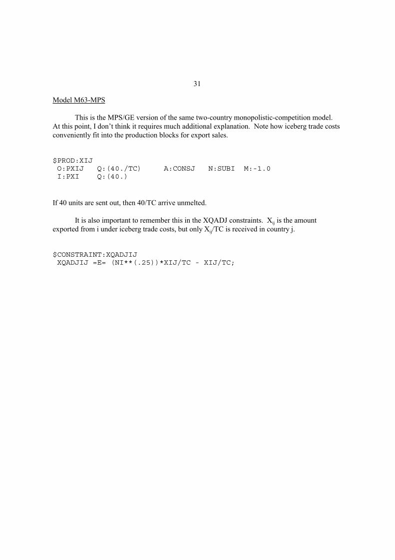
31

Model M63-MPS

This is the MPS/GE version of the same two-country monopolistic-competition model.

At this point, I don’t think it requires much additional explanation. Note how iceberg trade costs

conveniently fit into the production blocks for export sales.

$PROD:XIJ O:PXIJ Q:(40./TC) A:CONSJ N:SUBI M:-1.0 I:PXI Q:(40.)

If 40 units are sent out, then 40/TC arrive unmelted.

It is also important to remember this in the XQADJ constraints. Xij is the amount

exported from i under iceberg trade costs, but only Xij/TC is received in country j.

$CONSTRAINT:XQADJIJ XQADJIJ =E= (NI**(.25))*XIJ/TC - XIJ/TC;

32

$TITLE: Model M63: Two Country Large-Group Monopolistic Competition* uses MPS/GE

$ontext


PYI 100 -100PYJ 100 -100PXI 100 -50 -50PXJ 100 -50 -50FCI 20 -20FCJ 20 -20 ZI -40 -48 -12 100ZJ -40 -48 -12 100WI -60 -32 -8 100WJ -60 -32 -8 100UTILI 200 -200UTILJ 200 -200MKI -10 -10 10 10MKJ -10 -10 10 10

$offtext

PARAMETERS

ENDOWIL ENDOWJL ENDOWIS ENDOWJS TC SUBSIDY SIGMA REALWI REALWJ REALZI REALZJ;

ENDOWIL = 1.;ENDOWJL = 1.;ENDOWIS = 1.;ENDOWJS = 1.;TC = 1;SUBSIDY = 0;SIGMA = 5;

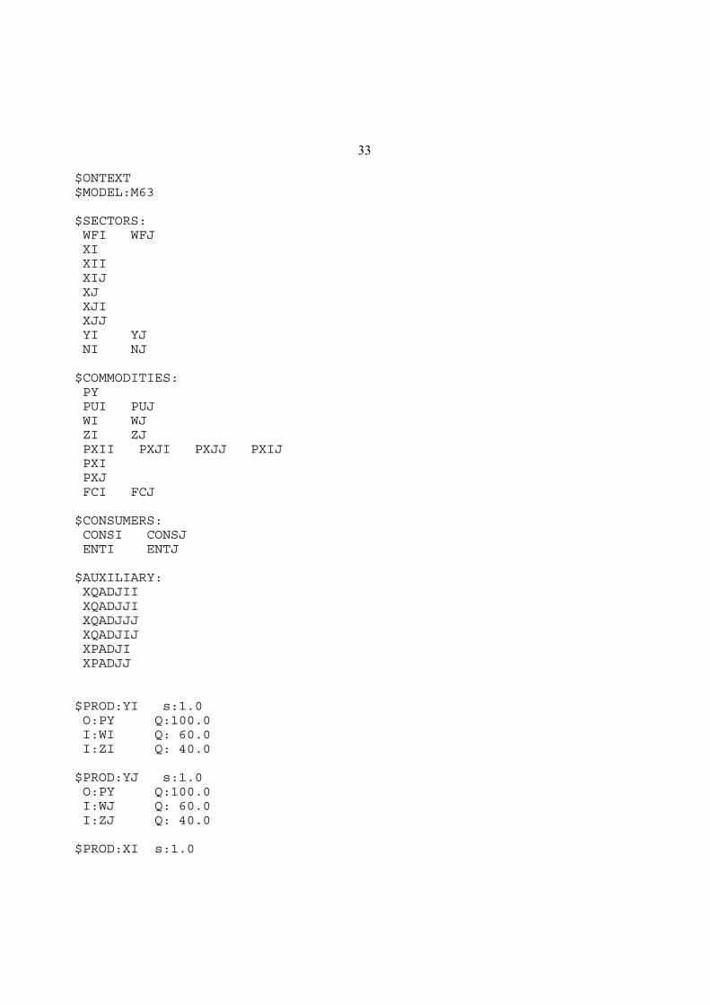
33

$ONTEXT$MODEL:M63

$SECTORS: WFI WFJ XI XII XIJ XJ XJI XJJ YI YJ NI NJ

$COMMODITIES: PY PUI PUJ WI WJ ZI ZJ PXII PXJI PXJJ PXIJ PXI PXJ FCI FCJ

$CONSUMERS: CONSI CONSJ ENTI ENTJ

$AUXILIARY: XQADJII XQADJJI XQADJJJ XQADJIJ XPADJI XPADJJ

$PROD:YI s:1.0 O:PY Q:100.0 I:WI Q: 60.0 I:ZI Q: 40.0

$PROD:YJ s:1.0 O:PY Q:100.0 I:WJ Q: 60.0 I:ZJ Q: 40.0

$PROD:XI s:1.0

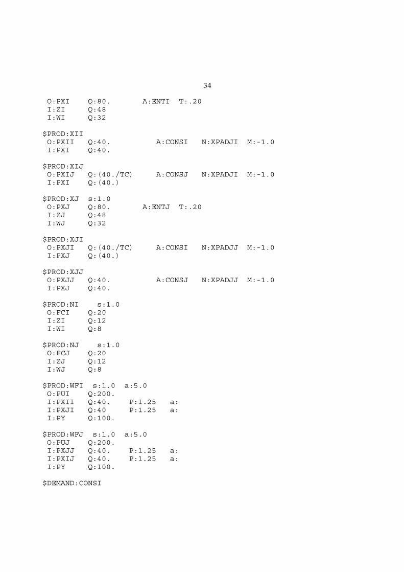
34

O:PXI Q:80. A:ENTI T:.20 I:ZI Q:48 I:WI Q:32

$PROD:XII O:PXII Q:40. A:CONSI N:XPADJI M:-1.0 I:PXI Q:40.

$PROD:XIJ O:PXIJ Q:(40./TC) A:CONSJ N:XPADJI M:-1.0 I:PXI Q:(40.)

$PROD:XJ s:1.0 O:PXJ Q:80. A:ENTJ T:.20 I:ZJ Q:48 I:WJ Q:32

$PROD:XJI O:PXJI Q:(40./TC) A:CONSI N:XPADJJ M:-1.0 I:PXJ Q:(40.)

$PROD:XJJ O:PXJJ Q:40. A:CONSJ N:XPADJJ M:-1.0 I:PXJ Q:40.

$PROD:NI s:1.0 O:FCI Q:20 I:ZI Q:12 I:WI Q:8

$PROD:NJ s:1.0 O:FCJ Q:20 I:ZJ Q:12 I:WJ Q:8

$PROD:WFI s:1.0 a:5.0 O:PUI Q:200. I:PXII Q:40. P:1.25 a: I:PXJI Q:40 P:1.25 a: I:PY Q:100.

$PROD:WFJ s:1.0 a:5.0 O:PUJ Q:200. I:PXJJ Q:40. P:1.25 a: I:PXIJ Q:40. P:1.25 a: I:PY Q:100.

$DEMAND:CONSI

35

D:PUI E:WI Q:(100*ENDOWIL) E:ZI Q:(100*ENDOWIS) E:PXII Q:40 R:XQADJII E:PXJI Q:40 R:XQADJJI

$DEMAND:CONSJ D:PUJ E:WJ Q:(100*ENDOWJL) E:ZJ Q:(100*ENDOWJS) E:PXIJ Q:40 R:XQADJIJ E:PXJJ Q:40 R:XQADJJJ

$DEMAND:ENTI D:FCI

$DEMAND:ENTJ D:FCJ

$CONSTRAINT:XQADJII XQADJII =E= (NI**(.25))*XII - XII;

$CONSTRAINT:XQADJJI XQADJJI =E= (NJ**(.25))*XJI/TC - XJI/TC;

$CONSTRAINT:XQADJJJ XQADJJJ =E= (NJ**(.25))*XJJ - XJJ;

$CONSTRAINT:XQADJIJ XQADJIJ =E= (NI**(.25))*XIJ/TC - XIJ/TC;

$CONSTRAINT:XPADJI XPADJI =E= NI**.25 - 1;

$CONSTRAINT:XPADJJ XPADJJ =E= NJ**.25 - 1;

$OFFTEXT$SYSINCLUDE MPSGESET M63

XQADJII.LO = -INF;XQADJIJ.LO = -INF;XQADJJI.LO = -INF;XQADJJJ.LO = -INF;

XPADJI.LO = -INF;XPADJJ.LO = -INF;

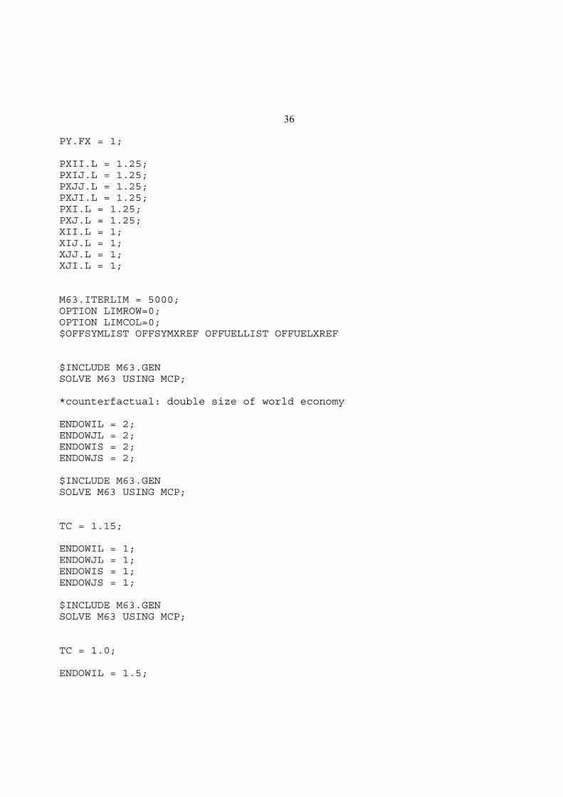
36

PY.FX = 1;

PXII.L = 1.25;PXIJ.L = 1.25;PXJJ.L = 1.25;PXJI.L = 1.25;PXI.L = 1.25;PXJ.L = 1.25;XII.L = 1;XIJ.L = 1;XJJ.L = 1;XJI.L = 1;

M63.ITERLIM = 5000;OPTION LIMROW=0;OPTION LIMCOL=0;$OFFSYMLIST OFFSYMXREF OFFUELLIST OFFUELXREF


*counterfactual: double size of world economy

ENDOWIL = 2;ENDOWJL = 2;ENDOWIS = 2;ENDOWJS = 2;


TC = 1.15;

ENDOWIL = 1;ENDOWJL = 1;ENDOWIS = 1;ENDOWJS = 1;


TC = 1.0;

ENDOWIL = 1.5;

37

ENDOWJL = .5;ENDOWIS = 1.5;ENDOWJS = .5;


TC = 1.15;

ENDOWIL = 1.5;ENDOWIS = 1.5;ENDOWJL = 0.5;ENDOWJS = 0.5;




ENDOWIL = 1.0;ENDOWIS = 1.2;ENDOWJL = 1.0;ENDOWJS = 0.8;




Chapter 1 General-Equilibrium Modeling using GAMS · PDF file1 Chapter 1 General-Equilibrium...

Documents

Transcript of Chapter 1 General-Equilibrium Modeling using GAMS · PDF file1 Chapter 1 General-Equilibrium...