Chapter 1

Fundamentals of Signal Decompositions

“A journey of a thousand miles must begin with a single step.” – Lao-Tzu,

Tao Te Ching

1.1 Functions and integration

Lebesgue integration: A function f is said to be integrable if

( )f t dt+∞

−∞< +∞∫ . The space of integrable functions is written

( )1L .

Two functions f1 and f2 are equal in ( )1L if

1 2( ) ( ) 0f t f t dt+∞

−∞− =∫ . We say that they are almost everywhere

equal.

Fatou Lemma: Let n nf ∈ be a family of positive functions

( ) 0nf t ≥ . If lim ( ) ( )nnf t f t

→+∞= almost everywhere then

( ) lim ( )nnf t dt f t dt

+∞ +∞

−∞ −∞→+∞≤∫ ∫ .

注：非负函数列在 Lebesgue积分下求极限的不等式。

Dominated Convergence Theorem: Let n nf ∈ be a family

such that lim ( ) ( )nnf t f t

→+∞= almost everywhere, If n∀ ∈ ,

( ) ( )nf t g t≤ and ( )g t dt+∞

−∞< +∞∫ , then f is integrable and

( ) lim ( )nnf t dt f t dt

+∞ +∞

−∞ −∞→+∞=∫ ∫ .

注：函数族存在一个可积函数作为上界条件下，在 Lebesgue

积分下取极限的等式。

Fubini Theorem: If 1 2 1 2( ( , ) )f x x dx dx+∞ +∞

−∞ −∞< +∞∫ ∫

then1 2 1 2 1 2 1 2

1 2 2 1

( , ) ( ( , ) )

( ( , ) )

f x x dx dx f x x dx dx

f x x dx dx

+∞ +∞ +∞ +∞

−∞ −∞ −∞ −∞

+∞ +∞

−∞ −∞

=

=

∫ ∫ ∫ ∫∫ ∫

Note: It is a sufficient condition for inverting the order of

integrals in multidimensional integrations.

Convexity: A function ( )f t is said to be convex if for all

1 2, 0p p > with 1 2 1p p+ = and all 21 2( , )t t ∈ ,

1 1 2 2 1 1 2 2( ) ( ) ( )f p t p t p f t p f t+ ≤ + .

Note:

(1) The function f satisfies the reverse inequality and is said to be

concave.

(2) If f is convex then the Jesen inequality generalizes the

property: For any 0kp ≥ with 1

1K

kk

p=

=∑ and any kt ∈ ,

1 1

( ) ( )K K

k k k kk k

f p t p f t= =

≤∑ ∑ .

Proposition (命题) 2.1: If f is twice differentiable, then f is

convex if and only if "( ) 0f t ≥ for all t∈ . （单调递增）

Note: The notion of convexity also applies to sets nΩ⊂ . This

set is convex if for all 1 2, 0p p > with 1 2 1p p+ = and all

21 2( , )x x ∈Ω , 1 1 2 2p x p x+ ∈Ω . If Ω is not convex then its convex

hull is defined as the smallest convex set that includes Ω .

1.2 Banach and Hilbert Spaces

Note: Signals are often considered as vectors.

Banach space (完备的距离空间): To define a distance, let us

consider a vector space H that admits a norm, which satisfies

the following properties: f∀ ∈H , 0f ≥ and

0 0f f= ⇔ = ;

λ∀ ∈ , f fλ λ= ;

,f g∀ ∈H , f g f g+ ≤ + .

(1) With such a norm, the convergence of n nf ∈ to f in H

means that lim lim 0n nn nf f f f

→+∞ →+∞= ⇔ − = .

(2) To guarantee the limits remaining in H, a completeness （完

备性）property is imposed, with the notion of Cauchy

sequences: A sequence n nf ∈ is a Cauchy sequence if for

any 0ε > , if n and p are larger enough, then n pf f ε− < .

The space H is said to be complete if every Cauchy sequence

in H converges to an element of H.

Example:

(1) : p

f f= < +∞p1 is a Banach space with the norm p

f

where 1

[ ]p

p

pn

f f n+∞

=−∞

⎛ ⎞= ⎜ ⎟⎝ ⎠∑ for any integer 0p ≥ .

(2) ( )pL is a Banach space which is composed of the

measurable functions f on with the norm 1

( )p p

pf f t dt

+∞

−∞

⎛ ⎞= < +∞⎜ ⎟⎝ ⎠∫

Hilbert Space: A Banach space with an inner product.

(1) The inner product of two vectors ,f g is linear with

respect to its first argument (第一个向量 ): 1 2,λ λ∀ ∈ ，

1 1 2 2 1 1 2 2, , ,f f g f g f gλ λ λ λ+ = + .

(2) Hermitian symmetry: *, ,f g g f= .

(3) , 0f f ≥ and , 0 0f f f= ⇔ = .

Note: 1/ 2,f f f= is a norm.

Example:

(1) An inner product between discrete signals [ ]f n and [ ]g n

can be defined by *, [ ] [ ]f g f n g n+∞

−∞

=∑ . It corresponds to an ( )21

norm: 2 2, [ ]f f f f n+∞

−∞

= =∑ . The space ( )21 of finite energy

sequences is therefore a Hilbert space.

(2) Over analog signals ( )f t and ( )g t , an inner product can be

defined by *, ( ) ( )f g f t g t dt+∞

−∞= ∫ . The resulting norm is

( )2 2( )f f t dt+∞

−∞= ∫ . The space ( )2L of finite energy functions is

thus also a Hilbert space.

(3) Cauchy-Schwarz inequality: ,f g f g≤ , which is an

equality if and only if f and g are linearly dependent. 1/ 2 1/ 2

2 2*[ ] [ ] [ ] [ ]n n n

f n g n f n g n+∞ +∞ +∞

=−∞ =−∞ =−∞

⎛ ⎞ ⎛ ⎞≤ ⎜ ⎟ ⎜ ⎟⎝ ⎠ ⎝ ⎠

∑ ∑ ∑

( ) ( )1/ 2 1/ 22 2*( ) ( ) ( ) ( )f t g t dt f t dt g t dt

+∞ +∞ +∞

−∞ −∞ −∞≤∫ ∫ ∫

Proof: * 2

22 2 * *

0 [ ( ) ( )]

( ) 2 ( ) ( ) ( )

b

a

b b b

a a a

f t g t dt

f t dt f t g t dt g t dt

λ

λ λ

≤ −

= − +

∫∫ ∫ ∫

∵

* 2

22 2 * *

0 [ ( ) ( )]

[ ] 2 [ ] [ ] [ ]

b

n a

b b b

n a n a n a

f n g n

f n f n g n g n

λ

λ λ

=

= = =

≤ −

= − +

∑

∑ ∑ ∑

∵

(4) The notions of norm and orthogonality can be expressed to

functions using a suitable inner product between functions, which

are thus viewed as vectors. A classic example of such orthogonal

vectors is the set of harmonic sine and cosine functions, sin(nt) and

cos(nt), n=0,1,⋯,on the interval [ , ]π π− .

1.3 Bases of Hilbert Spaces

Orthogonal: For the standard inner product in 3 , the law of

cosine is , cos( )f g f g θ= , which implies that f and g are

orthogonal (perpendicular) if and only if , 0f g =

Orthonormal Basis: A family n ne ∈ of a Hilbert space H is

orthogonal if for n p≠ , , 0n pe e = .

If for f ∈H there exists a sequence [ ]nλ such that

0

lim [ ] 0N

nx n

f n eλ→∞

=

− =∑ , then n ne ∈ is said to be an orthononal

basis of H. The orthogonality implies that necessarily

2

,[ ] n

n

f en

eλ = and we write 2

0

, nn

n n

f ef e

e

+∞

=

=∑ .

(1) A Hilbert space that admits an orthogonal basis is said to be

separable.

(2) The basis is orthonormal if 1ne = for all n∈ . Therefore,

we can obtain a Parseval equation for orthonormal bases:

*

0

, , ,n nn

f g f e g e+∞

=

=∑

When g f= , we get an energy conservation called the

Plancherel formula: 22

0

, nn

f f e+∞

=

=∑ . (请注意)

(3) The Hilbert spaces ( )21 and ( )2L are separable. For

example, the family of translated Diracs [ ] [ ]n ne k k nδ

∈= − is

an orthonormal basis of ( )21 .

Riesz Bases: In an infinite dimensional space, if we loosen up

the orthonality requirement, we must still impose a partial

energy equivalence to guarantee the stability of the basis. A

family of vectors n ne ∈ is said to be a Riesz basis of H if it

is linearly independent and there exist 0A > and 0B > such

that for any f ∈H one can find [ ]nλ with 0

[ ] nn

f n eλ+∞

=

=∑ ,

which satisfies 2 2 21 1[ ]n

f n fB A

λ≤ ≤∑ .

(1) The Riesz representation theorem proves that there exist ne

such that [ ] , nn f eλ = , so 22 21 1, nn

f f e fB A

≤ ≤∑ .

Theorem: Let n nφ ∈ be a frame with bounds A, B, the dual

frame defined by * 1( )n nU Uφ φ−= satisfies:

f∀ ∈H , 22 21 1, n

n

f f fB A

φ≤ ≤∑ , and

1 , ,n n n nn n

f U Uf f fφ φ φ φ−

∈Γ ∈Γ

= = =∑ ∑

Note: The dual family of vectors n nφ ∈ and n nφ ∈ play

symmetrical roles, it implies:

, , ,n nn

f g f gφ φ∈Γ

=∑ , so , n nn

g g φ φ∈Γ

=∑ ;

Thus: for all f ∈H , we can derives that

22 2, nn

A f f e B f∈Γ

≤ ≤∑ and

0 0

, ,n n n nn n

f f e e f e e+∞ +∞

= =

= =∑ ∑

(2) The dual family n ne ∈ is linearly independent and is also a

Riesz basis. The case pf e= yields 0

,p p n nn

e e e e+∞

=

=∑ . The linear

independence of n ne ∈ thus implies a biorthogonality

relationship between dual bases, which are called biorthogonal

bases: , [ ]n pe e n pδ= − .

1.4 Linear Operators

An operator T from a Hilbert space H1 to another Hilbert H2 is linear

if 1 2 1 2, , , ,f fλ λ∀ ∈ ∀ ∈H 1 1 2 2 1 1 2 2( ) ( ) ( )T f f T f T fλ λ λ λ+ = + .

Sup Norm: The sup operator norm of T is defined by

1

supS

f

TfT

f∈=

H. If this norm is finite, then T is continuous.

Tf Tg− becomes arbitrarily small if f g− is sufficiently

small.

Adjoint: The adjoint of T is the operator T* from H2 to H1

such that for any 1f ∈H and 2g∈H , *, ,Tf g f T g= .

When T is defined from H into itself, it is self-adjoint if

*T T= .

(1) A non-zero vector f ∈H is called an eigenvector if there

exists an eigenvalue λ∈ such that Tf fλ= .

(2) In a finite dimensional Hilbert space (Euclidean space), a

self-adjoint operator is always diagonalized by an orthogonal

basis 0n n Ne

≤ ≤ of eigenvectors n n nTe eλ= .

(3) When T is self-adjoint the eigenvalues nλ are real. For any

f ∈H , 1 1

0 0

, ,N N

n n n n nn n

Tf Tf e e f e eλ− −

= =

= =∑ ∑

Orthogonal Projector: Let V be a subspace of H. A projector

PV on V is a linear operator that satisfies

f∀ ∈H , P f ∈V V and f∀ ∈V , P f f=V .

The projector is orthogonal if f∀ ∈H , g∀ ∈V ,

, 0f P f g− =V .

(1) Proposition: If PV is a projector on V then the following

statements are equilavent:

PV is orthogonal.

PV is self-adjoint.

1S

P =V

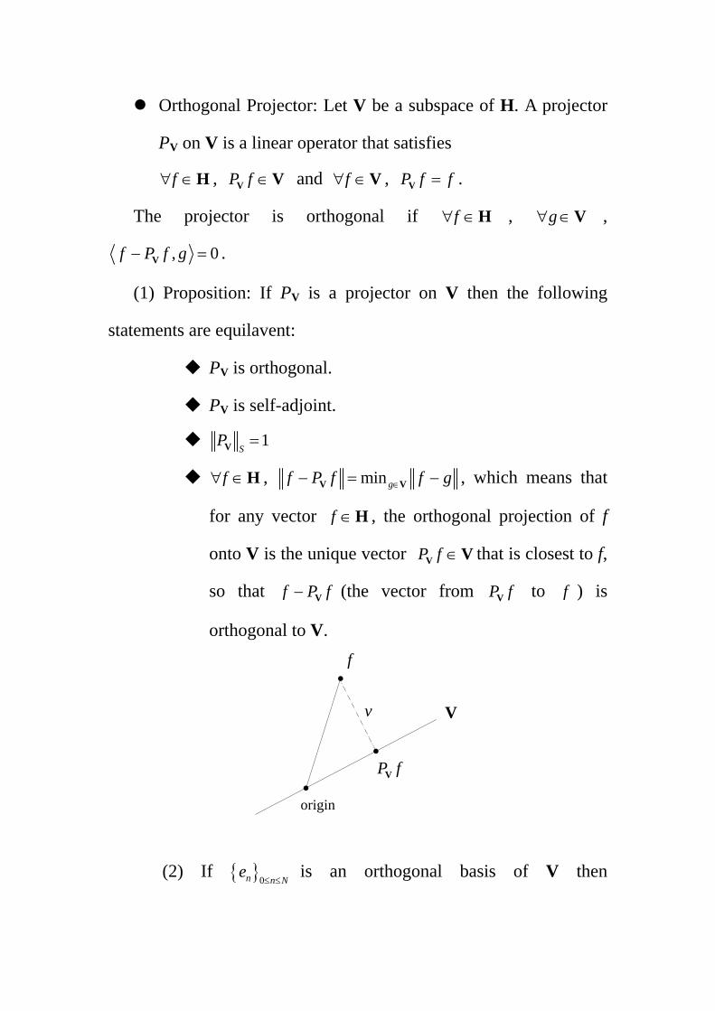
f∀ ∈H , min gf P f f g∈− = −V V , which means that

for any vector f ∈H , the orthogonal projection of f

onto V is the unique vector P f ∈V V that is closest to f,

so that f P f− V (the vector from P fV to f ) is

orthogonal to V.

V

f

P fV

origin

v

(2) If 0n n Ne

≤ ≤is an orthogonal basis of V then

20

, nn

n n

f eP f e

e

+∞

=

=∑V .

If 0n n Ne

≤ ≤ is a Riesz basis of V and 0n n N

e≤ ≤

is the

biorthogonal basis then 0 0

, ,n n n nn n

P f f e e f e e+∞ +∞

= =

= =∑ ∑V .

(3) Each vector f∀ ∈H can be written uniquely as

f P f v= +V , where v belongs to ; , , 0v g v g⊥ = ∈ ∀ ∈ =V H V

and P f ∈V V .

参注：

(1) 《信号与系统》教材中的相应说明：类似于矢量分解，信

号的分量及其分解即为函数的分量及其分解，

1 12 2( ) ( ) ( )t f t c f tε∆ = −

2

1

21 12 2

12

[ ( ) ( )] 0t

tf t c f t dt

cδδ

− =∫

2

1

2

1

*1 2

12 *2 2

( ) ( )

( ) ( )

t

tt

t

f t f t dtc

f t f t dt=∫∫

(2) 从功率角度出发，相关系数（二分量系数的几何中值）：

2

1

2

1

2 2

1 1

12

2min

12*

2 22 1

*1 2

12 2112* *

1 1 2 2

( )1 1 ( ) ( )

( ) ( )

( ) ( ) ( ) ( )

t

t

t

t

t t

t t

tcf t f t dt

t t

f t f t dtc c

f t f t dt f t f t dt

ε∆⎡ ⎤⎢ ⎥⎢ ⎥= −⎢ ⎥⎢ ⎥−⎣ ⎦

= =⎡ ⎤⎢ ⎥⎣ ⎦

∫

∫

∫ ∫

(3) 三角傅里叶级数（周期为 2T π=Ω的周期信号）：

0 0

1 1( ) ( cos sin ) cos( )

2 2n n n nn n

a af t a n t b n t A n t ϕ∞ ∞

= =

= + Ω + Ω = + Ω −∑ ∑

1 1

1 1

00

1 2( ) ( ) , ( )2

t T t T

t t

af t f t dt a f t dtT T

+ += = =∫ ∫

1

11

1 1

1

2

( ) cos 2 ( )coscos

t T

t Ttn t T t

t

f t n tdta f t n tdt

Tn tdt

+

+

+

Ω= = Ω

Ω

∫∫

∫

1

11

1 1

1

2

( )sin 2 ( )sinsin

t T

t Ttn t T t

t

f t n tdtb f t n tdt

Tn tdt

+

+

+

Ω= = Ω

Ω

∫∫

∫

2 2n n nA a b= + ， n

nn

barctga

ϕ = ， cosn n na A ϕ= ， sinn n nb A ϕ=

因为： 1 1

1 1

2 2cos sin2

t T t T

t t

Tn tdt n tdt+ +

Ω = Ω =∫ ∫ 1 1

1 1

cos cos sin sin 0t T t T

t tm t n tdt m t n tdt

+ +Ω Ω = Ω Ω =∫ ∫ ，m n≠

1

1

sin cos 0t T

tm t n tdt

+Ω Ω =∫ ， ,m n∀

(4) 指数傅里叶级数：

1( )2

in t in tn n

n nf t c e A e

∞ ∞Ω Ω

=−∞ =−∞

= =∑ ∑ ，

1

11

1 1

1

( ) 1 ( )

t T in tt Tt in t

n t T tin t in t

t

f t e dtc f t e dt

Te e dt

+ − Ω+ − Ω

+ Ω − Ω= =∫

∫∫

，

2nin n nA A e cϕ−= =

(5) Gibbs现象：

对于具有不连续点的函数，即使所取级数的项数无限增大，

在不连续处，级数之和仍不收敛于函数，在跃变点附近波形，总

是不可避免存在起伏振荡，从而使跃变点附件某些点形成过冲。

(6) 周期矩形脉冲（A 为脉冲幅度， ( , )2 2τ ττ − 为脉冲宽度，T

为脉冲重复周期）

2 sin / 2 2 sin // 2 /n

A n A n TAT n T n Tτ τ τ πτ

τ πτΩ⎡ ⎤ ⎡ ⎤= =⎢ ⎥ ⎢ ⎥Ω⎣ ⎦ ⎣ ⎦

， 0

2a A

Tτ

=

sin / 2( )/ 2

jn t

n

A nf t eT nτ τ

τ

∞Ω

=−∞

Ω=

Ω∑

(7) 周期信号频谱特性：

离散性：频谱由不连续线条（正弦分量）组成；

谐波形：每条谱线都只能出现在基波频率Ω的整数倍频率

上；

收敛性：各条谱线的高度，即各次谐波的振幅，总的趋势是

随着谐波次数的增高而逐渐减小。

周期增大，信号频谱趋密集，频谱幅度相应趋小；

脉冲宽度减小，频谱振幅收敛速度相应变慢（即信号频宽加

大，一切脉冲信号的脉宽与频宽成反比），频谱振幅相应减小；

注：一般频谱，其频带宽度定义为，从零频率开始到频谱振

幅降为包络线最大值的1

10的频率间频带。

(8) 非周期信号频谱：

2

2

2 ( )T

in tTnA f t e dt

T− Ω

−= ∫∵

2

2

ˆ ( ) lim lim ( ) ( )2

Tin t i tn

TT T

TAf f t e dt f t e dtωω∞− Ω −

−∞→∞ →∞ −= = =∫ ∫

2

2

1 1 2( ) ( )2 2

Tin t in t in t

Tnn n

f t A e f t e dt eT

∞ ∞Ω − Ω Ω

−=−∞ =−∞

⎡ ⎤= = ⎢ ⎥

⎣ ⎦∑ ∑ ∫

2 2, ,d n Td

π πω ωω

Ω→ Ω→ = →Ω

∵ 1 ˆ( ) ( )

2i tf t f e dωω ω

π∞

−∞= ∫

如：

1．矩形脉冲频谱（门函数 ( ), ( , )2 2

G tττ τ

− ，A为脉冲幅度）： 2ˆ( ) ( ) ( ) ( ) sin ( )

2 2 2 2AG t u t u t f A Saτ

τ τ ωτ ωτω τω

= + − − ↔ = =

抽样函数sin / 2 2( ) ( ) ( ) ( )

2 / 2 2 2t tSa G u u

tπω ω ωΩ

Ω Ω Ω Ω⎡ ⎤= ↔ = + − −⎢ ⎥Ω Ω ⎣ ⎦

2．单边指数信号 1( )ate u ta iω

− ↔+

3．双边指数信号 2 2

2a t aea ω

− ↔+

4． ( ) 1tδ ↔ ， 21( ) ( )i

u t eπ

πδ ωω

−↔ + ，

2sgn( )tiω

↔

5． 2 ( )ci tce ω πδ ω ω↔ − ，1 2 ( )πδ ω↔ ，

cos [ ( ) ( )]c c ctω π δ ω ω δ ω ω↔ + + −

sin [ ( ) ( )]c c ct iω π δ ω ω δ ω ω↔ + − −

6． ( ) ( )Tn

t t nTδ δ∞

=−∞

= −∑

1ˆ ( ) ( ) ( )2

2 ( ) ( )

in tn n

n n

n

f Lf t L A e A n

nT

ω π δ ω

π δ ω δ ω

∞ ∞Ω

=−∞ =−∞

∞

Ω=−∞

⎧ ⎫↔ = = = − Ω⎨ ⎬

⎩ ⎭

= − Ω = Ω

∑ ∑

∑

注：一个冲激序列的傅里叶变换仍是一冲激序列。

注：非周期性脉冲信号的频谱函数 ˆ ( )f ω ，和由该脉冲按一定

周期2T π

=Ω重复后所构成的周期信号的复数振幅 nA 之间，只要知

道一个，另一个就可以由 n ωΩ→ 及乘以或除以2T获得。

Limit and Density Argument: Let n nT

∈ be a sequence of

linear operators from H to H. Such a sequence converges

weakly to a linear operator T∞ if f∀ ∈H , lim 0nmT f T f∞→∞

− = .

(1) To find the limit of operators it is often preferable to work in

a well chosen subspace ⊂V H which is dense. A space V is

dense in H if for any f ∈H there exist m mf

∈ with

mf ∈V such that lim 0mmf f

→∞− = .

Proposition (Density): Let V be a dense subspace of H. Suppose

that there exists C such that n ST C≤ for all n∈ . If

f∀ ∈V , lim 0nnT f T f∞→∞

− = , then

f∀ ∈H , lim 0nnT f T f∞→∞

− = .

1.5 Separable Spaces and Bases

Tensor Product: Tensor products are used to extend spaces of

one-dimensional signals into spaces of multiple dimensional

signals. A tensor product 1 2f f⊗ between vectors of two

Hilbert spaces H1 and H2 satisfies the following properties:

Linearity: λ∀ ∈ , 1 2 1 2 1 2( ) ( ) ( ) ( )f f f f f fλ λ λ⊗ = ⊗ = ⊗

Distributivity:

1 1 2 2 1 2 1 2 1 2 1 2( ) ( ) ( ) ( ) ( ) ( )f g f g f f f g g f g g+ ⊗ + = ⊗ + ⊗ + ⊗ + ⊗

This tensor product yields a new Hilbert space 1 2= ⊗H H H that

includes all vectors of the form 1 2f f⊗ where 1 1f ∈H and 2 2f ∈H ,

as well as linear combinations of such vectors. An inner product in

H is derived from inner products in H1 and H2 by

1 21 2 1 2 1 1 2 2, , ,f f g g f g f g⊗ ⊗ =

H H H

Separable Bases:

Theorem: Let 1 2= ⊗H H H . If 1n n

e∈

and 2n n

e∈

are two

Riesz bases respectively of H1 and H2 then 2

1 2

( , )n n n me e

∈⊗ is a

Riesz basis of H. If the two bases are orthonormal then the tensor

product basis is also orthonormal.

The theorem proves that orthogonal bases of tensor product

spaces are obtained with separable products of two orthonormal

bases. It provides a simple procedure for transforming bases for

one-dimensional signals into separable bases for multidimensional

signals.

Example:

(1) Let 2( )2L be the space of 1 2( , )h x x such that 2

1 2 1 2( , )h x x dx x+∞ +∞

−∞ −∞< +∞∫ ∫ . A product of functions ( )f ∈ 2L

and ( )g∈ 2L defines a tensor product:

1 2 1 2( ) ( ) ( , )f x g x f g x x= ⊗ . One can verify that

2( ) ( ) ( )= ⊗2 2 2L L L

(2) ( )f ∈ 21 and ( )g∈ 21 also defines a tensor product:

1 2 1 2[ ] [ ] [ , ]f n g n f g n n= ⊗ . The space 2( )21 of images

1 2( , )h n n such that 1 2

21 2[ , ]

n n

h n n+∞ +∞

=−∞ =−∞

< +∞∑ ∑ is also

decomposed as a tensor product 2( ) ( ) ( )= ⊗2 2 21 1 1 .

Orthonormal bases can thus be constructed with separable

products.

1.6 Random Vectors and Covariance Operators

A class of signals can be modeled by a random process (random

vector) whose realizations are the signals in the class. Finite discrete

signals f are represented by a random vector Y, where Y[n] is a

random variable for each 0 n N≤ ≤ .

Covariance Operator: The average of a random variable X is

E X . The covariance of two random variables 1X and 2X

is *1 2 1 1 1 2( , ) ( )( ) Cov X X E X E X X E X= − − .

(1) The covariance matrix of a random vector Y is composed of

the N2 covariance values [ , ] ( [ ], [ ])R n m Cov Y n Y m= . It defines the

covariance operator K which transforms any h[n] into 1

0

[ ] [ , ] [ ]N

m

Kh n R n m h m−

=

=∑ .

Note:

(2) For any h and g, 1

*

0

, [ ] [ ]N

n

Y h Y n h n−

=

=∑ and

1*

0

, [ ] [ ]N

n

Y g Y n g n−

=

=∑ are random variables and

( ), , , ,Cov Y h Y g Kg h=

Note:

The covariance operator thus specifies the covariance

of linear combinations of the process values.

The covariance operator K is self-adjoint because *[ , ] [ , ]R n m R m n= and positive because

2, , 0Kh h E Y h= ≥ .

Karhunen-Loève Basis: Because a self-adjoint operator is

always diagonalized by an orthogonal basis 0k k Ng

≤ ≤ of

eigenvectors 2k k kKg gσ= (owing to the positive operator),

where 22 , ,k k k kKg g E Y gσ = = , this basis is called a

Karhunen-Loève basis of Y, and the vectors gk are the

principle directions.

Wide-Sense Stationarity (宽平稳性 ): We say that Y is

wide-sense stationarity if *[ ] [ ] [ , ] [ ]YE Y n Y m R n m R n m= = − .

(1) The correlation at two points depends only on the distance

between these points. The operator K is then a convolution whose

kernel [ ]YR k is defined for N k N− < < .

(2) A wide-sense stationary process is circular stationary if [ ]YR n

is N periodic: [ ] [ ]Y YR n R N n= + for 0N n− < < . This condition

implies that a periodic extension of Y[n] on Z remains wide-sense

stationary on Z .

(3) The covariance operator K of a circular stationary process is a

discrete circular convolution. The eigenvectors of circular

convolutions are the discrete Fourier vectors

0

1 2[ ] expkk N

i kng nNNπ

≤ ≤

⎧ ⎫⎛ ⎞=⎨ ⎬⎜ ⎟⎝ ⎠⎩ ⎭

. Therefore, the discrete Fourier basis

is the Karhunen-Loève basis of circular stationary processes. 1

0

2 2[ ] exp [ ]expN

k Yp

i kn i kpKg n R pN Nπ π−

=

−⎛ ⎞ ⎛ ⎞= ⎜ ⎟ ⎜ ⎟⎝ ⎠ ⎝ ⎠

∑∵

Thus, the eigenvalues of K are the discrete Fourier transform of

RY and are called the power spectrum 1

2

0

2ˆ [ ] [ ]expN

k Y Yn

i k nR k R nNπσ

−

=

−⎛ ⎞= = ⎜ ⎟⎝ ⎠

∑ .

Theorem: Let Z be a wide-sense circular stationary random

vector. The random vector [ ] [ ]Y n Z h n= (circular convolution) is

also wide-sense circular stationary and its power spectrum is 2ˆ[ ] [ ] [ ]Y ZR k R k h k=

1.7 Vector Spaces and Inner Products

A vector space over the set of complex or real numbers, or ,

is a set vectors, E, together with addition and scalar multiplication,which,

for general x, y in E, andα ,β in or , satisfy the following:

(a) Commutativity: xyyx +=+

(b) Associativity: )()(),()( xxzyxzyx βααβ =++=++

(c) Distributivity: xxxyxyx βαβαααα +=++=+ )(,)(

(d) Additive identity: there exists 0 in E, such that xx =+ 0 , for all

x in E.

(e) Additive inverse: for all x in E, there exists a )( x− in E, such

that 0)( =−+ xx

(f) Multiplication identity: xx =⋅1 for all x in E.

Often, x, y in E will be n-tuples or sequences, and then we define

( ) ( ) ( ),,,,,, 22112121 yxyxyyxxyx ++=+=+

( ) ( ),,,, 2121 xxxxx αααα ==

While the scalars are from or , the vectors can be arbitrary, and

apart from n-tuples and infinite sequences, we could also take functions

over the real line.

A subset M of E is a subsequence of E if

(a) for all x and y in M, yx + is in M.

(b) for all x in M andα in or , xα is in M.

Given ES ⊂ , the span of S is the subspace of E consisting of all linear

combinations of vectors in S, for example, in finite dimensions,

⎭⎬⎫

⎩⎨⎧ ∈∈= ∑

=

SS ii

n

iii xRorCxspan , |)(

1αα

Vectors nxxx ,, 21 are called linearly independent, if 01

=∑=

n

iii xα is true

only if 0=iα , for all i. Otherwise, these vectors are linearly dependent. If

there are infinitely many vectors ,, 21 xx , they are linearly independent

if for each k, kxxx ,, 21 are linearly independent.

A subset ,, 21 nxxx of a vector space E is called a basis for E,

when and are linearly independent. Then, we say that E has dimension n.

E is infinite-dimensional if it contains an infinite linearly independent set

of vectors. As an example, the space of infinite sequences is spanned by

the infinite set. Since they are linearly independent, the space is

infinite-dimensional.

An inner product on a vector space E over or , is a

complex-valued function ⋅⋅, , defined on EE× with the following

properties:

(a) , , ,x y z x z y z+ = +

(b) , ,x y x yα α=

(c) *, ,x y y x=

Note that *, ,x y x yα α=

(d) , 0,x x ≥ and , 0x x = if and only if 0x ≡

For illustration, the standard inner product for complex-valued

functions over and sequences over are:

*, ( ) ( )f g f t g t dt∞

−∞= ∫ and *, [ ] [ ]

n

x y x n y n∞

=−∞

= ∑

The norm of a vector is defined from the inner product as

,x x x= , and ( )1/

( )p

p

pf f t dt

∞

−∞= ∫

The following hold for inner products over a vector space:

(a) Cauchy-Schwarz inequality: ,x y x y≤ , with equality if

and only if x yα=

(b) Triangle inequality: x y x y+ ≤ + with equality if and only

if x yα= , where α is a positive real constant.

(c) Parallelgram (毕达哥拉斯) law: ( )2 2 2 22x y x y x y+ + − = +

The inner product can be used to define orthogonality of two vectors

x and y , that is, two vectors x and y are orthogonal if and only if

, 0x y = .

If two vectors are orthogonal, which is denoted by x y⊥ , then they

satisfy the Pythagorean theorem: 2 2 2x y x y+ = + , since

2 2 2, , ,x y x y x y x x y y x y+ = + + = + + + .

A vector x is said to be orthogonal to a set of vectors iS y= if

, 0ix y = for all i. We denote this by x S⊥ . More generally, two

subspaces 1S and 2S are called orthogonal if all vectors in 1S are

orthogonal to all of the vectors in 2S , and this is written 1 2S S⊥ . A set of

vectors 1 2, ,x x is called orthogonal if i jx x⊥ when i j≠ . If the

vectors are normalized to have unit norm, we have an orthonormal system,

which therefore satisfies: , [ ]i jx x i jδ= − . Vectors in an orthonormal

system are linearly independent, since 0i ixα =∑ implies

0 , ,j i i i j i jx x x xα α α= = =∑ ∑ . An orthonormal system in a vector space

E is an orthonormal basis if it spans E.

1.8 Hilbert Space (Complement)

A complete inner product space is called a Hilbert space.

A Hilbert space contains a countable orthonormal basis if and only if

it is separable. A closed subspace of a separable Hilbert space is separable,

that is, it also contains a countable orthonormal basis.

Given a Hilbert space E and a subspace S, we call the orthogonal

complement of S in E, denoted ⊥S , the set SE ⊥∈ xx | . Assume

further that S is closed, that is, it contains all limits of sequences of

vectors in S. Then, given a vector y in E, there exists a unique v in S

and a unique w in ⊥S such that wvy += . We can thus write

⊥⊕= SSE , or, E is the direct sum of the subspace and its orthogonal

complement.

Complex/Real Spaces:

The complex space n is the set of all n-tuples ( )0 1, , , nx x x=x ,

with finite ix in . The inner product is defined as Z

∑=

=n

iii yxyx

1

*,

and the norm is : ∑=

==n

iixxxx

1

2,

Space of Square-Summable Sequences:

In discrete-time signal processing we will be dealing almost

exclusively with sequences ][nx having finite square sum or finite

energy, where ][nx is, in general, complex-valued and n belongs to Z .

Such a sequence ][nx is a vector in the Hilbert space ( )21 . The inner

product is: ∑∞

−∞=

=n

nynxyx ][][, *

and the norm is: ∑∈

==Zn

nxxxx 2][,

( )21 is the space of all sequences such that x < ∞ . This is

obviously an infinite-dimensional space, and a possible orthonormal basis

is [ ]k

n kδ∈

− .

For the completeness of ( )21 , one has to show that if [ ]nx k is a

sequence of vectors in ( )21 such that 0n mx x− → as ,n m →∞ (that

is, a Cauchy sequence), then there exists a limit x in ( )21 such that

0nx x− → .

Space of Square-Integrable Functions

A function ( )f t defined on is said to be in the Hilbert space

( )2L , if 2( )f t is integrable (Lebesgus integrable), that is, if

2( )t

f t dt∈

< ∞∫ .

The inner product on ( )2L is given by *, ( ) ( )t

f g f t g t dt∈

= ∫ ,

and the norm is 2, ( )t

f f f f t dt∈

= = ∫ .

This space is infinite-dimensional (for example, 2 2 22, , ,t t te te t e− − −

are linearly independent).

1.9 Orthonormal Bases

Gram-Schmidt orthogonalization

Given a set of linearly independent vectors ix in E, we can

construct an orthonormal set iy with the same span as ix as

follows: Start with

11

1

xyx

=

then, recursively set k kk

k k

x vyx v−

=−

, 2,3,k =

where 1

1,

k

k i k ii

v y x y−

=

= ∑ .

As will be seen shortly, the vector kv is the orthogonal projection of

kx onto the subspace spanned by the previous orthogonalized

vectors and this is subtracted from kx , followed by normalization.

A standard example of such an orthogonalization procedure is

the legendre polynomials over the interval [ 1,1]− . Start with ( ) kkx t t= ,

0,1,k = and apply the Gram-Schmidt procedure to get ( )ky t , of

degree k, norm 1 and orthogonal to ( ),iy t i k<

Bessel’s Inequality

If we have an orthonormal system of vectors kx in E, then

for every y in E the following inequality, known as Bessel’s

inequality, holds: 22 ,kk

y x y≥∑ .

If we have an orthonormal system that is complete in E, then we

have an orthonormal basis for E, and Bessel’s relation becomes an

equality, often called Parseval’s equality.

Orthonormal Bases

For a set of vectors iS x= to be an orthonormal basis, we first

have to check that the set of vectors S is orthonormal and then that it

is complete, that is, that every vector from the space to be

represented can be expressed as a linear combination of the vectors

from S. In other words, an orthonormal system ix is called an

orthonormal basis for E, if for every y in E, k kk

y xα=∑ .

The coefficients kα of the expansion are called the Fourier

coefficients of y (with respect to ix ) and are given by ,k kx yα = .

This can be shown by using the continuity of the inner product (that

is, if nx x→ , and ny y→ , then , ,n nx y x y→ ) as well as the

orthogonality of the 'kx s .

0

, lim ,n

k k i i kn i

x y x xα α→∞

=

= =∑

where we used the linearity of the inner product.

The following theorem gives several equivalent statements

which permit us to check if an orhonormal system is also a basis:

Theorem: Given an orthonormal system 1 2, ,x x in E, the

following are equivalent:

(a) The set of vectors 1 2, ,x x is an orthonormal basis for E.

(b) If , 0ix y = for 1,2,i = , then 0y = .

(c) ( )ispan x is dense in E, that is, every vector in E is a limit

of a sequence of vectors in ( )ispan x .

(d) For every y in E, 22 ,ii

y x y=∑ , which is called Parseval’s

equality.

(e) For every y1 and y2 in E, *1 2 1 2, , ,i i

iy y x y x y=∑ , which is

often called the generalized Parseval’s equality.

Orthogonal Projection and Least-Squares Approximation

A vector from a Hilbert space E has to be approximated by a

vector lying in a (closed) subspace S. We assume that E is separable,

thus, S contains an orthonormal basis 1 2, ,x x . Then, the

orthogonal projection of y∈E onto S is given by: ,i ii

y x y x=∑

Note that the difference d y y= − satisfies d ⊥ S and, in particular,

d y⊥ , as well as 2 2 2y y d= + . An important property of such an

approximation is that it is best in the least-squares sense, that is:

min y x− for x in S is attained for i iix xα=∑ with ,i ix yα =

that is the Fourier coefficients. An immediate consequence of this

result is the successive approximation property of orthogonal

expansions. Call ( )ky the best approximation of y on the subspace

spanned by 1 2, , kx x x and given by the coefficients 1 2, , kα α α

where ,i ix yα = . Then, the approximation ( 1)ky + is given by:

( 1) ( )1 1,k k

k ky y x y x++ += +

that is, the previous approximation plus the projection along the

added vector 1kx + . While this is obvious, it is worth pointing out that

this successive approximation property does not hold for

nonorthogonal bases.

1.10 General Bases

While orthonormal bases are very convenient, the more general

case of nonorthogonal or biorthogonal bases is important as well. A

system ,i ix x constitutes a pair of biorthogonal bases of a Hilbert

space E if and only if

(a) For all ,i j in , , [ ]i jx x i jδ= − .

(b) There exist strictly positive constants A, B, A , B such that,

for all y in E, 22 2,k

kA y x y B y≤ ≤∑

22 2,kk

A y x y B y≤ ≤∑ .

Bases which satisfies the above inequalities are called Riesz

bases. Then, the signal expansion formula becomes

, ,k k k kk k

y x y x x y x= =∑ ∑

It is clear why the term biorthogonal is used, since to the

(nonorthogonal) basis ix corresponds a dual basis ix which

satisfies the biorthogonality constraint. If the basis ix is

orthogonal, then it is its own dual. Equivalences similar to theorem

hold in the biorthogonal case as well, and we give the Parseval’s

relations which become 2 *, ,i i

iy x y x y=∑

* *1 2 1 2 1 2, , , , ,i i i i

i iy y x y x y x y x y= =∑ ∑

1.11 Overcomplete Expansions

So far, we have considered signal expansion onto bases, that is,

the vectors used in the expansion were linearly independent.

However, one can also write signals in terms of a linear combination

of an overcomplete set of vectors, where the vectors are not

independent anymore.

A family of functions kx in a Hilbert space H is called a

frame if there exist two constants 0 ,A B< < ∞ , such that for all y in H 22 2,k

kA y x y B y≤ ≤∑

,A B are called frame bounds, and when they are equal, we call the

frame tight. In a tight frame, we have 2 2,kk

x y A y=∑ , and the

signal can be expanded as follows: 1 ,k kk

y A x y x−= ∑ .

While this last equation resembles the expansion formula in the case

of an orthonormal basis, a frame does not constitute an orthonormal

basis in general. In particular, the vectors may be linearly dependent

and thus not form a basis. If all the vectors in a tight frame have unit

norm, then the constant A gives the redundancy ratio (for example,

2A = means there are twice as many as vectors as needed to cover

the space). Note that if 1A B= = , and 1kx = for all k, then kx

constitutes an orthonormal basis.

Because of the linear dependence which exists among the

vectors used in the expansion, the expansion is not unique anymore.

The expansion is unique in the sense that it minimizes the norm of

the expansion among all valid expansions.

1.12 Eigenvectors and Eigenvalues

The characteristic polynormial for a matrix A is

( ) det( )D x x= −I A , whose roots are called eigenvalues iλ . In partular, a

vector 0≠p for which

λ=Ap p

is an eigenvector associated with the eigenvalue λ . If a matrix of

size n n× has n linearly independent eigenvectors, then it can be

diagonalized, that is, it can be written as -1A = T TΛ

where Λ is a diagonal matrix containing the eigenvalues of A

along the diagonal and T contains its eigenvectors as its columns.

An important case is when A is symmetric or, in the complex case,

hermitian symmetric, *A = A . Then, the eigenvalues are real, and a

full set of orthogonal eigenvectors exists. Taking them as columns of

a matrix U after normalizing them to have unit norm so that

*U U = I , we can write a hermitian symmetric matrix as

*A = U UΛ

The importance of eigenvectors in the study of a linear

operators comes from the following fact: Assuming a full set of

eigenvectors, a vector x can be written as a linear combination of

eigenvectors iα∑ ii

x = v . Then,

( )i i ii

α α α λ⎛ ⎞ = =⎜ ⎟⎝ ⎠∑ ∑ ∑A A Ai i i i

i i

x = v v v

The concept of eigenvectors generalizes to eigenfunctions for

continuous operators, which are functions ( )f tω such that

( ) ( ) ( )Af t f tω ωλ ω= . A classic example is the complex sinusoid, which

is an eigenfunction of the convolution operator (leading to

Convolution theorem).

Transfer Functions: ( ) ˆ( ) ( ) ( )i t i t u i t i u i tLe h u e du e h u e du h eω ω ω ω ωω

+∞ +∞− −

−∞ −∞= = =∫ ∫

ˆ( ) ( ) i uh h u e duωω+∞ −

−∞= ∫

Since complex sinusoidal waves i te ω are the eigenvectors of

time-invariant linear systems, it is tempting to try to decompose any

functions f as a sum of these eigenvectors. The Fourier analysis

proves that under weak conditions on f, it is indeed possible to write

it as a Fourier integral.

Linear Time-Invariant Filtering

Classical signal processing operations such as signal

transmission, stationary noise removal or predictive coding are

implemented with linear time-invariant operations.

( ) ( ) ( ) ( )g t Lf t g t Lf tτ τ= ⇔ − = −

For numerical stability, the operator L must have a weak form of

continuity.

Impulse Response:

Let ( ) ( )u t t uδ δ= − , then ( ) ( ) ( )uf t f u t duδ+∞

−∞= ∫ .

The continuity and linearity of L imply that

( ) ( ) ( )uLf t f u L t duδ+∞

−∞= ∫

Let h be the impulse response of L: ( ) ( )h t L tδ=

The time-invariance proves that ( ) ( )uL t h t uδ = − and hence

( ) ( ) ( ) ( ) ( ) ( )Lf t f u h t u du h u f t u du h f t+∞ +∞

−∞ −∞= − = − = ∗∫ ∫

A time-invariant linear filter is equivalent to a convolution with

the impulse response h. The continuity of f is not necessary. This

formula remains valid for any signal f for which the convolution

integral converges.

1.13 Unitary Matrices

We just explained an instance of a square unitary matrix, that is,

an m m× matrix U which satisfies:

* *U U = UU = I

or, its inverse is its (hermitian) transpose. When the matrix has real

entries, it is often called orthogonal or orthonormal, and sometimes,

a scale factor is allowed on the left. Rectangular unitary matrices are

also possible, that is, an m n× matrix U with m n< is unitary if

=Ux x , ∀ ∈ nx

as well as , ,=U Ux y x y , ,∀ ∈ nx y ,

which are the usual Parseval’s relations. Then it follows that *UU = I ,

where I is of size m m× (and the product does not commute).

Unitary matrices have eigenvalues of unit modulus and a complete

set of orthogonal eigenvectors.

When a square m m× matrix A has full rank its columns (or

rows) form a basis for m and we recall that the Gram-Schmidt

orthogonalization procedure can be used to get an orthogonal basis.

Gathering the steps of the Gram-Schmidt procedure into a matrix

form, we can write A as: A = QR ,

where the columns of Q form the orthonormal basis and R is

upper triangular.

1.14 Special Matrices

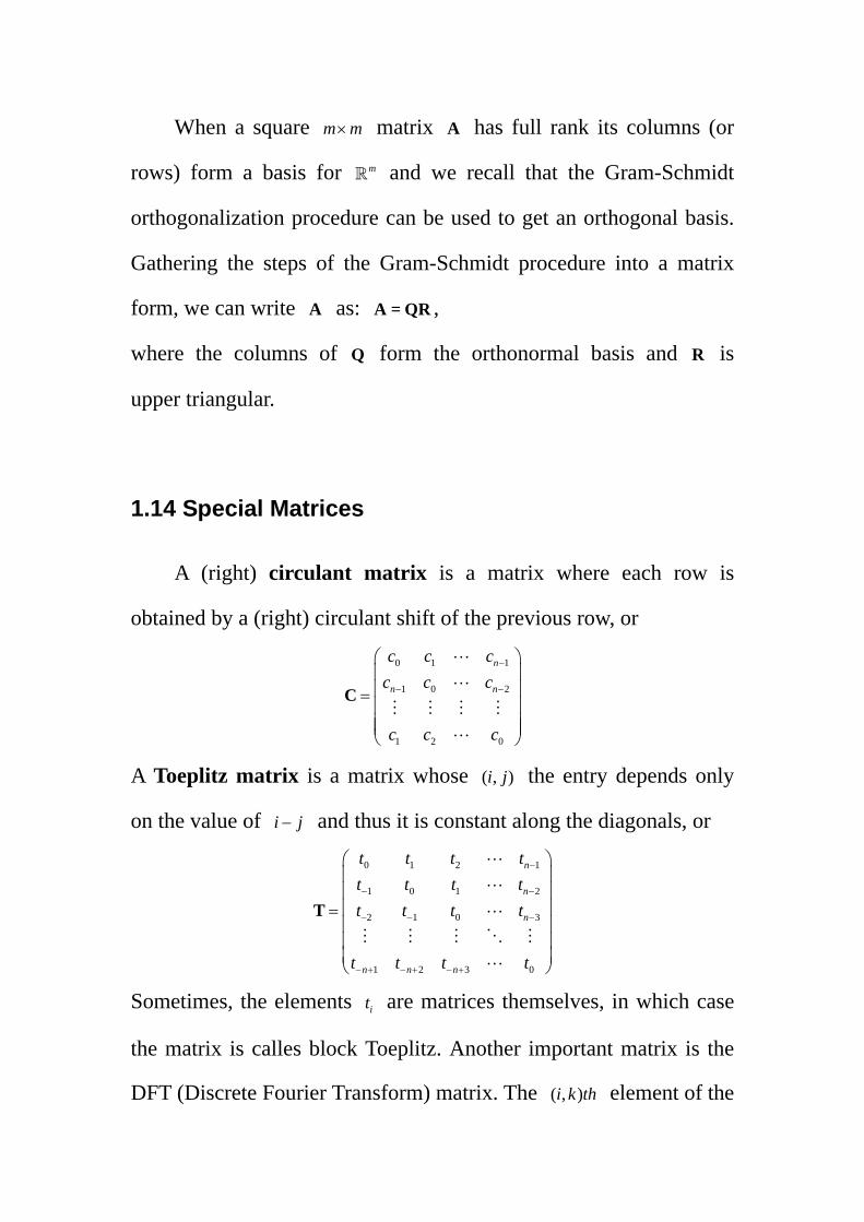
A (right) circulant matrix is a matrix where each row is

obtained by a (right) circulant shift of the previous row, or

0 1 1

1 0 2

1 2 0

n

n n

c c cc c c

c c c

−

− −

⎛ ⎞⎜ ⎟⎜ ⎟=⎜ ⎟⎜ ⎟⎜ ⎟⎝ ⎠

C

A Toeplitz matrix is a matrix whose ( , )i j the entry depends only

on the value of i j− and thus it is constant along the diagonals, or

0 1 2 1

1 0 1 2

2 1 0 3

1 2 3 0

n

n

n

n n n

t t t tt t t tt t t t

t t t t

−

− −

− − −

− + − + − +

⎛ ⎞⎜ ⎟⎜ ⎟⎜ ⎟=⎜ ⎟⎜ ⎟⎜ ⎟⎝ ⎠

T

Sometimes, the elements it are matrices themselves, in which case

the matrix is calles block Toeplitz. Another important matrix is the

DFT (Discrete Fourier Transform) matrix. The ( , )i k th element of the

DFT matrix of size n n× is 2 /ik i ik nnW e π−= . The DFT matrix

diagonalizes circulant matrices, that is, its columns and rows are the

eigenvectors of circulant matrices.

A real symmetric matrix A is called positive definite if all its

eigenvalues are greater than 0. Equivalently, for all nonzero vectors

x , the following is satisfied: 0T >Ax x .

Finally, for a positive definite matrix A , there exists a nonsingular

matrix W such that: T=A W W ,

where W is intuitively a “square root” of A . One possible way to

choose such a square root is to diagnolize A as

TA = Q QΛ

and then, since all the eigenvalues are positive, choose TW = Q Λ

(the square root is applied on each eigenvalue in the diagonal matrix

Λ ).

A polynomial matrix (or a matrix polynomial) is a matrix

whose entries are polynomials. The fact that the above two names

can be used interchangeably is due to the following forms of a

polynomial matrix ( )

i ii i

ii

ii ii i

a x b xx x

c x d x

⎛ ⎞⎜ ⎟

= =⎜ ⎟⎜ ⎟⎝ ⎠

∑ ∑∑

∑ ∑H H

that is, it can be written either as a matrix containing polynomials as

its entries, or a polynomial having matrices as its coefficients.

The question of the rank in polynomial matrices is more subtle.

For example, the matrix:

3( )( )

a bx a bxc dx c dxλ+ +⎛ ⎞

⎜ ⎟+ +⎝ ⎠

for 3,λ = the normal rank is 1, while for 2λ = , the normal rank is 2.

An important class of polynomial matrices are unimodular

matrices, whose determinant is not a function of x. An example is the

following matrix:

1( )

2 1x x

xx x

+⎛ ⎞= ⎜ ⎟+ +⎝ ⎠

H

whose determinant is equal to 1. There are several useful properties

pertaining to unimodular matrices. For example, the product of two

unimodular matrices is again unimodular. The inverse of a

unimodular matrix is unimodular as well. Also, one can prove that a

polynomial matrix ( )xH is unimodular, if and only if its inverse is a

polynomial matrix. (See also the properties of determinants)

The extension of the concept of unitary matrices to polynomial

matrices leads to paraunitary matrices as studied in circuit theory. In

fact, these matrices are unitary on the unit circle or the imaginary

axis, depending if they correspond to discrete-time or

continuous-time linear operators ( z -transforms or Laplace

transforms). Consider the discrete-time case and ix e ω= . Then, a

square matrix ( )xU is unitary on the unit circle if: * *

( ) ( ) ( ) ( )i i i ie e e eω ω ω ω⎡ ⎤ ⎡ ⎤= =⎣ ⎦ ⎣ ⎦U U U U I

Extending this beyond the unit circle leads to 1 1( ) ( ) ( ) ( )

T Tx x x x− −⎡ ⎤ ⎡ ⎤= =⎣ ⎦ ⎣ ⎦U U U U I

If the coefficients of the polynomials are complex, the coefficients

need to be conjugated, which is usually written 1( )T

x−⎡ ⎤⎣ ⎦*U .

As a generalization of polynomial matrices, one can consider

the case of rational matrices, where each entry is a ratio of two

polynomials. Unimodular and unitary matrices can be defined in the

rational case, as in the polynomial case.

1.15 Fourier Transform

Fourier Transform in ( )1L :

The Fourier integral

ˆ ( ) ( ) , ( )i t i tf f t e dt e f tω ωω+∞ −

−∞= =∫

measures “how much” oscillators at the frequency ω there is in f.

Theorem: If ( )f ∈ 1L and ˆ ( )f ∈ 1L then

1 ˆ( ) ( )2

i tf t f e dωω ωπ

+∞

−∞= ∫ .

Note:

(1) Note that i te ω is not in ( )2L , and that the set i te ω is not

countable.

(2) The inverse formula decomposes f as a sum of sinusoidal

waves i te ω of amplitude ˆ ( )f ω . The hypothesis ˆ ( )f ∈ 1L implies

that f must be continuous ( ˆ ( ) ( )f f t dtω+∞

−∞≤ < +∞∫ ), so the

reconstruction is not proved for discontinuous functions. For

example, the inversion is exact if ( )f t is continuous ( or if ( )f t is

defined as ( ( ) ( )) / 2f t f t+ −+ at a point of discontinuity.

Theorem (Convolution): Let ( )f ∈ 1L and ( )h∈ 1L . The

function g f h= ∗ is in ( )1L and ˆˆ ( ) ( ) ( )g f hω ω ω=

Important properties of Fourier transform:

Property Function Fourier Transform

( )f t ˆ ( )f ω

Inverse ˆ ( )f t 2 ( )fπ ω−

Convolution 1 2 ( )f f t∗ 1 2( ) ( )f fω ω

Multiplication 1 2( ) ( )f t f t 1 21 ˆ( ) ( )

2f fω ω

π∗

Translation ( )f t u− ˆ ( )iue fω ω−

注：一信号在时域中延迟一时间 u，则在频域中所有的信号频

谱分量，都将给予一个对频率成线性关系的滞后相移 uω 。

Modulation ( )i te f tξ ˆ ( )f ω ξ−

注：一个信号在时域中与因子 i te ζ 相乘，等效于在频域中将整

个频谱向频率增加方向搬移ζ ；实用中，是把时间函数与正弦函

数相乘（与频率为ζ 的正弦函数相乘），等效于在频域中将频谱

同时向频率正负方向搬移ζ ，等同于数字通信中的调幅。

Scaling ( )tfs

ˆ ( )s f sω

注：对于一定信号，脉冲宽度与频带宽度间存在反比关系，

二者乘积为一常数。实际应用中，希望选择一脉冲，其脉宽与频

宽乘积是一个尽可能小的常数，以便两者都可取较小数值，如高

斯脉冲。

Time derivatives ( ) ( )pf t ˆ( ) ( )pi fω ω

Time integral ( ) ( )pf t− ˆ( ) ( )pi fω ω−

注：信号在时域中的求导，相当于在频域中用因子 iω去乘它

的频谱函数。

Frequency derivatives ( ) ( )pit f t− ( )ˆ ( )pf ω

Complex conjugate *( )f t *ˆ ( )f ω−

Hermitian symmetry ( )f t ∈ *ˆ( ) ( )f fω ω− =

Momens:

Calling ( ) , 0,1, 2,nnm t f t dt n

∞

−∞= =∫ ,

the moment theorem of the Fourier transform states that

0

ˆ ( )( ) | , 0,1, 2,n

nn n

fi m nωδ ωδω =− = =

Convolution:

( ) ( ) ( )h t f g t dτ τ τ∞

−∞= −∫

ˆ( ) ( ) ( ) ( )f t g t f gω ω∗ ↔ 1 ˆ( ) ( ) ( ) ( )

2f t g t f gω ω

π↔ ∗

Commutativity: ( ) ( )f h t h f t∗ = ∗

Differentiation: ( )( ) ( ) ( )d df dhf h t h t f tdt dt dt

∗ = ∗ = ∗

Dirac convolution: ( ) ( )f t f tτδ τ∗ = −

( )( )

( )

' [ ( ) ( )] ˆ( ) ( ) ( )

ˆ ( ) ( )

ˆ ( ) ( )

f t g th t i f gt

i f g

f i g

δ ω ω ωδ

ω ω ω

ω ω ω

∗= ↔

=

=

, ' ( ) ( ) ( ) ( ) ( )h t f t g t f t g t′ ′= ∗ = ∗

This is useful when convolving a signal with a filter which is

known to be the derivative of a given function such as a Gaussian,

since one can think of the result as being the convolution of the

derivative of the signal with a Gaussian.

Parseval’s Formula

Because the Fourier transform is an orthogonal transform, it

satisfies an energy conservation relation known as Parseval’s

formula. * *1 ˆ ˆ( ) ( ) ( ) ( )

2f t g t dt f g dω ω ω

π∞ ∞

−∞ −∞=∫ ∫

when ( ) ( )g t f t= , 22 1 ˆ( ) ( )

2f t dt f dω ω

π∞ ∞

−∞ −∞=∫ ∫

Note that the factor 1/ 2π comes from our definition of the

Fourier transform. A symmetric definition, with a factor 1/ 2π in

both the analysis and synthesis formulas, would remove the scale

factor.

注 1：单边频谱与希尔伯特变换

一个时间实函数信号 ( )f t 的频谱函数是一个复数频谱，因振幅

频谱或频谱函数的实部对ω为偶对称，相位频谱或频谱函数的虚

部对ω为奇对称：因此

（1）如 ( )f t 为 t的偶函数，则其频谱函数仅有实部（为ω的实

偶函数）；如 ( )f t 为 t的奇函数，则其频谱函数仅有虚部（为ω的

虚奇函数）

（2）正谱与负谱互成共轭复数关系： *ˆ ( ) ( )f fω ω= −

即正谱一旦确定，则负谱亦随之确定。因而如去除负谱部分

构成单边频谱，信号包含的信息并不会丢失，只是单边频谱对应

的时间信号不是一个时间的实函数信号，而是一个时间的复函数

信号，称为解析信号。

单边频谱，可以将双边频谱的负谱部分对称于纵轴反褶后加

到正谱上来获得，即：

ˆ2 ( ) 0ˆ ( ) ( )[1 sgn( )]0 0s

ff f ω ωω ω ωω

⎧ >⎪= + = ⎨<⎪⎩

1 1 ( )( ) ( ) [ ( ) ] ( )

( ) ( )

sff t f t t i f t i d

t tf t if t

τδ τπ π τ

∞

−∞= ∗ + = +

−= +

∫ ，

1sgn( ) it

ωπ

↔∵ ，1 ( )( ) ff t d

tτ τ

π τ∞

−∞=

−∫

可见，双边谱的时间信号 ( )f t ，即为单边频谱解析信号的实部，

解析信号的虚部 ( )f t 即为实部 ( )f t 的希尔伯特变换。

且： ˆ ˆ( ) ( )sgn( )f ifω ω ω= − ， ˆ( ) ( ) ( )sgn( ) sgn( )f t f if iω ω ω ω↔ = − ⋅∵

1 1 ( )( ) ( ) ff t f t dt t

τ τπ π τ

∞

−∞∴ = ∗− = −

−∫

希尔伯特正、反变换仅差一负号。

注 2：常用函数及其傅里叶频谱：

（1）矩形脉冲频谱（门函数 ( ), ( , )2 2

G tττ τ

− ，A为脉冲幅度）： 2ˆ( ) ( ) ( ) ( ) sin ( )

2 2 2 2AG t u t u t f A Saτ

τ τ ωτ ωτω τω

= + − − ↔ = =

（2）抽样函数 sin / 2 2( ) ( ) ( ) ( )2 / 2 2 2t tSa G u u

tπω ω ωΩ

Ω Ω Ω Ω⎡ ⎤= ↔ = + − −⎢ ⎥Ω Ω ⎣ ⎦

（3）单边指数信号 1( )ate u ta iω

− ↔+

双边指数信号 2 2

2a t aea ω

− ↔+

指数脉冲： 2

1( )( )

atte u ta iω

− ↔+

（4）单位冲激： ( ) 1tδ ↔ ，

单位阶跃： 21( ) ( )i

u t eπ

πδ ωω

−↔ + ，

单位直流：1 2 ( )πδ ω↔

符号函数：2sgn( )t

iω↔

（5）指数函数： 2 ( )ci tce ω πδ ω ω↔ − ，

单位余弦： cos [ ( ) ( )]c c ctω π δ ω ω δ ω ω↔ + + −

单位正弦： sin [ ( ) ( )]c c ct iω π δ ω ω δ ω ω↔ + − −

阶跃正弦： 2 2sin ( ) [ ( ) ( )]2

cc c c

c

tu ti

ωπω δ ω ω δ ω ωω ω

↔ − − + +−

阶跃余弦： 2 2cos ( ) [ ( ) ( )]2c c c

c

itu t π ωω δ ω ω δ ω ωω ω

↔ − + + +−

减幅正弦： 2 2sin ( )( )

at cc

c

e tu ta i

ωωω ω

− ↔+ +

升余弦脉冲：2

2 2 2

2 8 sin( / 2)1 cos ( ) ( )2 2 (4 )T T Tt u t u t

T Tπ π ω

ω π ω⎛ ⎞ ⎡ ⎤+ + − − ↔⎜ ⎟ ⎢ ⎥ −⎝ ⎠ ⎣ ⎦

半余弦脉冲： 2 2 2

2 cos( / 2)cos ( ) ( )2 2 1 /

t u t u tπ τ τ τ τωτ π τ ω π

⎡ ⎤+ − − ↔⎢ ⎥ −⎣ ⎦

（6）三角形脉冲：

2 2| |1 | | sin( / 2)ˆ( ) ( )

2 / 20 | |

t tf t f Sa

t

τ ωτ ωτω τ ττωττ

⎧ − < ⎡ ⎤⎪ ⎛ ⎞ ⎡ ⎤= ↔ = =⎨ ⎜ ⎟⎢ ⎥ ⎢ ⎥⎝ ⎠ ⎣ ⎦⎣ ⎦⎪ >⎩

高斯脉冲：22

2t

e eτω

τ πτ⎛ ⎞−− ⎜ ⎟⎝ ⎠↔

冲激序列： ( ) ( )Tn

t t nTδ δ∞

=−∞

= −∑

1ˆ ( ) ( ) ( )2

2 ( ) ( )

in tn n

n n

n

f Lf t L A e A n

nT

ω π δ ω

π δ ω δ ω

∞ ∞Ω

=−∞ =−∞

∞

Ω=−∞

⎧ ⎫↔ = = = − Ω⎨ ⎬

⎩ ⎭

= − Ω = Ω

∑ ∑

∑

Fourier Transform in ( )2L :

Considering the Fourier transform of the indicator function

[ 1,1]f −= 1 is 1

1

2sinˆ ( ) i tf e dtω ωωω

−

−= =∫ . This function is not integrable

because f is not continuous, but its square is integrable. This

motivates the extension of the Fourier transform to the space ( )2L

of functions f with a finite energy 2( )f t dt+∞

−∞< +∞∫ .

By working in the Hilbert space ( )2L , we also have access to

all the facilities provided by the existence of an inner product.

Theorem (Parseval and Plancherel formulas): If f and h are in

( ) ( )1 2L L∩ then * *1 ˆ( ) ( ) ( ) ( )2

f t h t dt f h dω ω ωπ

+∞ +∞

−∞ −∞=∫ ∫ . For h f=

it follows that 22 1 ˆ( ) ( )

2f t dt f dω ω

π+∞ +∞

−∞ −∞=∫ ∫ .

Proof: Let *( )g f h t= ∗ − , then *ˆˆ ( ) ( ) ( )g f hω ω ω= , therefore

* *1 1 ˆˆ( ) ( ) (0) ( ) ( ) ( )2 2

f t h t dt g g d f h dω ω ω ω ωπ π

+∞ +∞ +∞

−∞ −∞ −∞= = =∫ ∫ ∫

Density Extension in ( )2L :

If ( )f ∈ 2L but ( )f ∉ 1L , its Fourier transform cannot be

calculated with the Fourier integral because ( ) i tf t e ω− is not

integrable.

Since ( ) ( )1 2L L∩ is dense in ( )2L , one can find a family

n nf

∈ of functions in ( ) ( )1 2L L∩ that converges to f:

lim 0nnf f

→∞− = . Since n n

f∈

converges, it is a Cauchy sequence,

which means that n pf f ε− < if n and p are larger enough.

Moreover, ( )nf ∈ 1L so its Fourier transform nf is well defined.

The Plancherel formula proves that n nf

∈ is also a Cauchy

sequence because ˆ 2n p n pf f f fπ− = − is arbitrarily small for n

and p larger enough.

Owing to the completeness, all Cauchy sequences converge to an

element of the space. Hence, there exists ˆ ( )f ∈ 2L such that

ˆlim 0nnf f

→∞− = .

Therefore, the extension of the Fourier transform to ( )2L

satisfies the convolution theorem, the Parseval and Plancherel

formulas as well as properties.

Diracs:

Since 1i te ω = at 0t = it seems reasonable to define its Fourier

transform by ˆ( ) ( ) 1i tt e dtωδ ω δ+∞ −

−∞= =∫

Examples:

The indicator function [ , ]T Tf −= 1 is discontinuous at

t T= ± . 2sin( )ˆ ( )T i t

T

Tf e dtω ωωω

−

−= =∫

An ideal low-pass filter has a transfer function [ , ]h ξ ξ−= 1

that selects low frequencies over [ , ]ξ ξ− ,

1 sin( )( )2

i t th t e dt

ξ ω

ξ

ξωπ π−

= =∫ .

A passive electronic circuit implements analog filters with

resistances, capacities and inductors. The input voltage f(t)

is related to the output voltage g(t) by a differential

equation with constant coefficients:

( ) ( )

0 0

( ) ( )K M

k kk k

k k

a f t b g t= =

=∑ ∑ .

Suppose that the circuit is not charged for 0t < , which

means that ( ) ( ) 0f t g t= = . The output g is a linear

time-invariant function of f and can thus be written g f h= ∗ ,

and 0

0

( )ˆ ( )ˆ( ) ˆ ( ) ( )

Kk

kkM

kk

k

a ighf b i

ωωωω ω

=

=

= =∑

∑. It is a rational function of iω .

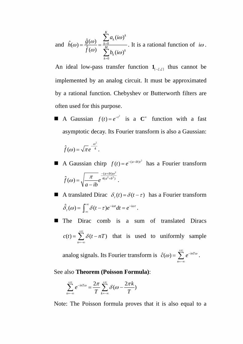
An ideal low-pass transfer function [ , ]ξ ξ−1 thus cannot be

implemented by an analog circuit. It must be approximated

by a rational function. Chebyshev or Butterworth filters are

often used for this purpose.

A Gaussian 2

( ) tf t e−= is a ∞C function with a fast

asymptotic decay. Its Fourier transform is also a Gaussian: 2

4ˆ ( )f eω

ω π−

= .

A Gaussian chirp 2( )( ) a ib tf t e− −= has a Fourier transform 2

2 2( )

4( )ˆ ( )a iba bf e

a ib

ωπω

− ++=

−.

A translated Dirac ( ) ( )t tτδ δ τ= − has a Fourier transform

ˆ ( ) ( ) i t it e dt eω ωττδ ω δ τ

+∞ − −

−∞= − =∫ .

The Dirac comb is a sum of translated Diracs

( ) ( )n

c t t nTδ+∞

=−∞

= −∑ that is used to uniformly sample

analog signals. Its Fourier transform is ˆ( ) inT

n

c e ωω+∞

−

=−∞

= ∑ .

See also Theorem (Poisson Formula):

2 2( )inT

n k

keT T

ω π πδ ω+∞ +∞

−

=−∞ =−∞

= −∑ ∑

Note: The Poisson formula proves that it is also equal to a

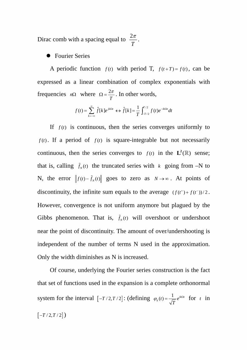
Dirac comb with a spacing equal to 2Tπ .

Fourier Series

A periodic function ( )f t with period T, ( ) ( )f t T f t+ = , can be

expressed as a linear combination of complex exponentials with

frequencies nΩ where 2Tπ

Ω = . In other words,

ˆ( ) [ ] jk t

k

f t f k e∞

Ω

=−∞

= ∑/ 2

/ 2

1ˆ[ ] ( )T ik t

Tf k f t e dt

T− Ω

−↔ = ∫

If ( )f t is continuous, then the series converges uniformly to

( )f t . If a period of ( )f t is square-integrable but not necessarily

continuous, then the series converges to ( )f t in the ( )2L sense;

that is, calling ( )Nf t the truncated series with k going from –N to

N, the error ( ) ( )Nf t f t− goes to zero as N →∞ . At points of

discontinuity, the infinite sum equals to the average ( ( ) ( )) / 2f t f t+ −+ .

However, convergence is not uniform anymore but plagued by the

Gibbs phenomenon. That is, ( )Nf t will overshoot or undershoot

near the point of discontinuity. The amount of over/undershooting is

independent of the number of terms N used in the approximation.

Only the width diminishes as N is increased.

Of course, underlying the Fourier series construction is the fact

that set of functions used in the expansion is a complete orthonormal

system for the interval [ ]/ 2, / 2T T− : (defining 1( ) ik tk t e

Tϕ Ω= for t in

[ ]/ 2, / 2T T− )

2/ 2 ( )

/ 2

1 1( ), ( ) sin( ( ))( )

T i l k tT

k l Tt t e dt l k

T l k

π

ϕ ϕ ππ

−

−= = −

−∫

Parseval’s Relation

With the Fourier series coefficients are defined and the inner

product of periodic functions taken over one period, we have

[ , ]2 2

ˆ ˆ( ), ( ) [ ], [ ]T Tf t g t T f k g k−

=

where the factor T is due to the normalization chosen. In particular,

for ( ) ( )g t f t= , 2

[ , ]2 2

ˆ( ) [ ]T Tf t T f k−

=

1.16 Properties

Stability and Causality:

A filter is said to be causal if ( )Lf t does not depend on the

values ( )f u for u t> . Since ( ) ( ) ( )Lf t h u f t u du+∞

−∞= −∫ , this means

that ( ) 0h u = for 0u < .

The stability property guarantees that ( )Lf t is bounded if ( )f t

is bounded. Since ( ) ( ) ( ) sup ( ) ( )u

Lf t h u f t u du f u h u du+∞ +∞

−∞ −∞∈≤ − ≤∫ ∫ ,

it is sufficient and necessary condition that ( )h t dt+∞

−∞< +∞∫ . We thus

say that h is stable if it is integrable.

Example:

A uniform averaging of f over intergrals of size T is calculated by

2

2

1( ) ( )t T

t TLf t f u du

T+

−= ∫ , this integral can be rewritten as a

convolution of f with the impulse response [ 2, 2]1

T ThT −= 1 .

注：相关与卷积

( ) ( ) ( ) ( ) ( ) ( ) ( )xyR t x y t d x t y d x t y tτ τ τ τ τ τ∞ ∞

−∞ −∞= − = + = ∗ −∫ ∫

( ) ( )xy yxR t R t= −

( ) ( )xx xxR t R t= −

即某一 t 时刻的相关系数 ( )xyR t ，表示信号 ( )x τ 与另一延时 t

时间的信号相乘后所得曲线下的面积；与卷积的图解区别仅在于

延时前 ( )y τ 不经过反褶而已。

Regularity and Decay:

The global regularity of a signal f depends on the decay of ˆ ( )f ω

when the frequency ω increases. If ˆ ( )f ∈ 1L , then the Fourier

inversion formula implies that f is continuous and bounded:

1 1 ˆ( ) ( ) ( )2 2

i tf t e f d f dω ω ω ω ωπ π

+∞ +∞

−∞ −∞≤ = < +∞∫ ∫ .

Proposition: A function f is bounded and p times continuously

differentiable with bounded derivatives if ˆ ( ) (1 )pf dω ω ω+∞

−∞+ < +∞∫ .

Proof: ( ) ( )kf t ˆ( ) ( )ki fω ω⇔

Note: This is a sufficient condition that guarantees the

differentiability of f at any order p.

This result proves that if there exist a constant K and

0ε > such that 1ˆ ( )

1 pKf εωω + +≤

+, then pf ∈C . If f has a

compact support then it implies that f ∞∈C .

The decay of ˆ ( )f ω depends on the worst singular behavior of f.

For example, [ , ]T Tf −= 1 is discontinuous at t T= ± , so ˆ ( )f ω

decays like 1ω − . In this case, it could also be important to know that

( )f t is regular (光滑) for t T≠ ± . This information cannot be

derived from the decay of ˆ ( )f ω . To characterize local regularity of

a signal f it is necessary to decompose it over waveforms that are

well localized in time, as opposed to sinusoidal waves i te ω .

Uncertainty Principle:

Can we construct a function f whose energy is well localized in

time and whose Fourier transform f has an energy concentrated in

a small frequency neighborhood?

The Dirac ( )t uδ − has a support restricted to t u= but its

Fourier transform i ue ω− has an energy uniformly spread over all

frequencies. ˆ ( )f ω decays quickly at high frequencies only if f has

regular variations in time. Therefore, the energy of f must be spread

over a relatively large domain.

To reduce the time spread of f, we can scale it by 1s < while

maintaining constant its total energy. If 1( ) ( )stf t fss

= then

2 2sf f= . The Fourier transform ˆ ( ) ( )sf s f sω ω= is dilated by 1

s

so we lose in frequency localization what we gained in time.

Underlying is a trade-off between time and frequency localization.

Time and frequency energy concentrations are restricted by the

Heisenberg uncertainty principle. This principle has a particularly

important interpretation in quantum mechanics as an uncertainty as

to the position and momentum of a free particle. The state of a

one-dimensional particle is described by a wave function ( )f ∈ 2L .

The probability density that this particle is located at t is 22

1 ( )f tf

.

The probability density that its momentum is equal to ω is 2

21 ˆ ( )

2f

fω

π.

The average location of this particle is 22

1 ( )u t f t dtf

+∞

−∞= ∫ ,

The average momentum is 2

21 ˆ ( )

2f d

fξ ω ω ω

π

+∞

−∞= ∫ ,

The variances around these average values are respectively

22 22

1 ( ) ( )t t u f t dtf

σ+∞

−∞= −∫ and

22 2

21 ˆ( ) ( )

2f d

fωσ ω ξ ω ωπ

+∞

−∞= −∫ .

The larger tσ , the more uncertainty there is concerning the position

of the free particle; the larger ωσ , the more uncertainty there is

concerning its momentum.

Theorem (Heisenberg Uncertainty): The temporal variance and

the frequency variance of ( )f ∈ 2L satisfy 2 2 14t ωσ σ ≥ . This

inequality is an equality if and only if there exist 2 2( , , , )u a bξ ∈ ×

such that 2( )( ) i t b t uf t ae ξ − −= .

Proof:

Suppose that lim ( ) 0t

t f t→+∞

= . If the average time and frequency

localization of f is u and ξ , then the average time and frequency

location of ( )i te f t uξ− + is zero. It is thus sufficient to prove the

theorem for 0u ξ= = . Observe that 222 2

41 ˆ( ) ( )

2t tf t dt f dfωσ σ ω ω ω

π

+∞ +∞

−∞ −∞= ∫ ∫ .

Since ' ˆ( ) ( )f t i fω ω⇔ , 222 2 '

41 ( ) ( )t tf t dt f t dtfωσ σ

+∞ +∞

−∞ −∞= ∫ ∫

Schwarz’s inequality implies:

( )

22 2 ' *

4

2' * '*

4

2'24

1 ( ) ( )

1 [ ( ) ( ) ( ) ( )]2

1 1 ( )44

t tf t f t dtf

t f t f t f t f t dtf

t f t dtf

ωσ σ+∞

−∞

+∞

−∞

+∞

−∞

⎡ ⎤≥ ⎢ ⎥⎣ ⎦

⎡ ⎤≥ +⎢ ⎥⎣ ⎦

⎡ ⎤≥ =⎢ ⎥⎣ ⎦

∫

∫

∫

To obtain an equality, Schwarz’s inequality must be an equality.

This implies that there exists b∈ such that ' ( ) 2 ( )f t btf t= − .

Hence, there exists a∈ such that 2

( ) btf t ae−= . When 0u ≠ and

0ξ ≠ the corresponding time and frequency translations are

2( )( ) i t b t uf t ae ξ − −= .

Compact Support (紧支集):

Despite the Heisenberg uncertainty bound, we might still enable

to construct a function of compact support whose Fourier transform

has a compact support. Such a function would be very useful in

constructing a finite impulse response filter with a band-limited

transfer function. Unfortunately, the following theorem proves that it

does not exist （在时、频域均是紧支集的函数是不存在的）.

Theorem: If 0f ≠ has a compact support then ˆ ( )f ω cannot be

zero on a whole interval (Compact support). Similarly, if ˆ 0f ≠ has

a compact support then ( )f t cannot be zero on a whole interval

(Compact support).

Proof: (反证法)

If f has a compact support included in [ , ]b b− then

1 ˆ( ) ( )2

b i t

bf t f e dωω ω

π+

−= ∫ .

If ( ) 0f t = for [ , ]t c d∈ , by differentiating n times under the

integral at 0 2c dt +

= ( 两 边 n 次 微 分 ), we obtain

0( )0

1 ˆ( ) ( )( ) 02

b i tn n

bf t f i e dωω ω ω

π −= =∫ .

Since 0 0( )1 ˆ( ) ( )2

b i t t i t

bf t f e e dω ωω ω

π−

−= ∫ , developing 0( )i t te ω − as an

infinite series yields for all t∈ ,

00

0

1 [ ( )] ˆ( ) ( ) 02 !

n b i tn

bn

i t tf t f e dn

ωω ω ωπ

+∞

−=

−= =∑ ∫ , which contradicts our

assumption that 0f ≠ .

Total Variation:

The total variation measures the total amplitude of signal

oscillations. Its value depends on the length of the image level sets

for image processing. We show that a low-pass filter can

considerably amplify the total variation by creating Gibbs

oscillations.

Variation and Oscillations: If f is differentiable, its total

variation is defined by '( )V

f f t dt+∞

−∞= ∫ . If p p

x are the abscissa

(横坐标，集合) of the local extreme of f where '( ) 0pf x = , then

1( ) ( )p pVp

f f x f x+= −∑ .

It measures the total amplitude of the oscillations of f. For

example, if 2

( ) tf t e−= , then 2V

f = . If sin( )( ) tf ttπ

π= , then f has a

local extrema at [ , 1]px p p∈ + for any p∈ . Since 1

1( ) ( )p pf x f x p −+ − ∼ , we derive that

Vf = +∞ .

The total variation of non-differentiable functions can be

calculated by considering the derivative in the general sense of

distributions: ( ) ( )lim

V x

f t f t hf dt

h+∞

−∞→∞

− −= ∫ . For example, if

[ , ]a bf = 1 then 2V

f = . We say that f has a bounded variation if

Vf < +∞ .

Because of 'ˆ ( ) ( )f i fω ω ω= , 'ˆ ( ) ( )V

f f t dt fω ω+∞

−∞≤ =∫ and

ˆ ( ) Vf

f ωω

≤ . However, 1ˆ ( ) ( )f Oω ω −= is not a sufficient

condition to guarantee that f has a bounded variation. For example, if

sin( )( ) tf ttπ

π= then [ , ]f π π−= 1 satisfied 1ˆ ( )f ω π ω −≤ although

Vf = +∞ . In general, the total variation of f cannot be evaluated

from ˆ ( )f ω

Discrete Signals

Let [ ] ( )Nnf n fN

= be a discrete signal obtained with a uniform

sampling at interval 1N − , [ ] [ 1]N N NVn

f f n f n= − −∑ . If pn are the

abscissa (横坐标，集合 ) of the local extreme of fN, then

1[ ] [ ]N N p N pVp

f f n f n+= −∑ .

The discrete signal has a bounded variation if N Vf is bounded

by a constant independent of the resolution N.

Gibbs Oscillations:

Filtering a signal with a low-pass filter can create oscillations

that have an infinite total variation. Let f f hξ ξ= ∗ be the filtered

signal obtained with an ideal low-pass filter whose transfer function

is [ , ]hξ ξ ξ−= 1 . If ( )f ∈ 2L , then fξ converges to f in ( )2L norm:

lim 0f fξξ→+∞− = . Indeed, [ , ]f fξ ξ ξ−= 1 implies that

222 1 1 ˆ( ) ( ) ( )2 2

f f f f d f dξ ξ ω ξω ω ω ω ω

π π+∞

−∞ >− = − =∫ ∫ , which goes

to zero as ξ increases. However, if f is discontinuous in 0t , then we

show that fξ has Gibbs oscillations in the neighborhood of 0t ,

which prevents sup ( ) ( )t

f t f tξ∈

− from converging to zero as ξ

increases.

Let f be a bounded variation function V

f < +∞ that has an

isolated discontinuity at 0t , with a left limit 0( )f t− and right limit

0( )f t+ . It is decomposed as a sum of cf , which is continuous in the

neighborhood of 0t , plus a Heaviside step of amplitude

0 0( ) ( )f t f t+ −− :

0 0 0( ) [ ( ) ( )] ( )cf t f f t f t u t t+ −= + − − with 1 0

( )0

if tu t

otherwise≥⎧

= ⎨⎩

Hence 0 0 0( ) ( ) [ ( ) ( )] ( )cf t f h t f t f t u h t tξ ξ ξ+ −= ∗ + − ∗ − .

We can prove that ( )cf h tξ∗ converges uniformly to ( )cf t in a

neighborhood of 0t . The following proposition shows that this is not

true for u hξ∗ , which creates Gibbs oscillations.

Preposition (Gibbs): For any 0ξ > , sin( )t xu h t dx

xξ

ξ π−∞∗ = ∫ .

The function sin( )t xs t dx

xξ

ξπ−∞

= ∫ is a sigmoid that increases from

zero at t = −∞ to 1 at t = +∞ , with 1(0)2

s = . It has oscillations of

period πξ

, which are attenuated when the distance to 0 increases,

but their total variation is infinite: V

s = +∞ . The maximum

amplitude of the Gibbs oscillations occurs at t πξ

= , with an

amplitude independent of ξ : sin( ) 1 1 0.045xA s dxx

ππ

π−∞= − = − ≈∫ .

0 0 0( ) ( ) [ ( ) ( )] ( ( )) ( , )f t f t f t f t s t t tξ ξ ε ξ+ −− = − − +

where 0

lim sup ( , ) 0t t

tξ α

ε ξ→+∞ − <

= in some neighborhood of size 0α >

around 0t . The sigmoid 0( ( ))s t tξ − centered at 0t creates a

maximum error of fixed amplitude for all ξ . The Gibbs oscillations

have an amplitude proportional to the jump 0 0( ) ( )f t f t+ −− at all

frequencies ξ .

Image Total Variation:

The total variation of an image 1 2( , )f x x depends on the

amplitude of its variations as well as the length of the contours along

which they occur. Suppose that 1 2( , )f x x is differentiable. The total

variation is defined by: 1 2 1 2( , )V

f f x x dx dx= ∇∫ ∫ , where the

modulus of the gradient vector is:

12 2 2

1 2 1 21 2

1 2

( , ) ( , )( , ) f x x f x xf x xx x

⎛ ⎞∂ ∂⎜ ⎟∇ = +⎜ ⎟∂ ∂⎝ ⎠

As in one dimension, the total variation is extended to

discontinuous functions by taking the derivatives in the general

sense of distributions. An equivalent norm is obtained by

approximating the partial derivatives by finite differences:

12 2 2

1 2 1 2 1 2 1 21 2

( , ) ( , ) ( , ) ( , )( , )hf x x f x h x f x x f x x hf x x

h h⎛ ⎞− − − −

∆ = +⎜ ⎟⎜ ⎟⎝ ⎠

One can verify that:

1 2 1 20lim ( , ) 2hV Vh

f f x x dx dx f→

≤ ∆ ≤∫ ∫

The finite difference integral gives a large value when 1 2( , )f x x is

discontinuous along a diagonal line in the 1 2( , )x x plane.

The total variation of f is related to the length of its level sets. Let

us define 21 2 1 2( , ) : ( , )y x x f x x yΩ = ∈ > . If f is continuous then the

boundary y∂Ω of yΩ is the level set of all 1 2( , )x x such that

1 2( , )f x x y= . Let 1( )yH ∂Ω be the length of y∂Ω . Formally, this

length is calculated in the sense of the monodimensional Hausdorff

measure. The following theorem relates the total variation of f to the

length of its level sets.

Theorem (Co-Area Formula): If V

f < +∞ then

1( )yVf H dy

+∞

−∞= ∂Ω∫ .

Proof:

See also: M. Antonini, M. Barlaud, P. Mathieu, and I. Daubechies,

Image coding using wavelet transform. IEEE Trans. Image

Processing, 1(2): 205-220, Apr. 1992.

Give an intuitive explanation when f is continuously differentiable.

In this case y∂Ω is a differentiable curve 2( , )x y s ∈ , which is a

parameterized by the arc-length s. Let ( )xτ be the vector tangent

(切向量 ) to this curve in the plane. The gradient ( )f x∇ is

orthogonal to ( )xτ . The Frenet coordinate system along y∂Ω is

composed of ( )xτ and of the unit vector ( )n x parallel to ( )f x∇ .

Let ds and dn be the lebesgue measures in the direction of ( )xτ and

( )n x . We have: ( ) ( ) dyf x f x ndn

∇ =∇ ⋅ = ,

where dy is the differential of amplitudes arcoss level sets. The idea

of the proof is to decompose the total variation integral over the

planes as an integral along the level sets and across level sets, which

we write: 1 2 1 2 1 2

1

( ) ( )

( )

y

y

V

y

f f x x dx dx f x x dsdn

dsdy H dy

∂Ω

+∞

∂Ω −∞

= ∇ = ∇

= = ∂Ω

∫ ∫ ∫ ∫

∫ ∫ ∫, where

1( )y

yds H∂Ω

= ∂Ω∫ is the length of the level set.

The Co-area formula gives an important geometrical

interpretation of the total image variation. Images are uniformly

bounded so the integral is calculated over a finite interval and is

proportional to the average length of level sets. It is finite as long as

the level sets are not fractal curves. In general, bounded variation

images must have a step edges of finite length.

Discrete Images:

For a resolution N, the sampling interval is N-1 and the resulting

image can be written 1 21 2[ , ] ( , )N

n nf n n fN N

= . Its total variation is

defined by approximating derivatives by finite differences and the

integral by a Riemann sum:

( )1 2

1/ 22 21 2 1 2 1 2 1 2

1 [ , ] [ 1, ] [ , ] [ , 1]N Vn n

f f n n f n n f n n f n nN

= − − + − −∑∑

The image has bounded variation if N Vf is bounded by a constant

independent of the resolution N. The co-area formula proves that it

depends on the length of the level sets as the image resolution

increases. The 2 upper bound factor comes from the fact that the

length of a diagonal line can be increased by 2 if it is

approximated by a zig-zag line that remains on the horizontal and

vertical segments of the image sampling grid.

1.17 Two-Dimensional Fourier Transform

The Fourier transform in n is a straightforward extension of

the one-dimensional Fourier transform. The two-dimensional case is

briefly reviewed for image processing applications. The Fourier

transform of a two-dimensional integral function 2( )f ∈ 1L is

1 1 2 2( )1 2 1 2 1 2

ˆ ( , ) ( , ) i x xf f x x e dx dxω ωω ω+∞ +∞ − +

−∞ −∞= ∫ ∫

In polar coordinates: 1 1 2 2 1 2( ) ( cos sin )i x x i x xe eω ω ρ θ θ+ += with 2 21 2ρ ω ω= + . It is a plane wave that propagates in the direction of

θ and oscillates at the frequency ρ .

If 2( )f ∈ 1L and 2ˆ ( )f ∈ 1L then

1 1 2 2( )1 2 1 2 1 22

1 ˆ( , ) ( , )4

i x xf x x f e dω ωω ω ωωπ

+= ∫ ∫

If 2( )f ∈ 1L and 2( )h∈ 1L then the convolution

1 2 1 2 1 2 1 1 2 2 1 2( , ) ( , ) ( , ) ( , )g x x f h x x f u u h x u x u du du= ∗ = − −∫ ∫

has a Fourier transform:

1 2 1 2 1 2ˆˆ ( , ) ( , ) ( , )g f hω ω ω ω ω ω=

The Parseval formula proves that

* *1 2 1 2 1 2 1 2 1 2 1 22

1 ˆ( , ) ( , ) ( , ) ( , )4

f x x g x x dx dx f g d dω ω ω ω ω ωπ

=∫ ∫ ∫ ∫

With the same density based argument as in one dimension,

energy equivalence makes it possible to extend the Fourier

transform to any function 2( )f ∈ 2L .

If 2( )f ∈ 2L is separable, which means that

1 2 1 2( , ) ( ) ( )f x x g x h x=

then its Fourier transform is 1 2 1 2 1 2ˆ ( , ) ( , ) ( , )f g hω ω ω ω ω ω=

For example, the indicator function

1 21 2 , 1 , 2

1 ,( , ) ( ) ( )

0 T T T T

if x T x Tf x x x x

otherwise⎧ ≤ ≤

= = ×⎨⎩

[- ] [- ]1 1

1 21 2

1 2

4sin( )sin( )ˆ ( , ) T Tf ω ωω ωωω

=

If 1 2( , )f x x is rotated by θ :

1 2 1 2 1 2( , ) ( cos sin , sin cos )f x x f x x x xθ θ θ θ θ= − +

then its Fourier transform is rotated by θ− :

1 2 1 2 1 2ˆ ( , ) ( cos sin , sin cos )f fθ ω ω ω θ ω θ ω θ ω θ= + − + .

1.18 Sampling Analog Signals

The simplest way to discretize an analog signal f is to record its

sample values ( )n

f nT∈

at intervals T. An approximation of ( )f t

at any t∈ may be recovered by interpolating these samples.

Poisson Sum Formula

( ) ( )Tn

s t nTω δ∞

=−∞

= −∑∵

0( ) ( ) ( ) ( ) ( ) ( )T Tn

f t s t f s t d f t nT f tτ τ τ∞∞

−∞=−∞

∴ ∗ = − = − =∑∫

Assume that ( )f t is sufficiently smooth and decaying rapidly

such that the above series converges uniformly to 0 ( )f t . We can

then expand 0 ( )f t into a uniformly convergent Fourier series:

/ 2 2 / 2 /0 0/ 2

1( ) ( )T i k T i kt T

Tk

f t f e d eT

π τ πτ τ∞

−

−=−∞

⎡ ⎤= ⎢ ⎥⎣ ⎦∑ ∫

/ 2 (2 1) / 22 / 2 /0/ 2 (2 1) / 2

2ˆ( ) ( ) ( )T n Ti k T i k T

T n Tn

kf e d f e d fT

π τ π τ πτ τ τ τ∞ +− −

− − +=−∞

∴ = =∑∫ ∫

2 /1 2ˆ( ) ( ) i kt T

n k

kf t nT f eT T

ππ∞ ∞

=−∞ =−∞

∴ − =∑ ∑

In particular, taking 1T = and 0t = ,

1 ˆ( ) (2 )n k

f n f kT

π∞ ∞

=−∞ =−∞

∴ =∑ ∑

see also: 2 2( )inT

n k

keT T

ω π πδ ω+∞ +∞

−

=−∞ =−∞

= −∑ ∑

The sampling the spectrum and periodizing the time-domain

function are equivalent. We will see the dual situation, when

sampling the time-domain function leads to a periodized spectrum.

Whittaker Sampling Theorem:

The Whittaker sampling theorem gives a sufficient condition on

the support of the Fourier transform f to compute ( )f t exactly.

Aliasing and approximation errors occur when this condition is not

satisfied.

A discrete signal may be represented as a sum of Diracs. A

uniform sampling of f thus corresponds to the weighted Dirac sum:

( ) ( ) ( ) ( ) ( )d Tn

f t f t s t f nT t nTδ+∞

=−∞

= = −∑∵

ˆ ( ) ( ) inTd

n

f f nT e ωω+∞

−

=−∞

∴ = ∑

Proposition:

The Fourier transform of the discrete signal obtained by

sampling f at intervals T is

1ˆ ˆ( ) ( )2d Tf f sω ωπ

= ∗∵ , 2ˆ ( ) ( )Tn

s nTπω δ ω

∞

=−∞

= − Ω∑

( ) ( )n

f nT t nTδ+∞

=−∞

∴ − ↔∑ 1 2ˆ ( ) ( )dk

kf fT T

πω ω+∞

=−∞

= −∑

Proof 1: The proposition proves the sampling f at intervals T is

equivalent to making its Fourier transform 2Tπ periodic by

summing all its translations 2ˆ ( )kfTπω − .

Proof 2: To use the Poisson formula, consider the function

( ) ( ) ( ) ( )i tg t f t e G Fω ω− ΩΩ Ω= ↔ = +Ω , we find

1 2ˆ( ) ( )n k

kg nT gT T

π∞ ∞

Ω Ω=−∞ =−∞

=∑ ∑

1 2ˆ( ) ( )inT

n k

kf nT e fT T

π∞ ∞− Ω

=−∞ =−∞

∴ = +Ω∑ ∑

To change Ω to ω and switching the sign of k ,

1 2ˆ( ) ( )inT

n k

f nT e f kT T

ω πω∞ ∞

−

=−∞ =−∞

∴ = −∑ ∑

If the sampling frequency 2s

sTπω = is larger than 2 mω (where ˆ( )f ω

is bandlimited to mω ), then we can extract one instance of the

spectrum without overlap.

Theorem (Shannon, Whittaker):

If the support of f is included in ,T Tπ π⎡ ⎤−⎢ ⎥⎣ ⎦

then

( ) ( ) ( )Tn

f t f nT h t nT+∞

=−∞

= −∑ with sin( / )( )/Tt Th t

t Tπ

π= .

If ( )f t is continuous and bandlimited to mω , then ( )f t is

uniquously defined by its samples taken at twice mω or ( / )mf nπ ω .

The minimum sampling frequency is 2s mω ω= and / mT π ω= is the

maximum sampling period. Then ( )f t can be recovered by the

interpolation formula ( ) ( )sin c ( )Tn

f t f nT t nT+∞

=−∞

= −∑ ,

where sin( / )sin c ( )/Tt Tt nT

t Tπ

π− = .

Note that sin c ( ) [ ]T nT nδ= , that is, it has the interplation property

since it is 1 at the origin but 0 at nonzero multiples of T.

An alternative interpretation of the sampling theorem is as a

series expansion on an orthonormal basis for bandlimited signals.

Define ,1( ) sin c ( )n T Tt t nTT

ϕ = − , whose Fourier transform magnitude is

T from mω− to mω , and 0 otherwise. One can verify that , ( )n T tϕ

form an orthonormal set using Parseval’s relation. The Fourier

transform of , ( )n T tϕ is

/

,ˆ ( )0 ,

mi nm m

n T m

e

otherwise

ω π ωπ ω ω ωϕ ω ω

−⎧− ≤ ≤⎪= ⎨

⎪⎩

, where / mT π ω=

Using Paseval’s relation,

,ˆ( ), ( ) ( )

2m

m

i nTn T

Tt f e f d T f nTω ω

ωϕ ω ω

π −= =∫

, ,( ) ( ), ( )n T n Tn

f t t f tϕ ϕ∞

=−∞

∴ = ∑

What happens if ( )f t is not bandlimited? Because , ( )n T tϕ is

an orthogonal set, the interpolation formula represents the

orthogonal projection of the input signal onto the subspace of

bandlimited signals. Because the inner product is

, 0, 0,( ), ( ) ( ) ( ) ( ) |n T T T t nTt f nT f d t f tϕ ϕ τ τ τ ϕ∞

=−∞= − = − ∗∫

which equals 0, ( ) ( )T t f tϕ ∗ since 0, ( )T tϕ is real and symmetric in t .

That is, the inner products, or coefficients, in the interpolation

formula are simply the outputs of an ideal lowpass filter with cutoff

Tπ sampled at multiples of T .

This is the usual view of the sampling theorem as a

bandlimiting convolution followed by sampling and reinterpolation.

It is noted that the following can be seen as a Fourier transform

pair:

2ˆ( ), ( ) [ ] ( 2 ) 1k

f t f t n n f kδ ω π∈

+ = ↔ + =∑ .

The left side of the equation is simply the deterministic

autocorrelation of ( )f t evaluated at integrals, that is, sampled

autocorrelation: ( ) ( ) ( ) ( )f t f t f f t dτ τ τ∗ − = +∫ . If we denote the

autocorrelation of ( )f t as ( ) ( ), ( )p f t f tτ τ= + , then the left side of

the equation is 1 1( ) ( ) ( )p p sτ τ τ= , where 1( ) ( )n

s t t nδ∞

=−∞

= −∑ ,

1 2ˆ( ) ( ) ( ) ( ) ( )d dn k

kf t f nT t nT f fT T

πδ ω ω+∞ +∞

=−∞ =−∞

= − ↔ = −∑ ∑∵

1ˆ ( ) ( 2 )k

p p kω ω π∈

∴ = −∑

Since the Fourier transform of ( )p t is 2ˆˆ ( ) ( )p fω ω= , we get that the

Fourier transform of the right side of the equation.

Proof (Sampling Theorem):

The Fourier transform of Th is Th T π π= [- /T, /T]1 .

If 0n ≠ , the support of ˆ ( )nfTπω − does not intersect the support

of ˆ ( )f ω because ˆ ( ) 0f ω > for Tπω > . Thus

ˆ ( )ˆ ( )dffTωω = if

Tπω ≤

Thus ˆ ( ) ( ) ( )d Tf f hω ω ω=

( ) ( ) ( ) ( )

( ) ( )

T d Tn

Tn

f t h f t h f nT t nT

f nT h t nT

δ+∞

=−∞

+∞

=−∞

∴ = ∗ = ∗ −

= −

∑

∑

The sampling theorem imposes that the support of f is included in

,T Tπ π⎡ ⎤−⎢ ⎥⎣ ⎦

, which guarantees that f has no brutal variations between

consecutive samples, and can thus be recovered with a smooth

interpolation.

Aliasing

The folding of high frequency components over a low frequency

interval is called aliasing.

The sampling interval T is often imposed by computation or

storage constraints and the support of f is generally not included

in ,T Tπ π⎡ ⎤−⎢ ⎥⎣ ⎦

, so that the interpolation formula does not recover f.

2( ) ( ) ( ) ( )d Tk

kf h fTπ ππω ω ω ω

+∞

=−∞

= −∑[- /T, /T]1

The Fourier transform of the interpolated signal may be different

from ˆ( )f ω over ,T Tπ π⎡ ⎤−⎢ ⎥⎣ ⎦

.

Remove of aliasing:

f is approximated by the closest signal f whose Fourier

transform has a support in ,T Tπ π⎡ ⎤−⎢ ⎥⎣ ⎦

:

22 1 ˆ( ) ( )

2f t dt f dω ω

π+∞ +∞

−∞ −∞=∫ ∫∵

22

22

1 ˆˆ ( ) ( )21 1 ˆˆ ( ) ( ) ( )

2 2T T

f f f f d

f d f f dπ πω ω

ω ω ωπ

ω ω ω ω ωπ π

+∞

−∞

> ≤

∴ − = −

= + −

∫

∫ ∫

The distance is minimum when the second integral is zero and hence:

1ˆ ˆ( ) ( ) ( ) ( ) ( )Tf f h fTπ πω ω ω ω ω= =[- /T, /T]1

It corresponds to 1Tf f h

T= ∗ . An analog to signal converter is

therefore composed of a filter that limits the frequency band to

,T Tπ π⎡ ⎤−⎢ ⎥⎣ ⎦

, followed by a uniform sampling at intervals T.

General Sampling Theorems:

Proposition: If sin( / )( )/Tt Th t

t Tπ

π= then ( )T n

h t nT∈

− is an

orthogonal basis of the space TU of functions whose Fourier

transforms have a support included in ,T Tπ π⎡ ⎤−⎢ ⎥⎣ ⎦

. If f ∈ TU then

1( ) ( ), ( )Tf nT f t h t nTT

= − .

The proposition shows that the interpolation formula can be

interpreted as a decomposition of f ∈ TU in an orthogonal basis of

TU : 1( ) ( ), ( ) ( )T Tn

f t f u h u nT h t nTT

+∞

=−∞

= − −∑

If f ∉ TU , which means that f has a support not included in

,T Tπ π⎡ ⎤−⎢ ⎥⎣ ⎦

, the removal of aliasing is computed by finding the

function f ∈ TU that minimizes f f− , namely, f is the

orthogonal projection P fTU of f in TU .

See also:

Proposition: If PV is a projector on V then the following

statements are equilavent: f∀ ∈H , min gf P f f g∈− = −V V ,

which means that for any vector f ∈H , the orthogonal projection of

f onto V is the unique vector P f ∈V V that is closest to f, so that

f P f− V (the vector from P fV to f ) is orthogonal to V.

20

, nn

n n

f eP f e

e

+∞

=

=∑V

The Whittaker sampling theorem is generalized by defining other

spaces TU such that any f ∈ TU can be recovered by interpolating

its samples ( )nf nT ∈ . A signal f ∉ TU is approximated by its

orthogonal projection f P f=TU in TU , which is characterized by a

uniform sampling ( )nf nT ∈ .

Block Sampler:

A block sampler approximates signals with piecewise constant

functions. The approximation space TU is the set of all functions

that are constant on intervals [ ,( 1) ]nT n T+ , for any n∈ . Let

Th = [0,T]1 . The family ( )T nh t nT

∈− is clearly an orthogonal basis

of TU . Any f ∈ TU can be written:

( ) ( ) ( )Tn

f t f nT h t nT+∞

=−∞

= −∑

If f ∉ TU , owing to 2( )Th t nT T− =

then 1 ( ), ( ) ( )T Tn

P f f u h u nT h t nTT

+∞

=−∞

= − −∑TU

Let ( ) ( )T Th t h t= − , then

( 1)

( ), ( ) ( ) ( )n T

T TnTf u h u nT f t dt f h nT

+− = = ∗∫

This means that the average of f over intervals of size T is equivalent

to aliasing removal used for the Whittaker sampling theorem.

Approximation Space:

The space TU should be chosen so that P fTU gives an accurate

approximation of f, for a given class of signals. The Whittaker

interpolation approximates signals by restricting their Fourier

transform to a low frequency interval. It is particularly effective for

smooth signals whose Fourier transform have an energy

concentrated at low frequencies. It is also well adapted to sound

recordings, which are well approximated by lower frequency

harmonics.

For discontinuous signals such as images, a low-frequency

restriction produces the Gibbs oscillations. The visual quality of the

image is degraded by these oscillations, which have a total variation

that is infinite. A piecewise constant approximation has the

advantage of creating no spurious oscillations, and one can prove

that the projection in TU decreases the total variation:

VVP f f≤

TU . In domains where f is a regular function, the

piecewise constant approximation P fTU may however be

significantly improved. More precise approximations are obtained

with spaces TU of higher order polynomial splines (高阶多项式样

条). The approximations can introduce small Gibbs oscillations, but

these oscillations have a finite total variation.

1.19 Discrete Time-Invariant Filters

The time-invariance is limited to translations on the sampling

grid. To simplify notation, the sampling interval is normalized 1T = ,

and we denote [ ]f n the sample values. A linear discrete operator

L is time-invariant if an input [ ]f n delayed by p∈ ,

[ ] [ ]pf n f n p= − , produces an output also delayed by p :

[ ] [ ]pLf n Lf n p= −

Impulse Response:

Let the discrete Dirac 1 0

[ ]0 0

if nn

if nδ

=⎧= ⎨ ≠⎩

, then any signal [ ]f n

can be decomposed as a sum of shifted Diracs:

[ ] [ ] [ ]n

f n f p n pδ+∞

=−∞

= −∑

Let [ ] [ ]L n h nδ = be the discrete impulse response. The linearity and

time-invariance implies that: [ ] [ ] [ ] [ ]p

Lf n f p h n p f h n+∞

=−∞

= − = ∗∑ .

If [ ]h n has a finite support the sum is calculated with a finite

number of operations. These are called Finite Impulse Response

(FIR) filters. Convolutions with infinite impulse response filters may

also be calculated with a finite number of operations if they can be

rewritten with a recursive equation:

0 0

[ ] [ ]K M

k kk k

a f n k b g n k= =

− = −∑ ∑ with 0 0b ≠ for a recursive

filter g Lf= . If [ ] 0g n = and [ ] 0f n = for 0n < then g has a

linear and time-invariant dependency upon f, and can thus be written

g f h= ∗ . The transfer function is:

0

0

ˆ ( )ˆ( ) ˆ ( )

Kik

kkM

ikk

k

a eghf b e

ω

ω

ωωω

−

=

−

=

= =∑

∑

Causality and Stability:

A discrete filter L is causal if [ ]Lf p depends only on the values

of [ ]f n for n p≤ . The convolution formula implies that [ ] 0h n =

if 0n < .

The filter is stable if any bounded signal [ ]f n produces a

bounded output signal [ ]Lf n . Since [ ] sup [ ] [ ]n k

Lf n f n h k+∞

∈ =−∞

≤ ∑ , it is

sufficient and necessary that [ ]n

h n+∞

=−∞

< +∞∑ which means that

( )h∈ 11 .

Transfer Function:

Because the discrete sinusoidal waves [ ] i ne n e ωω = are

eigenvectors: ( )[ ] [ ] [ ]i n p i n i p

p p

Le n e h p e h p eω ω ωω

+∞ +∞− −

=−∞ =−∞

= =∑ ∑

The eigenvalue is a Fourier series:

ˆ( ) [ ] i p

p

h h p e ωω+∞

−

=−∞

= ∑

Example:

The uniform discrete average: 1[ ] [ ]2 1

n N

p n N

Lf n f pN

+

= −

=+ ∑ , whose

impulse response is 12 1

hN

=+ [-N,N]1 and its transfer function is

1sin( )1 1 2ˆ( ) 12 1 2 1 sin2

Nin

n N

Nh e

N Nω

ωω

ω

+−

=−

+= =

+ +∑

Fourier Series:

Considering functions ˆ [ , ]a π π∈ −2L that are square integrable

over [ , ]π π− . The space [ , ]π π−2L is a Hilbert space with the inner

product: *1ˆ, ( ) ( )2

a b a b dπ

πω ω ω

π −= ∫

The resulting norm is 2 21ˆ ( )2

a a dπ

πω ω

π −= ∫

Theorem: The family of functions ik

ke ω−

∈ is an orthonormal

basis of [ , ]π π−2L .

The theorem proves that if ( )f ∈ 21 , the Fourier series:

ˆ ( ) [ ] i n

n

f f n e ωω+∞

−

=−∞

= ∑

can be interpreted as the decomposition of ˆ [ , ]f π π∈ −2L in an

orthonormal basis. The Fourier series coefficients can be thus be

written an inner products:

1ˆ[ ] ( ), ( )2

i n i nf n f e f e dπω ω

πω ω ω

π−

−= = ∫

2 22 1ˆ[ ] ( )

2n

f n f f dπ

πω ω

π

+∞

−=−∞

= =∑ ∫

Point Convergence:

In the sense of mean-square convergence:

ˆlim ( ) [ ] 0N

i k

N k N

f f k e ωω −

→+∞=−

− =∑

If ˆ [ , ]f π π∈ −2L then its Fourier series converges almost

everywhere.

Convolution:

Since ik

ke ω−

∈ are eigenvectors of discrete convolution

operators, we also have a discrete convolution theorem.

Theorem: If ( )f ∈ 11 and ( )h∈ 11 , then ( )g f h= ∗ ∈ 11

and ˆˆ ( ) ( ) ( )g f hω ω ω= .

The reconstruction formula shows that a filtered signal can be

written 1 ˆ[ ] ( ) ( )2

i nf h n h f e dπ ω

πω ω ω

π −∗ = ∫ . The transfer function ˆ( )h ω

amplifies or attenuates the frequency components ( )f ω of [ ]f n .

Example:

(1) An ideal discrete low-pass filter has a 2π periodic transfer

function defined by ˆ( ) ( )h ξ ξω ω= [- , ]1 , for [ , ]ω π π∈ − and 0 ξ π< < .

Its impulse response is computed with: 1 sin( )2

i n nh n e dn

ξ ω

ξ

ξωπ π−

= =∫ .

It is a uniform sampling of the ideal analog low-pass filter.

(2) A recursive filter computes g Lf= which is solution of a

recursive equation 0 0

[ ] [ ]K M

k kk k

a f n k b g n k= =

− = −∑ ∑ , with 0 0b ≠ . If

[ ] 0g n = and [ ] 0f n = for 0n < then g has a linear and

time-invariant dependency upon f , and can thus be written

g f h= ∗ . The transfer function is obtained by computing the Fourier

transform: 0

0

( )ˆ( )( )

Kik

kkM

ikk

k

a eghf b e

ω

ω

ωωω

−

=

−

=

= =∑

∑.

It is a rational function of ie ω− . If 0kb ≠ for some 0k > then one

can verify that the impulse response h has an infinite support. See

also: If f has a compact support then it implies that f ∞∈C .

Window Multiplication:

An infinite impulse response filter h such as the ideal low-pass

filter may be approximated by a finite response filter h by

multiplying h with a window g of finite support:

[ ] [ ] [ ]h n g n h n=

One can verify that a multiplication in time is equivalent to a

convolution in the frequency domain:

1 1ˆ( ) ( ) ( ) ( )2 2

h h g d h gπ

πω ξ ω ξ ξ ω

π π−= − = ∗∫

Clearly, h h= only if ˆ 2g πδ= , which would imply that g has an

infinite support and [ ] 1g n = . The approximation h is close to h

only if g approximates a Dirac, which means that all its energy is

concentrated at low frequencies. In time, g should therefore have

smooth variations.

The rectangular window g = [-N,N]1 has a Fourier transform g

computed as:

1sin( )2ˆ( ) 1sin

2

Nin

n N

Ng e ω

ωω

ω

+−

=−

+= =∑ .

It has important side lobes far away from 0ω = . The resulting h is

a poor approximation of h . The Hanning window

2[ ] cos [ ]2

ng n nNπ⎛ ⎞= ⎜ ⎟

⎝ ⎠[-N,N]1 is smoother and thus has a Fourier

transform better concentrated at low frequencies.

1.20 Discrete-Time Fourier Transform

Given a sequence [ ]nf n ∈ , its discrete-time Fourier transform

is defined by: ˆ ( ) [ ]i i n

nf e f n eω ω

∞−

=−∞

= ∑ ,

which is 2 periodicπ − . Its inverse is given by: 1 ˆ[ ] ( )

2i i nf n f e e d

π ω ω

πω

π −= ∫

A sufficient condition for the convergence of DTFT is that the

sequence [ ]f n be absolutely summable. Then, convergence is

uniform to a continuous function of ω .

002 ( 2 )i n

ke kω π δ ω ω π

∞

=−∞

↔ − +∑

Comparing with the equivalent expression for Fourier series, one can

see that they are duals of each other. Furthermore, if the sequence

[ ]f n is obtained by sampling a continuous-time function ( )f t at

instants nT , [ ] ( )f n f nT= , then the discrete-time Fourier transform is

related to the Fourier transform of ( )f t . Denoting the latter by ˆ ( )cf ω ,

the Fourier transform of its sampled version is equal to

1 2ˆ ( ) ( ) ( )inTT c

n kf f nT e f k

T Tω πω ω

∞ ∞−

=−∞ =−∞

= = −∑ ∑ ,

thus 1 2ˆ ( ) ( ) ( )i in Tc

n kf e f nT e f k

T Tω ω πω

∞ ∞−

=−∞ =−∞

= = −∑ ∑

It follows that all properties seen earlier carry over:

Convolution: Given two sequences [ ]f n and [ ]g n and their

discrete-tiem Fourier transform ˆ( )if e ω and ˆ( )ig e ω , then

ˆ ˆ[ ] [ ] [ ] [ ] [ ] [ ] ( ) ( )i i

l l

f n g n f n l g l f l g n l f e g eω ω∞ ∞

=−∞ =−∞

∗ = − = − ↔∑ ∑

Parseval Equality: With the same notations as above, we have

* *1 ˆ ˆ[ ] [ ] ( ) ( )2

i i

n

f n g n f e g e dπ ω ω

πω

π

∞

−=−∞

=∑ ∫

and in particular, when [ ] [ ]g n f n= ,

22 1 ˆ[ ] ( )2

i

n

f n f e dπ ω

πω

π

∞

−=−∞

=∑ ∫

1.21 Discrete-Time Fourier Series

If a discrete-time sequence is periodic with period N, that is,

[ ] [ ]f n f n lN= + , l∈ , then its discrete-time Fourier series

representation is given by 1

0

ˆ[ ] [ ]N

nkN

n

f k f n W−

=

=∑ , k ∈

1

0

1 ˆ[ ] [ ]N

nkN

k

f n f k WN

−−

=

= ∑ , n∈

where 2 /i NNW e π−= is the Nth root of unity.

Again, all the family properties of Fourier transforms hold, taking

periodicity into account. For example, convolution is now periodic

convolution, that is, 1 1

0 00 0

[ ] [ ] [ ] [ ] [( ) mod ] [ ]N N

l lf n g n f n l g l f n l N g l

− −

= =

∗ = − = −∑ ∑

where 0[ ]f i and 0[ ]g i are equal to one period of [ ]f i and [ ]g i

respectively: 0[ ] [ ], 0,1, , 1f n f n n N= = − , and 0 otherwise, and

similarly for 0[ ]g n . Then, the convolution property is given by

0 0ˆ ˆ[ ] [ ] [ ] [ ] ( ) ( )pf n g n f n g n f k g k∗ = ∗ ↔

where p∗ denotes periodic convolution. Parseval’s formula then

follows as 1 1

*

0 0

1 ˆ ˆ[ ] [ ] ( ) ( )N N

n k

f n g n f k g kN

− −

= =

=∑ ∑

Just as the Fourier series coefficients were related to the Fourier

transform of one period, the coefficients of the discrete-time Fourier

series can be obtained from the discrete-time Fourier transform of

one period. If we call 0 ( )if e ω the discrete-time Fourier transform of

0[ ]f n , then,

1

0 00

ˆ ( ) [ ] [ ]N

i i n i n

n n

f e f n e f n eω ω ω∞ −

− −

=−∞ =

= =∑ ∑

leading to 0 2 /ˆ[ ] ( ) |i

k Nf k f e ωω π==

The sampling of 0 ( )if e ω simply repeats copies of 0[ ]f n at integer

multiples of N, and thus we have 1 1

2 / 2 / 2 /0 0

0 0

1 1ˆ[ ] [ ] [ ] [ ]N N

ink N ik N ink N

l k k

f n f n lN f k e f e eN N

π π π∞ − −

=−∞ = =

= − = =∑ ∑ ∑

See also the Possion sum formula:

2 /1 2ˆ( ) ( ) i kt T

n k

kf t nT f eT T

ππ∞ ∞

=−∞ =−∞

− =∑ ∑

1 ˆ( ) (2 )n k

f n f kT

π∞ ∞

=−∞ =−∞

=∑ ∑ .

It is the discrete-time version of the Poisson sum formula. It actually

holds for 0[ ]f i with support larger than 0,1, , 1N − , as long as the

first sum in the equation converges.

For 0,n = the equation yields

12 /

0 00

1 ˆ[ ] [ ]N

i N

l k

f lN f eN

π∞ −

=−∞ =

=∑ ∑

1.22 Discrete Fourier Transform

The DFT is defined as: 1

0

ˆ[ ] [ ]N

nkN

n

f k f n W−

=

=∑ , 1

0

1 ˆ[ ] [ ]N

nkN

k

f n f k WN

−−

=

= ∑

where 2 /i NNW e π−= , which satisfies:

(a) 1NNW = , (b) ,kN i i

N NW W+ = with ,k i in ,

(c) 1

0

, ,0 .

Nkn

Nk

N n lN lW

otherwise

−

=

= ∈⎧= ⎨⎩

∑

The last relation is often referred to as orthogonality of the roots of

unity.

注：

（1）一个域的周期性对应于另一个域的离散性；

（2）一个域的非周期性对应于另一个域的连续性。

所以：

（1）非周期的连续时间信号，其频谱是连续频率的非周期函数；

（2）周期的连续时间信号，其频谱是离散频率的非周期函数；

（3）非周期的离散时间信号，其频谱是连续频率的周期函数；

（4）周期的离散时间信号，其频谱是离散频率的周期函数。

即：

将离散信号在时域、频域的函数中，各取一个周期，定义它们是

离散傅里叶变换对。 ˆ[ ] [ ] [ ] [ ]f kT f k f n f n= ↔ Ω =

实际工作中，要求 ( )f t 和 ˆ ( )f ω 限定在一定范围内是作不到的，两

个条件：

（1）要 pT （即时域周期，相应，频域基波频率 2

pTπ

Ω = 足够小）足

够大；

（2）要抽样间隔T（相应， 2p T

πΩ = 为频域周期，其足够大）足

够小。

The importance of the discrete-time Fourier transform of a

finite-length sequence (which can be one period of a periodic

sequence) leads to the definition of the Discrete Fourier Transform.

The Discrete Fourier Transform is the same formulas as

Discrete-time Fourier Series, except that [ ]f n and ˆ[ ]f k are not

defined for , 0,1, , 1n k N∉ − . Recall that the discrete-time Fourier

transform of a finite-length sequence can be sampled at 2 / Nω π=

(which periodize the sequence). Therefore, it is useful to think of the

DFT as the transform of one period of a periodic signal, or a

sampling of the DTFT of a finite-length signal. In both cases, there

is an underlying periodicity. Therefore, all properties are with

respect to this inherent periodicity.

For example, the convolution property of the DFT leads to

periodic convolution.

Because of the finite-length signals involved, the DFT is a

mapping on N and can thus be best represented as a matrix-vector

product. Calling F the Fourier matrix with entries

,nk

n k NF W= , , 0,1, , 1n k N= −

then its inverse is equal to 1 *1N

− =F F

Given a sequence [0], [1], , [ 1]f f f N − , we can define a circular

convolution matrix C with a first line equal to [0], [ 1], [1]f f N f−

(which is the time reversal associated with convolution) and each

subsequent line being a right circular shift of the previous one. Then,

circular convolution of [ ]f n with a sequence [ ]g n can be

written as

pf g∗ = Λ-1Cg = F Fg

where Λ is a diagonal matrix with ˆ[ ]f k on its diagonal.

Conversely, this means that C is diagonalized by F or that the

complex exponential sequence (2 / ) i N nk nkNe Wπ −= are eigenvectors of

the convolution matrix C , with eigenvalues ˆ[ ]f k . Note that the time

reversal associated with convolution is taken into account in the

definition of the circulant matrix C .

Using matrix notation, Parseval’s formula for the DFT follows

easily. Call f the Fourier transform of the vector

( [0], [1], , [ 1])Tf f f N= −f , that is ˆ =f Ff ,

and a similar definition for g as the Fourier transform of g . Then

ˆ ˆ N* * * * *f g = (Ff) (Fg) = f F Fg = f g

1.23 Discrete-Time Signal Processing

The z -transform will be introduced as a generalization of the

discrete-time Fourier transform. Again, it will be most useful for the

study of difference equations and the associated discrete-time filters.

The z -transform

The forward z -transform is defined as

ˆ ( ) [ ] n

nf z f n z

∞−

=−∞

= ∑

where z∈ . On the unit circle iz e ω= , this is the discrete-time

Fourier transform (or for iz e ωρ= , it is the discrete-time Fourier

transform of the sequence [ ] nf n ρ⋅ ).

The discrete-time Fourier transform converges absolutely if and only

if the ROC (Region of Convergence) contains the unit circle. If the

sequence is right-sided (left-sided), the ROC extends outward

(inward) from a circle with the radius corresponding to the modulus

of the outermost (innermost) pole. If the sequence is two-sided, the

ROC is a ring.

It is clear that the unit circle in the z -plane of the z -transform and

the jω -axis in the s -plane of the Laplace transform play equivalent

roles. Also, just as in the Laplace transform, a given z -transform

corresponds to different signals, depending on the ROC attached to

it:

1

1[ ]1

na u naz−↔

−, z a>

1

1[ 1]1

na u naz−− − − ↔

−, z a<

11

1 111 1

naaz z

a

−−

↔ −− −

, 1a za

< <

It is noted to be a nonempty ROC only if 1a < .

When z -transforms are rational functions, the inversion is best

done by partial fraction expansion followed by term-wise inversion.

Convolutions, Difference Equations and Discrete-Time

Filters

Just as in continuous time, complex exponentials are

eigenfunctions of the convolution operator.

If [ ] [ ] [ ]f n h n g n= ∗ , and [ ] nh n z= , z∈ , then

ˆ[ ] [ ] [ ] [ ] [ ] ( )n k n k n

k k kf n h n k g k z g k z z g k z g z− −= − = = =∑ ∑ ∑

The z -transform ˆ( )g z is thus the eigenvalue of the convolution

operator for that particular value of z .

ˆ ˆ[ ] [ ] [ ] ( ) ( ) ( )f n h n g n f z h z g z= ∗ ↔ =

with an ROC containing the intersection of ROC’s of ˆ( )h z and

ˆ( )g z .

Convolution with a time-reversed filter can be expressed as an

inner product: [ ] [ ] [ ] [ ] [ ] [ ], [ ]k k

f n x k h n k x k h k n x k h k n= − = − = −∑ ∑ , where

[ ] [ ]h n h n= − .

The “delay by one” operator, a discrete-time filter with impulse

response [ 1]nδ − has a z -transform 1z− :

ˆ[ ] ( )kx n k z x z−− ↔

0 0[ ] [ ]

N M

k kk k

a y n k b x n k= =

− = −∑ ∑ , 1

01

0

ˆ( )( )ˆ( )

Mkk

Nkk

b zy zH zx z a z

−=

−=

= = ∑∑

A causal system with rational transfer function is stable if and only if

all poles are inside the unit circle. Note, however, that a system with

poles inside and outside the unit circle can still correspond to a

stable system (but not a causal one). Simply gather poles inside the

unit circle into a causal impulse response, while poles outside

correspond to an anticausal impulse response, and thus, the stable

impulse response is two-sided.

Autocorrelation and Spectral Factorization

The deterministic autocorrelation: [ ] [ ], [ ]p m h n h n m= +

2* * ˆˆ ( ) [ ] [ ] [ ] ( ) ( ) ( )i i n i n i i i

n n k

p e p n e h k h k n e h e h e h eω ω ω ω ω ω∞ ∞ ∞

− −

=−∞ =−∞ =−∞

= = + = =∑ ∑ ∑

ˆ ( )ip e ω is a nonnegative function on the unit circle. Similarly, in

z -domain, the following is a transform pair:

*ˆ[ ] [ ], [ ] ( ) ( ) (1/ )p m h n h n m p z h z h z= + ↔ =

where the subscript * implies conjugation of the coefficients but not

of z . Note that it is obvious that if kz is a zero of ˆ ( )p z , so is *1/ kz

(that also means that zeros on the unit circle are of even multiplicity).

When [ ]h n is real, and kz is a zero of ˆ( )h z , then *kz , 1/ kz , *1/ kz are

zeros as well.

Suppose that we are given an autocorrelation function ˆ ( )p z

and we want to find ˆ( )h z , called a spectral factor of ˆ ( )p z , by

spectral factorization. These spectral factors are not unique, and are

obtainted by assigning one zero out of each zero pair to ˆ( )h z

(assuming that [ ]p m is FIR, otherwise all pass functions can be

involved). The choice of which zeros to assign to ˆ( )h z leads to

different special factors. To obtain a spectral factor, first factor ˆ ( )p z

into its zeros as follows:

1 1 *1 1 2 2

1 1 1

ˆ ( ) ((1 )(1 )) (1 ) (1 )u

i i i i

N N N

i i i

p z z z z z z z z zα − −

= = =

= − − − −∏ ∏ ∏

where the first product contains the zeros on the unit circle, and thus

1 1i

z = , and the last two contain pairs of zeros inside/outside the unit

circle, respectively. To obtain various ˆ( )h z , one has to take one zero

out of each zero pair on the unit circle, as well as one of two zeros

inside/outside the unit circle. Note that all these solutions have the

same magnitude response but different phase behavior. An important

case is the minimum phase solution which is the one, among all

causal spectral factors, that has the smallest phase term. To get a

minimum phase solution, we will consistently choose the zeros

inside the unit circle. Thus, ˆ( )h z would be of the form:

1 11 2

1 1

ˆ( ) (1 ) (1 )u

i i

N N

i i

h z z z z zα − −

= =

= − −∏ ∏

Discrete-Time Filters

The first class consists of infinite impulse response (IIR) filters

(a filter with a rational transfer function), which correspond to

difference equations where the present output depends on past

outputs (that is 1N ≥ ). IIR filters often depend on a finite number of

past outputs ( N ≤ ∞ ) in which case the transfer function is a ratio of

polynomials in 1z− .

The second class corresponds to nonrecursive or finite impulse

response (FIR) filters, where the output only depends on the inputs

( 0N = ). The z -transform is thus a polynomial in 1z− . An important

class of FIR filters are those which have symmetric or antisymmetric

impulse responses because this leads to a linear phase behavior of

their Fourier transform. Consider causal FIR filters of length L .

When the impulse response is symmetric, one can write: ( 1) / 2( ) ( )i i LH e e Aω ω ω− −=

where L is the length of the filter, and ( )A ω is a real function of ω .

Thus, the phase is a linear function of ω . Similarly, when the

impulse response is antisymmetric, one can write: ( 1) / 2( ) ( )i i LH e ie Bω ω ω− −=

where ( )B ω is a real function of ω . Here, the phase is an affine

function (nonhomogeneous linear equation) of ω (but usually

called linear phase).

One way to design discrete-time filters is by transformation of

an analog filter. For example, one can sample the impulse response

of the analog filter if its magnitude frequency response is close

enough to being bandlimited. Another approach consists of mapping

the s -plane of the Laplace transform into the z -plane (it is clear

that the iω -axis should map into the unit circle and the left

half-plane should become the inside of the unit circle in order to

preserve stability). Such a mapping is given by the bilinear

transformation: 1

1

1( )1

zB zz

β−

−

−=

+, then the discrete-time filter ˆ ( )dh z is

obtained from a continuous-time filter ˆ ( )ch s by setting

ˆ ( ) ( ( ))d ch z h B z= . Considering what happens on the iω -axis and the unit

circle, it can be verified that the bilinear transform warps the

frequency axis as:

2arctan( )cωωβ

=

where ω and cω are the discrete and continuous frequency

variables, respectively.

As an example, the discrete-time Butterworth filter has a

magnitude frequency response equal to: 2

20

1ˆ( )1 (tan( ) / tan( ))

2 2

i

Nh e ω

ωω=

+

Since we have a close-form factorization of the continuous-time

Butterworth filter: 2

2

1ˆ ( )1 ( / )N N

c

h ii i

ωω ω

=+

, it is best to apply the

bilinear transform to the factored form rather than facoring the

equation in order to obtain ˆ( )ih e ω in its cascade form.

A powerful design method called the Parks-McClellan

algorithm leads to optimal filters in the minimax sense (the

maximum deviation from the desired Fourier transform magnitude is

minimized). The resulting approximation of the desired frequency

response becomes equiripple both in the passband and stopband (the

approximation error is evenly spread out). It is thus very different

from a monotonically decreasing approximation as achieved by a

Butterworth filter.

The allpass filter, is an example of what could be called a

unitary filter. An allpass filter has the property that ˆ ( ) 1iaph e ω = , for all

ω : 22 22 21 1 1ˆˆ( ) ( ) ( ) ( )

2 2 2i i i i

apy y e h e x e x e xω ω ω ω

π π π= = = = , which means

it conserves the energy of the signals it filters (lossless system). For

the scalar case (single input/single output), lossless transfer

functions are allpass filters given by

1*

11 *

* 1*

( )ˆ ( ) ,( )

( ) ( )ˆ ( ) ( ) 1( ) ( )

ap k

ap ap k k

a zh zz a z

a z a zh z h zz a z z a z

− −

−−

− −

=

= =

Thus, to any zero at z a= corresponds a pole at *

1za

= , that is, at a

mirror location with respect to the unit circle. This guarantees a

perfect transmission at all frequencies (in amplitude) and only phase

disortion. Trivial examples of matrix allpass functions are unitary

matrices, as well as diagonal matrices of delays. Nontrivial scalar

allpass functions are IIR (not linear phase), and matrix allpass

functions exist that are FIR (linear phase is possible).

An elementary single-pole/zero allpass filter is of the following

form: 1 *

1ˆ ( )

1apz ah z

az

−

−

−=

−, where the pole location as ia e θρ= and the

zero is at *

1 1 iea

θ

ρ= . A general allpass filter is made up of elementary

sections as: 1 *

11

ˆ ( )ˆ ( )ˆ1 ( )

Ni

api i

z a p zh za z p z

−

−=

−= =

−∏

where 1*ˆ ( ) ( )Np z z p z− −= is the time-reversed and

coefficient-conjugated version of ˆ ( )p z . On the unit circle,

*ˆ ( )ˆ ( )ˆ ( )

ii i n

ap i

p eh e ep e

ωω ω

ω−= .

1.24 Multirate Discrete-Time Signal Processing

Mulitrate signal processing deals with discrete-time sequences

taken at different rates.

Sampling rate changes

Downsampling or subsampling (Decimation) a sequence [ ]x n

by an integer factor N results in a sequence [ ]y n given by

[ ] [ ]y n x nN= ,

that is, all samples with indexes modulo N different from zero are

discarded: 1

( 2 ) /

0

1ˆ( ) ( )N

i i k N

ky e x e

Nω ω π

−−

=

= ∑ ,

11/

0

1ˆ( ) ( )N

k NN

ky z x W z

N

−

=

= ∑

(see also: (1) ( ) ( )n

f nT t nTδ+∞

=−∞

∴ − ↔∑ 1 2( )k

kfT T

πω+∞

=−∞

−∑

(2) 1 2ˆ ( ) ( ) ( )i in Tc

n kf e f nT e f k

T Tω ω πω

∞ ∞−

=−∞ =−∞

= = −∑ ∑ )

that is, the spectrum is stretched by N , and ( 1)N − aliased versions

at multiples of 2π are added. They are called aliased because they

are copies of the original spectrum (up to a stretch) but shifted in

frequency.

Proof:

Let [ ] ,[ ]

0x n n lN l

x notherwise= ∈⎧′ = ⎨

⎩, then

1

0

1ˆ ( ) ( )N

kN

kx z x W z

N

−

=

′ = ∑ , which

contains the signal x as well as its 1N − modulated versions (on

the unit circle, ( 2 / )ˆ( ) ( )k i k NNx W z x e ω π−= ).

To obtain [ ]y n from [ ]x n′ , one has to drop the extra zeros

between the nonzero terms or contract the signal by a factor of N ,

by substituting 1/ Nz for z .

It is obvious that in order to avoid aliasing, downsampling by

N should be preceded by an ideal lowpass filter with cutoff

frequency Nπ . Its impulse response [ ]h n is given by:

/

/

1 sin( / )[ ]2

N i n

N

n Nh n e dn

π ω

π

πωπ π−

= =∫

: /LP Nπ N ↓

M ↑ : /LP Nπ

: min ( / , / )LP M Nπ π N ↓M ↑

The converse of downsampling is upsampling by an integer M ,

that is, one simply inserts 1M − zeros between consecutive samples

of the input sequence, or:

[ / ] ,[ ]

0x n M n kM k

y notherwise= ∈⎧

= ⎨⎩

ˆ( ) ( )i iMy e x eω ω= or ˆ( ) ( )My z x z=

Due to upsampling, the spectrum contracts by M . Besides the base

spectrum at multiples of 2π , there are spectral images in between

which are due to the interleaving of zeros in the upsampling. To get

rid of these spectral images, a perfect interpolator or a lowpass filter

with cutoff frequency / Mπ has to be used. Its impulse response is

as given with a different scale factor: sin( / )[ ]

/n Mh n

n Mπ

π=

It is easy to see that [ ] [ ]h nM nδ= . Therefore, calling [ ]u n the result

of the interpolation, or [ ] [ ] [ ]u n y n h n= ∗ , it follows that [ ] [ ]u nM x n= .

Thus, [ ]u n is a perfect interpolation of [ ]x n in the sense that the

missing samples have been filled in without disturbing the original

ones.

A rational sampling rate change by /M N is obtained by

cascading upsampling and downsampling with an interpolation filter

in the middle. The interpolation filter is the cascade of the ideal

lowpass for the upsampling and for the downsampling, that is, the

narrower of the two in the ideal filter case.

It can be seen as an application of downsampling followed by

upsampling to the deterministic autocorrelation. 1

1

0

ˆ[ ], [ ] [ ] ( ) ( )N

k kN N

kg n g n Nl l g W z g W z Nδ

−− −

=

+ = ↔= =∑

See also: 2ˆ( ), ( ) [ ] ( 2 ) 1

kf t f t n n f kδ ω π

∈

+ = ↔ + =∑ in Sec 1.18

Proof:

The left side of the equation is simply the autocorrelation of

[ ]g n evaluated at every Nth index m Nl= . If we denote the

autocorrelation of [ ]g n as [ ] [ ], [ ]p m g n g n m= + , then the left side of

the equation is [ ] [ ]p n p Nn′ = :

11/

0

1ˆ ( ) ( )N

k NN

kp z p W z

N

−

=

′ = ∑

1ˆ ( ) ( ) ( )p z g z g z−=

Replace 1/ Nz by z to hold.

Multrate Identities

(1) Commutativity of sampling rate changes

N ↓

ˆ( )h z

coprime( , )M N

M ↑ N ↓ M ↑

N ↓ N ↓ˆ( )Nh z

M ↑ˆ( )h z ˆ( )Mh zM ↑

≡

≡

≡

We find that upsampling by M followed by downsampling by

N leads to: 1

//

0

ˆ ( ) ( )N

k M Nu d N

ky z x W z

−

=

= ∑

while the reverse order leads to: 1

//

0

ˆ ( ) ( )N

kM M Nd u N

ky z x W z

−

=

= ∑

For the two expressions to be equal, modkM N has to be a

permutation, that is, modkM N l= has to have a unique solution for

all 0,1, , 1l N∈ − (Note that if M and N have a common factor

1L > , modkM N is a multiple of L and thus not a permutation). If

M and N are coprime, then there exist two integers m and n such that

1mM nN+ = . It follows that mod 1mM N = , thus modk ml N= is

the desired solution to the equation modkM N l= .

(2) Interchange of filtering and downsampling

Downsampling by N followed by filtering with a filter having

z -transform ˆ( )h z is equivalent to filtering with the upsampled filter

ˆ( )Nh z before the downsampling. It follows that downsampling the

filtered signal with the z -transform ˆˆ( ) ( )Nx z h z results in:

1 11/ 1/ 1/

0 0

ˆˆ( ) (( ) ) ( ) ( )N N

k N k N N k NN N N

k kx W z h W z h z x W z

− −

= =

=∑ ∑

(3) Interchange of filtering and upsampling

Filtering with a filter having z -transform ˆ( )h z , followed by

upsampling by M , is equivalent to upsampling followed by filtering

with ˆ( )Nh z . It is immediate that both systems lead to an output with

z -transform ˆˆ( ) ( )N Nx z h z when the input is ˆ( )x z .

ˆˆ( ) ( ) ( ) ( )M M M Mx z h z h z x z=

In short, the last two properties simply say that filtering in the

downsampled domain can always be realized by filtering in the

upsampled domain, but then with the upsampled filter.

Polyphase Transform

Recall that in a time-invariant system, if [ ] [ ]x n y n→ , then

[ ] [ ]x n m y n m+ ↔ + . In a time-varying system this is not true.

However, there exist periodically time-varying systems for

which if [ ] [ ]x n y n→ , then [ ] [ ]x n Nm y n Nm+ → + . These systems

are periodically time-varying with period N. For example, a

downsampler by N followed by an upsampler by N is such a system.

A downsampler alone is also periodically time-varying, but with a

time-scale change. Then, if [ ] [ ]x n y n→ , [ ] [ ]x n Nm y n m+ → + (note

that [ ]x n and [ ]y n do not live on the same time-scale). Such

periodically time-varying systems can be analyzed with a simple but

useful transform where a sequence is mapped into N sequences

with each being a shifted and downsampled version of the original

sequence. The original sequence can be recovered by simply

interleaving the subsequences. Such a transform is called a

polyphase transform of size N since each subsequence has a

different phase and there are N of them. The simplest example is

the case 2N = , where a sequence is subdivided into samples of

even and odd indexes, respectively. In general, we define the size- N

polyphase transform of a sequence [ ]x n as a vector of sequences

0 1 1( [ ] [ ] [ ])TNx n x n x n− , where [ ] [ ]ix n x nN i= + . These are called

signal polyphase components:

1

0

ˆ( ) ( )N

i Ni

i

x z z x z−

−

=

=∑ , ˆ ( ) [ ] ni

n

x z x nN i z∞

−

=−∞

= +∑

3↑3↓

3↑3↓

3↑3↓

z

2z

1z−

2z−

+

+

Because the forward shift requires advance operators which are

noncausal, a causal version would produce a total delay of 1N −

samples between forward and inverse polyphase transform. Such a

causal version is obtained by multiplying the noncausal forward

polyphase transform by 1Nz− + .

Later we will need to express the output of filtering with h

followed by downsampling in terms of the polyphase

components of the input signal. 1

0

ˆ( ) ( )N

i Ni

i

h z z h z−

=

=∑ , ˆ ( ) [ ] , 0, , 1ni

n

h z h Nn i z i N∞

−

=−∞

= − = −∑

Then the product ˆ ˆ( ) ( )h z x z after downsampling by N becomes: 1

0

ˆ( ) ( ) ( )N

i ii

y z h z x z−

=

=∑

The filtering by [ ]h n followed by downsampling by N can be

expressed in matrix notation is: ( L is the filter length)

[0] [ 1] [ ] [ 1] [0][1] 0 0 [ 1] [1]

y h L h L N h L N xy h L x

⎛ ⎞ ⎛ ⎞⎛ ⎞⎜ ⎟ ⎜ ⎟⎜ ⎟− − − −⎜ ⎟ ⎜ ⎟⎜ ⎟=⎜ ⎟ ⎜ ⎟⎜ ⎟−⎜ ⎟ ⎜ ⎟⎜ ⎟⎝ ⎠ ⎝ ⎠⎝ ⎠

Similarly, upsampling by N followed by filtering by [ ]g n can be

expressed as:

[0] 0[0] [0][1] [ 1] 0 [1]

[ ] [0]

gx xx g N x

g N g

⎛ ⎞⎜ ⎟⎛ ⎞ ⎛ ⎞⎜ ⎟⎜ ⎟ ⎜ ⎟⎜ ⎟⎜ ⎟ ⎜ ⎟= ⎜ ⎟⎜ ⎟ ⎜ ⎟−⎜ ⎟⎜ ⎟ ⎜ ⎟⎜ ⎟⎝ ⎠ ⎝ ⎠⎜ ⎟⎜ ⎟⎝ ⎠

If [ ] [ ]h n g n= − , then T=H G .

z

2↓ 0' [ ]u n

1' [ ]u n2↓

2↑

2↑

[ ]x n

1z−

⊕[ ]x n

z

2↓

2↓

[ ]x npH

2↑

2↑ 1z−

⊕[ ]x n

pG

Synthesis part in the polyphase domain

Analysis part in the polyphase domain

Forward and inverse polyphase transform

( )nh1

( )nh0( )nu0 2↓

( )nu1

( )nu 0'

( )nu 1'2↓

2↑

2↑

( )nw0

( )nw1

( )nx

( )ng0

( )ng1

⊕( )ny

Note:

一维信号 ( )nx 经分解滤波器（低通 ( )nh0 ，高通 ( )nh1 ）分解成低

频分量 ( )nu0 和高频分量 ( )nu1 ，再经亚抽样（使总数据量不上升），

得二路子带信号；收端在原抽去的样点处“补零”，得 ( )nw0 ， ( )nw1 ，

各点信号 ( )nw0 ， ( )nw1 经合成滤波器组 ( )ng0 ， ( )ng1 内插，然后相加，

得复原信号 ( )ny 。设计得好的情况下可以实现无失真恢复。

1.25 Finite Signals

In practice, [ ]f n is known over a finite domain, say 0 n N≤ ≤ .

Convolutions must therefore be modified to take into account the

border effects at 0n = and 1n N= − . The Fourier transform must

also be redefined over finite sequences for numerical computations.

The fast Fourier transform algorithm is explained as well as its

application to fast convolutions.

Circular Convolution:

Let f and h be signals of N samples. To compute the

convolution product:

[ ] [ ] [ ]p

f h n f p h n p+∞

=−∞

∗ = −∑ for 0 n N≤ ≤

1 1

0 0[ ] [ ] [ ] [ ] [ ]

N N

p p

f h n f p h n p f n p h p− −

= =

= − = −∑ ∑

2 21

0[ ] [ ]

i kn i kpNN N

kp

Le n e h p eπ π− −

=

= ∑

The eigenvalue is: 21

0[ ] [ ]

i kpNN

p

h k h p eπ− −

=

=∑

Discrete Fourier Transform:

The space of signals of period N is an Euclidean space of

dimension N and the inner product of two signals f and g is:

1

*

0

, [ ] [ ]N

n

f g f n g n−

=

=∑

Theorem: The family 2

0

[ ]i kn

Nk

k N

e n eπ

≤ ≤

⎧ ⎫=⎨ ⎬

⎩ ⎭ is an orthogonal basis

of the space of signals of period N.

Since the space is of dimension N , any orthogonal family of N

vectors is an orthogonal basis. Any signal f of period N can be

decomposed in this basis:

1

20

,Nk

kk k

f ef e

e

−

=

=∑

By definition, the discrete Fourier transform (DFT) of f is

21

0

ˆ[ ] , [ ]i knN

Nk

n

f k f e f n eπ− −

=

= =∑

Since 2ke N= ,

21

0

1 ˆ[ ] [ ]i knN

N

k

f n f k eN

π−

=

= ∑

The discrete Fourier transform of a signal f of period N is

computed from its values for 0 n N≤ < .

Why is it important to consider it a periodic signal with period N

rather than a finite signal of N samples?

The answer lies in the interpretation of the Fourier coefficients. The

discrete Fourier sum defines a signal of period N for which the

samples [0]f and [ 1]f N − are side by side. If [0]f and [ 1]f N −

are very different, this produces a brutal transition in the periodic

signal, creating relatively high amplitude Fourier coefficients at high

frequencies.

Circular Convolutions:

Theorem: If f and h have period N then the discrete

Fourier transform of g f h= is ˆ[ ] [ ] [ ]g k f k h k= .

This theorem shows that a circular convolution can be interpreted as

a discrete frequency filtering.

Fast Fourier Transform:

For a signal f of N points, a direct calculation of the N

discrete Fourier sums:

21

0

ˆ[ ] [ ]i knN

N

n

f k f n eπ− −

=

=∑ , for 0 k N≤ < ,

requires 2N complex multiplications and additions. The fast

Fourier transform (FFT) algorithm reduces the numerical complexity

to 2( log )O N N by reorganizing the calculations.

When the frequency index is even, we group the terms n and

2Nn + :

1 22/ 2

0

ˆ[2 ] ( [ ] [ ])2

Ni knN

n

Nf k f n f n eπ−

−

=

= + +∑ ;

Note: Even frequencies are obtained by calculating the discrete

Fourier transform of the 2N periodic signal:

[ ] [ ] [ ]2eNf n f n f n= + + .

When the frequency index is odd, the same grouping becomes:

1 2 22/ 2

0

ˆ[2 1] ( [ ] [ ])2

Ni n i kn

N N

n

Nf k e f n f n eπ π−

− −

=

+ = − +∑ .