Chapter 1 Euler’s Product Formula - Trinity College, Dublin · Chapter 1 Euler’s Product...
138
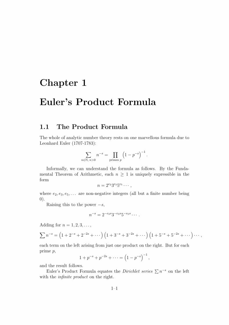
Chapter 1 Euler’s Product Formula 1.1 The Product Formula The whole of analytic number theory rests on one marvellous formula due to Leonhard Euler (1707-1783): n∈N, n>0 n -s = primes p 1 - p -s -1 . Informally, we can understand the formula as follows. By the Funda- mental Theorem of Arithmetic, each n ≥ 1 is uniquely expressible in the form n =2 e 2 3 e 3 5 e 5 ··· , where e 2 ,e 3 ,e 5 ,... are non-negative integers (all but a finite number being 0). Raising this to the power -s, n -s =2 -e 2 s 3 -e 3 s 5 -e 5 s ··· . Adding for n =1, 2, 3,... , n -s = 1+2 -s +2 -2s + ··· 1+3 -s +3 -2s + ··· 1+5 -s +5 -2s + ··· ··· , each term on the left arising from just one product on the right. But for each prime p, 1+ p -s + p -2s + ··· = 1 - p -s -1 , and the result follows. Euler’s Product Formula equates the Dirichlet series ∑ n -s on the left with the infinite product on the right. 1–1
Transcript of Chapter 1 Euler’s Product Formula - Trinity College, Dublin · Chapter 1 Euler’s Product...
Chapter 1
Euler’s Product Formula
1.1 The Product Formula
The whole of analytic number theory rests on one marvellous formula due toLeonhard Euler (1707-1783):
∑n∈N, n>0
n−s =∏
primes p
(1− p−s
)−1.
Informally, we can understand the formula as follows. By the Funda-mental Theorem of Arithmetic, each n ≥ 1 is uniquely expressible in theform
n = 2e23e35e5 · · · ,
where e2, e3, e5, . . . are non-negative integers (all but a finite number being0).
Raising this to the power −s,
n−s = 2−e2s3−e3s5−e5s · · · .
Adding for n = 1, 2, 3, . . . ,∑n−s =
(1 + 2−s + 2−2s + · · ·
) (1 + 3−s + 3−2s + · · ·
) (1 + 5−s + 5−2s + · · ·
)· · · ,
each term on the left arising from just one product on the right. But for eachprime p,
1 + p−s + p−2s + · · · =(1− p−s
)−1,
and the result follows.Euler’s Product Formula equates the Dirichlet series
∑n−s on the left
with the infinite product on the right.
1–1
1.2. INFINITE PRODUCTS 1–2
To make the formula precise, we must develop the theory of infinite prod-ucts, which we do in the next Section.
To understand the implications of the formula, we must develop the the-ory of Dirichlet series, which we do in the next Chapter.
1.2 Infinite products
1.2.1 Definition
Infinite products are less familiar than infinite series, but are no more com-plicated. Both are examples of limits of sequences.
Definition 1.1. The infinite product∏n∈N
cn
is said to converge to ` 6= 0 if the partial products
Pn =∏
0≤m≤n
cm → ` as n→∞.
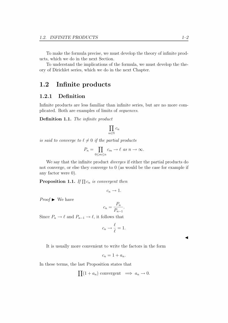
We say that the infinite product diverges if either the partial products donot converge, or else they converge to 0 (as would be the case for example ifany factor were 0).
Proposition 1.1. If∏cn is convergent then
cn → 1.
Proof I We have
cn =Pn
Pn−1
.
Since Pn → ` and Pn−1 → `, it follows that
cn →`
`= 1.
J
It is usually more convenient to write the factors in the form
cn = 1 + an.
In these terms, the last Proposition states that∏(1 + an) convergent =⇒ an → 0.
1.2. INFINITE PRODUCTS 1–3
1.2.2 The complex logarithm
The theory of infinite products requires some knowledge of the complex log-arithmic function.
Suppose z 6= 0. Letz = reiθ,
where r > 0. We are interested in solutions w ∈ C of
ew = z.
If w = x+ iy then
ex = r, e−iy = e−iθ,
ie
x = log r, y = θ + 2nπ
for some n ∈ Z.Just one of these solutions to ew = z satisfies
−π < y = =(w) ≤ π.
We call this value of w the principal logarithm of z, and denote it by Log z.Thus
eLog z = z, −π < =(z) ≤ π.
The general solution of ew = z is
w = Log z + 2nπi (n ∈ Z).
Now supposew1 = Log z1, w2 = Log z2.
Thenew1+w2 = z1z2 = eLog(z1z2)
It follows thatLog(z1z2) = Log z1 + Log z2 + 2nπi,
where it is easy to see that n = 0,−1 or 1.If <(z) > 0 then z = reiθ with −π/2 < θ < π/2. It follows that
<(z1),<(z2) > 0 =⇒ −π/2 < =(Log z1),=(Log z2) < π/2;
and so−π < =(Log z1 + Log z2) < π.
Thus<(z1),<(z2) > 0 =⇒ Log(z1z2) = Log z1 + Log z2.
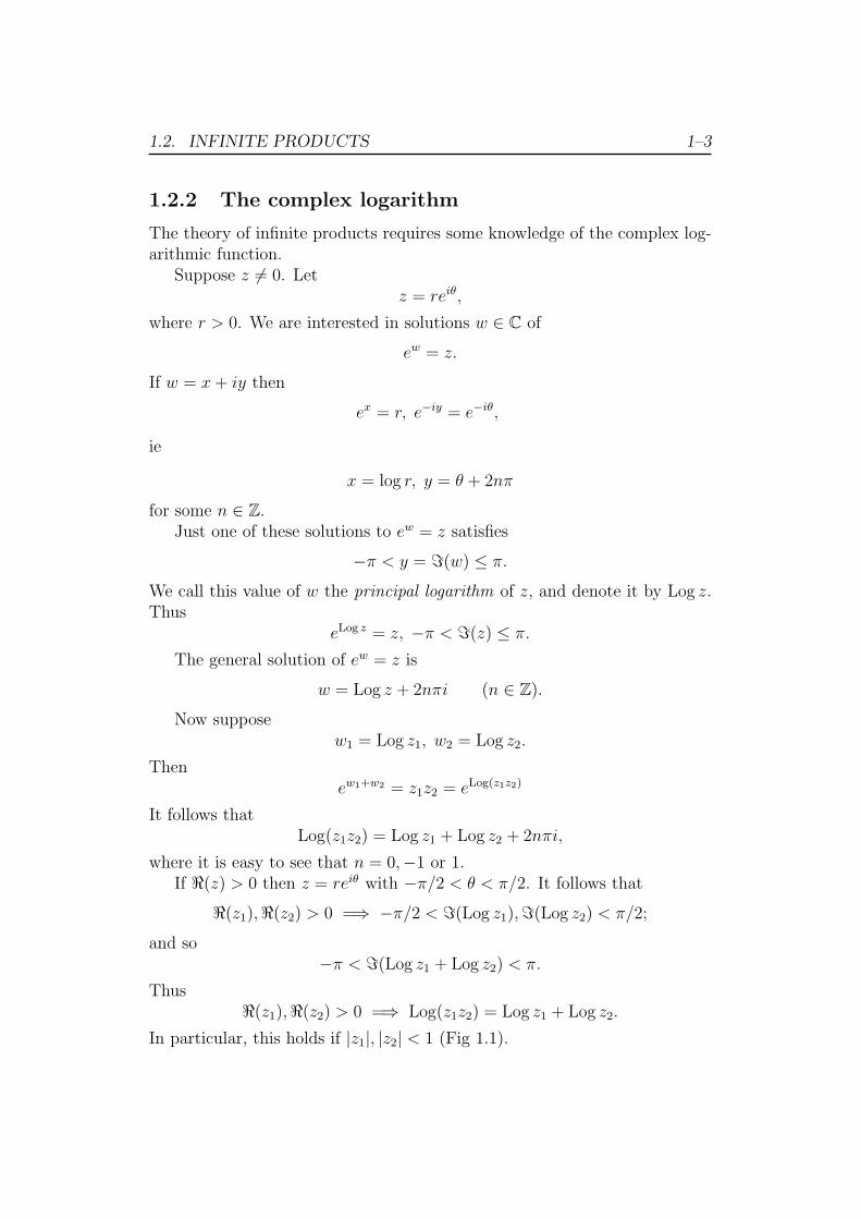
In particular, this holds if |z1|, |z2| < 1 (Fig 1.1).
1.2. INFINITE PRODUCTS 1–4
z
r
θ
1
Figure 1.1: |z − 1| < 1, Log z = log r + iθ
1.2.3 Convergence
Proposition 1.2. Suppose an 6= −1 for n ∈ N. Then∏(1 + an) converges ⇐⇒
∑Log(1 + an) converges.
Proof I Suppose∑
Log(1 + an) converges to S. Let
Sn =∑m≤n
Log(1 + am).
TheneSn =
∏m≤n
(1 + am).
ButSn → S =⇒ eSn → eS.
Thus∏
(1 + an) converges to es.Conversely, suppose
∏(1 + an) converges. Let
Pn =∏
m≤N
(1 + an).
Given ε > 0 there exists N such that
| Pn
Pm
− 1| < ε
if m,n ≥ N .
1.2. INFINITE PRODUCTS 1–5
It follows that if m,n ≥ N then
Log(Pn/PN) = Log(Pm/PN) + Log(Pn/Pm).
In particular (taking m = n− 1),
Log(Pn/PN) = Log(Pn−1/PN) + Log(1 + an).
HenceLog(Pn/PN) =
∑N<m≤m
Log(1 + am).
SincePn → ` =⇒ Log(Pn/LN)→ Log(`/PN),
we conclude that∑
n>N(1 + an) converges to Log(`/PN); and in particular,∑n≥0 Log(1 + an) is convergent. J
Proposition 1.3. Suppose an 6= −1 for n ∈ N. Then∑|an| convergent =⇒
∏(1 + an) convergent.
Proof I The function Log(1 + z) is holomorphic in |z| < 1, with Taylorexpansion
Log(1 + z) = z − z2/2 + z3/3− · · · .
Thus if |z| < 1/2 then
|Log(1 + z)| ≤ |z|+ |z|2 + |z|3 + · · ·
=|z|
1− |z|≤ 2|z|.
Now suppose∑|an| converges. Then an → 0; and so
|an| ≤ 1/2
for n ≥ N . It follows that
|Log(1 + an)| ≤ 2|an|
for n ≥ N . Hence ∑Log(1 + an) converges.
J
1.3. PROOF OF THE PRODUCT FORMULA 1–6
1.3 Proof of the product formula
Proposition 1.4. For <(s) > 1,∑n∈N, n>0
n−s =∏
primes p
(1− p−s
)−1,
in the sense that each side converges to the same value.
Proof I Let σ = <(s). Then
|n−s| = n−σ.
Thus
|N∑
M+1
n−s| ≤N∑
M+1
n−σ.
Nown−σ ≤
∫ n
n−1x−σdx;
and soN∑
M+1
n−σ ≤∫ N
Mx−σdx
=1
σ
(M−σ −N−σ
)→ 0 as M,N →∞.
Hence∑n−s is convergent, by Cauchy’s criterion.
On the other hand, ∏(1− p−s)
is absolutely convergent, since∑|p−s| =
∑p−σ ≤
∑n−σ,
which we just saw is convergent. Hence∏
(1− p−s) is convergent, by Propo-sition 1.3; and so therefore is ∏(
1− p−s)−1
.
To see that the two sides are equal note that∏p≤N
(1− χ(p)p−s
)−1=∑n≤N
χ(n)n−s +′∑χ(n)n−s,
where the second sum on the right extends over those n > N all of whoseprime factors are ≤ N .
As N → ∞, the right-hand side → ∑n−s, since this sum is absolutely
convergent; while by definition, the left-hand side → ∏(1 − p−s)−1. We
conclude that the two sides converge to the same value. J
1.4. EULER’S THEOREM 1–7
1.4 Euler’s Theorem
Proposition 1.5. (Euler’s Theorem)
∑primes p
1
p=∞.
Proof I Suppose∑
1/p is convergent. Then
∏(1− 1
p
)
is absolutely convergent, and so converges to ` say, by Proposition ?? Itfollows that ∏
p≤N
(1− 1
p
)→ `−1.
ButN∑1
1
n≤∏
p≤N
(1− 1
p
),
since each n on the left is expressible in the form
n = pe11 · · · per
r
with p1, . . . , pr ≤ N .Hence
∑1/n is convergent. But
1
n>∫ n+1
n
dx
x.
ThusN∑1
n−1 ≥∫ N+1
1
dx
x= log(N + 1).
Since logN →∞ as N →∞ it follows that∑
1/n is divergent.Our hypothesis is therefore untenable, and
∑ 1
pdiverges.
J
This is a remarkably accurate result;∑ 1
ponly just diverges. For it follows
from the Prime Number Theorem,
π(x) ∼ x
log x,
1.4. EULER’S THEOREM 1–8
that if pn denotes the nth prime (so that p2 = 3, p5 = 11, etc) then
pn ∼ n log n.
To see that, note that π(pn) = n (ie the number of primes ≤ pn is n).Thus setting x = pn in the Prime Number Theorem,
n ∼ pn
log pn
,
ie
pn
n log pn
→ 1.
Taking logarithms,
log pn − log n− log log pn → 0;
hence
log n
log pn
→ 1,
ie
log pn ∼ log n.
We conclude thatpn ∼ n log pn ∼ n log n.
Returning to Euler’s Theorem, we see that∑
1/p behaves like∑
1/n log n.The latter diverges, but only just, as we see by comparison with∫ dx
x log x= log log x.
On the other hand, ∑p
1
p logε p
converges for any ε > 0, since ∑n
1
n log1+ε n
converges by comparison with∫ dx
x log1+ε x= −1
εlog−ε x.
What is perhaps surprising is that it is so difficult to pass from Euler’sTheorem to the Prime Number Theorem.
Chapter 2
Dirichlet series
2.1 Definition
Definition 2.1. A Dirichlet series is a series of the form
a11−s + a22
−s + a33−s + · · · ,
where ai ∈ C.
Remarks. 1. For n ∈ N we set
n−s = e−s log n,
taking the usual real-valued logarithm. Thus n−s is uniquely definedfor all s ∈ C. Moreover,
m−sn−s = (mn)−s, n−sn−s′ = n−(s+s′);
while1−s = 1
for all s.
2. The use of −s rather than s is simply a matter of tradition. The seriesmay of course equally well be written
a1 +a2
2s+a3
3s+ · · · .
3. The term ‘Dirichlet series’ is often applied to the more general series
a0λ−s0 + a1λ
−s1 + a2λ
−s2 + · · · ,
2–1
2.2. CONVERGENCE 2–2
where0 < λ0 < λ1 < λ2 < · · · ,
andλ−s = e−s log λ
Such series often appear in mathematical physics, where the λi mightbe, for example, the eigenvalues of an elliptic operator. However, weshall only make use of Dirichlet series of the more restricted type de-scribed in the definition above; and we shall always use the term inthat sense, referring to the more general series (if at all) as generalisedDirichlet series.
4. It is perhaps worth noting that generalised Dirichlet series includepower series
f(x) =∑
cnxn,
in the sense that if we make the substitution x = e−s then
f(e−s) =∑
cne−ns =
∑cn(en)−s.
2.2 Convergence
Proposition 2.1. Suppose
f(s) = a11−s + a22
−s + · · ·
converges for s = s0. Then it converges for all s with
<(s) > <(s0).
Proof I We use a technique that might be called ‘summation by parts’, byanalogy with integration by parts.
Lemma 1. Suppose an, bn(n ∈ N) are two sequences. Let
An =∑m≤n
am, Bn =∑m≤n
bm.
ThenN∑M
anBn = ANBN+1 − AM−1BM −N∑M
Anbn+1.
2.2. CONVERGENCE 2–3
Proof I Substituting an = An − An−1,
N∑M
anBn =N∑M
(An − An−1)Bn
=N∑M
An(Bn −Bn+1) + ANBN+1 − AM−1BM
= −N∑M
Anbn+1 + ANBN+1 − AM−1BM .
J
Lemma 2. Suppose∑an converges and
∑bn converges absolutely. Then∑
anBn
converges.
Proof I By the previous Lemma,
N∑M
anBn = ANBN+1 − AM−1BM −N∑M
Anbn+1
= AN(BN+1 −BM) + (AN − AM−1)BM −N∑M
Anbn+1.
Let∑an = A,
∑bn = B. The partial sums of both series must be
bounded; say|An| ≤ C, |Bn| ≤ D.
Then
|N∑M
anBn| ≤ C|BN+1 −BM |+D|AN − AM−1|+ CN∑M
|bn+1|.
As M,N →∞,
BN+1 −BM → 0, AN − AM−1 → 0,N∑M
|bn+1| → 0.
HenceN∑M
anBn → 0
as M,N →∞; and therefore∑anBn converges, by Cauchy’s criterion. J
2.2. CONVERGENCE 2–4
Let s′ = s− s0. Then <(s′) > 0. We apply the last Lemma with ann−s0
for an, and n−s′ for Bn. Thus
bn = Bn −Bn−1
= n−s′ − (n− 1)−s′
= −s′∫ n
n−1x−s′ dx
x.
Hence
|bn| ≤ |s′|∫ n
n−1|x−s′|dx
x
= |s′|∫ n
n−1x−σ′ dx
x,
where σ′ = <(s′).Summing,
N∑M
|bn| ≤ |s′|∫ N
M−1x−σ′ dx
x
=|s′|σ′
((M − 1)−σ′ −N−σ′
).
It follows thatN∑M
|bn| → 0 as M,N →∞.
Thus∑|bn| is convergent, and so the conditions of the last Lemma are
fulfilled. We conclude that∑ann
−s0n−s′ =∑
ann−(s0+s′) =
∑ann
−s
is convergent. J
Corollary 2.1. A Dirichlet series either
1. converges for all s,
2. diverges for all s, or
3. converges for all s to the right of a line
<(s) = σ0,
and diverges for all s to the left of this line.
2.3. ABSOLUTE CONVERGENCE 2–5
σ0 Xσ
σ + iT X + iT
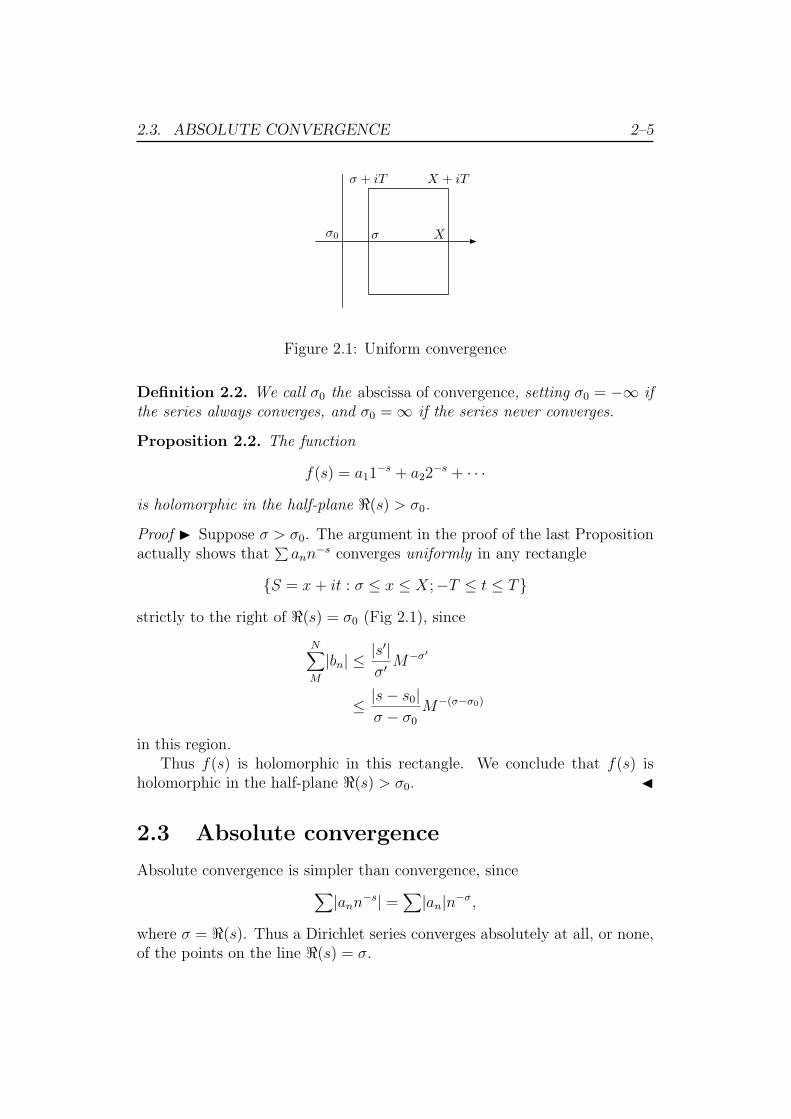
Figure 2.1: Uniform convergence
Definition 2.2. We call σ0 the abscissa of convergence, setting σ0 = −∞ ifthe series always converges, and σ0 =∞ if the series never converges.
Proposition 2.2. The function
f(s) = a11−s + a22
−s + · · ·
is holomorphic in the half-plane <(s) > σ0.
Proof I Suppose σ > σ0. The argument in the proof of the last Propositionactually shows that
∑ann
−s converges uniformly in any rectangle
{S = x+ it : σ ≤ x ≤ X;−T ≤ t ≤ T}
strictly to the right of <(s) = σ0 (Fig 2.1), since
N∑M
|bn| ≤|s′|σ′M−σ′
≤ |s− s0|σ − σ0
M−(σ−σ0)
in this region.Thus f(s) is holomorphic in this rectangle. We conclude that f(s) is
holomorphic in the half-plane <(s) > σ0. J
2.3 Absolute convergence
Absolute convergence is simpler than convergence, since∑|ann
−s| =∑|an|n−σ,
where σ = <(s). Thus a Dirichlet series converges absolutely at all, or none,of the points on the line <(s) = σ.
2.3. ABSOLUTE CONVERGENCE 2–6
Proposition 2.3. If
f(s) = a11−s + a22
−s + · · ·
converges absolutely for s = s0 then it converges absolutely for all s with
<(s) ≥ <(s0).
Proof I This follows at once from the fact that each term
|ann−s| = |an|n−σ
is a decreasing function of σ. J
Corollary 2.2. A Dirichlet series either
1. converges absolutely for all s,
2. does not converge absolutely for any s, or
3. converges absolutely for all s to the right of a line
<(s) = σ1,
and does not converge absolutely for any s to the left of this line.
Definition 2.3. We call σ1 the abscissa of absolute convergence, settingσ1 = −∞ if the series always converges absolutely, and σ1 =∞ if the seriesnever converges absolutely.
Proposition 2.4. We have
σ0 ≤ σ1 ≤ σ0 + 1.
Proof I Suppose<(s) > σ0.
Thenf(s) = a11
−s + a22−s + · · ·
is convergent. Henceann
−s → 0 as n→∞.
In particular, ann−s is bounded, say
|ann−s| ≤ C.
2.4. THE RIEMANN ZETA FUNCTION 2–7
But then|ann
−(s+1+ε)| ≤ Cn−(1+ε)
for any ε < 0. Since∑n−(1+ε) converges, it follows that
f(s+ 1 + ε)
converges absolutely. We have shown therefore that
σ > σ0 =⇒ σ + 1 + ε ≥ σ1
for any ε > 0, from which it follows that
σ0 + 1 ≥ σ1.
J
Proposition 2.5. If an ≥ 0 then σ1 = σ0.
Proof I This is immediate, since in this case∑|ann
−σ| =∑
ann−σ.
J
2.4 The Riemann zeta function
Although we have already met the function ζ(s), it may be best to give aformal definition.
Definition 2.4. The Riemann zeta function ζ(s) is defined by the Dirichletseries
ζ(s) = 1−s + 2−s + · · · .
Remarks. 1. We shall often refer to the Riemann zeta function ζ(s) simplyas the zeta function. This is slightly inaccurate, since the term ‘zetafunction’ is applied to a wide range of related functions. However, theRiemann zeta function is the only such function we shall use; so itwill cause no confusion if we use the unadorned term ‘zeta function’ todescribe it.
2. For example, there is a zeta function ζk(s) corresponding to each num-ber field k, defined by
ζk(s) =∑a
N(a)−s,
2.4. THE RIEMANN ZETA FUNCTION 2–8
where a runs over the ideals in k (or rather, in the ring of integersI(k) = k ∩ Z), and N(a) is the number of residue classes moda.
Since the unique factorisation theorem holds for ideals, the analogue ofEuler’s product formula holds:
ζk(s) =∏p
(1−N(p)−s
)−1,
where the product runs over all prime ideals in I(k).
This allows the Prime Number Theorem to be extended to give anapproximate formula for the number of prime ideals p in the numberfield k with N(p) ≤ n.
3. In another direction, the zeta function ζE(s) of an elliptic differential(or pseudo-differential) operator E is defined by
ζE(s) =∑
λ−sn ,
where λn (n = 0, 1, 2, . . . ) are the eigenvalues of E (necessarily positive,if E is elliptic).
The Riemann zeta function ζ(s) can be interpreted in this sense as thezeta function of the Laplacian operator on the circle S1.
Proposition 2.6. The abscissa of convergence of the Riemann zeta functionis
σ0 = 1.
Proof I This follows at once from the fact that∑n−σ <∞ ⇐⇒ σ > 1.
Let us recall how this is established, by comparing the sum with theintegral
∫x−σdx. If n− 1 ≤ x ≤ n,
n−σ ≤ x−σ ≤ (n− 1)−σ.
Integrating,
n−σ <∫ n
n−1x−σdx < (n− 1)−σ,
Summing from n = M + 1 to N ,
N∑M+1
n−σ <∫ N
Mx−σdx <
N+1∑M
n−σ,
2.4. THE RIEMANN ZETA FUNCTION 2–9
It follows that∑n−σ and
∫∞ x−σdx converge or diverge together.But we can compute the integral directly: if n = 1 then∫ Y
Xx−1dx = logX − log Y,
and so the integral diverges; while if n 6= 1 then∫ Y
Xx−σdx =
1
σ − 1(M1−σ −N1−σ),
and so the integral converges if σ > 1 and diverges if σ < 1. J
Corollary 2.3. The zeta function ζ(s) is holomorphic in the half-plane<(s) > 1.
We can continue ζ(s) analytically to the half-plane <(s) > 0 in the fol-lowing way.
Proposition 2.7. The Dirichlet series
f(s) = 1−s − 2−s + 3−s − · · ·has abscissa of convergence σ0 = 0, and so defines a holomorphic functionin the half-plane <(s) > 0.
Proof I Suppose σ > 0. Then
f(σ) = 1−σ − 2−σ + 3−σ − · · ·converges, since the terms alternate in sign and decrease to 0 in absolutevalue. It follows, by Proposition 2.1, that f(s) converges for <(s) > 0.
The series certainly does not converge for <(s) < 0, since the terms donot even → 0. Thus σ0 = 0. J
The abscissa of absolute convergence σ1 of f(s) is 1 since the terms havethe same absolute value as those of ζ(s).
Proposition 2.8. If <(s) > 1 then
f(s) = (1− 21−s)ζ(s).
Proof I If <(s) > 1 then the Dirichlet series for f(s) converves absolutely,so we may re-arrange its terms:
f(s) = 1−s − 2−s + 3−s − · · ·= (1−s + 2−s + 3−s + · · · )− 2(2−s + 4−s + · · · )= ζ(s)− 2 · 2−s(1−s + 2−s + · · · )= ζ(s)− 2 · 2−sζ(s)
= (1− 21−s)ζ(s).
J
2.4. THE RIEMANN ZETA FUNCTION 2–10
Proposition 2.9. The zeta function ζ(s) extends to a meromorphic functionin <(s) > 0, with a single simple pole at s = 1 with residue 1.
Proof I We have
ζ(s) =1
1− 21−sf(s)
for <(s) > 1. But the right-hand side is meromorphic in <(s) > 0, and sodefines an analytic continuation of ζ(s) (necessarily unique, by the theory ofanalytic continuation) to this half-plane.
Since f(s) is holomorphic in this region, any pole of ζ(s) must be a poleof 1/(1− 21−s), ie a zero of 1− 21−s. But
21−s = e(1−s) log 2.
Hence21−s = 1 ⇐⇒ (1− s) log 2 = 2nπi
for some n ∈ Z. Thus 1/(1− 21−s) has poles at
s = 1 +2nπ
log 2i (n ∈ Z).
At first sight this seems to give an infinity of poles of ζ(s) on the line<(s) = 1. However, the following argument shows that f(s) must vanish atall these points except s = 1, thus ‘cancelling out’ all the poles of 1/(1−21−s)except that at s = 1.
Consider
g(s) = 1−s + 2−s − 2 · 3−s + 4−s + 5−s − 2 · 6−s + · · · .
Like f(s), this converges for all σ > 0. For if we group g(σ) in sets of threeterms
g(σ) = (1−σ + 2−σ − 2 · 3−σ) + (4−σ + 5−σ − 2 · 6−σ) + · · ·
we see that each set is > 0. Thus the series either converges (to a limit > 0),or else diverges to +∞.
On the other hand, we can equally well group g(σ) as
g(σ) = 1−σ + 2−σ − (2 · 3−σ − 4−σ − 5−σ)− (2 · 6−σ − 7−σ − 8−σ) + · · · .
Now each group is < 0, if we omit the terms 1−σ + 2−σ. Thus g(σ) eitherconverges (to a limit < 1−σ + 2−σ), or else diverges to −∞.
We conclude the g(σ) converges (to a limit between 0 and 1−σ + 2−σ).
2.4. THE RIEMANN ZETA FUNCTION 2–11
Hence g(s) converges for <(s) > 0.But if <(s) > 1 we can re-write g(s) as
g(s) = (1−s + 2−s + 3−s + · · · )− 3(3−s + 6−s + 9−s + · · · )= (1− 31−s)ζ(s).
Thus
ζ(s) =1
1− 31−sg(s).
The right hand side is meromorphic in the half-plane <(s) > 0, giving asecond analytic continuation of ζ(s) to this region, which by the theory ofanalytic contination must coincide with the first.
But the poles of 1/(1− 31−s) occur where
(1− s) log 3 = 2mπi,
ie
s = 1 +2πm
log 3i.
Thus ζ(s) can only have a pole where s is expressible in both forms
s = 1 +2πn
log 2i = 1 +
2πm
log 3i (m,n ∈ Z).
But this implies that
m log 2 = n log 3,
ie
2m = 3n,
which is of course impossible (by the Fundamental Theorem of Arithmetic)unless m = n = 0.
We have therefore eliminated all the poles except s = 1. At s = 1,
f(1) = 1− 1
2+
1
3− 1
4+ · · · = log 2.
(This follows on letting x → 1 from below in log(1 + x) = x − x2/2 + · · · .)On the other hand, if we set s = 1 + s′ then
1− 21−s = 1− e−s′ log 2
= s′ log 2− s′2/2! log2 2 + · · ·= s′ log 2(1− s′/2 log 2 + · · ·
2.5. THE RIEMANN-STIELTJES INTEGRAL 2–12
Thus
1
1− 21−s=
1
1− 2−s′
=1
log 2 s′(1 +
s′
2log 2 + · · · )
=1
log 2 s′+ h(s),
where h(s) is holomorphic. Hence
ζ(1 + s′) =1
s′+ h(s)f(s).
We conclude that ζ(s) has a simple pole at s = 1 with residue 1. J
In Chapter 7 we shall see that ζ(s) can in fact be analytically continuedto the whole of C. It has no further poles; its only pole is at s = 1.
2.5 The Riemann-Stieltjes integral
It is helpful (although by no means essential) to introduce a technique whichallows us to express sums as integrals, and brings ‘summation by parts’ intothe more familiar guise of integration by parts.
Let us recall the definition of the Riemann integral∫ ba f(x) dx of a contin-
uous function f(x) on [a, b]. Note that f(x) is in fact uniformly continuouson [a, b], ie given ε > 0 there exists a δ > 0 such that
|x− y| < δ =⇒ |f(x)− f(y)| < ε
for x, y ∈ [a, b].By a dissection ∆ of [a, b] we mean a sequence
∆ : a = x0 < x1 < · · · < xn = b.
We set‖∆‖ = max
0≤i<n|xi+1 − xi|.
The dissection ∆′ is said to be a refinement of ∆, and we write ∆′ ⊂ ∆ ifthe set of dissection-points xi of ∆ is a subset of the set of dissection-pointsof ∆′. Evidently
∆′ ⊂ ∆ =⇒ ‖∆′‖ ≤ ‖∆‖.
2.5. THE RIEMANN-STIELTJES INTEGRAL 2–13
LetS(f,∆) =
∑0≤i<n
f(xi)(xi+1 − xi).
Then S(f,∆) is convergent as ‖∆‖ → 0, ie given ε > 0 there exists δ > 0such that
‖∆1‖, ‖∆2‖ < δ =⇒ |S(f,∆1)− S(f,∆2)| < ε.
This follows from 2 lemmas (each more or less immediate).
1. Suppose|x− y| < δ =⇒ |f(x)− f(y)| < ε.
Then
‖∆1‖ < δ, ∆2 ⊂ ∆ =⇒ |S(f,∆1)− S(f,∆2)| < (b− a)ε.
2. Given 2 dissections ∆1,∆2 of [a, b] we can always find a common re-finement ∆3, ie
∆3 ⊂ ∆1, ∆3 ⊂ ∆2.
These in turn imply
3.‖∆1‖, ‖∆2‖ < δ =⇒ |S(f,∆1)− S(f,∆2)| < 2(b− a)ε.
Thus, by Cauchy’s criterion, S(f,∆) converges as ∆→ 0, ie there exists anI ∈ C such that ie given ε > 0 there exists δ > 0 such that
|S(f,∆)− I| < ε if ‖∆‖ < δ.
Even if f(x) is not continuous, we say that it is Riemann-integrable on[a, b] with ∫ b
af(x) dx = I
ifS(f,∆)→ I as ‖∆‖ → 0.
Now suppose M(x) is an increasing (but not necessarily strictly increas-ing) function on [a, b], ie
x ≤ y =⇒ f(x) ≤ f(y).
Then we set
SM(f,∆) =∑
0≤i<n
f(xi)(M(xi+1)−M(xi)).
2.5. THE RIEMANN-STIELTJES INTEGRAL 2–14
Proposition 2.10. If f(x) is continuous and M(x) is increasing then
SM(f,∆) converges as ‖∆‖ → 0.
Proof I The result follows in exactly the same way as for the Riemann in-tegral above, with (1) replaced by
1’. Given ε > 0, suppose δ > 0 is such that
|x− y| < δ =⇒ |f(x)− f(y)| < ε.
Then if ‖∆1‖, ‖∆2‖ < δ,
|S(f,∆1)− S(f,∆2)| < (M(b)−M(a))ε.
J
Definition 2.5. We call
I = lim‖∆‖→0
SM(f,∆)
the Riemann-Stieltjes integral of f(x) with respect to M(x), and write∫ b
af(x) dM = I.
2.5.1 Functions of bounded variation
Definition 2.6. A (real- or complex-valued) function f(x) is said to be ofbounded variation on the interval [a, b] if there exists a constant C such that
A(f,∆) =∑|f(xi)− f(xi−1)| ≤ C
for all dissections ∆ of [a, b].
Proposition 2.11. Any linear combination
f(x) = µ1f1(x) + · · ·+ µrfr(x) (µ1, . . . , µr ∈ C)
of functions f1(x), . . . , fr(x) of bounded variation is itself of bounded varia-tion.
Proof I This follows at once from the fact that
A(f,∆) ≤ |µ1|A(f1,∆) + · · ·+ |µr|A(fr,∆).
J
2.5. THE RIEMANN-STIELTJES INTEGRAL 2–15
Proposition 2.12. Any monotone increasing or decreasing function f(x) isof bounded variation.
Proof I If f(x) is increasing then
|f(xi)− f(xi−1| = f(xi)− f(xi−1;
and soA(f,∆) = f(b)− f(a).
If f(x) is decreasing then −f(x) is increasing, so the result follows from thelast Proposition. J
Proposition 2.13. A function f(x) of class C1[a, b], ie with continuousderivative f ′(x) on [a, b], is of bounded variation.
Proof I Since f ′(x) is continuous, it is bounded: say
|f ′(x)| ≤ C.
Also, by the Mean Value Theorem,
f(xi)− f(xi−1 = (xi − xi−1)f′(ξ),
where xi−1 < ξ < xi. Hence
|f(xi)− f(xi−1| ≤ C(xi − xi−1);
and soA(f,∆) ≤ C(b− a).
J
Proposition 2.14. A real-valued function f(x) is of bounded variation on[a, b] if and only if it can be expressed as the difference of two increasingfunctions:
f(x) = M(x)−N(x),
where M(x), N(x) are monotone increasing.
Proof I If f(x) is expressible in this form then it is of bounded variation,by Propositions 2.12 and 2.11.
For the converse, let
P (f,∆) =∑
i:f(xi)≥f(xi−1)
(f(xi)− f(xi−1)),
N(f,∆) = −∑
i:f(xi)<f(xi−1)
(f(xi)− f(xi−1)).
2.5. THE RIEMANN-STIELTJES INTEGRAL 2–16
for each dissection ∆ of [a, b]. Then P (f,∆), N(f,∆) ≥ 0; and
P (f,∆)−N(f,∆) = f(b)− f(a), P (f,∆) +N(f,∆) = A(f,∆).
It follows that0 ≤ P (f,∆), N(f,∆) ≤ A(f,∆).
HenceP (f) = sup
∆P (f,∆), N(f) = sup
∆N(f,∆)
are defined.
Lemma 3. We have
P (f)−N(f) = f(b)− f(a).
Proof I Given ε > 0 we can find dissections ∆1,∆2 such that
P (f) ≥ P (f,∆1) > P (f)− ε,N(f) ≥ N(f,∆2) > N(f)− ε.
If now ∆ is a common refinement of ∆1,∆2 then
P (f) ≥ P (f,∆) ≥ P (f,∆1) > P (f)− ε,N(f) ≥ N(f,∆) ≥ N(f,∆2) > N(f)− ε.
ButP (f,∆)−N(f,∆) = f(b)− f(a).
It follows that
P (f)−N(f)− ε ≤ f(b)− f(a) ≤ P (f)−N(f) + ε.
Since this is true for all ε > 0,
P (f)−N(f) = f(b)− f(a).
J
Now suppose a ≤ x ≤ b. We apply the argument above to the interval[a, x]. Let p(x), n(x) be the functions P (f), N(f) for the interval [a, x]. Bythe last Lemma,
p(x)− n(x) = f(x)− f(a).
It is easy to see that p(x), n(x) are increasing functions of x. For suppose
a ≤ x < y ≤ b.
2.5. THE RIEMANN-STIELTJES INTEGRAL 2–17
To each dissection∆ : a = x0 < x1 < · · ·xn = x
of [a, x] we can associate the dissection
∆′ : a = x0 < x1 < · · ·xn < xn+1 = y
of [a, y]; and then
P (f,∆′) ≥ P (f,∆), N(f,∆′) ≥ N(f,∆).
It follows thatp(y) ≥ p(x), n(y) ≥ n(x),
ie p(x), n(x) are monotone increasing. Since
f(x) = (f(a) + p(x))− n(x),
this establishes the result. J
Proposition 2.15. The function f(x) is of bounded variation on [a, b] if andonly if it can be expressed as a linear combination of increasing functions:
f(x) = µ1M1(x) + · · ·+ µrMr(x),
where M1(x), . . . ,Mr(x) are monotone increasing, and µ1, . . . , µr ∈ C.
Proof I It follows from Propositions 2.11 and 2.12 that a function of thisform is of bounded variation.
For the converse, note that if f(x) is complex-valued then it can be splitinto its real and imaginary parts:
f(x) = fR(x) + ifI(x)
where fR(x), fI(x) are real-valued functions. It is easy to see that if f(x) isof bounded variation then so are fR(x) and fI(x). Hence each is expressibleas a difference of increasing functions, say
fR(x) = MR(x)−NR(x), fI(x) = MI(x)−NI(x).
But thenf(x) = MR(x)−NR(x) + iMI(x)− iNI(x),
which is of the required form. J
2.5. THE RIEMANN-STIELTJES INTEGRAL 2–18
This result allows us to extend the Riemann-Stieltjes integral to functionsof bounded variation.
Suppose U(x) is a function of bounded variation on [a, b]. We set
SU(f,∆) =∑
f(xi)(U(xi+1)− U(xi))
for any dissection ∆ of [a, b].
Proposition 2.16. If f(x) is continuous and U(x) is of bounded variationthen
SU(f,∆) converges as ‖∆‖ → 0.
Proof I By the last Proposition, we can express U(x) as a linear combinationof increasing functions. The result then follows from Proposition 2.10. J
Definition 2.7. We call
I = lim‖∆‖→0
SU(f,∆)
the Riemann-Stieltjes integral of f(x) with respect to U(x), and write∫ b
af(x) dU = I.
We extend the Riemann-Stieltjes integral to non-continuous functionsf(x) as we do the familiar Riemann integral. Thus if
SU(f,∆)→ I as ‖∆‖ → 0
then we say that f(x) is Riemann-Stieltjes integrable on [a, b], with∫ b
af(x) dU = I.
Similarly, we extend the Riemann-Stieltjes integral to infinite ranges inthe same was as the Riemann integral. Thus we set∫ ∞
af(x)dU = lim
X→∞
∫ X
af(x)dU,
if the limit exists.In one important case the Riemann-Stieltjes integral reduces to the fa-
miliar Riemann integral.
2.5. THE RIEMANN-STIELTJES INTEGRAL 2–19
Proposition 2.17. Suppose U(x) is of class C1[a, b], ie U(x) has continuousderivative U ′(x) on [a, b]; and suppose f(x)U ′(x) is Riemann integrable on[a, b]. Then f(x) is Riemann-Stieltjes integrable, and∫ b
af(x)dU =
∫ b
af(x)U ′(x)dx.
Proof I Suppose ∆ is a dissection of [a, b]. We compare SU(f,∆) withS(fU ′,∆).
By the Mean Value Theorem,
U(xi+1)− U(xi) = U ′(ξi)
where xi < ξi < xi+1. Moreover, since U ′(x) is continuous on [a, b], it isabsolutely continuous; so given any ε > 0 we can find δ > 0 such that
|U ′(xi)− U ′(ξi)| < ε
if xi+1 − xi < δ.Hence
|SU(f,∆)− S(fU ′,∆)| ≤ max|f |(b− a)ε
if ‖∆‖ < δ, from which the result follows. J
2.5.2 Discontinuities
Proposition 2.18. If f(x) is a function of bounded variation on [a, b] thenthe left limit
f(x− 0) = limt→x−0
f(t)
exists for all x ∈ [a, b); and the right limit
f(x+ 0) = limt→x+0
f(t)
exists for all x ∈ (a, b].
Proof I The result is (almost) immediate if f(x) is increasing. It follows forany function f(x) of bounded variation by Proposition 2.15, since
f(x) = µ1M1(x)+· · ·+µrMr(x) for all x =⇒ f(x−0) = µ1M1(x−0)+· · ·+µrMr(x−0),
and similarly for the right limit. J
2.5. THE RIEMANN-STIELTJES INTEGRAL 2–20
The function f(x) is continuous at x = ξ if
f(ξ − 0) = f(ξ) = f(ξ + 0).
Otherwise f(x) has a discontinuity at ξ.
Proposition 2.19. The discontinuities of a function f(x) of bounded vari-ation are enumerable.
Proof I It is sufficient to prove the result for an increasing function; for if
f(x) = µ1M1(x) + · · ·+ µrMr(x)
then the discontinuities of f(x) lie in the union of the discontinuities ofM1(x), . . . ,Mr(x); and a finite union of enumerable sets is enumerable.
Let us define the ‘jump’ at a discontinuity ξ to be
j(ξ) = f(ξ + 0)− f(ξ − 0).
Note that for an increasing function
f(ξ − 0) ≤ f(ξ) ≤ f(ξ + 0).
Thus f(x) is discontinuous at ξ if and only if j(ξ) > 0.
Lemma 4. Suppose M(x) is increasing on [a, b]; and suppose
a ≤ ξ1 < ξ2 < · · · < ξn ≤ b.
Then ∑1≤i≤n
j(ξi) ≤ f(b)− f(a).
Proof I Choose a dissection x0, x1, . . . , xn of [a, b] with
a = x0 ≤ ξ1 < x1 < ξ2 < x2 < · · · < xn−1 < ξn ≤ xn = b.
Then it is easy to see that
f(xi)− f(xi−1) ≥ j(ξi);
and so, on addition,f(b)− f(a) ≥
∑j(ξi).
J
2.5. THE RIEMANN-STIELTJES INTEGRAL 2–21
Corollary 2.4. Suppose M(x) is increasing on [a, b]; Then the number ofdiscontinuities with
j(x) = f(x+ 0)− f(x− 0) ≥ 2−r
is≤ 2r(f(b)− f(a)).
Using the Lemma, we can enumerate the discontinuities of M(x) by firstlisting those with j(x) ≥ 1, then those with 1 > j(x) ≥ 2−1, then those with2−1 > j(x) ≥ 2−2, and so on. In this way we enumerate all the discontinuities:
ξ0, ξ1, ξ2, . . . .
J
Remarks. 1. Note that we are not claiming that the discontinuities canbe enumerated in increasing order, ie so that
ξ0 < ξ1 < ξ2 < · · · .
That is not so, in general; f(x) could , for example, have a discontinuityat every rational point.
2. The discontinuity at ξ can be divided into two parts:
f(ξ)− f(ξ − 0) and f(ξ + 0)− f(ξ).
However, if f(x) is right-continuous, ie
f(x+ 0) = f(x)
for all x ∈ [a, b), then the second contribution vanishes, and the dis-continuity is completely determined by
j(ξ) = f(ξ + 0)− f(ξ − 0) = f(ξ)− f(ξ − 0).
To simplify the discussion, the functions we use have all been chosento be right-continuous; for example, we set
π(x) = ‖{p : p ≤ x}‖,
although we could equally well have taken the left-continuous function
π1(x) = ‖{p : p < x}‖.
2.5. THE RIEMANN-STIELTJES INTEGRAL 2–22
(From a theoretical point of view, it might have been preferable to haveimposed the symmetric condition
f(x) =1
2(f(x+ 0) + f(x− 0)) .
However, for our purposes the added complication would outweigh thetheoretical advantage.)
Definition 2.8. The step function Hξ(x) is defined by
Hξ(x) =
0 if x < ξ,
1 if x ≥ ξ.
Proposition 2.20. Suppose U(x) is a right-continuous function of boundedvariation on [a, b]. Then ∑
ξ
j(ξ)
is absolutely convergent.
Proof I It is sufficient to prove the result when U(x) is increasing, by Propo-sition 2.15. But in that case j(ξ) > 0, and∑
ξ
j(ξ) ≤ f(b)− f(a),
by Lemma 4. J
Proposition 2.21. Suppose U(x) is a right-continuous function of boundedvariation on [a, b]. Then U(x) can be split into two parts,
U(x) = J(x) + f(x),
where f(x) is continuous, and
J(x) =∑
j(ξ)Hξ(x),
the sum extending over all discontinuities ξ of f(x) in [a, b].
Proof I It is sufficient to prove the result in the case where U(x) is increas-ing, by Proposition 2.15.
Letf(x) = U(x)− J(x).
We have to show that f(x) is continuous.
2.5. THE RIEMANN-STIELTJES INTEGRAL 2–23
The step functionHξ(x) is right-continuous. Hence J(x) is right-continuous;and since U(x) is right-continuous by hypothesis, it follows that f(x) is right-continuous. We have to show that f(x) is also left-continuous.
Suppose x < y. Then
J(y)− J(x) =∑
x<ξ≤y
j(ξ)
≤ U(y)− U(x),
by Proposition 4. Thus
f(x) = U(x)− J(x) ≤ U(y)− J(y) = f(y),
ie f(x) is increasing.Moreover,
0 ≤ f(y)− f(x) ≤ U(y)− U(x).
Hence0 ≤ f(y)− f(y − 0) ≤ U(y)− U(y − 0).
In particular, if U(x) is left-continuous at y then so is f(x).Now suppose U(x) has a discontinuity at y. If x < y then
J(y)− J(x) ≥ j(y) = U(y)− U(y − 0).
Hence
J(y)− J(y − 0) ≥ U(y)− U(y − 0),
ie
f(y − 0) = U(y − 0)− J(y − 0) ≥ f(y) = U(y)− J(y).
Since f(x) is increasing, it follows that
f(y − 0) = f(y),
ie f(x) is left-continuous at y. J
Definition 2.9. We call f(x) the continuous part of U(x), and J(x) thepurely discontinous part.
Remarks. 1. This is our own terminology; there do not seem to be stan-dard terms for these two parts of a function of bounded variation. Thatis probably because they are more generally studied through the mea-sure or distribution dU , with the step function Hξ(x) replaced by theDirac delta ‘function’ δξ(x) = dHξ.
2.5. THE RIEMANN-STIELTJES INTEGRAL 2–24
2. Our definition of J(x) entails that J(a) = 0. With that condition, thesplitting of U(x) is unique. If we drop the condition then J(x) andf(x) are defined up to a constant.
Proposition 2.22. Suppose
U(x) =∑
j(ξ)Hξ(x)
is a purely discontinuous (but right-continuous) function of bounded variationon [a, b]; and suppose f(x) is continuous on [a, b]. Then∫ b
af(x)dU =
∑j(ξ)f(ξ).
Proof I Since∑j(ξ) is absolutely convergent, it is sufficient to prove the
result for a single step function Hξ(x).Suppose ∆ is a dissection of [a, b]; and suppose
xi < ξ ≤ xi+1.
Then
SHξ(f,∆) = f(xi)(Hξ(xi+1)−Hξ(xi))
= f(xi).
Sincef(xi)→ f(ξ) as ‖∆‖ → 0,
the result follows. J
In practice we shall encounter the Riemann-Stieltjes integral∫ ba f(x)dU
in just two cases: the case above, where f(x) is continuous and U(x) ispurely discontinuous; and the case where U(x) ∈ C1[a, b], when (as we sawin Proposition 2.17) ∫
f(x)dU =∫f(x)U ′(x)dx.
2.5.3 Integration by parts
Proposition 2.23. Suppose U(x), V (x) are of bounded variation on [a, b];and suppose either U(x) or V (x) is continuous. Then∫ b
aU(x) dV +
∫ b
aV (x) dU = U(b)V (b)− U(a)V (a).
2.5. THE RIEMANN-STIELTJES INTEGRAL 2–25
Proof I We may suppose that U(x) is continuous. Then∫U(x)dV is cer-
tainly defined; we must show that∫V (x)dU is also defined.
Let∆ : a = x0 < x1 < · · · < xn = b
be a dissection of [a, b].Our proof is based on the formula for ‘summation by parts’ (Lemma 1),
which we may re-write as
n−1∑i=1
Aibi +n−1∑i=1
ai+1Bi = AnBn−1 − A1B0.
Adding Anbn + a1B0 to each side, this becomes
n∑i=1
Aibi +n∑
i=1
aiBi−1 = AnBn − A0B0.
Now let us substitute
Ai = U(xi), Bi = V (xi).
The first sum becomes
n−1∑i=1
Aibi =n−1∑i=1
U(xi) (V (xi)− V (xi−1)) .
This is almost SU(V,∆). There is a discrepancy because we are taking thevalue U(xi) at the top of the interval [xi−1, xi] rather than at the bottom.
However, U(x) is continuous, and so uniformly continuous, on [a, b]. Thusgiven ε > 0 we can find δ > 0 such that
|U(xi)− U(xi−1| < ε
if ‖∆‖ < δ. It follows that
|∑
Aibi − SU(V,∆)| ≤ ε∑|V (xi)− V (xi−1)|
= εA(V,∆).
Since V (x) is of bounded variation, there is a constant C > 0 such that
A(V,∆) ≤ C
for all dissections ∆ of [a, b]. Thus
|∑
Aibi − SU(V,∆)| ≤ Cε.
2.5. THE RIEMANN-STIELTJES INTEGRAL 2–26
Turning to the second term,
n∑i=1
aiBi−1 =n∑
i=1
(U(xi)− U(xi−1))V (xi−1)
= SU(V,∆).
Now we know that
SV (U,∆)→∫ b
aU(x)dV as ‖∆‖ → 0.
It follows that∫V dU is also defined, ie V (x) is Riemann-Stieltjes integrable
with respect to U(x) over [a, b], and∫ b
aU(x)dV +
∫ b
aV (x)dU = U(b)V (b)− U(a)V (a)
= [U(x)V (x)]ba .
J
2.5.4 The abscissa of convergence revisited
To see how the Riemann-Stieltjes integral can be used, we look again at theproof of Proposition 2.1. Let
f(s) =∑
ann−s.
We have to show that
f(s) convergent =⇒ f(s+ s′) convergent
if <(s′) > 0.Let
V (x) =∑n≤x
ann−s.
Then V (x) has discontinuities at each integer point x = n, with j(n) = n−s.Thus by Proposition 2.22
N∑M+1
a−(s+s′)n =
∫ N
Mx−s′dV
=∫ N
MU(x)dV,
2.5. THE RIEMANN-STIELTJES INTEGRAL 2–27
whereU(x) = x−s′ .
Integrating by parts (by Proposition 2.23),
N∑M+1
a−(s+s′)n = [U(x)V (x)]NM −
∫ N
MV (x)dU
= [U(x)V (x)]NM −∫ N
MV (x)U ′(x)dx
= [U(x)V (x)]NM − s′∫ N
Mx−s′V (x)
dx
x,
since U(x) has continuous derivative s′x−(s′+1).Since f(s) is convergent, V (x) is bounded, say
V (x) ≤ V.
Thus if σ′ = <(s′),
|N∑
M+1
a−(s+s′)n | ≤ V
(M−σ′ +N−σ′
)+ |s′|
∫ N
Mx−σ′ dx
x
= V(M−σ′ +N−σ′
)+V |s′|σ′
(M−σ′ −N−σ′
)≤ V
(M−σ′ +N−σ′ +
|s′|σ′M−σ′
)→ 0 as M,N →∞.
We conclude that f(s+ s′) is convergent if σ′ = <(s′) > 0.
2.5.5 Analytically continuing ζ(s): an alternative ap-proach
As another application of the Riemann-Stieltjes integral, we give an alterna-tive method of extending ζ(s).
LetG(x) = [x].
(This function is sometimes called the Gauss function.)
2.5. THE RIEMANN-STIELTJES INTEGRAL 2–28
Suppose <(s) > 1. Then
ζ(s) =∞∑1
n−s
=∫ ∞
0x−sdG
=[x−sG(x)
]∞0
+ s∫ ∞
0x−sG(x)
dx
x
= s∫ ∞
1x−sG(x)
dx
x.
(Note that G(x) = 0 for x ∈ [0, 1); so there is no convergence problem atx = 0.)
We can writex = G(x) + F (x),
where F (x) is the ‘fractional part’ of x. Thus
0 ≤ F (x) ≤ 1.
Now
ζ(s) = s∫ ∞
1x−sdx− s
∫ ∞
1x−sF (x)
dx
x
= s
[x1−s
1− s
]∞1
− s∫ ∞
1x−sF (x)
dx
x
=s
s− 1− s
∫ ∞
1x−sF (x)
dx
x.
But the integral on the right converges if <(s) > 0, since
|∫ Y
Xx−sF (x)
dx
x| ≤
∫ Y
Xx−σ dx
x
=1
σ
(X−σ − Y −σ
)→ 0 as X, Y →∞.
Thus
ζ(s) =s
s− 1+∫ ∞
1x−sF (x)
dx
x
gives an analytic continuation of ζ(s) to <(s) > 0.Moreover, since the integral is holomorphic in this region, we see that ζ(s)
has a single simple pole at s = 1 with residue 1 in the half-plane <(s) > 0.
2.5. THE RIEMANN-STIELTJES INTEGRAL 2–29
We can even extend ζ(s) further, to the half-plane <(s) > −1, if we takea little care. (In Chapter 7 we shall show by an entirely different methodthat ζ(s) can be continued analytically to the whole complex place C; so thepresent exercise is just that — an exercise.)
Let
h(x) = F (x)− 1
2.
Then ∫ n+1
nh(x)dx = 0.
HenceH(x) =
∫ x
0h(t)dt
is bounded; in fact
|H(x)| ≤ 1
4.
Suppose <(s) > 0. Integrating by parts (in the usual sense),∫ ∞
1F (x)
dx
x=
1
2
∫ ∞
1x−sdx
x+∫ ∞
1x−sh(x)
dx
x
=1
2
[x−s
−s
]∞1
+[x−s−1H(x)
]∞1
+∫ ∞
1x−s−2H(x)dx
=1
2s+∫ ∞
1x−s−2H(x)dx.
Thus
ζ(s) =s
s− 1− 1
2− s
∫ ∞
1x−s−2H(x)dx.
But the integral on the right converges if <(s) > −1, since
|∫ Y
Xx−s−2H(x)dx| ≤ 1
4
∫ Y
Xx−σ−2dx
=1
4(σ + 1)
(X−(σ+1) − Y −(σ+1)
)→ 0 as X, Y →∞.
Thus
ζ(s) =s
s− 1− 1
2− s
∫ ∞
1x−(s+2)H(x)dx
gives an analytic continuation of ζ(s) to <(s) > −1.
2.6. THE RELATION BETWEEN AN AND σ0 2–30
2.6 The relation between An and σ0
Power series are simpler than Dirichlet series, in that the radius of conver-gence of a power series ∑
cnxn
is equal to the radius of absolute convergence, both being given by
r = lim sup|cn|1/n.
We must expect the corresponding result for a Dirichlet series∑ann
−s
to involve the partial sumsAn =
∑m≤n
an
rather than the coefficients an themselves.
Proposition 2.24. Suppose
f(s) =∑
ann−s
has abscissa of convergence σ0. Then
An = o(nσ)
for any σ > σ0.Conversely, if
An = O(nσ)
then σ ≥ σ0.
Proof I Suppose σ > σ0. Choose σ′ with
σ > σ′ > σ0.
Thenf(σ′) =
∑ann
−σ′
is convergent. Hence ann−σ′ is bounded, say
|ann−σ′| ≤ C.
Then
|an| ≤ Cnσ′
2.6. THE RELATION BETWEEN AN AND σ0 2–31
ie
an = O(nσ′) = o(nσ).
Conversely, supposeAn = O(nσ),
say|An| ≤ Cnσ;
and supposeσ′ > σ.
LetA(x) =
∑n≤x
an.
Then|A(x)| = |A([x])| ≤ C[x]σ ≤ Cxσ.
Integrating by parts,
N∑M+1
ann−σ′ =
∫ N
Mx−σ′dA
=[x−σ′A(x)
]NM
+ σ′∫ N
Mx−σ′A(x)
dx
x.
Hence
|N∑
M+1
ann−σ′| ≤ C(Mσ−σ′ +Nσ−σ′) + Cσ
∫ N
Mxσ−σ′ dx
x
≤ C(2 +
σ
σ′ − σ
)Nσ−σ′ .
Thus
|N∑
M+1
ann−σ′| → 0 as M,N →∞.
Hence, by Cauchy’s criterion, ∑ann
−σ′
is convergent; and soσ′ ≤ σ0.
Since this holds for all σ′ > σ,
σ ≤ σ0.
J
2.7. DIRICHLET SERIES WITH POSITIVE TERMS 2–32
2.7 Dirichlet series with positive terms
If the Dirichlet seriesf(s) =
∑ann
−s
has abscissa of convergence σ0 then f(s) is holomorphic in the half-plane<(s) > σ0. But the converse is not in general true, ie we may be able tocontinue f(s) analytically to a function f(s) holomorphic in the half-plane<(s) > σ′, where σ′ < σ0.
For example, the abscissa of convergence of(1− 21−s
)ζ(s) = 1−s − 2−s + 3−s − 4−s + · · ·
is σ0 = 0. (The terms in the series do not even→ 0 for <(s) < 0.) But as weshall see, this series extends analytically to an entire function, ie a functionholomorphic in the whole of C.
However, the following Proposition shows that if the coefficients an of theDirichlet series are positive then the converse does hold — f(s) cannot beextended holomorphically across the line <(s) = σ0.
Proposition 2.25. Suppose the Dirichlet series
f(s) =∑
ann−s
has abscissa of convergence σ0; and suppose an ≥ 0 for all n. If f(s) can beextended to a function meromorphic in an open set containing s = σ0 thenf(s) must have a pole at s = σ0.
Proof I Suppose f(s) is holomorphic in
D0 = D(σ0, δ) = {z ∈ C : |z − σ0| < δ}
Let
σ = σ0 +δ
4.
Then f(s) is holomorphic in
D1 = D(σ,3δ
4) = {z ∈ C : |z − σ| < 3δ
4} ⊂ D0.
It follows by Taylor’s theorem that
f(s) = f(σ) + f ′(σ)(s− σ) +1
2!f ′′(σ)(s− σ)2
for s ∈ D1.
2.7. DIRICHLET SERIES WITH POSITIVE TERMS 2–33
D0
D1
D2
σ′ σ0 σ
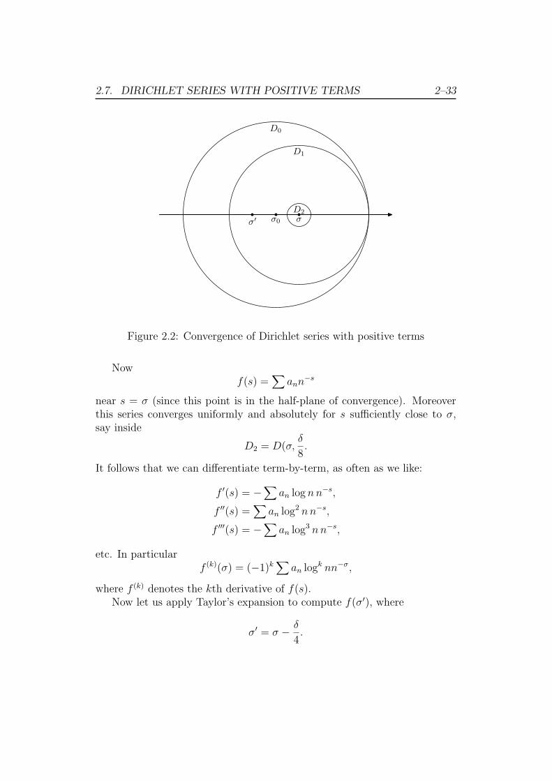
Figure 2.2: Convergence of Dirichlet series with positive terms
Nowf(s) =
∑ann
−s
near s = σ (since this point is in the half-plane of convergence). Moreoverthis series converges uniformly and absolutely for s sufficiently close to σ,say inside
D2 = D(σ,δ
8.
It follows that we can differentiate term-by-term, as often as we like:
f ′(s) = −∑
an log nn−s,
f ′′(s) =∑
an log2 nn−s,
f ′′′(s) = −∑
an log3 nn−s,
etc. In particularf (k)(σ) = (−1)k
∑an logk nn−σ,
where f (k) denotes the kth derivative of f(s).Now let us apply Taylor’s expansion to compute f(σ′), where
σ′ = σ − δ
4.
2.7. DIRICHLET SERIES WITH POSITIVE TERMS 2–34
We have
f(σ′) =∑k
1
k!f (k)(σ)(σ′ − σ)k
=∑k
(−1)k 1
k!f (k)(σ)
(δ
4
)k
.
Substituting from above for the f (k),
f(σ′) =∑k
1
k!
(δ
4
)k ∑n
an logk nn−σ.
Since all the terms on the right are positive (the two factors (−1)k cancellingout), the double series is absolutely convergent, and we can invert the orderof the summations:
f(σ′) =∑n
ann−σ∑k
1
k!logk n
(δ
4
)k
The series on the right may seem complicated, but common-sense tellsus what the sum must be. We could have carried out the whole operationentirely within the half-plane of convergence, in which case we know that
f(σ′) =∑
ann−σ′ .
Clearly this must still be true.In fact,
∑k
1
k!logk n
(δ
4
)k
=∑k
1
k!
(δ log n
4
)k
= eδ log n/4
= nδ/4
= nσ−σ′ ,
and so
f(σ′) =∑n
ann−σnσ−σ′
=∑n
ann−σ′ .
Thus f(σ′) converges, which is impossible since σ′ < σ0. We concludethat our original assumption is untenable: f(s) cannot be holomorphic in aneighbourhood of s = σ0. J
Chapter 3
The Prime Number Theorem
3.1 Statement of the theorem
The Prime Number Theorem asserts that
π(x) ∼ x
log x.
It is more convenient — and preferable — to express this in a slightly differentform.
Definition 3.1. For x ≥ e we set
Li(x) =∫ x
e
dt
log t.
Proposition 3.1. As x→∞,
Li(x) ∼ x
log x.
Proof I Integrating by parts,
Li(x) =∫ x
e
dt
log t
=
[t
1
log t
]x
e
+∫ x
et
1
t log2 tdt
=x
log x− e+
∫ x
e
dt
log2 t.
It is clear from this that
Li(x)→∞ as x→∞.
3–1
3.1. STATEMENT OF THE THEOREM 3–2
Thus the result will follow if we show that∫ x
e
dt
log2 t= o(Li(x)).
But ∫ x
e
dt
log2 t=∫ x1/2
e
dt
log2 t+∫ x
x1/2
dt
log2 t
≤ x1/2 +1
log(x1/2)
∫ x
x1/2
dt
log t
≤ x1/2 +2 Li(x)
log x.
From above,
Li(x) ≥ x
log x− e.
Thusx1/2 = o(Li(x));
and so ∫ x
e
dt
log2 t= o(Li(x)),
as required. J
Remark. We can extend this result to give an asymptotic expansion of Li(x).Integrating by parts,
∫ x
e
dt
logn t=
[t
1
logn t
]x
e
+∫ x
et
1
nt logn+1 tdt
=x
logn x− e+
1
n
∫ x
e
dt
logn+1 t.
It follows that
Li(x) =x
log x+
x
log2 x+
1
2!
x
log3 x+ · · ·+ 1
(n− 1)!
x
logn x+O(
x
logn+1 x).
Corollary 3.1. The Prime Number Theorem can be stated in the form:
π(x) ∼ Li(x).
3.2. PREVIEW OF THE PROOF 3–3
Remark. This is actually a more accurate form of the Prime Number Theo-rem, in the following sense. It has been shown that
π(x)− Li(x)
changes sign infinitely often, ie however large x gets we find that sometimesπ(x) ≥ Li(x), and sometimes π(x) < Li(x).
On the other hand, it follows from the Remark above that Li(x) is sub-stantially larger than x/ log x; and it has also been shown that π(x) > x/ log xfor all sufficiently large x.
3.2 Preview of the proof
The proof of the Prime Number Theorem is long and intricate, and dividedinto several more or less independent parts. A preview may therefore behelpful.
1. We start from Euler’s Product Formula
ζ(s) =∏
primes p
(1− p−s
)−1.
2. Logarithmic differentiation converts this to
−ζ′(s)
ζ(s)=∑p
log p p−s
1− p−s
=∑n
ann−s,
where
an =
log p if n = pr
0 otherwise.
3. The function ζ ′(s)/ζ(s) has poles wherever ζ(s) has a pole or zero. Itfollows from Euler’s Product Formula that ζ(s) has no zeros in <(s) >1. Accordingly ζ ′(s)/ζ(s) has a pole at s = 1 (with residue 1) and nopoles in <(s) > 1.
4. Although this is not essential, our argument is somewhat simplified ifwe ‘hive off’ the part of the Dirichlet series corresponding to higherprime-powers:
−ζ′(s)
ζ(s)=∑
log p p−s + h(s),
3.2. PREVIEW OF THE PROOF 3–4
whereh(s) =
∑log p
∑r>1
p−rs.
The function h(s) converges for <(s) > 1/2, as can be seen by com-parison with ζ(2s). Its partial sums are therefore of order o(n1/2+ε), byProposition 2.24. Consequently the contribution of h(s) can be ignoredin our argument.
5. We are left with the function
Θ(s) =∑p
log p p−s
=∫ ∞
0x−sdθ,
whereθ(x) =
∑p≤x
log p.
6. A (fairly) simple exercise in summation by parts shows that
π(x) ∼ x
log x⇐⇒ θ(x) ∼ x.
Accordingly, the proof of the Prime Number Theorem is reduced toshowing that
θ(x) ∼ x,
ie
θ(x) = x+ o(x).
7. The dominant term x in θ(x) arises from the pole of Θ(s) at s = 1, inthe following sense.
Consider the function ζ(s). This has a pole at s = 1 with residue 1,and it has partial sums
A(x) =∑n≤x
1 = [x] = x+O(1).
If now we subtract ζ(s) from Θ(s) then we ‘remove’ the pole at s = 1;and at the same time we subtract x from θ(x). More precisely, let
Ψ(s) = Θ(s)− ζ(s)=∑
ann−s,
3.2. PREVIEW OF THE PROOF 3–5
where
an =
log p− 1 if n = p,
−1 otherwise.
ThenΨ(s) =
∫ ∞
0x−sdψ,
whereψ(x) = θ(x)− [x] = θ(x)− x+O(1).
The Prime Number Theorem, as we have seen, is equivalent to thestatement that
ψ(x) = o(x).
8. Riemann hypothesised — we shall see why in Chapter 7 — that allthe zeros of ζ(s) in the ‘critical strip’ 0 ≤ <(s) ≤ 1 lie on the line<(s) = 1/2.
If that were so then Ψ(s) would be holomorphic in <(s) > 1/2, and itwould follow from Proposition 2.24 that
ψ(x) = o(x1/2+ε)
for any ε > 0, which is more than enough to prove the Theorem.
In fact, Riemann showed that with a little more care one can deducefrom his hypothesis that
ψ(x) = O(x1/2 log x),
ie
θ(x) = x+O(x1/2 log x),
from which it follows that
π(x) = Li(x) +O(x1/2 log x).
This — if it could be established — would constitute a remarkablystrong version of the Prime Number Theorem.
9. The Riemann Hypothesis would allow us to push back the abscissa ofconvergence of Ψ(s) all the way to σ = 1/2.
3.2. PREVIEW OF THE PROOF 3–6
It would be sufficient for our purposes if we could push it back to anyσ < 1, since this would imply that
ψ(x) = o(xσ+ε)
for any ε > 0.
Unfortunately, this has never been established. The best that we cando is to show that ζ(s) has no zeros actually on the line <(s) = 1:
ζ(1 + it) 6= 0
for t ∈ R \ {0}.This proof of this result is, in a sense, the heart of the proof of thePrime Number Theorem. The argument we use is rather strange; weshow that if ζ(s) had a zero at s = 1 + it then it would have a pole ats = 1 + 2it, which we know is not the case.
10. This takes us a tiny step forward; it shows that Ψ(s) is holomorphic in<(s) ≥ 1.
Proposition 2.24 only tells us that in this case
ψ(x) = o(x1+ε)
for any ε > 0, which is useless.
We need a much stronger result which tells us that if the Dirichlet series∑ann
−s is holomorphic everywhere on its critical line <(s) = σ0 (andsatisfies some natural auxiliary conditions) then its partial sums satisfy
A(x) = o(xσ0).
Results of this kind — relating partial sums of Dirichlet series to thebehaviour on the critical line — are known as Tauberian theorems,after Alfred Tauber, author of the first such result.
Tauber’s original result used real function theory, and was very diffi-cult. Fortunately, complex function theory yields a Tauberian theoremsufficient for our purpose with relative ease.
This allows us to conclude that
ψ(x) = o(x),
which as we have seen is tantamount to the Prime Number Theorem.
3.3. LOGARITHMIC DIFFERENTIATION 3–7
3.3 Logarithmic differentiation
Recall the notion of logarithmic differentiation. Suppose
f(x) = u1(x) · · ·un(x),
where ui(x) is differentiable and ui(x) > 0 for 1 ≤ i ≤ n. Taking logarithms,
log f(x) =∑
log ui(x).
Differentiating,f ′(x)
f(x)=∑ u′i(x)
ui(x).
it is easy to establish this result without using logarithms: on differentiatingthe product,
f ′(x) =∑
u1(x) · · ·u′i(x) · · ·un(x);
and the result follows on dividing by f(x). This shows that the result holdswithout assuming that ui(x) > 0. Indeed, by this argument the result holdsfor complex-valued functions: if
f(z) =∏
1≤i≤n
u(z),
where u1(z), . . . , un(z) are holomorphic in U , then
f ′(z)
f(z)=∑ u′i(z)
ui(z),
except where z = 0.We want to extend this to infinite products.
Proposition 3.2. Suppose an(z) (n ∈ N) is a sequence of holomorphic func-tions on the open set U ⊂ C; and suppose the series∑
|an(z)|
is uniformly convergent on U . Then
f(z) =∏n
(1 + an(z))
is holomorphic on U ; and
f ′(z)
f(z)=∑n
a′n(z)
1 + an(z)
on U .
3.4. FROM π(X) TO θ(X) 3–8
Proof I The partial products
Pn(z) =∏
m≤n
(1 + am(z))
converge uniformly to f(z) in U :
Pn(z)→ f(z).
It follows thatP ′
n(z)→ f ′(z).
HenceP ′
n(z)
Pn(z)→ f ′(z)
f(z).
ButP ′
n(z)
Pn(z)=∑m≤n
a′m(z)
1 + am(z).
We conclude that ∑n∈N
a′m(z)
1 + am(z)=f ′(z)
f(z).
J
3.4 From π(x) to θ(x)
Definition 3.2. We setθ(x) =
∑p≤x
log p.
Thus
θ(x) =
0 for x < 2
log 2 for 2 ≤ x < 3
log 6 for 3 ≤ x < 5
. . .
Proposition 3.3. π(x) ∼ Li(x) ⇐⇒ θ(x) ∼ x.
Proof I Suppose
π(x) ∼ Li(x) ∼ x
log x.
3.4. FROM π(X) TO θ(X) 3–9
Then
θ(X) =∑p≤x
log p
= log 2 +∫ X
elog x dπ
= log 2 + [log x π(x)]Xe −∫ X
e
1
xπ(x)dx
= log 2 + π(X) logX − 1−∫ X
e
π(x)
xdx.
Since π(x) ∼ x/ log x,
π(x) ≤ Cx
log x
for some constant C; and so
0 ≤∫ X
e
π(x)
xdx ≤ C
∫ X
e
dx
log x= C Li(x) = o(x),
by Proposition 3.1. Thus
π(x) ∼ x
log x=⇒ π(x) log x ∼ x =⇒ θ(x) ∼ x.
Conversely, supposeθ(x) ∼ x.
Then
π(X) = 1 +∫ X
e
1
log xdθ
= 1 +
[θ(x)
log x
]X
e
+∫ X
e
θ(x)
x log2 xdx
=θ(X)
logX+ (1− log 2) +
∫ X
e
θ(x)
x log xdx.
Nowθ(x) ∼ x =⇒ θ(x) ≤ Cx
for some C; and so
0 ≤∫ X
e
θ(x)
x log2 xdx
≤ C∫ X
e
dx
log2 x.
3.5. THE ZEROS OF ζ(S) 3–10
Henceθ(x)
log x≥ π(x) ≥ θ(x)
log x+ C
∫ X
e
dx
log2 x.
But
θ(x) ∼ x =⇒ θ(x)
log x∼ x
log x∼ Li(x),
while ∫ X
e
dx
log2 x= o(Li(x)),
as we saw in the proof of Proposition 3.1.We conclude that
π(x) ∼ x
log x∼ Li(x).
J
Corollary 3.2. The Prime Number Theorem is equivalent to:
θ(x) ∼ x.
3.5 The zeros of ζ(s)
Proposition 3.4. The Riemann zeta function ζ(s) has no zeros in the half-plane <(s) > 1.
Proof I This follows at once from Euler’s Product Formula:
ζ(s) =∏p
(1− p−s
)−1.
For the right-hand side converges absolutely for <(s) > 1; and by the defini-tion of convergence its value is 6= 0. J
We want to show that ζ(s) has no zeros on the line <(s) = 1. Thisis equivalent to showing that ζ ′(s)/ζ(s) has no poles on this line except ats = 1.
Proposition 3.5. For <(s) > 1,
ζ ′(z)
ζ(s)= −
∑ann
−s,
where
an =
log p if n = pr
0 otherwise.
3.5. THE ZEROS OF ζ(S) 3–11
Proof I The result follows at once on applying Proposition 3.2 to Euler’sProduct Formula, J
It is convenient to divide the Dirichlet series for ζ ′(s)/ζ(s) into two parts,the first corresponding to primes p, and the second to prime-powers pr(r ≥ 2).
Definition 3.3. We set
Θ(s) = −∑p
log p p−s.
Proposition 3.6. The function Θ(s) is holomorphic in <(s) > 1.
Proof I We know thatζ(s) =
∑n−s
is uniformly convergent in <(s) ≥ σ for any σ > 1. It follows that we candifferentiate term-by-term:
ζ ′(s) =∑
log nn−s
in <(s) > 1. Since the coefficients are all positive, the convergence is absolute.But the series for Θ(s) consists of some of the terms of ζ ′(s), and so alsoconverges absolutely in <(s) > 1. J
Proposition 3.7. For <(s) > 1,
ζ ′(z)
ζ(s)= −Θ(s) + h(s),
where h(s) is holomorphic in <(s) > 1/2.
Proof I We haveh(s) = −
∑p
log p∑r≥2
p−rs.
If σ = <(s) then |p−s| = p−σ. Thus∑p
log p∑r≥2
|p−rs| =∑p
log p∑r≥2
p−rσ
=∑p
log pp−2σ
1− p−σ
≤ 1
1− 2−σ
∑log p p−2σ
=1
1− 2−σΘ(2σ),
which converges for 2σ > 1, ie σ > 1/2, by Proposition 3.6. J
3.5. THE ZEROS OF ζ(S) 3–12
1 + 2it + σ
Figure 3.1: Comparing Θ(s) at three points
Proposition 3.8. The Riemann zeta function ζ(s) has no zeros on the line<(s) = 1:
ζ(1 + it) 6= 0 (t ∈ R \ {0}).
Proof I We shall show (in effect) that if ζ(s) has a zero at s = 1 + it thenit must have a pole at s = 1 + 2it; but we know that is impossible, since theonly pole of ζ(s) in <(s) > 0 is at s = 1.
We work with Θ(s) rather than ζ(s). If ζ(s) has a zero of multiplicity mat 1 + it then ζ ′(s)/ζ(s) has a simple pole with residue m, and so Θ(s) hasa simple pole with residue −m. Similarly, where ζ(s) has a pole of order M ,Θ(s) has a simple pole with residue M .
We are going to compare
Θ(1 + σ), Θ(1 + it+ σ), Θ(1 + 2it+ σ)
for small σ > 0 (Fig 3.1).We have
Θ(1 + σ) =∑
log p p−(1+σ),
Θ(1 + it+ σ) =∑
log p p−(1+σ)p−it,
Θ(1 + 2it+ σ) =∑
log p p−(1+σ)p−2it.
3.5. THE ZEROS OF ζ(S) 3–13
Note that
p−it = cos(t log p)− i sin(t log p),
p−2it = cos(2t log p)− i sin(2t log p).
Lemma 5. For all θ ∈ R,
cos 2θ + 4 cos θ + 3 ≥ 0.
Proof I For τ ∈ R,eiτ + e−iτ = 2 cos(τ) ∈ R.
Raising this to the fourth power,(eiτ + e−iτ
)4= e4iτ + e−4iτ + 4(e2iτ ) + e−2iτ ) + 6 ≥ 0,
ie
cos 4τ + cos 2τ + 3 ≥ 0.
The result follows on setting θ = 2τ . J
Lemma 6. For σ > 0,
< (Θ(1 + 2i+ σ) + 4Θ(1 + it+ σ) + 3Θ(1 + σ)) ≥ 0.
Proof I We have
<(p−2it + 4p−it + 3
)= cos(2t log p) + 4 cos(t log p) + 3 ≥ 0,
by the last Lemma.The result follows on multiplying by log p p−(1+σ) and summing. J
Remark. If we had taken squares instead of fourth powers, we would havefound
< (Θ(1 + it+ σ) + Θ(1 + σ)) ≥ 0,
which is not quite sufficient for our purposes.However, higher even powers would have done as well, eg sixth powers
yield
< (Θ(1 + 3it+ σ) + 6<(1 + 2it+ σ) + 15Θ(1 + it+ σ) + 10Θ(1 + σ)) ≥ 0,
which would have done.
3.5. THE ZEROS OF ζ(S) 3–14
Now suppose ζ(s) has a zero of multiplicity m at s = 1 + it, and supposeit also has a zero of multiplicity M at s = 1 + 2it, where we allow M = 0 ifthere is no zero. Then
Θ(1 + σ) =1
σ+ f1(σ),
Θ(1 + it+ σ) = −mσ
+ f2(σ),
Θ(1 + 2it+ σ) = −Mσ
+ f3(σ),
where f1(σ), f2(σ), f3(σ) are all continuous (and so bounded) for small σ.Adding, and taking the real part,
< (Θ(1 + 2i+ σ) + 4Θ(1 + it+ σ) + 3Θ(1 + σ)) =1− 4m− 3M
σ+ f(σ),
where f(σ) is continuous. By the last Lemma, this is ≥ 0 for all σ > 0. Itfollows that
1− 4m− 3M ≥ 0.
But that is impossible, since m,n ∈ N with m > 0. J
Remark. This proof is just a neat way of dressing up the following intuitiveargument.
We know that Θ(s) has a pole at s = 1, with residue 1:
Θ(1 + σ) =∑
log p p−(1+σ) =1
σ+O(σ).
Note that the terms are all positive.Now suppose ζ(s) has a zero of multiplicity m at s = 1 + it. Then Θ(s)
has a pole at s = 1 + it with residue −m:
Θ(1 + it+ σ) =∑
log p p−(1+σ) (cos(t log p) + i sin(t log p)) = −mσ
+O(σ).
Comparing this with the formula for Θ(1 + σ), and noting that
−1 ≤ cos(t log p) ≤ 1,
we see that in order to reach −1/σ (let alone −m/σ), cos(t log p) must beclose to −1 for almost all p.
Butcos τ = −1 =⇒ cos 2τ = +1.
3.6. THE TAUBERIAN THEOREM 3–15
Thus follows that cos(2t log p) is close to 1 for almost all p; and that in turnimplies that
Θ(1 + 2it+ σ) =∑
log p p−(1+σ (cos(2t log p) + i sin(2t log p))
is close to 1/σ, which means that Θ(s) must have a pole with residue 1 (ieζ(s) must have a simple pole) at s = 1 + 2it, which we know is not the case.
3.6 The Tauberian theorem
Proposition 3.9. Suppose the function f : [0,∞)→ C is
1. bounded; and
2. integrable over [0, X] for all X.
ThenF (s) =
∫ ∞
0e−xsf(x)dx
is defined and holomorphic in <(s) > 0.Suppose F (s) can be extended analytically to a holomorphic function in
<(s) ≥ 0. Then f(x) is integrable on [0,∞), and∫ ∞
0f(x)dx = F (0).
Proof I Suppose|f(x)| ≤ C.
For each X > 0,
FX(s) =∫ X
0e−xsf(x)dx.
is an entire function, ie holomorphic in the whole of the complex plane C.Suppose σ = <(s) > 0. If X < Y then
FY (s)− FX(s) =∫ Y
Xe−xsf(x)dx.
Thus
|FY (s)− FX(s)| ≤ C∫ Y
Xe−xσdx
=C
σ(e−Xσ − e−Y σ).
3.6. THE TAUBERIAN THEOREM 3–16
ThusFY (s)− FX(s)→ 0 as X, Y →∞.
HenceF (s) =
∫ ∞
0e−xsf(x)dx
converges for <(s) > 0.Moreover, our argument shows that this convergence is uniform in <(s) ≥
σ for each σ > 0. Hence F (s) is holomorphic in each such half-plane, and soin <(s) > 0.
We have to show that
FX(0) =∫ X
0f(x)dx→ F (0)
as X → ∞. (This will prove both that∫∞0 f(x)dx converges, and that its
value is F (0).)By Cauchy’s Theorem,
FX(0)− F (0) =1
2πi
∫γ(FX(s)− F (s))
ds
s
around any contour γ surrounding 0 within which F (s) is holomorphic. Wecan even introduce a holomorphic factor λ(s) satisfying λ(0) = 1:
FX(0)− F (0) =1
2πi
∫γ(FX(s)− F (s))λ(s)
ds
s.
We choose the contour γ in the following way. Suppose R > 0. (We shalllater let R → ∞.) By hypothesis, F (s) is holomorphic at each point s = itof the imaginary axis, ie it is holomorphic in some circle centred on s = it. Itfollows by a standard compactness argument that we can find a δ = δ(R) > 0such that F (s) is holomorphic in the rectangle
{s = x+ iy : −δ ≤ x ≤ 0;−R ≤ y ≤ R}.
To simplify the later computations we assume — as we evidently may —that δ ≤ R.
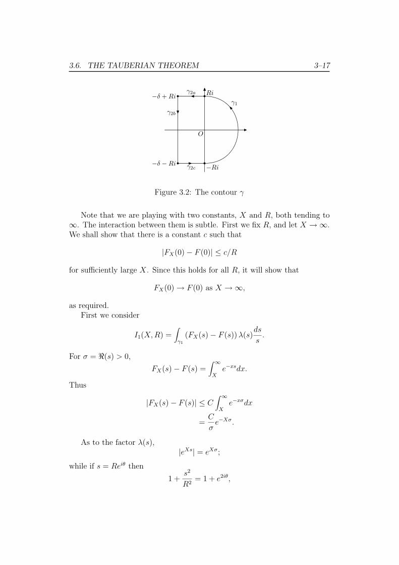
We take γ to be the contour formed by a large semicircle γ1 of radius Rin the positive half-plane, completed by 3 sides γ2 = γ2a + γ2b + γ2c of theabove rectangle in the negative half-plane (Fig 3.2).
We also choose our factor λ(s) (for reasons that will become apparent)to be
λ(s) = eXs
(1 +
s2
R2
).
3.6. THE TAUBERIAN THEOREM 3–17
O
Ri
−Ri
−δ + Ri
−δ −Ri
γ1
γ2a
γ2b
γ2c
Figure 3.2: The contour γ
Note that we are playing with two constants, X and R, both tending to∞. The interaction between them is subtle. First we fix R, and let X →∞.We shall show that there is a constant c such that
|FX(0)− F (0)| ≤ c/R
for sufficiently large X. Since this holds for all R, it will show that
FX(0)→ F (0) as X →∞,
as required.First we consider
I1(X,R) =∫
γ1
(FX(s)− F (s))λ(s)ds
s.
For σ = <(s) > 0,
FX(s)− F (s) =∫ ∞
Xe−xsdx.
Thus
|FX(s)− F (s)| ≤ C∫ ∞
Xe−xσdx
=C
σe−Xσ.
As to the factor λ(s),|eXs| = eXσ;
while if s = Reiθ then
1 +s2
R2= 1 + e2iθ,
3.6. THE TAUBERIAN THEOREM 3–18
and so
|1 +s2
R2| = eiθ + e−iθ = 2 cos θ =
2σ
R.
Hence
|(FX(s)− F (s))λ(s)| ≤ C
σe−Xσ · eXσ 2σ
R
=2C
R.
(We see now how the two parts of λ(s) were chosen to cancel out thefactors e−Xσ and 1/σ.)
Since s = Reiθ,ds
s= ieiθdθ;
and so
|I1(X,R)| ≤ 2Cπ
R.
Turning to the part γ2 of the integral in the negative half-plane, we con-sider FX(s) and F (s) separately:
I2(X,R) = I ′2(X,R) + I ′′2 (X,R),
where
I ′2(X,R) =∫
γ2
FX(s)λ(s)ds
s
I ′′2 (X,R) =∫
γ2
F (s)λ(s)ds
s.
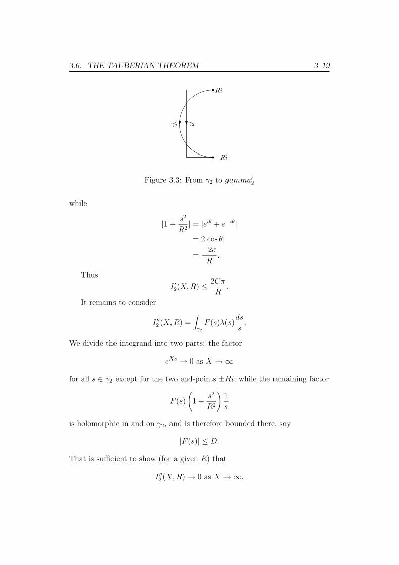
Since FX(s) is an entire function, we can replace the contour γ2 in theintegral I ′2(X,R) by the half-circle γ′2 of radius R in the negative half-plane(Fig 3.3), ie the complementary half-circle to γ1.
We have
FX(s) =∫ X
0e−xsf(x)dx.
Thus if σ = <(s) ≤ 0 then
|FX(s)| ≤ C∫ X
0e−xσdx
≤ C
−σe−Xσ.
As before,|eXs| = eXσ;
3.6. THE TAUBERIAN THEOREM 3–19
Ri
−Ri
γ′2
γ2
Figure 3.3: From γ2 to gamma′2
while
|1 +s2
R2| = |eiθ + e−iθ|
= 2|cos θ|
=−2σ
R.
Thus
I ′2(X,R) ≤ 2Cπ
R.
It remains to consider
I ′′2 (X,R) =∫
γ2
F (s)λ(s)ds
s.
We divide the integrand into two parts: the factor
eXs → 0 as X →∞
for all s ∈ γ2 except for the two end-points ±Ri; while the remaining factor
F (s)
(1 +
s2
R2
)1
s
is holomorphic in and on γ2, and is therefore bounded there, say
|F (s)| ≤ D.
That is sufficient to show (for a given R) that
I ′′2 (X,R)→ 0 as X →∞.
3.7. PROOF 3–20
More precisely,
|I2a(X,R)|, |I2c(X,R)| ≤ D∫ δ
0e−Xσdσ
≤ D
X,
while|I2b(X,R)| ≤ 2Re−Xδ.
Thus all three parts of I2(X,R) tend to 0, and so
I2(X,R)→ 0 as X →∞
for each R > 0.Putting all this together, we deduce that
|FX(0)− F (0)| ≤ 5Cπ
R
for sufficiently large X. It follows that
FX(0)− F (0)→ 0 as X →∞,
as required. J
3.7 Proof
We now have all the ingredients to complete the proof of the Prime NumberTheorem.
Proof I By Proposition 3.3, it is sufficient to prove that
θ(x) ∼ x.
We need to ‘bootstrap’ this result, by showing first that
θ(x) = O(x).
Lemma 7. There exists a constant C such that
θ(x) ≤ Cx
for all x ≥ 0.
3.7. PROOF 3–21
Proof I Consider the binary coefficient(2n
n
)=
(2n)(2n− 1) · · · (n+ 1)
1 · 2 · · ·n.
This is of course an integer; and all the primes between n and 2n are factors,since each divides the top but not the bottom. Thus
∏n<p≤2n
p ≤(
2n
n
).
But (2n
n
)≤ 22n,
since the binomial coefficient is one term in the expansion of (1 + 1)2n. Thus∏n<p≤2n
p ≤ 22n.
Taking logarithms of both sides,
θ(2n)− θ(n) ≤ 2n log 2.
Setting n = 2m−1, 2m−2, . . . , successively,
θ(2m)− θ(2m−1) ≤ 2m log 2,
θ(2m−1)− θ(2m−2) ≤ 2m−1 log 2,
. . .
θ(2)− θ(1) ≤ 2 log 2.
Adding,
θ(2m) = θ(2m)− θ(1) ≤ (2m + 2m−1 + · · ·+ 2) log 2
≤ 2m+1 log 2.
Now suppose2m−1 < x ≤ 2m.
Then
θ(x) ≤ θ(2m)
≤ 2m+1 log 2
= (4 log 2)2m−1
≤ (4 log 2)x.
J
3.7. PROOF 3–22
Now letψ(x) = θ(x)− x.
We have to show thatψ(x) = o(x).
For <(s) > 1, let
Ψ(s) =∫ ∞
1x−sdψ.
Integrating by parts,∫ X
1x−sdψ =
[x−sψ(x)
]X1
+ s∫ X
1x−sψ(x)
dx
x
= X−sψ(X)− 1 + s∫ X
1x−sψ(x)
dx
x.
ButX−sψ(X)→ 0 as X →∞
since|ψ(X)| ≤ max(θ(X), X) ≤ C ′X.
Thus
Ψ(x) = 1 + s∫ ∞
1x−sψ(x)
dx
x
= 1 + s∫ ∞
1x−s(θ(x)− x)dx
x
= 1 + s(Θ(s)− 1
s− 1
).
Now Θ(s) has a pole at s = 1 with residue 1 (arising from the pole ofζ(s)). It follows that Ψ(s) is holomorphic at s = 1; and it has no poleselsewhere on <(s) = 1, since Θ(s) does not. Thus
1
s(Ψ(s)− 1) =
∫ ∞
1x−sψ(x)
dx
x
is holomorphic in <(s) ≥ 1,On making the change of variable x = et (we can think of this as passing
from the multiplicative group R+ to the additive group R),
1
s(Ψ(s)− 1) =
∫ ∞
1x−sψ(x)
dx
x
=∫ ∞
0e−tsψ(et)dt.
3.7. PROOF 3–23
We are almost in a position to apply our Tauberian theorem. There is onelast change; the theorem, as we expressed it, assumed that the critical linewas the imaginary axis <(s) = 0. But the critical line of Ψ(s) is <(s) = 1.We therefore set
s = 1 + s′.
We have
1
sΨ(s) =
∫ ∞
0e−t(1+s′)ψ(et)dt
=∫ ∞
0e−ts′e−tψ(et)dt.
Now we can apply the theorem, since
|e−tψ(et)| ≤ |e−tθ(et|≤ e−tCet
≤ C,
ie e−tψ(et) is bounded; while
1
1 + s′Ψ(1 + s′)
is holomorphic on <(s′) = 0.We conclude that ∫ ∞
0e−tψ(et)dt
converges to Ψ(1). (We only need the convergence, not the value.)Changing variables back to x = et, we deduce that∫ ∞
1
ψ(x)
x2dx =
∫ ∞
1
θ(x)− xx2
dx
converges.It remains to show that this implies that
θ(x) ∼ x.
Suppose that were not so. Then either
lim sup θ(x)
x> 1
or elselim inf θ(x)
x< 1
3.7. PROOF 3–24
(or both). In other words, there exists a δ > 0 such that either
θ(X) ≥ (1 + δ)X
for arbitrarily large X, or else
θ(X) ≤ (1− δ)X
for arbitrarily large X.Suppose
θ(X) ≥ (1 + δ)X.
Since θ(x) is increasing, it follows that
X ≤ x ≤ (1 + δ)X =⇒ θ(x) ≥ θ(X) ≥ (1 + δ)X ≥ x,
ie
θ(x)− x ≥ 0
on the interval [X, (1 + δ)X].More precisely,∫ (1+δ)X
X
θ(x)− xx2
dx ≥∫ (1+δ)X
X
(1 + δ)X − xx2
dx
≥∫ 1+δ
1
(1 + δ)− yy2
dy, on setting x = Xy,
≥ 1
(1 + δ)2
∫ 1+δ
1(1 + δ − y)dy
≥ 1
(1 + δ)2
∫ δ
0u du
=δ2
2(1 + δ)2.
But the fact that there exist such intervals [X, (1 + δ)X] with arbitrarilylarge X contradicts the convergence of∫ ∞ θ(x)− x
x2dx,
which we have already established. We conclude that
lim supθ(x)
x≤ 1.
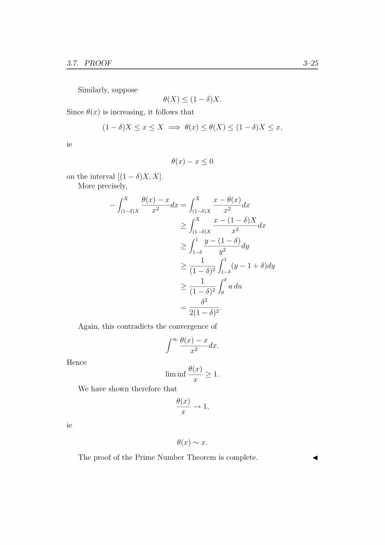
3.7. PROOF 3–25
Similarly, supposeθ(X) ≤ (1− δ)X.
Since θ(x) is increasing, it follows that
(1− δ)X ≤ x ≤ X =⇒ θ(x) ≤ θ(X) ≤ (1− δ)X ≤ x,
ie
θ(x)− x ≤ 0
on the interval [(1− δ)X,X].More precisely,
−∫ X
(1−δ)X
θ(x)− xx2
dx =∫ X
(1−δ)X
x− θ(x)x2
dx
≥∫ X
(1−δ)X
x− (1− δ)Xx2
dx
≥∫ 1
1−δ
y − (1− δ)y2
dy
≥ 1
(1− δ)2
∫ 1
1−δ(y − 1 + δ)dy
≥ 1
(1− δ)2
∫ δ
0u du
=δ2
2(1− δ)2.
Again, this contradicts the convergence of∫ ∞ θ(x)− xx2
dx.
Hence
lim infθ(x)
x≥ 1.
We have shown therefore that
θ(x)
x→ 1,
ie
θ(x) ∼ x.
The proof of the Prime Number Theorem is complete. J
Chapter 4
The Dirichlet L-functions
4.1 Characters of a finite abelian group
4.1.1 Definition of a character
Definition 4.1. A character of a finite abelian group A is a homomorphism
χ : A→ C×.
The character defined by the trivial homomorphism is called the principalcharacter and is denoted by χ1:
χ1(a) = 1
for all a ∈ A.
Remarks. 1. We generally denote abelian groups multiplicatively — con-trary perhaps to the usual practice — because the groups (Z/m)× towhich we shall apply the theory are multiplicative.
2. For a map χ : A→ C× to be a character it is sufficient that
χ(ab) = χ(a)χ(b)
for all a, b ∈ A. For if that is so then
e2 = e =⇒ χ(e)2 = χ(e) =⇒ χ(e) = 1;
and furthermore, if a ∈ A then an = e for some n by Lagrange’sTheorem, so that
a−1 = an−1,
4–1
4.1. CHARACTERS OF A FINITE ABELIAN GROUP 4–2
and therefore
χ(a−1) = χ(an−1) = χ(a)n−1 = χ(a)−1,
sinceχ(a)n = χ(an) = χ(e) = 1.
Example. Suppose
A = Cn = {e, g, g2, . . . , gn−1 : gn = e}.
Let ω = e2πi/n.The cyclic group Cn has just n characters, namely
χ(j) : gi → ωij (0 ≤ j < n).
For these are certainly characters of Cn; while conversely, if χ is such acharacter then
gn+1 = g =⇒ χ(g)n+1 = χ(gn+1) = χ(g)
=⇒ χ(g) = ωj for some j ∈ [0, n− 1]
=⇒ χ = χ(j).
Proposition 4.1. If χ is a character of the finite abelian group A then
|χ(a)| = 1
for all a ∈ A.
Proof I By Lagrange’s Theorem, an = e for some n. Hence
χ(a)n = χ(an) = χ(e) = 1 =⇒ |χ(a)| = 1.
J
Proposition 4.2. For any character χ of A,
χ(a−1) = χ(a).
Proof I This follows at once from Proposition 4.1, since
|z| = 1 =⇒ z−1 = z.
J
4.1. CHARACTERS OF A FINITE ABELIAN GROUP 4–3
4.1.2 The dual group A∗
Proposition 4.3. The characters of a finite abelian group A form a groupA∗ under multiplication:
(χχ′)(a) = χ(a)χ′(a).
The principal character χ1 is the identity of A∗; and the inverse of χ is thecharacter
χ−1(a) = χ(a−1) = χa.
Proof I The first part follows at once, since
(χχ′)(ab) = χ(ab)χ′(ab)
= (χ(a)χ(b))(χ′(a)χ′(b))
= (χ(a)χ′(a))(χ(b)χ′(b))
= (χχ′)(a)(χχ′)(b)
The last two parts are trivial. J
Definition 4.2. The group A∗ of characters is called the dual group of A.
Example. If A = Cn then, as we have seen,
A∗ = {χ(0), χ(1), . . . , χ(n−1)},
where χ(j)(gi) = ωij. It is easy to see that
χ(i)χ(i′) = χ(i+i′ mod n).
It follows that the characters can be identified with the group Z mod m;hence
C∗n∼= Z/(n) ∼= Cn.
We may say that the cyclic group Cn is self-dual.
Proposition 4.4. Every finite abelian group A is self-dual, ie
A∗ ∼= A.
Proof I We know that A is expressible as a product of cyclic groups:
A = Cn1 × · · · × Cnr .
Lemma 8. If A = B × C then
A∗ = B∗ × C∗.
4.1. CHARACTERS OF A FINITE ABELIAN GROUP 4–4
Proof I We can identify B,C with the subgroups B × {e}, {e} × C of A.Thus each character χ of A defines characters χB, χC of B,C by restriction.Moreover, since
(b, c) = (b, e) · (e, c)it follows that
χ(b, c) = χB(b)χC(c).
This gives a one-one correspondence
χ←→ (χB, χC)
between characters of A, and pairs of characters of B and C; and it is straight-forward to verify that this is an isomorphism. J
It follows from the Lemma that
A∗ = C∗n1× · · · × C∗
nr.
But we have seen thatC∗
n∼= Cn
for any cyclic group Cn. It follows that
A∗ ∼= A.
J
Remark. This isomorphism is non-canonical, in the sense that there is nonatural way of picking out one such isomorphism.
More precisely, the functor
A A∗
is contravariant, ie each homomorphism
α : A→ B
gives rise to a homomorphism
α∗ : B∗ → A∗
in the opposite direction; and there is no way in general of choosing anisomorphism θ : A→ A∗ such that the diagram
Aθ−−−→ A∗yα
xα∗
Aθ−−−→ A∗
is commutative for all α.
4.1. CHARACTERS OF A FINITE ABELIAN GROUP 4–5
If a ∈ A then the mapχ 7→ χ(a)
defines a character of the group A∗. This gives a (natural) homomorphism
A→ A∗∗.
Proposition 4.5. For any finite abelian group
A∗∗ = A.
Proof I Since|A∗∗| = |A∗| = |A|,
it is sufficient (by the Pigeon-Hole Principle) to show that the map
A→ A∗∗
is injective.
Lemma 9. If a 6= e then there exists a character χ such that
χ(a) 6= 1.
Proof I The elements
B = {b : χ(b) = 1 for all χ ∈ A∗}
form a subgroup B ⊂ A; and every character of A is a character of thequotient-group A/B, ie
A∗ = (A/B)∗.
But that is impossible unless B = {e}, since otherwise
|(A/B)∗| = |A/B| < |A| = |A∗|.
J
We conclude that the homomorphism
A→ A∗∗
is injective, and is therefore an isomorphism. J
4.1. CHARACTERS OF A FINITE ABELIAN GROUP 4–6
Remark. The character theory of finite abelian groups is a more-or-less trivialcase of the character theory of locally compact abelian groups.
Each such group A has a dual A∗, consisting of the characters, ie continu-ous homomorphisms χ : A→ C× such that |χ(a)| = 1 for all a. (For compactabelian groups this last condition necessarily holds. But in the non-compactcase we must impose it.)
For example, the additive group R is self-dual: R∗ = R. This is the basisof the Fourier integral.
The dual of the torus T is the additive group of integers: T∗ = Z. Thatis the basis of Fourier series.
The character theory of general locally compact abelian groups is some-times called generalised Fourier analysis.
4.1.3 Sums over elements
Proposition 4.6. Suppose χ is a character of the finite abelian group A.Then ∑
a∈A
χ(a) =
|A| if χ = χ1,
0 otherwise.
Proof I If χ = χ1, ie χ(a) = 1 for all a ∈ A then the sum is clearly |A|.Suppose χ 6= χ1. Then we can find a b ∈ A such that
χ(b) 6= 1.
As a runs over A so does ab. Hence∑a∈A
χ(a) =∑a∈A
χ(ab)
= χ(b)∑a∈A
χ(a).
Thus
(χ(b)− 1)∑a
χ(a) = 0,
and so
∑a
χ(a) = 0.
J
4.1. CHARACTERS OF A FINITE ABELIAN GROUP 4–7
Proposition 4.7. Suppose χ, χ′ are characters of the finite abelian group A.Then ∑
a∈A
χ(a)χ′(a) =
|A| if χ = χ′,
0 otherwise.
Proof I By Proposition 4.3,
χ(a)χ′(a) = χ−1(a)χ′(a)
= (χ−1χ′)(a).
Hence ∑a∈A
χ(a)χ′(a) =∑a∈A
(χ−1χ′)(a),
and the result follows from Proposition 4.6, since
χ−1χ′ = χ1 ⇐⇒ χ = χ′.
J
4.1.4 Sums over characters
Proposition 4.8. Suppose a ∈ A, where A is a finite abelian group. Then
∑χ∈A∗
χ(a) =
|A| if a = e,
0 otherwise.
Proof I If a = e then χ(a) = 1 for all χ ∈ A∗ and the sum is evidently |A|.Suppose a 6= e. By the Lemma to Proposition 4.5, we can find a χ′ ∈ A∗
such thatχ′(a) 6= 1.
As χ runs over A∗ so does χ′χ. Hence∑χ∈A∗
χ(a) =∑
χ∈A∗(χ′χ)(a)
= χ′(a)∑
χ∈Aast
χ(a).
Thus
(χ′(a)− 1)∑χ
χ(a) = 0,
and so ∑χ
χ(a) = 0.
J
4.1. CHARACTERS OF A FINITE ABELIAN GROUP 4–8
Proposition 4.9. Suppose ab ∈ A, where A is a finite abelian group. Then
∑χ∈A∗
χ(a)χ(b) =
|A| if a = b,
0 otherwise.
Proof I Since
χ(a)χ(b) = χ(a−1)χ(a)
= χ(a−1b).
the result follows at once from Proposition 4.8. J
Remark. Alternatively, Propositions 4.8 and 4.9 follow at once from Propo-sitions 4.6 and 4.7, on applying the latter to the dual group A∗, and usingthe fact that A∗∗ = A.
4.1.5 Functions on a finite abelian group
Suppose A is a finite abelian group. The functions
f : A→ C
form a vector space C(A) (over C) of dimension |A|, of which the |A| char-acters of A are elements.
It is convenient to introduce an inner product in the space C(A) of func-tions on A.
Definition 4.3. If f(a), g(a) ∈ C(A) we set
〈f g〉 =1
|A|∑a∈A
f(a)g(a).
It is a straightforward matter to verify that this is a positive-definitehermitian form, ie
1. 〈g f〉 = 〈f g〉;
2. 〈f f〉 ≥ 0, and 〈f f〉 = 0 ⇐⇒ f = 0;
3. 〈f λ1g1 + λ2g2〉 = λ1 〈f g1〉+ λ2 〈f g2〉.
Now we can re-state Proposition 4.7 as follows.
4.1. CHARACTERS OF A FINITE ABELIAN GROUP 4–9
Proposition 4.10. The characters of A form an orthonormal set:
〈χ′ χ〉 =
1 if χ = χ′,
0 otherwise.
Corollary 4.1. The characters are linearly independent.
Proof I Suppose ∑i
λiχi = 0.
Then
0 =
⟨χj
∑i
λiχi
⟩=∑
i
λi 〈χj χi〉
= λj
for all j. J
Corollary 4.2. The characters form a basis for C(A). Explicitly, each func-tion f : A→ C is uniquely expressible as a linear combination of characters:
f =∑χ
λχχ,
with
λχ = 〈χ f〉 =1
|A|∑a∈A
χ(a)f(a).
Proof I The characters must form a basis for C(A), since they are linearlyindependent and there are
|A| = dimC(A)
of them.So certainly
f =∑χ
λχχ,
for some λχ ∈ C. To determine these coefficients, we take the inner-productwith χ′:
〈χ′ f〉 =∑〈χ′ λχχ〉
= λχ′ .
J
4.2. MULTIPLICATIVE CHARACTERS MODM 4–10
We shall make use of one particular case of this.
Corollary 4.3. Let cb(x) denote the characterestic function of the elementb, ie
cb(a) =
1 if a = b,
0 otherwise.
Then 〈cb χ〉 = χ(b)/|A|, and so
cb =1
|A|∑
χ∈A∗χ(b)χ.
4.2 Multiplicative characters modm
Suppose m ∈ N, m 6= 0. We denote the ring of residue classes modmby Z/(m). We can identify the classes in Z/(m) with their representativesr, 0 ≤ r < m.
Recall that we denote by φ(m) the number of residue classes coprime tom, ie
φ(m) = ‖{r : 0 ≤ r < m, gcd(r,m) = 1}‖.
Proposition 4.11. The φ(m) residue classes coprime to m form a multi-plicative group.
Proof I If r, s are coprime to m then so is rs. It remains to show that eachsuch residue class has an inverse s mod m:
rs ≡ 1 mod m.
If gcd(r,m) = 1 then the map
x 7→ rx mod m : Z/(m)→ Z/(m)
is injective, since
rx ≡ ry mod m =⇒ m | r(x− y) =⇒ m | (x− y) =⇒ x ≡ y mod m.
It follows (by the Pigeon-Hole Principle) that this map is surjective. Inparticular there exists an s such that
rs ≡ 1 mod 1.
J
4.2. MULTIPLICATIVE CHARACTERS MODM 4–11
Definition 4.4. We denote this multiplicative group by Z/m)×.
Example.
(Z/1)× = {1},(Z/2)× = {1},(Z/3)× = {1, 2} = {±1} ∼= C2,
(Z/4)× = {1, 3} = {±1} ∼= C2,
(Z/5)× = {1, 2, 3, 4} = {±1,±2} ∼= C4,
(Z/6)× = {1, 5} = {±1} ∼= C2,
(Z/7)× = {1, 2, 3, 4, 5, 6} = {±1,±2,±3} ∼= C6,
(Z/8)× = {1, 3, 5, 7} = {±1,±3} ∼= C2 × C2,
(Z/9)× = {1, 2, 4, 5, 7, 8} = {±1,±2,±4} ∼= C6,
Proposition 4.12. Suppose m = m1m2, where gcd(m1,m2) = 1. Then
(Z/m)× = (Z/m1)× × (Z/m2)
×.
Proof I By the Chinese Remainder Theorem, the ring-homomorphism
Θ : Z/(m)→ Z/(m1)× Z/(m2) : x 7→ (x mod m1, x mod m2)
is an isomorphism.Suppose r ∈ Z/(m). Then
gcd(r,m) = 1 ⇐⇒ gcd(r,m1) = 1 = gcd(r,m2).
Hence Θ maps (Z/m)× onto (Z/m1)××(Z/m2)
×, which proves the result. J
Example. Since gcd(4, 3) = 1,
(Z/12)× = (Z/4)× × (Z/3)×,
with the pairings
1 7→ (1, 1),
5 7→ (1, 2),
7 7→ (3, 1),
11 7→ (3, 2).
4.2. MULTIPLICATIVE CHARACTERS MODM 4–12
Corollary 4.4. If gcd(m,n) = 1 then
φ(mn) = φ(m)φ(n).
Corollary 4.5. Supposem = pe1
1 · · · perr ,
where p1, . . . , pr are distinct primes. Then
(Z/m)× = (Z/pe11 )× · · · × (Z/per
r )×.
Thus the structure of the groups (Z/m)× is reduced to the structure ofthe groups Z/pr)×. Although we shall not make use of the following results,it may be helpful to know what these groups look like.
Proposition 4.13. If p is prime then the group (Z/p)× is cyclic.
Proof I We have(Z/p)× = {1, 2, . . . , p− 1}.
Since each element of the ring Z/(p) except 0 is invertible, Z/(p) is in fact afield.
By Lagrange’s Theorem, if G is a group of order n then
gn = e
for all g ∈ G. The smallest number e > 0 such that
ge = e
is called the exponent of G. By Lagrange’s Theorem, e | n.
Lemma 10. The exponent of (Z/p)× is p− 1.
Proof I Each element r ∈ (Z/p)∗ satisfies the equation
xe − 1 = 0
over the field Z/(p). But this equation has at most e roots. It follows that
p− 1 ≤ e.
Since e | (p− 1) it follows that
e = p− 1.
J
4.2. MULTIPLICATIVE CHARACTERS MODM 4–13
Lemma 11. Suppose A is a finite abelian group of exponent e. Then A hasan element of order e.
Proof I Lete = pe1
1 · · · perr .
For each i there must be an element ai whose order is divisible by peii ; for
otherwise pi would occur to a lower power in the exponent e. Let
order(ai) = peii qi.
Thenbi = aqi
i
has order ei.But if A is a finite abelian group, and a, b ∈ A have orders r, s then
gcd(r, s) = 1 =⇒ order(ab) = rs.
For suppose order(ab) = n. Then
(ab)rs = 1 =⇒ n | rs.
On the other hand, since r, s are coprime we can find x, y ∈ Z such that
rx+ sy = 1.
But then(ab)sy = asy = a1−rx = a.
It follows that r | n. Similarly s | n. Since gcd(r, s) = 1 this implies that
rs | n.
Hencen = rs.
Applying this toa = b1 · · · br
we conclude that a has order
pe11 · · · per
r = e.
J
By these two Lemmas, we can find an element a ∈ (Z/p)× of order p− 1.Hence (Z/p)× is cyclic. J
4.2. MULTIPLICATIVE CHARACTERS MODM 4–14
Generators of (Z/p)× are called primitive roots modp.If a is a primitive root modp then it is easy to see that ar is a primitive
root if and only if gcd(r, p−1) = 1. It follows that there are φ(p−1) primitiveroots modp.
For example, there are just φ(6) = 2 primitive roots mod 7, namely 3 and5 = 3−1 mod 7.
Proposition 4.14. If p is an odd prime number then the multiplicative group
(Z/pe)×
is cyclic for all e ≥ 1.
Proof I We have proved the result for e = 1. We derive the result for e > 1in the following way.
The group (Z/pe)× has order
φ(pe) = pe−1(p− 1).
By the last Proposition, there exists an element a with
order(a mod p) = p− 1.
Evidentlyorder(a mod p) | order(a mod pe).
Thus the order of a mod p is divisible by p − 1. It is therefore sufficient byLemma 11 to show that there exists an element of order pe−1 in the group.
The elements of the form x = 1 + py form a subgroup
S = {x ∈ (Z/pe)× : x ≡ 1 mod pe}
of order pe−1. It suffices therefore to show that this subgroup is cyclic.That is relatively straightforward, since this group is ‘almost additive’.
Each element of the group has order pj for some j. We have to show thatsome element x = 1 + py has order pe−1, ie
(1 + py)pe−2 6≡ 1 mod pe.
By the binomial theorem,
(1 + py)pe−2
= 1 + pe−2py +
(pe−2
2
)p2y2 +
(pe−2
3
)p3y3 + · · · .
4.2. MULTIPLICATIVE CHARACTERS MODM 4–15
We claim that all the terms after the first two are divisible by pe, ie
pe |(pe−2
r
)pryr
for r ≥ 2. To see this, note that(pe−2
r
)pr =
pe−2(pe−2 − 1) · · · (pe−2 − r + 1)
1 · 2 · · · rpr
=(pe−2 − 1) · · · (pe−2 − r + 1)
1 · 2 · · · (r − 1)pe−2p
r
r
=
(pe−2 − 1
r − 1
)pe−2p
r
r.
Thus it is sufficient to show that
p2 | pr
r
for r ≥ 2; and that follows at once from the fact that
pr−1 > r,
eg becausepr−1 > (1 + 1)r−1 ≥ 1 + (r − 1) = r.
Thus any element of the form 1 + py where y is not divisible by p (forexample, 1 + p) must have multiplicative order pe−1, and so must generateS. In particular the subgroup S is cyclic, and so (Z/pe)× is cyclic. J
Turning to p = 2, it is evident that (Z/2)× is trivial, while (Z/4)× = C2.
Proposition 4.15. If e ≥ 3 then
(Z/2e)× ∼= C2 × C2e−2 .
Proof I Sinceφ(2e) = 2e−1,
(Z/2e)× contains 2e−1 elements. By the Structure Theorem for finite abeliangroups, it is sufficient to show that (Z/2e)× has exponent 2e−2. For then oneof the factors in
(Z/2e)× = C2e1 × · · · × C2er
must be C2e−2 , and the remaining factor must be C2.
4.2. MULTIPLICATIVE CHARACTERS MODM 4–16
This is certainly true for (Z/8)× = {±1,±3}, since
(±1)2 = (±3)2 = 1.
It follows that (Z/2e)× cannot be cyclic for e > 3; for if a generated(Z/2e)× then it would generate Z/8)×. (In effect, (Z/8)× is a quotient groupof (Z/2e)×.) Thus the Proposition will be proved if we can find an elementof order 2e−2 mod 2e.
We argue as we did for odd p, except that now we take x = 1 + 22y. Bythe binomial theorem,
(1 + 22y)2e−3
= 1 + 2e−322y +
(2e−3
2
)24y2 +
(2e−3
3
)26y3 + · · · .
As before, all the terms after the first two are divisible by 2e, ie
2e |(pe−3
r
)22ryr
for r ≥ 2. For(2e−3
r
)22r =
2e−3(2e−3 − 1) · · · (2e−3 − r + 1)
1 · 2 · · · r22r
=(2e−3 − 1) · · · (2e−3 − r + 1)
1 · 2 · · · (r − 1)2e−3 22r
r
=
(2e−3 − 1
r − 1
)2e−3 22r
r.
Thus it is sufficient to show that
23 | 22r
r
for r ≥ 2; and that follows at once from the fact that
22(r−1) > r,
eg because
22(r−1) = (1 + 1)2(r−1) ≥ 1 + 2(r − 1) + 1 = 2r.
Thus any element of the form 1 + 22y with y odd (for example, 5) musthave multiplicative order 2e−1, which as we have seen is sufficient to provethe result. J
4.2. MULTIPLICATIVE CHARACTERS MODM 4–17
4.2.1 Characters and multiplicative functions
Suppose χ is a character of (Z/m)×. Thus in principle χ is a function
χ : (Z/m)∗ → C×.
However, we extend χ to a function
χ : Z/(m)→ C,
by settingχ(r) = 0 if gcd(r,m) > 1.
Now we extend χ to a function
χ : N→ Z/(m)→ C
by composition. (It should cause no confusion that we use the same symbolχ for all three functions.)
For example, suppose m = 6. Since φ(6) = 2, there are just 2 multiplica-tive characters mod6, the principal character χ1 and the character
χ(r) =
1 if r ≡ 1 mod 6,
−1 if r ≡ 5 mod 6.
The corresponding function χ : N→ C is given by
χ(n) =
0 if n ≡ 0, 2, 3, 4 mod 6,
1 if n ≡ 1 mod 6,
−1 if n ≡ 5 mod 6.
Recall that a functionχ : N→ C
is said to be multiplicative if
gcd(m,n) = 1 =⇒ χ(mn) = χ(m)χ(n),
and χ(0) = 0, χ(1) = 1. (We include the latter condition to exclude the casewhere f(n) = 0 for all n).
We say that χ(n) is strictly multiplicative if
χ(mn) = χ(m)χ(n)
for all m,n ∈ N, and χ(0) = 0 χ(1) = 1.
4.2. MULTIPLICATIVE CHARACTERS MODM 4–18
Proposition 4.16. If χ is a multiplicative character modm then the corre-sponding function
χ : N→ C
is strictly multiplicative.
Proof I This is immediate; for if r or s is not coprime to m then neither isrs, and so
χ(rs) = 0 = χ(r)χ(s).
J
Let us say that a function f : N→ C is modular with modulus m if
f(n+m) = f(n)
for all n.If is clear that if d | m then any multiplicative character modd defines a
function which is modular with modulus m.The following result shows that every function f : N → C which is both
strictly multiplicative and modular arises in this way.
Proposition 4.17. Suppose f : N → C is modular modm. Then f(n) isstrictly multiplicative if and only if it is defined by a multiplicative charactermodd for some d | m.
Proof I We argue by induction on m.Suppose
f(d) 6= 0
for some proper divisor d | m, 1 < d < m. Then
r ≡ s mod m/d =⇒ rd ≡ sd mod m
=⇒ f(rd) = f(sd)
=⇒ f(r)f(d) = f(s)f(d)
=⇒ f(r) = f(s).
Thus f(n) is modular modm/d. It follows from our inductive hypothesisthat f(n) is defined by a multiplicative character mode for some e | d | m.
Suppose to the contrary that
d | m, d > 1 =⇒ f(d) = 0;
and suppose d = gcd(r,m) > 1, say
r = dr′, m = dm′.
4.3. DIRICHLET’S L-FUNCTIONS 4–19
Thenf(r) = f(d)f(r′) = 0.
On the other hand, if gcd(r,m) = 1 then r has a multiplicative inversemodm, say
rs ≡ 1 mod m;
and sof(r)f(s) = f(1) = 1 =⇒ f(r) 6= 0.
It follows that f(n) is defined by a function
χ : (Z/m)× → C×,
which is readily seen to be a multiplicative character modm. J
4.3 Dirichlet’s L-functions
Dirichlet observed that Euler’s Product Formula could be extended to includemutliplicative factors. Informally, if χ(n) is multiplicative then∑
χ(n)n−s =∏
primes p
Fp(s),
whereFp(s) = 1 + χ(p)p−s + χ(p2)p−2s + · · · .
This follows from the fact that if
n = pe11 · · · per
r
then
χ(n) = χ(pe11 ) · · ·χ(per
r ),
and so
χ(n)n−s =(χ(pe1
1 )n−e1s)· · ·
(χ(per
r )n−ers),
If χ(n) is strictly multiplicative then
Fp(s) = 1 + χ(p)p−s + χ(p)2p−2s + · · ·
=(1− χ(p)p−s
)−1;
and so ∑χ(n)n−s =
∏p
(1− χ(p)p−s
)−1.
4.3. DIRICHLET’S L-FUNCTIONS 4–20
Definition 4.5. Suppose χ is a multiplicative character modm, regarded asa function χ : N → C. Then the Dirichlet L-function corresponding to χ isdefined by the Dirichlet series
Lχ(s) =∑n∈N
χ(n)n−s.
Proposition 4.18. Suppose χ is a multiplicative character modm.If χ 6= χ1 then the Dirichlet series Lχ(s) converges in the half-plane
<(s) > 0, and thus defines a holomorphic function there.If χ = χ1 then Lχ(s) converges in the half-plane <(s) > 1. However, this
function can be continued analytically to the half-plane <(s) > 0, in which ithas a single simple pole at s = 1, with residue φ(m)/m.
Proof I LetS(x) =
∑n≤x
χ(n).
Lemma 12. If χ 6= χ1 then S(x) is bounded. More precisely,
|S(x)| ≤ φ(m).
Proof I By Proposition 4.1, ∑r∈(Z/m)×
χ(r) = 0.
It follows that ∑r∈Z/(m)
χ(r) = 0,
ie∑χ(r) vanishes over any complete set of residues. Hence
S(mq − 1) =mq−1∑n=0
χ(n) = 0.
for any q. Now suppose mq ≤ x < m(q + 1). Then
S(x) =[x]∑
n=mq
χ(n).
This sum contain ≤ m terms, of which at most φ(m) are non-zero. Since|χ(n)| = 1 for each of these terms, we conclude that
|S(x)| ≤ φ(m).
J
4.3. DIRICHLET’S L-FUNCTIONS 4–21
Remark. In fact it is easy to see that
|S(x)| ≤ φ(m)
2.
For
S(x) =[x]∑
n=mq
χ(n) = −m(q+1)−1∑
[x]+1
χ(n);
and these two sums together contain φ(m) non-zero terms, so one of themcontains ≤ φ(m)/2 such terms.
Integrating by parts,
N∑M
χ(n)n−s =∫ N
Mx−sdS
= [x−sS(x)]NM + s∫ N
Mx−sS(x)
dx
x.
Thus
|N∑M
χ(n)n−s| ≤ φ(m)(M−σ +N−σ) + |s|φ(m)∫ N
Mx−σ dx
x
= φ(m)
(M−σ +N−σ +
|s|σ
(M−σ −N−σ
).
Since M−σ, N−σ → 0 as M,N →∞, it follows that
|N∑M
χ(n)n−s| → 0
as M,N →∞. Hence the series is convergent, by Cauchy’s criterion.Now suppose χ = χ1. Let
h(s) = Lχ(s)− φ(m)
m=∑
a(n)n−s,
where
a(n) =
1− φ(m)/m if gcd(n,m) = 1
−φ(m)/m if gcd(n,m) > 1
Evidently, ∑r∈Z/(m)
a(r) = 0,
4.3. DIRICHLET’S L-FUNCTIONS 4–22
while |a(n)| < 1 for all n ∈ N. It follows by the argument we used abovethat the Dirichlet series
h(s) =∑n≥1
a(n)n−s
converges in <(s) > 0, and so defines a holomorphic function there.We conclude that
Lχ(s) =φ(m)
mζ(s) + h(s)
defines the analytic continuation of Lχ(s) to <(s) > 0, with the only polearising from the pole of ζ(s) at s = 1. J
Proposition 4.19. Suppose χ is a multiplicative character modm. Then
Lχ(s) =∏
primes p
(1− χ(p)p−s
)−1
for <(s) > 1.
Proof I This follows in exactly the same way as for ζ(s). Thus if <(s) > 1then ∏
p≤N
(1− χ(p)p−s
)−1=∑n≤N
χ(n)n−s +′∑χ(n)n−s,
where the second sum on the right extends over those n > N all of whoseprime factors are ≤ N .
The sum ∑n∈N, n6=0
χ(n)n−s
converges absolutely for <(s) > 1, by comparison with ζ(s), since
N∑M
|χ(n)n−s| ≤N∑M
|n−s|.
It follows that ∏p≤N
(1− χ(p)p−s
)−1→ Lχ(s)
as N →∞.J
Chapter 5
Dirichlet’s Theorem
Definition 5.1. Suppose r,m ∈ N. We denote by πr,m the number of primesp ≤ x congruent to r mod m:
πr,m(x) = ‖{p ≤ x : p ≡ r mod m}‖.
If we suppose — as we may — that 0 ≤ r < m then πr,m(x) measures thenumber of primes ≤ x in the arithmetic sequence
r, r +m, r + 2m, . . . .
If r and m have a factor in common then clearly there is at most one primein this sequence, namely its first element r if r is prime:
gcd(r,m) > 1 =⇒ πr,m(x) ≤ 1.
We are not interested in this trivial case.
Proposition 5.1. (Dirichlet’s Theorem) If gcd(r,m) = 1 then
πr,m ∼Li(x)
φ(m)∼ 1
φ(m)
x
log x.
Remarks. 1. It is not strictly accurate to speak of this as Dirichlet’s The-orem, since Dirichlet only showed that if gcd(r,m) = 1 then there arean infinity of primes in the arithmetic sequence r, r +m, r + 2m, . . . .
However, his argument, when combined with the techniques used toprove the Prime Number Theorem in Chapter 3, immediately yieldsthe stronger result above; so it is not unreasonable to give Dirichlet’sname to the theorem.
5–1
5.1. PREVIEW OF THE PROOF 5–2
2. Our proof of Dirichlet’s Theorem closely mirrors our earlier proof ofthe Prime Number Theorem; and where the arguments are identicalwe refer to the earlier proof for details.
As in the earlier case, we start with a preview, followed by some pre-liminary results, before giving the proof proper.
5.1 Preview of the proof
This preview should be read in conjunction with our earlier preview (Sec-tion 3.2) of the proof of the Prime Number Theorem.
1. We start from the analogue to Euler’s Product Formula:
Lχ(s) =∏
primes p
(1− χ(p)p−s
)−1.
2. Logarithmic differentiation converts this to
L′χ(s)
Lχ(s)= −
∑p
χ(p) log p p−s
1− χ(p)p−s
= −∑n
anχ(n)n−s,
where
an =
log p if n = pe
0 otherwise.
3. Now we use the fact that we can pick out a particular residue class bytaking an appropriate linear combination of characters:
1
φ(m)
∑χ
χ(r)L′χ(s)
Lχ(s)=
∑n≡r mod m
ann−s,
where the sum on the left runs over all the multiplicative charactersmodm.
4. As before, it is convenient to ‘hive off’ the part of the Dirichlet serieson the right corresponding to higher prime-powers:∑
ann−s = Θr,m(s) + h(s),
whereΘr,m(s) =
∑p≡r mod
log p p−s,
5.1. PREVIEW OF THE PROOF 5–3
while h(s) converges absolutely for <(s) > 1/2, by comparison withζ(2s), and so may be ignored in our argument.
5. As before (again!),
Θr,m(s) =∫ ∞
0x−sdθr,m,
whereθr,m(x) =
∑p≤x, p≡r mod m
log p.
6. The argument by which we showed before that
π(x) ∼ x
log x⇐⇒ θ(x) ∼ x
now shows that
πr,m(x) ∼ 1
φ(m)
x
log x⇐⇒ θr,m(x) ∼ x
φ(m).
Accordingly, the proof of Dirichlet’s Theorem is reduced to showingthat
θr,m(x) ∼ x
φ(m),
ie
θr,m(x) =x
φ(m)+ o(x).
7. The function L′χ(s)/Lχ(s) has poles wherever Lχ(s) has a pole or zero.It follows from the Product Formula that Lχ(s) has no zeros in <(s) >1. Accordingly
Θr,m(s) = − 1
φ(m)
∑χ
χ(r)L′χ(s)
Lχ(s)+ h(s)
is holomorphic in <(s) > 1.
8. As with the Prime Number Theorem, the fundamental problem is todetermine what happens on the line <(s) = 1. The heart of Dirichlet’sTheorem is the proof that none of the L-functions has a zero on thisline:
<(s) = 1 =⇒ Lχ(s) 6= 0.

5.1. PREVIEW OF THE PROOF 5–4
The proof that Lχ(1+ it) 6= 0 for t 6= 0 is straightforward; in effect, theproof that ζ(1 + it) 6= 0 carries over unchanged. But now we have toprove also that
Lχ(1) 6= 0
for χ 6= χ1; and this turns out to be a much more formidable task.
9. Having got over this hurdle, it follows that Θr,m(s) has a simple poleat s = 1, arising from the pole of Lχ1(s), with residue 1/φ(m), and noother poles on the line <(s) = 1.
10. The rest of the proof is as before. We ‘remove’ the pole at s = 1 bysubtracting an appropriate multiple of ζ(s). Thus
Ψr,m(s) = Θr,m(s)− 1
φ(m)ζ(s)
is holomorphic in <(s) ≥ 1; and
Ψr,m(s) =∫ ∞
1x−sdψr,m,
where
ψr,m(x) = θr,m(x)− 1
φ(m)[x]
= θr,m(x)− 1
φ(m)x+O(1).
11. The Tauberian Theorem now shows that∫ ∞
1
ψr,m(x)
x2dx
converges. (Note that the bootstrap lemma — Lemma 7 — carries oversince
θr,m(x) ≤ θ(x)
for all x.)
From this we deduce, as before, that
θr,m(x) ∼ x
φ(m);
and that, as we have seen, establishes Dirichlet’s Theorem.
5.2. FROM πR,M(X) TO θR,M(X) 5–5
5.2 From πr,m(x) to θr,m(x)
Definition 5.2. For r,m ∈ N we set
θr,m(x) =∑
p≤x, p≡r mod m
log p.
Proposition 5.2. If gcd(r,m) = 1 then
πr,m(x) ∼ Li(x)
φ(m)⇐⇒ θr,m(x) ∼ x
φ(m).
Proof I This is in effect a re-wording of Proposition 3.3, taking φ(m)πr,m(x)in place of π(x), and φ(m)θr,m(x) in place of θ(x), J
Corollary 5.1. Dirichlet’s Theorem is equivalent to:
θr,m(x) ∼ x
φ(m)
for gcd(r,m) = 1.
5.3 Picking out the residue class
Definition 5.3. For r,m ∈ N we set
Θr,m(s) =∑
p≡r mod m
log p p−s.
Proposition 5.3. If gcd(r,m) = 1 then
1
φ(m)
∑χ
χ(r)L′χ(s)
Lχ(s)= −Θr,m(s) + h(s),
where h(s) is holomorphic in <(s) > 1/2.
Proof I If <(s) > 1 then by Proposition 4.19
Lχ(s) =∏(
1− χ(p)p−s)−1
.
Differentiating logarithmically,
L′χ(s)
Lχ(s)= −
∑p
χ(p) log p p−s
1− χ(p)p−s
= −Θr,m(s) + hr,m(s),
5.4. THE ZEROS OF Lχ(S) 5–6
wherehr,m(s) = −
∑p
log p∑
pe≡r mod m
p−es.
Since the function hr,m(s) consists of certain terms taken from the corre-sponding series for h(s) in Proposition 3.7, and since we showed that thisseries converges absolutely for <(s) > 1/2, it follows that hr,m(s) also con-verges absolutely, and so is holomorphic, in <(s) > 1/2. J
5.4 The zeros of Lχ(s)
Proposition 5.4. Suppose χ is a multiplicative character modm. ThenLχ(s) has no zeros in <(s) > 1.
Proof I This follows at once from the product formula for Lχ(s), like thecorresponding result for ζ(s). J
Proposition 5.5. If t 6= 0 then
Lχ(1 + it) 6= 0.
Proof I Consider
Θ1,m(s) =∑
p≡1 mod m
log p p−s
= − 1
φ(m)
∑χ
L′χ(s)
Lχ(s)+ h(s),
where h(s) is holomorphic in <(s) > 1/2 (and so may be ignored).Each character χ for which Lχ(1 + it) = 0 will contribute to the residue
of Θr,m(s) at s = 1 + it. More precisely, if the multiplicity of this zero is mχ
then
res1+it(Θr,m) = − 1
φ(m)
∑χ
mχ.
(If Lχ(1 + it) 6= 0 then we set mχ = 0.) Similarly, if each Lχ(s) has a zerowith multiplicity Mχ at s = 1 + 2it then
res1+2it(Θr,m) = − 1
φ(m)
∑χ
Mχ.
We know that Lχ1(s) has a simple pole at s = 1. Suppose that, forχ 6= χ1, Lχ(s) has a zero with multiplicity µχ at s = 1. Then
res1(Θr,m) =1
φ(m)
1−∑
χ6=χ1
µχ
.
5.4. THE ZEROS OF Lχ(S) 5–7
But now, applying Lemma 6 to Θ1,m(s) in exactly the same way that weapplied it to Θ(s),
< (Θ1,m(1 + 2i+ σ) + 4Θ1,m(1 + it+ σ) + 3Θ1,m(1 + σ)) ≥ 0
for any σ > 0; and from this it follows, as before, that
res1+2i(Θ1,m) + 4 res1+i(Θ1,m) + 3 res1(Θ1,m) ≥ 0,
ie ∑Mχ + 4
∑mχ + 3
∑µχ ≤ 3.
Since Mχ,mχ, µχ are all non-negative integers, this implies that
mχ = 0 for all χ.
(For if mχ ≥ 1 for any χ this will already ‘out-vote’ the right-hand side.) Inother words,
Lχ(1 + it) 6= 0.
J
Proof I In the proof above, we lumped all the Lχ(s) together. We canequally well consider the Lχ(s) separately, by modifying Lemma 6 slightly,as follows.
Lemma 13. LetΘχ(s) =
∑χ(p) log p p−s.
Then< (Θχ(1 + 2i+ σ) + 4Θχ(1 + it+ σ) + 3Θχ(1 + σ)) ≥ 0
for any σ > 0.
Proof I If χ(p) 6= 0 then |χ(p)| = 1, say
χ(p) = eiθp .
Since χ(n) is strictly multiplicative,
χ2(p) = (χ(p))2 = e2iθp .
It follows that
<(χ2(p)p−2it + 4χ(p)p−it + 3
)= cos (2(t log p+ θp))+4 cos(t log p+θp)+3 ≥ 0,
by Lemma 5, with θ = t log p+ θp. J
5.4. THE ZEROS OF Lχ(S) 5–8
We deduce, as before, that
res1+2i(Θχ2) + 4 res1+i(Θχ) + 3 ≥ 0,
ie
−Mχ − 4mχ + 3 ≥ 0,
where Mχ,mχ are the multiplicities of the zeros of Lχ2(s) at s = 1 + 2it andof Lχ(s) at s = 1 + it. Since Mχ and mχ are both non-negative integers, itfollows that
mχ = 0,
ie
Lχ(1 + it) 6= 0.
J
There is one important difference between the proofs of the Prime NumberTheorem and Dirichlet’s Theorem. In the earlier proof, we knew that ζ(s)had a simple pole at s = 1. But now, while we know that Lχ1(s) has asimple pole at s = 1 we must also consider the behaviour of Lχ(s) at s = 1for χ 6= χ1.
Of course, Lχ(s) cannot have a pole at s = 1 if χ 6= χ1, since we knowby Proposition 4.18 that Lχ(s) is holomorphic in <(s) > 0. However, itcould have a zero at s = 1, and this would affect the residue of Θr,m(s) ats = 1, and that in turn would affect the number of primes in the arithmeticsequence.
We must show that this does not in fact occur, ie
Lχ(1) 6= 0
if χ 6= χ1.It turns out that there are two very different cases to consider, according
as χ is real or not. For non-real characters, the result follows easily by theargument used above to show that Lχ(1 + it) 6= 0. However, the real case isa much harder nut to crack.
Definition 5.4. The multiplicative character χ(n) mod m is said to be realif
χ = χ,
5.4. THE ZEROS OF Lχ(S) 5–9
ie
χ(n) ∈ R for all n ∈ N.
Proposition 5.6. The character χ is real if and only if
χ(n) ∈ {0,±1}
for all n ∈ N.
Proof I If χ(n) ∈ {0,±1} then evidently χ is real.Conversely, suppose χ is real. If χ(n) 6= 0 then |χ(n)| = 1. Hence
χ(n) = ±1, since these are the only reals on the unit circle in C. J
Corollary 5.2. Suppose χ is a multiplicative character modm. Then
χ real ⇐⇒ χ2 = χ1.
Proposition 5.7. If χ is non-real then
Lχ(1) 6= 0.
Proof I We have in effect already proved this result, in both of the proofsof Proposition 5.5.
Thus in the first proof, taking any point s = 1 + it (whether Lχ(s) has azero there or not) it follows that∑
χ
µχ ≤ 1.
In other words,Lχ(1) = 0
for at most one character χ.But
Lχ(1) = 0 =⇒ Lχ(σ)→ 0 as σ → 1 + 0
=⇒∑
χ(n)nσ → 0
=⇒∑
χ(n)nσ → 0
=⇒ Lχ(σ)→ 0
=⇒ Lχ(1) = 0.
Thus if Lχ(1) = 0 and χ is non-real then∑χ
mχ ≥ 2,
5.4. THE ZEROS OF Lχ(S) 5–10
which as we have seen is impossible.As for the second proof, although we assumed that t 6= 0, our argument
actually shows that
res1+2i(Θχ2) + 4 res1+i(Θχ) + 3 ≥ 0
even if t = 0, ieres1(Θχ2) + 4 res1(Θχ) + 3 ≥ 0
But now if χ is not real then χ2 6= χ1 and so Θχ2 does not have a poleat s = 1. Hence both residues are negative, and we deduce as before thatΘχ(s) cannot have a zero at s = 1. J
Remark. These proofs might be considered something of overkill. More sim-ply,
Θ1,m(1 + σ) =∑
p≡ mod m
log p p1+σ ≥ 0
for σ > 0. Hence
res1(Θ1,m) ≥ 0,
ie
1−∑χ
µχ ≥ 0,
from which it follows that mχ > 0 for at most one χ.
Proposition 5.8. If χ 6= χ1 is real then
Lχ(1) 6= 0.
Proof I Suppose χ is real; and suppose Lχ(1) = 0. Consider the product
F (s) = ζ(s)Lχ(s).
The putative zero of Lχ(s) at s = 1 cancels out the pole of ζ(s), leaving afunction F (s) holomorphic in <(s) > 0.
The following result on the product of two Dirichlet series is readily es-tablished.
Lemma 14. Suppose the two Dirichlet series
f(s) =∑
ann−s, g(s) =
∑bnn
−s
5.4. THE ZEROS OF Lχ(S) 5–11
are absolutely convergent in <(s) > σ. Then the product series
f(s)g(s) =∑
cnn−s,
wherecn =
∑n=de
adbe,
is also absolutely convergent in <(s) > σ.
Applying this result to F (s) = ζ(s)Lχ(s), we see that for <(s) > 1
F (s) =∑
f(n)n−s,
wheref(n) =
∑d|nχ(d).
Lemma 15. 1. f(n) is multiplicative;
2. f(n) ≥ 0 for all n;
3. f(n2) > 0.
Proof I 1. In general, if χ(n) is multiplicative then so is
f(n) =∑
d | nχ(d).
For suppose n = n1n2, where gcd(n1, n2) = 1. Then any factor d | nsplits into two coprime factors d = d1d2, where d1 | n1 and d2 | n2. Itfollows that
f(n) =∑d|nχ(d)
=∑
d1|n1, d2|n2
χ(d1d2)
=∑
d1|n1
χ(d1)∑
d2|n2
χ(d2)
= f(n1)f(n2).
2. Supposen = pe1
1 · · · perr .
Since f(n) is multiplicative,
f(n) = f(pe11 ) · · · f(per
r .
5.4. THE ZEROS OF Lχ(S) 5–12
But
f(pe) = χ(1) + χ(p) + · · ·+ χ(pe)
= χ(1) + χ(p) + · · ·+ χ(p)e,
since χ is strictly multiplicative. Recall that χ(n) ∈ {0,±1}. It followsthat
f(pe) =
1 if χ(p) = 0,
e+ 1 if χ(p) = 1,
(−1)e + 1 if χ(p) = −1s.
In particularf(pe) ≥ 0
in all cases, and sof(n) ≥ 0.
3. Each prime factor in n2 occurs to an even power p2e. It follows fromthe expression for f(pe) above that
f(pe) = 1, 2e+ 1 or 1
according as χ(p) = 0, 1 or − 1. In all cases,
f(p2e) > 0,
and sof(n2) > 0.
J
Now supposeF (s) =
∑f(n)n−s
has abscissa of convergence σ0. Since the coefficients are non-negative this isalso the abscissa of absolute convergence.
By Proposition 2.25, since F (s) is holomorphic in <(s) > 0 it follows that
σ0 ≤ 0.
This is amazing; it tells us that∑f(n)n−σ <∞
for all σ > 0.
5.5. PROOF OF DIRICHLET’S THEOREM 5–13
But we know thatf(n2) ≥ 1.
These terms alone contribute∑(n2)−σ =
∑n−2σ
= ζ(2σ).
But we know that ζ(σ) diverges if σ ≤ 1. It follows that F (s) divergesfor σ ≤ 1/2, contradicting our assertion that σ0 ≤ 0.
Thus our original assumption that Lχ(1) = 0 is untenable:
Lχ(1) 6= 0
for any real character χ 6= χ1. J
5.5 Proof of Dirichlet’s Theorem
We now have all the ingredients for our proof, which as we have said (manytimes) closely imitates that of the Prime Number Theorem.
Proof I Since Lχ(s) has no zeros in <(s) ≥ 1, by Propositions 5.4, 5.5, 5.7and 5.8, it follows that if χ 6= χ1 then
L′χ(s)
Lχ(s)
is holomorphic in <(s) ≥ 1; while on the other hand, Lχ1(s) has a simplepole at s = 1, by Proposition 4.18, and so
L′χ1(s)
Lχ1(s)
has a simple pole with residue 1 at s = 1, and no other poles in <(s) ≥ 1.It follows that
1
φ(m)
∑χ
χ(r)L′χ(s)
Lχ(s)
has a simple pole with residue 1/φ(m) at s = 1, and no other poles in<(s) ≥ 1. The same is therefore true of Θr,s(s), by Proposition 5.3.
Thus
Ψr,m(s) = Θr,m(s)− 1
φ(m)ζ(s)
5.5. PROOF OF DIRICHLET’S THEOREM 5–14
is holomorphic in <(s) ≥ 1; and since
Ψr,m(s) =∫ ∞
1x−sdψr,m
= s∫ ∞
1x−sψr,m(x)
dx
x
= s∫ ∞
0e−stψr,m(et)dt,
for <(s) > 1, we can apply our Tauberian Theorem, Proposition 3.9, with
F (s) =1
s+ 1Ψr,m(s+ 1)
andf(x) = e−xψr,m(ex).
(As we noted earlier, the condition that f(x) is bounded follows at once fromthe fact that
θr,m(x) ≤ θ(x) ≤ Cx
for some constant C.)We conclude that∫ ∞
0e−tψr,m(et)dt =
∫ ∞
1
ψr,m(x)
x2dx
=∫ ∞
1
θr,m(x)− x/φ(m)
x2dx
converges; and from this we deduce, as before, that
θr,m(x) ∼ x
φ(m),
from which Dirichlet’s Theorem follows, by Corollary 5.1. J
Chapter 6
The gamma function
6.1 Definition
Definition 6.1. For <(s) > 0 we set
Γ(s) =∫ ∞
0xse−xdx
x
The integral converges as x→∞ for all s, since e−x → 0 faster than anypower xn →∞. It converges at 0 for <(s) > 0 since
|xs−1e−x| ≤ xσ−1.
Proposition 6.1. Γ(s) is a holomorphic function for <(s) > 0.
Proof I The finite integral ∫ X
0xse−xdx
x
is holomorphic for each X > 0, by one of the standard results of complexfunction theory.
Moreover, it is readily verified that if <(s) ≥ σ > 0 then∫ X
0xse−xdx
x→ Γ(s)
uniformly as X →∞.It follows that Γ(s) is holomorphic. J
6–1
6.2. THE FIRST IDENTITY 6–2
6.2 The first identity
Proposition 6.2. For <(s) > 0,
Γ(s+ 1) = sΓ(s).
Proof I Integrating by parts,
Γ(s+ 1) =∫ ∞
0xse−xdx
=[xs · −e−x
]∞0
+ s∫ ∞
0xs−1e−xdx
= sΓ(s).
J
Corollary 6.1. For n ∈ N,
Γ(n+ 1) = n!
Proof I For n = 0,
Γ(1) =∫ ∞
0e−xdx
=[−e−x
]∞0
= 1.
The result for general n follows on repeated application of the Proposition.J
6.3 Analytic continuation
Proposition 6.3. Γ(s) can be continued analytically to a meromorphic func-tion in the whole plane, with simple poles at s = 0,−1,−2, . . . , the pole ats = −n having residue (−1)n/n!.
Proof I By repeated application of the last Proposition,
Γ(s) =1
s(s+ 1) · · · (s+ n− 1)Γ(s+ n).
This holds for <(s) > 0. But the right-hand side is defined for <(s) > −n,and so extends Γ(s) to this region.
6.4. AN ALTERNATIVE APPROACH 6–3
By putting together these extensions for different n (which must coincideon their overlap by the theory of analytic continuation), we can extend Γ(s)to the whole complex plane.
If r < n then we see from the formula above that Γ(s) has a simple poleat s = −r with residue
1
(−r)(−r + 1) · · · (−1)(1)(2) · · · (−r + n− 1)Γ(n− r) = (−1)r Γ(n− r)
r!(n− r − 1)!
=(−1)r
r!.
J
6.4 Analytic continuation: an alternative ap-
proach
There is an entirely different way of extending Γ(s) to the whole plane, whichhas special significance for us, since we shall later apply the same method toextend ζ(s) and Lχ(s) to the whole plane.
Let us ‘cut’ the complex plane along the positive real axis from 0 to +∞.Then we can define log z holomorphically in the cut plane by setting
log(Reiθ) = logR + iθ (0 ≤ θ ≤ 2π).
(The cut prevents us encircling 0 and thus passing from one branch of log zto another.) On the upper edge of the cut θ = 0, and so
log z = log x
at z = x > 0. On the lower edge θ = 2π, and so
log z = log x+ 2πi
at z = x > 0.Passing to
zs = es log z,
we havezs = xs
at z = x on the upper edge of the cut, while
zs = e2πisxs
6.4. AN ALTERNATIVE APPROACH 6–4
γ1
γ2
γ3
Figure 6.1: The contour γ = γ1 + γ2 + γ3
at z = x on the lower edge.Now let us consider the integral
I(s) =∫
γzse−z dz
z,
around the contour γ = γ1 + γ2 + γ3 (Fig 6.1), which comes in from +∞to ε along the upper edge of the cut (γ1), travels around the circle radius εaround 0 in the positive, or anti-clockwise, direction (γ2) and then returnsto +∞ along the lower edge of the cut (γ3).
Note that by Cauchy’s Theorem I(s) is independent of ε. For, writingIε(s) temporarily for I(s), the difference
Iε1(s)− Iε2(s) =∫
Czse−z dz
z
where C is the contour shown in Figure 6.2, within which the integrand isholomorphic. Hence
Iε1(s)− Iε2(s) = 0,
ie I(s) is independent of ε.(Cauchy’s Theorem can be expressed in topological terms as follows. Sup-
pose f(z) is meromorphic in the open set U , with poles at z0, z1, . . . . Let us‘puncture’ U at these points, ie pass to U ′ = U \ {z0, z1, . . . }. If now onecontour γ in U ′ can be deformed into another contour γ′, without passingthrough any poles, then ∫
γf(z) dz =
∫γ′f(z) dz.
In other words, ∫γf(z) dz
depends only on the homotopy class of γ.)
Proposition 6.4. If <(s) > 0,
Γ(s) =1
e2πis − 1
∫γzse−z dz
z.
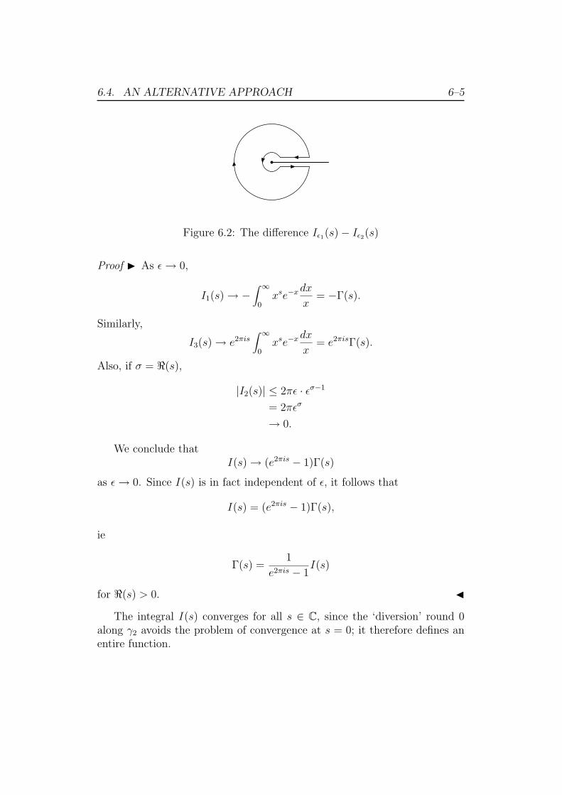
6.4. AN ALTERNATIVE APPROACH 6–5
Figure 6.2: The difference Iε1(s)− Iε2(s)
Proof I As ε→ 0,
I1(s)→ −∫ ∞
0xse−xdx
x= −Γ(s).
Similarly,
I3(s)→ e2πis∫ ∞
0xse−xdx
x= e2πisΓ(s).
Also, if σ = <(s),
|I2(s)| ≤ 2πε · εσ−1
= 2πεσ
→ 0.
We conclude thatI(s)→ (e2πis − 1)Γ(s)
as ε→ 0. Since I(s) is in fact independent of ε, it follows that
I(s) = (e2πis − 1)Γ(s),
ie
Γ(s) =1
e2πis − 1I(s)
for <(s) > 0. J
The integral I(s) converges for all s ∈ C, since the ‘diversion’ round 0along γ2 avoids the problem of convergence at s = 0; it therefore defines anentire function.
6.5. Γ(S) AS A LIMIT 6–6
Proposition 6.5. The formula
Γ(s) =1
e2πis − 1
∫γzse−z dz
z.
extends Γ(s)to a meromorphic function in the whole of C, with simple polesat s = 0,−1,−2, . . . .
Proof I Since I(s) is an entire function, the only poles of Γ(s) must arisefrom poles of
1
e2πis − 1.
But this function has simple poles with residue 1/2πi at each integer points = n ∈ Z. That is clear at s = 0, since
e2πis − 1 = 2πis+O(s2)
in the neighbourhood of s = 0; and the same result holds at s = n since thefunction is periodic with period 1.
However, I(s) = 0 if s = n > 0, since the integrand is in fact holomorphicin the uncut plane. This cancels out the pole; and in any case we know thatΓ(n+ 1) = n!.
For n = −n ≤ 0, it is still true that the integrand is holomorphic inC \ {0}, but now it has a pole of order n + 1 at s = 0. The residue of thepole is given by the coefficient of zn in e−z. Thus
I(s) =2πi
n!;
and so Γ(s) has a simple pole at s = −n with residue 1/n!, as we sawbefore. J
6.5 Γ(s) as a limit
Euler originally defined the gamma function as a limit, in the following way.
Definition 6.2. For n ∈ N, we set
Γ(s, n) =n!ns
s(s+ 1) · · · (s+ n).
Proposition 6.6. As n→∞,
Γ(s, n)→ Γ(s).
6.5. Γ(S) AS A LIMIT 6–7
Proof I Recall that (1− x
n
)n
→ e−x
as n→∞. This follows on taking logarithms, since
log(1− x
n
)n
= −n(x
n+
x2
2n2+ · · ·
)
= −t+O(1
n).
In fact, since each term −x,−x2
2n, . . . increases with n, this argument shows
that (1− x/n)n increases monotonically to e−x, for each x ≥ 0.Let
f(x, n) =
(1− x/n)n if 0 ≤ x ≤ n
0 if x > n
Thenf(x, n)→ e−x
uniformly in any finite range [0, X]; and
0 ≤ f(x, n) ≤ e−x
for all x.It follows that if <(s) > 0 then∫ n
0xs(1− 1
x
)n dx
x=∫ ∞
0xsf(x, n)
dx
x→ Γ(s)
as n→∞.
6.5. Γ(S) AS A LIMIT 6–8
But we can compute this integral by repeated integration by parts. Thus∫ n
0xs(1− 1
x
)n dx
x= Γ(s, n)
=∫ n
0xs−1
(1− x
n
)n
dx
=[xs
s
(1− x
n
)n]n0
+∫ n
0
xs
s
(1− x
n
)n−1
dx
=n
ns
∫ n
0xs(1− x
n
)n−1
dx
=n(n− 1)
n2s(s+ 1)
∫ n
0xs+1
(1− x
n
)n−2
dx
= · · ·
=n(n− 1)(n− 2) · · · 2
nn−1s(s+ 1) · · · (s+ n− 2)
∫ n
0xs+n−2
(1− x
n
)dx
=n!
nns(s+ 1) · · · (s+ n− 1)
∫ n
0xs+n−1dx
=n!
nns(s+ 1) · · · (s+ n)
[xs+n
]n0
=n!
nns(s+ 1) · · · (s+ n)ns+n
=n!ns
s(s+ 1) · · · (s+ n)
= Γ(s, n).
We have therefore established that
Γ(s, n)→ Γ(s)
as n → ∞, provided <(s) > 0. We can extend the result to all s (excepts = 0,−1,−2, . . . ) by noting that
Γ(s+ r, n) =nr+sn!
(s+ r)(s+ r + 1) · · · (s+ r + n)
= nr s(s+ 1) · · · (s+ n)
(s+ r)(s+ r + 1) · · · (s+ r + n)Γ(s, n).
Thus if n ≥ r,
Γ(s, n) =Γ(s+ r, n)
s(s+ 1) · · · (s+ r − 1)
nr
(s+ n+ 1) · · · (s+ n+ r).
6.5. Γ(S) AS A LIMIT 6–9
Now suppose <(s) > −r. From above,
Γ(s+ r, n)→ Γ(s+ r).
Moreover,
nr
(s+ n+ 1) · · · (s+ n+ r)=
1
(1 + s+1n
) · · · (1 + s+rn
→ 1
as n→∞. It follows that
Γ(s, n)→ Γ(s+ r)
s(s+ 1) · · · (s+ r − 1)= Γ(s).
We have thus extended the result to <(s) > −r, and so to the whole plane(excluding the poles s = 0,−1,−2, . . . ). J
We can re-write Γ(s, n) as
Γ(s, n) =ns
s
1
(1 + s)(1 + s2) · · · (1 + s
n).
Thus
sΓ(s, n) = ns∏
1≤m≤n
(1 +
s
m
)−1
.
We can also re-write n as
n =2
1
3
2· · · n
n− 1
=∏
1≤m≤(n−1)
(1 +
1
m
).
Thus
ns =∏
1≤m≤(n−1)
(1 +
1
m
)s
.
Hence
sΓ(s, n) =(1 +
1
n
)−s ∏1≤m≤n
{(1 +
s
m
)−1 (1 +
1
m
)s}.
Since (1 + 1n)s → 1, it follows that
∏1≤m≤n
{(1 +
s
m
)−1 (1 +
1
m
)s}→ sΓ(s).
6.6. THE SECOND IDENTITY 6–10
In other words, Γ(s) can be expressed as the infinite product
Γ(s) =1
s
∏m≥1
(1 + am),
where
1 + am =(1 +
s
m
)−1 (1 +
1
m
)s
.
This infinite product converges absolutely, since
1 + am =(1 +
s
m
)−1 (1 +
1
m
)s
=
(1− s
m+
s2
m2+O(
1
m3
)(1 +
s
m+s(s− 1)
2m2+O(
1
m3
)
= 1− s(s− 1)
2m2+O(
1
m3),
and we know of course that∑m−2 converges.
Since the series∑|am| is uniformly convergent in any compact (ie closed
and bounded) subset C not containing any of the poles, the function de-fined by the infinite product is holomorphic in C. This gives a third way ofextending Γ(s) holomorphically to the entire plane.
6.6 The second identity
Proposition 6.7. For all s ∈ C \ Z,
Γ(s)Γ(1− s) =π
sin πs.
Proof I We have
Γ(s, n)Γ(1− s, n) =ns
s(1 + s)(1 + s2) · · · (1 + s
n)
n1−s
(1− s)(1− s2) · · · (1− s
n)
1
1− s+ n
=1
s
∏1≤m≤n
(1− s2
m2
)−1n
1− s+ n
But we saw in Chapter 1 that
sin πs = πs∏(
1− s2
m2
).
It follows thatΓ(s, n)Γ(1− s, n)→ π
sin πs,
from which the result follows. J
6.7. THE THIRD IDENTITY 6–11
We shall give another proof of this result below.
Proposition 6.8. Γ(1/2) =√π.
Proof I Setting s = 1/2 in the identity above,
Γ(1/2)2 =π
sin π2
= π.
ThusΓ(1/2) = ±
√π.
Since
Γ(1/2) =∫ ∞
0x1/2e−xdx
x> 0,
it follows thatΓ(1/2) =
√π.
J
Corollary 6.2. For each n ∈ N,
Γ(n+1
2) =
1
2
3
2· · · (n− 1
2)
1√π
6.7 The third identity
We can write (2n)! as
(2n)! = (1 · 3 · 5 · · · (2n− 1)) (2 · 4 · 6 · · · (2n))
= 22n(
1
2
3
2· · · (n− 1
2))n!
= 22n Γ(n+ 12)
Γ(12)
n!.
Dividing each side by 2n,
Γ(2n) = 22n−1 Γ(n+ 12)Γ(n)
Γ(12)
ie
Γ(n)Γ(n+ 12) = 21−2n
√πΓ(2n).
This strongly suggests — but does not establish— the following result.
6.8. THE EULERIAN INTEGRAL 6–12
Proposition 6.9. For all s,
Γ(s)Γ(s+ 12) = 21−2s
√πΓ(2s).
Proof I We have
Γ(s, n)Γ(s+ 12) =
n2s+ 12 (n!)2
s(s+ 12)(s+ 1)(s+ 3
2) · · · (s+ n)(s+ n+ 1
2)
=22n+2n2s+ 1
2 (n!)2
2s(2s+ 1) · · · (2s+ 2n)(2s+ 2n+ 1)
while
Γ(2s, 2n) =(2n)2s(2n)!
2s(2s+ 1) · · · (2s+ 2n)
=22sn2s(2n)!
2s(2s+ 1) · · · (2s+ 2n).
Thus
22sΓ(s)Γ(s+ 12)
Γ(2s)=
22n+2n12 (n!)2
(2n)!
1
2s+ 2n+ 1
=22nn
12 (n− 1)!2
(2n− 1)!
2n
2s+ 2n+ 1
=22nn
12 Γ(n)2
Γ(2n)
2n
2s+ 2n+ 1.
Note that the right-hand side is independent of s, except for the factor2n/(2s+2n+1), which tends to 1 and can thus be ignored. We have to showthat the right-hand side →
√π as n→∞, ie
22nn12 Γ(n)2
Γ(2n)→√π.
It follows that if the result holds for one s then it will hold for all s.But we saw in the introduction to the Proposition that the result holds forpositive integers s = m > 0. We conclude that it holds for all s. J
6.8 The Eulerian integral
Definition 6.3. For <(u) > 0, <(v) > 0, we set
B(u, v) =∫ 1
0tu−1(1− t)v−1dt.
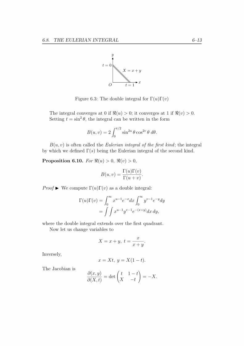
6.8. THE EULERIAN INTEGRAL 6–13
t = 0
t = 1
X = x + y
Ox
y
Figure 6.3: The double integral for Γ(u)Γ(v)
The integral converges at 0 if <(u) > 0; it converges at 1 if <(v) > 0.Setting t = sin2 θ, the integral can be written in the form
B(u, v) = 2∫ π/2
0sin2u θ cos2v θ dθ.
B(u, v) is often called the Eulerian integral of the first kind ; the integralby which we defined Γ(s) being the Eulerian integral of the second kind.
Proposition 6.10. For <(u) > 0, <(v) > 0,
B(u, v) =Γ(u)Γ(v)
Γ(u+ v).
Proof I We compute Γ(u)Γ(v) as a double integral:
Γ(u)Γ(v) =∫ ∞
0xu−1e−xdx
∫ ∞
0yv−1e−ydy
=∫ ∫
xu−1yv−1e−(x+y)dx dy,
where the double integral extends over the first quadrant.Now let us change variables to
X = x+ y, t =x
x+ y.
Inversely,x = Xt, y = X(1− t).
The Jacobian is∂(x, y)
∂(X, t)= det
(t 1− tX −t
)= −X.
6.8. THE EULERIAN INTEGRAL 6–14
Thus the integral becomes
Γ(u)Γ(v) =∫ ∞
0
∫ 1
0Xu+v−2tu−1(1− t)v−1e−XXdX dt
=∫ ∞
0Xu+v−1e−XdX
∫ 1
0tu−1(1− t)v−1dt
= Γ(u+ v)B(u, v),
as required. J
This provides an alternative proof of our second identity
Γ(s)Γ(1− s) =π
sin πs.
For suppose 0 < <(s) < 1. Then
Γ(s)Γ(1− s) = Γ(1)B(s, 1− s)
=∫ 1
0ts(1− t)−sdt
t
=∫ 1
0
(t
1− t
)s dt
x.
Let
u =t
1− t.
As t increases from 0 to 1, u increases from 0 to ∞. Also
t =u
u+ 1= 1− 1
u+ 1,
and so
dt
t=u+ 1
u
du
(u+ 1)2
=du
u(u+ 1).
Thus
Γ(s)Γ(1− s) =∫ ∞
0
us
u(u+ 1)du
Now we can play the same ‘trick’ that we used to continue Γ(s) analyti-cally:
Γ(s)Γ(1− s) =1
e2πis − 1
∫γ
zs
z(z + 1)dz,
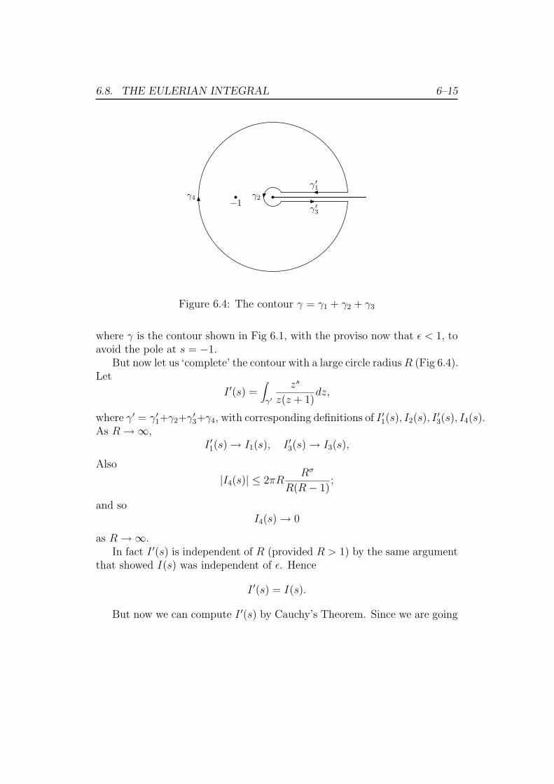
6.8. THE EULERIAN INTEGRAL 6–15
γ′1
γ2
γ′3
γ4 −1
Figure 6.4: The contour γ = γ1 + γ2 + γ3
where γ is the contour shown in Fig 6.1, with the proviso now that ε < 1, toavoid the pole at s = −1.
But now let us ‘complete’ the contour with a large circle radiusR (Fig 6.4).Let
I ′(s) =∫
γ′
zs
z(z + 1)dz,
where γ′ = γ′1+γ2+γ′3+γ4, with corresponding definitions of I ′1(s), I2(s), I
′3(s), I4(s).
As R→∞,I ′1(s)→ I1(s), I ′3(s)→ I3(s),
Also
|I4(s)| ≤ 2πRRσ
R(R− 1);
and soI4(s)→ 0
as R→∞.In fact I ′(s) is independent of R (provided R > 1) by the same argument
that showed I(s) was independent of ε. Hence
I ′(s) = I(s).
But now we can compute I ′(s) by Cauchy’s Theorem. Since we are going
6.8. THE EULERIAN INTEGRAL 6–16
round γ′ in the ‘wrong way’ (clockwise),
I ′(s) = −2πi res−1(zs
z(z + 1)
= −2πi(−1)s
−1
= 2πieπis.
We conclude that
Γ(s)Γ(1− s) =2πieπis
e2πis − 1
=2i
eπis − e−πisπ
=π
sin πs,
since sin z = (eiz − e−iz)/2i.
Chapter 7
The functional equation for ζ(s)
7.1 Analytic continuation of ζ(s)
Proposition 7.1. For <(s) > 0,
Γ(s)ζ(s) =∫ ∞
0
xs
ex − 1
dx
x.
Proof I The role of the gamma function in the theory of ζ(s) stems fromthe following result.
Lemma 16. If <(s) > 0,∫ ∞
0xse−nxdx
x= n−sΓ(s).
Proof I On making the change of variable y = nx,∫ ∞
0xse−nxdx
x=∫ ∞
0n−syse−y dy
y
= n−sΓ(s).
J
7–1
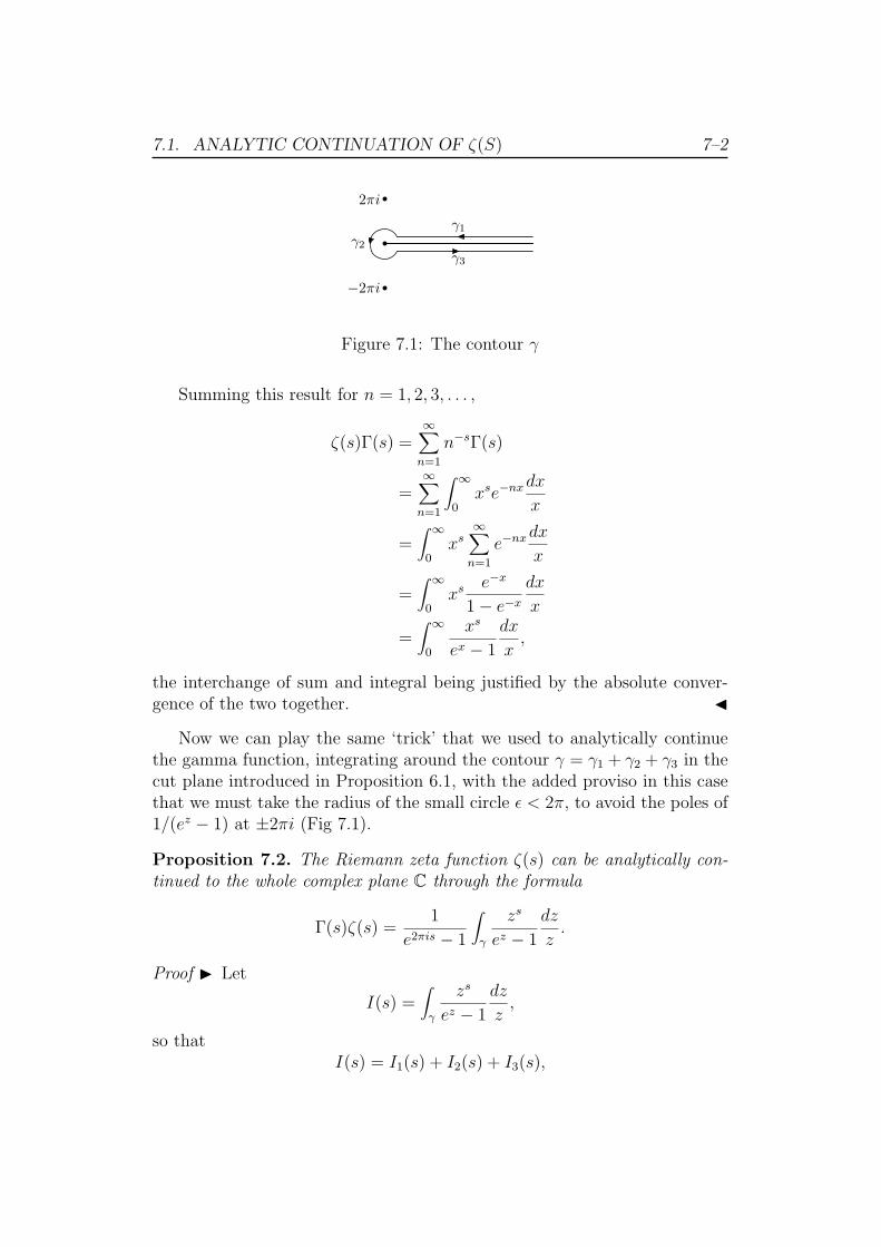
7.1. ANALYTIC CONTINUATION OF ζ(S) 7–2
γ1
γ2
γ3
2πi
−2πi
Figure 7.1: The contour γ
Summing this result for n = 1, 2, 3, . . . ,
ζ(s)Γ(s) =∞∑
n=1
n−sΓ(s)
=∞∑
n=1
∫ ∞
0xse−nxdx
x
=∫ ∞
0xs
∞∑n=1
e−nxdx
x
=∫ ∞
0xs e−x
1− e−x
dx
x
=∫ ∞
0
xs
ex − 1
dx
x,
the interchange of sum and integral being justified by the absolute conver-gence of the two together. J
Now we can play the same ‘trick’ that we used to analytically continuethe gamma function, integrating around the contour γ = γ1 + γ2 + γ3 in thecut plane introduced in Proposition 6.1, with the added proviso in this casethat we must take the radius of the small circle ε < 2π, to avoid the poles of1/(ez − 1) at ±2πi (Fig 7.1).
Proposition 7.2. The Riemann zeta function ζ(s) can be analytically con-tinued to the whole complex plane C through the formula
Γ(s)ζ(s) =1
e2πis − 1
∫γ
zs
ez − 1
dz
z.
Proof I Let
I(s) =∫
γ
zs
ez − 1
dz
z,
so thatI(s) = I1(s) + I2(s) + I3(s),
7.1. ANALYTIC CONTINUATION OF ζ(S) 7–3
where I1(s), I2(s), I3(s) denote the corresponding integrals along γ1, γ2, γ3.As in Section 6.3, I(s) is independent of ε, by Cauchy’s Theorem. And asthere,
zs = xs = es log x
at z = x on the upper edge of the cut, while
zs = es(log x+2πi) = e2πisxs
at z = x on the lower edge of the cut. Thus
I1(s) + I3(s) = (e2πis − 1)∫ ∞
ε
xs
ex − 1
dx
x
→ (e2πis − 1)ζ(s) as ε→ 0,
by Proposition 7.1.On the other hand, the function
f(z) =z
ez − 1
is holomorphic, and so bounded, in |z| ≤ π, say
|f(z)| ≤ C,
ie
| 1
ez − 1| ≤ C|z|−1.
Hence
|I2(s)| ≤ 2πCεσ−1.
Thus if <(s) > 1 thenI2(s)→ 0 as ε→ 0.
Since I(s) is independent of ε, it follows that
I(s) = (e2πis − 1)ζ(s),
ie
ζ(s) =1
e2πis − 1I(s).
J
7.2. THE FUNCTIONAL EQUATION 7–4
The following alternative form of this result is often more convenient.
Corollary 7.1. For all s,
ζ(s) =Γ(1− s)
2πie−πis
∫γ
zs
ez − 1
dz
z.
Proof I By Proposition 6.7,
Γ(s)Γ(1− s) =π
sin πs.
But
e2πis−1 = eπis(eπis − e−πis
)= 2ieπis sin πs.
Thus
ζ(s) =1
Γ(s)(e2πis − 1)I(s)
=Γ(1− s)
2πie−πisI(s).
J
Proposition 7.3. The only pole of ζ(s) in the entire complex plane C is thesimple pole (with residue 1) at s = 1.
Proof I ThefunctionΓ(1 − s) has poles at s = 1, 2, 3, . . . , since Γ(s) haspoles at s = 0,−1,−2, . . . . On the other hand, the function I(s) is entire, asis e−πis.
It follows from the Corollary to the last Proposition that ζ(s) can onlyhave poles at s = 1, 2, 3, . . . . But we know that ζ(s) is holomorphic for<(s) > 1. Thus the only possible pole is at s = 1, and we already know thatthere is a simple pole there with residue 1. J
7.2 The functional equation
Proposition 7.4. The Riemann zeta function ζ(s) satisfies the functionalequation
ζ(1− s) = 2 cos πs2
(2π)−sΓ(s)ζ(s).
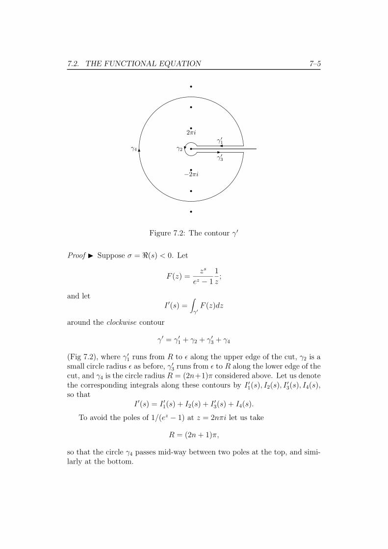
7.2. THE FUNCTIONAL EQUATION 7–5
γ′1
γ2
γ′3
γ4
2πi
−2πi
Figure 7.2: The contour γ′
Proof I Suppose σ = <(s) < 0. Let
F (z) =zs
ez − 1
1
z;
and letI ′(s) =
∫γ′F (z)dz
around the clockwise contour
γ′ = γ′1 + γ2 + γ′3 + γ4
(Fig 7.2), where γ′1 runs from R to ε along the upper edge of the cut, γ2 is asmall circle radius ε as before, γ′3 runs from ε to R along the lower edge of thecut, and γ4 is the circle radius R = (2n+1)π considered above. Let us denotethe corresponding integrals along these contours by I ′1(s), I2(s), I
′3(s), I4(s),
so thatI ′(s) = I ′1(s) + I2(s) + I ′3(s) + I4(s).
To avoid the poles of 1/(ez − 1) at z = 2nπi let us take
R = (2n+ 1)π,
so that the circle γ4 passes mid-way between two poles at the top, and simi-larly at the bottom.
7.2. THE FUNCTIONAL EQUATION 7–6
As n→∞ (and so R→∞),
I ′1(s)→ I1(s), I′3(s)→ I3(s),
On the other hand, we shall show that, since <(s) < 0,
I4(s)→ 0
as n→∞. It will follow that
I ′(s)→ I(s).
The function
f(z) =1
ez − 1
has poles atz = 2nπi (n ∈ Z).
The following Lemma shows that provided we keep a reasonable distanceaway from the poles, the function f(z) will remain reasonably small.
Lemma 17. There is a constant C such that
1
|ez − 1|≤ C.
provided|z − 2nπi| ≥ 1
for all n ∈ Z.
Proof I Since f(z) = 1/(ez − 1) is periodic with period 2πi, it is sufficientto consider its value in the strip
S = {z = x+ iy : −π ≤ y ≤ π}
outside the diskD = {z : |z| ≤ 1}
(Fig 7.3).The function
g(z) = zf(z) =z
ez − 1
is holomorphic in S, and is therefore bounded in any finite part of this strip,say
|g(z)| ≤ c
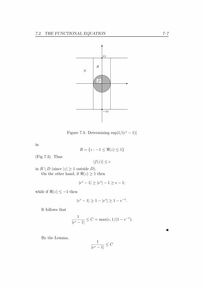
7.2. THE FUNCTIONAL EQUATION 7–7
R
S
πi
−πi
D
Figure 7.3: Determining sup|1/(ez − 1)|
inR = {z : −1 ≤ <(z) ≤ 1}
(Fig 7.3). Thus|f(z)| ≤ c
in R \D (since |z| ≥ 1 outside D).On the other hand, if <(z) ≥ 1 then
|ez − 1| ≥ |ez| − 1 ≥ e− 1;
while if <(z) ≤ −1 then
|ez − 1| ≥ 1− |ez| ≥ 1− e−1.
It follows that
1
|ez − 1|≤ C = max(c, 1/(1− e−1).
J
By the Lemma,1
|ez − 1|≤ C
7.2. THE FUNCTIONAL EQUATION 7–8
on the large circle γ4; while|zs| = Rσ
on this circle. Hence
|I4(s)| ≤ 2πCRσ
→ 0 as n→∞,
since σ = <(s) < 0.It follows that
I ′(s)→ I(s) =(e2πis − 1
)Γ(s)ζ(s)
as n→∞.But now. since the contour γ′ is closed, we can compute the integral
I ′(s) by Cauchy’s Theorem, from the residues of F (z) at its poles within thecontour. Since the contour runs in the ‘wrong’ direction (clockwise ratherthan anti-clockwise), we must negate the sum. Thus
I ′(s) = −2πi∑
0<m≤n
(res2mπi(F ) + res−2mπi(F )) .
In the neighbourhood of z = 0,
f(z) =1
ez − 1=
1
z + z2/2 + · · ·=
1
z+ h(z),
where h(z) is holomorphic at z = 0. It follows that f(z) has a simple polewith residue 1 at z = 0. Therefore, since f(z) is periodic with period 2πi, ithas a simple pole with residue 1 at z = 2nπi for each n ∈ Z. Thus
res2nπi(F ) =(2nπi)s
2nπi, res−2nπi(F ) =
(−2nπi)s
−2nπi.
We must take care to compute the powers correctly. Recall that if
z = reiθ (0 ≤ θ ≤ 2π)
then we must takezs = rseiθs.
Thusz = 2nπi = 2nπeiπ/2 =⇒ zs = (2nπ)seπis/2,
whilez = −2nπi = 2nπe3πi/2 =⇒ zs = (2nπ)se3πis/2.
7.2. THE FUNCTIONAL EQUATION 7–9
It follows that
I ′(s) = −2πi∑
0<m≤n
(2nπ)s
(eπi/2
2nπi+
e3πi/2
−2nπi
)
= (2π)s∑
0<m≤n
ns−1(e3πi/2 − eπi/2
).
Since ∑ns−1 = ζ(1− s),
we conclude that
Γ(s)ζ(s) =1
e2πis − 1I(s)
=1
e2πis − 1lim
n→∞I ′(s)
=e3πis/2 − eπis/2
e2πis − 1(2π)sζ(1− s)
=eπis/2 − e−πis/2
eπis − e−πis(2π)sζ(1− s)
=1
eπis/2 + e−πis/2(2π)sζ(1− s)
=1
2 cos(πs/2)(2π)sζ(1− s),
ie2 cos(πs/2)Γ(s)ζ(s) = (2π)sζ(1− s).
All this was on the assumption that <(s) < 0. But now it follows byanalytic continuation that the result holds for all s ∈ C. J
The functional equation can be re-written in various ways, using theproperties of Γ(s) established in Chapter 6. In particular we can express itin a form invariant under the transformation s→ 1−s. (In geometric terms,this transformation describes reflection in the point s = 1/2.)
Proposition 7.5. Let
ξ(s) = s(s− 1)π−s2 Γ(
s2
)ζ(s).
Then ξ(s) is an entire function; and
ξ(1− s) = ξ(s).
7.2. THE FUNCTIONAL EQUATION 7–10
Proof I The function Γ(s/2) has poles at s = 0,−2,−4, . . . , while ζ(s) haszeros at s = −2,−4, . . . . This leaves a pole at s = 0 which is cancelled bythe zero of the factor s, In addition, the pole of ζ(s) at s = 1 is cancelled bythe zero of the factor s− 1. Thus all possible poles of ξ(s) are accounted for,and this function must be entire.
By the second gamma function identity (Proposition 6.7), with (1− s)/2in place of s,
Γ(
1−s2
)Γ(
1+s2
)=
π
sin π(1−s)2
=π
cos πs2
,
since sin(π/2− τ) = cos τ .By the third gamma function identity (Proposition 6.9), with s/2 in place
of s,Γ(
s2
)Γ(
1+s2
)= 21−sπ
12 Γ(s).
Dividing one relation by the other,
Γ( s2)
Γ(1−s2
)= 21−s cos
πs
2Γ(s)π−
12 .
But the functional equation can be written
ζ(1− s)ζ(s)
= 21−s cosπs
2Γ(s)π−s
=Γ( s
2)
Γ(1−s2
)π
12−s.
Thus if we set
η(s) = Γ(s
2)ζ(s)
then
η(1− s)η(s)
= π12−s.
But now if we set
θ(s) = πs2
7.3. THE BEHAVIOUR OF ζ(S) FOR <(S) ≤ 0 7–11
then
θ(1− s)θ(s)
= π12−s.
Hence
η(1− s)η(s)
=θ(1− s)θ(s)
ie
β(1− s) = β(s),
where
β(s) = η(s)θ(s)
= π−s2 Γ(
s2
)ζ(s).
We conclude that, since the function s(s − 1) is invariant under s 7→ 1 − s(we include it to remove the pole at s = 1),
ξ(s) = s(s− 1)β(s)
= s(s− 1)π−s2 Γ(
s2
)ζ(s)
satisfiesξ(1− s) = ξ(s).
J
7.3 The behaviour of ζ(s) for <(s) ≤ 0
The functional equation allows us to determine how ζ(s) behaves ‘on the farside’ of the critical strip 0 ≤ <(s) ≤ 1; for the map
s 7→ 1− 2
sends the left-hand half-plane <(s) < 0 into the half-plane <(s) > 1, whereζ(s) is well-behaved.
We already know that ζ(s) has no poles in <(s) ≤ 0, by Proposition 7.3.It does however have zeros, as we shall see.
Proposition 7.6. The Riemann zeta function ζ(s) has simple zeros at s =−2,−4,−6, . . . . It has no other zeros (or poles) in <(s) ≤ 0.
7.4. THE VALUES OF ζ(2N) 7–12
Proof I Since π−s/2 and Γ(s/2) have no zeros anywhere, it follows that anyzero of
ξ(s) = s(s− 1)πs2 Γ(
ss
)ζ(s)
must be a zero of ζ(s), except possibly for s = 0, 1.At s = 1, ζ(s) has a simple pole which is cancelled out by the zero of
s − 1. Thus ξ(1) 6= 0; and since ξ(0) = ξ(1) by the functional equationξ(1− s) = ξ(s), it follows that ξ(0) 6= 0. Thus
ξ(s) = 0 =⇒ ζ(s) = 0.
Now we know that ζ(s) has no zeros in <(s) ≥ 1 by Propositions 3.4 and3.8. Hence ξ(s) has no zeros in <(s) ≥ 1. Thus ξ(s) has no zeros in <(s) ≤ 0,since ξ(1− s) = ξ(s).
It follows that ζ(s) has zeros in <(s) ≤ 0 just at those points wheres(s− 1)Γ(s/2) has poles. Now Γ(s/2) has simple poles at s = 0,−2,−4, . . . ;but the pole at s = 0 is cancelled by the zero of s at this point. We concludethat ζ(s) has simple zeros at s = −2,−4,−6, . . . , and that these are the onlyzeros of ζ(s) in <(s) ≤ 0. J
7.4 The values of ζ(2n)
The functional equation allows us to express ζ(2n) in terms of ζ(1 − 2n).Although at first sight this might seem a step backwards, it turns out that thelatter can be determined with relative ease, using Cauchy’s Residue Theorem.
Interestingly, the argument only works for even values; there seem to beno simple expressions for
ζ(3), ζ(5), ζ(7), . . . .
7.4.1 The Bernouilli numbers
Our formulae for ζ(2n) involve the Bernouilli numbers, rational numberswhich occur in many mathematical formulae.
Definition 7.1. The Bernouilli numbers Bn(n ∈ N) are defined by
z
ez − 1=∑n∈N
Bizi
i!.
Remarks. 1. Different authors use slightly different notations for the Bernouillinumbers. As we shall see, the odd Bernouilli numbers all vanish afterthe first. What we call B2n is sometimes denoted by Bn.
7.4. THE VALUES OF ζ(2N) 7–13
Again, it will follow from our formulae for ζ(2n) that B2, B4, B6, . . . arealternatively positive and negative. Sometimes Bn is used to denote theabsolute value, so that Bn ≥ 0 for all n.
However, we shall stick with the definition above.
2. We can compute the Bernouilli numbers recursively from the identity(1 + 1
2z + 1
6z2 + 1
24z3 + 1
120z4 + · · ·
) (B0 +B1z + 1
2B2z
2 + 16B3z
3 + 124B4z
4 + · · ·)
= 1.
Comparing constant terms,
B0 = 1.
Comparing coefficients of z, z2, z3, z4,
B1 + 12B0 = 0 =⇒ B1 = −1
2,
12B2 + 1
2B1 + 1
6B0 = 0 =⇒ B2 = −1
6,
16B3 + 1
4B2 + 1
6B1 + 1
24B0 = 0 =⇒ B3 = 0,
124B4 + 1
12B3 + 1
12B2 + 1
24B1 + 1
24B0 = 0 =⇒ B4 = − 1
30.
Proposition 7.7. The odd Bernouilli numbers after B1 all vanish:
B2n+1 = 0 (n = 1, 2, 3, . . . ).
Proof I Let
f(z) =z
ez − 1.
Then
f(−z) =−z
e−z − 1
=zez
ez − 1.
Thusf(z)− f(−z) = −z.
On the other hand,
f(z)− f(−z) = 2∑
n odd
Bnzn
n!.
It follows that
B1 = −1
2, B3 = B5 = · · · = 0.
J
7.4. THE VALUES OF ζ(2N) 7–14
7.4.2 Determining ζ(1− 2n)
Proposition 7.8. For n = 1, 2, 3, . . . ,
ζ(1− 2n) = −B2n
2n.
Proof I By the Corollary to Proposition 7.2, setting s = 1− 2n,
ζ(1− 2n) =Γ(2n)
2πie−πi(1−2n)
∫γ
z−2n
ez − 1dz.
Now the function
F (z) =z−2n
ez − 1
is meromorphic in the complex plane. In particular, the values of F (z) atz = x on the upper and lower edges of the cut coincide. It follows that theintegrals of F (z) along γ1 and γ3 cancel out, leaving
ζ(1− 2n) = −Γ(2n)
2πiI2,
where
I2 =∫
γ2
F (z)dz
= 2πi res0(F ),
by Cauchy’s Theorem.But
F (z) =z−2n
ez − 1
= z−2n−1 z
ez − 1
= z−2n−1∑r≥0
Brzr
r!
=∑r≥0
Brzr−2n−1
r!.
By definition, res0(F ) is the coefficient of z−1 in this expansion. Thus
res0(F ) =B2n
(2n)!.
7.4. THE VALUES OF ζ(2N) 7–15
Hence
ζ(1− 2n) =Γ(2n)
2πi(−2πi)
B2n
(2n)!
= −(2n− 1)!
(2n)!B2n
= −B2n
2n.
J
7.4.3 Determining ζ(2n)
Proposition 7.9. For n = 1, 2, 3, . . . ,
ζ(2n) = (−1)n−122n−1π2n B2n
(2n)!.
Proof I By the functorial equation, Proposition 7.4,
ζ(1− 2n) = 2 cos 2πn2
(2π)−2nΓ(2n)ζ(2n).
Thus
ζ(2n) = (−1)n22n−1π2n ζ(1− 2n)
Γ(2n)
= (−1)n−122n−1π2n B2n
2nΓ(2n)
= (−1)n−122n−1π2n B2n
(2n)!.
J
For n = 1 this gives
ζ(2) = 1 +1
22+
1
32+ · · · = π2B2 =
π2
6,
a result which is probably familiar, and which can be proved in several ways.For n = 2 it gives
ζ(4) = 1 +1
24+
1
34+ · · · = −1
3π4B4 =
π4
90.
7.5. POSTSCRIPT 7–16
7.5 Postscript
In his seminal paper (Appendix B), Riemann gave a second proof of thefunctional equation. Although at first sight this seems more complicated thanhis first proof (given above) it has turned out to have far greater significance.
By Lemma 16, with πn2 in place of n,
Γ(s)(πn2)−s =∫ ∞
0xse−πn2xdx
x.
Summing over n, as before,
Γ(s)π−sζ(2s) =∫ ∞
0zsψ(x)− 1
2
dx
x,
where
ψ(x) =∞∑−∞
e−πn2x.
Some 20 years before Riemann’s work, Jacobi had published a study ofthe function ψ(x), in the course of which he showed that ψ(x) satisfies thefunctional equation
ψ(
1x
)= x−
12ψ(x).
It is a straightforward matter to derive the functional equation for ζ(s) fromthis.
It follows from Jacobi’s identity that the theta function
θ(x) = ψ(x/i) =∑
epiin2x
satisfies the equation
θ(
1x
)=√
ixθ(x).
It is clear that θ(x) is also periodic with period 1:
θ(x+ 1) = θ(x).
Now the transformations x 7→ 1/x, x 7→ x+1 generate the modular groupconsisting of the transformations
z 7→ az + b
cz + d(a, b, c, d ∈ Z, ad− bc = 1).
This group can be identified with the group of 2× 2 matrices
SL2(Z) = {(a bc d
): ad− bc = 1}
7.5. POSTSCRIPT 7–17
The relation between zeta functions and modular functions — functionsinvariant, or nearly invariant, under the modular group — has proved remark-ably fruitful. Andrew Wiles’ proof of Fermat’s Last Theorem, for example,was based on this correspondence.
Another advantage of this approach is that it leads to a functional equa-tion for Lχ(s), although one relating Lχ(1 − s) to Lχ(s), where χ is theconjugate character to χ, given by
χ(a) = χ(a) = χ(a−1).
This identity in turn suggests the Generalised Riemann Hypothesis, whichasserts that the zeros of Lχ(s) in the critical strip 0 < <(s) < 1 all lie on theline <(s) = 1/2.
Incidentally, the zeta functions ζk(s) of number fields k, which we brieflyalluded to earlier, can all be expressed in terms of the Riemann zeta functionζ(s) and the L-functions Lchi(s); and the Riemann Hypothesis for ζk(s)would follow from the Generalised Riemann Hypothesis. In that sense, theGeneralised Riemann Hypothesis is as general as one would wish.
Contents
1 Euler’s Product Formula 1–11.1 The Product Formula . . . . . . . . . . . . . . . . . . . . . . . 1–11.2 Infinite products . . . . . . . . . . . . . . . . . . . . . . . . . 1–2
1.2.1 Definition . . . . . . . . . . . . . . . . . . . . . . . . . 1–21.2.2 The complex logarithm . . . . . . . . . . . . . . . . . . 1–31.2.3 Convergence . . . . . . . . . . . . . . . . . . . . . . . . 1–4
1.3 Proof of the product formula . . . . . . . . . . . . . . . . . . . 1–61.4 Euler’s Theorem . . . . . . . . . . . . . . . . . . . . . . . . . 1–7
2 Dirichlet series 2–12.1 Definition . . . . . . . . . . . . . . . . . . . . . . . . . . . . . 2–12.2 Convergence . . . . . . . . . . . . . . . . . . . . . . . . . . . . 2–22.3 Absolute convergence . . . . . . . . . . . . . . . . . . . . . . . 2–52.4 The Riemann zeta function . . . . . . . . . . . . . . . . . . . 2–72.5 The Riemann-Stieltjes integral . . . . . . . . . . . . . . . . . . 2–12
2.5.1 Functions of bounded variation . . . . . . . . . . . . . 2–142.5.2 Discontinuities . . . . . . . . . . . . . . . . . . . . . . 2–192.5.3 Integration by parts . . . . . . . . . . . . . . . . . . . 2–242.5.4 The abscissa of convergence revisited . . . . . . . . . . 2–262.5.5 Analytically continuing ζ(s) . . . . . . . . . . . . . . . 2–27
2.6 The relation between An and σ0 . . . . . . . . . . . . . . . . . 2–302.7 Dirichlet series with positive terms . . . . . . . . . . . . . . . 2–32
3 The Prime Number Theorem 3–13.1 Statement of the theorem . . . . . . . . . . . . . . . . . . . . 3–13.2 Preview of the proof . . . . . . . . . . . . . . . . . . . . . . . 3–33.3 Logarithmic differentiation . . . . . . . . . . . . . . . . . . . . 3–73.4 From π(x) to θ(x) . . . . . . . . . . . . . . . . . . . . . . . . . 3–83.5 The zeros of ζ(s) . . . . . . . . . . . . . . . . . . . . . . . . . 3–103.6 The Tauberian theorem . . . . . . . . . . . . . . . . . . . . . . 3–153.7 Proof . . . . . . . . . . . . . . . . . . . . . . . . . . . . . . . . 3–20
0–18
CONTENTS 0–19
4 The Dirichlet L-functions 4–14.1 Characters of a finite abelian group . . . . . . . . . . . . . . . 4–1
4.1.1 Definition of a character . . . . . . . . . . . . . . . . . 4–14.1.2 The dual group A∗ . . . . . . . . . . . . . . . . . . . . 4–34.1.3 Sums over elements . . . . . . . . . . . . . . . . . . . . 4–64.1.4 Sums over characters . . . . . . . . . . . . . . . . . . . 4–74.1.5 Functions on a finite abelian group . . . . . . . . . . . 4–8
4.2 Multiplicative characters modm . . . . . . . . . . . . . . . . . 4–104.2.1 Characters and multiplicative functions . . . . . . . . . 4–17
4.3 Dirichlet’s L-functions . . . . . . . . . . . . . . . . . . . . . . 4–19
5 Dirichlet’s Theorem 5–15.1 Preview of the proof . . . . . . . . . . . . . . . . . . . . . . . 5–25.2 From πr,m(x) to θr,m(x) . . . . . . . . . . . . . . . . . . . . . . 5–55.3 Picking out the residue class . . . . . . . . . . . . . . . . . . . 5–55.4 The zeros of Lχ(s) . . . . . . . . . . . . . . . . . . . . . . . . 5–65.5 Proof of Dirichlet’s Theorem . . . . . . . . . . . . . . . . . . . 5–13
6 The gamma function 6–16.1 Definition . . . . . . . . . . . . . . . . . . . . . . . . . . . . . 6–16.2 The first identity . . . . . . . . . . . . . . . . . . . . . . . . . 6–26.3 Analytic continuation . . . . . . . . . . . . . . . . . . . . . . . 6–26.4 An alternative approach . . . . . . . . . . . . . . . . . . . . . 6–36.5 Γ(s) as a limit . . . . . . . . . . . . . . . . . . . . . . . . . . . 6–66.6 The second identity . . . . . . . . . . . . . . . . . . . . . . . . 6–106.7 The third identity . . . . . . . . . . . . . . . . . . . . . . . . . 6–116.8 The Eulerian integral . . . . . . . . . . . . . . . . . . . . . . . 6–12
7 The functional equation for ζ(s) 7–17.1 Analytic continuation of ζ(s) . . . . . . . . . . . . . . . . . . . 7–17.2 The functional equation . . . . . . . . . . . . . . . . . . . . . 7–47.3 The behaviour of ζ(s) for <(s) ≤ 0 . . . . . . . . . . . . . . . 7–117.4 The values of ζ(2n) . . . . . . . . . . . . . . . . . . . . . . . . 7–12
7.4.1 The Bernouilli numbers . . . . . . . . . . . . . . . . . 7–127.4.2 Determining ζ(1− 2n) . . . . . . . . . . . . . . . . . . 7–147.4.3 Determining ζ(2n) . . . . . . . . . . . . . . . . . . . . 7–15
7.5 Postscript . . . . . . . . . . . . . . . . . . . . . . . . . . . . . 7–16