CHAPTER 1: ELEMENTS OF WAVE MECHANICS

1.1 Introduction. 1.2 Black body radiation. 1.2.1 Experimental observation of black body radiation. 1.2.2 Laws of black body radiation. 1.2.3 Stefan – Boltzmann radiation law. 1.2.4 Wien’s law. 1.2.5 Rayleigh – Jean’s law. 1.2.6 Planck’s radiation law. 1.2.7 Derivation of Wien’s law from Planck’s law. 1.2.8 Derivation of Rayleigh – Jean’s law from Planck’s

law. 1.3 Photoelectric effect. 1.4 Compton effect. 1.5 Matter waves and de Broglie hypothesis

1.5.1 Davisson and Germer experiment.

1.5.2 G.P.Thomson experiment

1.5.3 Wave packet and de Broglie wave

1.6 Phase and group velocities

1.6.1 Relation between phase velocity and group velocity

1.6.2 Relationbetween group velocity and particle

velocity (Velocity of de Broglie waves)

1.6.3 Derivation of de Broglie relation

1.7 Uncertainty principle.

1.7.1 Origin and nature of the principle.

1.7.2 An illustration of uncertainty principle.

1.7.3 Physical significance of uncertainty principle.

1.8 Wave mechanics.

1.8.1 Characteristics of wave function.

1.8.2 Physical significance of wave function.

1.8.3 Schrodinger’s wave equation.

1.8.4 Eigen values and Eigen functions.

1.9 Applications of Schrodinger’s equation.

1.9.1 Case of a free particle.

1.9.2 Particle in a box.

1.9.3 Finite potential well

1.9.4 Tunnel effect

1.9.5 Examples of tunneling across a finite barrier.

1.9.6 Theoretical interpretation of tunneling

1.9.7 Harmonic oscillator.

1.9.8 Practical applications of Schrodinger’s wave

equation.

Numerical examples

Exercise

1.1 INTRODUCTION:

The nineteenth century was a very eventful period as

far as Physics is concerned. The pioneering work on

dynamics by Newton, on electromagnetic theory by

Maxwell, laws of thermodynamics and kinetic theory were

successful in explaining a wide variety of phenomena.

Even though a majority of experimental evidence agreed

with the classical physics, a few experiments gave

results that could not be explained satisfactorily.

These few experiments led to the development of modern

physics. Modern physics refers to the development of

the theory of relativity and the quantum theory.

Inability of the classical concepts to explain certain

experimental observations, especially those involving

subatomic particles, led to the formulation and

development of modern physics. Early twentieth century

saw the development of modern physics. The pioneering

work of Einstein, Planck, Compton, Roentgen, Born and

others formed the basis of modern physics. The dual

nature of matter proposed by de Broglie was confirmed

by experiments. The wave mechanics and quantum

mechanics were later shown to be identical in their

mathematical formulation. The validity of classical

concepts was explained to be the result of an

extrapolation of modern theories to classical

situations. In the present chapter, experimental

observations of three important phenomena – black body

radiation, photoelectric effect and Compton effect –

considered as the beginning of modern physics, are

briefly described.

1.2 BLACK BODY RADIATION:

When radiation is incident on material objects, it

is either absorbed, reflected or transmitted. These

processes are dependent on the radiation and the object

involved. An object that is capable of absorbing all

radiation incident on it is called a black body.

Practically, we cannot have a perfect black body but

can have objects that are only close to a black body.

For example, a black body can be approximated by a

hollow object with a very small hole leading to the

inside of the object. Any radiation that enters the

object through the hole gets trapped inside and will be

reflected by the walls of the cavity till it is

absorbed. Objects that absorb a particular wavelength

of radiation are also found to be a good emitter of

radiation of that particular wavelength. Hence, a

black body is also a good emitter of all radiations it

has absorbed.

Emissions from objects depend on the temperature

of the object. It has been observed that the energy

emitted from objects increases as the temperature of

the object is increased. Laws of radiation have been

formulated to explain the emission of energy by objects

maintained at specific temperatures.

1.2.1 Experimental observation of black body radiation:

Experiments have been carried out to study the

distribution of energy emitted by a practical blackbody

as a function of wavelength and temperature. Figure 1.1

.

1.1 Distribution of emitted energy as a function of wavelength and temperature for a black body.

shows the distribution curves in which the energy

density Eλ is plotted as a function of wavelength at

different temperatures of the black body. Energy

density is defined as the energy emitted by the black

body per unit area of the surface. The important

features of these distribution curves may be summarized

as follows:

(i) The energy vs wavelength curve at a given

temperature shows a peak indicating that the emitted

intensity is maximum at a particular wavelength and

decreases as we move away from the peak.

(ii) An increase in temperature results in an increase

in the total energy emitted and also the energy emitted

at all wavelengths.

(iii) As the temperature increases, the peak shifts to

lower wavelengths. In other words, at higher

temperatures, maximum energy is emitted at lower

wavelengths.

1.2.2 Laws of black body radiation:

The initial attempts to explain black body

radiation were based on classical theories and were

found to be limited in application. They could not

explain the entire spectrum of the radiation

satisfactorily.

1.2.3 Stefan Boltzmann radiation law:

It states that the total energy density Eo of

radiation emitted from a black body is directly

proportional to the fourth power of its absolute

temperature T. Energy density E0 is defined as the

total of all the energy emitted at all wavelengths per

unit area of the emitter surface.

Eo ∝ T4

or Eo = σ T4 (1.1)

where σ is a constant called Stefan’s constant. It

has a numerical value equal to 5.67 x 10-8 watt m-2 K-4 .

This law was suggested empirically by Stefan and later

derived by Boltzmann on thermodynamic considerations.

The law agrees well with the experimental results.

1.2.4 Wien’s Laws:

Wien’s displacement law states that the wavelength

λm corresponding to the maximum emissive energy

decreases with increasing temperature.

i.e. λm ∝ 1/T or λm T = b (1.2)

where b is called the Wien’s constant and is equal to

2.9 x 10-3 mK. The energy density emitted by a black

body in the wavelength range λ and λ + dλ is given by

Eλ dλ = c1 λ-5 exp(-c2/λT) dλ (1.3)

where c1 and c2 are constants. This is known as Wien’s

distribution law. This law holds good for smaller

values of λ but does not fit the experimental curves

for higher values of λ (fig 1.2).

1.2 Comparison of experimental distribution curve with Wien’s law.

1.2.5 Rayleigh – Jean’s law:

According to this law, the energy density emitted

by a black body in the wavelength range λ And λ + dλ is

given by

Eλ dλ = 8πkT λ4

dλ (1.4)

This equation does not show any peak in the energy

value but the energy goes on increasing with decrease

in wavelength. The total energy emitted is infinite

for all temperatures above 0 K.

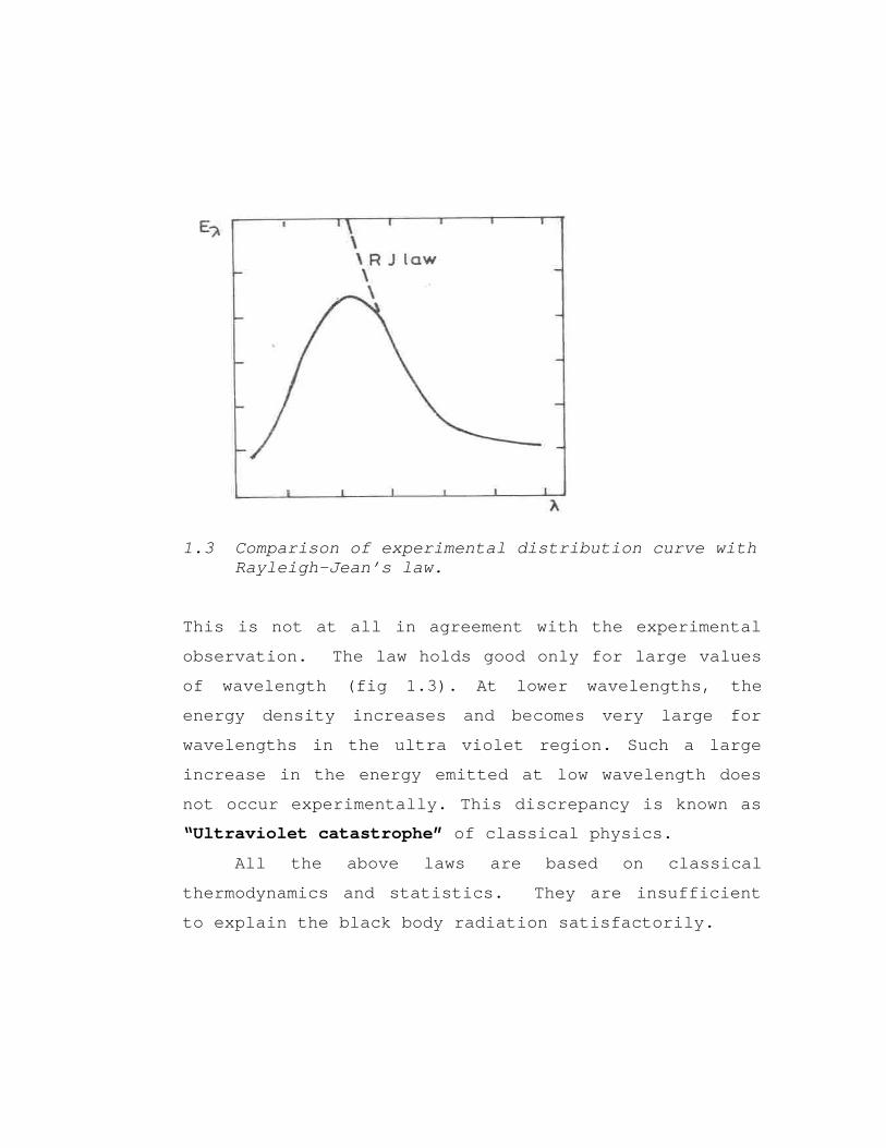
1.3 Comparison of experimental distribution curve with Rayleigh-Jean’s law.

This is not at all in agreement with the experimental

observation. The law holds good only for large values

of wavelength (fig 1.3). At lower wavelengths, the

energy density increases and becomes very large for

wavelengths in the ultra violet region. Such a large

increase in the energy emitted at low wavelength does

not occur experimentally. This discrepancy is known as

“Ultraviolet catastrophe” of classical physics.

All the above laws are based on classical

thermodynamics and statistics. They are insufficient

to explain the black body radiation satisfactorily.

1.2.6 Planck’s radiation law:

This law is based on quantum theory. Max Planck

proposed that atoms or molecules absorb or emit

radiation in quanta or small energy packets called

photons. Energy of each photon can be expressed as

E = hν

where ν is the frequency of the radiation corresponding

to the energy E, h is a constant called Planck’s

constant and is equal to 6.63 x 10-34 Js. Light quanta

are indistinguishable from each other and there is no

restriction on the number of quanta having the same

energy. In other words, Pauli’s exclusion principle is

not applicable to them. The quantum statistics

applicable to photons is Bose-Einstein statistics.

Considering all the energy emitted by the black body in

the form of photons of different energy, Planck applied

Bose - Einstein statistics to obtain the energy

distribution of photons. Accordingly, the energy

density emitted in the wavelength range λ and(λ + dλ)

is given by

Eλ dλ = 8πhc _____1 ___ λ5 (ehc/λkT –1)

dλ (1.5)

This distribution agrees well with the

experimental observation of black body radiation and is

valid for all wavelengths. Further, it reduces to

Wien’s law for lower wavelength region and to Rayleigh

– Jean’s law for higher wavelength region.

1.2.7 Derivation of Wien’s law from Planck’s law:

When λ is small, we can consider

ehc/λkT > 1

∴ [ehc/λkT - 1 ] ≈ ehc/λkT

Substituting in equation (1.5), we get

Eλ dλ = 8πhc . 1__ λ5 (ehc/λkT)

. dλ

i.e. Eλ dλ = c1 λ-5 . exp(-c2/λT) dλ (1.6) where c1 = 8πhc and c2 = hc/k

Equation (1.6) is the Wien’s law.

1.2.8 Derivation of Rayleigh – Jean’s law from Planck’s

law.

When λ is large, hc λkT

< 1.

∴ [ehc/λkT - 1 ] ≈ hc / λkT Substituting in equation (1.5), we get

Eλ dλ = 8πhc . λkT λ5 hc

. dλ

i.e. Eλ dλ = 8πkT λ4

dλ (1.7)

Equation (1.7) is the Rayleigh – Jean’s law.

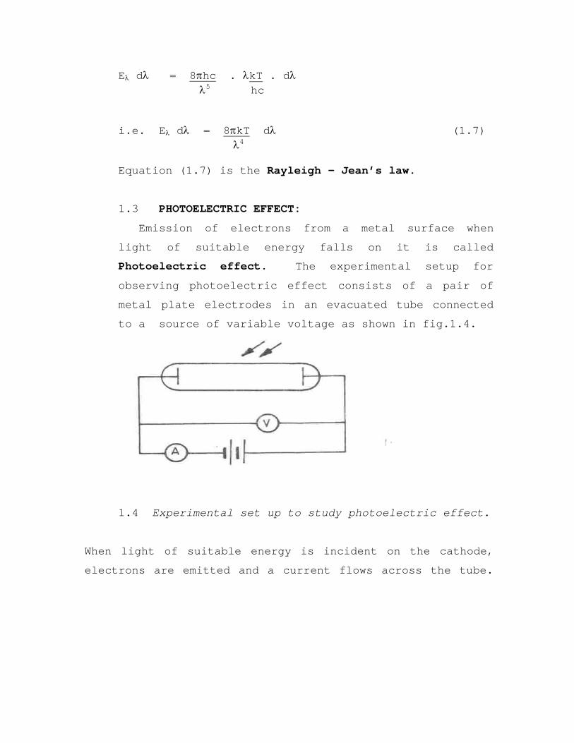
1.3 PHOTOELECTRIC EFFECT:

Emission of electrons from a metal surface when

light of suitable energy falls on it is called

Photoelectric effect. The experimental setup for

observing photoelectric effect consists of a pair of

metal plate electrodes in an evacuated tube connected

to a source of variable voltage as shown in fig.1.4.

1.4 Experimental set up to study photoelectric effect.

When light of suitable energy is incident on the cathode,

electrons are emitted and a current flows across the tube.

The characteristic curves for the photoelectric emission as

shown in fig. 1.5.

1.5 Current – voltage characteristics of photocell. The Intensity of illumination increases from L1 to L3.

The important properties of the emission are as

follows:

(i) There is no time interval between the incidence of

light and the emission of photoelectrons.

(ii) There is a minimum frequency for the incident

light below which no photoelectron emission occurs.

This minimum frequency, called threshold frequency,

depends on the material of the emitter surface. The

energy corresponding to this threshold frequency is the

minimum energy required to release an electron from the

emitter surface. This energy is characteristic of the

material of the emitter and is called the work function

of the material of the emitter.

(iii) For a given constant frequency of incident

light, the number of photoelectrons emitted or the

photo current is directly proportional to the intensity

of incident light.

(iv) The photoelectron emission can be stopped by

applying a reverse voltage to the phototube, i.e. by

making the emitter electrode positive and the collector

negative. This reverse voltage is independent of the

intensity of incident radiation but increases with

increase in the frequency of incident light. The

negative collector potential required to stop the photo

electron emission is called the stopping potential.

These characteristics of photoelectron emission can

not be explained on the basis of classical theory of

light but can be explained using the quantum theory of

light. According to this theory, emission of electrons

from the metal surface occurs when the energy of the

incident photon is used to liberate the electrons from

their bound state. The threshold frequency corresponds

to the minimum energy required for the emission. This

minimum energy is called the work function of the

metal. When the incident photon carries an energy in

excess of the work function, the extra energy appears

as the kinetic energy of the emitted electron. When the

intensity of light increases, the number of

photoelectrons emitted also increases but their kinetic

energy remains unaltered. The reverse potential

required to stop the photoelectron emission, i.e. the

stopping potential, depends on the energy of the

incident photon and is numerically equivalent to the

maximum kinetic energy of the photoelectrons.

When a photon of frequency ν is incident on a metal

surface of work function Φ, then,

hν = Φ + (½ mv2)max (1.8)

where (½ mv2)max is the maximum kinetic energy of the

emitted photoelectrons. This is known as Einstein’s

photoelectric equation. Since Φ = hνo, it can also be

written as

(½ mv2)max = hν– Φ = h(ν-νo ) (1.9)

If Vo is the stopping potential corresponding to the

incident photon frequency ν, then,

(½ mv2)max = hν – Φ = eVo (1.10)

Then, by experimental determination of Vo, it is

possible to find out the work function of the metal.

The experimental observation of photoelectric

effect leads to the conclusion that the energy in light

is not spread out over wavefronts but is concentrated

in small packets called photons. All photons of a

particular frequency have the same energy. A change in

the intensity of the incident light will change the

number of photoelectrons emitted but not their

energies. Higher the frequency of the incident light,

higher will be the kinetic energy of the

photoelectrons. These observations confirm the particle

properties of light waves.

1.4 COMPTON EFFECT:

When x-rays are scattered by a solid medium, the

scattered x-rays will normally have the same frequency

or energy. This is a case of elastic scattering or

coherent scattering. However, Compton observed that in

addition to the scattered x-rays of same frequency,

there existed some scattered x-rays of a slightly

higher wavelength (i.e., lower frequency or lower

energy). This phenomenon in which the wavelength of x-

rays show an increase after scattering is called

Compton effect.

Compton explained the effect on the basis of the

quantum theory of radiation. Considering radiation to

be made up of photons, he applied the laws of

conservation of energy and momentum for the interaction

of photon with electron. Consider an x-ray photon of

energy hν incident on an electron at rest (fig. 1.6.)

After the interaction, the x-ray photon gets scattered

at an angle θ with its energy changed to a value hν’ and

the electron which was initially at rest recoils at an

angle Φ. It can be shown that the increase in

wavelength is given by

1.6 Schematic diagram of the scattering of a photon by

a stationary electron.

∆λ = _h_ moc

(1-cos θ) (1.11)

where mo is the rest mass of the electron.

When θ = 90o, ∆λ = __h__ moc

= 0.0242 A°.

This constant value is called Compton wavelength.

When θ = 180o, ∆λ = moc

2h

Experimental observation indicate that the change in

the wavelength of the scattered x-rays is indeed in

agreement with equation (1.11), thus providing further

confirmation to the photon model.

Thus, Planck’s theory of radiation, photoelectric

effect and Compton effect are experimental evidences in

favour of the quantum theory of radiation.

1.5 MATTER WAVES AND DE BROGLIE’S HYPOTHESIS

Quantum theory and the theory of relativity are the

two important concepts that led to the development of

modern physics. The quantum theory was first proposed

by Planck to explain and overcome the inadequacies of

classical theories of black body radiation. The

consequences were very spectacular. Louis de Broglie

made the suggestion that particles of matter, like

electrons, might possess wave properties and hence

exhibit dual nature. His hypothesis was based on the

following arguments:

The Planck’s theory of radiation suggests that energy

is quantized and is given by

E = hν (1.12)

where ν is the frequency associated with the radiation.

Einstein’s mass-energy relation states that

E = mc2 (1.13)

Combining the two equations, it can be written as

E = hν = mc2

Hence, the momentum associated with the photon is given

by

P = mc = hν/c = h/λ

Extending this to particles, he suggested that any

particle having a momentum p is associated with a wave

of wavelength λ given by

λ = h/p (1.14)

This is called de Broglie’s hypothesis of matter waves

and λ is called the de Broglie wavelength.

The de Broglie wavelength can be calculated for any

particle using the above relation. In case of charged

particles like electrons, a beam of high energy

particles can be obtained by accelerating them in an

electric field. For example, an electron starting from

rest when accelerated with a potential difference V,

the kinetic energy acquired by the electron is given by

(1/2)mv2 = eV

where v is the velocity of the electron. The momentum

may be calculated as

p = mv = (2meV)1/2

Using the de Broglie equation, the wavelength

associated with the accelerated electron can be

calculated as

λ = h/p = h/(2meV)1/2 (1.15)

This equation suggests that, at a given speed, the de

Broglie wavelength associated with the particle varies

inversely as the mass of the particle. This concept of

matter waves aroused great interest and several

physicists launched experiments designed to test the

hypothesis. Heisenberg and Schrodinger proceeded on to

develop mathematical theories whereas Davisson and

Germer, G.P.Thomson and Kikuchi attempted experimental

verification.

1.5.1 Davisson-Germer experiment The hypothesis of de Broglie was verified by the

electron diffraction experiment conducted by Davisson

and Germer in the United States. The experimental set

up used by them is shown in the figure 1.7.

1.7 Experimental arrangement for Davisson-Germer

experiment.

The apparatus consists of a filament heated with a

small a.c power supply to produce thermionic emission

of electrons. These electrons are attracted towards an

anode in the form of a cylinder with a small aperture

maintained at a finite positive potential with respect

to the filament. They pass through the narrow aperture

forming a fine beam of accelerated electrons. This

electron beam was made to incident on a single

crystalline sample of nickel. The electrons scattered

at different angles were counted using an ionization

counter as a detector. The experiment was repeated by

recording the scattered electron intensities at various

positions of the detector for different accelerating

potentials (Fig.1.8).

Fig.1.8. Scattered electron intensity maps at different

accelerating potentials.The vertical axis represents

the direction of the incident electron beam and ф is

the scattering angle.The radial distance from the

origin at any angle represents the intensity of

scattered electrons.

When a beam of electrons accelerated with a potential

of 54 V was directed perpendicular to the nickel

target, a sharp maximum occurred in the electron

density at an angle of 500 with the incident beam. When

the angle ф between the direction of the incident beam

and the direction of the scattered beam is 500, the

angle of incidence will be 250 and the corresponding

angle of diffraction θ will be 650. The spacing of the

planes responsible for diffraction was found to be

0.091 nm from x-ray diffraction experiment. Assuming

first order diffraction, the wavelength of the electron

beam can be calculated as

λ = 2d sin θ = 2 x 0.091 x sin 650 = 0.165 nm.

The wavelength of the electrons can also be calculated

using the de Broglie’s relation as

λ = h/(2meV)1/2

= 6.63 x 10-34/(2 x 9.1 x 10-31 x 1.6 x 10-19 x 54)1/2

= 0.166 nm.

Thus, the Davisson-Germer experiment directly verifies

the de Broglie’s hypothesis.

1.5.2 G.P.Thomson experiment At almost the same time as the Davisson-Germer

experiment, G.P.Thomson of England carried out electron

diffraction experiments independently using a thin

polycrystalline foil of aluminium metal. The

experimental set up is shown in fig. 1.9.

1.9 Experimental arrangement of G.P.Thomson experiment.

He allowed a beam of accelerated electrons to fall on

the aluminium foil and observed a diffraction pattern

consisting of a series of concentric rings around the

direction of the incident beam. This pattern was

similar to the Debye-Scherrer pattern obtained for

aluminium using x-ray diffraction. Using the data

available on aluminium, he calculated the wavelength of

the electrons using the Bragg’s equation,

nλ = 2d sin θ

He also calculated the de Broglie wavelength of the

electrons with the knowledge of accelerating potential

using the relation,

λ = h/(2meV)1/2

The value of wavelength calculated from the two

equations matched well thereby experimentally proving

the de Broglie’s relation.

A similar experiment was conducted by Kikuchi in

Japan in which he obtained electron diffraction pattern

by passing an electron beam through a thin foil of mica

to confirm the validity of de Broglie’s relation.

The wave nature of particles is not restricted to

electrons. Any particle with a momentum p has a de

Broglie wavelength equal to (h/p). Neutrons produced in

nuclear reactors possess energies corresponding to

wavelength of the order of 0.1 nm. These particles also

should be suitable for diffraction by crystals.

Neutrons from a nuclear reactor are slowed down to

thermal energy of the order of kT and used for

diffraction and interference experiments. The results

agree well with the de Broglie relation. Since neutrons

are uncharged particles, they are particularly useful

in certain situations for diffraction studies. Neutron

beams have also been used as probes to investigate the

magnetic properties of nuclei.

1.5.3 Wave packet and de Broglie waves We have seen that moving particles may be

represented by de Broglie waves. The amplitude of these

de Broglie waves does not represent any parameter

directly describing the particle but is related to the

probability of finding the particle at a particular

place at a particular time. Hence, we cannot describe

de Broglie waves with a simple wave equation of the

type,

y = A cos(ωt-kx) (1.16)

Instead, we have to use an equation representing a

group of waves. In other words, a wave packet

consisting of waves of slightly differing wavelengths

may represent the moving particle. Superposition of

these waves constituting the wave packet results in the

net amplitude being modified, thereby defining the

shape of the wave group. The phase velocity of

individual waves depends on the wavelength. Since the

wave group consists of waves with different

wavelengths, all the waves do not proceed together and

the wave group has a velocity different from the phase

velocities of the individual waves. Hence, de Broglie

waves may be associated with group velocity rather than

the phase velocity.

1.5.4 Characteristics of matter waves 1. Matter waves are associated with a moving body.

2. The wavelength of matter waves is inversely

proportional to the velocity with which the body

is moving. Hence, a body at rest has an infinite

wavelength and the one traveling with a high

velocity has a lower wavelength.

3. Wavelength of matter waves also depends on the

mass of the body and decreases with increase in

mass. Due to this reason, the wavelike behaviour

of heavier bodies is not very evident whereas wave

nature of subatomic bodies could be observed

experimentally.

4. A wave is normally associated with some quantity

that varies periodically with the frequency of the

wave. For example, in a water wave, it is the

height of the water surface; in a sound wave it is

the pressure and in an electromagnetic wave, it is

the electric and magnetic fields that vary

periodically. But in matter waves, there is no

physical quantity that varies periodically. We use

a wave function to define matter waves and this

wave function is related to the probability of

finding the particle at any place at any instant,

which varies periodically.

5. Matter waves are represented by a wave packet made

up of a group of waves of slightly differing

wavelengths. Hence, we talk of group velocity of

matter waves rather than the phase velocity. The

group velocity can be shown to be equal to the

particle velocity.

6. Matter waves show properties similar to other

waves. For example, a beam of accelerated

electrons produces interference and diffraction

effects similar to an electromagnetic wave of

same wavelength.

1.6 PHASE AND GROUP VELOCITIES:

A wave is represented by the formula

y = A cos (ωt – kx) (1.16)

where y is the displacement at any instant t, A is the

amplitude of vibration, ω is the angular frequency

equal to 2πν and k is the wave vector, equal to (2π/λ).

The phase velocity of such a wave is the velocity with

which a particular phase point of the wave travels.

This corresponds to the phase being constant.

i.e., (ωt – kx) = constant

or x = constant + ωt/k

Phase velocity vp = dx/dt = ω/k

= 2πν/(2π/λ) = λν (1.17)

vp is called the ‘wave velocity’ or ‘phase velocity’.

The de Broglie waves are represented by a wave packet

and hence we have ‘group velocity’ associated with

them. Group velocity is the velocity with which the

wave packet travels. In order to understand the concept

of group velocity, consider the combination of two

waves represented by the formula

y1 = A cos (ωt-kx)

y2 = A cos {(ω+∆ω)t – (k+∆k)x }

The resultant displacement is given by

y = y1 + y2 = 2A cos {(ω+ω+∆ω)t–(k+k+∆k)x} cos 2 2

(∆ωt-∆kx)

≈ 2A cos(ωt–kx).cos(∆ωt/2-∆kx/2) (1.18)

The velocity of the resultant wave is given by

the speed with which a reference point, say the maximum

amplitude point, moves. Taking the amplitude of the

resultant wave as constant, we have

2A cos(∆ωt/2-∆kx/2) = constant

or (∆ωt/2-∆kx/2) = constant

or x = constant + (∆ωt/∆k)

Group velocity vg = dx/dt = (∆ω/∆k) (1.19)

Instead of two discrete values for ω and k,

if the group of waves has a continuous spread from ω to

(ω+∆ω) and k to (k+∆k), then, the group velocity is

given by

vg = dω (1.20) dk

It can be shown that the group velocity of the wave

packet is equal to the velocity of the particle with

which the wave packet is associated.

1.6.1 Relation between phase velocity and group

velocity:

We have the mathematical relation for phase velocity

given by

vp = ω/k or ω = k.vp

The group velocity vg is given by

vg = dω dk dk

= d(k.vp)

= vp + k.dvp dk

= vp + (2π/λ). dvp d(2π/λ)

= vp + (2π/λ).(-λ2/2π). dλ

dvp

= vp - λ. dvp dλ

(1.21)

In the above expression, if (dvp/dλ) = 0, i.e., if the

phase velocity does not depend on wavelength, then the

group velocity and phase velocity are equal. Such a

medium is called a non-dispersive medium. In a

dispersive medium, (dvp/dλ) is positive and hence the

group velocity is less than the phase velocity.

1.6.2 Relation between group velocity and particle

velocity (Velocity of de Broglie waves):

The phase velocity of waves depend on the

wavelength. This is responsible for the well known

phenomenon of dispersion. In the case of light waves in

vacuum, the phase velocity is same for all wavelengths.

In the case of de Broglie waves, we have,

ω = 2πν = 2πmc2/h = 2πm0c2 h(1-v2/c2)1/2

(1.22)

and k = 2π/λ = 2πmv/h = 2πm0v h(1-v2/c2)1/2

(1.23)

The group velocity of de Broglie waves is given by

Vg = dω/dk = dω/dv dk/dv

dω/dv = (2πm0c2/h).d(1-v2/c2)1/2 = 2πm0v dv h(1-v2/c2)3/2

(1.24)

dk/dv = ____2πm0__ h(1-v2/c2)3/2

___ (1.25)

From equations 1.24 and 1.25 we get,

vg = v

Thus, the group velocity associated with de

Broglie waves is just equal to the velocity with which

the particle is moving. If we try to calculate the

phase velocity,

Vp= ω/k = c2/v = c2/vg (1.26)

Since the group velocity or the particle velocity is

always less than c, the phase velocity of de Broglie

waves turn out to be greater than c. This only

indicates that we cannot talk of phase velocity of de

Broglie waves since they are made up of a group of

waves. Phase velocity has no physical significance for

de Broglie waves.

1.6.3 Derivation of de Broglie relation: The de Broglie relation may be derived as follows.

If we assume a particle having a kinetic energy equal

to mv2/2 to have a de Broglie wavelength λ, we can

write

hν = mv2/2 (assuming the energy of the particle

to be purely kinetic)

or ν = _m .v2 (1.27) 2h Differentiating with respect to λ,

dν = m . 2v. dv dλ 2h dλ

(1.28)

But we have vg = v = dω = 2πdν = -λ2

dk 2πd(1/λ) dλ dν

∴ dν = - v_ dλ λ2

(1.29)

Substituting in eqn.1.28, we get mv . dv h dλ λ2

= - v

Rewriting this, we have dv dλ mλ2

_ = - h_ (1.30)

Integrating with respect to λ,

v = h _ mλ

+ c

where c is the constant of integration. By applying the boundary condition that the wavelength tends to infinity as the velocity tends to zero, we find that the constant of integration has to be zero. Hence, we get

λ = _h_ (1.31) mv which is the de Broglie relation.

1.7 HEISENBERG’S UNCERTAINTY PRINCIPLE:

1.7.1 Origin and nature of the Principle:

When we assign wave properties to particles there

is a limitation to the accuracy with which we can

measure the properties like position and momentum.

1.10 A wave packet with an extension ∆x along x-axis.

Consider a wave packet as shown in fig.1.10. The

particle to which this wave packet corresponds to may

be located anywhere within the wave packet at any

instant. The probability density suggests that it is

most likely to be found in the middle of the wave

packet. However, there is a finite probability of

finding the particle anywhere within the wave packet.

If the wave packet is smaller in extension, the

position of the particle can be specified more

precisely. But the wavelength of the waves will not be

well defined in a narrow wave packet. Since wavelength

is related to momentum through de Broglie’s relation,

the momentum is not precisely known. On the otherhand,

a wave packet with large extension can have a more

clearly defined wavelength and hence momentum at the

cost of the knowledge about the position. This leads

to the conclusion that it is impossible to know both

the position and momentum of an object precisely at the

same time. This is known as Uncertainty principle.

For a wave packet of extension ∆x with an

uncertainty in the wave number ∆k assuming the

uncertainties to be the standard deviation in the

respective quantities, it may be shown that a minimum

value of the product of such deviations is given by

∆x . ∆k = ½ (1.32)

This minimum value of the product of uncertainties is

for the case of a gaussian distribution of the wave

functions. Since the wave packets in general do not

have gaussian forms, the uncertainty relation becomes

∆x . ∆k ≥ ½ (1.33)

But we have

k = 2π/λ (1.34)

Also λ = h/p (1.35)

Hence, k = 2πp/h

∆k = 2π

. ∆p (1.36) h

Substituting in equation (1.33), we get

∆x . ∆p ≥ h_ 4π

or ∆x. ∆p ≥ ħ (1.37) 2

This equation states that the product of

uncertainty ∆x in the position of an object at some

instant and the uncertainty in the momentum in the x-

direction at the same instant is equal to or greater

than ħ/2.

Another form of uncertainty principle relates

energy and time. In the atomic process, if energy E is

emitted as an electromagnetic wave during an interval

of time ∆t, then, the uncertainty ∆E in the measured

value of E depends on the duration of the time interval

∆t according to the equation,

∆E . ∆t ≥ ħ/2 (1.38)

It may be mentioned that these uncertainties

are not due to the limitations of the precision of the

measuring methods or measuring instruments but due to

the nature of the quantities involved.

1.7.2 An illustration of uncertainty principle:

We have the following ‘Thought experiment’ to

illustrate the uncertainty principle. Imagine an

electron being observed using a microscope (fig.1.11).

1.11 Schematic diagram of experimental set up to study uncertainty principle.

The process of observation involves a photon of

wavelength λ incident on the electron and getting

scattered into the microscope. The event may be

considered as a two-body problem in which a photon

interacts with an electron. The change in the velocity

of the photon during the interaction may be anything

between zero( for grazing angle of incidence) and 2c

( for head-on collision and reflection). The average

change in the momentum of the photon may be written as

equal to (hν/c) or (h/λ). This difference in momentum

is carried by the recoiling electron which was

initially at rest. The change or uncertainty in the

momentum of the electron may thus be written as (h/λ).

At the same time, the position of the electron can be

determined to an accuracy limited by the resolving

power of the microscope, which is of the order of λ.

Hence, the product of the uncertainties in position and

momentum is of the order of h. This argument implies

that the uncertainties are associated with the

measuring process. This illustration only estimates

the accuracy of measurement, the uncertainty being

inherent in the nature of the moving particles

involved.

1.7.3 Physical significance of uncertainty principle:

Uncertainty principle is a consequence of the wave

particle duality. It states that it is impossible to

know both the position and momentum of an object

exactly and at the same time. Mathematically, it can

be shown that the product of uncertainties in the

position and momentum measured simultaneously will have

a value greater than ħ/2, ie (h/4π). If ∆x is the

uncertainty in the measurement of the position x of an

object and ∆px is the uncertainty in the measurement

of momentum px , then, at any instant,

∆x . ∆px > ħ/2

We can try to estimate the product of the uncertainties

with the help of illustrations as the one mentioned

above. The principle is based on the assumption that a

moving particle is associated with a wave packet, the

extension of which in space accounts for the

uncertainty in the position of the particle. The

uncertainty in the momentum arises due to the

indeterminacy of the wavelength because of the finite

size of the wave packet. Thus, the uncertainty

principle is not due to the limited accuracy of

measurement but due to the inherent uncertainties in

determining the quantities involved. But we can still

define the position where the probability of finding

the particle is maximum and also the most probable

momentum of the particle.

1.7.4 Applications of uncertainty principle:

The uncertainty principle has far reaching

implications. In fact, it has been very useful in

explaining many observations which cannot be explained

otherwise. A few of the applications of the uncertainty

principle are worth mentioning.

(a) Diffraction of a beam of electrons: Diffraction of

a beam of electrons at a slit is the effect of

uncertainty principle. As the slit is made narrower,

thereby reducing the uncertainty in the position of the

electrons in the beam, the beam spreads even more

indicating a larger uncertainty in its velocity or

momentum.

1.12 Diffraction at a single slit.

Figure 1.12 shows the diffraction of an electron beam

by a narrow slit of width ∆x. The beam traveling along

OX is diffracted along OY through an angle θ. Due to

the wave nature of the electron, we observe Fraunhoffer

diffraction on the screen placed along XY. The accuracy

with which the position of the electron is known is ∆x

since it is uncertain from which place in the slit the

electron passes. According to the theory of

diffraction, we have

λ = ∆x.sin θ or ∆x = λ/ sin θ

Further, the initial momentum of the electron along XY

was zero and after diffraction, the momentum of the

electron is p. sin θ where p is the momentum of the

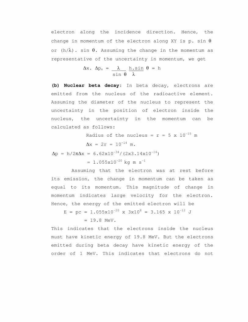
electron along the incidence direction. Hence, the

change in momentum of the electron along XY is p. sin θ

or (h/λ). sin θ. Assuming the change in the momentum as

representative of the uncertainty in momentum, we get

∆x. ∆px = λ h.sin sin θ λ

θ = h

(b) Nuclear beta decay: In beta decay, electrons are

emitted from the nucleus of the radioactive element.

Assuming the diameter of the nucleus to represent the

uncertainty in the position of electron inside the

nucleus, the uncertainty in the momentum can be

calculated as follows:

Radius of the nucleus = r = 5 x 10-15 m

∆x = 2r = 10-14 m.

∆p = h/2π∆x = 6.62x10-34/(2x3.14x10-14)

= 1.055x10-20 kg m s-1

Assuming that the electron was at rest before

its emission, the change in momentum can be taken as

equal to its momentum. This magnitude of change in

momentum indicates large velocity for the electron.

Hence, the energy of the emitted electron will be

E = pc = 1.055x10-20 x 3x108 = 3.165 x 10-12 J

= 19.8 MeV.

This indicates that the electrons inside the nucleus

must have kinetic energy of 19.8 MeV. But the electrons

emitted during beta decay have kinetic energy of the

order of 1 MeV. This indicates that electrons do not

exist in the nucleus of the atom but are ‘manufactured’

by the nucleus at the time of decay.

(c)Binding energy of an electron in an atom: In a

hydrogen atom, the electron revolves round the nucleus

in an orbit of radius 5 X 10-11 m. Assuming this as the

maximum uncertainty in position, we can calculate

the minimum uncertainty in the momentum as

(∆p)min = h/2π(∆x)max = 2.1 X 10-24 kg m s-1.

Assuming this as the momentum of electron, the kinetic

energy of the electron will be equal to

K.E. = p2/2m = 2.45 X 10-18 J = 15.3 eV.

Thus, the binding energy of an electron in hydrogen

atom is nearly 15 eV which is found to be correct

experimentally.

(d) Nitrogen doping of silicon: The laws of

conservation of energy and momentum restrict the

generation and recombination processes in

semiconductors. Silicon, which is an indirect band gap

semiconductor, has low efficiency as a material for

photo diode or light emitting diode. Nitrogen doping of

silicon will bind the free electrons to the lattice

thereby restricting the value of uncertainty in

position. This results in a larger uncertainty in

momentum thereby increasing the probability for

generation or recombination process.

1.8 WAVE MECHANICS:

Quantum theory is based on the quantization

of energies. It deals with the particle nature of

radiation. It implies that addition or liberation of

energy will be between discrete energy levels. It

assigns particle status to a packet of energy by

calling it ‘quantum of energy’ or ‘photon’ and treats

the interaction of radiation with matter as a two-body

problem. On the other hand, de Broglie’s hypothesis and

the concept of matter waves led to the development of a

different formulation called ‘Wave mechanics’. This

deals with the wave properties of material particles.

It was shown later that the quantum mechanics and the

wave mechanics are mathematically identical and lead to

the same conclusion.

1.8.1 Characteristics of wave function:

Waves in general are associated with quantities

that vary periodically. For example, water waves

involve the periodic variation of the height of the

water surface at a point. Similarly, sound waves are

associated with periodic variations of the pressure.

In the case of matter waves, the quantity that varies

periodically is called ‘wave function’. The wave

function, represented by ψ, associated with matter

waves has no direct physical significance. It is not

an observable quantity. But the value of the wave

function is related to the probability of finding the

body at a given place at a given time. The square of

the absolute magnitude of the wave function of a body

evaluated at a particular time at a particular place is

proportional to the probability of finding the body at

that place at that instant.

The wave functions are usually complex. The

probability in such a case is taken as ψ∗ψ, i.e. the

product of the wave function with its complex

conjugate. Since the probability of finding the body

somewhere is finite, we have the total probability over

all space equal to certainty.

i.e.∫ ψ∗ψ dV = 1 (1.39)

Equation (1.39) is called the normalization condition

and a wave function that obeys the equation is said to

be normalized. Further, ψ must be single valued since

the probability can have only one value at a particular

place and time. Since the probability can have any

value between zero and one, the wave function must be

continuous. Momentum being related to the space

derivatives of the wave function, the partial

derivatives ∂ψ/∂x, ∂ψ/∂y and ∂ψ/∂z must also be

continuous and single valued everywhere. Thus, the

important characteristics of wave function are as

follows:

(1) ψ must be finite, continuous and single valued

everywhere.

(2) ∂ψ/∂x, ∂ψ/∂y and ∂ψ/∂z must be finite, continuous

and single valued everywhere.

(3) ψ must be normalizable.

1.8.2 Physical significance of wave function:

We have already seen that the wave function has no

direct physical significance. However, it contains

information about the system it represents and this can

be extracted by appropriate methods. Even though the

wave function itself is not directly an observable

quantity, the square of the absolute value of the wave

function is intimately related to the moving body and

is known as the probability density. This probability

density is the quantum mechanical method of finding the

body at a particular position at a particular time. The

wave function carries information about the particle’s

wave-like behaviour. It also provides information about

the momentum and energy of the particle at any instant

of time.

1.8.3 Schrodinger’s wave equation:

The motion of a free particle can be described

by the wave equation.

ψ = A exp{-i(ωt –kx)} (1.40)

But ω = 2 πν = 2π (E/h) = (E/ħ) and k = 2π/λ = 2π (p/h) = (p/ħ) where E is the total energy and p is the momentum of

the particle. Substituting in the equation (1.40), we

get,

ψ = A exp{-i ħ

(Et-px)} (1.41)

Differentiating equation (1.41) with respect to

x twice, we get,

∂2ψ = -p2 ψ or p2ψ = - ħ2 . ∂2ψ ∂x2 ħ2 ∂x2

(1.42)

Differentiating equation (1.41) with respect to t, we get, ∂ψ = - iE . ψ or E ψ = - ħ . ∂ψ ∂t ħ i ∂t

(1.43)

The total energy of the particle can be written as

E = p2

2m + U (1.44)

where U is the potential energy of the particle.

Multiplying both sides of the equation by ψ

E ψ = p2

2m ψ + Uψ (1.45)

Substituting for Eψ and p2ψ from equation (1.42) and (1.43) - ħ ∂ψ = - ħ2 ∂2ψ i ∂t 2m ∂x2

+ Uψ (1.46)

This is known as Schrodinger’s time dependent equation

in one dimension.

The wave function ψ in equation (1.41) may also be

written as

ψ = A exp{-i (Et-px)} = A exp(-iEt) . exp(ipx ħ ħ ħ

)

ψ = Φ exp (-iEt ħ

) (1.47 )

where Φ is a position dependent function. Substituting

this form of ψ in equation (1.45),

EΦ exp(-iEt) = p2 Φ exp(-iEt) + UΦ exp(-iEt ħ 2m ħ ħ

)

or EΦ exp(-iEt) = - ħ2 . ∂2Φ . exp(-iEt) + UΦ exp(-iEt ħ 2m ∂x2 ħ ħ

)

or ∂2Φ exp(-iEt) + 2m (E-U)Φ exp(-iEt ∂x2 ħ ħ2 ħ

) = 0

or ∂2ψ + 2m ∂x2 ħ2

(E-U)ψ = 0 (1.48)

This is the Schrodinger’s wave equation in one

dimension. In three dimensions, the above equation may

be written as

∂2ψ + ∂2ψ + ∂2ψ + 2m(

E-U)ψ = 0 ∂x2 ∂y2 ∂z2 ħ2

or ∇2ψ + 2m( ħ2

E-U)ψ =0

This equation is known as the steady state or time

independent Schrodinger wave equation in three

dimensions.

1.8.4 Eigen values and eigen functions:

These terms come from the German words and mean

proper or characteristic values or functions

respectively. The values of energy for which the

Schrodinger’s equation can be solved are called ‘Eigen

values’ and the corresponding wave functions are called

‘Eigen functions’. The eigen functions possess all the

characteristics properties of wave functions in

general (see section 1.8.1).

1.9 APPLICATIONS OF SCHRODINGER’S EQUATION:

1.9.1 Case of a free particle: A free particle is defined as one which is not

acted upon by any external force that modifies its

motion. Hence, the potential energy U in the

Schrodinger’s equation is a constant and does not

depend on position or time. For convenience, the

potential energy may be assumed to be zero. Then, the

Schrodinger’s equation for the particle becomes

∂2ψ + 2m ∂x2 ħ2

Eψ = 0 (1.49)

where E is the total energy of the particle which is

purely kinetic. This is of the form,

∂2ψ ∂x2

+ k2ψ = 0

where k2 = 2mE/ħ2. The solution of this equation may be

written as

ψ = A cos kx + B sin kx

Solving for the constants A and B pose some

difficulties because we cannot apply any boundary

conditions on the wave function as it represents a

single wave which is not localized and not

normalizable. Since the solution has not imposed any

restriction on the value of k, the free particle is

permitted to have any value of energy given by the

equation,

E = ħ2k2/2m

Since the total energy is purely kinetic, the momentum

of the particle would be p = ħk or h/λ. This is just

what we would expect, since we have constructed the

Schrodinger equation to yield the solution for the free

particle corresponding to a de Broglie wave.

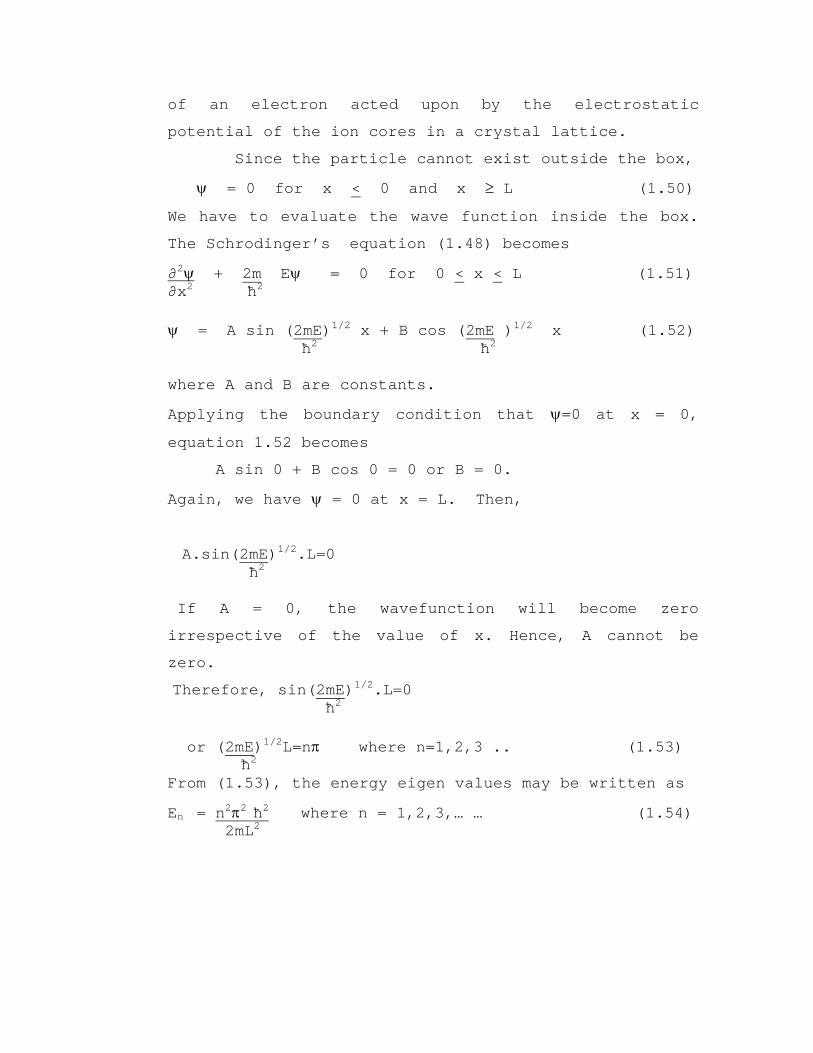
1.9.2 Particle in a box:

The simplest problem for which Schrodinger’s

time independent equation can be applied and solved is

the case of a particle trapped in a box with

impenetrable walls.

Consider a particle of mass m and energy E

travelling along x-axis inside a box of width L. The

particle is thus restricted to move inside the box by

reflections at x=0 and x=L (Fig. 1.13).

1.13 Schematic for a particle in a box. The height of the wall extends to infinity.

The particle does not lose any energy when it collides

with the walls and hence the total energy of the

particle remains constant. The potential energy of the

particle is considered to be zero inside the box and

infinite outside. Since the total energy of the

particle cannot be infinite, it is restricted to move

within the box. The example is an oversimplified case

of an electron acted upon by the electrostatic

potential of the ion cores in a crystal lattice.

Since the particle cannot exist outside the box,

ψ = 0 for x < 0 and x ≥ L (1.50)

We have to evaluate the wave function inside the box.

The Schrodinger’s equation (1.48) becomes

∂2ψ + 2m∂x2 ħ2

Eψ = 0 for 0 < x < L (1.51)

ψ = A sin (2mE)1/2 x + B cos (2mE ħ2 ħ2

)1/2 x (1.52)

where A and B are constants.

Applying the boundary condition that ψ=0 at x = 0,

equation 1.52 becomes

A sin 0 + B cos 0 = 0 or B = 0.

Again, we have ψ = 0 at x = L. Then,

A.sin(2mE ħ2

)1/2.L=0

If A = 0, the wavefunction will become zero

irrespective of the value of x. Hence, A cannot be

zero.

Therefore, sin(2mE ħ2

)1/2.L=0

or (2mE ħ2

)1/2L=nπ where n=1,2,3 .. (1.53)

From (1.53), the energy eigen values may be written as

En = n2π2 ħ2

2mL2 where n = 1,2,3,… … (1.54)

From this equation, we infer that the energy of the

particle is discrete as n can have integer values. In

other words, the energy is quantized. We also note that

n cannot be zero because in that case, the wave

function as well as the probability of finding the

particle becomes zero for all values of x. Hence, n = 0

is forbidden. The lowest energy the particle can

possess is corresponding to n = 1 and is equal to

E1 = π2ħ2

2mL2

This is called ‘ground state energy’ or ‘zero point

energy’. The higher excited states will have energies

like 4E1, 9E1, 16E1, etc. This indicates that the energy

levels are not equally spaced.

The wave functions or the eigen functions are

given by

ψn = A. Sin 2mEn ħ2

1/2 x

or ψn = A. Sin nπ L

x (1.55)

Applying the normalization condition,

i.e. ∫ A2 Sin2 nπx L

. dx = 1 (1.56)

Since the wave function is non-vanishing only for

0 < x < L, it can be shown that

∫ Sin2 nπx L 2

dx = (L ) (1.57)

Substituting in equation (1.56), we have A2 (L 2 L

) = 1 or A = ( 2 )1/2 (1.58)

The eigen function or wave functions in equation (1.55) becomes ψn = ( 2 )½ sin (2mEn L ħ2

)½ x

ψn = ( 2 )½ sin nπx L L

(1.59)

1.14 Variation of wave function associated with an electron confined to a box in its ground state & excited states.

Fig. 1.14 shows the variation of the wave function

inside the box for different values of n and Fig.1.15

shows the probability densities of finding the particle

1.15 Probability function as a function of position.

at different places inside the box for different

values of n. Thus, wave mechanics suggests that the

probability of finding any particle at the lowest

energy level is maximum at the centre of the box which

is in agreement with the classical picture. However,

the probability of finding the particle in higher

energy states is predicted differently by the two

formulations.

1.9.3 Finite Potential well: In real life situations, the potential energy is

never infinite. The box with impenetrable walls has no

physical significance. However, we come across

situations where the potential energy is finite. Let us

try to solve the case of an electron in a finite

potential well. We can consider two different cases

corresponding to the following situations:

(i) the total energy E being greater than the

potential energy U, and

(ii) the total energy E being less than the

potential energy U.

Fig 1.16 Schematic for a particle in a potential well of finite depth ( E greater than U).

The first case may be represented by the figure

1.16. Consider the particle with total energy E inside

a potential well of height U. In the region II, where

the particle is not influenced by the potential (U =

0), the solution of the Schrodinger’s equation is of

the form,

ψ = A cos kx + B sin kx

where k = (2mE/ħ2)1/2. This particle may be represented

by a wave of wavelength λ = 2π/k. When the particle is

in region I and III, its wavelength changes to λ’=

2π/k’ where k’ = [2m(E-U)/ħ2]1/2. In other words, the

effect of the potential energy step is to reduce the

kinetic energy of the particle as evident from an

increase in the value of the wavelength.

In the second case, the total energy of the

particle is less than the potential energy. Under this

condition, classically, the particle cannot propagate

beyond the step since this amounts to the kinetic

energy being negative. But, wave mechanically, a

different solution results. Let U be greater than the

total energy E of the electron but finite. To analyze

this case, we have to consider the three regions

separately.

In region II, since U = 0, the electron is free and the

Schrodinger’s equation is

d2ψ + 2m dx2 ħ2

Eψ = 0 (1.60)

In regions I and III, we have

d2ψ + 2m dx2 ħ2

(E – U) ψ = 0 (1.61)

The solutions for these equations can be assumed to be ψI = A ei

βx + B e-iβx in region I (1.62) ψII = C ei

αx + D e-iαx in region II (1.63)

and ψIII = F eiβx + G e-iβx in region III (1.64)

where α = [(2mE)/ħ2 ]1/2 (1.65)

β = [ 2m (E-U)/ħ2 ]1/2 (1.66)

since E is less than U, (E-U) is (-)ve and β is

imaginary.

Let us define a new constant

ϒ = -iβ (1.67)

Then the equations (1.62) and (1.64) become

ψI = A e-ϒx + B eϒx (1.68)

ψIII = F e-ϒx + G eϒx (1.69)

To evaluate the constants, we consider the boundary

condition in the region I where the wave function

should reduce to zero as x → -∞. Then eqn (1.68)

becomes

0 = A . ∞ + B .0 or A = 0.

∴ψI = B eϒx (1.70)

Similarly, in region III, since the wave function

should reduce to zero as x → ∞, eqn (1.69) becomes

0 = F . 0 + G . ∞ or G = 0.

∴ψIII = F e-ϒx (1.71)

This indicates that the wave function decreases

exponentially as we move away from the potential well

on either sides. Inside the potential well the wave

function represented by the equation (1.63) varies

sinusoidally. Further, since the wave function and its

derivative are continuous at the boundaries

corresponding to x = 0 and x = L, the wave functions

are non-zero at these boundaries. The plots of the wave

functions and the probability densities are shown in

Fig. 1.17 and 1.18 respectively.

1.17 Variation of wave function of a particle in a

finite potential well.

1.18 Probability function as a function of position.

Thus, we observe that in case of a particle in a

potential well of finite height, the particle has a

finite probability of penetrating into the wall.

However, if the walls of the well are infinitely thick,

the particle will be confined to the well and performs

oscillatory motion inside the well.

1.9.4 Tunnel effect: In the previous case of a finite potential well,

even though the height of the wall was finite, the

thickness of the wall was assumed to be infinite. As a

result, the particle was trapped in the well in spite

of penetrating into the wall. Under the same condition

of the total energy being less than the potential

energy, if the thickness of the wall is reduced and

made finite, the solution of the Schrodinger’s equation

predicts a finite probability of the particle passing

through the barrier and finding itself on the other

side. Thus, a particle without the necessary energy to

pass over the barrier can still penetrate through the

barrier. This phenomenon is called “Quantum mechanical

tunneling”.

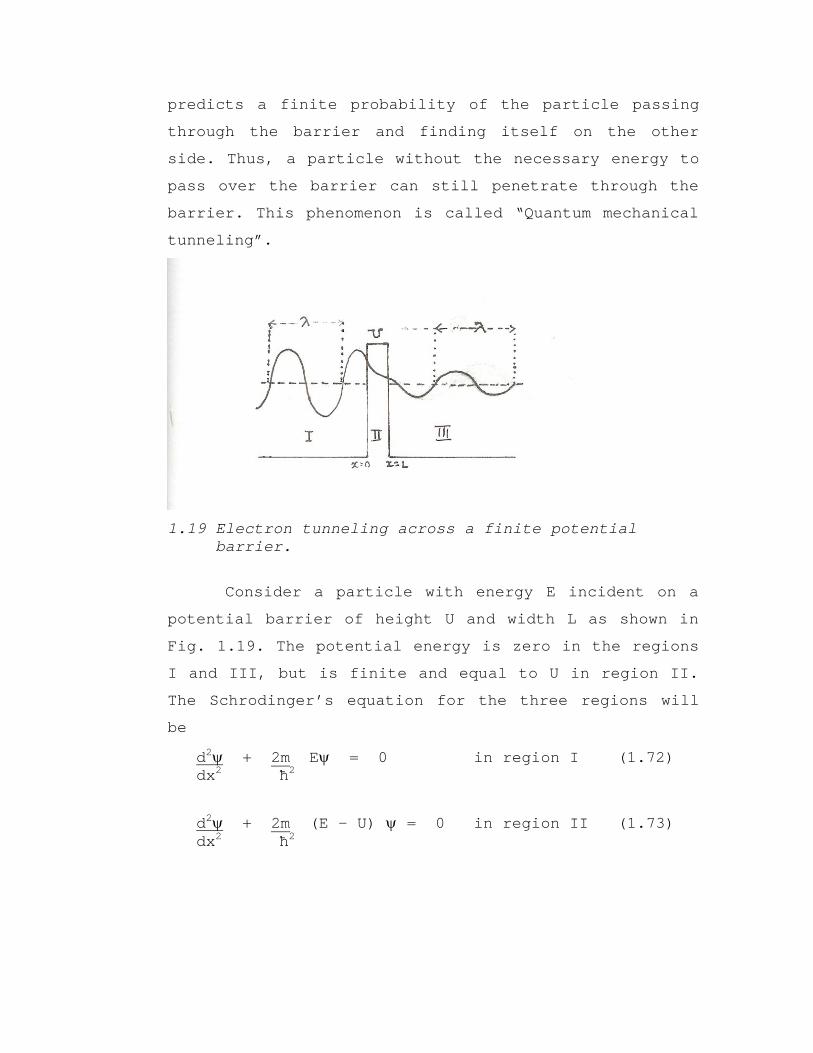
1.19 Electron tunneling across a finite potential barrier.

Consider a particle with energy E incident on a

potential barrier of height U and width L as shown in

Fig. 1.19. The potential energy is zero in the regions

I and III, but is finite and equal to U in region II.

The Schrodinger’s equation for the three regions will

be

d2ψ + 2m dx2 ħ2

Eψ = 0 in region I (1.72)

d2ψ + 2m dx2 ħ2

(E – U) ψ = 0 in region II (1.73)

d2ψ + 2m dx2 ħ2

Eψ = 0 in region III (1.74)

The solutions of these equations can be written as ψI = A ei

αx + B e-iαx in region I (1.75)

ψII = C e-ϒx + D eϒx in region II (1.76)

ψIII = F eiαx + G e-iαx in region III (1.77)

where α = [(2mE)/ħ2 ]1/2 (1.65)

β = [ 2m (E-U)/ħ2 ]1/2 (1.66)

and ϒ = -iβ (1.67)

The wavefunction in the region I is made up of two

terms as evident from Equation (1.75). The first term

with a positive exponent represents an incoming or

incident wave moving in the positive x-direction and

the second term represents a wave reflected by the

barrier moving in the negative x-direction. Similarly,

the first term in equation (1.77) represents the

transmitted wave moving in region III in the positive

x-direction. The wavefunction in the region II is given

by equation (1.76). Here, the exponents are real

quantities and hence the wavefunction does not

oscillate. The probability density ψII2 is finite and

represent the probability of finding the particle

within the barrier. Such a particle may emerge into

region III. This is called tunneling.

The transmission probability T for a particle to

pass through the barrier is given by

T = ψIII2 = FF ψI2 AA*

* ≅ e-2γL (1.78)

The above equation represents the dependence of

tunneling probability on the width of the barrier and

the energy of the particle.

1.9.5 Examples of tunneling across a finite barrier: There are a few examples of tunneling across a

thin finite potential barrier in nature. These

observations are in fact proof in favour of the theory

of quantum mechanical tunneling. Let us consider a few

of them.

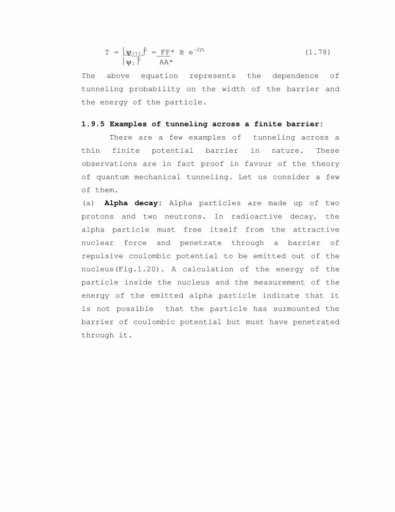
(a) Alpha decay: Alpha particles are made up of two

protons and two neutrons. In radioactive decay, the

alpha particle must free itself from the attractive

nuclear force and penetrate through a barrier of

repulsive coulombic potential to be emitted out of the

nucleus(Fig.1.20). A calculation of the energy of the

particle inside the nucleus and the measurement of the

energy of the emitted alpha particle indicate that it

is not possible that the particle has surmounted the

barrier of coulombic potential but must have penetrated

through it.

1.20 Emission of an α particle in nuclear decay.

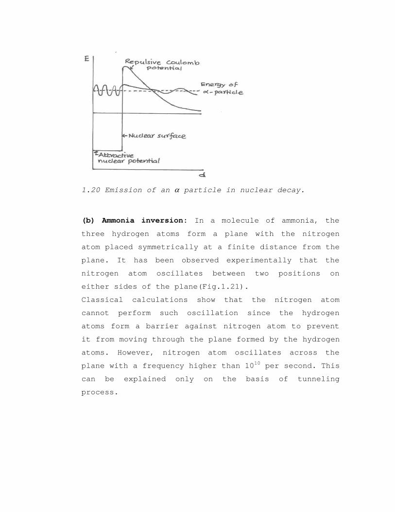
(b) Ammonia inversion: In a molecule of ammonia, the

three hydrogen atoms form a plane with the nitrogen

atom placed symmetrically at a finite distance from the

plane. It has been observed experimentally that the

nitrogen atom oscillates between two positions on

either sides of the plane(Fig.1.21).

Classical calculations show that the nitrogen atom

cannot perform such oscillation since the hydrogen

atoms form a barrier against nitrogen atom to prevent

it from moving through the plane formed by the hydrogen

atoms. However, nitrogen atom oscillates across the

plane with a frequency higher than 1010 per second. This

can be explained only on the basis of tunneling

process.

1.21 Schematic diagram of ammonia molecule. Nitrogen atom oscillates between two symmetric positions across the repulsive plane of hydrogen atoms.

(c) Zener and tunnel diodes: These are diodes made out

of heavily doped semiconductors with special

characteristics. The current-voltage characteristics of

these diodes can be explained only on the basis of

quantum mechanical tunneling process. The high speed of

operation of these devices can be explained only as due

to tunneling since the movement of charge carriers is

otherwise by diffusion which is a very slow process.

The scanning tunneling microscope is another device

operating on the principle of tunneling.

(d) Frustrated total internal reflection: Figure 1.22

shows a beam of light reflected totally from the

surface of glass. If a second prism of glass is brought

close to the first, the beam appears through the second

glass prism indicating tunneling of light through the

surfaces of glass which were otherwise acting as

barriers.

1.22 Demonstration of frustrated total internal reflection.

1.9.6. Theoretical interpretation of tunneling:

Penetration of a particle into the forbidden

region of a step or a barrier can be explained

with the help of Heisenberg’s uncertainty

principle. To enter this region, the particle must

gain an energy of atleast (U-E) and to move in

this region, it must have an additional kinetic

energy, K. This is a violation of the principle of

conservation of energy for the particle. However,

according to the uncertainty relation, we may

write

ΔE. Δt ≈ ћ (1.79)

According to this, the conservation of energy does

not apply for a time duration Δt if the change in

energy is not greater than ΔE. If we presume that

the particle borrows an energy ΔE and returns the

borrowed energy within a time interval of Δt, the

observer will still believe that the energy is

conserved. The time interval within which the

extra energy must be returned is given by

Δt = ћ/ΔE = ћ/(U-E+K) (1.80)

The particle moves with a velocity v given by

v = (2K/m)1/2 (1.81)

If the particle travels a distance Δx into the

forbidden region and returns, then, the total

distance travelled is 2Δx and hence we can write

Δx = v.Δt/2

= (1.82)

As the kinetic energy K tends to zero, the value

of Δx also tends to zero since the velocity tends

to zero. Also, as K tends to infinity, Δx tends to

zero since it is the distance travelled in a time

interval Δt tending to zero. In between these

limits, there must be a maximum value of Δx

corresponding to a particular value of K.

Differentiating Δx with respect to K in equation

1.82, we can find the maximum value of Δx as

Δxmax = (1.83)

Or Δxmax = (1/2ϒ) (1.84)

From equation 1.78, the probability of finding the

particle at a distance Δxmax from the step is

T = e-2ϒΔxmax = e-1 (1.85)

Hence, we may define the maximum penetration

distance as the distance at which the transmission

probability is (1/e).

It may be mentioned that the particle is

never observed in the forbidden region. The

particles incident on the potential energy step

will be reflected back. Some are reflected at the

step itself where as others penetrate a finite

distance before returning. If the barrier width is

small, the particle will re-emerge on the other

side of the barrier. This phenomenon is known as

quantum mechanical tunneling.

1.9.7 Harmonic oscillator:

When a body vibrates about an equilibrium

position, the body is said to be executing harmonic

motion. We have many examples of such motion which we

come across, like the vibration in a spring that is

stretched and released, vibrations of atoms in a

crystal lattice, etc. Whenever a system is disturbed

from its equilibrium position, it can come back to its

original position only under the influence of a

restoring force. Hence, the presence of a restoring

force is a necessary condition for harmonic motion. The

system oscillates indefinitely if there is no loss of

energy.

A special case of harmonic motion is simple

harmonic motion. In simple harmonic motion, the

restoring force F acting on a particle of mass m is

linear. In other words, the restoring force is

proportional to the displacement x of the particle from

its equilibrium position and is in the opposite

direction.

i.e., F = -kx (1.86)

where k is called the force constant. The relation is

called Hooke’s law. From the second law of motion, we

have,

F = ma (1.87)

∴ -kx = m dt2

d2x

or d2x dt2 m

+ k.x = 0 (1.88)

This is the equation for the simple harmonic

oscillator. The solution of this equation may be

written as

x = A cos (ωt+φ) (1.89)

where ω = 2πν = (k/m)1/2 (1.90)

ν is called the frequency of the oscillator. φ is the

phase angle and depends on the value of x at t = 0. The

potential energy U corresponding to the restoring force

F may be calculated as equal to the work done in

bringing a particle from x = 0 to x = x against the

force.

i.e., U(x) = - F(x) dx = k x dx = kx2/2 (1.91)

A plot of the potential energy U as a function of

displacement x is a parabola as shown in fig. 1.23.

This indicates that an oscillator with energy E

1.23 Energy states in a one dimensional harmonic oscillator.

vibrates back and forth with an amplitude from –a to

+a. Classically, it appears that the oscillator can

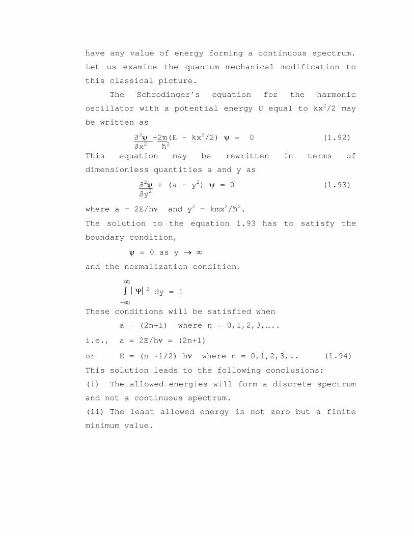
have any value of energy forming a continuous spectrum.

Let us examine the quantum mechanical modification to

this classical picture.

The Schrodinger’s equation for the harmonic

oscillator with a potential energy U equal to kx2/2 may

be written as

∂2ψ +2m ∂x2 ħ2

(E – kx2/2) ψ = 0 (1.92)

This equation may be rewritten in terms of

dimensionless quantities a and y as

∂2ψ ∂y2

+ (a – y2) ψ = 0 (1.93)

where a = 2E/hν and y2 = kmx2/ħ2.

The solution to the equation 1.93 has to satisfy the

boundary condition,

ψ = 0 as y → ∞

and the normalization condition,

∞ ∫ Ψ2 dy = 1 -∞ These conditions will be satisfied when

a = (2n+1) where n = 0,1,2,3,…..

i.e., a = 2E/hν = (2n+1)

or E = (n +1/2) hν where n = 0,1,2,3,.. (1.94)

This solution leads to the following conclusions:

(i) The allowed energies will form a discrete spectrum

and not a continuous spectrum.

(ii) The least allowed energy is not zero but a finite

minimum value.

At n = 0, E0 = hν/2

This minimum energy E0 is called the zero point

energy. It is also observed that the higher energy

levels are all equally spaced with a spacing of hν.

This is in contrast to the result obtained for the case

of a particle in a potential well of infinite depth.

1.9.8 Practical applications of Schrodinger’s wave

equation:

The real life situations are much different from

the one considered while deriving the Schrodinger’s

wave equation. This is especially true when one is

analyzing the motion of a particle like electron

traveling at velocities comparable to that of light.

Relativistic modification to the Schrodinger’s equation

and its solution are complex. Further, the boundary

condition of an infinitely high potential barrier is

never encountered. In case of metals, conduction

electrons move in crystal lattice under the influence

of finite potentials of the ion cores. The potential

energy due to the influence of external forces acting

on it may also be functions of position of the particle

and time. Incorporation of these factors while

formulating and solving the Schrodinger’s wave equation

has led to accurate prediction of the behaviour of

subatomic, atomic, molecular and other microscopic

systems.

NUMERICAL EXAMPLES:

1.1 Calculate the velocity of photoelectrons emitted

from a metal surface of work function 1.5 eV when the

metal surface is irradiated with a light beam of

wavelength 4 x 10-7 m.

Solution:

Incident energy = hν = hc = 6.62x10-34x3x108

λ 4 x 10-7

= 4.97x10-19 J

Threshold energy = hνo = Φ = 1.5eV = 1.5 x 1.6 x 10-19 J

= 2.4 x 10-19 J

Kinetic energy of electrons = (hν - hν0 )

= (4.97-2.40) x 10-19

= 2.57 x 10-19 J.

Velocity of Photoelectrons = [2(hν - hν0)/m]1/2

= 7.52 x 105 ms-1 (Ans.)

1.2 In a photoelectric effect experiment, a stopping

potential of 4.6 V was required to stop photoelectron

emission with an incident light of frequency 2x 1015 Hz

and a stopping potential of 12.9 V when the incident

light had a frequency 4 x 1015 Hz. Evaluate the Planck’s

constant.

Solution:

If V1 and V2 represent the stopping potentials

corresponding to incident frequencies ν1 and ν2, then

eV1 = hν1 - Φ

eV2 = hν2 - Φ

h = e(V2-V1) = (ν2 - ν1) (4 x 1015 – 2x1015)

1.6 x 10-19 (12.9 4.6)

h = 6.64 x 10-34 Js. (Ans.)

1.3 Calculate the maximum change in wavelength that

can take place during Compton scattering of a photon.

Solution:

Change in wavelength = ∆λ = __h moc

(1-cos θ)

This will be maximum when Cos θ =-1,i.e.,when θ = 180°.

∴ (∆λ)max = _2h = __ moc 9.1 x 10-31 x 3 x 108

2x6.62 x 10-34___

(∆λ)max = 4.85 x 10-12m (Ans.)

1.4 The material of the emitter of a photocell has a

work function of 2eV. Calculate the threshold

frequency.

Solution:

Work function Φ = hν0 = 2 x 1.6 x 10-19 J

Threshold frequency ν0 = 2x1.6x10-19/6.62x10-34

= 4.83 x 1014 Hz.

1.5 The threshold frequency for the material of the

emitter of a Photocell is 4 x 1014 Hz. What is the

stopping potential required to supress photo electrons

emission when light of frequency 6x 1014 Hz is incident

on the emitter?

Solution:

Stopping potential V0 = h(ν-ν0)/e

= 6.62x10-34(6x1014-4x1014)/1.6x10-19

= 0.829 V (Ans).

1.6 In a photocell, a stopping potential of 2.5 V is

required to stop the photo electron emission

completely. Calculate the kinetic energy of the

emitted photo electrons.

Solution:

Kinetic energy = potential energy = e.V

= 1.6 x 10-19 x 2.5 J = 2.5 eV (Ans).

1.7 In a photocell illuminated by light of frequency

5x1014Hz,a reverse potential of 2V is required to stop

the photo electron emission. Find the work function of

the material of the emitter.

Solution:

Work function Φ = h(ν-ν0) = (hν-eV)

=6.62x10-34x5x1014-1.6x10-19x2 = 0.072 eV (Ans).

1.8 X-rays of wavelength 1.54 A° are Compton –

scattered at an angle of 60°. Calculate the change in

the wavelength.

Solution: Change in wavelength = ∆λ = h moc

(1-cos θ)

= h moc

(1-cos 600) = 1.2 x 10-12m (Ans).

1.9 In a Compton scattering experiment, incident

photons of energy 10 KeV are scattered at 45° to the

incident beam. Calculate the energy of the scattered

photon.

Solution: Change in wavelength = ∆λ = h

moc (1-cos θ)

= 7.1 x 10-13m.

Wavelength of incident photon = λ = hc/eE

= 1.243 x 10-10m.

Wavelength of scattered photon =λ’= λ + ∆λ

= 1.25 x 10-10m.

Energy of scattered photon = hc/λ’

= 1.59 x 10-15 J

= 9.93 keV (Ans).

1.10 Gamma Rays of energy 0.5 MeV are scattered by

electrons. What is the energy of scattered gamma rays

at a scattering angle of 30°? What is the kinetic

energy of scattered electron?

Solution:

Wavelength of incident gamma rays = λ = hc/E

= 6.62x10-34x3x108/1.6x10-19x0.5x106

= 2.486 x 10-12m.

Change in wavelength = ∆λ = h moc

(1-cos θ)

= 3.24 x 10-13m.

Wavelength of scattered photon =λ’= λ + ∆λ

2.81 x 10-12m.

Kinetic energy of the scattered electron = hc/λ’

= 0.442 MeV (Ans).

1.11 X-rays of wavelength 1.5 A° are Compton

scattered. At what angle will be scattered x-rays have

a wavelength of 1.506 A°?

Solution: Change in wavelength = ∆λ = h

moc (1-cos θ)

cos θ = (1 – m0c. ∆λ/h) = (1 – 0.247) = 0.753

Angle of scattering,θ = 41.20 (Ans).

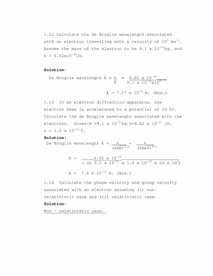
1.12 Calculate the de Broglie wavelength associated

with an electron travelling with a velocity of 105 ms-1.

Assume the mass of the electron to be 9.1 x 10-31kg. and

h = 6.62x10-34Js.

Solution:

De Broglie wavelength λ = h = P 9.1 x 10-31x105

6.62 x 10-34____

λ = 7.27 x 10-9 m. (Ans.) 1.13 In an electron diffraction apparatus, the

electron beam is accelerated to a potential of 25 kV.

Calculate the de Broglie wavelength associated with the

electrons. Given:m =9.1 x 10-31kg,h=6.62 x 10-34 JS.

e = 1.6 x 10-19 C.

Solution: De Broglie wavelength λ = __h___ = ___h___ (2mE)1/2 (2meV)1/2

λ = _____6.62 x 10-34

( 2x 9.1 x 10-31 x 1.6 x 10-19 x 25 x 103) _______________________

λ = 7.6 x 10-12 m. (Ans.) 1.14 Calculate the phase velocity and group velocity

associated with an electron assuming (i) non-

relativistic case and (ii) relativistic case.

Solution:

Non – relativistic case.

Phase velocity vp = ω = (E/ħ) = E = (p2/2m) = p = K (p/ħ) p p 2m 2

v

Phase velocity is half the particle velocity. Group velocity vg = dω = dE = d(p2/2m) = p_ dk dp dp m

= v

Group velocity is equal to the particle velocity.

Relativistic case:

Phase velocity vp = E p

where E = (p2c2 + mo2c4)1/2

∴ vp = c [ 1+ mo2c2

p2 ]1/2

Phase velocity is greater than c. This indicates that

we cannot talk of phase velocity of a particle since it

is represented by a group of waves or a wave packet.

Group velocity vg = dE = _d_ dp dp

[p2c2+moc4]1/2

= pc2 {p2c2 + mo2c4]-1/2 = E

pc2

= mvc2 mc2

= v assuming E = mc2

Group velocity is equal to the particle velocity.

1.15 An electron is trapped in a one dimensional

potential well of infinite depth and a width of

1x10-10 m. What is the probability of finding the

electron in the region from x = 0.09 x 10-10 m to

x = 0.11 x 10-10 m in the ground state.

Solution:

The probability of finding an electron in the region

between x1 and x2 is given by

Method I:

x2 x2 Pn = ∫ψ*ψ dx = (2/L) ∫ sin2(2nπx/L)dx x1 x1 x2

= [x/L – (1/2nπ).sin(2nπx/L)] x1 For ground state, n = 1. x2

P1 = [x/L – (1/2π).sin(2πx/L)] x1 = [0.11-(1/2x3.14)sin(2x180x0.11/1.0)]

-[0.09-(1/2x3.14)sin(2x180x0.09/1.0)]

= (0.11 – 0.10150) – (0.09 – 0.08532)

= 0.00382 (Ans).

The probability of finding an electron in the region of

width ∆x around x is given by

Method II:

Pn = |ψn|2. ∆x = (2/L) sin2(2nπx/L). ∆x

Here, we take n = 1, x = 1x10-10m and ∆x = 0.02x10-10m.

P1 = (2/1x10-10) sin2(1x180x0.1). 0.02x10-10

= 0.00382 (Ans).

Note: The second method is only approximate and gives

result close to the one obtained by method I only when

∆x is very small.

1.16 An electron is trapped in a one dimensional

potential well of width 1x10-10 m and infinite height.

Find the amount of energy required to excite the

electron to its first excited state. What is the

probability of finding the electron in its first

excited state between x =0.4x10-10 m and x =0.6x10-10 m?

Solution:

Energy of the electron in the nth excited state is given by En = 8mL2

n2h2

Energy required to take the electron from ground state

(n = 1) to the first excited state (n = 2) is given by

E = E2 – E1 = h2__(22-12) = 8mL2 8mL2

3h2__

= 8 x 9.1 x 10-31 x (10-10)2

3 x (6.62 x 10-34)2_______

= 1.81 x 10-17 J = 112.87 eV. (Ans.)

The probability of finding the electron in the first

excited state between x = 0.4 A° and x = 0.6 A° is

given by

x2 x2 ∫ψ*ψ dx = (2/L) ∫ sin2(2πx/L)dx x1 x1 x2

= [x/L – (1/4π).sin(4πx/L)] x1

= (0.6 – 0.076) –(0.4 + 0.076)

= 0.048 (Ans)

1.17 The velocity of an electron is measured to be

3x106 ms-1 in a particular direction. If the velocity

is measured with a precision of 1%, what is the

accuracy with which its position can be measured

simultaneously?

Solution:

Momentum of the electron (in non – relativistic

calculation) is

Px = mvx = 9.1 x 10-31 x 3 x 106 = 2.73x10-24kg.m.s-1

Uncertainty in momentum = ∆px = 1% of px

= 2.73x10-26 kg.ms-1

∴ Uncertainty in position, ∆x ≈ ∆px

ħ

= 3.86 x 10-9 m (Ans.)

1.18 In an experimental study of nuclear decay, the

emitted energy spectrum shows a peak with a spread of

energy equal to 120 MeV. Compute the life time of the

decaying nuclei.

Solution: Life time of the decaying nuclei = ∆t ≈ _ ∆E

ħ_

∆t =____6.62 x 10-34

120 x 106 x 1.6 x 10-19 x 2 x 3.14 ___________________

= 5.5 x 10-24 s. (Ans.) 1.19 Calculate the de Broglie wavelength associated

with the following:

(a) A car of mass 1000 kg moving with a velocity

of 50 ms-1

(b) A tennis ball of mass 50 gms moving at a speed

of 75 ms-1.

(c) An air molecule of average mass 2x10-26kg

moving with a velociity of 300 ms-1.

(d) An electron with an energy of 1 MeV.

Solution:

The deBroglie wavelength can be calculated as

λ = h/p

(a) λ = 6.62 x 10-34/1000x50 = 1.324 x 10-38m.This value

is too low to be observable.

(b) λ = 6.62 x 10-34/50 x 10-3x75 = 1.765 x 10-34m.

(c) λ = 6.62 x 10-34/2 x 10-26 x 300 = 1.103 x 10-10m.

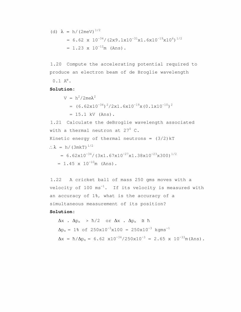
(d) λ = h/(2meV)1/2

= 6.62 x 10-34/(2x9.1x10-31x1.6x10-19x106)1/2

= 1.23 x 10-12m (Ans).

1.20 Compute the accelerating potential required to

produce an electron beam of de Broglie wavelength

0.1 A°.

Solution:

V = h2/2meλ2

= (6.62x10-34)2/2x1.6x10-19x(0.1x10-10)2

= 15.1 kV (Ans).

1.21 Calculate the deBroglie wavelength associated

with a thermal neutron at 270 C.

Kinetic energy of thermal neutrons = (3/2)kT

∴λ = h/(3mkT)1/2

= 6.62x10-34/(3x1.67x10-27x1.38x10-23x300)1/2

= 1.45 x 10-10m (Ans).

1.22 A cricket ball of mass 250 gms moves with a

velocity of 100 ms-1. If its velocity is measured with

an accuracy of 1%, what is the accuracy of a

simultaneous measurement of its position?

Solution:

∆x . ∆px > ħ/2 or ∆x . ∆px ≅ ħ

∆px = 1% of 250x10-3x100 = 250x10-3 kgms-1

∆x = ħ/∆px = 6.62 x10-34/250x10-3 = 2.65 x 10-33m(Ans).

1.23 In a gamma decay process, the life time of

decaying nuclei is found to be 2 ns. Compute the

uncertainty in the energy of gamma rays emitted.

Solution:

∆E . ∆t ≥ ħ/2 or ∆E . ∆t ≅ ħ

∆E = ħ/∆t = 6.62 x 10-34/2 x 3.14 x 2 x 10-9

= 5.27 x 10-26 J (Ans).

EXERCISE

1.1 Explain photoelectric effect. Give the assumptions

needed, and the laws of photoelectric emission.

Calculate the velocity of the photoelectrons emitted

from a metal surface whose work function is 1.5 eV and

the wavelength of the incident light being 4x10-7m.

(March 99)

1.2 Describe the ultraviolet catastrophe. Explain how

the Planck’s law of radiation overcomes it. (March 99)

1.3 Explain Wien’s law and Rayleigh-Jean’s law.

Mention their drawbacks. (August 99)

1.4 Explain Einstein’s theory of photo-electric

effect. (August 99)

1.5 What is Planck’s radiation law? Show how Wien’s

law and Rayleigh-Jean’s law can be derived from it.

(August 99)

1.6 The work function of tungsten is 5.4 eV. When

light of wavelength 170 nm is incident on the surface,

electrons with energy 1.7 eV are ejected. Estimate the

Planck’s constant. (August 99)

1.7 What is the nature of black body radiation?

Explain its significance. (March 2000)

1.8 In Compton scattering, calculate the maximum

kinetic energy of the scattered electron for a given

photon energy. A metal surface has a photoelectric cut

off wavelength of 325.6 nm. What is the stopping

potential for an incident light of wavelength of 259.8

nm? (March 2000)

1.9 State Compton effect and explain the experimental

observations of Compton shift. (August 2000)

1.10 The stopping potential of 5.2 V was observed for

light of frequency 3 x 1015 Hz. What would be the

frequency of light when the stopping potential is

doubled? (August 2000)

1.11 State and explain Planck’s law of radiation. Show

that it reduces to Wien’s law and Rayleigh-Jean’s law

under certain conditions. (August 2000)

1.12 The photoelectric threshold for a certain metal is

5000 AU. Determine the maximum energy of the

photoelectrons emitted when a radiation of wavelength

3000 AU is incident on its surface. (March 01)

1.13 Explain Planck’s radiation law. Discuss Einstein’s

theory of photoelectric effect. (March 01)

1.14 Explain Wien’s Displacement law. Mention its

drawbacks. (August 01)

1.15 Explain Compton effect and give its physical

significance. (August 01)

1.16 What is ultraviolet catastrophe? Show how it can

be overcome with the help of Planck’s radiation law.

(August 01)

1.17 What is photoelectric effect? Mention the features

of photoelectric emission. (March 02)

1.18 What is Compton scattering? With necessary

equations, explain Compton scattering effect.(March 02)

1.19 Calculate the change in wavelength in Compton

scattering at an angle of 600 to the incident

direction. (March02)

1.20 Calculate the wavelength associated with an

electron carrying an energy 2000 eV. (March 99)

1.21 Set up one dimensional Schrodinger’s wave equation

for a free particle. (March 99)

1.22 Explain group velocity and phase velocity. Derive

a relation between the two. (August 99)

1.23 Explain Heisenberg’s uncertainty principle. Give

its physical significance. (August 99)

1.24 What is de Broglie’s concept of matter waves? An

electron has a wavelength of 1.66 x 10-10m. Find the

kinetic energy, phase velocity and group velocityof the

de Broglie wave. (August 99)

1.25 Explain Heisenberg’s uncertainty principle.

Give its physical significance. The position of an

electron can be measured with an accuracy of 1.5 x 10-

10m. Find the uncertainty in its position after 1 sec.

(August 2001)

1.26 What are Eigen functions and Eigen values?

Find them for a particle in one dimensional potential

well of infinite height. (August

2001)

1.27 Obtain the time independent Schrodinger’s wave

equation for a particle in one dimensional potential

well of infinite height and discuss the solution.

(August 2000)

1.28 Write a note on group velocity and phase

velocity. (March 2001)

1.29 Explain group velocity and phase velocity.

Derive relation between the two.

(August 2001)

1.30 What is a wave function? Give its physical

significance. What is normalization of a wave function?

(August 2001)

1.31 What is de Broglie concept of matter waves?

Derive an expression for de Broglie wavelength.

(August 2001)

1.32 Set up time independent Schrodinger’s wave

equation and explain Eigen functions and Eigen values.

(August 99)

1.33 What is Heisenberg’s uncertainty principle?

Discuss its consequences. (March 2000)

1.34 Explain the behaviour of a particle in a one-

dimensional infinite potential well in terms of de

Broglie waves. (March 2000)

1.35 What is the physical interpretation of wave

function, nature of Eigen values and Eigen functions.

(March 2000)

1.36 Discuss phase velocity and group velocity. (August

2000)

1.37 Explain only the conclusions drawn in

photoelectric effect and Davisson-Germer experiment

leading to deBroglie hypothesis. (Feb 2005)

1.38 Show that a free electron cannot exist in a

nucleus of an atom. (Feb 2005)

1.39 What are matter waves? Show that the electron

accelerated by a potential difference V volt is =

1.226/ √V nm for non-relativistic case.(July 2005)

1.40 Explain phase velocity and group velocity. Derive

the expression for deBroglie wavelength using the

concept of group velocity.(July 2005)

1.41 Explain only the conclusions drawn in

photoelectric effect and Davisson-Germer experiment

leading to deBroglie hypothesis. (Feb 2005)

1.42 Show that a free electron cannot exist in a

nucleus of an atom. (Feb 2005)