Chapter 1 - · PDF fileChapter 1 Disk Storage, Basic File Structures, and Hashing. Adapted...
61
1 Chapter 1 Disk Storage, Basic File Structures, and Hashing. Adapted from the slides of “Fundamentals of Database Systems” (Elmasri et al., 2006)
Transcript of Chapter 1 - · PDF fileChapter 1 Disk Storage, Basic File Structures, and Hashing. Adapted...

1
Chapter 1
Disk Storage, Basic File Structures,
and Hashing.
Adapted from the slides of “Fundamentals of Database Systems”
(Elmasri et al., 2006)

2
Chapter Outline
Disk Storage Devices
Files of Records
Operations on Files
Unordered Files
Ordered Files
Hashed Files
Dynamic and Extendible Hashing Techniques
RAID Technology

3
Disk Storage Devices
Preferred secondary storage device for high
storage capacity and low cost.
Data stored as magnetized areas on
magnetic disk surfaces.
A disk pack contains several magnetic disks
connected to a rotating spindle.
Disks are divided into concentric circular
tracks on each disk surface .
Track capacities vary typically from 10 to 150
Kbytes.

Disk Storage Devices (cont.)
4

Disk Storage Devices (cont.)
5
Sector
Track
Spindle

6
Disk Storage Devices (cont.)
A track is divided into smaller blocks or
sectors.
because a track usually contains a large amount
of information .
A track is divided into blocks.
The block size B is fixed for each system.
Typical block sizes range from B=512 bytes to
B=8192 bytes.
Whole blocks are transferred between disk and
main memory for processing.

7
Disk Storage Devices (cont.) A read-write head moves to the track that contains the
block to be transferred. Disk rotation moves the block under the read-write head for
reading or writing.
A physical disk block (hardware) address consists of: a cylinder number (imaginary collection of tracks of same
radius from all recorded surfaces)
the track number or surface number (within the cylinder)
and block number (within track).
Reading or writing a disk block is time consuming because of the seek time s and rotational delay (latency) rd.
Double buffering can be used to speed up the transfer of contiguous disk blocks.
8

Double Buffering
9

10
Records
Fixed and variable length records.
Records contain fields which have values of a
particular type.
E.g., amount, date, time, age.
Fields themselves may be fixed length or
variable length.
Variable length fields can be mixed into one
record:
Separator characters or length fields are needed
so that the record can be “parsed”.

Records (cont.)
11
12
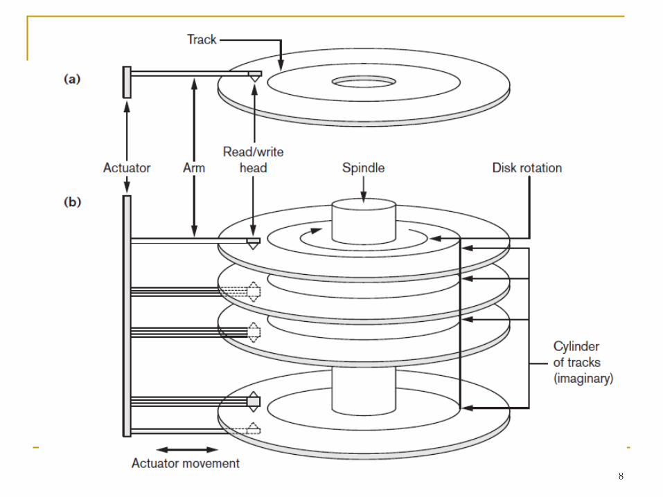
Blocking
Blocking: refers to storing a number of records in one block on the disk.
Blocking factor (bfr): refers to the number of records per block.
There may be empty space in a block if an integral number of records do not fit in one block.
Spanned Records: refer to records that exceed the size of one or more blocks and hence span a number of blocks.

Blocking (cont.)
13

14
Files of Records
A file is a sequence of records, where each record is
a collection of data values (or data items).
A file descriptor (or file header) includes information
that describes the file, such as the field names and
their data types, and the addresses of the file blocks
on disk.
Records are stored on disk blocks.
The blocking factor bfr for a file is the (average)
number of file records stored in a disk block.
A file can have fixed-length records or variable-
length records.

15
Files of Records (cont.)
File records can be unspanned or spanned:
Unspanned: no record can span two blocks
Spanned: a record can be stored in more than one block
The physical disk blocks that are allocated to hold the records of a file can be contiguous, linked, or indexed.
In a file of fixed-length records, all records have the same format. Usually, unspanned blocking is used with such files.
Files of variable-length records require additional information to be stored in each record, such as separator characters and field types.
Usually spanned blocking is used with such files.

16
Operation on Files
Typical file operations include:
OPEN: Reads the file for access, and associates a pointer that will refer to a current file record at each point in time.
FIND: Searches for the first file record that satisfies a certain condition, and makes it the current file record.
FINDNEXT: Searches for the next file record (from the current record) that satisfies a certain condition, and makes it the current file record.
READ: Reads the current file record into a program variable.
INSERT: Inserts a new record into the file, and makes it the current file record.

17
Operation on Files (cont.)
DELETE: Removes the current file record from the file, usually by marking the record to indicate that it is no longer valid.
MODIFY: Changes the values of some fields of the current file record.
CLOSE: Terminates access to the file.
REORGANIZE: Reorganizes the file records. For example, the records marked deleted are physically removed from the file or a new organization of the file records is created.
READ_ORDERED: Read the file blocks in order of a specific field of the file.

18
Unordered Files
Also called a heap or a pile file.
New records are inserted at the end of the file.
A linear search through the file records is
necessary to search for a record.
This requires reading and searching half the file
blocks on the average, and is hence quite expensive.
Record insertion is quite efficient.
Reading the records in order of a particular field
requires sorting the file records.

19
Ordered Files
Also called a sequential file.
File records are kept sorted by the values of an orderingfield.
Insertion is expensive: records must be inserted in the correct order. It is common to keep a separate unordered overflow (or
transaction) file for new records to improve insertion efficiency; this is periodically merged with the main ordered file.
A binary search can be used to search for a record on its ordering field value. This requires reading and searching log2 of the file blocks on the
average, an improvement over linear search.
Reading the records in order of the ordering field is quite efficient.

20
Ordered Files
(cont.)

21
Average Access Times
The following table shows the average access time
to access a specific record for a given type of file:

22
Hashed Files
Hashing for disk files is called External Hashing.
The file blocks are divided into M equal-sized buckets, numbered bucket0, bucket1, ..., bucketM-1. Typically, a bucket corresponds to one (or a fixed number of) disk
block.
One of the file fields is designated to be the hash key of the file.
The record with hash key value K is stored in bucket i, where i=h(K), and h is the hashing function.
Search is very efficient on the hash key.
Collisions occur when a new record hashes to a bucket that is already full. An overflow file is kept for storing such records.
Overflow records that hash to each bucket can be linked together.

Hashed Files (cont.)
23

24
Hashed Files (cont.)
There are numerous methods for collision resolution:
Open addressing: Proceeding from the occupied position specified by the hash address, the program checks the subsequent positions in order until an unused (empty) position is found. h(K) = K mod 7
Insert 8
Insert 15
Insert 13
0 1 2 3 4 5 6
1 3 11 6
1 8 3 11 6
1 8 3 11 15 6
13 1 8 3 11 15 6

25
Hashed Files (cont.)
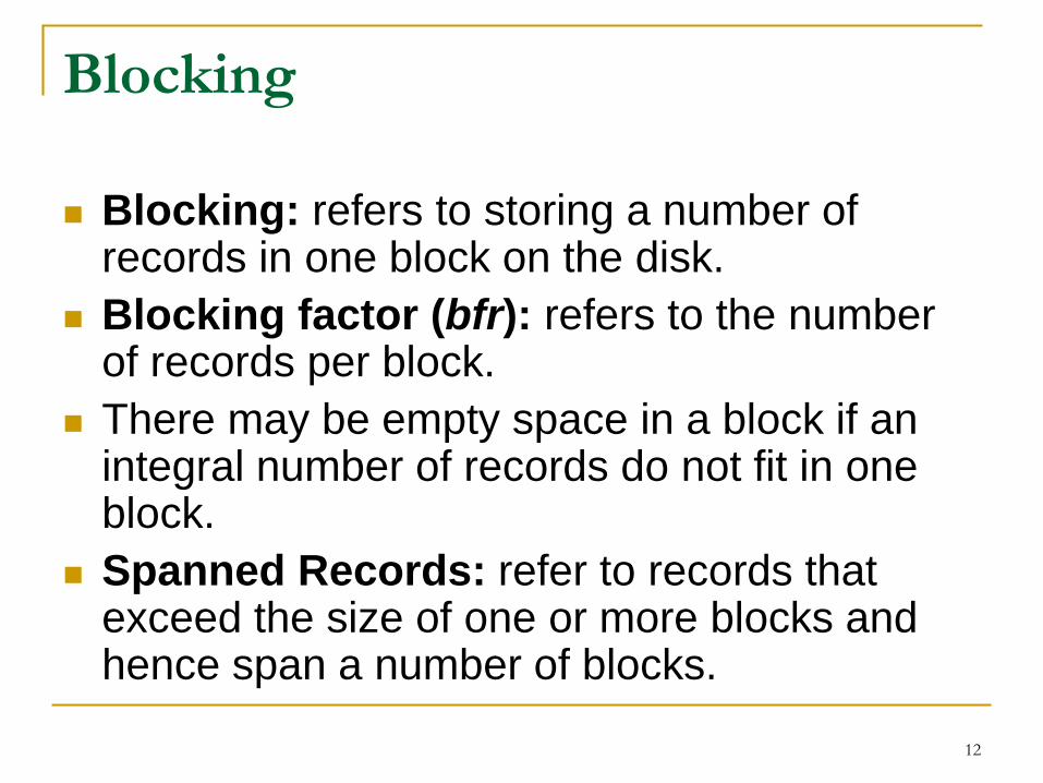
There are numerous methods for collision resolution, including the following: Chaining:
Various overflow locations are kept: extending the array with a number of overflow positions.
A pointer field is added to each record location.
A collision is resolved by placing the new record in an unused overflow location and setting the pointer of the occupied hash address location to the address of that overflow location.
Multiple hashing:
The program applies a second hash function if the first results in a collision.
If another collision results, the program uses open addressing or applies a third hash function and then uses open addressing if necessary.
Hashed Files (cont.) - Overflow handling
26

27
Hashed Files (cont.)
To reduce overflow records, a hash file is typically
kept 70-80% full.
The hash function h should distribute the records
uniformly among the buckets;
Otherwise, search time will be increased because many
overflow records will exist.
Main disadvantages of static external hashing:
Fixed number of buckets M is a problem if the number of
records in the file grows or shrinks.
Ordered access on the hash key is quite inefficient
(requires sorting the records).

28
Dynamic And Extendible Hashed Files
Dynamic and Extendible Hashing Techniques
Hashing techniques are adapted to allow the dynamic
growth and shrinking of the number of file records.
These techniques include the following: dynamic
hashing, extendible hashing, and linear hashing.
Both dynamic and extendible hashing use the
binary representation of the hash value h(K) in
order to access a directory.
In dynamic hashing the directory is a binary tree.
In extendible hashing the directory is an array of size
2d where d is called the global depth.
29
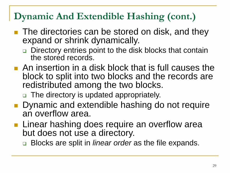
Dynamic And Extendible Hashing (cont.)
The directories can be stored on disk, and they expand or shrink dynamically. Directory entries point to the disk blocks that contain
the stored records.
An insertion in a disk block that is full causes the block to split into two blocks and the records are redistributed among the two blocks. The directory is updated appropriately.
Dynamic and extendible hashing do not require an overflow area.
Linear hashing does require an overflow area but does not use a directory. Blocks are split in linear order as the file expands.

Extendible
Hashing
30
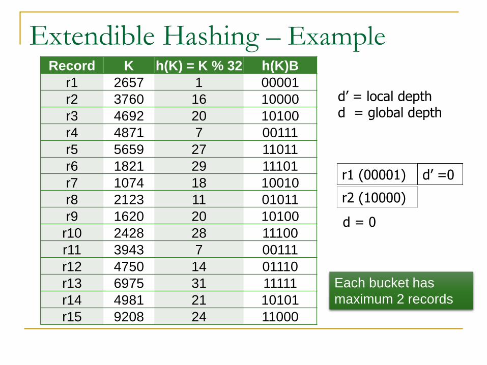
Extendible Hashing – ExampleRecord K h(K) = K % 32 h(K)B
r1 2657 1 00001
r2 3760 16 10000
r3 4692 20 10100
r4 4871 7 00111
r5 5659 27 11011
r6 1821 29 11101
r7 1074 18 10010
r8 2123 11 01011
r9 1620 20 10100
r10 2428 28 11100
r11 3943 7 00111
r12 4750 14 01110
r13 6975 31 11111
r14 4981 21 10101
r15 9208 24 11000
r1 (00001)
r2 (10000)
d’ =0
d = 0
d’ = local depthd = global depth
Each bucket has
maximum 2 records

Insert r3 (10100) => overflow=> splitting
Extendible Hashing – Example(cont.)
r1 (00001)
r2 (10000)
d’ =0
d = 0
Directory
0
1
d = 1
r1 (00001) d’ =1
r2 (10000)
r3 (10100)
d’ =1
Insert r4 (00111)

Insert r5 (11011) => overflow=> splitting
Extendible Hashing – Example(cont.)
01
d = 1
r1 (00001)
r4 (00111)
d’ =1
r2 (10000)
r3 (10100)
d’ =1

Extendible Hashing – Example(cont.)
00
01
10
11
d = 2
r1 (00001)
r4 (00111)
d’ =1
r2 (10000)
r3 (10100)
d’ =2
r5 (11011) d’ =2
Insert r6 (11101)
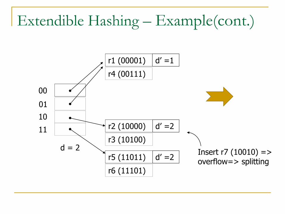
Extendible Hashing – Example(cont.)
Insert r7 (10010) => overflow=> splitting
00
01
10
11
d = 2
r1 (00001)
r4 (00111)
d’ =1
r2 (10000)
r3 (10100)
d’ =2
r5 (11011)
r6 (11101)
d’ =2

Extendible Hashing – Example(cont.)
Insert r8 (01011) => overflow=> splitting
010
011
100
101
000
001
110
111
d = 3
r1 (00001)
r4 (00111)
d’ =1
r3 (10100) d’ =3
r5 (11011)
r6 (11101)
d’ =2
r2 (10000)
r7 (10010)
d’ =3

Extendible Hashing – Example(cont.)
Insert r9 (10100)
010
011
100
101
000
001
110
111
d = 3
r8 (01011) d’ =2
r3 (10100) d’ =3
r5 (11011)
r6 (11101)
d’ =2
r2 (10000)
r7 (10010)
d’ =3
r1 (00001)
r4 (00111)
d’ =2

Extendible Hashing – Example(cont.)
010
011
100
101
000
001
110
111
d = 3
r8 (01011) d’ =2
r3 (10100)
r9 (10100)
d’ =3
r5 (11011)
r6 (11101)
d’ =2
r2 (10000)
r7 (10010)
d’ =3
r1 (00001)
r4 (00111)
d’ =2
Insert r10 (11100) => overflow=> splitting

Extendible Hashing – Example(cont.)
Insert r11 (00111) => overflow=> splitting
010
011
100
101
000
001
110
111
d = 3
r8 (01011) d’ =2
r3 (10100)
r9 (10100)
d’ =3
r5 (11011) d’ =3
r2 (10000)
r7 (10010)
d’ =3
r1 (00001)
r4 (00111)
d’ =2
r6 (11101)
r10 (11100)
d’ =3

Extendible Hashing – Example(cont.)
Insert r12 (01110)010
011
100
101
000
001
110
111
d = 3
r8 (01011) d’ =2
r3 (10100)
r9 (10100)
d’ =3
r5 (11011) d’ =3
r2 (10000)
r7 (10010)
d’ =3
r1 (00001) d’ =3
r6 (11101)
r10 (11100)
d’ =3
r4 (00111)
r11 (00111)
d’ =3

Extendible Hashing – Example(cont.)
Insert r13 (11111) => overflow=> splitting
010
011
100
101
000
001
110
111
d = 3
r8 (01011)
r12 (01110)
d’ =2
r3 (10100)
r9 (10100)
d’ =3
r5 (11011) d’ =3
r2 (10000)
r7 (10010)
d’ =3
r1 (00001) d’ =3
r6 (11101)
r10 (11100)
d’ =3
r4 (00111)
r11 (00111)
d’ =3

Extendible Hashing – Example(cont.)
Insert r14 (10101) => overflow=> splitting
00100011
00000001
01100111
01000101
10101011
10001001
11101111
11001101
d = 4
r8 (01011)
r12 (01110)
d’ =2
r3 (10100)
r9 (10100)
d’ =3
r5 (11011) d’ =3
r2 (10000)
r7 (10010)
d’ =3
r1 (00001) d’ =3
r1 (11111) d’ =4
r4 (00111)
r11 (00111)
d’ =3
r6 (11101)
r10 (11100)
d’ =4
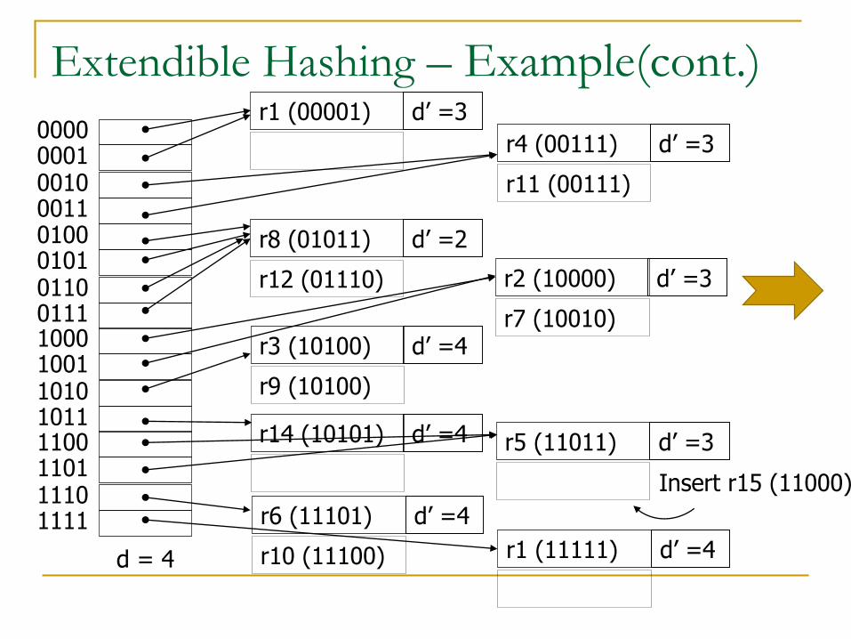
Extendible Hashing – Example(cont.)
Insert r15 (11000)
00100011
00000001
01100111
01000101
10101011
10001001
11101111
11001101
d = 4
r8 (01011)
r12 (01110)
d’ =2
r3 (10100)
r9 (10100)
d’ =4
r5 (11011) d’ =3
r2 (10000)
r7 (10010)
d’ =3
r1 (00001) d’ =3
r1 (11111) d’ =4
r4 (00111)
r11 (00111)
d’ =3
r6 (11101)
r10 (11100)
d’ =4
r14 (10101) d’ =4
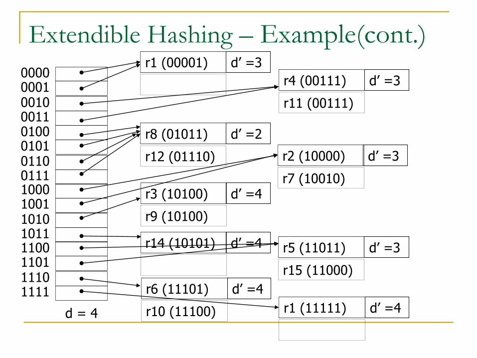
Extendible Hashing – Example(cont.)
00100011
00000001
01100111
01000101
10101011
10001001
11101111
11001101
d = 4
r8 (01011)
r12 (01110)
d’ =2
r3 (10100)
r9 (10100)
d’ =4
r5 (11011)
r15 (11000)
d’ =3
r2 (10000)
r7 (10010)
d’ =3
r1 (00001) d’ =3
r1 (11111) d’ =4
r4 (00111)
r11 (00111)
d’ =3
r6 (11101)
r10 (11100)
d’ =4
r14 (10101) d’ =4

M=4, h0(K) = K mod M, each bucket has 3
records.
Initialization:
Linear Hashing – Example
0 1 2 3
4 : 8 : 5 : 9 : 13 6 : : 7 : 11 :
Split pointer
Insert 17 (17 mod 4 = 1)
Bucket 1: overflow
Split bucket 0
h1(K) = K mod 2*M

Linear Hashing – Example(cont.)
0 1 2 3 4
8 : : 5 : 9 : 13 6 : : 7 : 11 : 4 : :
Split pointer
17 : :
4: bucket (4 mod 2*4 =) 4
8: bucket (8 mod 2*4 = ) 0
17: overflow records

Linear Hashing – Example(cont.)
0 1 2 3 4
8 : : 5 : 9 : 13 6 : : 7 : 11 : 4 : :
Split pointer
17 : :
insert 15 (15 mod 4 = 3)

Linear Hashing – Example(cont.)
0 1 2 3 4
8 : : 5 : 9 : 13 6 : : 7 : 11 : 15 4 : :
Split pointer
17 : :
insert 3 (3 mod 4 = 3)
Bucket 3: overflow
Split bucket 1.
=> Overflow records: Redistributed

Linear Hashing – Example(cont.)
0 1 2 3 4 5
8 : : 9 : 17 : 6 : : 7 : 11 : 15 4 : : 5 : 13 :
Split pointer
3 : :
5: bucket (5 mod 2*4 =) 5
9: bucket (9 mod 2*4 = ) 1
13: bucket (13 mod 2*4 = ) 5
17: bucket (17 mod 2*4 = ) 1

Linear Hashing – Example(cont.)
0 1 2 3 4 5
8 : : 9 : 17 : 6 : : 7 : 11 : 15 4 : : 5 : 13 :
Split pointer
3 : :
Insert 23 (23 mod 4 = 3)
Bucket 3: overflow.
Split bucket 2.

Linear Hashing – Example(cont.)
0 1 2 3 4 5 6
8 : : 9 : 17 : : : 7 : 11 : 15 4 : : 5 : 13 : 6 : :
Split pointer
3 : 23 :
insert 31(31 mod 4 = 3)
Bucket 3: overflow
Split bucket 3
=> Overflow records: Redistributed

Linear Hashing – Example(cont.)
0 1 2 3 4 5 6 7
8 : : 9 : 17 : : : 11 : 15 : 3 4 : : 5 : 13 : 6 : : 7 : 23 : 31
Split pointer
7: bucket (7 mod 2*4 =) 7
11: bucket (11 mod 2*4 = ) 3
15: bucket (15 mod 2*4 = ) 3
3: bucket (3 mod 2*4 = ) 3
23: bucket (23 mod 2*4 = ) 7
31: bucket (31 mod 2*4 = ) = 7
h1(K) = K mod 8

53
Parallelizing Disk Access using RAID
Technology.
Secondary storage technology must take steps to
keep up in performance and reliability with
processor technology.
A major advance in secondary storage technology is
represented by the development of RAID, which
originally stood for Redundant Arrays of
Inexpensive Disks.
The main goal of RAID is to even out the widely
different rates of performance improvement of disks
against those in memory and microprocessors.

54
RAID Technology (cont.)
A natural solution is a large array of small independent disks acting as a single higher-performance logical disk. A concept called data striping is used, which utilizes parallelism to improve disk performance.
Data striping distributes data transparently over multiple disks to make them appear as a single large, fast disk.

55
RAID Technology (cont.)
Different raid organizations were defined based on different combinations of the two factors of granularity of data interleaving (striping) and pattern used to compute redundant information. Raid level 0 has no redundant data and hence has the best write
performance.
Raid level 1 uses mirrored disks.
Raid level 2 uses memory-style redundancy by using Hamming codes, which contain parity bits for distinct overlapping subsets of components. Level 2 includes both error detection and correction.

56
RAID Technology (cont.) Raid level 3 uses a single parity disk relying on the disk controller to
figure out which disk has failed.
Raid levels 4 and 5 use block-level data striping, with level 5 distributing data and parity information across all disks.

57
RAID Technology (cont.) Raid level 6 applies the so-called P + Q redundancy scheme using
Reed-Soloman codes to protect against up to two disk failures by using just two redundant disks.

58
Use of RAID Technology (cont.) Different raid organizations are being used under
different situations: Raid level 1 (mirrored disks) is the easiest for rebuild of a disk
from other disks
It is used for critical applications like logs.
Raid level 2 uses memory-style redundancy by using Hamming codes, which contain parity bits for distinct overlapping subsets of components. Level 2 includes both error detection and correction.
Raid level 3 (single parity disks relying on the disk controller to figure out which disk has failed) and level 5 (block-level data striping) are preferred for large volume storage, with level 3 giving higher transfer rates.
Most popular uses of the RAID technology currently are: Level 0 (with striping), Level 1 (with mirroring) and Level 5 with an extra drive for parity.
Design decisions for RAID include – level of RAID, number of disks, choice of parity schemes, and grouping of disks for block-level striping.

59
Storage Area Networks
The demand for higher storage has risen considerably in recent times.
Organizations have a need to move from a static fixed data center oriented operation to a more flexible and dynamic infrastructure for information processing.
Thus they are moving to a concept of Storage Area Networks (SANs).
In a SAN, online storage peripherals are configured as nodes on a high-speed network and can be attached and detached from servers in a very flexible manner.
This allows storage systems to be placed at longer distances from the servers and provide different performance and connectivity options.

60
Storage Area Networks (cont.)
Advantages of SANs are:
Flexible many-to-many connectivity among servers and
storage devices using fiber channel hubs and switches.
Up to 10km separation between a server and a storage
system using appropriate fiber optic cables.
Better isolation capabilities allowing nondisruptive addition
of new peripherals and servers.
SANs face the problem of:
combining storage options from multiple vendors
dealing with evolving standards of storage management
software and hardware.

Review questions1) What is the difference between a file organization and an
access method?
2) What is the difference between static and dynamic files?
3) What are the typical record-at-a-time operations for accessing
a file? Which of these depend on the current record of a file?
4) Discuss the advantages and disadvantages of (a) unordered
file, (b) ordered file, and (c) static hash file with buckets and
chaining. Which operations can be performed efficiently on
each of these organizations, and which operations are
expensive?
5) Discuss the techniques for allowing a hash file to expand and
shrink dynamically. What are the advantages and
disadvantages of each?
61