Chapter 08.01 Primer for Ordinary Differential Equations
26
Chapter 08.01 Primer for Ordinary Differential Equations After reading this chapter, you should be able to: 1. define an ordinary differential equation, 2. differentiate between an ordinary and partial differential equation, and 3. solve linear ordinary differential equations with fixed constants by using classical solution and Laplace transform techniques. Introduction An equation that consists of derivatives is called a differential equation. Differential equations have applications in all areas of science and engineering. Mathematical formulation of most of the physical and engineering problems leads to differential equations. So, it is important for engineers and scientists to know how to set up differential equations and solve them. Differential equations are of two types (A) ordinary differential equations (ODE) (B) partial differential equations (PDE) An ordinary differential equation is that in which all the derivatives are with respect to a single independent variable. Examples of ordinary differential equations include 0 2 2 2 = + + y dx dy dx y d , 4 ) 0 ( , 2 ) 0 ( = = y dx dy , , sin 5 3 2 2 3 3 x y dx dy dx y d dx y d = + + + , 12 ) 0 ( 2 2 = dx y d 2 ) 0 ( = dx dy , 4 ) 0 ( = y Ordinary differential equations are classified in terms of order and degree. Order of an ordinary differential equation is the same as the highest derivative and the degree of an ordinary differential equation is the power of highest derivative. Thus the differential equation, x e xy dx dy x dx y d x dx y d x = + + + 2 2 2 3 3 3 08.01.1
Transcript of Chapter 08.01 Primer for Ordinary Differential Equations
Chapter 08.01 Primer for Ordinary Differential Equations After reading this chapter, you should be able to:
1. define an ordinary differential equation, 2. differentiate between an ordinary and partial differential equation, and 3. solve linear ordinary differential equations with fixed constants by using classical
solution and Laplace transform techniques. Introduction An equation that consists of derivatives is called a differential equation. Differential equations have applications in all areas of science and engineering. Mathematical formulation of most of the physical and engineering problems leads to differential equations. So, it is important for engineers and scientists to know how to set up differential equations and solve them. Differential equations are of two types (A) ordinary differential equations (ODE) (B) partial differential equations (PDE)
An ordinary differential equation is that in which all the derivatives are with respect to a single independent variable. Examples of ordinary differential equations include
022
2
=++ ydxdy
dxyd , 4)0( ,2)0( == y
dxdy ,
,sin53 2
2
3
3
xydxdy
dxyd
dxyd
=+++ ,12)0(2
2
=dx
yd 2)0( =dxdy , 4)0( =y
Ordinary differential equations are classified in terms of order and degree. Order of an ordinary differential equation is the same as the highest derivative and the degree of an ordinary differential equation is the power of highest derivative. Thus the differential equation,
xexydxdyx
dxydx
dxydx =+++ 2
22
3
33
08.01.1

08.01.2 Chapter 08.01
is of order 3 and degree 1, whereas the differential equation
xdxdyx
dxdy sin1 2
2
=+⎟⎠⎞
⎜⎝⎛ +
is of order 1 and degree 2. An engineer’s approach to differential equations is different from a mathematician. While, the latter is interested in the mathematical solution, an engineer should be able to interpret the result physically. So, an engineer’s approach can be divided into three phases:
a) formulation of a differential equation from a given physical situation, b) solving the differential equation and evaluating the constants, using given conditions,
and c) interpreting the results physically for implementation.
Formulation of differential equations As discussed above, the formulation of a differential equation is based on a given physical situation. This can be illustrated by a spring-mass-damper system.
Above is the schematic diagram of a spring-mass-damper system. A block is suspended freely using a spring. As most physical systems involve some kind of damping - viscous damping, dry damping, magnetic damping, etc., a damper or dashpot is attached to account for viscous damping.
Kb
x
Figure 1 Spring-mass damper system.
M
Let the mass of the block be M , the spring constant be K , and the damper coefficient be b . If we measure displacement from the static equilibrium position we need not consider gravitational force as it is balanced by tension in the spring at equilibrium. Below is the free body diagram of the block at static and dynamic equilibrium. So, the equation of motion is given by (1) DS FFMa +=where is the restoring force due to spring. SF
Primer for Ordinary Differential Equation 08.01.3
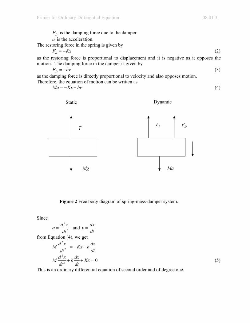
is the damping force due to the damper. DF is the acceleration. aThe restoring force in the spring is given by (2) KxFS −=as the restoring force is proportional to displacement and it is negative as it opposes the motion. The damping force in the damper is given by (3) bvFD −=as the damping force is directly proportional to velocity and also opposes motion. Therefore, the equation of motion can be written as (4) bvKxMa −−=
Since
SF
Ma
Dynamic Static
Mg
T DF
Figure 2 Free body diagram of spring-mass-damper system.
2
2
dtxda = and
dtdxv =
from Equation (4), we get
dtdxbKx
dtxdM −−=2
2
02
2
=++ Kxdtdxb
dtxdM (5)
This is an ordinary differential equation of second order and of degree one.

08.01.4 Chapter 08.01
Solution to linear ordinary differential equations In this section we discuss two techniques used to solve ordinary differential equations (A) Classical technique (B) Laplace transform technique
Classical Technique The general form of a linear ordinary differential equation with constant coefficients is given by
)(......... 122
2
31
1
xFykdxdyk
dxydk
dxydk
dxyd
n
n
nn
n
=+++++ −
−
(6)
The general solution contains two parts (7) PH yyy +=where is the homogeneous part of the solution and Hy is the particular part of the solution. PyThe homogeneous part of the solution is that part of the solution that gives zero when substituted in the left hand side of the equation. So, is solution of the equation
Hy
Hy
0......... 122
2
31
1
=+++++ −
−
ykdxdyk
dxydk
dxydk
dxyd
n
n
nn
n
(8)
The above equation can be symbolically written as (9) 0................. 12
1 =++++ − ykDykyDkyD nn
n
(10) 0).................( 121 =++++ − ykDkDkD n
nn
where,
n
nn
dxdD = (11)
.
.
.
1
11
−
−− = n
nn
dxdD
operating on y is the same as , ),( 1rD − )( 2rD − )( nrD −operating one after the other in any order, where )(....,),........(),( 21 nrDrDrD −−− are factors of 0 (12) ............... 12
1 =++++ − kDkDkD nn
n
To illustrate 0)23( 2 =+− yDDis same as
Primer for Ordinary Differential Equation 08.01.5
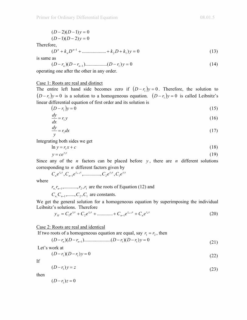
0)1)(2( =−− yDD 0)2)(1( =−− yDDTherefore, (13) 0)....................( 12
1 =++++ − ykDkDkD nn
n
is same as 0).........().........)(( 11 =−−− − yrDrDrD nn (14) operating one after the other in any order. Case 1: Roots are real and distinct The entire left hand side becomes zero if ( ) 01 =− yrD . Therefore, the solution to
is a solution to a homogeneous equation. ( ) 01 =− yrD ( ) 01 =− yrD is called Leibnitz’s linear differential equation of first order and its solution is (15) ( ) 01 =− yrD
yrdxdy
1= (16)
dxry
dy1= (17)
Integrating both sides we get (18) cxry += 1ln (19) xrcey 1=Since any of the factors can be placed before , there are different solutions corresponding to different factors given by
n y nn
xrxrxrn
xrn eCeCeCeC nn 121
121 ,.....,,........., −−
where are the roots of Equation (12) and 121, ,..,,......... rrrr nn −
are constants. 121, ,,......, CCCC nn −
We get the general solution for a homogeneous equation by superimposing the individual Leibnitz’s solutions. Therefore (20) xr
nxr
nxrxr
Hnn eCeCeCeCy ++++= −
−121
121 ............. Case 2: Roots are real and identical If two roots of a homogeneous equation are equal, say 21 rr = , then
0))(...(..........).........)(( 111 =−−−− − yrDrDrDrD nn (21) Let’s work at (22) 0))(( 11 =−− yrDrDIf (23) zyrD =− )( 1
then 0)( 1 =− zrD

08.01.6 Chapter 08.01
(24) xreCz 12=
Now substituting the solution from Equation (24) in Equation (23) xreCyrD 1
21 )( =−
xreCyrdxdy
121 =−
2111 Cyer
dxdye xrxr =− −−
2)( 1
Cdx
yed xr
=−
(25) dxCyed xr2)( 1 =−
Integrating both sides of Equation (25), we get 12
1 CxCye xr +=−
(26) xreCxCy 1)( 12 +=Therefore the final homogeneous solution is given by (27) ( ) xr
nxrxr
HneCeCexCCy ++++= ...31
321
Similarly, if m roots are equal the solution is given by ( ) xr
nxr
mxrm
mHnmm eCeCexCxCxCCy +++++++= +
+− .......... 1
112
321 (28) Case 3: Roots are complex If one pair of roots is complex, say βα ir +=1 and βα ir −=2 , where 1−=i then (29) ( ) ( ) xr
nxrxixi
HneCeCeCeCy ++++= −+ ......3
321βαβα
Since , and (30a) xixe xi βββ sincos += (30b) xixe xi βββ sincos −=−
then ( ) ( ) xr
nxrxx
HneCeCxixeCxixeCy +++−++= .........sincossincos 3
321 ββββ αα ( ) ( ) xr
nxrxx neCeCxeCCixeCC +++−++= .........sincos 3
32121 ββ αα
(31) ( ) xrn
xrx neCeCxBxAe ++++= ........sincos 33ββα
where and 21 CCA += (32) )( 21 CCiB −=Now, let us look at how the particular part of the solution is found. Consider the general form of the ordinary differential equation ( ) XykDkDkD n
nn
nn =++++ −
−−
12
11 .......... (33)
The particular part of the solution is that part of solution that gives Py X when substituted for y in the above equation, that is,

Primer for Ordinary Differential Equation 08.01.7
( ) XykDkDkD Pn
nn
nn =++++ −
−−
12
11 ...... (34)
Sample Case 1 When , the particular part of the solution is of the form . We can find axeX = axAe A by substituting in the left hand side of the differential equation and equating coefficients.
axAey =
Example 1 Solve
xeydxdy −=+ 23 , 5)0( =y
Solution
The homogeneous solution for the above equation is given by ( ) 023 =+ yDThe characteristic equation for the above equation is given by 023 =+rThe solution to the equation is 666667.0−=r x
H Cey 666667.0−=The particular part of the solution is of the form xAe−
( ) xxx
eAedxAed −−
−
=+ 23
xxx eAeAe −−− =+− 23 xx eAe −− =− 1−=AHence the particular part of the solution is x
P ey −−=The complete solution is given by PH yyy += xx eCe −− −= 666667.0 The constant can be obtained by using the initial condition C 5)0( =y ( ) 50 00666667.0 =−= −×− eCey 51 =−C 6=CThe complete solution is xx eey −− −= 666667.06 Example 2 Solve
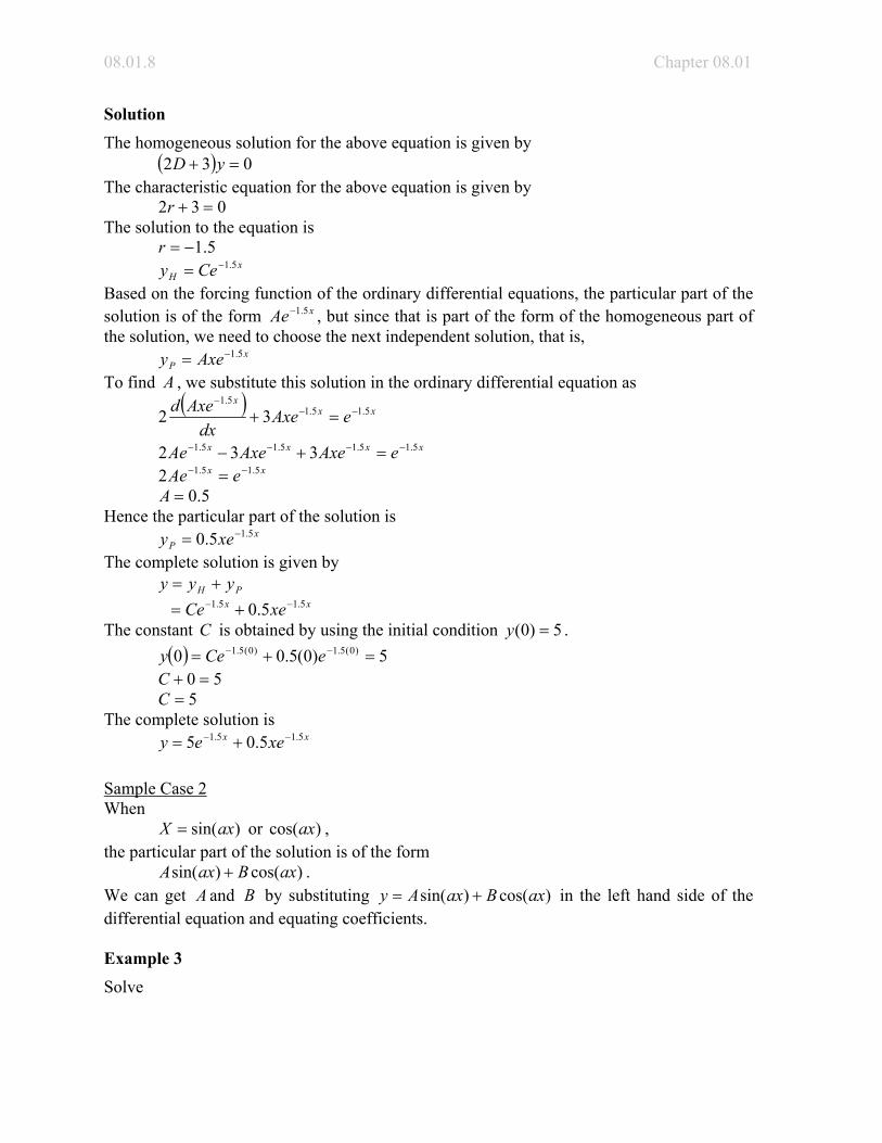
xeydxdy 5.132 −=+ , 5)0( =y
08.01.8 Chapter 08.01
Solution The homogeneous solution for the above equation is given by ( ) 032 =+ yDThe characteristic equation for the above equation is given by 032 =+rThe solution to the equation is 5.1−=r x
H Cey 5.1−=Based on the forcing function of the ordinary differential equations, the particular part of the solution is of the form , but since that is part of the form of the homogeneous part of the solution, we need to choose the next independent solution, that is,
xAe 5.1−
xP Axey 5.1−=
To find A , we substitute this solution in the ordinary differential equation as
( ) xxx
eAxedx
Axed 5.15.15.1
32 −−−
=+
xxxx eAxeAxeAe 5.15.15.15.1 332 −−−− =+− xx eAe 5.15.12 −− = 5.0=AHence the particular part of the solution is x
P xey 5.15.0 −=The complete solution is given by PH yyy += xx xeCe 5.15.1 5.0 −− +=The constant is obtained by using the initial condition C 5)0( =y . ( ) 5)0(5.00 )0(5.1)0(5.1 =+= −− eCey 50 =+C 5=CThe complete solution is xx xeey 5.15.1 5.05 −− += Sample Case 2 When or , )sin(axX = )cos(ax
)the particular part of the solution is of the form . cos()sin( axBaxA +We can get and A B by substituting )cos()sin( axBaxAy += in the left hand side of the differential equation and equating coefficients. Example 3 Solve

Primer for Ordinary Differential Equation 08.01.9
xydxdy
dxyd sin125.332 2
2
=++ , 3)0( ,5)0( === xdxdyy
Solution
The homogeneous equation is given by 0)125.332( 2 =++ yDDThe characteristic equation is 0125.332 2 =++ rrThe roots of the characteristic equation are
22
125.32433 2
×××−±−
=r
4
2593 −±−=
4
163 −±−=
4
43 i±−=
i±−= 75.0 Therefore the homogeneous part of the solution is given by )sincos( 21
75.0 xKxKey xH += −
The particular part of the solution is of the form
xBxAyP cossin +=
( ) ( ) xxBxAxBxAdxdxBxA
dxd sin)cossin(125.3cossin3cossin2 2
2
=+++++
( ) xxBxAxBxAxBxAdxd sin)cossin(125.3)sincos(3sincos2 =++−+−
xxBxAxBxAxBxA sin)cossin(125.3)sincos(3)cossin(2 =++−+−− xxABxBA sincos)3125.1(sin)3125.1( =++− Equating coefficients of and xsin xcos on both sides, we get 13125.1 =− BA 03125.1 =+ ABSolving the above two simultaneous linear equations we get 109589.0=A 292237.0−=BHence xxyP cos292237.0sin109589.0 −=The complete solution is given by )cos292237.0sin109589.0()sincos( 21
75.0 xxxKxKey x −++= −
To find and we use the initial conditions 1K 2K
3)0( ,5)0( === xdxdyy
From we get 5)0( =y

08.01.10 Chapter 08.01
))0cos(292237.0)0sin(109589.0())0sin()0cos((5 21)0(75.0 −++= − KKe
292237.05 1 −= K 292237.51 =K
xx
xKxKexKxKedxdy xx
sin292237.0cos109589.0
)cossin()sincos(75.0 2175.0
2175.0
++
+−++−= −−
From
,3)0( ==xdxdy
we get
)0sin(292237.0)0cos(109589.0
))0cos()0sin(( ))0sin()0cos((75.03 21)0(75.0
21)0(75.0
+++−++−= −− KKeKKe
109589.075.03 21 ++−= KK 109589.0)292237.5(75.03 2 ++−= K 859588.62 =KThe complete solution is xxxxey x cos292237.0sin109589.0)sin859588.6cos292237.5(75.0 −++= −
Example 4 Solve
)cos(125.362 2
2
xydxdy
dxyd
=++ , 3)0( ,5)0( === xdxdyy
Solution The homogeneous part of the equations is given by 0)125.362( 2 =++ yDDThe characteristic equation is given by 0125.362 2 =++ rr
)2(2
)125.3)(2(466 2 −±−=r
4
25366 −±−=
4
116 ±−=
829156.05.1 ±−= 329156.2,670844.0 −−=Therefore, the homogeneous solution is given by Hy xx
H eKeKy 329156.22
670845.01
−− +=The particular part of the solution is of the form xBxAyP cossin +=
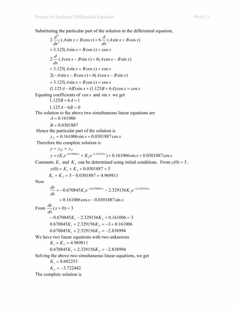
Primer for Ordinary Differential Equation 08.01.11
Substituting the particular part of the solution in the differential equation,
xxBxA
xBxAdxdxBxA
dxd
cos)cossin(125.3
)cossin(6)cossin(2 2
2
=++
+++
xxBxA
xBxAxBxAdxd
cos)cossin(125.3
)sincos(6)sincos(2
=++
−+−
xxBxA
xBxAxBxAcos)cossin(125.3
)sincos(6)cossin(2=++
−+−−
xxABxBA coscos)6125.1(sin)6125.1( =++− Equating coefficients of xcos and we get xsin
06125.116125.1
=−=+
BAAB
The solution to the above two simultaneous linear equations are
0301887.0161006.0
==
BA
Hence the particular part of the solution is xxyP cos0301887.0sin161006.0 += Therefore the complete solution is PH yyy += xxeKeKy xx cos0301887.0sin161006.0)( 329156.2
2670845.0
1 +++= −−
Constants and can be determined using initial conditions. From , 1K 2K 5)0( =y 50301887.0)0( 21 =++= KKy 969811.40301887.0521 =−=+ KK Now
xx
eKeKdxdy xx
sin0301887.0cos161006.0
329156.2670845.0 )329156.2(2
)670845.0(1
−+
−−= −−
From 3)0( ==xdxdy
3161006.0329156.2670845.0 21 =+−− KK 161006.03329156.2670845.0 21 +−=+ KK 838994.2329156.2670845.0 21 −=+ KK We have two linear equations with two unknowns 969811.421 =+ KK 838994.2329156.2670845.0 21 −=+ KK Solving the above two simultaneous linear equations, we get 692253.81 =K 722442.32 −=KThe complete solution is

08.01.12 Chapter 08.01
.cos0301887.0sin161006.0
)722442.3692253.8( 329156.2670845.0
xxeey xx
++−= −−
Sample Case 3 When or , bxeX ax sin= bxeax costhe particular part of the solution is of the form
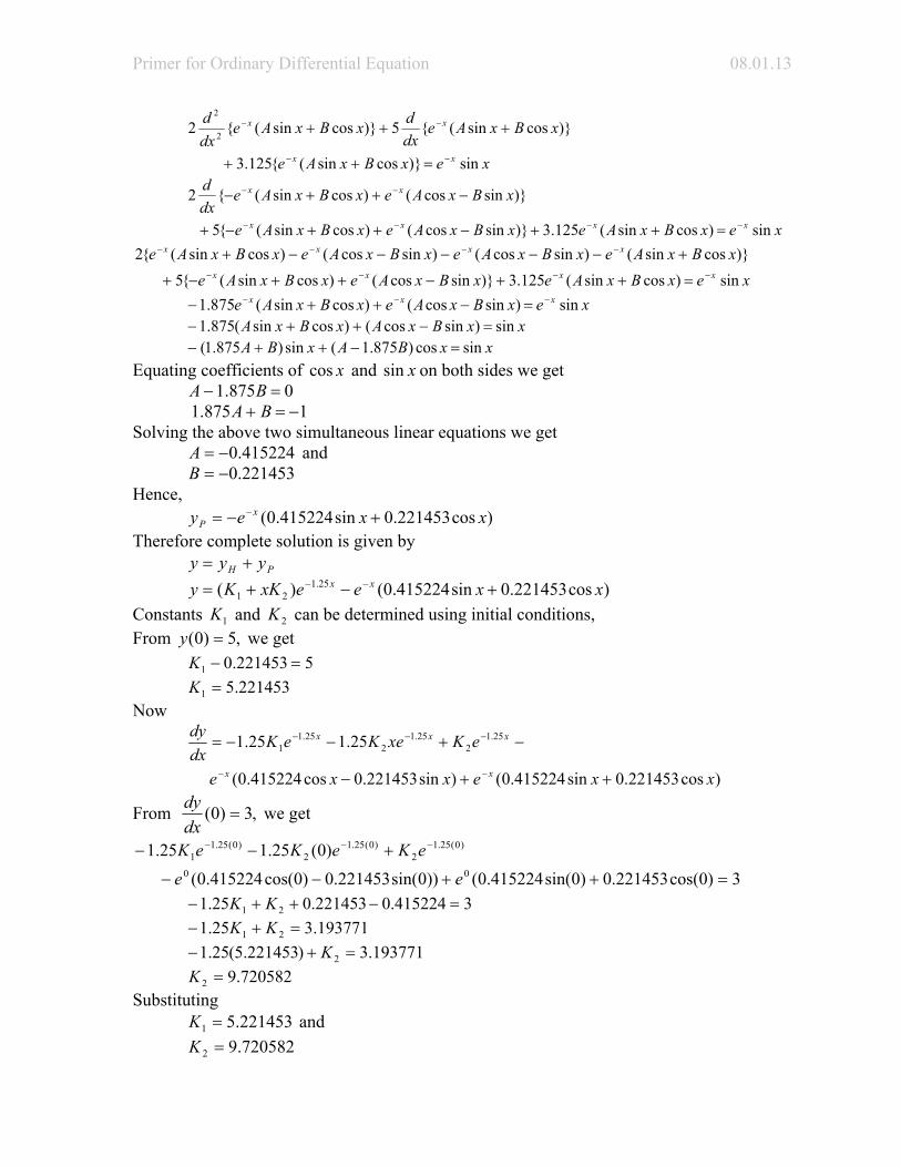
)cossin( bxBbxAeax + , we can get and A B by substituting )cossin( bxBbxAey ax +=in the left hand side of differential equation and equating coefficients. Example 5 Solve
xeydxdy
dxyd x sin125.352 2
2−=++ , 3)0( ,5)0( === x
dxdyy
Solution The homogeneous equation is given by 0)125.352( 2 =++ yDD The characteristic equation is given by 0125.352 2 =++ rr
)2(2
)125.3)(2(455 2 −±−=r
4
25255 −±−=
4
05 ±−=
25.1,25.1 −−=Since roots are repeated, the homogeneous solution is given by Hy x
H exKKy )25.1(21 )( −+=
The particular part of the solution is of the form )cossin( xBxAey x
P += −
Substituting the particular part of the solution in the ordinary differential equation
Primer for Ordinary Differential Equation 08.01.13
xexBxAe
xBxAedxdxBxAe
dxd
xx
xx
sin)}cossin({125.3
)}cossin({5)}cossin({2 2
2
−−
−−
=++
+++
xexBxAexBxAexBxAe
xBxAexBxAedxd
xxxx
xx
sin)cossin(125.3)}sincos()cossin({5
)}sincos()cossin({2
−−−−
−−
=++−++−+
−++−
xexBxAexBxAexBxAexBxAexBxAexBxAexBxAe
xxxx
xxxx
sin)cossin(125.3)}sincos()cossin({5 )}cossin()sincos()sincos()cossin({2
−−−−
−−−−
=++−++−+
+−−−−−+
xexBxAexBxAe xxx sin)sincos()cossin(875.1 −−− =−++− xxBxAxBxA sin)sincos()cossin(875.1 =−++− xxBAxBA sincos)875.1(sin)875.1( =−++− Equating coefficients of xcos and on both sides we get xsin 0875.1 =− BA 1875.1 −=+ BASolving the above two simultaneous linear equations we get and 415224.0−=A 221453.0−=BHence, )
)
cos221453.0sin415224.0( xxey xP +−= −
Therefore complete solution is given by PH yyy += cos221453.0sin415224.0()( 25.1
21 xxeexKKy xx +−+= −−
Constants and can be determined using initial conditions, 1K 2KFrom we get ,5)0( =y 5221453.01 =−K 221453.51 =KNow
)cos221453.0sin415224.0()sin221453.0cos415224.0(
25.125.1 25.12
25.12
25.11
xxexxe
eKxeKeKdxdy
xx
xxx
++−
−+−−=
−−
−−−
From ,3)0( =dxdy we get
3)0cos(221453.0)0sin(415224.0())0sin(221453.0)0cos(415224.0(
)0(25.125.100
)0(25.12
)0(25.12
)0(25.11
=++−−
+−− −−−
ee
eKeKeK
3415224.0221453.025.1 21 =−++− KK 193771.325.1 21 =+− KK 193771.3)221453.5(25.1 2 =+− K 720582.92 =KSubstituting and 221453.51 =K 720582.92 =K

08.01.14 Chapter 08.01
in the solution, we get )cos221453.0sin415224.0()720582.9221453.5( 25.1 xxeexy xx +−+= −−
The forms of the particular part of the solution for different right hand sides of ordinary differential equations are given below
X ( )xyP 2
210 xaxaa ++ 2210 xbxbb ++
axe axAe )sin(bx )cos()sin( bxBbxA +
)sin(bxeax ( ))cos()sin( bxBbxAeax +
)cos(bx )cos()sin( bxBbxA +
)cos(bxeax ( ))cos()sin( bxBbxAeax + Laplace Transforms
If is defined at all positive values of )(xfy = x , the Laplace transform denoted by is given by
)(sY
(35) dxxfexfLsY sx )()}({)(0∫∞
−==
where is a parameter, which can be a real or complex number. We can get back by taking the inverse Laplace transform of .
s )(xf)(sY
(36) )()}({1 xfsYL =−
Laplace transforms are very useful in solving differential equations. They give the solution directly without the necessity of evaluating arbitrary constants separately. The following are Laplace transforms of some elementary functions
sL 1)1( =
1
!)( += nn
snxL , where ....3,2,1,0=n
as
eL ax
−=
1)(
22)(sinas
aaxL+
=
22)(cosas
saxL+
=
22)(sinhas
aaxL−
=

Primer for Ordinary Differential Equation 08.01.15
22)(coshas
saxL−
= (37)
The following are the inverse Laplace transforms of some common functions
111 =⎟⎠⎞
⎜⎝⎛−
sL
axeas
L =⎟⎠⎞
⎜⎝⎛
−− 11
( )!11 1
1
−=⎟
⎠⎞
⎜⎝⎛ −
−
nx
sL
n
n , where ......3,2,1=n
( ) ( )!1
1 11
−=⎟⎟
⎠
⎞⎜⎜⎝
⎛
−
−−
nxe
asL
nax
n
axaas
L sin1122
1 =⎟⎠⎞
⎜⎝⎛
+−
axas
sL cos221 =⎟
⎠⎞
⎜⎝⎛
+−
axaas
L sinh1122
1 =⎟⎠⎞
⎜⎝⎛
−−
atas
sL cosh221 =⎟
⎠⎞
⎜⎝⎛
−−
( )
bxebbas
L ax sin1122
1 =⎟⎟⎠
⎞⎜⎜⎝
⎛
+−−
( )
bxebas
asL ax cos22
1 =⎟⎟⎠
⎞⎜⎜⎝
⎛
+−−−
( )
axxaas
sL sin21
222
1 =⎟⎟⎠
⎞⎜⎜⎝
⎛
+− (38)
Properties of Laplace transforms
Linear property If are constants and and are functions of cba , , ),( ),( xgxf )(xh x then ))(())(())(()]()()([ xhcLxgbLxfaLxchxbgxafL ++=++ (39) Shifting property If (40) )()}({ sYxfL =then (41) )()}({ asYxfeL at −=Using shifting property we get

08.01.16 Chapter 08.01
( )( ) 1
!+−
= nnax
asnxeL , 0≥n
( )( ) 22sin
basbbxeL ax
+−=
( )( ) 22cos
basasbxeL ax
+−−
=
( )( ) 22sinh
basbbxeL ax
−−=
( )( ) 22cosh
basasbxeL ax
−−−
= (42)
Scaling property If (43) )()}({ sYxfL =then
⎟⎠⎞
⎜⎝⎛=
asY
aaxfL 1)}({ (44)
Laplace transforms of derivatives
If the first n derivatives of are continuous then )(xf
(45) ∫∞
−=0
)()}({ dxxfexfL nsxn
Using integration by parts we get
∫
∫∞
−
∞∞
−−−−−
−−−−−
−−+
⎥⎥⎦
⎤
⎢⎢⎣
⎡
−−++−+
−−=
0
001132
21
)()()1(
)()()1(......)()()()()(
)(
dxxfes
xfesxfesxfesxfe
dxxfe
sxnn
sxnnnsx
nsxnsxnsx
∫∞
−−−−− +−−−−−=0
13221 )()0(.............)0()0()0( dxxfesfsfssff sxnnnnn
(46) )0(........)0()0()0()( 13221 fsfssffsYs nnnnn −−−− −−−−−= Laplace transform technique to solve ordinary differential equations
The following are steps to solve ordinary differential equations using the Laplace transform method (A) Take the Laplace transform of both sides of ordinary differential equations. (B) Express )(sY as a function of s . (C) Take the inverse Laplace transform on both sides to get the solution.
Let us solve Examples 1 through 4 using the Laplace transform method.
Primer for Ordinary Differential Equation 08.01.17
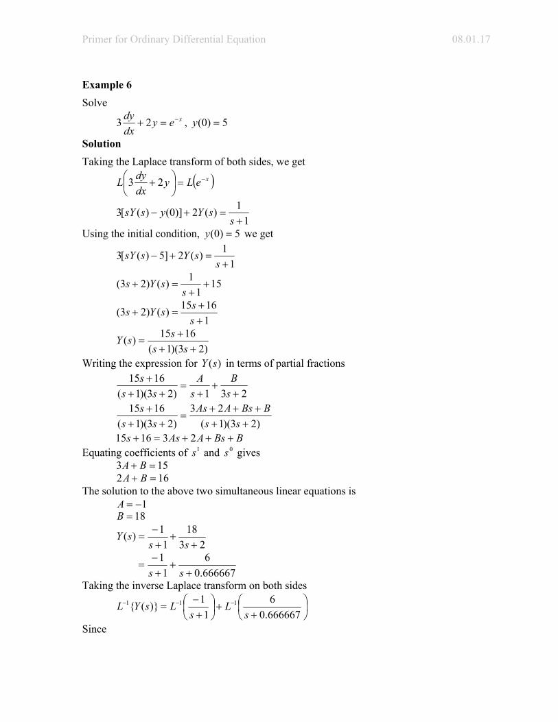
Example 6 Solve
xeydxdy −=+ 23 , 5)0( =y
Solution Taking the Laplace transform of both sides, we get
( )xeLydxdyL −=⎟
⎠⎞
⎜⎝⎛ + 23
1
1)(2)]0()([3+
=+−s
sYyssY
Using the initial condition, 5)0( =y we get
1
1)(2]5)([3+
=+−s
sYssY
151
1)()23( ++
=+s
sYs
11615)()23(
++
=+sssYs
)23)(1(
1615)(++
+=
ssssY
Writing the expression for in terms of partial fractions )(sY
231)23)(1(
1615+
++
=++
+sB
sA
sss
)23)(1(
23)23)(1(
1615++
+++=
+++
ssBBsAAs
sss
BBsAAss +++=+ 231615 Equating coefficients of and gives 1s 0s 153 =+ BA 162 =+ BAThe solution to the above two simultaneous linear equations is 1−=A 18=B
23
181
1)(+
++−
=ss
sY
666667.06
11
++
+−
=ss
Taking the inverse Laplace transform on both sides
⎟⎠⎞
⎜⎝⎛
++⎟
⎠⎞
⎜⎝⎛
+−
= −−−
666667.06
11)}({ 111
sL
sLsYL
Since

08.01.18 Chapter 08.01
ateas
L −− =⎟⎠⎞
⎜⎝⎛
+11
The solution is given by xx eexy 666667.06)( −− +−= Example 7 Solve
xeydxdy 5.132 −=+ , 5)0( =y
Solution Taking the Laplace transform of both sides, we get
( )xeLydxdyL 5.132 −=⎟
⎠⎞
⎜⎝⎛ +
5.1
1)(3)]0()([2+
=+−s
sYyssY
Using the initial condition , we get 5)0( =y
5.1
1)(3]5)([2+
=+−s
sYssY
105.1
1)()32( ++
=+s
sYs
5.11610)()32(
++
=+s
ssYs
)32)(5.1(
1610)(++
+=
ssssY
)5.1)(5.1(2
1610++
+=
sss
2)5.1(21610
++
=s
s
2)5.1(85
++
=s
s
Writing the expression for in terms of partial fractions )(sY
22 )5.1(5.1)5.1(85
++
+=
++
sB
sA
ss
22 )5.1(5.1
)5.1(85
+++
=++
sBAAs
ss
BAAss ++=+ 5.185Equating coefficients of and gives 1s 0s 5=A 85.1 =+ BAThe solution to the above two simultaneous linear equations is

Primer for Ordinary Differential Equation 08.01.19
5=A 5.0=B
2)5.1(5.0
5.15)(
++
+=
sssY
Taking the inverse Laplace transform on both sides
⎟⎟⎠
⎞⎜⎜⎝
⎛+
+⎟⎠⎞
⎜⎝⎛
+= −−−
2111
)5.1(5.0
5.15)}({
sL
sLsYL
Since
axeas
L −− =⎟⎠⎞
⎜⎝⎛
+11 and axxe
asL −− =⎟⎟
⎠
⎞⎜⎜⎝
⎛+ 2
1
)(1
The solution is given by xx xeexy 5.15.1 5.05)( −− += Example 8 Solve
xydxdy
dxyd sin125.332 2
2
=++ , 3)0( ,5)0( === xdxdyy
Solution Taking the Laplace transform of both sides
( )xLydxdy
dxydL sin125.332 2
2
=⎟⎟⎠
⎞⎜⎜⎝
⎛++
and knowing
⎟⎟⎠
⎞⎜⎜⎝
⎛2
2
dxydL ( ) ( ) ( )002 =−−= x
dxdysysYs
⎟⎠⎞
⎜⎝⎛
dxdyL ( ) ( )0yssY −=
1
1)(sin 2 +=
sxL
we get
[ ]1
1)(125.3)0()(3)0()0()(2 22
+=+−+⎥⎦
⎤⎢⎣⎡ =−−
ssYyssYx
dxdysysYs
[ ] [ ]1
1)(125.35)(335)(2 22
+=+−+−−
ssYssYssYs
( )[ ]1
12110)(125.332 2 +=−−++
sssYss
( )[ ] 21101
1)(125.332 2 +++
=++ ss
sYss

08.01.20 Chapter 08.01
[ ])1(
21101022)(125.332 2
232
++++
=++s
ssssYss
( )( )125.332122102110)( 22
23
++++++
=sss
ssssY
Writing the expression for in terms of partial fractions )(sY
( ) ( ) ( )( )125.332122102110
1125.332 22
23
22 ++++++
=++
++++
ssssss
sDCs
ssBAs
( )( )
( )( )125.332122102110
1125.332125.332125.332
22
23
22
22323
++++++
=
++++++++++++
ssssss
sssDDsDsCsCsCsBBsAsAs
( ) ( ) ( ) ( )( )( )
( )( )125.332122102110
125.3321125.33125.3232
22
23
22
23
++++++
=
++++++++++++
ssssss
sssDBsDCAsDCBsCA
Equating terms of , and gives 3s 12 , ss 0s 102 =+ CA 2123 =++ DCB 103125.3 =++ DCA 22125.3 =+ DBThe solution to the above four simultaneous linear equations is 584474.10=A 657534.21=B 292237.0−=C 109589.0=DHence
1
109589.0292237.0125.332657534.21584474.10)( 22 +
+−+
+++
=s
sss
ssY
( ) }1)75.0{(2}1)5625.05.1{(2125.332 222 ++=+++=++ sssss
1
109589.0292237.0}1)75.0{(2
719179.13)75.0(584474.10)( 22 ++−
+++++
=s
ssssY
)1(
109589.0)1(
292237.0}1)75.0{(
859589.6}1)75.0{(
)75.0(292237.5 2222 ++
+−
+++
+++
=ss
sss
s
Taking the inverse Laplace transform of both sides
⎟⎠⎞
⎜⎝⎛
++⎟
⎠⎞
⎜⎝⎛
+−
⎟⎟⎠
⎞⎜⎜⎝
⎛++
+⎟⎟⎠
⎞⎜⎜⎝
⎛++
+=
−−
−−−
1109589.0
1292237.0
1)75.0{(859589.6
}1)75.0{()75.0(292237.5)}({
21
21
21
211
sL
ssL
sL
ssLsYL

Primer for Ordinary Differential Equation 08.01.21
⎟⎠⎞
⎜⎝⎛
++⎟
⎠⎞
⎜⎝⎛
+−
⎟⎟⎠
⎞⎜⎜⎝
⎛++
+⎟⎟⎠
⎞⎜⎜⎝
⎛++
+=
−−
−−−
11109589.0
1292237.0
1)75.0{(1859589.6
}1)75.0{(75.0292237.5)}({
21
21
21
211
sL
ssL
sL
ssLsYL
Since
( )
bxebas
asL ax cos22
1 −− =⎟⎟⎠
⎞⎜⎜⎝
⎛
+++
( )
bxebas
bL ax sin22
1 −− =⎟⎟⎠
⎞⎜⎜⎝
⎛
++
axas
L sin122
1 =⎟⎠⎞
⎜⎝⎛
+−
axas
sL cos221 =⎟
⎠⎞
⎜⎝⎛
+−
The complete solution is
xx
xexexy xx
sin109589.0cos292237.0 sin8595859.6cos292237.5)( 75.075.0
+−+= −−
( ) xxxxe x sin109589.0cos292237.0sin859589.6cos292237.5 75.0 +−+= −
Example 9 Solve
xydxdy
dxyd cos125.362 2
2
=++ , 3)0( ,5)0( === xdxdyy
Solution Taking the Laplace transform of both sides
( )xLydxdy
dxydL cos125.362 2
2
=⎟⎟⎠
⎞⎜⎜⎝
⎛++
and knowing
⎟⎟⎠
⎞⎜⎜⎝
⎛2
2
dxydL ( ) ( ) ( )002 =−−= x
dxdysysYs
⎟⎠⎞
⎜⎝⎛
dxdyL ( ) ( )0yssY −=
1
)(cos 2 +=
ssxL
we get
[ ]1
)(125.3)0()(6)0()0()(2 22
+=+−+⎥⎦
⎤⎢⎣⎡ =−−
sssYyssYx
dxdysysYs
[ ] [ ]1
)(125.35)(635)(2 22
+=+−+−−
sssYssYssYs

08.01.22 Chapter 08.01
[ ] 3610
1)(125.3)62( 2 ++
+=++ s
sssYss
[ ]1
36111036)(125.362 2
232
++++
=++s
ssssYss
( )( )125.362136113610)( 22
23
++++++
=sss
ssssY
Writing the expression for in terms of partial fractions )(sY
( ) ( ) ( )( )125.362136113610
1125.362 22
23
22 ++++++
=++
++++
ssssss
sDCs
ssBAs
( )( )
( )( )125.362136113610
1125.362125.362125.362
22
23
22
22323
++++++
=
++++++++++++
ssssss
sssDDsDsCsCsCsBBsAsAs
( ) ( ) ( ) ( )( )( )
( )( )125.362136113610
125.3621125.36125.3262
22
23
22
23
++++++
=
++++++++++++
ssssss
sssDBsDCAsDCBsCA
Equating terms of , and gives 3s 12 , ss 0s 102 =+ CA 3626 =++ DCB 116125.3 =++ DCA 36125.3 =+ DBThe solution to the above four simultaneous linear equations is 939622.9=A 496855.35=B 0301886.0=C 161006.0=DThen
1
161006.00301886.0125.362496855.35939622.9)( 22 +
++
+++
=s
sss
ssY
( ) }829156.0)5.1{(2}6875.0)25.23{(2125.362 2222 −+=−++=++ sssss
1
161006.00301886.0}829156.0)5.1{(2
587422.20)5.1(939622.9)( 222 ++
+−+
++=
ss
sssY
1161006.0
10301886.0
}829156.0)5.1{(293711.10
}829156.0)5.1{()5.1(969811.4
22
2222
++
++
−++
−++
=
sss
sss
Taking the inverse Laplace transform on both sides
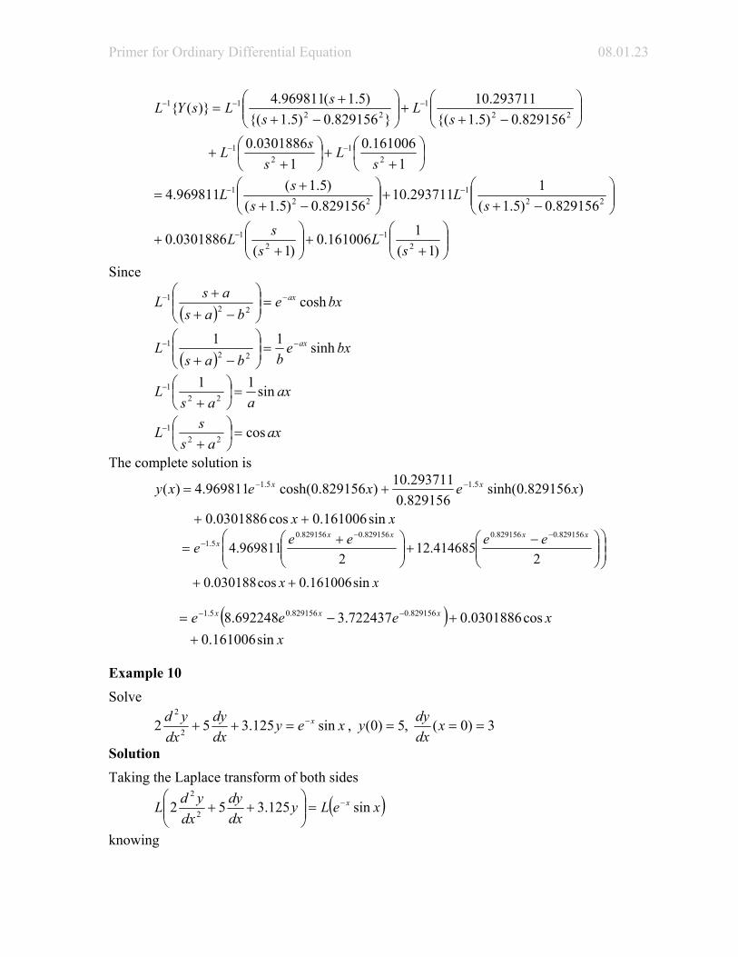
Primer for Ordinary Differential Equation 08.01.23
⎟⎠⎞
⎜⎝⎛
++⎟
⎠⎞
⎜⎝⎛
++
⎟⎟⎠
⎞⎜⎜⎝
⎛−+
+⎟⎟⎠
⎞⎜⎜⎝
⎛−+
+=
−−
−−−
1161006.0
10301886.0
829156.0)5.1{(293711.10
}829156.0)5.1{()5.1(969811.4)}({
21
21
221
2211
sL
ssL
sL
ssLsYL
⎟⎟⎠
⎞⎜⎜⎝
⎛−+
+⎟⎟⎠
⎞⎜⎜⎝
⎛−++
= −−22
122
1
829156.0)5.1(1293711.10
829156.0)5.1()5.1(969811.4
sL
ssL
⎟⎟⎠
⎞⎜⎜⎝
⎛+
+⎟⎟⎠
⎞⎜⎜⎝
⎛+
+ −−
)1(1161006.0
)1(0301886.0 2
12
1
sL
ssL
Since
( )
bxebas
asL ax cosh22
1 −− =⎟⎟⎠
⎞⎜⎜⎝
⎛
−++
( )
bxebbas
L ax sinh1122
1 −− =⎟⎟⎠
⎞⎜⎜⎝
⎛
−+
axaas
L sin1122
1 =⎟⎠⎞
⎜⎝⎛
+−
axas
sL cos221 =⎟
⎠⎞
⎜⎝⎛
+−
The complete solution is
xx
xexexy xx
sin161006.0cos0301886.0
)829156.0sinh(829156.0293711.10)829156.0cosh(969811.4)( 5.15.1
++
+= −−
xx
eeeeexxxx
x
sin161006.0cos030188.0
2414685.12
2969811.4
829156.0829156.0829156.0829156.05.1
++
⎟⎟⎠
⎞⎜⎜⎝
⎛⎟⎟⎠
⎞⎜⎜⎝
⎛ −+⎟⎟
⎠
⎞⎜⎜⎝
⎛ +=
−−−
( )x
xeee xxx
sin161006.0 cos0301886.0722437.3692248.8 829156.0829156.05.1
++−= −−
Example 10
Solve
xeydxdy
dxyd x sin125.352 2
2−=++ , 3)0( ,5)0( === x
dxdyy
Solution Taking the Laplace transform of both sides
( )xeLydxdy
dxydL x sin125.352 2
2−=⎟⎟
⎠
⎞⎜⎜⎝
⎛++
knowing

08.01.24 Chapter 08.01
⎟⎟⎠
⎞⎜⎜⎝
⎛2
2
dxydL ( ) ( ) ( )002 =−−= x
dxdysysYs
⎟⎠⎞
⎜⎝⎛
dxdyL ( ) ( )0yssY −=
1)1(
1)sin( 2 ++=−
sxeL x
we get
[ ]
[ ] [ ]1)1(
1)(125.35)(535)(2
1)1(1)(125.3)0()(5)0()0()(2
22
22
++=+−+−−
++=+−+⎥⎦
⎤⎢⎣⎡ =−−
ssYssYssYs
ssYyssYx
dxdysysYs
( )[ ]
1)1(13110)(125.352 2 ++
=−−++s
ssYss
[ ] 31101)1(
1)(125.3)52( 2 ++++
=++ ss
sYss
[ ]22
51821063)(125.352 2
232
+++++
=++ss
ssssYss
( )( )125.3522263825110)( 22
23
+++++++
=ssssssssY
Writing the expression for in terms of partial fractions )(sY
( )( )125.3522263825110
22125.352 22
23
22 +++++++
=++
++
+++
sssssss
ssDCs
ssBAs
( )( )
( )( )125.3522263825110
22125.3522222125.352125.352
22
23
22
223223
+++++++
=
+++++++++++++++
sssssss
ssssBBsBsAsAsAsDDsDsCsCsCs
( ) ( ) ( ) ( )
( )( )
( )( )125.3522263825110
125.352222125.3225125.32252
22
23
22
23
+++++++
=
+++++++++++++++
sssssss
ssssBDsBADCsBADCsAC
Equating terms of , and gives four simultaneous linear equations 3s 12 , ss 0s 102 =+ AC 51225 =+++ BADC 82225125.3 =+++ BADC 632125.3 =+ BDThe solution to the above four simultaneous linear equations is
Primer for Ordinary Differential Equation 08.01.25
442906.10=A 494809.32=B 221453.0−=C 636678.0−=DThen
22636678.0221453.0
125.352494809.32442906.10)( 22 ++
−−+
+++
=ss
sss
ssY
( ) 222 )25.1(2)}5625.15.2{(2125.352 +=++=++ sssss
1)1(
415225.0)1(221453.0)25.1(2
441176.19)25.1(442906.10)( 22 ++−+−
++
++=
ss
sssY
1)1(
415225.01)1(
)1(221453.0)25.1(
720588.9)25.1(
)25.1(221453.5 2222 ++−
+++
−+
++
+=
sss
sss
Taking the inverse Laplace transform on both sides
⎟⎟⎠
⎞⎜⎜⎝
⎛++
−⎟⎟⎠
⎞⎜⎜⎝
⎛+++
−
⎟⎟⎠
⎞⎜⎜⎝
⎛+
+⎟⎟⎠
⎞⎜⎜⎝
⎛+
=
−−
−−−
1)1(415225.0
1)1()1(221453.0
)25.1(720588.9
)25.1(221453.5)}({
21
21
2111
sL
ssL
sL
sLsYL
⎟⎟⎠
⎞⎜⎜⎝
⎛++
−⎟⎟⎠
⎞⎜⎜⎝
⎛++
+−
⎟⎟⎠
⎞⎜⎜⎝
⎛+
+⎟⎟⎠
⎞⎜⎜⎝
⎛+
=
−−
−−
1)1(1415225.0
1)1()1(221453.0
)25.1(1720588.9
)25.1(1221453.5
21
21
211
sL
ssL
sL
sL
Since
( )
bxebas
asL ax cos22
1 −− =⎟⎟⎠
⎞⎜⎜⎝
⎛
+++
( )
bxebas
bL ax sin22
1 −− =⎟⎟⎠
⎞⎜⎜⎝
⎛
++
axeas
L −− =⎟⎠⎞
⎜⎝⎛
+11
)!1()(
1 11
−=⎟⎟
⎠
⎞⎜⎜⎝
⎛+
−−−
nxe
asL
nax
n
The complete solution is
xe
xexeexyx
xxx
sin415225.0 cos221453.0720588.9221453.5)( 25.125.1
−
−−−
−
−+=
( ) )sin415225.0cos221453.0(720588.9221453.5 25.1 xxexe xx −−++= −
08.01.26 Chapter 08.01
ORDINARY DIFFERENTIAL EQUATIONS Topic A Primer on ordinary differential equations Summary Textbook notes of a primer on solution of ordinary differential equations Major All majors of engineering Authors Autar Kaw, Praveen Chalasani Date April 24, 2009 Web Site http://numericalmethods.eng.usf.edu