FMIA

ISBN 978-3-319-16873-9

Fluid Mechanics and Its ApplicationsFluid Mechanics and Its ApplicationsSeries Editor: A. Thess

F. MoukalledL. ManganiM. Darwish

The Finite Volume Method in Computational Fluid DynamicsAn Advanced Introduction with OpenFOAM® and Matlab®

The Finite Volume Method in Computational Fluid Dynamics

Moukalled · Mangani · Darwish

113

F. Moukalled · L. Mangani · M. Darwish The Finite Volume Method in Computational Fluid Dynamics An Advanced Introduction with OpenFOAM® and Matlab ®

This textbook explores both the theoretical foundation of the Finite Volume Method (FVM) and its applications in Computational Fluid Dynamics (CFD). Readers will discover a thorough explanation of the FVM numerics and algorithms used in the simulation of incompressible and compressible fluid flows, along with a detailed examination of the components needed for the development of a collocated unstructured pressure-based CFD solver. Two particular CFD codes are explored. The first is uFVM, a three-dimensional unstructured pressure-based finite volume academic CFD code, implemented within Matlab®. The second is OpenFOAM®, an open source framework used in the development of a range of CFD programs for the simulation of industrial scale flow problems.

With over 220 figures, numerous examples and more than one hundred exercises on FVM numerics, programming, and applications, this textbook is suitable for use in an introductory course on the FVM, in an advanced course on CFD algorithms, and as a reference for CFD programmers and researchers.

Engineering

9 783319 168739

The Finite Volume Method

Chapter 05

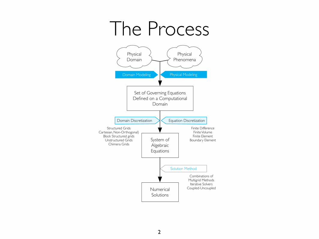
The Process

2

Set of Governing Equations Defined on a Computational

Domain

System of Algebraic Equations

Numerical Solutions

Finite DifferenceFinite VolumeFinite Element

Boundary Element

Combinations ofMultigrid MethodsIterative Solvers

Coupled-Uncoupled

Structured GridsCartesian, Non-Orthogonal)

Block Structured gridsUnstructured Grids

Chimera Grids

Physical Phenomena

Physical Domain

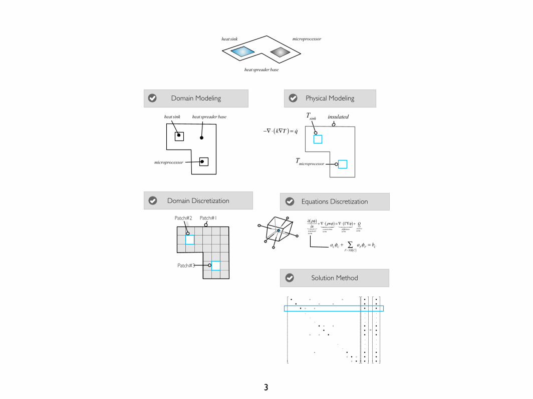
Physical ModelingDomain Modeling

Equation DiscretizationDomain Discretization

Solution Method

3

Patch#3

Patch#2 Patch#1

∂ ρφ( )∂t

transientterm

+∇⋅ ρvφ( )

convectionterm

= ∇⋅ Γ∇φ( )

diffusionterm

+ Qsourceterm

• •

• ...

• •

•

..

• • •

⎡

⎣

⎢⎢⎢⎢⎢⎢⎢⎢⎢⎢⎢⎢⎢⎢⎢⎢⎢⎢⎢

⎤

⎦

⎥⎥⎥⎥⎥⎥⎥⎥⎥⎥⎥⎥⎥⎥⎥⎥⎥⎥⎥

•••...•••...•••

⎡

⎣

⎢⎢⎢⎢⎢⎢⎢⎢⎢⎢⎢⎢⎢⎢⎢⎢⎢⎢⎢

⎤

⎦

⎥⎥⎥⎥⎥⎥⎥⎥⎥⎥⎥⎥⎥⎥⎥⎥⎥⎥⎥

=

•••...•••...•••

⎡

⎣

⎢⎢⎢⎢⎢⎢⎢⎢⎢⎢⎢⎢⎢⎢⎢⎢⎢⎢⎢

⎤

⎦

⎥⎥⎥⎥⎥⎥⎥⎥⎥⎥⎥⎥⎥⎥⎥⎥⎥⎥⎥

Domain Modeling Physical Modeling

Domain Discretization Equations Discretization

Solution Method

aCφC + aFφFF∼NB C( )∑ = bC

Tmicroprocessormicroprocessor

heat spreader baseheat sink Tsink insulated

heat sink

heat spreader base

microprocessor

−∇⋅ k∇T( ) = !q

Balance Form

4

ρvφ( ) ⋅dS∂V!∫ = Γ∇φ( ) ⋅dS

∂V!∫ + QdV

V∫∫

ρvφ( ) ⋅dSf∫

f = faces V( )∑ = Γ∇φ( ) ⋅dS

f∫

f = faces V( )∑ + QdV

V∫∫

∇⋅ ρvφ( )convectionterm!"# $#

= ∇⋅ Γ∇φ( )diffusionterm! "# $# + Qφ

sourceterm!

Consider the steady state conservation equation of a scalar

∇⋅ ρvφ( )dVV∫∫ = ∇⋅ Γ∇φ( )dV

V∫∫ + QdV

V∫∫

∇⋅FdVV∫∫ = F ⋅dS

∂V!∫

Diffusion

Convection

Source/Sink

Transient

S f1

F1

F2

F3

F4F5

F6C

dCN1

f3

f4f5

f6

f2f1

one integration point

FluxTf=

FluxC fφC + FluxFfφF1 + FluxVf

Face Flux Integration

5

�

ρuφ( ) f ⋅S f

�

ρuφ( )1 f( ) ⋅ w1 f( )S f + ρuφ( )2 f( ) ⋅ w2 f( )S f

ρvφ( ) ⋅dSf∫

f = faces V( )∑

J ⋅dSf∫ = J ⋅S( )ip

ip f( )∑ = Jip ⋅wipS f( )

ip f( )∑

two integration points

FluxTf=

FluxC fφC + FluxFfφF1 + FluxVf

S f1

F1

F2

F3

F4F5

F6C

dCN1

f3

f4f5

f6

f2f1

three integration points

FluxTf=

FluxC fφC + FluxFfφF1 + FluxVf

S f1

F1

F2

F3

F4F5

F6C

dCN1

f3

f4f5

f6

f2f1

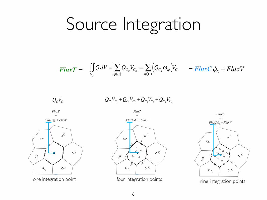
Source Integration

6

QCVC QC1VC1 +QC2

VC2 +QC3VC3 +QC4

VC4

QdVVC∫∫ = QCip

VCipip C( )∑ = QCip

ω ip( )ip C( )∑ VC = FluxCφC + FluxVFluxT =

FluxT=

FluxCφC + FluxV

one integration point

F1

F2

F3

F4F5

F6C

FluxT=

FluxCφC + FluxV

four integration points

f1f2

f3

f4 f5

f6

F1

F2

F3

F4F5

F6C

FluxT=

FluxCφC + FluxV

nine integration points

F1

F2

F3

F4F5

F6C

Flux Linearization

7

J fφ ⋅S f = FluxTf

total fluxfor face f

!"#= FluxC f

flux linearizationcoefficient forC

!"# $#φC + FluxFf

flux linearizationcoefficient for F

!"#φF + FluxVf

non−linearized part!"#

f1f2

f3

f4 f5

f6

F1

F2

F3

F4F5

F6C

J fφ ⋅S f( )

f ∼nb C( )∑ = FluxTf( )

f ∼nb C( )∑

= FluxC f φC +FluxFf φF +FluxVf( )f ∼nb C( )∑

QCφVC = FluxT

= FluxCφC +FluxV

aCφC + aFφF( )F∼NB C( )∑ = bC

aC = FluxC f − FluxCf ∼nb C( )∑

aF = FluxFf

bC = − FluxVf + FluxVf ∼nb C( )∑

b

Sb

eb

C

tn

φb,specified

Boundary Conditions

8

Value Specified (Dirichlet Boundary Condition)

Jbφ ⋅Sb = Jb

φ ,C ⋅Sb= ρvφ( )b ⋅Sb= FluxCbφC +FluxVb= ρbvb ⋅Sb( )φb = !mfφb,specified

FluxCb = 0FluxVb = !mfφb,specified

b

Sb

eb

C

tn qb,specified

Jbφ ⋅Sb = Jb

φ ⋅nbSpecified flux! Sb

= qb, specifiedSb

FluxCb = 0FluxVb = qb, specifiedSb

Flux Specified (Neumann Boundary Condition)

FVM Accuracy

Spatial Variation

10

�

φ(x) = φP + x − xP( ) ⋅ ∇φ( )P + 12 x − xP( )2 : ∇∇φ( )P

+ 13! x − xP( )3 :: ∇∇∇φ( )P + …

+ 1n! x − xP( )n:::

n!(∇∇∇

n" # $ φ)P + …

�

φ(x) = φP + x − xP( ) ⋅ ∇φ( )P + O Δx 2( )

φ x( ) x

xCφC∇φC∇∇φC

Mean Value Theorem

11

φCφC

φC = 1VC

φ dVVC∫

= 1VC

φC + x − xC( ) ⋅ ∇φ( )C +O x − xC2( )⎡

⎣⎤⎦dV

VC∫

= φCVC

dVVC∫ + 1

VCx − xC( ) ⋅ ∇φ( )C dV

VC∫ + 1

VCO x − xC

2( )dVVC∫

= φC +O x − xC2( )

Cell Value flux

Mean Value Theorem

12

C

J fφ ,D ⋅S f = − Γφ∇φ( )

f⋅S f

Diffusion flux! "## $## f

F

J fφ ,C ⋅S f = ρvφ( ) f ⋅S f

Convection flux! "# $#

ρ fv f ⋅S f( )φ f = ρvφ( ) ⋅dSf∫

= ρ fv f φ f + x − x f( ) ⋅ ∇φ( ) f +O x − x f

2( )⎡⎣⎢

⎤⎦⎥⋅dS

f∫

= ρ fv fφ f ⋅ dSf∫ + x − x f( ) ⋅ ∇φ( ) f ρ fv f ⋅dS

f∫ + O x − x f

2( )ρ fv f ⋅dSf∫

= ρ fv f ⋅S f( ) φ f +O x − x f

2( )⎡⎣⎢

⎤⎦⎥

convective flux

Γφ∇φ( ) ⋅dSf∫ = Γφ∇φ( ) f + x − x f( ) ⋅ ∇ Γφ∇φ( )( )

f+O x − x f

2( )⎡⎣⎢

⎤⎦⎥⋅dS

f∫

= Γφ∇φ( ) f ⋅ dSf∫ + x − x f( )dS

f∫⎡

⎣⎢⎢

⎤

⎦⎥⎥: ∇ Γφ∇φ( )( )

f+O x − x f

2( )= Γφ∇φ( ) f ⋅S f +O x − x f

2( )

diffusion flux

Properties of the Discretized Equations

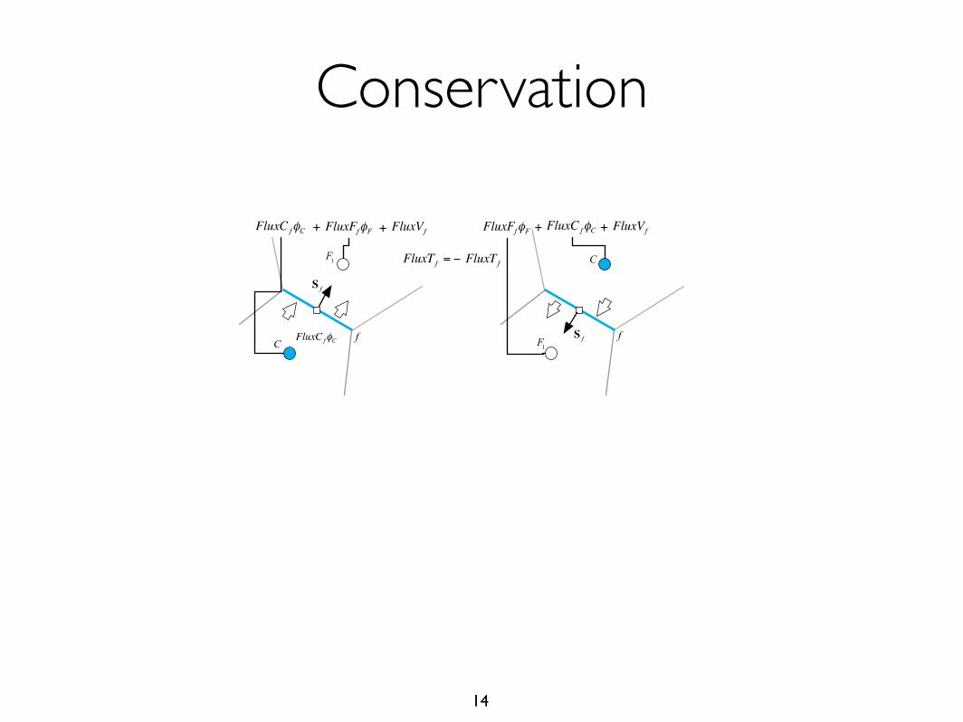
Conservation

14

FluxC fφC

C

F1

f

S f

FluxC fφC

C

F1fS f

FluxTf

FluxFfφF FluxVfFluxC fφC FluxFfφF FluxVf

FluxTf= −

+ + + +

Transportiveness

15

C

Pe = 0 Pe > 0

W E

Other Properties

16

Consistency

Stability

Economy

Boundedness of the Interpolation Profile

Variable Arrangment

Variable Arrangement

18

Cell-centered Vertex-centered

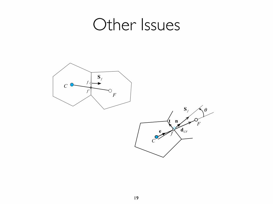
Other Issues

19

f

f’

S f

C

F

S f

n

e dCF

t

θ

C

F

f

Matrix Connectivity

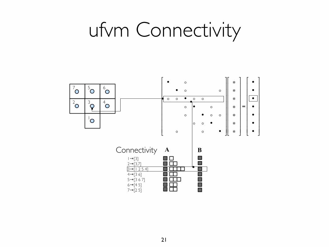
ufvm Connectivity

21

• !• ! !

! ! • ! !! • !! • ! !! ! •

! ! •

!

"

########

$

%

&&&&&&&&

∗∗∗∗∗∗∗

!

"

########

$

%

&&&&&&&&

=

•••••••

!

"

########

$

%

&&&&&&&&

1

2 3 4

5 67

1→[3]2→[3,7]3→[1 2 5 4]4→[3 6]5→[3 6 7]6→[4 5]7→[2 5]

Connectivity A B

OpenFoam Connectivity

22

• !• ! !

! ! • ! !! • !! • ! !! ! •

! ! •

!

"

########

$

%

&&&&&&&&

∗∗∗∗∗∗∗

!

"

########

$

%

&&&&&&&&

=

•••••••

!

"

########

$

%

&&&&&&&&

lduMatrix diag() lower() upper()