02.01.1

Chapter 02.02 Differentiation of Continuous Functions After reading this chapter, you should be able to:

1. derive formulas for approximating the first derivative of a function, 2. derive formulas for approximating derivatives from Taylor series, 3. derive finite difference approximations for higher order derivatives, and 4. use the developed formulas in examples to find derivatives of a function.

The derivative of a function at x is defined as

( ) ( ) ( )x

xfxxfxfx ∆

−∆+=′

→∆ 0lim

To be able to find a derivative numerically, one could make x∆ finite to give,

( ) ( ) ( )x

xfxxfxf∆

−∆+≈′ .

Knowing the value of x at which you want to find the derivative of ( )xf , we choose a value of x∆ to find the value of ( )xf ′ . To estimate the value of ( )xf ′ , three such approximations are suggested as follows. Forward Difference Approximation of the First Derivative From differential calculus, we know

( ) ( ) ( )x

xfxxfxfx ∆

−∆+=′

→∆ 0lim

For a finite x∆ ,

( ) ( ) ( )x

xfxxfxf∆

−∆+≈′

The above is the forward divided difference approximation of the first derivative. It is called forward because you are taking a point ahead of x . To find the value of ( )xf ′ at ixx = , we may choose another point x∆ ahead as 1+= ixx . This gives

( ) ( ) ( )x

xfxfxf iii ∆

−≈′ +1

02.02.2 Chapter 02.02

( ) ( )ii

ii

xxxfxf

−−

=+

+

1

1

where ii xxx −=∆ +1

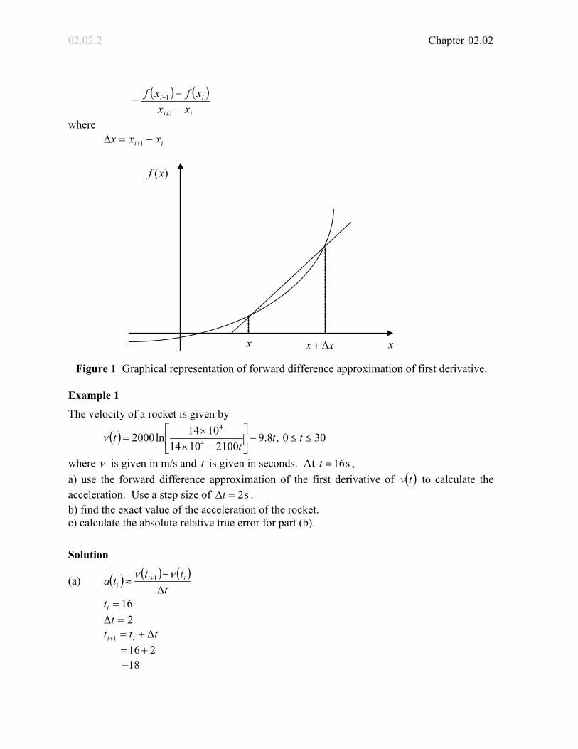
Figure 1 Graphical representation of forward difference approximation of first derivative.

Example 1 The velocity of a rocket is given by

( ) 300 ,8.921001014

1014ln2000 4

4

≤≤−

−×

×= tt

ttν

where ν is given in m/s and t is given in seconds. At s16=t , a) use the forward difference approximation of the first derivative of ( )tν to calculate the acceleration. Use a step size of s2=∆t . b) find the exact value of the acceleration of the rocket. c) calculate the absolute relative true error for part (b). Solution

(a) ( ) ( ) ( )t

ttta iii ∆

−≈ + νν 1

16=it 2Δ =t ttt ii Δ1 +=+ 216+= =18

)(xf

xx ∆+ x x

Continuous Differentiation 02.02.3

( ) ( ) ( )2

161816 νν −≈a

( ) ( ) ( )188.91821001014

1014ln200018 4

4

−

−××

=ν

m/s 02.453=

( ) ( ) ( )168.91621001014

1014ln200016 4

4

−

−××

=ν

m/s 07.392= Hence

( ) ( ) ( )2

161816 νν −≈a

2

07.39202.453 −=

2m/s474.30= (b) The exact value of ( )16a can be calculated by differentiating

( ) tt

t 8.921001014

1014ln2000 4

4

−

−×

×=ν

as

( ) ( )[ ]tνdtdta =

Knowing that

( )[ ]t

tdtd 1ln = and 2

11ttdt

d−=

( ) 8.921001014

10141014

210010142000 4

4

4

4

−

−×

×

×−×

=tdt

dtta

( ) ( ) ( ) 8.9210021001014

101411014

210010142000 24

4

4

4

−−

−×

×−

×−×

=t

t

t

t3200

4.294040+−−−

=

( ) ( )( )163200

164.29404016+−−−

=a

2m/s674.29= (c) The absolute relative true error is

100Value True

Value eApproximatValue True×

−=∈t

02.02.4 Chapter 02.02

100674.29

474.30674.29×

−=

%6967.2= Backward Difference Approximation of the First Derivative We know

( ) ( ) ( )x

xfxxfxfx ∆

−∆+=′

→∆ 0lim

For a finite x∆ ,

( ) ( ) ( )x

xfxxfxf∆

−∆+≈′

If x∆ is chosen as a negative number,

( ) ( ) ( )x

xfxxfxf∆

−∆+≈′

( ) ( )x

xxfxfΔ

Δ−−=

This is a backward difference approximation as you are taking a point backward from x . To find the value of ( )xf ′ at ixx = , we may choose another point x∆ behind as 1−= ixx . This gives

( ) ( ) ( )x

xfxfxf iii ∆

−≈′ −1

( ) ( )1

1

−

−

−−

=ii

ii

xxxfxf

where 1Δ −−= ii xxx

Continuous Differentiation 02.02.5

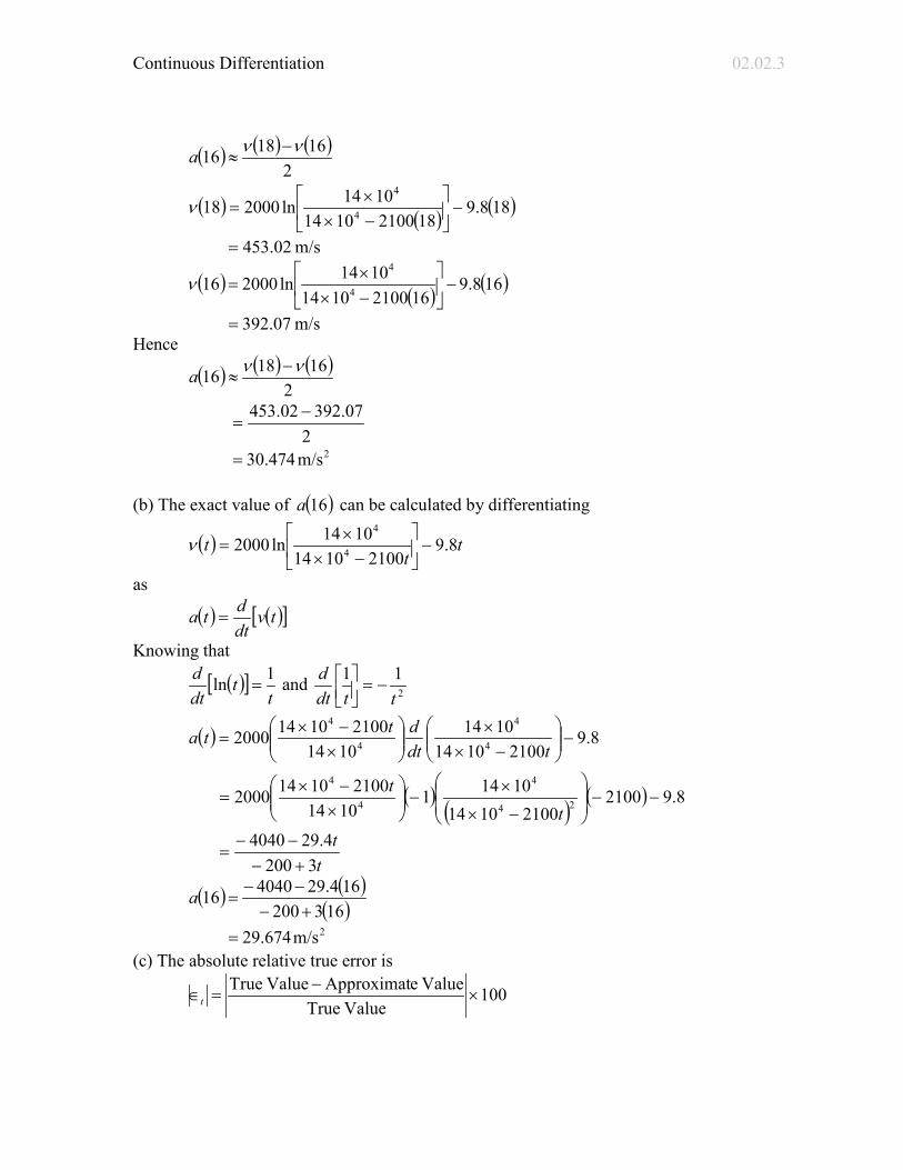
Figure 2 Graphical representation of backward difference approximation of first derivative. Example 2 The velocity of a rocket is given by

( ) 300,8.921001014

1014ln2000 4

4

≤≤−

−×

×= tt

ttν

(a) Use the backward difference approximation of the first derivative of ( )tν to calculate the acceleration at s16=t . Use a step size of s 2=∆t . (b) Find the absolute relative true error for part (a). Solution

( ) ( ) ( )t

ttta ii

∆−

≈ −1νν

16=it 2Δ =t ttt ii Δ1 −=− 216−= = 14

( ) ( ) ( )2

141616 νν −≈a

( ) ( ) ( )168.91621001014

1014ln200016 4

4

−

−××

=ν

m/s07.392=

( ) ( ) ( )148.91421001014

1014ln200014 4

4

−

−××

=ν

)(xf

x xx ∆− x

02.02.6 Chapter 02.02 m/s24.334=

( ) ( ) ( )2

141616 νν −≈a

2

24.33407.392 −=

2m/s 915.28= (b) The exact value of the acceleration at s16=t from Example 1 is ( ) 2m/s 674.2916 =a The absolute relative true error for the answer in part (a) is

100674.29

915.28674.29×

−=∈t

%5584.2= Forward Difference Approximation from Taylor Series

Taylor’s theorem says that if you know the value of a function )(xf at a point ix and all its derivatives at that point, provided the derivatives are continuous between ix and 1+ix , then

( ) ( ) ( )( ) ( ) ( ) +−′′

+−′+= +++2

111 !2 iii

iiiii xxxfxxxfxfxf

Substituting for convenience ii xxx −= +1Δ

( ) ( ) ( ) ( ) ( ) +′′

+′+=+2

1 Δ!2

Δ xxfxxfxfxf iiii

( ) ( ) ( ) ( ) ( ) +∆′′

−∆−

=′ + xxf

xxfxf

xf iiii !2

1

( ) ( ) ( ) ( )xOx

xfxfxf iii ∆+

∆−

=′ +1

The ( )xO ∆ term shows that the error in the approximation is of the order of x∆ . Can you now derive from the Taylor series the formula for the backward divided difference approximation of the first derivative? As you can see, both forward and backward divided difference approximations of the first derivative are accurate on the order of ( )xO ∆ . Can we get better approximations? Yes, another method to approximate the first derivative is called the central difference approximation of the first derivative. From the Taylor series

( ) ( ) ( ) ( ) ( ) ( ) ( ) +′′′

+′′

+′+=+32

1 Δ!3

Δ!2

Δ xxf

xxf

xxfxfxf iiiii (1)

and

( ) ( ) ( ) ( ) ( ) ( ) ( ) +′′′

−′′

+′−=−32

1 Δ!3

Δ!2

Δ xxf

xxf

xxfxfxf iiiii (2)

Subtracting Equation (2) from Equation (1)

Continuous Differentiation 02.02.7

( ) ( ) ( )( ) ( ) ( ) +′′′

+′=− −+3

11 Δ!3

2Δ2 xxfxxfxfxf iiii

( ) ( ) ( ) ( ) ( ) +∆′′′

−∆−

=′ −+ 211

!32x

xfx

xfxfxf iii

i

( ) ( ) ( )211

2xO

xxfxf ii ∆+

∆−

= −+

hence showing that we have obtained a more accurate formula as the error is of the order of ( )2xO ∆ .

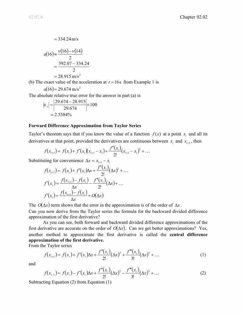
Figure 3 Graphical representation of central difference approximation of first derivative. Example 3 The velocity of a rocket is given by

( ) 300,8.921001014

1014ln2000 4

4

≤≤−

−×

×= tt

ttν .

(a) Use the central difference approximation of the first derivative of ( )tν to calculate the acceleration at s 16=t . Use a step size of s 2=∆t . (b) Find the absolute relative true error for part (a). Solution

( ) ( ) ( )t

ttta iii ∆

−≈ −+

211 νν

16=it 2=∆t

)(xf

xx ∆+ x xx ∆− x

02.02.8 Chapter 02.02

18

2161

=+=∆+=+ ttt ii

14

2161

=−=∆−=− ttt ii

( ) ( ) ( )( )22

141816 νν −≈a

( ) ( )4

1418 νν −=

( ) ( ) ( )188.91821001014

1014ln200018 4

4

−

−××

=ν

m/s02.453=

( ) ( ) ( )148.91421001014

1014ln200014 4

4

−

−××

=ν

m/s24.334=

( ) ( ) ( )4

141816 νν −≈a

4

24.33402.453 −=

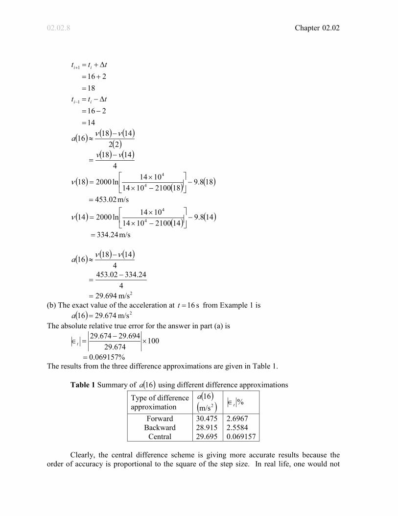
2m/s 694.29= (b) The exact value of the acceleration at s 16=t from Example 1 is ( ) 2m/s 674.2916 =a The absolute relative true error for the answer in part (a) is

100674.29

694.29674.29×

−=∈t

%069157.0= The results from the three difference approximations are given in Table 1.

Table 1 Summary of ( )16a using different difference approximations

Type of difference approximation

( )16a ( )2m/s

%t∈

Forward Backward

Central

30.475 28.915 29.695

2.6967 2.5584 0.069157

Clearly, the central difference scheme is giving more accurate results because the order of accuracy is proportional to the square of the step size. In real life, one would not

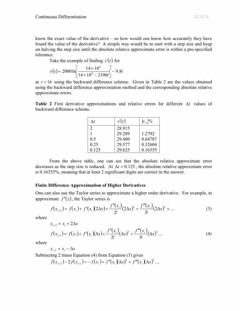
Continuous Differentiation 02.02.9 know the exact value of the derivative – so how would one know how accurately they have found the value of the derivative? A simple way would be to start with a step size and keep on halving the step size until the absolute relative approximate error is within a pre-specified tolerance. Take the example of finding ( )tv′ for

( ) tt

t 8.921001014

1014ln2000 4

4

−

−×

×=ν

at 16=t using the backward difference scheme. Given in Table 2 are the values obtained using the backward difference approximation method and the corresponding absolute relative approximate errors. Table 2 First derivative approximations and relative errors for different t∆ values of backward difference scheme.

t∆ ( )tv′ %a∈ 2 1 0.5 0.25 0.125

28.915 29.289 29.480 29.577 29.625

1.2792 0.64787 0.32604 0.16355

From the above table, one can see that the absolute relative approximate error decreases as the step size is reduced. At 125.0=∆t , the absolute relative approximate error is 0.16355%, meaning that at least 2 significant digits are correct in the answer. Finite Difference Approximation of Higher Derivatives One can also use the Taylor series to approximate a higher order derivative. For example, to approximate ( )xf ′′ , the Taylor series is

( ) ( ) ( )( ) ( ) ( ) ( ) ( ) +′′′

+′′

+′+=+32

2 Δ2!3

Δ2!2

Δ2 xxf

xxf

xxfxfxf iiiii (3)

where xxx ii Δ22 +=+

( ) ( ) ( )( ) ( ) ( ) ( ) ( ) 321 !3!2

xxf

xxf

xxfxfxf iiiii ∆

′′′+∆

′′+∆′+=+ (4)

where xxx ii Δ1 −=− Subtracting 2 times Equation (4) from Equation (3) gives ( ) ( ) ( ) ( )( ) ( )( ) 32

12 ΔΔ2 xxfxxfxfxfxf iiiii ′′′+′′+−=− ++

02.02.10 Chapter 02.02

( ) ( ) ( ) ( )( )

( )( ) +′′′−+−

=′′ ++ xxfx

xfxfxfxf i

iiii Δ

Δ2

212

( ) ( ) ( ) ( )( )

( )xOx

xfxfxfxf iiii ∆+

∆+−

≈′′ ++2

12 2 (5)

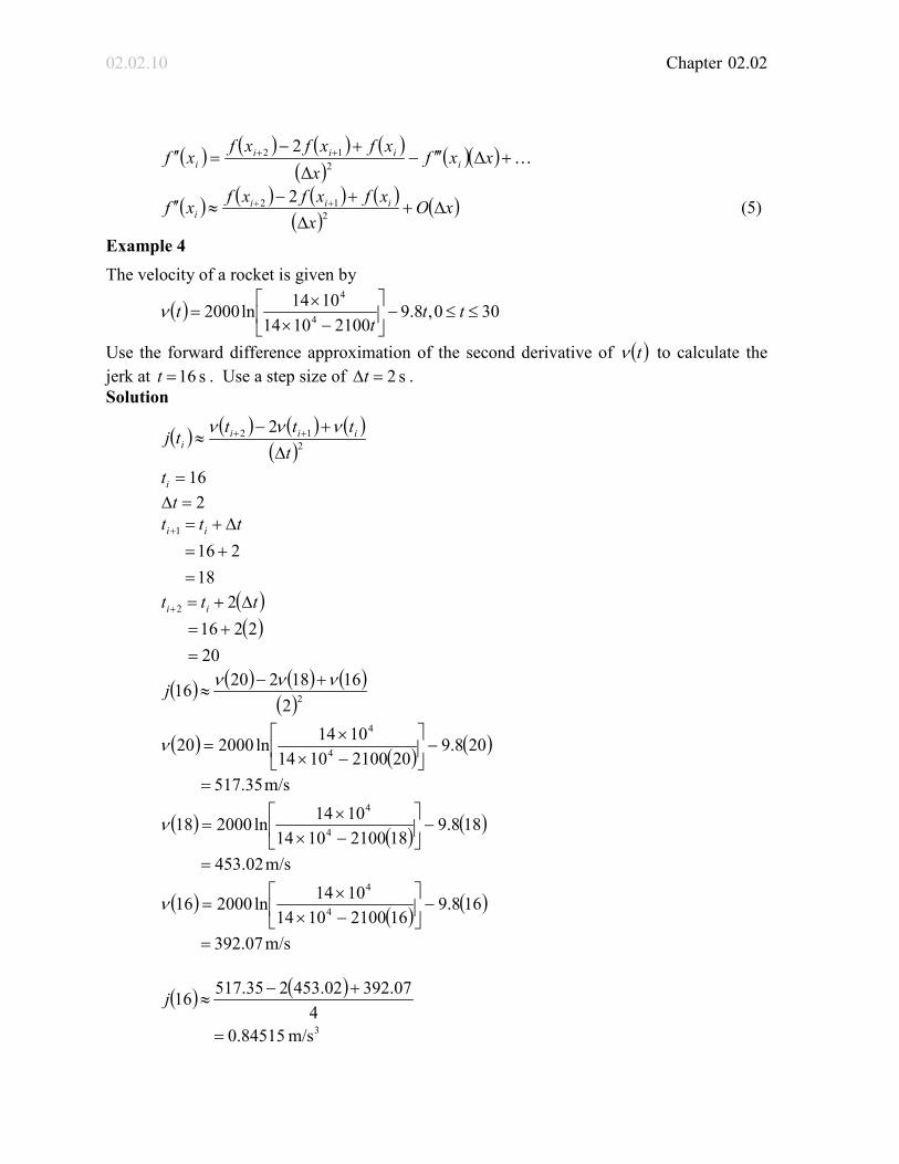
Example 4 The velocity of a rocket is given by

( ) 300,8.921001014

1014ln2000 4

4

≤≤−

−×

×= tt

ttν

Use the forward difference approximation of the second derivative of ( )tν to calculate the jerk at s 16=t . Use a step size of s 2=∆t . Solution

( ) ( ) ( ) ( )( )2

12 2t

ttttj iiii ∆

+−≈ ++ ννν

16=it 2=∆t

18

2161

=+=∆+=+ ttt ii

( )( )

202216

22

=+=

∆+=+ ttt ii

( ) ( ) ( ) ( )( )22

161822016 ννν +−≈j

( ) ( ) ( )208.92021001014

1014ln200020 4

4

−

−××

=ν

m/s35.517=

( ) ( ) ( )188.91821001014

1014ln200018 4

4

−

−××

=ν

m/s02.453=

( ) ( ) ( )168.91621001014

1014ln200016 4

4

−

−××

=ν

m/s07.392=

( ) ( )4

07.39202.453235.51716 +−≈j

3m/s 84515.0=

Continuous Differentiation 02.02.11 The exact value of ( )16j can be calculated by differentiating

( ) tt

t 8.921001014

1014ln2000 4

4

−

−×

×=ν

twice as

( ) ( )[ ]tνdtdta = and

( ) ( )[ ]tadtdtj =

Knowing that

( )[ ]t

tdtd 1ln = and

2

11ttdt

d−=

( ) 8.921001014

10141014

210010142000 4

4

4

4

−

−×

×

×−×

=tdt

dtta

( ) ( ) ( ) 8.9210021001014

101411014

210010142000 24

4

4

4

−−

−×

×−

×−×

=t

t

t

t3200

4.294040+−−−

=

Similarly it can be shown that

( ) ( )[ ]tadtdtj =

2)3200(18000

t+−=

( )

3

2

m/s77909.0 )]16(3200[

1800016

=

+−=j

The absolute relative true error is

10077909.0

84515.077909.0×

−=∈t

%4797.8= The formula given by Equation (5) is a forward difference approximation of the second derivative and has an error of the order of ( )xO ∆ . Can we get a formula that has a better accuracy? Yes, we can derive the central difference approximation of the second derivative. The Taylor series is

02.02.12 Chapter 02.02

( ) ( ) ( ) ( ) ( ) ( ) ( ) ( ) ( ) ...!4!3!2

4321 +∆

′′′′+∆

′′′+∆

′′+∆′+=+ xxfxxfxxfxxfxfxf iii

iii (6)

where xxx ii Δ1 +=+

( ) ( ) ( ) ( ) ( ) ( ) ( ) ( ) ( ) −∆′′′′

+∆′′′

−∆′′

+∆′−=−432

1 !4!3!2xxfxxfxxfxxfxfxf iii

iii (7)

where xxx ii Δ1 −=− Adding Equations (6) and (7), gives

( ) ( ) ( ) ( )( ) ( ) ( ) ...12

24

211 +

∆′′′+∆′′+=+ −+xxfxxfxfxfxf iiiii

( ) ( ) ( ) ( )( )

( )( ) ...12

2 2

211 +

∆′′′′−

∆+−

=′′ −+ xxfx

xfxfxfxf iiiii

( ) ( ) ( )( )

( )2211 2 xO

xxfxfxf iii ∆+

∆+−

= −+

Example 5 The velocity of a rocket is given by

( ) 300 ,8.921001014

1014ln2000 4

4

≤≤−

−×

×= tt

ttν ,

(a) Use the central difference approximation of the second derivative of ( )tν to calculate the jerk at s 16=t . Use a step size of s 2=∆t . Solution The second derivative of velocity with respect to time is called jerk. The second order approximation of jerk then is

( ) ( ) ( ) ( )( )2

11 2t

ttttj iiii ∆

+−≈ −+ ννν

16=it 2=∆t

18

2161

=+=∆+=+ ttt ii

14

2162

=−=∆−=+ ttt ii

( ) ( ) ( ) ( )( )22

141621816 ννν +−≈j

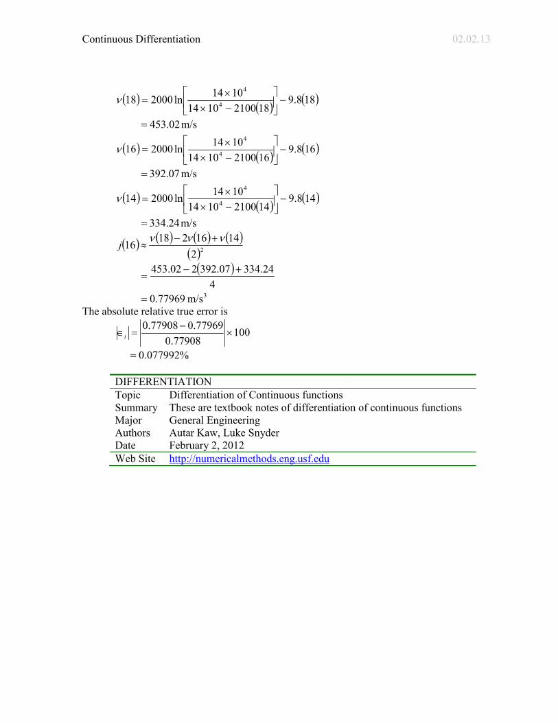
Continuous Differentiation 02.02.13

( ) ( ) ( )188.91821001014

1014ln200018 4

4

−

−××

=ν

m/s02.453=

( ) ( ) ( )168.91621001014

1014ln200016 4

4

−

−××

=ν

m/s07.392=

( ) ( ) ( )148.91421001014

1014ln200014 4

4

−

−××

=ν

m/s24.334=

( ) ( ) ( ) ( )( )22

141621816 ννν +−≈j

( )4

24.33407.392202.453 +−=

3m/s 77969.0= The absolute relative true error is

10077908.0

77969.077908.0×

−=∈t

%077992.0=

DIFFERENTIATION Topic Differentiation of Continuous functions Summary These are textbook notes of differentiation of continuous functions Major General Engineering Authors Autar Kaw, Luke Snyder Date February 2, 2012 Web Site http://numericalmethods.eng.usf.edu