chap13
47
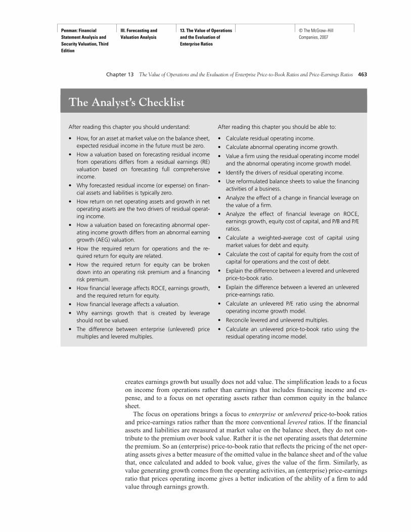
Penman: Financial Statement Analysis and Security Valuation, Third Edition III. Forecasting and Valuation Analysis 13. The Value of Operations and the Evaluation of Enterprise Ratios © The McGraw-Hill Companies, 2007 Link to previous chapter LINKS Part Two of the book showed how to analyze the operating and financing activities of a firm and the profitability and growth they generate. This chapter This chapter develops valuations based only on operating profitability and growth and shows how to calculate intrinsic price-to-book ratios and price-earnings ratios for operations. Link to next chapter Chapter 14 will develop simple forecasting and valuation methods based on the valuation models for operations in this chapter. Link to Web page Apply the methods of this chapter to valuing the operations of firms—visit the text Web Site at www.mhhe.com/penman3e. How can forecasting and valuation be simplified? Can financing activities be ignored in valuation if they do not generate value? What is an "economic profit" valuation model? How are intrinsic price- to-book ratios and intrinsic price-earnings ratios calculated for a firm's operations? Chapter Thirteen The Value of Operations and the Evaluation of Enterprise Price-to- Book Ratios and Price- Earnings Ratios The residual earnings model of Chapter 5 and the abnormal earnings growth model of Chapter 6 give us two ways to value equities from the financial statements: price book values or price earnings. The analysis of financial statements in Part Two of the book provides an understanding of what drives residual earnings and earnings growth. We are now in a position to apply the analysis tools of Part Two to develop valuations using residual earnings and abnormal earnings growth methods. With valuation in mind we want to forecast the aspects of the business that generate value. In Part Two of the book we took pains to distinguish operating activities from financing activities with the understanding that it is operations that generate value. This chapter shows how this distinction is incorporated in developing forecasts for valuation. It shows that if net financial obligations are measured in the balance sheet at market value, financing activities can be ignored in forecasting. You will see that this makes forecasting easier. In particular, complications that arise from the effect of financial leverage on resid- ual earnings, abnormal earnings growth, and the cost of capital can be ignored. You will also see that this protects you from paying too much for earnings growth, for leverage
-
Upload
lauren-webb -
Category
Documents
-
view
15 -
download
1
description
chapter 13 penman
Transcript of chap13
Penman: Financial Statement Analysis and Security Valuation, Third Edition
III. Forecasting and Valuation Analysis
13. The Value of Operations and the Evaluation of Enterprise Ratios
© The McGraw−Hill Companies, 2007
Link to previous chapter
LINKS
Part Two of the bookshowed how to analyze the
operating and financingactivities of a firm
and the profitabilityand growth they generate.
This chapter
This chapter developsvaluations based only on
operating profitability andgrowth and shows how to
calculate intrinsicprice-to-book ratios and
price-earnings ratiosfor operations.
Link to next chapter
Chapter 14 will developsimple forecasting and
valuation methods based onthe valuation models for
operations in this chapter.
Link to Web page
Apply the methods of thischapter to valuing the
operations of firms—visitthe text Web Site at
www.mhhe.com/penman3e.
How arereturns
calculated?
What issustainable
growth?
How canforecasting and
valuation besimplified?
Can financingactivities beignored invaluation ifthey do not
generatevalue?
What is an"economic
profit"valuationmodel?
How areintrinsic price-to-book ratiosand intrinsic
price-earningsratios calculated
for a firm'soperations?
Chapter Thirteen
The Value of Operationsand the Evaluationof Enterprise Price-to-Book Ratios and Price-Earnings Ratios
The residual earnings model of Chapter 5 and the abnormal earnings growth model ofChapter 6 give us two ways to value equities from the financial statements: price bookvalues or price earnings. The analysis of financial statements in Part Two of the bookprovides an understanding of what drives residual earnings and earnings growth. We arenow in a position to apply the analysis tools of Part Two to develop valuations usingresidual earnings and abnormal earnings growth methods.
With valuation in mind we want to forecast the aspects of the business that generatevalue. In Part Two of the book we took pains to distinguish operating activities fromfinancing activities with the understanding that it is operations that generate value. Thischapter shows how this distinction is incorporated in developing forecasts for valuation.It shows that if net financial obligations are measured in the balance sheet at market value,financing activities can be ignored in forecasting. You will see that this makes forecastingeasier. In particular, complications that arise from the effect of financial leverage on resid-ual earnings, abnormal earnings growth, and the cost of capital can be ignored. You willalso see that this protects you from paying too much for earnings growth, for leverage
Penman: Financial Statement Analysis and Security Valuation, Third Edition
III. Forecasting and Valuation Analysis
13. The Value of Operations and the Evaluation of Enterprise Ratios
© The McGraw−Hill Companies, 2007
creates earnings growth but usually does not add value. The simplification leads to a focuson income from operations rather than earnings that includes financing income and ex-pense, and to a focus on net operating assets rather than common equity in the balancesheet.
The focus on operations brings a focus to enterprise or unlevered price-to-book ratiosand price-earnings ratios rather than the more conventional levered ratios. If the financialassets and liabilities are measured at market value on the balance sheet, they do not con-tribute to the premium over book value. Rather it is the net operating assets that determinethe premium. So an (enterprise) price-to-book ratio that reflects the pricing of the net oper-ating assets gives a better measure of the omitted value in the balance sheet and of the valuethat, once calculated and added to book value, gives the value of the firm. Similarly, asvalue generating growth comes from the operating activities, an (enterprise) price-earningsratio that prices operating income gives a better indication of the ability of a firm to addvalue through earnings growth.
Chapter 13 The Value of Operations and the Evaluation of Enterprise Price-to-Book Ratios and Price-Earnings Ratios 463
The Analyst’s Checklist
After reading this chapter you should understand:
• How, for an asset at market value on the balance sheet,expected residual income in the future must be zero.
• How a valuation based on forecasting residual incomefrom operations differs from a residual earnings (RE)valuation based on forecasting full comprehensiveincome.
• Why forecasted residual income (or expense) on finan-cial assets and liabilities is typically zero.
• How return on net operating assets and growth in netoperating assets are the two drivers of residual operat-ing income.
• How a valuation based on forecasting abnormal oper-ating income growth differs from an abnormal earninggrowth (AEG) valuation.
• How the required return for operations and the re-quired return for equity are related.
• How the required return for equity can be brokendown into an operating risk premium and a financingrisk premium.
• How financial leverage affects ROCE, earnings growth,and the required return for equity.
• How financial leverage affects a valuation.
• Why earnings growth that is created by leverageshould not be valued.
• The difference between enterprise (unlevered) pricemultiples and levered multiples.
After reading this chapter you should be able to:
• Calculate residual operating income.
• Calculate abnormal operating income growth.
• Value a firm using the residual operating income modeland the abnormal operating income growth model.
• Identify the drivers of residual operating income.
• Use reformulated balance sheets to value the financingactivities of a business.
• Analyze the effect of a change in financial leverage onthe value of a firm.
• Analyze the effect of financial leverage on ROCE,earnings growth, equity cost of capital, and P/B and P/Eratios.
• Calculate a weighted-average cost of capital usingmarket values for debt and equity.
• Calculate the cost of capital for equity from the cost ofcapital for operations and the cost of debt.
• Explain the difference between a levered and unleveredprice-to-book ratio.
• Explain the difference between a levered an unleveredprice-earnings ratio.
• Calculate an unlevered P/E ratio using the abnormaloperating income growth model.
• Reconcile levered and unlevered multiples.
• Calculate an unlevered price-to-book ratio using theresidual operating income model.

Penman: Financial Statement Analysis and Security Valuation, Third Edition
III. Forecasting and Valuation Analysis
13. The Value of Operations and the Evaluation of Enterprise Ratios
© The McGraw−Hill Companies, 2007
A MODIFICATION TO RESIDUAL EARNINGS FORECASTING: RESIDUAL OPERATING INCOME
Let’s remind ourselves of the residual earnings model for valuing equity:
where
Residual earnings (RE) = Earnings − Required earnings on book value of equity
REt = Earnt − (ρE − 1) CSEt−1
This RE model instructs us to anchor the valuation of equity on the book value of equity,then add value for earnings forecasted in excess of the required earnings on book value,where the required rate of return is the cost of capital for equity, ρE – 1.
We understand from this model that, if an asset is forecasted to earn at its required rateof return, forecasted residual earnings will be zero and the asset will be worth its bookvalue. Correspondingly, if the book value of an asset is equal to its intrinsic value, then theresidual earnings that it is expected to yield will be zero. We can make use of these proper-ties in valuing equities even though the total book value of equity is not equal to its value.If some assets are measured in the balance sheet at market value and if market value equalsintrinsic value, then we know we don’t have to forecast the residual earnings that they willproduce; their forecasted residual earnings are zero. We only have to forecast residual earn-ings from assets not at market value. Accordingly, we can calculate the value of equity as
V0E = CSE0 + Present value of forecasted residual earnings from net assets not at
market value
To carry out this valuation we have to be able to distinguish the earnings from assets orliabilities at market value from those that are not. The income from operating assets is usu-ally earned by using assets jointly, which makes it difficult to identify the income from theseparate assets. However, we have seen that we can usually separate operating income (gen-erated by the net operating assets) from net financial expense (generated by the net finan-cial obligations). And, net financial obligations are typically measured on the balance sheetat market value.
The two components of earnings identified by the reformulation of financial statementsin Part Two of the book are listed in Table 13.1 along with the balance sheet component that
(13.1)VE
E E E
0 0
0 2 3
= +
= + + + +
CSE Present value of forecasted residual earnings
CSERE RE RE1 2 3
ρ ρ ρL
464 Part Three Forecasting and Valuation Analysis
Earnings Component Book Value Component Residual Earnings Measure
Operating income (OI) Net operating assets Residual operating income: (NOA) OIt – (ρF – 1) NOAt–1
Net financial expense (NFE) Net financial obligations Residual net financial expense:(NFO) NFEt – (ρD – 1) NFOt–1
Earnings Common stockholders’ Residual earnings:equity (CSE) Earn1 – (ρE – 1) CSEt–1
TABLE 13.1Components ofEarnings and BookValue, andCorrespondingResidual EarningsMeasures
Penman: Financial Statement Analysis and Security Valuation, Third Edition
III. Forecasting and Valuation Analysis
13. The Value of Operations and the Evaluation of Enterprise Ratios
© The McGraw−Hill Companies, 2007
Chapter 13 The Value of Operations and the Evaluation of Enterprise Price-to-Book Ratios and Price-Earnings Ratios 465
generates them. Beside each component is the corresponding residual earnings measure.To get the residual earnings measure, each income component is matched with the corre-sponding balance sheet component and charged with the required earnings rate (the cost ofcapital) for the component. We will discuss the cost of capital in the next section but fornow recognize that the required return for the different sources of income depends on theriskiness of that activity. Note that ρD is 1 plus the cost of capital for net debt (or, as it maybe, the required return on net financial assets), and ρF is 1 plus the cost of capital for oper-ating activities. In all cases the residual earnings is earnings in excess of the earnings (orexpense) required for the asset (or liability) in the balance sheet to be earning at the rele-vant cost of capital.
Residual earnings from net operating assets is residual operating income, and we willrefer to it as ReOI:
Residual operating income = Operating income (after tax) − Required income on net operating assets
ReOIt = OIt − (ρF − 1)NOAt−1
Residual operating income charges the operating income with a charge for using the netoperating assets. Residual operating income is also referred to as “economic profit” or“economic value added,” and some consulting firms have taken these terms as trademarksfor their valuation products. For Nike, with after-tax operating income of $1,035 million in2004 and net operating assets at the beginning of the year of $4,330 million, the residualoperating income for 2004 was ReOI2004 = $1,035 − (0.086 × 4,330) = $662.6 million for arequired return of 8.6 percent. For Reebok, with an after-tax operating income of $237 mil-lion in 2004 and net operating assets at the beginning of the year of $731 million, ReOI2004 =$237 − (0.090 × 731) = $171.2 million for a required return of 9.0 percent.
Similarly, residual earnings from the net financial obligations is residual net financialexpense, ReNFE = NFEt − (ρD − 1)NFOt−1, or, if the firm has net financial assets, residualnet financial income. Thus residual net financial expense is net financial expense less therequired cost of the net debt.
With forecasts of ReOI and ReNFE, we can value the NOA and NFO. The value of thenet financial obligations, V0
NFO, that mature at some time T in the future is
Value of NFO = NFO + Present value of expected residual net financial expense
(13.2)
If the NFO are measured at market value, it must be that forecasted ReNFE are zero: For$100 million of debt at an interest rate of 5 percent, interest expense is $5 million andReNFE = $5 − (0.05 × 100) = 0. Thus, V0
NFO = NFO. The book value of the net financialobligations is their value.
The value of the net operating assets, V0NOA, for a going concern is
Value of operations = Net operating assets + Present value of expected residual operating income
(13.3)VF F F
T
FT
T
FT
0 01 2
2
3
3NOA NOA
OI OI OI
OI CV
= + + + + +
+
Re Re Re
Re
ρ ρ ρ
ρ ρ
L
VD D D
T
DT0
2
2 3NFO 1 3NFO +
NFE NFE NFE NFE= + + + +Re Re Re Re
ρ ρ ρ ρL

Penman: Financial Statement Analysis and Security Valuation, Third Edition
III. Forecasting and Valuation Analysis
13. The Value of Operations and the Evaluation of Enterprise Ratios
© The McGraw−Hill Companies, 2007
466 Part Three Forecasting and Valuation Analysis
That is, the value is the book value of the NOA, plus the present value of expected residualoperating income from these assets to a forecast horizon, plus a continuing value that is thevalue of expected residual operating income after the horizon. This model is the same formas the residual income model but applies to the net operating assets instead of the commonshareholders’ equity. Continuing values summarize the analyst’s expectation of a firm’s per-formance beyond a forecast horizon. Continuing values can be calculated at a point wherethe analyst forecasts that performance will follow a regular pattern.
Corresponding to the three cases for the residual earnings model in Chapter 5, the con-tinuing value for the residual operating income model can take three forms:
In Case 1 we expect residual operating income (ReOI) to be zero after the forecast hori-zon because we expect the net operating assets to earn at the cost of capital. In Case 2 weexpect ReOI to be at a constant, permanent level, and in Case 3 we expect ReOI to growperpetually at the rate g. The analyst’s task, then, is to forecast the level and growth of resid-ual operating income at the forecast horizon.
The value of the operations is also called the value of the firm. It is also sometimes referredto as enterprise value. The value of the equity is V0
E = V0NOA – V0
NFO. So if the NFO are mea-sured at market value on the balance sheet—that is, expected residual net financial expenses(ReNFE) are zero—then (recognizing that NOA – NFO = CSE) the value of the equity is
Value of common equity = Book value of common equity (13.4)+ Present value of expected residual operating income
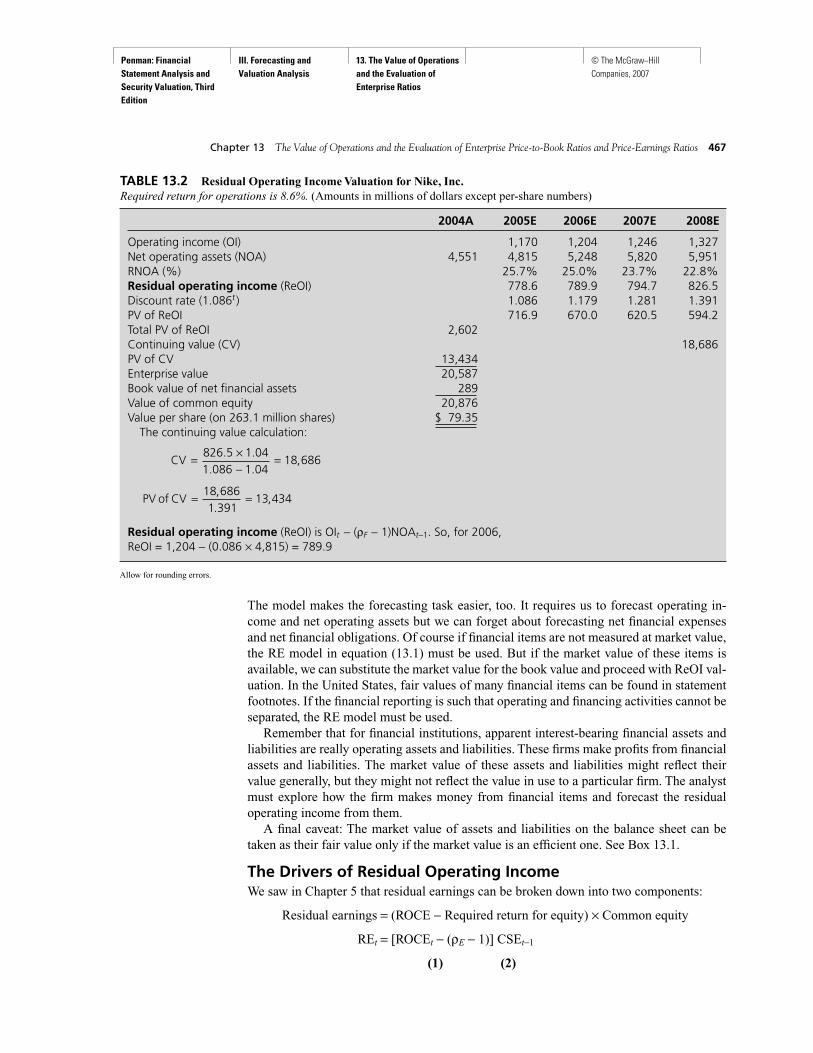
This model is the residual operating income model.Table 13.2 values Nike using the model. The forecasts are for operating income and net
operating assets, not total earnings and common shareholders’ equity; the financing compo-nents of the income statement and the balance sheet are ignored. The forecasts imply the re-turn on net operating assets (RNOA) numbers indicated, with declining profitability up to2008, as is common. Residual operating income, calculated as described at the bottom ofthe table, is forecasted to grow after 2008 at the 4 percent average GDP growth rate. With thecontinuing value implied by this growth rate, the value of the operations in early 2005—theenterprise value—is $20,587 million and the value of the equity (that includes Nike’s 2004net financial assets) is $20,876 million, or $79.35 per share. Nike’s shares traded at $75 atthe time, so one could view the pro forma here as one that is (approximately) consistent withthe forecasts implied by the market price. We might then ask whether this pro forma (thatjustifies the current market price) is a reasonable one. If, through analysis, we forecastedhigher residual operating income in the future, we would conclude that Nike is underpriced,given we accepted the 8.6 percent required return as reasonable.
The residual operating income model makes sense. If debt and financial assets are zeroresidual earnings producers, then they add no value to their recorded value. We are goingto get the valuation by forecasting the profitability of the operations that do add value.
V SEE
F F F
T
FT
T
FT0 0
1 2
2
3
3= + + + + + +C
OI OI OI OI CVRe Re Re Re
ρ ρ ρ ρ ρL
Case 1: CV
Case 2: CVOI
Case 3: CVOI
T
TT
F
TT
F g
=
=−
=−
+
+
0
11
1
Re
Re
ρ
ρ
Penman: Financial Statement Analysis and Security Valuation, Third Edition
III. Forecasting and Valuation Analysis
13. The Value of Operations and the Evaluation of Enterprise Ratios
© The McGraw−Hill Companies, 2007
The model makes the forecasting task easier, too. It requires us to forecast operating in-come and net operating assets but we can forget about forecasting net financial expensesand net financial obligations. Of course if financial items are not measured at market value,the RE model in equation (13.1) must be used. But if the market value of these items isavailable, we can substitute the market value for the book value and proceed with ReOI val-uation. In the United States, fair values of many financial items can be found in statementfootnotes. If the financial reporting is such that operating and financing activities cannot beseparated, the RE model must be used.
Remember that for financial institutions, apparent interest-bearing financial assets andliabilities are really operating assets and liabilities. These firms make profits from financialassets and liabilities. The market value of these assets and liabilities might reflect theirvalue generally, but they might not reflect the value in use to a particular firm. The analystmust explore how the firm makes money from financial items and forecast the residualoperating income from them.
A final caveat: The market value of assets and liabilities on the balance sheet can betaken as their fair value only if the market value is an efficient one. See Box 13.1.
The Drivers of Residual Operating IncomeWe saw in Chapter 5 that residual earnings can be broken down into two components:
Residual earnings = (ROCE − Required return for equity) × Common equity
REt = [ROCEt − (ρE − 1)] CSEt−1
(1) (2)
Chapter 13 The Value of Operations and the Evaluation of Enterprise Price-to-Book Ratios and Price-Earnings Ratios 467
2004A 2005E 2006E 2007E 2008E
Operating income (OI) 1,170 1,204 1,246 1,327Net operating assets (NOA) 4,551 4,815 5,248 5,820 5,951RNOA (%) 25.7% 25.0% 23.7% 22.8%Residual operating income (ReOI) 778.6 789.9 794.7 826.5Discount rate (1.086t ) 1.086 1.179 1.281 1.391PV of ReOI 716.9 670.0 620.5 594.2Total PV of ReOI 2,602Continuing value (CV) 18,686PV of CV 13,434Enterprise value 20,587Book value of net financial assets 289Value of common equity 20,876Value per share (on 263.1 million shares) $ 79.35
The continuing value calculation:
Residual operating income (ReOI) is OIt − (ρF − 1)NOAt−1. So, for 2006, ReOI = 1,204 − (0.086 × 4,815) = 789.9
Allow for rounding errors.
PV of CV = =18 6861 391
13 434,.
,
CV = ×−
=826 5 1 041 086 1 04
18 686. .
. .,
TABLE 13.2 Residual Operating Income Valuation for Nike, Inc.Required return for operations is 8.6%. (Amounts in millions of dollars except per-share numbers)
Penman: Financial Statement Analysis and Security Valuation, Third Edition
III. Forecasting and Valuation Analysis
13. The Value of Operations and the Evaluation of Enterprise Ratios
© The McGraw−Hill Companies, 2007
We referred to the two components, ROCE and book values, as residual earningsdrivers: RE is driven by the amount of shareholders’ investment and the rate of return onthis investment relative to the cost of equity capital. Residual operating income can simi-larly be broken down into two components:
Residual operating income = (RNOA – Required return for operations) × Net operating assets
ReOIt = [RNOAt – (ρF – 1)] NOAt–1
(1) (2)
The two components of ReOI are RNOA and net operating assets and we refer to these asresidual operating income drivers: ReOI is driven by the amount of net operating assets putin place and the profitability of those assets relative to the cost of capital. The valuation ofNike in Table 13.2 involved forecasts of RNOA, as indicated, and growth in net operatingassets. The combination produces growing residual operating income.
Residual net financial expense (or income) also can be broken down into two drivers:
Residual net financial expense = (Net borrowing cost – Cost of net debt) × Net debt
ReNFEt = [NBCt – (ρD – 1)] NFOt–1
So ReNFE is driven by the amount of net financial debt and the net borrowing cost relativeto the cost of debt. For a firm that issues debt for financing, expected borrowing costs areequal to the cost of the debt. So no matter how much debt is put in place, no value is addedthrough the two drivers, and expected ReNFE is zero.
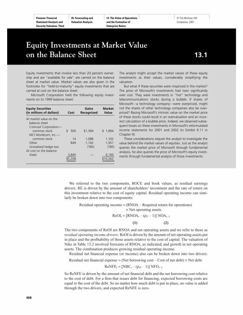
The analyst might accept the market values of these equityinvestments as their values, considerably simplifying thevaluation.
But what if these securities were mispriced in the market?The price of Microsoft’s investments had risen significantlyover cost. They were investments in “hot” technology andtelecommunications stocks during a bubble. If shares ofMicrosoft—a technology company—were overpriced, mightnot the shares of other technology companies also be over-priced? Basing Microsoft’s intrinsic value on the market priceof these stocks could result in an overvaluation and an incor-rect calculation of a bubble price. Indeed, we observed subse-quent losses on these investments in Microsoft’s reformulatedincome statements for 2001 and 2002 (in Exhibit 9.11 inChapter 9).
These considerations require the analyst to investigate thevalue behind the market values of equities. Just as the analystqueries the market price of Microsoft through fundamentalanalysis, he also queries the price of Microsoft’s equity invest-ments through fundamental analysis of those investments.
Equity Investments at Market Value on the Balance Sheet 13.1
Equity investments that involve less than 20 percent owner-ship and are “available for sale” are carried on the balancesheet at market value. Market values are also given in thefootnotes for “held-to-maturity” equity investments that arecarried at cost on the balance sheet.
Microsoft Corporation held the following equity invest-ments on its 1999 balance sheet:
Equity Securities Gains Market (in millions of dollars) Cost Recognized Value
At market value on the balance sheetComcast Corporation—
common stock $ 500 $1,394 $ 1,894MCI Worldcom, Inc.—
common stock 14 1,088 1,102Other 849 1,102 1,951Unrealized hedge loss (785) (785)
At cost on the balancesheet 3,845 — 6,100
$5,208 $10,262
468
Penman: Financial Statement Analysis and Security Valuation, Third Edition
III. Forecasting and Valuation Analysis
13. The Value of Operations and the Evaluation of Enterprise Ratios
© The McGraw−Hill Companies, 2007
Rather, value is added to book value through the operations, and our breakdown tellsus that this is done by earning an RNOA that is greater than the cost of capital for opera-tions and by putting investments in place to earn at this rate. Accordingly, forecasting in-volves forecasting the two drivers, future RNOA and future NOA. We will see how theseforecasts are developed in the next two chapters.
A MODIFICATION TO ABNORMAL EARNINGS GROWTH FORECASTING:ABNORMAL GROWTH IN OPERATING INCOME
Let us remind ourselves of the abnormal earnings growth model for valuing equity:
V0E = Capitalized [Forward earnings + Present value of abnormal earnings growth]
(13.5)
where
Abnormal earnings growtht (AEG) = Cum-dividend earningst − Normal earningst
= [Earningst + (ρE – 1)dt−1] − ρEEarningst−1
= [Gt − ρE] × Earningst−1
where Gt is the cum-dividend earnings growth rate for the period. The AEG model instructsus to forecast forward (one-year ahead) earnings, then add value for subsequent cum-dividend earnings forecasted in excess of earnings growing at the required rate of return forequity. Forecasted earnings include earnings from reinvesting dividends, for a firm deliverstwo sources of earnings, one from earnings within the firm and the other from earnings thatcan be earned from reinvesting dividends paid by the firm. We understand from this modelthat earnings growth in itself does not add value, only abnormal growth over the requiredgrowth. If abnormal earnings growth is expected to be zero, the equity will be worth justthe capitalized value of its forward earnings.
Consider now where abnormal growth comes from. Growth does not come from financ-ing activities. To see this, refer back to the prototype savings account in Chapter 6 whereabnormal earnings growth is always zero. Debt investments and debt obligations work justlike a savings account: Debt is always expected to earn (or incur expenses) at the requiredreturn on the debt so, adjusting for any cash paid on the debt (the “dividend” from debt),net financial expense can grow only at a rate equal to the required return. To see it anotherway, we have just recognized that, if the net financial obligations are at market value on thebalance sheet, residual income from the financing activities is expected to be zero. So thechange in residual income, period-to-period, is also expected to be zero, and abnormalearnings growth is always equal to the change in residual income.
Abnormal earnings growth is generated by operations. This makes sense for, once again,it is the operations that add value. As the financing activities do not contribute to growthover the required return, we focus on abnormal growth in operating income.
Abnormal Growth in Operating Income and the “Dividend”from Operating ActivitiesWhen introducing earnings growth in Chapter 6, we recognized that growth in (ex-dividend) earnings—the growth that analysts typically forecast—is not the growth that weshould focus on. Earnings growth rates will be lower the more dividends are paid, but
=−
+ + + +⎡
⎣⎢
⎤
⎦⎥
1
12 3
2
4
3ρ ρ ρ ρE E E E
EarnAEG AEG AEG
1 L
Chapter 13 The Value of Operations and the Evaluation of Enterprise Price-to-Book Ratios and Price-Earnings Ratios 469

Penman: Financial Statement Analysis and Security Valuation, Third Edition
III. Forecasting and Valuation Analysis
13. The Value of Operations and the Evaluation of Enterprise Ratios
© The McGraw−Hill Companies, 2007
dividends can be reinvested to earn more, adding to growth. So any analysis of growth mustfocus on cum-dividend earnings growth. In focusing on growth in the operating incomecomponent of earnings, we also must not make the mistake of focusing on growth in oper-ating income if cash that otherwise could be reinvested in operations is paid out of theoperations. Dividends are net cash payments to shareholders out of earnings (that they canreinvest). What is the cash paid out of operations (that can be reinvested elsewhere)? Whatare the “dividends” from the operating activities?
Our depiction of business activities in Chapter 7 supplies the answer to this question.Look at Figure 7.3, which summarizes business activities, and Figure 7.4, which summa-rizes how those activities are represented in reformulated financial statements. Net divi-dends, d, are the dividends from the financing activities to the shareholders. Net paymentsto bondholders and debt issuers, F, are the “dividends” from the financing activities tothese claimants. But the “dividend” from the operating activities to the financing activitiesis the free cash flow. Business works as follows: Operations pay a dividend to the financingactivities—in the form of free cash flow—and the financing activities apply this cash to paydividends to the outside claimants. Indeed, the reformulated cash flow statement is a state-ment that reports the cash dividend from the operating activities (free cash flow) and howthat dividend is divided among cash to debtholders and cash to shareholders in the financ-ing activities: C − I = d + F.
Accordingly, abnormal operating income growth is calculated as:
Abnormal operating income growtht (AOIG)
= Cum-dividend operating incomet – Normal operating incomet
= [Operating incomet + (ρF – 1)FCFt–1] − ρF Operating incomet–1
where free cash flow (FCF) is, of course, cash from operations minus cash investment(C − I). Compare this measure to abnormal earnings growth (AEG) above. Operating in-come is substituted for earnings and free cash flow is substituted for dividends. And, as theincome is from operations, the required return that defines normal growth is the requiredreturn for operations. A firm delivers abnormal operating income growth if growth in op-erating income—cum-dividend, after reinvesting free cash flow—is greater than the normalgrowth rate required for operations.
Just as AEG can be expressed in terms of cum-dividend growth rates relative to therequired rate, so can abnormal operating income growth:
Abnormal operating income growtht (AOIG) = [Gt – ρF] × Operating incomet–1
where Gt is now the cum-dividend operating income growth rate rather than earnings.Table 13.3 lays out the abnormal earnings growth measures that correspond to the oper-
ating and financing components of earnings, in a similar way to the residual earnings
470 Part Three Forecasting and Valuation Analysis
Earnings Component Abnormal Earnings Growth Measure
Operating income (OI) Abnormal operating income growth:[OIt + (ρF – 1)FCFt–1] – ρFOIt–1
[Gt – ρF] × OIt–1
Net financing expense (NFE) Abnormal net financial expense growth:[NFEt + (ρD – 1)Ft–1] – ρDNFEt–1
Earnings Abnormal earnings growth:[Earnt + (ρE – 1)dt–1] – ρEEarnt–1
[GtE – ρE] × Earnt–1
TABLE 13.3EarningsComponents andCorrespondingAbnormal EarningsGrowth Measures
Penman: Financial Statement Analysis and Security Valuation, Third Edition
III. Forecasting and Valuation Analysis
13. The Value of Operations and the Evaluation of Enterprise Ratios
© The McGraw−Hill Companies, 2007
breakdown in Table 13.1. A calculation for abnormal growth in net financial expense is in-cluded there, for completeness, but (like residual net financing expense) it is not a measurewe will make use of because it is expected to be zero. (Note, for completeness, that the“dividend” for debt financing is the cash payment to debtholders, F.)
With an understanding of abnormal growth in operating income, we can lay out an ab-normal operating income growth model to value the equity. Forecasting abnormal operat-ing income growth yields the value of the operations, just as forecasting residual operatingincome yields the value of the operations. Subtracting the value of the net financial obliga-tions yields the value of the equity and, if net financial obligations are measured at marketvalue on the balance sheet, the book value suffices for their value. So,
Value of common equity = Capitalized [Forward operating income + Present value of abnormal operating income growth] – Net financial obligations
(13.6)
You see that this is the same form as the AEG model (equation 13.5) except that operatingincome is substituted for earnings, and the cost of capital for the operations is substitutedfor the equity cost of capital. Like the ReOI model, this AOIG model simplifies the valua-tion task, for we need only forecast operating income and can ignore the financing aspectsof future earnings. As the model values the enterprise or the firm before deducting the netfinancial obligations, the model (like the ReOI model) is referred to as an enterprise valu-ation model or a valuation model for the firm.
Table 13.4 applies the model to valuing Nike, as in Table 13.2. The layout is the same asthat for the abnormal earnings growth valuations in Chapter 6. As with the ReOI model,operating income and net operating assets are forecasted, but the net operating asset fore-casts are then applied to forecast free cash flows: C – I = OI – ∆NOA, as in the Method 1calculation in Chapter 10. Free cash flow does not have to be forecasted in addition to theother forecasts—it is calculated directly from those forecasts. Expected abnormal operat-ing income growth is calculated from forecasts of operating income and free cash flow, asdescribed at the bottom of the table, and those forecasts are converted to a valuation asprescribed by the model. Note that, just as AEG is always equal to the change in residualearnings (RE), AOIG is equal to the change in ReOI in each period (in Table 13.2). Thevaluation is, of course, the same as that obtained using ReOI methods.
THE COST OF CAPITAL AND VALUATION
Step 4 of fundamental analysis combines forecasts from Step 3 with the cost of capital toget a valuation. The preceding models have shown how this is done, but now we have en-countered three costs of capital: the cost of capital for equity, ρE; the cost of capital for debt,ρD; and the cost of capital for operations, ρF. These need a little explanation. We will notcalculate them here but note that this is done using the beta technologies discussed in theappendix to Chapter 3, which are covered in corporate finance texts. (We will discuss howfundamental risk affects the cost of capital in Chapter 18.) Here you should be sure youhave a good appreciation of the concepts, because with this understanding, forecasting and
VE
F F F F0
2 3
2
4
3
0
1
1=
−+ + + +
⎡
⎣⎢
⎤
⎦⎥
−
ρ ρ ρ ρOI
AOIG AOIG AOIG
NFO
1 L
Chapter 13 The Value of Operations and the Evaluation of Enterprise Price-to-Book Ratios and Price-Earnings Ratios 471

Penman: Financial Statement Analysis and Security Valuation, Third Edition
III. Forecasting and Valuation Analysis
13. The Value of Operations and the Evaluation of Enterprise Ratios
© The McGraw−Hill Companies, 2007
valuation can be simplified. We will see that, just as residual income can be broken downinto operating and financing components, so can the equity cost of capital. And we will seehow the financing element of the cost of equity capital can be ignored in valuation.
The Cost of Capital for OperationsResidual earnings is earnings for the equity holders and so is calculated and discountedusing the cost of capital for equity, ρE. Residual operating income is earnings for theoperations and so is calculated and discounted using a cost of capital for the operations, ρF.
472 Part Three Forecasting and Valuation Analysis
2004A 2005E 2006E 2007E 2008E
Operating income (OI) 1,170 1,204 1,246 1,327Net operating assets (NOA) 4,551 4,815 5,248 5,820 5,951Free cash flow (C − I = OI − ∆NOA) 906 771 674 1,196Income from reinvested free cash flow (at 8.6%) 77.9 66.3 58.0Cum-dividend OI 1,281.9 1312.3 1385.0Normal OI 1,270.6 1,307.5 1,353.2Abnormal OI Growth (AOIG) 11.3 4.8 31.8Discount rate 1.086 1.179 1.281PV of AOIG 10.4 4.1 24.8Total PV of AOIG 39.3Continuing value 719PV of continuing value 561.3Forward OI for 2005 1,170.0
1,770.6Capitalization rate 0.086Enterprise value 20,587Book value of net financial assets 289Value of common equity 20,876Value per share (on 263.1 million shares) $ 79.35Cum-dividend growth rate in OI 9.57% 9.00% 11.16%The continuing value calculation:
Income from reinvested free cash flow is prior year’s free cash flow earning at the required return of 8.6%. So,for 2006, income from reinvested free cash flow is 0.086 × 906 = 77.9.
Cum-dividend OI is operating income plus income from reinvesting free cash flow. So, for 2006, cum-dividend OIis 1,204 + 77.9 = 1,281.9.
Normal OI is prior years’ operating income growing at the required return. So, for 2006, normal OI is 1,170 ×1.086 = 1,270.6.
Abnormal OI growth (AOIG) is cum-dividend OI minus normal OI. So, for 2006, AOIG is 1,281.9 − 1,270.6 = 11.3.AOIG is also given by OIt−1 × (Gt − ρF). So, for 2006, AOIG is (1.0957 − 1.086) × 1,170 = 11.3.
Allow for rounding errors.
PV of CV = =719 01 281
561 3.
..
CV = ×−
=31 8 1 041 086 1 04
719 0. .
. ..
TABLE 13.4 Abnormal Operating Income Growth Valuation for Nike, Inc.Required return for operations is 8.6%.(Amounts in millions of dollars except per-share number)
Penman: Financial Statement Analysis and Security Valuation, Third Edition
III. Forecasting and Valuation Analysis
13. The Value of Operations and the Evaluation of Enterprise Ratios
© The McGraw−Hill Companies, 2007
Payoffs must be discounted at a rate that reflects their risk and the risk for the operationsmay be different from the risk for equity. The risk in the operations is referred to as opera-tional risk or firm risk. Operational risk arises from factors that may hurt operating prof-itability. The sensitivity of sales and operating expenses to recessions and other shocks de-termines the operating risk. Airlines have relatively high operating risk because people flyless during recessions and fuel costs are subject to shocks in oil prices. The required returnthat compensates for this risk is called the cost of capital for operations or the cost of cap-ital for the firm. This is what we have labeled ρF (where F is for “firm”).
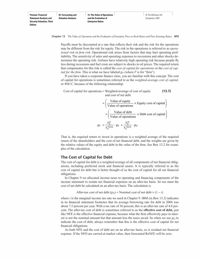
If you have taken a corporate finance class, you are familiar with this concept. The costof capital for operations is sometimes referred to as the weighted-average cost of capital,or WACC, because of the following relationship:
Cost of capital for operations = Weighted-average of cost of equity (13.7)and cost of net debt
That is, the required return to invest in operations is a weighted average of the requiredreturn of the shareholders and the cost of net financial debt, and the weights are given bythe relative values of the equity and debt in the value of the firm. See Box 13.2 for exam-ples of the calculation.
The Cost of Capital for DebtThe cost of capital for debt is a weighted average of all components of net financial oblig-ations, including preferred stock and financial assets. It is typically referred to as thecost of capital for debt but is better thought of as the cost of capital for all net financialobligations.
In Chapter 9 we allocated income taxes to operating and financing components of theincome statement to restate net financial expenses on an after-tax basis. So too must thecost of net debt be calculated on an after-tax basis. The calculation is
After-tax cost of net debt (ρD) = Nominal cost of net debt × (1 − t)
where t is the marginal income tax rate we used in Chapter 9. IBM (in Box 13.2) indicatesin its financial statement footnotes that its average borrowing rate for debt in 2004 wasabout 7.5 percent per year. With a tax rate of 36 percent, this is an after-tax rate of 4.8 per-cent. The after-tax cost of debt is sometimes referred to as the effective cost of debt, justlike NFE is the effective financial expense, because what the firm effectively pays in inter-est is not the nominal amount but that amount less the taxes saved. So when we use ρD toindicate the cost of debt, always remember that this is the effective cost of capital for netfinancial obligations.
As both NFE and the cost of debt are on an after-tax basis, so is residual net financialexpense. If the NFO are carried at market value, then forecasted ReNFE will be zero.
= ×⎛⎝⎜
⎞⎠⎟
+ ×⎛⎝⎜
⎞⎠⎟
= ⋅ + ⋅
Value of equity
Value of operationsEquity cost of capital
Value of debt
Value of operationsDebt cost of capital
NOA NOAρ ρ ρF
E
E
D
DV
V
V
V0
0
0
0
Chapter 13 The Value of Operations and the Evaluation of Enterprise Price-to-Book Ratios and Price-Earnings Ratios 473

Penman: Financial Statement Analysis and Security Valuation, Third Edition
III. Forecasting and Valuation Analysis
13. The Value of Operations and the Evaluation of Enterprise Ratios
© The McGraw−Hill Companies, 2007
Operating Risk, Financing Risk, and the Cost of Equity CapitalThe calculation of the WACC in equation (13.7) is a bit misleading because it looks as if thecost of capital for operations is determined by the costs of debt and equity. The operationshave their inherent risk, and this depends on the riskiness of the business and not on howthe business is financed. Thus a standard notion in finance—another Modigliani and Millerconcept—states that the cost of capital for the firm is unaffected by the amount of debt orequity in the financing of the operational assets. Rather than the required return for opera-tions being determined by the cost of capital for equity and debt, the return that equity anddebt investors require is determined by the riskiness of the operations. The operations havetheir interest risk, and this is imposed on the equity holders and the debtholders. The wayto think about it is to see the cost of equity determined by the following formula. This is justa rearrangement of the WACC calculation (equation 13.7), putting the equity cost of capitalon the left-hand side rather than the cost of capital for operations:
IBM Dell Nike Reebok
Equity beta 1.7 1.5 0.8 0.9Equity cost of capital 13.0% 12.0% 8.5% 9.0%Cost of capital for debt
(after tax) 4.8% 3.2% 3.2% 3.2%
Market value of equity 135,100 98,200 19,733 2,429Net financial obligations 12,410 (4,130) (289) (23)Market value of operations 147,510 94,070 19,444 2,406
Cost of capital foroperations 12.3% 12.4% 8.6% 9.0%
For IBM, with net financial obligations, the cost of capital foroperations is less than that for equity, while for Dell, Nike, andReebok with net financial assets, the cost of capital for opera-tions is greater than that for equity. For a given level of oper-ating risk, holding (low-risk) financial assets makes the equitycost of capital lower than if the firm borrows.
The WACC calculation for IBM:
The WACC calculation for Dell enters the net financial assetsas negative debt:
The calculation comes with a warning. See Box 13.3.
98 20094 070
12 04 130
94 0703 2 12 39
,,
. %,,
. % . %×⎛⎝⎜
⎞⎠⎟
+ − ×⎛⎝⎜
⎞⎠⎟
=
135 100147 510
13 012 410147 510
4 8 12 31,,
. %,,
. % . %×⎛⎝⎜
⎞⎠⎟
+ ×⎛⎝⎜
⎞⎠⎟
=
The Cost of Capital for Operations: IBM, Dell, Nike, and Reebok 13.2
The cost of capital for operations (also referred to as the costof capital for the firm) is calculated as the weighted average ofthe cost of capital for equity and the (after-tax) cost of capitalfor the net debt (the net financial obligations). Accordingly, itis often called the weighted-average cost of capital (WACC).The calculation is done in two steps:
1. Apply an asset pricing model such as the capital asset pric-ing model (CAPM) to estimate the equity cost of capital.For the CAPM, the inputs are the risk-free rate, the firm’sequity beta, and the market risk premium. See the appen-dix to Chapter 3.
2. Apply the WACC formula 13.7 to convert the equity costof capital to the cost of capital for the operations. Theweights are determined, in principle, by the (intrinsic) valueof the operations and the value of the net financial obliga-tions. As the value of the equity is unknown, the marketvalue of the equity is typically used. The book value of thenet financial obligations approximate their value.
Here are the calculations for four firms, IBM, Dell, Nike, andReebok for 2005 when the 10-year Treasury rate was 4.5 per-cent and the market risk premium was deemed to be 5 percent.Equity beta estimates are those supplied by beta services. Thecost of capital for debt is itself a weighted average of theinterest rates on the various components of net debt and is as-certained from the debt footnote and the yield on financialassets. The rates for Dell, Nike, and Reebok are yields on theirnet financial assets. The market value of operations is the mar-ket value of equity plus the book value of the net financialobligations. (Market values are in millions of dollars.)
474

Penman: Financial Statement Analysis and Security Valuation, Third Edition
III. Forecasting and Valuation Analysis
13. The Value of Operations and the Evaluation of Enterprise Ratios
© The McGraw−Hill Companies, 2007
Required return for equity = Required return for operations (13.8)+ (Market leverage × Required return spread)
(1) (2)
For IBM (in Box 13.2), the cost of equity capital is 12.3% + [12,410/135,100 × (12.3% –4.8%)] = 13.0%. Just as the payoff to shareholders has two components, operating and fi-nancing, the required return to investing for those payoffs has two components, operatingrisk and financing risk components. Component 1 is the risk the operations impose on theshareholder, and the return this requires is the cost of capital for the operations. If the firmhas no net debt, the cost of equity capital is equal to the cost of capital for the operations,that is, ρE = ρF. If IBM had no net debt, the shareholders would require a return of 12.3 per-cent, according to the CAPM calculations. This is sometimes referred to as the case of thepure equity firm. But if there are financing activities, component 2 comes into play; this isthe additional required return for equity due to financing risk. As you can see, this premiumfor financing risk depends on the amount of debt relative to equity (the financial leverage)and the spread between the cost of capital for operations and that for debt. This makessense. Financing risk arises because of leverage and the possibility of that leverage turningunfavorable. Leverage is unfavorable when the return from operations is less than the costof debt, so the equity is more risky the more debt there is and the riskier the operations arerelative to the cost of debt. In Box 13.2, the CAPM required return for operations is lowerfor IBM than for Dell. But the equity investors require a higher return for IBM than for Dellbecause of IBM’s higher leverage. So the financing risk premium is 0.7 percent for IBM(13.0% – 12.3%) and a negative 0.4 percent for Dell (12.0% − 12.4%) because Dell hasnegative leverage.
The leverage here is measured with the values of the debt and equity; it is referred to asmarket leverage to distinguish it from the book leverage (FLEV) discussed in Chapter 11.
If the firm has net financial assets rather than net debt (as with Dell),
Cost of equity captial = Weighted-average of cost of capital for operations (13.9)and required return on net financial assets
where ρNFA is the required return (yield to maturity) on the net financial assets. As financialassets are typically less risky than operations, the cost of equity capital is typically less thanthe cost of capital for the operations in this case. As an exercise, express this in the form ofequation 13.8.
Box 13.3 provides a warning about using cost of capital estimates in fundamentalanalysis.
FINANCING RISK AND RETURN AND THE VALUATION OF EQUITYLeverage and Residual Earnings ValuationYou will have noticed that the expression for the required return for equity in equation(13.8) has a similar form to the expression for the drivers of ROCE in Chapter 11. Bothformulas are below, so you can compare them:
ρ ρ ρE E F
NFA
E NFAV
V
V
V= ⋅ + ⋅0
0
0
0
NOA
ρ ρ ρ ρE F
D
E F DV
V= + −0
0
( )
Chapter 13 The Value of Operations and the Evaluation of Enterprise Price-to-Book Ratios and Price-Earnings Ratios 475

Penman: Financial Statement Analysis and Security Valuation, Third Edition
III. Forecasting and Valuation Analysis
13. The Value of Operations and the Evaluation of Enterprise Ratios
© The McGraw−Hill Companies, 2007
Speculating about the Cost of Capital 13.3
A basic tenant of fundamental analysis (introduced in Chap-ter 1) dictates that the analyst should always be careful todistinguish what she knows from speculation about whatshe doesn’t know. Fundamental analysis is done to challengespeculative stock prices, so it must avoid incorporating specu-lation in any calculation. Unfortunately, standard cost-of-capital measures are speculative, so they must be handledwith care. The appendix to Chapter 3 explained that, despitethe elegant asset pricing models at hand, we really do nothave a sound method to estimate the cost of capital.
SPECULATION ABOUT THE EQUITY RISK PREMIUMCost of capital measures that use the capital asset pricingmodel—like those in Box 13.2—require an estimate of themarket risk premium. We used 5 percent, but estimatesrange, in texts and academic research, from 3.0 percent to9.2 percent. With such a range, IBM’s equity cost of capital(with a beta of 1.7) would range from 9.6 percent to20.1 percent.
The truth is that the equity risk premium is a guess; it is aspeculative number. Add to this the uncertainty as to what theactual beta is, and we have a highly speculative number forthe cost of capital. Building this speculative number into avaluation results in a speculative valuation.
USING SPECULATIVE PRICES IN WEIGHTED-AVERAGE COST OF CAPITAL CALCULATIONSWe have warned against incorporating (possibly speculative)stock prices in a valuation. Thus, we warned of speculativepension fund gains in earnings in Chapter 12 and, in thischapter in Box 13.1, we warned about relying on (possiblyspeculative) equity prices on the balance sheet.
The WACC calculation in equation (13.7) weights equityand debt costs of capital by their respective (intrinsic) values.The standard practice is to use market values instead of intrin-sic values in the weighting, as in the calculations in Box 13.2.This is done under the assumption that market prices are effi-cient. But we carry out fundamental valuations to questionwhether market prices are indeed efficient. If we build inpossibly inefficient prices into our calculation, we compromiseour ability to challenge those prices.
Indeed, you can see that the WACC calculation in equa-tion (13.7) is circular: We wish to estimate the cost of capitalin order to estimate equity value, but the estimate requiresthat we know the equity value! We need methods to breakthis circularity—without reference to speculative marketprices. We turn to this problem in Chapter 18.
As with all instances where we have uncertainty, we get afeel for how that uncertainty affects valuations with sensitivityanalysis. Sensitivity analysis is a feature of the cost of capitalanalysis of Chapter 18, and also of the pro forma analysis thatleads to valuation in Chapter 15.
476
Return on common equity = Return on net operating assets + (Book leverage × Operating spread)
Required return for equity = Required return for operations + (Market leverage × Required return spread)
The equity return in both cases is driven by the return on operating activities plus a pre-mium for financing activities, where the latter is given by the financial leverage and thespread. The only difference is that the second equation refers to required returns rather thanaccounting returns and the leverage is market leverage rather than book leverage.
The comparison is insightful. Leverage increases the ROCE (and thus residual earnings)if the spread is positive, as we saw in Chapter 11. This is the “good news” aspect of leverage.But at the same time leverage increases the required return to equity because of the
ρ ρ ρ ρE F
D
F F DV
V= + −0
0
( )
ROCE RNOA +NFO
CSERNOA NBC= × −
⎡
⎣⎢
⎤
⎦⎥( )
Penman: Financial Statement Analysis and Security Valuation, Third Edition
III. Forecasting and Valuation Analysis
13. The Value of Operations and the Evaluation of Enterprise Ratios
© The McGraw−Hill Companies, 2007
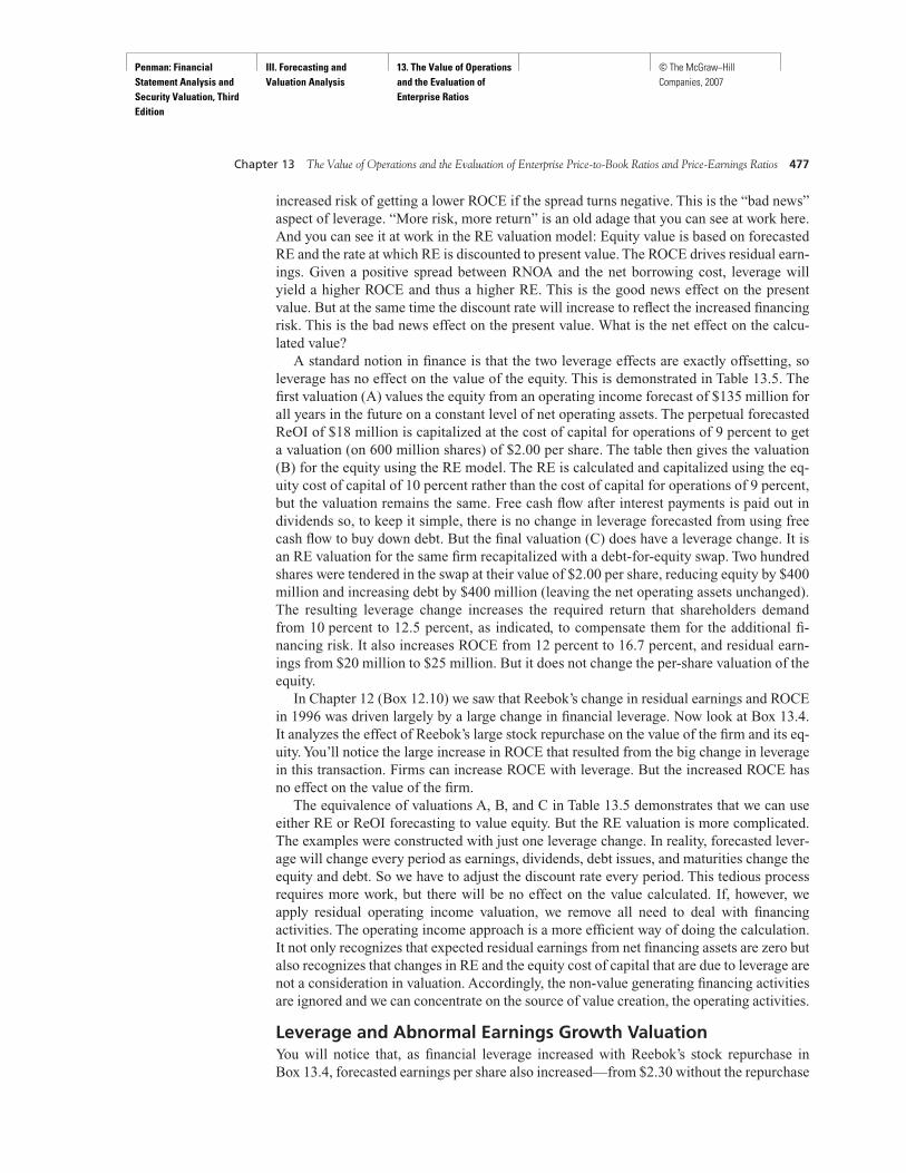
increased risk of getting a lower ROCE if the spread turns negative. This is the “bad news”aspect of leverage. “More risk, more return” is an old adage that you can see at work here.And you can see it at work in the RE valuation model: Equity value is based on forecastedRE and the rate at which RE is discounted to present value. The ROCE drives residual earn-ings. Given a positive spread between RNOA and the net borrowing cost, leverage willyield a higher ROCE and thus a higher RE. This is the good news effect on the presentvalue. But at the same time the discount rate will increase to reflect the increased financingrisk. This is the bad news effect on the present value. What is the net effect on the calcu-lated value?
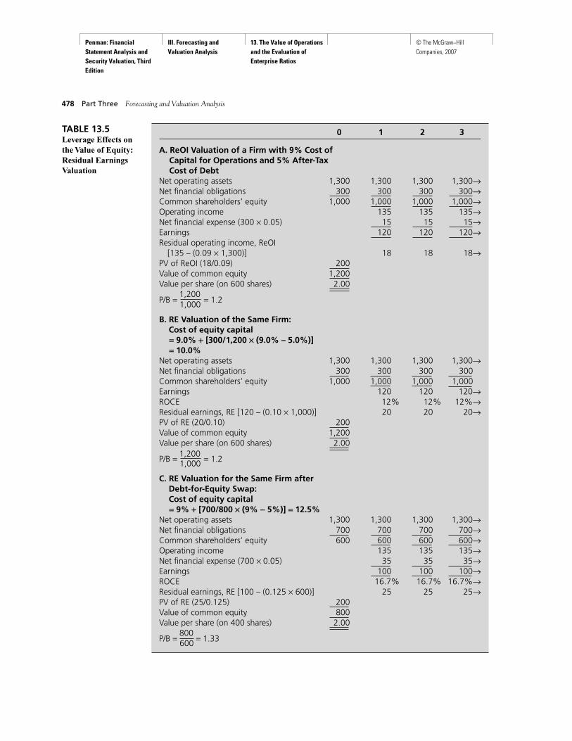
A standard notion in finance is that the two leverage effects are exactly offsetting, soleverage has no effect on the value of the equity. This is demonstrated in Table 13.5. Thefirst valuation (A) values the equity from an operating income forecast of $135 million forall years in the future on a constant level of net operating assets. The perpetual forecastedReOI of $18 million is capitalized at the cost of capital for operations of 9 percent to geta valuation (on 600 million shares) of $2.00 per share. The table then gives the valuation(B) for the equity using the RE model. The RE is calculated and capitalized using the eq-uity cost of capital of 10 percent rather than the cost of capital for operations of 9 percent,but the valuation remains the same. Free cash flow after interest payments is paid out individends so, to keep it simple, there is no change in leverage forecasted from using freecash flow to buy down debt. But the final valuation (C) does have a leverage change. It isan RE valuation for the same firm recapitalized with a debt-for-equity swap. Two hundredshares were tendered in the swap at their value of $2.00 per share, reducing equity by $400million and increasing debt by $400 million (leaving the net operating assets unchanged).The resulting leverage change increases the required return that shareholders demandfrom 10 percent to 12.5 percent, as indicated, to compensate them for the additional fi-nancing risk. It also increases ROCE from 12 percent to 16.7 percent, and residual earn-ings from $20 million to $25 million. But it does not change the per-share valuation of theequity.
In Chapter 12 (Box 12.10) we saw that Reebok’s change in residual earnings and ROCEin 1996 was driven largely by a large change in financial leverage. Now look at Box 13.4.It analyzes the effect of Reebok’s large stock repurchase on the value of the firm and its eq-uity. You’ll notice the large increase in ROCE that resulted from the big change in leveragein this transaction. Firms can increase ROCE with leverage. But the increased ROCE hasno effect on the value of the firm.
The equivalence of valuations A, B, and C in Table 13.5 demonstrates that we can useeither RE or ReOI forecasting to value equity. But the RE valuation is more complicated.The examples were constructed with just one leverage change. In reality, forecasted lever-age will change every period as earnings, dividends, debt issues, and maturities change theequity and debt. So we have to adjust the discount rate every period. This tedious processrequires more work, but there will be no effect on the value calculated. If, however, weapply residual operating income valuation, we remove all need to deal with financingactivities. The operating income approach is a more efficient way of doing the calculation.It not only recognizes that expected residual earnings from net financing assets are zero butalso recognizes that changes in RE and the equity cost of capital that are due to leverage arenot a consideration in valuation. Accordingly, the non-value generating financing activitiesare ignored and we can concentrate on the source of value creation, the operating activities.
Leverage and Abnormal Earnings Growth ValuationYou will notice that, as financial leverage increased with Reebok’s stock repurchase inBox 13.4, forecasted earnings per share also increased—from $2.30 without the repurchase
Chapter 13 The Value of Operations and the Evaluation of Enterprise Price-to-Book Ratios and Price-Earnings Ratios 477
Penman: Financial Statement Analysis and Security Valuation, Third Edition
III. Forecasting and Valuation Analysis
13. The Value of Operations and the Evaluation of Enterprise Ratios
© The McGraw−Hill Companies, 2007
478 Part Three Forecasting and Valuation Analysis
0 1 2 3
A. ReOI Valuation of a Firm with 9% Cost of Capital for Operations and 5% After-Tax Cost of Debt
Net operating assets 1,300 1,300 1,300 1,300→Net financial obligations 300 300 300 300→Common shareholders’ equity 1,000 1,000 1,000 1,000→Operating income 135 135 135→Net financial expense (300 × 0.05) 15 15 15→Earnings 120 120 120→Residual operating income, ReOI
[135 – (0.09 × 1,300)] 18 18 18→PV of ReOI (18/0.09) 200Value of common equity 1,200Value per share (on 600 shares) 2.00
1,200P/B = 1,000 = 1.2
B. RE Valuation of the Same Firm:Cost of equity capital= 9.0% + [300/1,200 ë (9.0% – 5.0%)] = 10.0%
Net operating assets 1,300 1,300 1,300 1,300→Net financial obligations 300 300 300 300Common shareholders’ equity 1,000 1,000 1,000 1,000Earnings 120 120 120→ROCE 12% 12% 12%→Residual earnings, RE [120 – (0.10 × 1,000)] 20 20 20→PV of RE (20/0.10) 200Value of common equity 1,200Value per share (on 600 shares) 2.00
1,200P/B = 1,000 = 1.2
C. RE Valuation for the Same Firm after Debt-for-Equity Swap: Cost of equity capital= 9% + [700/800 ë (9% - 5%)] = 12.5%
Net operating assets 1,300 1,300 1,300 1,300→Net financial obligations 700 700 700 700→Common shareholders’ equity 600 600 600 600→Operating income 135 135 135→Net financial expense (700 × 0.05) 35 35 35→Earnings 100 100 100→ROCE 16.7% 16.7% 16.7%→Residual earnings, RE [100 – (0.125 × 600)] 25 25 25→PV of RE (25/0.125) 200Value of common equity 800Value per share (on 400 shares) 2.00
800P/B = 600 = 1.33
TABLE 13.5Leverage Effects onthe Value of Equity:Residual EarningsValuation
Penman: Financial Statement Analysis and Security Valuation, Third Edition
III. Forecasting and Valuation Analysis
13. The Value of Operations and the Evaluation of Enterprise Ratios
© The McGraw−Hill Companies, 2007
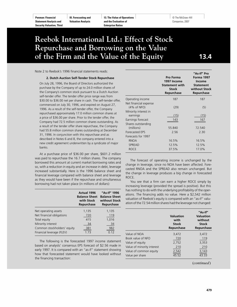
Reebok International Ltd.: Effect of Stock Repurchase and Borrowing on the Value of the Firm and the Value of the Equity 13.4
Note 2 to Reebok’s 1996 financial statements reads:
2. Dutch Auction Self-Tender Stock Repurchase
On July 28, 1996, the Board of Directors authorized thepurchase by the Company of up to 24.0 million shares ofthe Company’s common stock pursuant to a Dutch Auctionself-tender offer. The tender offer price range was from$30.00 to $36.00 net per share in cash. The self-tender offer,commenced on July 30, 1996, and expired on August 27,1996. As a result of the self-tender offer, the Companyrepurchased approximately 17.0 million common shares ata price of $36.00 per share. Prior to the tender offer, theCompany had 72.5 million common shares outstanding. Asa result of the tender offer share repurchase, the Companyhad 55.8 million common shares outstanding at December31, 1996. In conjunction with this repurchase and asdescribed in Notes 6 and 8, the company entered into anew credit agreement underwritten by a syndicate of majorbanks.
At a purchase price of $36.00 per share, $601.2 millionwas paid to repurchase the 16.7 million shares. The companyborrowed this amount at current market borrowing rates andso, with a reduction in equity and an increase in debt, leverageincreased substantially. Here is the 1996 balance sheet andfinancial leverage compared with balance sheet and leverageas they would have been if the repurchase and simultaneousborrowing had not taken place (in millions of dollars):
Actual 1996 “As-If” 1996 Balance Sheet Balance Sheet
with Stock without StockRepurchase Repurchase
Net operating assets 1,135 1,135Net financial obligations 720 119Total equity 415 1,016Minority interest 34 34Common stockholders’ equity 381 982Financial leverage (FLEV) 1.73 0.12
The following is the forecasted 1997 income statementbased on analysts’ consensus EPS forecast of $2.56 made inearly 1997. It is compared with an “as-if” statement showinghow that forecasted statement would have looked withoutthe financing transaction:
“As-If” ProPro Forma Forma 1997
1997 Income Income Statement with Statement
Stock without Stock Repurchase Repurchase
Operating income 187 187Net financial expense
(4% of NFO) (29) (5)Minority interest in
earnings (15) (15)Earnings forecast 143 167 Shares outstanding
(millions) 55.840 72.540Forecasted EPS 2.56 2.30Forecasts for 1997
RNOA 16.5% 16.5%SPREAD 12.5% 12.5%ROCE 37.5% 17.0%
The forecast of operating income is unchanged by thechange in leverage, since no NOA have been affected. Fore-casted RNOA and the SPREAD also remain unchanged. Butthe change in leverage produces a big change in forecastedROCE.
You see that a firm can earn a higher ROCE simply byincreasing leverage (provided the spread is positive). But thishas nothing to do with the underlying profitability of the oper-ations. The financing adds no value. Here a $2,542 millionvaluation of Reebok’s equity is compared with an “as-if” valu-ation of the 72.54 million shares had the leverage not changed:
“As-If”Valuation Valuation
with withoutStock Stock
Repurchase Repurchase
Value of NOA 3,472 3,472Book value of NFO 720 119Value of equity 2,752 3,353Value of minority interest 210 210Value of common equity 2,542 3,143Value per share 45.52 43.33
479
(continued)
Penman: Financial Statement Analysis and Security Valuation, Third Edition
III. Forecasting and Valuation Analysis
13. The Value of Operations and the Evaluation of Enterprise Ratios
© The McGraw−Hill Companies, 2007
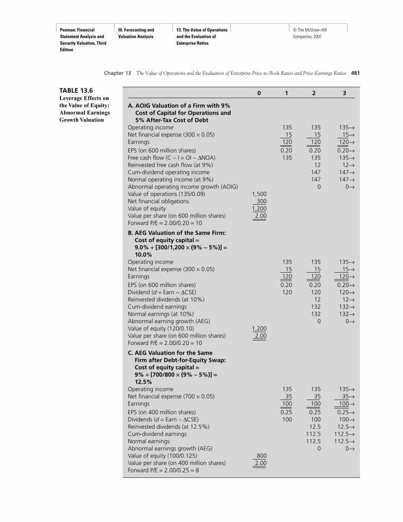
to $2.56 after the repurchase. Just as financial leverage increases ROCE (provided thespread is positive), financial leverage also increases earnings per share. An increase inleverage along with a stock repurchase increases earnings per share even more. With ab-normal earnings growth valuation, we have said that we should pay more for earningsgrowth. But should we pay for EPS growth that comes from leverage? Table 13.6 showsthat the answer is no.
This table applies abnormal earnings growth methods to the same firm as in Table 13.5.The first valuation (A) applies the AOIG model of this chapter. As net operating assets donot change, free cash flow is the same as operating income, and cum-dividend operatingincome (after reinvesting free cash flow) is forecasted to equal normal operating income.Thus abnormal operating income growth from Year 2 onward is forecasted to be zero and,accordingly, the value of the operations is equal to forward operating income ($135 mil-lion) capitalized at the required return for operations of 9 percent, or $1,500 million. Thevalue of the equity, after subtracting net financial obligations, is $1,200, or $2.00 per share,the same valuation (of course) as that using ReOI methods.
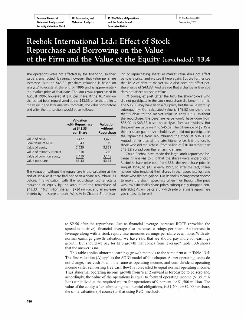
The operations were not affected by the financing, so theirvalue is unaffected. It seems, however, that value per shareincreased. But the $45.52 per-share valuation is based onanalysts’ forecasts at the end of 1996 and is approximatelythe market price at that date. The stock was repurchased inAugust 1996, however, at $36 per share. If the 16.7 millionshares had been repurchased at the $43.33 price that reflectsthe value in the later analysts’ forecasts, the valuations beforeand after the transaction would be as follows:
Valuationwith Repurchase Valuation
at $43.33 withoutper Share Repurchase
Value of NOA 3,472 3,472Book value of NFO 843 119Value of equity 2,629 3,353Value of minority interest 210 210Value of common equity 2,419 3,143Value per share 43.33 43.33
The valuation without the repurchase is the valuation at theend of 1996 as if there had not been a share repurchase, asbefore. The valuation with the repurchase just reflects areduction of equity by the amount of the repurchase of$43.33 × 16.7 million shares = $724 million, and an increasein debt by the same amount. We saw in Chapter 3 that issu-
ing or repurchasing shares at market value does not affectper-share price, and we see it here again. But we further seethat issue of debt at market value also does not affect per-share value of $43.33. And we see that a change in leveragedoes not affect per-share value.
Of course, ex post (after the fact) the shareholders whodid not participate in the stock repurchase did benefit from it.The $36.00 may have been a fair price, but the value went upsubsequently: Our calculated value is $45.52 per share andthat is close to the market value in early 1997. Withoutthe repurchase, the per-share value would have gone from$36.00 to $43.33 based on analysts’ forecast revisions. Butthe per-share value went to $45.52. The difference of $2.19 isthe per-share gain to shareholders who did not participate inthe repurchase from repurchasing the stock at $36.00 inAugust rather than at the later higher price. It is the loss tothose who did repurchase (from selling at $36.00 rather than$43.33) spread over the remaining shares.
Could Reebok have made the large stock repurchase be-cause its analysis told it that the shares were underpriced?Reebok’s share price rose from $36, the repurchase price inAugust 1996, to $43 in early 1997, so after the fact, share-holders who tendered their shares in the repurchase lost andthose who did not gained. Did Reebok’s management chooseto make the stock repurchase when they thought the pricewas low? (Reebok’s share prices subsequently dropped con-siderably.) Again, be careful which side of a share repurchaseyou choose to be on!
480
Reebok International Ltd.: Effect of Stock Repurchase and Borrowing on the Value of the Firm and the Value of the Equity (concluded) 13.4
Penman: Financial Statement Analysis and Security Valuation, Third Edition
III. Forecasting and Valuation Analysis
13. The Value of Operations and the Evaluation of Enterprise Ratios
© The McGraw−Hill Companies, 2007
Chapter 13 The Value of Operations and the Evaluation of Enterprise Price-to-Book Ratios and Price-Earnings Ratios 481
TABLE 13.6Leverage Effects onthe Value of Equity:Abnormal EarningsGrowth Valuation
0 1 2 3
A. AOIG Valuation of a Firm with 9%Cost of Capital for Operations and5% After-Tax Cost of Debt
Operating income 135 135 135→Net financial expense (300 × 0.05) 15 15 15→Earnings 120 120 120→EPS (on 600 million shares) 0.20 0.20 0.20→Free cash flow (C − I = OI − ∆NOA) 135 135 135→Reinvested free cash flow (at 9%) 12 12→Cum-dividend operating income 147 147→Normal operating income (at 9%) 147 147→Abnormal operating income growth (AOIG) 0 0→Value of operations (135/0.09) 1,500Net financial obligations 300Value of equity 1,200Value per share (on 600 million shares) 2.00Forward P/E = 2.00/0.20 = 10
B. AEG Valuation of the Same Firm:Cost of equity capital =9.0% + [300/1,200 ë (9% - 5%)] =10.0%
Operating income 135 135 135→Net financial expense (300 × 0.05) 15 15 15→Earnings 120 120 120→EPS (on 600 million shares) 0.20 0.20 0.20→Dividend (d = Earn − ∆CSE) 120 120 120→Reinvested dividends (at 10%) 12 12→Cum-dividend earnings 132 132→Normal earnings (at 10%) 132 132→Abnormal earning growth (AEG) 0 0→Value of equity (120/0.10) 1,200Value per share (on 600 million shares) 2.00Forward P/E = 2.00/0.20 = 10
C. AEG Valuation for the SameFirm after Debt-for-Equity Swap:Cost of equity capital =9% + [700/800 ë (9% - 5%)] =12.5%
Operating income 135 135 135→Net financial expense (700 × 0.05) 35 35 35→Earnings 100 100 100→EPS (on 400 million shares) 0.25 0.25 0.25→Dividends (d = Earn − ∆CSE) 100 100 100→Reinvested dividends (at 12.5%) 12.5 12.5→Cum-dividend earnings 112.5 112.5→Normal earnings 112.5 112.5→Abnormal earnings growth (AEG) 0 0→Value of equity (100/0.125) 800Value per share (on 400 million shares) 2.00Forward P/E = 2.00/0.25 = 8
Penman: Financial Statement Analysis and Security Valuation, Third Edition
III. Forecasting and Valuation Analysis
13. The Value of Operations and the Evaluation of Enterprise Ratios
© The McGraw−Hill Companies, 2007
Valuation (B) applies an AEG valuation rather than an AOIG valuation. Thus earningsand reinvested dividends are the focus rather than operating income and free cash flows.There is full payout, so dividends are the same as earnings. Now, however, the cost of eq-uity capital is 10.0 percent, so abnormal earnings growth after the first year is forecasted tobe zero. Therefore, the value of the equity is forward earnings of $120 million capitalizedat 10 percent, or $1,200 as before. Value per share is $2.00, which is forward EPS of $0.20capitalized at 10 percent.
Valuation (C) is after the same debt-for-equity swap as in Table 13.5. The change inleverage decreases earnings (as there is now more interest expense with the same operat-ing income) but increases EPS to $0.25. The valuation shows that this increase in eps doesnot change the per-share value of the equity, for the cost of equity capital increases to12.5 percent as a result of the increase in leverage to offset the increase in EPS. The equityvalue—forward EPS of $0.25 capitalized at a cost of equity capital of 12.5 percent—is$2.00, unchanged.
This example confirms that we can use either AEG or AOIG valuation methods toprice earnings growth. But it also suggests that we are better off using AOIG methodsthat focus on the growth from operations. In practice, leverage changes each period so, ifwe were to use AEG valuation, we would have to change the equity cost of capital eachperiod. It is easier to ignore the leverage and focus on the operations. Indeed, financingactivities do not generate abnormal earnings growth, so why complicate the valuation (witha changing cost of capital from changing leverage) when leverage does not produceabnormal earnings growth?
Ignoring financing activities makes sense if you understand that a firm can’t makemoney by issuing bonds at fair market value: These transactions are zero-NPV (and zero-ReNFE). If you forecast that a firm will issue bonds in the future and thus change itsleverage—and the bond issue will be zero-NPV—current value cannot be affected. Simi-larly, an increase in debt to finance a stock repurchase cannot affect value if the stockrepurchase is also at fair market value.
Leverage Creates Earnings GrowthThe example in Table 13.6 provides a warning: Beware of earnings growth that is createdby leverage. Leverage produces earnings growth, but not abnormal earnings growth. So thegrowth created by leverage is not to be valued. See Box 13.5 for a full explanation.
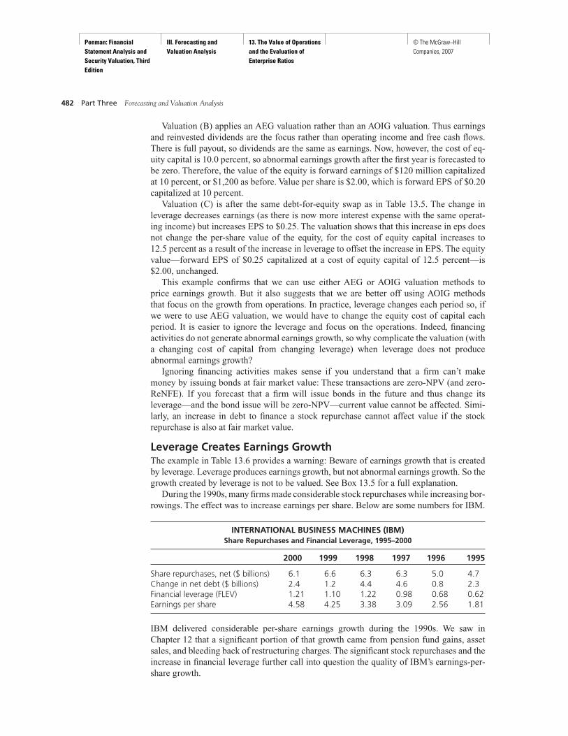
During the 1990s, many firms made considerable stock repurchases while increasing bor-rowings. The effect was to increase earnings per share. Below are some numbers for IBM.
INTERNATIONAL BUSINESS MACHINES (IBM)Share Repurchases and Financial Leverage, 1995–2000
2000 1999 1998 1997 1996 1995
Share repurchases, net ($ billions) 6.1 6.6 6.3 6.3 5.0 4.7Change in net debt ($ billions) 2.4 1.2 4.4 4.6 0.8 2.3Financial leverage (FLEV) 1.21 1.10 1.22 0.98 0.68 0.62Earnings per share 4.58 4.25 3.38 3.09 2.56 1.81
IBM delivered considerable per-share earnings growth during the 1990s. We saw inChapter 12 that a significant portion of that growth came from pension fund gains, assetsales, and bleeding back of restructuring charges. The significant stock repurchases and theincrease in financial leverage further call into question the quality of IBM’s earnings-per-share growth.
482 Part Three Forecasting and Valuation Analysis
Penman: Financial Statement Analysis and Security Valuation, Third Edition
III. Forecasting and Valuation Analysis
13. The Value of Operations and the Evaluation of Enterprise Ratios
© The McGraw−Hill Companies, 2007
483
(continued)
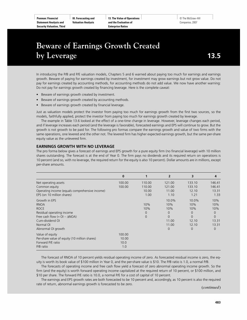
In introducing the P/B and P/E valuation models, Chapters 5 and 6 warned about paying too much for earnings and earningsgrowth. Beware of paying for earnings created by investment, for investment may grow earnings but not grow value. Do notpay for earnings created by accounting methods, for accounting methods do not add value. We now have another warning:Do not pay for earnings growth created by financing leverage. Here is the complete caveat:
• Beware of earnings growth created by investment.
• Beware of earnings growth created by accounting methods.
• Beware of earnings growth created by financial leverage.
Just as valuation models protect the investor from paying too much for earnings growth from the first two sources, so themodels, faithfully applied, protect the investor from paying too much for earnings growth created by leverage.
The example in Table 13.6 looked at the effect of a one-time change in leverage. However, leverage changes each period,and if leverage increases each period (and the leverage is favorable), forecasted earnings and EPS will continue to grow. But thegrowth is not growth to be paid for. The following pro formas compare the earnings growth and value of two firms with thesame operations, one levered and the other not. The levered firm has higher expected earnings growth, but the same per-shareequity value as the unlevered firm.
EARNINGS GROWTH WITH NO LEVERAGEThe pro forma below gives a forecast of earnings and EPS growth for a pure equity firm (no financial leverage) with 10 millionshares outstanding. The forecast is at the end of Year 0. The firm pays no dividends and its required return on operations is10 percent (and so, with no leverage, the required return for the equity is also 10 percent). Dollar amounts are in millions, exceptper-share amounts.
0 1 2 3 4
Net operating assets 100.00 110.00 121.00 133.10 146.41Common equity 100.00 110.00 121.00 133.10 146.41Operating income (equals comprehensive income) 10.00 11.00 12.10 13.31EPS (on 10 million shares) 1.00 1.10 1.21 1.33
Growth in EPS 10.0% 10.0% 10%RNOA 10% 10% 10% 10%ROCE 10% 10% 10% 10%Residual operating income 0 0 0 0Free cash flow (= OI − ∆NOA) 0 0 0 0Cum-dividend OI 11.00 12.10 13.31Normal OI 11.00 12.10 13.31Abnormal OI growth 0 0 0
Value of equity 100.00Per-share value of equity (10 million shares) 10.00Forward P/E ratio 10.0P/B ratio 1.0
The forecast of RNOA of 10 percent yields residual operating income of zero. As forecasted residual income is zero, the eq-uity is worth its book value of $100 million in Year 0, and the per-share value is $10. The P/B ratio is 1.0, a normal P/B.
The forecasts of operating income and free cash flow yield a forecast of zero abnormal operating income growth. So thefirm (and the equity) is worth forward operating income capitalized at the required return of 10 percent, or $100 million, and$10 per share. The forward P/E ratio is 10.0, a normal P/E for a cost of capital of 10 percent.
The earnings and EPS growth rates are both forecasted to be 10 percent and, accordingly, as 10 percent is also the requiredrate of return, abnormal earnings growth is forecasted to be zero.
Beware of Earnings Growth Created by Leverage 13.5
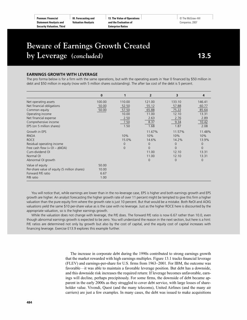
Penman: Financial Statement Analysis and Security Valuation, Third Edition
III. Forecasting and Valuation Analysis
13. The Value of Operations and the Evaluation of Enterprise Ratios
© The McGraw−Hill Companies, 2007
EARNINGS GROWTH WITH LEVERAGEThe pro forma below is for a firm with the same operations, but with the operating assets in Year 0 financed by $50 million indebt and $50 million in equity (now with 5 million shares outstanding). The after tax cost of the debt is 5 percent.
0 1 2 3 4
Net operating assets 100.00 110.00 121.00 133.10 146.41Net financial obligations 50.00 52.50 55.12 57.88 60.77Common equity 50.00 57.50 65.88 75.22 85.64Operating income 10.00 11.00 12.10 13.31Net financial expense 2.50 2.63 2.76 2.89Comprehensive income 7.50 8.37 9.34 10.42EPS (on 5 million shares) 1.50 1.68 1.87 2.08
Growth in EPS 11.67% 11.57% 11.48%RNOA 10% 10% 10% 10%ROCE 15.0% 14.6% 14.2% 13.9%Residual operating income 0 0 0 0Free cash flow (= OI − ∆NOA) 0 0 0 0Cum-dividend OI 11.00 12.10 13.31Normal OI 11.00 12.10 13.31Abnormal OI growth 0 0 0
Value of equity 50.00Per-share value of equity (5 million shares) 10.00Forward P/E ratio 6.67P/B ratio 1.00
You will notice that, while earnings are lower than in the no-leverage case, EPS is higher and both earnings growth and EPSgrowth are higher. An analyst forecasting the higher growth rate of over 11 percent might be tempted to give this firm a highervaluation than the pure equity firm where the growth rate is just 10 percent. But that would be a mistake. Both ReOI and AOIGvaluations yield the same $10 per-share value as is the case with no leverage. Just as the higher ROCE here is discounted by theappropriate valuation, so is the higher earnings growth.
While the valuation does not change with leverage, the P/E does. The forward P/E ratio is now 6.67 rather than 10.0, eventhough abnormal earnings growth is expected to be zero. You will understand the reason in the next section, but here is a hint:P/E ratios are determined not only by growth but also by the cost of capital, and the equity cost of capital increases withfinancing leverage. Exercise E13.9 explores this example further.
The increase in corporate debt during the 1990s contributed to strong earnings growththat the market rewarded with high earnings multiples. Figure 13.1 tracks financial leverage(FLEV) and earnings-per-share for U.S. firms from 1963–2001. For IBM, the outcome wasfavorable—it was able to maintain a favorable leverage position. But debt has a downside,and this downside risk increases the required return: If leverage becomes unfavorable, earn-ings will decline, perhaps precipitously. For some firms, the downside of debt became ap-parent in the early 2000s as they struggled to cover debt service, with large losses of share-holder value. Vivendi, Quest (and the many telecoms), United Airlines (and the many aircarriers) are just a few examples. In many cases, the debt was issued to make acquisitions
484
Beware of Earnings Growth Created by Leverage (concluded) 13.5

Penman: Financial Statement Analysis and Security Valuation, Third Edition
III. Forecasting and Valuation Analysis
13. The Value of Operations and the Evaluation of Enterprise Ratios
© The McGraw−Hill Companies, 2007
that also produced earnings growth. Analysts must be aware of earnings growth from ac-quisitions, but especially when the growth is financed with debt. A similar warning attachesto stock repurchases. See Box 13.6.
Debt and TaxesSome people argue that, because interest is tax-deductible if paid by a corporation but is notdeductible if paid by shareholders, there are tax savings to corporate borrowing. Share-holders can borrow on personal account to lever their equity, but they can also lever theirequity by borrowing within the firm. If they borrow within the firm, they add value becausethey get a tax deduction for the interest cost incurred.
The claim is controversial. First, interest can (in the U.S.) be deducted on shareholders’own tax returns to the extent that it is matched by investment income. Second, the interestthat is deductible by corporations is taxable in the hands of debtholders who receive the in-terest, and they will require a higher interest rate to compensate them for the taxes, miti-gating the tax advantage to the corporate debt. The spread between interest rates on tax-freedebt (like municipal debt) and corporate debt suggests this is so. Third, free cash flow musteither be used to reduce corporate net debt or to make distributions to shareholders: C − I =d + F. Both uses have tax effects. If cash flow is applied to reduce debt, shareholders losethe tax advantage of debt; if the firm wishes to maintain the debt, it must distribute cashflow to shareholders who are then taxed on the distributions. Either way, free cash flow istaxed, and shareholders cannot get the tax advantage of debt without incurring taxes at thepersonal level.
You can delve into these issues in a corporate finance text. Armed with the shareholders’personal tax rates and the corporate tax rate, you can revise the value calculations here byincorporating the present value of tax benefits if you are convinced that debt adds value.(But do not fall into the trap of thinking only about the tax benefit of debt without consid-ering taxes on distributions to shareholders.)
Box 13.7 considers another way that firms might generate value for shareholders fromdebt.
Chapter 13 The Value of Operations and the Evaluation of Enterprise Price-to-Book Ratios and Price-Earnings Ratios 485
FIGURE 13.1Median FinancialLeverage for U.S.Firms, 1963–2001Financial leverageis net financialobligations to commonequity (FLEV).
Source:Company: Standard & Poor’sData: Compustat® data
0.7
Fina
ncia
l Lev
erag
e (F
LE
V)
0.6
0.5
0.4
0.3
0.2
0.1
0
1963
1965
1967
1969
1971
1973
1975
1977
1979
1981
1983
1985
1987
1989
1991
1993
1995
1997
1999
2001

Penman: Financial Statement Analysis and Security Valuation, Third Edition
III. Forecasting and Valuation Analysis
13. The Value of Operations and the Evaluation of Enterprise Ratios
© The McGraw−Hill Companies, 2007
Why Do Firms Repurchase Stock? 13.6
Firms make stock repurchases for very good reasons: They area method of paying out cash to shareholders. If a firm has sig-nificant holdings of financial assets and no investment oppor-tunities for the cash, they should pay it out to shareholders,who may indeed have those opportunities. The shareholderscan be no worse off, for at the very least, they can invest thecash in the same interest-bearing financial assets as the firm.
However, stock repurchases must be evaluated with care.Selling financial assets at fair value and paying the proceedsout with a fair value repurchase of stock does not createvalue; nor does issuing debt at fair value to finance a repur-chase. But management may have reasons for stock repur-chases other than passing out idle cash:
1. In a 2003 management survey,* 76 percent of respon-dents said that increasing earnings per share was an im-portant factor in share repurchase decisions. Repurchasesindeed increase earnings per share, but growth in earningsper share from share repurchases does not create value. Ifmanagement’s bonuses are tied to earnings per share, onecan see how they might favor repurchases.
2. In the same survey, 68 percent of respondents said thatreversing the dilutive effects of employee stock options isalso important. But stock repurchases do not reverse dilu-tion. See the discussion in Box 8.7 in Chapter 8.
3. Share repurchases are sometimes made when a firm isflush with cash as a result of its success. That can coincidewith a high stock price. Buying back overpriced stock de-stroys value for shareholders, even though increasing earn-
ings per share. Indeed, if the stock price is EPS driven, man-agement may be tempted to buy back overpriced stock toperpetuate EPS growth. You see how a price bubble couldresult.
4. Alternatively, management can create value for sharehold-ers by actively timing the market: “Buy low” applies tofirms buying their own stock as well as to investors. Ac-cordingly, management should be aware of the intrinsicvalue of the shares when they engage in share purchases(or issues). The 2003 management survey found that 86.4percent of managers say they repurchase when they con-sider their stock a good value.
If management are repurchasing stock with shareholdersfunds, check their insider trading filings with the SEC: Aremanagement buying or selling? Be particularly vigilant whenyou estimate that the stock is overpriced in the market.
In 2004, Google Inc., the Internet search engine company,went public with an IPO price of just under $90 per share.Within a year, its stock price had soared to over $300 and itsforward P/E to 90. The firm then announced a share issue toraise a further $4 billion. With $3 million in financial assets,strong cash flow, and no obvious investment plans, commen-tators questioned why Google would raise additional cash.Could it have been that Google’s management considered thestock to be overpriced at a P/E of 90 and thus a good time tosell?* A. Brav, J. Graham, R. Campbell, and R. Michaely, “Payout Policy inthe 21st Century,” Unpublished paper, Duke University, 2004.
MARK-TO-MARKET ACCOUNTING: A TOOL FOR INCORPORATINGTHE COST OF STOCK OPTIONS IN VALUATION
The distinction between operating activities and financing activities shows us that there aretwo ways to proceed in valuation. We can forecast future earnings from an asset or liability(and add the present value of its expected residual earnings to its book value), or we canmark the asset or liability to market. Marking to market is attractive because it relieves usof the forecasting task. But marking to market can only be done if market values are reli-able measures of fair value. Market values of financial assets and liabilities typically mea-sure up to this criterion, so we do not have to forecast the income and expenses arising fromfinancing activities.
Chapter 8 explained that shareholders incur losses when employees exercise the stockoptions they have received as compensation. Yet GAAP accounting does not recognize thisloss. In that chapter we showed how losses from the exercise on stock options are incorpo-rated in comprehensive income. But that is not the end of the matter. While recognizing theeffect of option exercises on current income, it does not accommodate outstanding optionsthat might be exercised in the future, decreasing future comprehensive income. A valuationbased on forecasting GAAP operating income will overestimate the value of the firm,
486

Penman: Financial Statement Analysis and Security Valuation, Third Edition
III. Forecasting and Valuation Analysis
13. The Value of Operations and the Evaluation of Enterprise Ratios
© The McGraw−Hill Companies, 2007
leaving the investor with the risk of paying too much for a stock. The analyst must make ad-justments. One might think the solution would involve reducing forecasts of GAAP earn-ings by forecasts of future losses from the exercise of options. Indeed, this is a solution. Butforecasting those losses is not an easy task: As the loss is the difference between the mar-ket price and the exercise price at the exercise date, one would have to anticipate not onlyexercise dates but the market price of the stock at those dates.
Mark-to-market accounting—the alternative to forecasting—provides a solution. Fairvalues of outstanding options can be estimated, with reasonable precision, using optionpricing methods. Nike’s stock option footnote, required by FASB Statement No. 123, givesdetails of outstanding options at the end of 2004:
Options Outstanding Options Exercisable
Weighted- Weighted- Weighted-Number of Average Average Number of Average
Options Exercise Contractual Options ExerciseExercise Price Outstanding Price Life Remaining Exercisable Price
(In thousands) (Years) (In thousands)$14.94–$27.69 1,771 $26.87 5.20 1,754 $26.8628.13–42.36 3,223 42.26 7.05 1,216 42.1442.50–48.44 1,870 47.57 3.93 1,828 47.6248.65–48.98 4,332 48.98 8.12 762 48.9849.01–52.24 5,008 52.19 9.02 135 50.6252.44–74.88 2,605 55.90 4.80 2,483 55.71
With Nike’s stock trading at $75 at the time, the weighted-average exercise prices hereindicate that many of the 18,809 thousand total outstanding options are in the money. The
Generating Value for Shareholders from Debt 13.7
Typically it is argued that firms cannot create value by issuingdebt: If the debt is issued at fair market value, the transactionis a zero-net present value transaction—or, equivalently, azero-residual net financial expense transaction. Banks andother financial institutions make money from the spread be-tween lending rates and borrowing rates and so create valuefrom transacting in debt. And bond traders who discover mis-pricing of bonds also create value from transacting in debt.But for the firm that uses debt for financing, debt transactionsare deemed not to create value.
There are exceptions, however.
1. Consider the following scenario. A firm with a particularrisk profile that is given an AAB bond rating issues debtwith a yield to maturity of 8 percent. Subsequently it en-gages in more risky business and the bonds accordingly aredowngraded to a BBB rating. The price of the bonds dropsto yield an 11 percent return commensurate with thefirm’s new risk level. The firm then redeems the bonds andbooks a gain.
Firms can transfer value from bondholders to share-holders in this way. There is a message for bondholders:Beware and write bond agreements that give protectionfrom this scenario. There is also a message for sharehold-ers: Bondholders can be exploited in this way. There is alsoa message for the valuation analyst: Firms can create valuefor shareholders in this scenario. Applying residual earn-ings techniques will incorporate this value. If the scenariois anticipated, the analyst forecasts a realized gain fromthe redemption of bonds and, accordingly, a negativeresidual net financial expense (that is, residual incomefrom bonds).
2. Just as management might time a share issue or repur-chase, they can time debt issues and repurchases. If man-agers think that the firm’s bonds are overpriced—becausethe market underestimates the default probability—theymight issue bonds to take advantage of the perceived mis-pricing. Correspondingly an underpricing of bonds maypromote a repurchase of the debt.
487
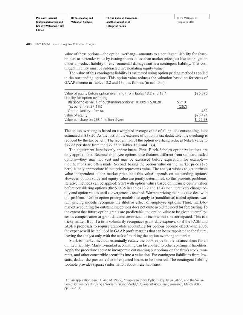
Penman: Financial Statement Analysis and Security Valuation, Third Edition
III. Forecasting and Valuation Analysis
13. The Value of Operations and the Evaluation of Enterprise Ratios
© The McGraw−Hill Companies, 2007
value of these options—the option overhang—amounts to a contingent liability for share-holders to surrender value by issuing shares at less than market price, just like an obligationunder a product liability or environmental damage suit is a contingent liability. That con-tingent liability must be subtracted in calculating equity value.
The value of this contingent liability is estimated using option pricing methods appliedto the outstanding options. This option value reduces the valuation based on forecasts ofGAAP income in Tables 13.2 and 13.4, as follows (in millions):
Value of equity before option overhang (from Tables 13.2 and 13.4) $20,876Liability for option overhang:
Black-Scholes value of outstanding options: 18.809 × $38.20 $ 719Tax benefit (at 37.1%) (267)Option liability, after tax 452
Value of equity $20,424Value per share on 263.1 million shares $ 77.63
The option overhang is based on a weighted-average value of all options outstanding, hereestimated at $38.20. As the loss on the exercise of option is tax deductible, the overhang isreduced by the tax benefit. The recognition of the option overhang reduces Nike’s value to$77.63 per share from the $79.35 in Tables 13.2 and 13.4.
The adjustment here is only approximate. First, Black-Scholes option valuations areonly approximate. Because employee options have features different from standard tradedoptions—they may not vest and may be exercised before expiration, for example—modifications are often made. Second, basing the option value on the market price ($75here) is only appropriate if that price represents value. The analyst wishes to get intrinsicvalue independent of the market price, and this value depends on outstanding options.However, option value and equity value are jointly determined, so this presents problems.Iterative methods can be applied: Start with option values based on intrinsic equity valuesbefore considering options (the $79.35 in Tables 13.2 and 13.4) then iteratively change eq-uity and option values until convergence is reached. Warrant pricing methods also deal withthis problem.1 Unlike option pricing models that apply to (nondilutive) traded options, war-rant pricing models recognize the dilutive effect of employee options. Third, mark-to-market accounting for outstanding options does not quite avoid the need for forecasting. Tothe extent that future option grants are predictable, the option value to be given to employ-ees as compensation at grant date and amortized to income must be anticipated. This is atricky matter. But, if a firm voluntarily recognizes grant-date expense, or if the FASB andIASB’s proposals to require grant-date accounting for options become effective in 2006,the expense will be included in GAAP profit margins that can be extrapolated to the future,leaving the analyst only with the task of marking the option overhang to market.
Mark-to-market methods essentially restate the book value on the balance sheet for anomitted liability. Mark-to-market accounting can be applied to other contingent liabilities.Apply the procedure above to incorporate outstanding put options on the firm’s stock, war-rants, and other convertible securities into a valuation. For contingent liabilities from law-suits, deduct the present value of expected losses to be incurred. The contingent liabilityfootnote provides (sparse) information about these liabilities.
488 Part Three Forecasting and Valuation Analysis
1 For an application, see F. Li and M. Wong, “Employee Stock Options, Equity Valuation, and the Valua-tion of Option Grants Using a Warrant-Pricing Model,” Journal of Accounting Research, March 2005,pp. 97–131.
Penman: Financial Statement Analysis and Security Valuation, Third Edition
III. Forecasting and Valuation Analysis
13. The Value of Operations and the Evaluation of Enterprise Ratios
© The McGraw−Hill Companies, 2007
ENTERPRISE MULTIPLES
In the example of leverage effects in Table 13.5 you will have noticed that the P/B ratioincreased with the increase in leverage, from 1.2 to 1.33. You also will have noticed that theP/E ratio decreased with the increase in leverage in Table 13.6, from 10 to 8. Yet, in bothcases, the value of the equity did not change. This suggests that we might be better servedto think of P/B and P/E ratios without the effect of leverage.
Enterprise Price-to-Book RatiosThe value of equity is the value of the operations minus the value of the net financial oblig-ations. So the intrinsic price-to-book (P/B) ratio can be expressed as
If the net financial obligations are measured at market value, they do not contribute to thepremium over book value; the difference between price and book value is due to net oper-ating assets not being measured at market value. Yet the expression here tells us that the P/Bratio will vary as the amount of net financial obligations changes relative to the operatingassets. That is, the ratio is sensitive to leverage. So differences in firms’ P/B ratios can de-rive from their financing even though price equals book value for financial items.
To avoid this confusion we should focus on the value of the operations relative to theirbook value. The ratio of the value of the net operating assets to their book value is theenterprise P/B ratio or the unlevered P/B ratio:
The value of the net operating assets is, of course, the value of the equity plus the netfinancial obligations. So, to calculate a market (traded) enterprise P/B, just add the netfinancial obligations to the market value of the equity.
The standard price-to-book ratio for the equity is referred to as the levered P/B ratio.The two P/B ratios reconcile as follows:
Levered P/B ratio = Enterprise P/B ratio (13.10)+ [Financial leverage × (Enterprise P/B ratio – 1)]
where FLEV is book financial leverage (NFO/CSE), as before. The difference between thetwo P/B ratios increases with leverage and the distance that the unlevered P/B is from thenormal of 1.0. For an unlevered P/B of 1.0, the levered P/B is also 1.0 regardless of lever-age. Figure 13.2A shows how the levered P/B ratio changes with leverage for six differentlevels of the unlevered P/B ratio. The conversion chart in Figure 13.2B charts unleveredP/B ratios corresponding to levered P/B ratios for different leverage levels.
The levered P/B ratio is the one that is commonly referred to. But it is the enterprise P/Bon which we should focus. Reebok’s levered P/B before its large stock repurchase andchange in leverage (in Box 13.4) was 3.3, but immediately after it was 6.3. This change
V V VE0
0
0
0 01
CSE NOAFLEV
NOA
NOA0NOA
= + −⎛
⎝⎜⎞
⎠⎟
Enterprise P/B ratioValue of net operating assets
Net operating assets
NOA
NOA
0
=
= V0
V V VE0
0
0 0
CSE NOA – NFO
NOA NFO
= −
Chapter 13 The Value of Operations and the Evaluation of Enterprise Price-to-Book Ratios and Price-Earnings Ratios 489

Penman: Financial Statement Analysis and Security Valuation, Third Edition
III. Forecasting and Valuation Analysis
13. The Value of Operations and the Evaluation of Enterprise Ratios
© The McGraw−Hill Companies, 2007
does not reflect a change in the expected profitability of operations or a change in the pre-mium one would have paid for the operations. It’s a leverage-induced change: Reebok’senterprise P/B remained the same at 3.0. And the stock price was unchanged at about $36;this repurchase and financing transaction had no effect on shareholders’ per-share value,and this is also indicated by no change in the enterprise P/B ratio.
Figure 13.3 plots the median levered and unlevered price-to-book ratios for U.S. firmsfrom 1963 to 2003. When unlevered P/B ratios were around 1.0 in the mid-1970s, so werethe levered ratios. But when unlevered P/B ratios were above 1.0, the levered P/B ratioswere higher than the unlevered ratios, the more so the higher the unlevered P/B.
Enterprise Price-Earnings RatiosThe P/E ratio commonly referred to prices earnings after net interest expense, so it is alevered P/E. A levered P/E ratio anticipates earnings growth. However, earnings growth isaffected by leverage, and anticipated growth from leverage is not growth to be valued be-cause it creates no abnormal earnings growth. So it makes sense to think of a P/E ratio interms of growth in earnings from operations. The enterprise P/E ratio or unlevered P/Eratio prices the operating income on the basis of expected growth in operating income.
490 Part Three Forecasting and Valuation Analysis
FIGURE 13.2ALevered P/B Ratiosand LeverageThe figure shows howthe levered P/B ratio(VE/CSE) changeswith financial leveragefor different levels ofunlevered P/B(VNOA/NOA).
7.0
6.0
5.0
4.0
3.0
2.0
1.0
0.0
–1.0
0.3 0.5 0.8 1.0 1.3 1.5 1.8 2.0 2.3
Lev
ered
P/B
(V
E/C
SE)
VE
CSEVNOA
NOAVNOA
NOA= + FLEV –1
Leverage (NFO/CSE)
0.0
VNOA/NOA = 3
VNOA/NOA = 2.5
VNOA/NOA = 2
VNOA/NOA = 1.5
VNOA/NOA = 1
VNOA/NOA = 0.5
Levered P/B versus Financial Leverage
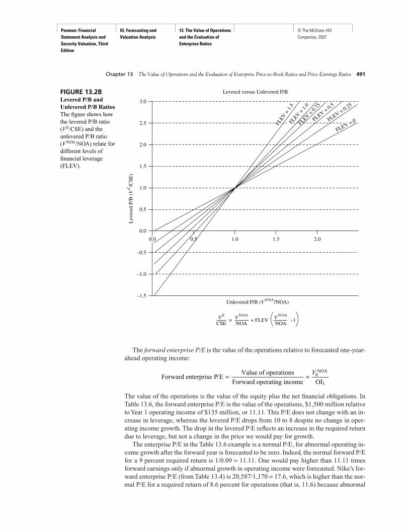
Penman: Financial Statement Analysis and Security Valuation, Third Edition
III. Forecasting and Valuation Analysis
13. The Value of Operations and the Evaluation of Enterprise Ratios
© The McGraw−Hill Companies, 2007
The forward enterprise P/E is the value of the operations relative to forecasted one-year-ahead operating income:
The value of the operations is the value of the equity plus the net financial obligations. InTable 13.6, the forward enterprise P/E is the value of the operations, $1,500 million relativeto Year 1 operating income of $135 million, or 11.11. This P/E does not change with an in-crease in leverage, whereas the levered P/E drops from 10 to 8 despite no change in oper-ating income growth. The drop in the levered P/E reflects an increase in the required returndue to leverage, but not a change in the price we would pay for growth.
The enterprise P/E in the Table 13.6 example is a normal P/E, for abnormal operating in-come growth after the forward year is forecasted to be zero. Indeed, the normal forward P/Efor a 9 percent required return is 1/0.09 = 11.11. One would pay higher than 11.11 timesforward earnings only if abnormal growth in operating income were forecasted. Nike’s for-ward enterprise P/E (from Table 13.4) is 20,587/1,170 = 17.6, which is higher than the nor-mal P/E for a required return of 8.6 percent for operations (that is, 11.6) because abnormal
Forward enterprise P/EValue of operations
Forward operating income OI
NOA
= = V0
1
Chapter 13 The Value of Operations and the Evaluation of Enterprise Price-to-Book Ratios and Price-Earnings Ratios 491
3.0
2.5
2.0
1.5
1.0
0.5
0.0
–0.5
–1.0
–1.5
0.5 1.0 1.5 2.0
Lev
ered
P/B
(V
E/C
SE)
VE
CSEVNOA
NOAVNOA
NOA= + FLEV –1
Unlevered P/B (VNOA/NOA)
0.0
FLEV = 0.25
FLEV = 0.5
FLEV
= 1
.5
FLEV = 0FLEV = 0.
75
FLEV = 1.
0
Levered versus Unlevered P/BFIGURE 13.2BLevered P/B andUnlevered P/B RatiosThe figure shows howthe levered P/B ratio(VE/CSE) and theunlevered P/B ratio(VNOA/NOA) relate fordifferent levels offinancial leverage(FLEV).
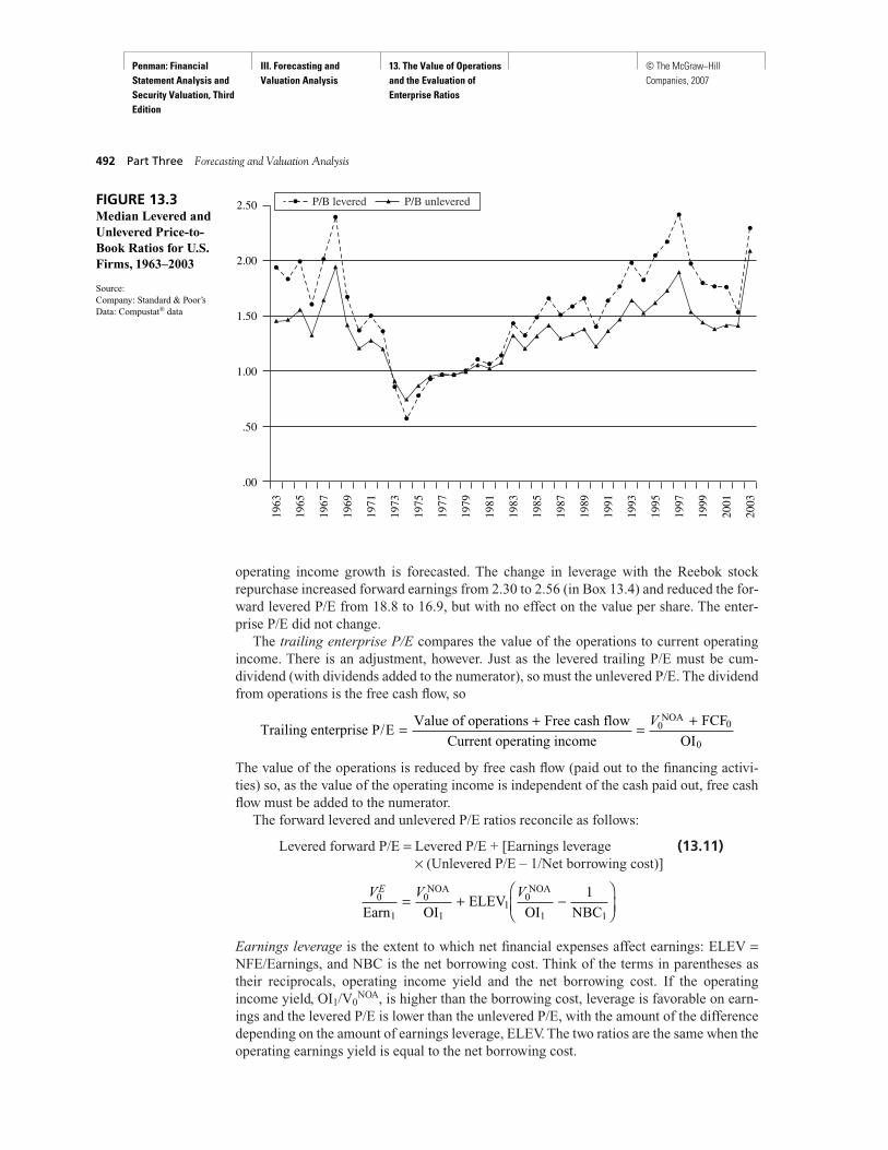
Penman: Financial Statement Analysis and Security Valuation, Third Edition
III. Forecasting and Valuation Analysis
13. The Value of Operations and the Evaluation of Enterprise Ratios
© The McGraw−Hill Companies, 2007
operating income growth is forecasted. The change in leverage with the Reebok stockrepurchase increased forward earnings from 2.30 to 2.56 (in Box 13.4) and reduced the for-ward levered P/E from 18.8 to 16.9, but with no effect on the value per share. The enter-prise P/E did not change.
The trailing enterprise P/E compares the value of the operations to current operatingincome. There is an adjustment, however. Just as the levered trailing P/E must be cum-dividend (with dividends added to the numerator), so must the unlevered P/E. The dividendfrom operations is the free cash flow, so
The value of the operations is reduced by free cash flow (paid out to the financing activi-ties) so, as the value of the operating income is independent of the cash paid out, free cashflow must be added to the numerator.
The forward levered and unlevered P/E ratios reconcile as follows:
Levered forward P/E = Levered P/E + [Earnings leverage (13.11)× (Unlevered P/E – 1/Net borrowing cost)]
Earnings leverage is the extent to which net financial expenses affect earnings: ELEV =NFE/Earnings, and NBC is the net borrowing cost. Think of the terms in parentheses astheir reciprocals, operating income yield and the net borrowing cost. If the operatingincome yield, OI1/V0
NOA, is higher than the borrowing cost, leverage is favorable on earn-ings and the levered P/E is lower than the unlevered P/E, with the amount of the differencedepending on the amount of earnings leverage, ELEV. The two ratios are the same when theoperating earnings yield is equal to the net borrowing cost.
V V VE0
1
0
1 1 1
1
Earn OIELEV
OI NBC
NOA
10NOA
= + −⎛
⎝⎜⎞
⎠⎟
Trailing enterprise P/EValue of operations Free cash flow
Current operating income
FCF
OI
NOA
= + = +V0 0
0
492 Part Three Forecasting and Valuation Analysis
2.00
2.50
1.50
1.00
.50
.00
1963
1965
1967
1969
1971
1973
1975
1977
1979
1981
1983
1985
1987
1989
1991
1993
1995
1997
1999
2001
2003
P/B levered P/B unleveredFIGURE 13.3Median Levered andUnlevered Price-to-Book Ratios for U.S.Firms, 1963–2003
Source:Company: Standard & Poor’sData: Compustat® data
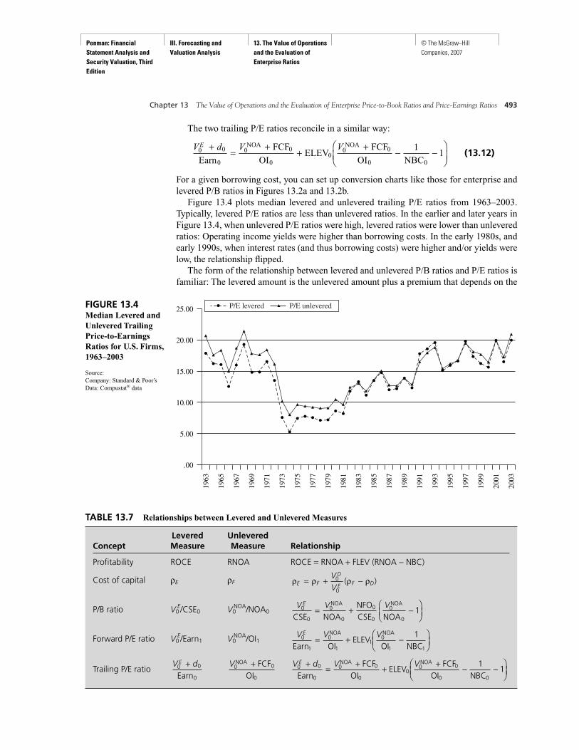
Penman: Financial Statement Analysis and Security Valuation, Third Edition
III. Forecasting and Valuation Analysis
13. The Value of Operations and the Evaluation of Enterprise Ratios
© The McGraw−Hill Companies, 2007
Chapter 13 The Value of Operations and the Evaluation of Enterprise Price-to-Book Ratios and Price-Earnings Ratios 493
20.00
25.00
15.00
10.00
5.00
.00
1963
1965
1967
1969
1971
1973
1975
1977
1979
1981
1983
1985
1987
1989
1991
1993
1995
1997
1999
2001
2003
P/E levered P/E unleveredFIGURE 13.4Median Levered andUnlevered TrailingPrice-to-EarningsRatios for U.S. Firms,1963–2003
Source:Company: Standard & Poor’sData: Compustat® data
The two trailing P/E ratios reconcile in a similar way:
(13.12)
For a given borrowing cost, you can set up conversion charts like those for enterprise andlevered P/B ratios in Figures 13.2a and 13.2b.
Figure 13.4 plots median levered and unlevered trailing P/E ratios from 1963–2003.Typically, levered P/E ratios are less than unlevered ratios. In the earlier and later years inFigure 13.4, when unlevered P/E ratios were high, levered ratios were lower than unleveredratios: Operating income yields were higher than borrowing costs. In the early 1980s, andearly 1990s, when interest rates (and thus borrowing costs) were higher and/or yields werelow, the relationship flipped.
The form of the relationship between levered and unlevered P/B ratios and P/E ratios isfamiliar: The levered amount is the unlevered amount plus a premium that depends on the
V d V VE0 0
0
0 0
0
0
0 0
11
+ = + + + − −⎛
⎝⎜⎞
⎠⎟Earn
FCF
OIELEV
FCF
OI NBC
NOA
00NOA
TABLE 13.7 Relationships between Levered and Unlevered Measures
Levered UnleveredConcept Measure Measure Relationship
Profitability ROCE RNOA ROCE = RNOA + FLEV (RNOA − NBC)
Cost of capital ρE ρF
P/B ratio V0E/CSE0 V0
NOA/NOA0
Forward P/E ratio V0E/Earn1 V0
NOA/OI1
Trailing P/E ratioV d V VE
0 0
0
0 0
0
0
0 0
11
+ = + + + − −⎛⎝⎜
⎞⎠⎟Earn
FCFOI
ELEVFCF
OI NBC
NOA
00NOAV0 0
0
NOA FCFOI
+V dE0 0
0
+Earn
V V VE0
1
0
11
0
1 1
1Earn OI
ELEVOI NBC
NOA NOA= + −
⎛⎝⎜
⎞⎠⎟
V V VE0
0
0
0
0 0 1CSE NOA
NFOCSE NOA
NOA
0
NOA
0= + −
⎛⎝⎜
⎞⎠⎟
ρ ρ ρ ρE F
D
E F DVV
= + −0
0
( )
Penman: Financial Statement Analysis and Security Valuation, Third Edition
III. Forecasting and Valuation Analysis
13. The Value of Operations and the Evaluation of Enterprise Ratios
© The McGraw−Hill Companies, 2007
494 Part Three Forecasting and Valuation Analysis
The Web Connection
Find the following on the Web page for this chapter:
• Further explanation of residual operating incomemethods.
• Further explanation of abnormal operating incomegrowth methods.
• A further demonstration of the equivalence of residualearnings valuation and residual operating income valu-ation (and the cost of capital adjustments required).
• Demonstrations of how leverage affects ROCE, earn-ings growth, and valuations.
• More coverage of levered and unlevered P/B and P/Eratios.
• Further examples of the option overhang.
• Demonstration of how residual earnings valuationmethods can be applied to the impairment of goodwill.
leverage and a spread. We saw this in the relationship between levered and unleveredaccounting returns and required returns. Table 13.7 summarizes the leverage effects wehave discussed in this chapter.
Summary To the extent that accountants get the balance sheet correct, the analyst does not have tomake a valuation. If, in the extreme, the balance sheet were perfect—giving the value of theequity—the analyst would have nothing to do; the accountant would have done the valua-tion. Balance sheets are typically not perfect, so the analyst has to forecast to get the miss-ing value. But to the extent that the balance sheet gives the value, the analyst can avoidforecasting.
This chapter has introduced valuation approaches that recognize the balance sheet val-ues of net financial items as approximating their market values, but recognize that balancesheet amounts for net operating assets are typically not their values. Accordingly, valuationis based on forecasting residual income or abnormal earnings growth from operations. Thevaluation gives the value of the operations, and the value of the equity is then the value ofthe operations less the balance sheet value of the net debt (or the fair value of the net debtin the fair-value footnote).
If the net debt on the balance sheet is close to its fair value, the appropriate way of think-ing of a book value multiple is in terms of the unlevered or enterprise price-to-book ratio,that is, the pricing of the net operating assets rather than the equity. The chapter has laid outthe calculation of the enterprise price-to-book ratio and has shown how it relates, throughleverage, to the levered price-to-book ratio.
This chapter also focused on enterprise price-earnings ratios. It recognized that standardP/E ratios—levered P/E ratios—are based on prospective earnings growth that incorporatesgrowth that is created by leverage. Yet, growth from leverage is not valued. Levered P/E ra-tios change with leverage, even if leverage has no effect on equity value. The analyst there-fore prices growth from operations with an enterprise or unlevered P/E ratio.
We always want to carry out valuations efficiently. The residual operating income valua-tion approach and the abnormal operating income growth approach both reduce the fore-casting task on which we will embark in the next two chapters. Only the operating compo-nents of comprehensive income and the net operating asset component on the balance sheetneed to be forecasted. Further, in converting forecasts to a valuation using a required return,one can ignore changes in required returns that are due to changes in financial leverage.

Penman: Financial Statement Analysis and Security Valuation, Third Edition
III. Forecasting and Valuation Analysis
13. The Value of Operations and the Evaluation of Enterprise Ratios
© The McGraw−Hill Companies, 2007
Chapter 13 The Value of Operations and the Evaluation of Enterprise Price-to-Book Ratios and Price-Earnings Ratios 495
book leverage is the book value of netfinancial obligations relative to the book value of common shareholders’equity. 475
effective cost of debt is the after-tax costof borrowing. 473
enterprise value is the value of theoperations. 466
financing risk is the risk shareholders haveof losing value in borrowing and lendingactivities. 475
levered price-to-book ratio is theprice multiple of common equity.Compare with unlevered price-to-book ratio. 489
levered price-earnings ratio is the pricemultiple that prices (net) earnings.Compare with unlevered price-earningsratio. 490
market leverage is financial leveragemeasured by the ratio of the value of netfinancial obligations to the value ofcommon equity. 475
operating risk is the risk shareholders andbondholders have of losing value inoperations. 475
pure equity firm is a firm with no netdebt. 475
unlevered price-to-book ratio orenterprise price-to-book ratio is the pricemultiple of net operating assets. Comparewith levered price-to-book ratio. 489
unlevered price-earnings ratio orenterprise price-earnings ratio is theprice multiple that prices operatingincome. Compare with levered price-earnings ratio. 490
Key Concepts
The Analyst’s Toolkit
Residual operating incomevaluation modelequation 13.4 466
Abnormal operating incomegrowth modelequation 13.6 471
Weighted-average cost ofcapital (WACC)(equation 13.7) 473
Effective cost of debt 473Equity cost of capital
(equation 13.8) 475Valuation and leverage 475Valuation and stock
repurchases 479Valuation and stock options 486Levered and unlevered
price-to-book (P/B) ratios 489Levered and unlevered price-
earnings (P/E) ratios 490
Abnormal operating incomegrowth (AOIG) 470
After-tax cost of debt 473Earnings leverage (ELEV) 492Levered P/B ratio 489Market leverage 475Residual net financial expense
(ReNFE) 465Residual operating income
(ReOI) 465Unlevered P/B ratio 489Unlevered P/E ratio 490Weighted-average cost
of capital (WACC) 473
AOIG abnormal operatingincome growth
CAPM capital asset pricing modelCSE common shareholders’
equityCV continuing valueELEV earnings leverageFA financial assetsFCF free cash flowFLEV financial leverageNBC net borrowing costNFE net financial expenseNFO net financial obligationsNOA net operating assetsOI operating incomeP/B price-to-book ratioRE residual earningsReNFE residual net financial
expenseReOI residual operating incomeROCE return on common equityRNOA return on net operating
assetsWACC weighted-average cost
of capital
Analysis Tools Page Key Measures Page Acronyms to Remember
Penman: Financial Statement Analysis and Security Valuation, Third Edition
III. Forecasting and Valuation Analysis
13. The Value of Operations and the Evaluation of Enterprise Ratios
© The McGraw−Hill Companies, 2007
496 Part Three Forecasting and Valuation Analysis
A Continuing Case: Kimberly-Clark Corporation
A Self-Study ExerciseIn the next chapter you will begin to develop a valuation of KMB’s shares based on theanalysis work you have done to this point. In preparation, expand your analysis of two yearsof income to a full six years. The income statements for the three years 2002–2004 are inthe continuing case for Chapter 2, and you have thoroughly analyzed those for 2003–2004in Chapters 9–12. Below are the income statements for 1999–2001, along with some sup-plemental information on the firm’s net pension expense and the operating cash flowsection of the cash flow statement for those years. Also given is a summary of the firm’s netoperating assets and net financial obligations for 1998–2001.
Your task is to track Kimberly-Clark’s residual operating income over the years1999–2004. Also calculate abnormal operating income growth over the years. This historywill give you some insight into the likely path in the future. To do this, you will have toidentify after-tax operating income for all years. You will also have to estimate the cost ofcapital for operations.
THE COST OF CAPITAL FOR OPERATIONSFollow the procedures in Box 13.2. Strictly the cost of capital should be reestimated eachyear, but this is a very stable firm, so make the calculation for 2004 and apply it to all years.Calculate the market value of the equity on the basis of the per-share stock price of $64.81in early 2005 (see the Continuing Case for Chapter 1). You calculated the equity cost ofcapital, based on a beta of 0.88, in the Continuing Case for Chapter 3. The firm’s debt foot-note indicates a weighted-average borrowing rate of 5.77 percent (before tax). Be skepticalof these calculations. See Box 13.3.
TRACK THE DRIVERS OF RESIDUALOPERATING INCOMEHow much of the change in residual operating income over the years is due to profitability(RNOA) and how much to growth in net operating assets? Examine the effect of sales growth.How much of operating income growth comes from core operations? Compare the growth incore operating income with the growth in earnings per share. Why are they different?
THE 2005 STOCK REPURCHASEThe $1.6 billion stock repurchase in 2004 was a significant event. What effect will this haveon future operating profitability, return on common equity, and earnings per share growth?What effect would the repurchase have on the value per share?
OPTION OVERHANGThe stock option footnote indicates that there are 31.720 million employee stock optionsoutstanding at the end of 2004 with a weighted-average exercise price of $55.57. Theweighted-average value of these options is estimated at $16.25. Calculate the after-taxoption overhang.

Penman: Financial Statement Analysis and Security Valuation, Third Edition
III. Forecasting and Valuation Analysis
13. The Value of Operations and the Evaluation of Enterprise Ratios
© The McGraw−Hill Companies, 2007
ENTERPRISE P/B AND P/E RATIOSCalculate the levered and enterprise price-to-book ratios in early 2005 when the stock pricewas $64.81. Also calculate the levered and enterprise trailing P/E ratios. (KMB’s 2004 div-idend was $1.60 per share.) Show that the levered and unlevered multiples reconcile ac-cording to standard formulas.
Consolidated Income Statements
Year Ended December 31
(Millions of dollars, except per share amounts) 2001 2000 1999
Net sales $14,524.4 $13,982.0 $13,006.8Cost of products sold 8,615.5 8,228.5 7,681.6
Gross profit 5,908.9 5,753.5 5,325.2Advertising, promotion and selling expenses 2,334.4 2,122.7 2,097.8Research expense 295.3 277.4 249.8General expense 767.9 742.1 707.4Goodwill amortization 89.4 81.7 41.8Other (income) expense, net 83.7 (104.2) (207.0)
Operating profit 2,338.2 2,633.8 2,435.4Interest income 17.8 24.0 29.4Interest expense (191.6) (221.8) (213.1)
Income before income taxes 2,164.4 2,436.0 2,251.7Provision for income taxes 645.7 758.5 730.2
Income before equity interests 1,518.7 1,677.5 1,521.5Share of net income of equity companies 154.4 186.4 189.6Minority owners’ share of subsidiaries’
net income (63.2) (63.3) (43.0)Net income $ 1,609.9 $ 1,800.6 $ 1,668.1Net income per shareBasic $ 3.04 $ 3.34 $ 3.11Diluted $ 3.02 $ 3.31 $ 3.09
Consolidated Cash Flow Statement (Cash from Operations Section)
(Millions of dollars) 2001 2000 1999
OperationsNet income $1,609.9 $1,800.6 $1,668.1Depreciation 650.2 591.7 586.2Goodwill amortization 89.4 81.7 41.8Deferred income tax provision 39.7 84.1 126.2Net losses (gains) on asset dispositions 102.0 19.3 (143.9)Equity companies’ earnings in excess of
dividends paid (39.1) (67.0) (78.7)Minority owners’ share of subsidiaries’
net income 63.2 63.3 43.0Increase in operating working capital (232.6) (338.3) (61.5)Postretirement benefits (54.7) (121.9) (43.1)Other 25.8 19.7 1.8
Cash provided by operations 2,253.8 2,133.2 2,139.9
Chapter 13 The Value of Operations and the Evaluation of Enterprise Price-to-Book Ratios and Price-Earnings Ratios 497
(continued)
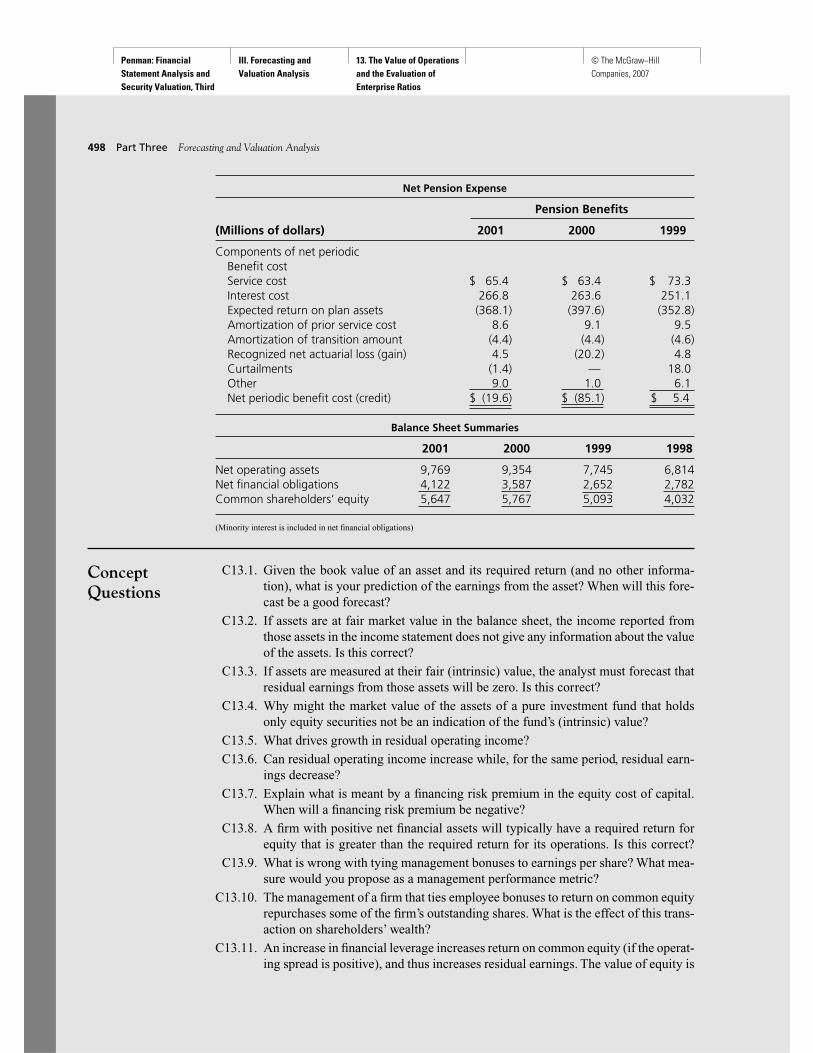
Penman: Financial Statement Analysis and Security Valuation, Third Edition
III. Forecasting and Valuation Analysis
13. The Value of Operations and the Evaluation of Enterprise Ratios
© The McGraw−Hill Companies, 2007
Net Pension Expense
Pension Benefits
(Millions of dollars) 2001 2000 1999
Components of net periodicBenefit costService cost $ 65.4 $ 63.4 $ 73.3Interest cost 266.8 263.6 251.1Expected return on plan assets (368.1) (397.6) (352.8)Amortization of prior service cost 8.6 9.1 9.5Amortization of transition amount (4.4) (4.4) (4.6)Recognized net actuarial loss (gain) 4.5 (20.2) 4.8Curtailments (1.4) — 18.0Other 9.0 1.0 6.1Net periodic benefit cost (credit) $ (19.6) $ (85.1) $ 5.4
Balance Sheet Summaries
2001 2000 1999 1998
Net operating assets 9,769 9,354 7,745 6,814Net financial obligations 4,122 3,587 2,652 2,782Common shareholders’ equity 5,647 5,767 5,093 4,032
(Minority interest is included in net financial obligations)
498 Part Three Forecasting and Valuation Analysis
ConceptQuestions
C13.1. Given the book value of an asset and its required return (and no other informa-tion), what is your prediction of the earnings from the asset? When will this fore-cast be a good forecast?
C13.2. If assets are at fair market value in the balance sheet, the income reported fromthose assets in the income statement does not give any information about the valueof the assets. Is this correct?
C13.3. If assets are measured at their fair (intrinsic) value, the analyst must forecast thatresidual earnings from those assets will be zero. Is this correct?
C13.4. Why might the market value of the assets of a pure investment fund that holdsonly equity securities not be an indication of the fund’s (intrinsic) value?
C13.5. What drives growth in residual operating income?
C13.6. Can residual operating income increase while, for the same period, residual earn-ings decrease?
C13.7. Explain what is meant by a financing risk premium in the equity cost of capital.When will a financing risk premium be negative?
C13.8. A firm with positive net financial assets will typically have a required return forequity that is greater than the required return for its operations. Is this correct?
C13.9. What is wrong with tying management bonuses to earnings per share? What mea-sure would you propose as a management performance metric?
C13.10. The management of a firm that ties employee bonuses to return on common equityrepurchases some of the firm’s outstanding shares. What is the effect of this trans-action on shareholders’ wealth?
C13.11. An increase in financial leverage increases return on common equity (if the operat-ing spread is positive), and thus increases residual earnings. The value of equity is
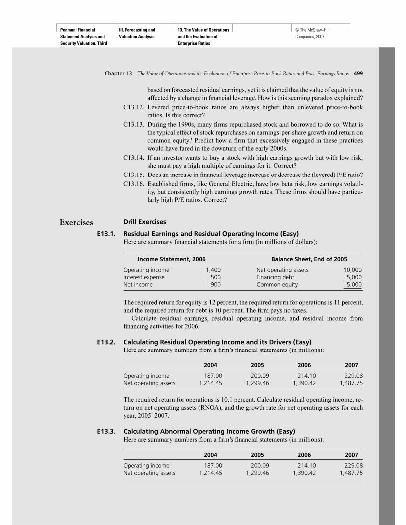
Penman: Financial Statement Analysis and Security Valuation, Third Edition
III. Forecasting and Valuation Analysis
13. The Value of Operations and the Evaluation of Enterprise Ratios
© The McGraw−Hill Companies, 2007
Chapter 13 The Value of Operations and the Evaluation of Enterprise Price-to-Book Ratios and Price-Earnings Ratios 499
based on forecasted residual earnings, yet it is claimed that the value of equity is notaffected by a change in financial leverage. How is this seeming paradox explained?
C13.12. Levered price-to-book ratios are always higher than unlevered price-to-bookratios. Is this correct?
C13.13. During the 1990s, many firms repurchased stock and borrowed to do so. What isthe typical effect of stock repurchases on earnings-per-share growth and return oncommon equity? Predict how a firm that excessively engaged in these practiceswould have fared in the downturn of the early 2000s.
C13.14. If an investor wants to buy a stock with high earnings growth but with low risk,she must pay a high multiple of earnings for it. Correct?
C13.15. Does an increase in financial leverage increase or decrease the (levered) P/E ratio?
C13.16. Established firms, like General Electric, have low beta risk, low earnings volatil-ity, but consistently high earnings growth rates. These firms should have particu-larly high P/E ratios. Correct?
Exercises Drill Exercises
E13.1. Residual Earnings and Residual Operating Income (Easy)Here are summary financial statements for a firm (in millions of dollars):
Income Statement, 2006 Balance Sheet, End of 2005
Operating income 1,400 Net operating assets 10,000Interest expense 500 Financing debt 5,000Net income 900 Common equity 5,000
The required return for equity is 12 percent, the required return for operations is 11 percent,and the required return for debt is 10 percent. The firm pays no taxes.
Calculate residual earnings, residual operating income, and residual income fromfinancing activities for 2006.
E13.2. Calculating Residual Operating Income and its Drivers (Easy)Here are summary numbers from a firm’s financial statements (in millions):
2004 2005 2006 2007
Operating income 187.00 200.09 214.10 229.08Net operating assets 1,214.45 1,299.46 1,390.42 1,487.75
The required return for operations is 10.1 percent. Calculate residual operating income, re-turn on net operating assets (RNOA), and the growth rate for net operating assets for eachyear, 2005–2007.
E13.3. Calculating Abnormal Operating Income Growth (Easy)Here are summary numbers from a firm’s financial statements (in millions):
2004 2005 2006 2007
Operating income 187.00 200.09 214.10 229.08Net operating assets 1,214.45 1,299.46 1,390.42 1,487.75
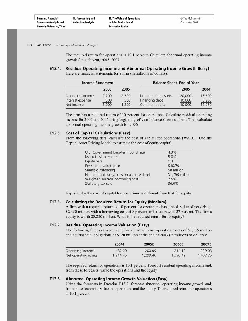
Penman: Financial Statement Analysis and Security Valuation, Third Edition
III. Forecasting and Valuation Analysis
13. The Value of Operations and the Evaluation of Enterprise Ratios
© The McGraw−Hill Companies, 2007
The required return for operations is 10.1 percent. Calculate abnormal operating incomegrowth for each year, 2005–2007.
E13.4. Residual Operating Income and Abnormal Operating Income Growth (Easy)Here are financial statements for a firm (in millions of dollars):
Income Statement Balance Sheet, End of Year
2006 2005 2005 2004
Operating income 2,700 2,300 Net operating assets 20,000 18,500Interest expense 800 500 Financing debt 10,000 6,250Net income 1,900 1,800 Common equity 10,000 12,250
The firm has a required return of 10 percent for operations. Calculate residual operatingincome for 2006 and 2005 using beginning-of-year balance sheet numbers. Then calculateabnormal operating income growth for 2006.
E13.5. Cost of Capital Calculations (Easy)From the following data, calculate the cost of capital for operations (WACC). Use theCapital Asset Pricing Model to estimate the cost of equity capital.
U.S. Government long-term bond rate 4.3%Market risk premium 5.0%Equity beta 1.3Per share market price $40.70Shares outstanding 58 millionNet financial obligations on balance sheet $1,750 millionWeighted average borrowing cost 7.5%Statutory tax rate 36.0%
Explain why the cost of capital for operations is different from that for equity.
E13.6. Calculating the Required Return for Equity (Medium)A firm with a required return of 10 percent for operations has a book value of net debt of$2,450 million with a borrowing cost of 8 percent and a tax rate of 37 percent. The firm’sequity is worth $8,280 million. What is the required return for its equity?
E13.7. Residual Operating Income Valuation (Easy)The following forecasts were made for a firm with net operating assets of $1,135 millionand net financial obligations of $720 million at the end of 2003 (in millions of dollars):
2004E 2005E 2006E 2007E
Operating income 187.00 200.09 214.10 229.08Net operating assets 1,214.45 1,299.46 1,390.42 1,487.75
The required return for operations is 10.1 percent. Forecast residual operating income and,from these forecasts, value the operations and the equity.
E13.8. Abnormal Operating Income Growth Valuation (Easy)Using the forecasts in Exercise E13.7, forecast abnormal operating income growth and,from these forecasts, value the operations and the equity. The required return for operationsis 10.1 percent.
500 Part Three Forecasting and Valuation Analysis

Penman: Financial Statement Analysis and Security Valuation, Third Edition
III. Forecasting and Valuation Analysis
13. The Value of Operations and the Evaluation of Enterprise Ratios
© The McGraw−Hill Companies, 2007
Chapter 13 The Value of Operations and the Evaluation of Enterprise Price-to-Book Ratios and Price-Earnings Ratios 501
E13.9. Growth, the Cost of Capital, and the Normal P/E Ratio (Hard)Box 13.5 in this chapter demonstrated how stock repurchases and leverage changes can in-crease earnings-per-share growth. Answer the following questions regarding the effect ofthe stock repurchase.
a. Why does the stock repurchase have no effect on the per-share value of the equity?b. Why does forecasted earnings for Year 1 decrease from $10.00 million to $7.50 million?c. Why does forecasted EPS for Year 1 increase while forecasted earnings decrease?d. The required return prior to the stock repurchase was 10 percent. What is the required
return for the equity after the stock repurchase?e. What is the expected residual earnings (on equity) for Year 1 after the repurchase?f. Forecast the value of the equity at the end of Year 1 for both the case with no leverage
and the case with leverage.g. Forecast the P/E at the end of Year 1 for both the case with no leverage and the case
with leverage. Why are they different?
E13.10. Levered and Unlevered P/B and P/E Ratios (Easy)A firm has the following summary balance sheet and income statement (in millions):
Net operating assets $469Net financial obligations 236Common equity $233
Operating income $ 70Net financial expense 14Earnings $ 56
The firm held the same amount of net financial obligations during the whole year for whichthe earnings were reported. The equity of this firm trades at a P/B ratio of 2.9. The firm paysno dividends.
a. Calculate the levered P/E ratio for this firm.b. Caltulate the enterprise P/B and P/E ratios.
E13.11. Levered and Unlevered P/E Ratios (Medium)The following pro forma was prepared for a firm at the end of 2005 (in millions of dollars):
2005A 2006E 2007E 2008E
Net operating assets 1,300 1,300 1,300 1,300Net financial obligations 300 300 300 300Common shareholders’ equity 1,000 1,000 1,000 1,000
Operating income 135 135 135Net financial expense 15 15 15Earnings 120 120 120
The firm has a required return for its operations of 9 percent and a 5 percent after-tax costof debt. Pro forma financial statements after 2008 are forecasted to be similar to those in2008.
a. Forecast the value of the operations and the value of the equity at the end of years 2006to 2008.
b. Forecast the levered and unlevered P/E ratios at the end of years 2006 to 2008. Makecalculations for both the expected trailing P/E and the forward P/E.
c. Can you infer the required return for equity from the levered P/E ratios?
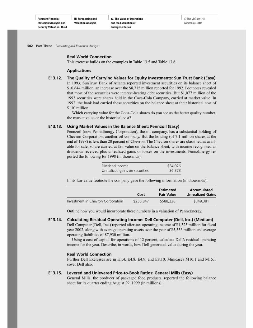
Penman: Financial Statement Analysis and Security Valuation, Third Edition
III. Forecasting and Valuation Analysis
13. The Value of Operations and the Evaluation of Enterprise Ratios
© The McGraw−Hill Companies, 2007
Real World ConnectionThis exercise builds on the examples in Table 13.5 and Table 13.6.
Applications
E13.12. The Quality of Carrying Values for Equity Investments: Sun Trust Bank (Easy)In 1993, SunTrust Bank of Atlanta reported investment securities on its balance sheet of$10,644 million, an increase over the $8,715 million reported for 1992. Footnotes revealedthat most of the securities were interest-bearing debt securities. But $1,077 million of the1993 securities were shares held in the Coca-Cola Company, carried at market value. In1992, the bank had carried these securities on the balance sheet at their historical cost of$110 million.
Which carrying value for the Coca-Cola shares do you see as the better quality number,the market value or the historical cost?
E13.13. Using Market Values in the Balance Sheet: Pennzoil (Easy)Pennzoil (now PennzEnergy Corporation), the oil company, has a substantial holding ofChevron Corporation, another oil company. But the holding (of 7.1 million shares at theend of 1998) is less than 20 percent of Chevron. The Chevron shares are classified as avail-able for sale, so are carried at fair value on the balance sheet, with income recognized asdividends received plus unrealized gains or losses on the investments. PennzEnergy re-ported the following for 1998 (in thousands):
Dividend income $34,026Unrealized gains on securities 36,373
In its fair-value footnote the company gave the following information (in thousands):
Estimated AccumulatedCost Fair Value Unrealized Gains
Investment in Chevron Corporation $238,847 $588,228 $349,381
Outline how you would incorporate these numbers in a valuation of PennzEnergy.
E13.14. Calculating Residual Operating Income: Dell Computer (Dell, Inc.) (Medium)Dell Computer (Dell, Inc.) reported after-tax operating income of $1,325 million for fiscalyear 2002, along with average operating assets over the year of $5,553 million and averageoperating liabilities of $7,930 million.
Using a cost of capital for operations of 12 percent, calculate Dell’s residual operatingincome for the year. Describe, in words, how Dell generated value during the year.
Real World ConnectionFurther Dell Exercises are in E1.4, E4.8, E4.9, and E8.10. Minicases M10.1 and M15.1cover Dell also.
E13.15. Levered and Unlevered Price-to-Book Ratios: General Mills (Easy)General Mills, the producer of packaged food products, reported the following balancesheet for its quarter ending August 29, 1999 (in millions):
502 Part Three Forecasting and Valuation Analysis
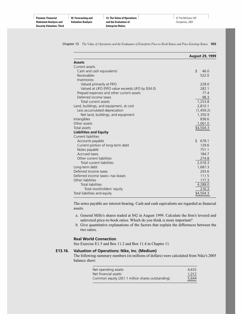
Penman: Financial Statement Analysis and Security Valuation, Third Edition
III. Forecasting and Valuation Analysis
13. The Value of Operations and the Evaluation of Enterprise Ratios
© The McGraw−Hill Companies, 2007
August 29, 1999
AssetsCurrent assets
Cash and cash equivalents $ 46.0Receivables 522.0Inventories
Valued primarily at FIFO 228.0Valued at LIFO (FIFO value exceeds LIFO by $34.0) 282.1
Prepaid expenses and other current assets 77.4Deferred income taxes 98.3
Total current assets 1,253.8Land, buildings, and equipment, at cost 2,810.1
Less accumulated depreciation (1,459.2)Net land, buildings, and equipment 1,350.9
Intangibles 838.6Other assets 1,061.0Total assets $4,504.3Liabilities and EquityCurrent liabilities
Accounts payable $ 678.1Current portion of long-term debt 129.6Notes payable 751.1Accrued taxes 184.7Other current liabilities 274.8
Total current liabilities 2,018.3Long-term debt 1,687.3Deferred income taxes 293.6Deferred income taxes—tax leases 111.5Other liabilities 177.3
Total liabilities 4,288.0Total stockholders’ equity 216.3
Total liabilities and equity $4,504.3
The notes payable are interest-bearing. Cash and cash equivalents are regarded as financialassets.
a. General Mills’s shares traded at $42 in August 1999. Calculate the firm’s levered andunlevered price-to-book ratios. Which do you think is more important?
b. Give quantitative explanations of the factors that explain the differences between thetwo ratios.
Real World ConnectionSee Exercise E1.5 and Box 11.2 and Box 11.4 in Chapter 11.
E13.16. Valuation of Operations: Nike, Inc. (Medium)The following summary numbers (in millions of dollars) were calculated from Nike’s 2005balance sheet:
Net operating assets 4,632Net financial assets 1,012Common equity (261.1 million shares outstanding) 5,644
Chapter 13 The Value of Operations and the Evaluation of Enterprise Price-to-Book Ratios and Price-Earnings Ratios 503
Penman: Financial Statement Analysis and Security Valuation, Third Edition
III. Forecasting and Valuation Analysis
13. The Value of Operations and the Evaluation of Enterprise Ratios
© The McGraw−Hill Companies, 2007
Analysts were forecasting $5.08 in earnings per share for 2006. Nike’s after-tax return onits net financial assets is 3.2 percent and its required return for operations is 8.6 percent.
a. What return on net operating assets (RNOA) are analysts implicitly forecasting for2006?
b. Value a share of Nike on the assumption that the forecasted 2006 RNOA will continueindefinitely and residual operating income (ReOI) and net operating assets will grow at4 percent per year.
c. Repeat the valuation from forecasts of abnormal operating income.d. What is the value of Nike’s operations with these forecasting assumptions?e. If forecasted RNOA is expected to be constant in the future, how can residual operat-
ing income grow?f. Calculate Nike’s levered P/B ratio and also its enterprise P/B ratio. Show how they
relate to each other.g. Calculate Nike’s levered forward P/E and its enterprise forward P/E. Show how they
relate to each other. Explain why one is higher than the other.h. In the press release announcing 2005 results, Nike made the following statements:
During the fourth quarter, the Company purchased a total of 1,853,500 shares for ap-proximately $152.7 million in conjunction with the Company’s four-year, $1.5 billionshare repurchase program that was approved by the Board of Directors in June 2004.To date, the Company has repurchased a total of 6,924,400 shares under this program.
Discuss how the stock repurchases will affect forecasts of future operating income andearnings per share.
Real World ConnectionExercises E2.13, E6.6, E8.8, E8.11, E14.11, E15.10, and E18.5 deal with Nike as do Mini-cases M2.1, M7.1, and M11.2. Also see the coverage of Nike in the BYOAP feature on thebook’s Web site.
504 Part Three Forecasting and Valuation Analysis
Penman: Financial Statement Analysis and Security Valuation, Third Edition
III. Forecasting and Valuation Analysis
13. The Value of Operations and the Evaluation of Enterprise Ratios
© The McGraw−Hill Companies, 2007
Minicases M13.1
Valuing the Operations and the Investmentsof a Property and Casualty Insurer:Chubb CorporationChubb Corporation is a property and casualty insurance holding company providing insur-ance through its subsidiaries in the United States, Canada, Europe, and parts of LatinAmerica and Asia. Its subsidiaries include Federal, Vigilant, Pacific Indemnity, Great Noth-ern, Chubb National, Chubb Indemnity, Executive Risk Indemnity, Executive Risk Spe-cialty, and Quadrant insurance companies.
The insurance operations are divided into three business units. Chubb CommercialInsurance offers a full range of commercial customer insurance products, including cover-age for multiple peril, casualty, workers compensation, and property and marine. ChubbCommercial Insurance writes policies for niche business through agents and brokers.Chubb Specialty Insurance offers a wide variety of specialized executive protection andprofessional liability products for privately and publicly owned companies, financial insti-tutions, professional firms, and health-care organizations. Chubb Specialty Insurance alsoincludes surety and accident businesses, as well as reinsurance through Chubb Re. ChubbPersonal Insurance offers products for individuals with fine homes and possessions whorequire more coverage choices and higher limits than standard insurance policies.
Before proceeding with this case, you should understand how insurers “make money.”Insurance companies run underwriting operations where they write insurance policies andprocesses and pay claims on those policies. The delay between receipt of premiums andpayment of claims produces a “float,” so they are also involved in investment operationswhere they manage investments in which the float is invested. Accordingly, you see both in-vestment assets and liabilities on the balance sheet as well as assets and liabilites associatedwith insurance. You also see revenues and expenses associated with both activities in theincome statement.
A frequently used measure of property and casualty insurance underwriting results isthe combined loss and expense ratio. This ratio is the sum of the ratio of incurred losses andrelated loss adjustment expenses to premiums earned (the loss ratio) and the ratio of un-derwriting expenses to premiums written (the expense ratio), after reducing both premiumamounts by dividends to policyholders. When the combined ratio is under 100 percent,underwriting results are generally considered profitable; when the combined ratio is over100 percent, underwriting results are generally considered unprofitable.
Chubb’s ratios for years 1999–2004 are below. In their discussion of results for 2004,management stated that “underwriting results were highly profitable in 2004 comparedwith modestly profitable results in 2003 and unprofitable results in 2002.” The lower resultsis 2003 were due to large asbestos and toxic waste claims, but even excluding these, thecombined loss and expense ratio would have been 97.5 percent. The 2001 ratio was affectedby claims arising from the September 11 attack in New York and surety bond losses relat-ing to the Enron bankruptcy. Without these claims, the combined ratio would have been100.5 percent.
Chapter 13 The Value of Operations and the Evaluation of Enterprise Price-to-Book Ratios and Price-Earnings Ratios 505

Penman: Financial Statement Analysis and Security Valuation, Third Edition
III. Forecasting and Valuation Analysis
13. The Value of Operations and the Evaluation of Enterprise Ratios
© The McGraw−Hill Companies, 2007
2004 2003 2002 2001 2000 1999
Loss ratio 63.1% 67.6% 75.4% 80.8% 67.5% 70.3%Expense ratio 29.2 30.4 31.3 32.6 32.9 32.5Combined ratio 92.3% 98.0% 106.7% 113.4% 100.4% 102.8%
These ratios give a good indication of the profitability of the insurance operations, butwe need dollar numbers to get to the valuation implications. Further, they do not considerthe performance of the investment operations. Chubb’s balance sheets for 2003 and 2004are in Exhibit 9.15 in Chapter 9 as part of the Chubb case M9.2 there. Its 2004 incomestatement is also given, along with a statement of comprehensive income that Chubb re-ports outside both the equity statement and the income statement. If you worked case M9.2,you will have reformulated these statements. If not, do so now before you proceed. The re-formulation should capture the way that Chubb carries out its business operations, with theanalysis of the profitability of the business in mind. In particular, make sure you distinguishthe underwriting operations from the investment operations. Chubb has some relativelysmall real estate operations. Group these with the underwriting operations. The firm’s statu-tory tax rate is 35 percent, but note that tax-exempt securities account for $174 million ofinvestment income.
Chubb’s loss and expense ratios indicate that 2004 was a very good year. The stockprice, under the ticker CB, rose from $68 to $82 on these results. You are required to carryout an analysis that challenges this stock price. You do not have the complete informationthat you would like for forecasting, but you will be surprised how far you get simply on thebasis of the financial statement information before you.
As you proceed, also deal with the following:
A. Calculate the residual income from underwriting operations and from the investmentoperations and decide how you will use these numbers for your valuation. Use a re-quired return of 9 percent for the underwriting operations and 6 percent for investmentoperations. Why would the two operations have different required returns?
B. Explain the following feature in your valuation:
1. Investment income
2. Realized investment gains
3. Unrealized appreciation of investments
4. Book value of investments
5. Equity investments
6. Net operating assets
7. Tax allocation
C. Insurance companies are suspected of cherry-picking investments. How did you dealwith this?
D. What features of Chubb’s accounting—and insurers in general—might give you pausein basing your valuation on the financial statements?
E. Would you say that Chubb was creating value for shareholders?
Real World ConnectionMinicase M9.2 in Chapter 9 deals with the reformulation on Chubb Corporation’s financialstatements.
506 Part Three Forecasting and Valuation Analysis

Penman: Financial Statement Analysis and Security Valuation, Third Edition
III. Forecasting and Valuation Analysis
13. The Value of Operations and the Evaluation of Enterprise Ratios
© The McGraw−Hill Companies, 2007
M13.2
A Firm with Implied Value of Operationsof Zero: Comverse Technology, Inc.Comverse Technology Inc. designs and manufactures computer and telecommunicationssystems for multimedia communications. The company’s subsidiaries are Comverse Inc.,Verint Systems Inc., and Ulticom, Inc. The company’s products are used in a broad rangeof applications by wireless and wireline telecommunications network operators and serviceproviders, call centers, and other public and commercial organizations worldwide.
When the telecom sector collapsed in 2001 and 2002, the firm’s sales and profitsdeclined considerably. For its second quarter ended July 31, 2002, Comverse reported earn-ings of only 2 cents per share, down from 15 cents from the same quarter of the previousyear. The balance sheet for the quarter is below.
COMVERSE TECHNOLOGY INC. AND SUBSIDIARIESCondensed Consolidated Balance Sheets (in thousands, except share data)
January 31, 2002 July 31, 2002
AssetsCurrent Assets:
Cash and cash equivalents $1,361,862 $ 1,391,705Bank time deposits and short-term investments 530,622 415,294Accounts receivable, net 371,928 291,169Inventories 56,024 51,055Prepaid expenses and other current assets 76,667 69,344
Total current assets 2,397,103 2,218,567Property and equipment, net 181,761 175,667Other assets 125,299 139,581Total assets $2,704,163 $ 2,533,815
Liabilites and Stockholders’ Equity:Current Liabilities:
Accounts payable and accrued expenses $ 322,402 $ 255,998Advance payments from customers 39,576 44,563Other current liabilities 4,875 47,051
Total current liabilities 366,853 347,612Convertible debentures 600,000 434,000Liability for severance pay 9,772 9,421Other liabilities 49,827 9,997Total liabilities 1,026,452 801,030Minority interest 61,303 80,139
Stockholders’ Equity:Common stock, $0.10 per value—authorized,
600,000,000 shares issued and outstanding,186,248,350 and 186,981,198 18,625 18,698
Additional paid-in capital 1,018,232 1,073,681Retained earnings 574,763 555,110Accumulated other comprehensive income 4,788 5,157
Total stockholders’ equity 1,616,408 1,652,646Total liabilities and stockholders’ equity $2,704,163 $ 2,533,815
Chapter 13 The Value of Operations and the Evaluation of Enterprise Price-to-Book Ratios and Price-Earnings Ratios 507

Penman: Financial Statement Analysis and Security Valuation, Third Edition
III. Forecasting and Valuation Analysis
13. The Value of Operations and the Evaluation of Enterprise Ratios
© The McGraw−Hill Companies, 2007
After the second quarter report was published, shares of the firm traded at $7 each.Based on the July 2002 balance sheet, calculate the following:
A. Book value per share.
B. Net financial assets per share.
C. The unlevered price-to-book ratio.
D. The ratio of equity price to net financial assets.
What value is the market placing on the operations?You will observe that the shares are trading at less than the amount of cash that the firm
is holding. Analysts often consider this situation as a certain case of underpricing. Whatother information would you like to have before you purchase this stock?
508 Part Three Forecasting and Valuation Analysis