Chap. 23 FIRM SUPPLY
51
Engineering Economic Analysis 2019 SPRING Prof. D. J. LEE, SNU Chap. 23 FIRM SUPPLY
Transcript of Chap. 23 FIRM SUPPLY

Engineering Economic Analysis2019 SPRING
Prof. D. J. LEE, SNU
Chap. 23
FIRM SUPPLY
Market Environments
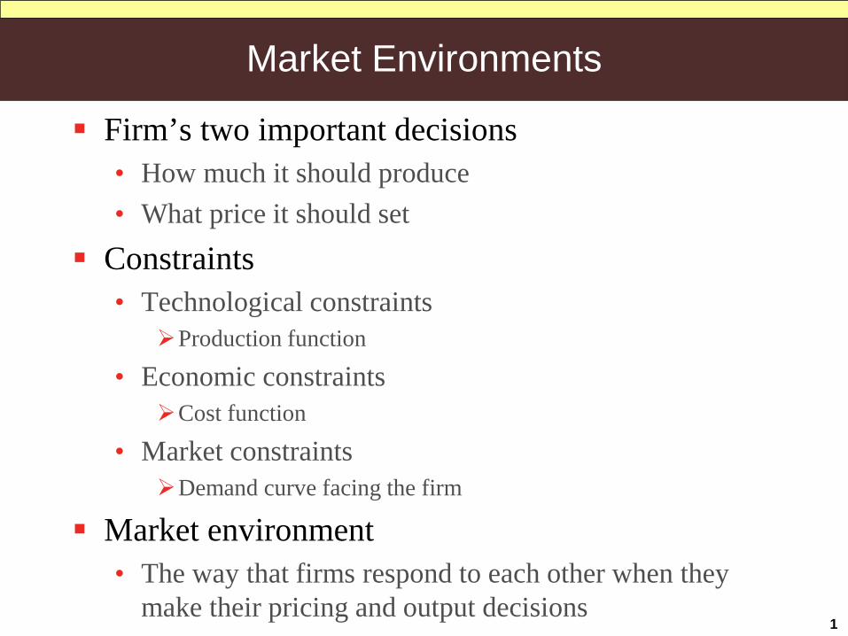
Firm’s two important decisions• How much it should produce• What price it should set
Constraints• Technological constraints
Production function
• Economic constraintsCost function
• Market constraintsDemand curve facing the firm
Market environment• The way that firms respond to each other when they
make their pricing and output decisions1

Pure competition
Market is purely competitive if each firm assumes that the market price is independent of its own level of output• An industry of many firms that produce an identical
good, and that each firm is a small part of the market• Only worry about how much output it produces
(supply)• Price taker
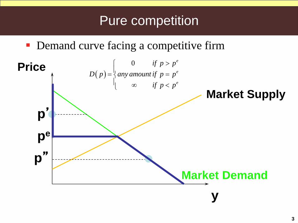
Demand curve facing a competitive firm• Let pe be the market price
2
( )0 e
e
e
if p pD p any amount if p p
if p p
>= = ∞ <
Pure competition
Demand curve facing a competitive firm
3
y
Price
Market Supply
pe
p’
p”
Market Demand
( )0 e
e
e
if p pD p any amount if p p
if p p
>= = ∞ <

Pure competition
Demand curve facing a competitive firm
4
y
Price
pe
( )0 e
e
e
if p pD p any amount if p p
if p p
>= = ∞ <
• Horizontal, infinitely elastic demand

Pure competition
What does it mean to say that an individual firm is “small relative to the industry”?
Price
y
Firm’s MCFirm’s demand
curvepe
• The individual firm’s capacity to supply can cover only a small part of the total quantity demanded at the market price
Supply decision of a competitive firm
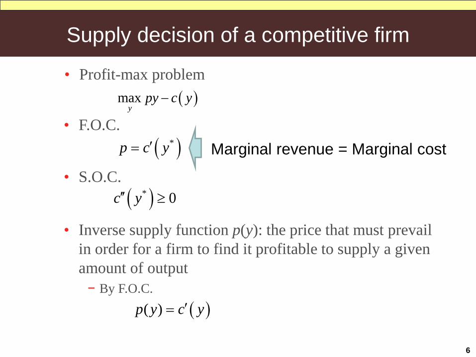
• Profit-max problem
6
( )maxy
py c y−
• F.O.C. ( )*p c y′=
• Inverse supply function p(y): the price that must prevail in order for a firm to find it profitable to supply a given amount of output− By F.O.C.
( )* 0c y′′ ≥
Marginal revenue = Marginal cost
• S.O.C.
( )( )p y c y′=

Supply decision of a competitive firm
Supply function y(p): the profit-maximizing output at price of p
7
• Whatever the level of market price p, the competitive firm will choose a level of output where ( )( )p c y p′=
( )( ) 0c y p′′ ≥• In addition, by S.O.C., the firm will supply the output
which satisfy
Therefore, the supply curve of the competitive firm is the upward sloping part of its marginal cost curve!
( )( )( )( ) ( )
( )
Differentiating F.O.C. ( ) w.r.t.
1
By S.O.C. ( ) 0 0
p c y p p
c y p y p
c y y p
′≡
′′ ′=
′′ ′> ⇒ >
Supply decision of a competitive firm
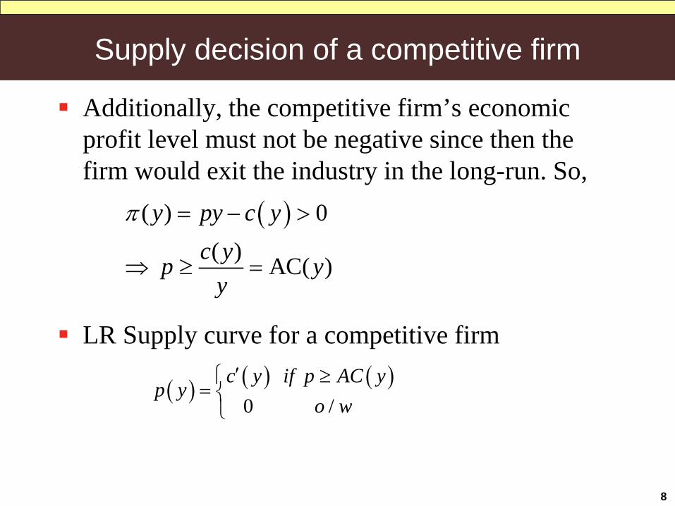
Additionally, the competitive firm’s economic profit level must not be negative since then the firm would exit the industry in the long-run. So,
8
( )( ) 0( ) AC( )
y py c yc yp y
y
π = − >
⇒ ≥ =
LR Supply curve for a competitive firm
( ) ( ) ( ) 0 /
c y if p AC yp y
o w′ ≥
=

Supply decision of a competitive firm
9
MC(y)
AC(y)
y
Price/cost
p > AC(y)
Exit price
The firm’s long-runsupply curve

Supply decision of a competitive firm
SR Supply curve considering SR cost curve• Let
10
( ) ( )vc y c y F= +
• Then ( ) ( )( )vp y p c y p Fπ = ⋅ − −
• Producing a positive output (y >0) is profitable compared with the case of producing zero if
( ) ( )( )( )( )( ) ( )( )
v
v
p y p c y p F F
c y pp AVC y p
y p
⋅ − − ≥ −
≥ =
SR Supply curve for a competitive firm
( ) ( ) ( ) 0 /
c y if p AVC yp y
o w′ ≥
=
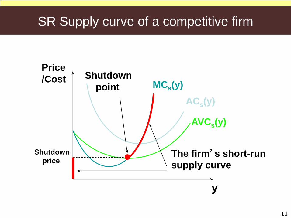
SR Supply curve of a competitive firm
11
AVCs(y)
ACs(y)MCs(y)
The firm’s short-runsupply curve
Shutdownpoint
Price/Cost
y
Shutdownprice

SR Supply decision of a competitive firm
12
Shut-down is not the same as exit. Shutting-down means producing no output (but
the firm is still in the industry and suffers its fixed cost because exit is impossible in the short-run).
Exiting means leaving the industry, which the firm can do only in the long-run.

Profits and Producer’s surplus
13
Producer’s surplus• Supply curve measures the amount that will be supplied
at each price• The area above the supply curve measures the surplus
enjoyed by the suppliers of a good
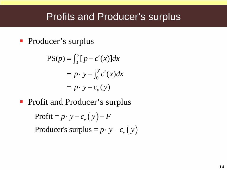
Profits and Producer’s surplus
14
Producer’s surplus
0
0
PS( ) [ ( )]
( )
( )
y
y
v
p p c x dx
p y c x dx
p y c y
′= −
′= ⋅ −
= ⋅ −
∫
∫
Profit and Producer’s surplus
( )( )
Profit =
Producer's surplus = v
v
p y c y F
p y c y
⋅ − −
⋅ −
Profits and Producer’s surplus
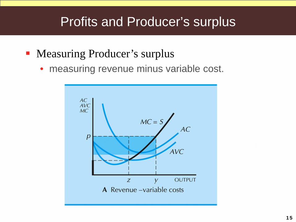
15
Measuring Producer’s surplus• measuring revenue minus variable cost.
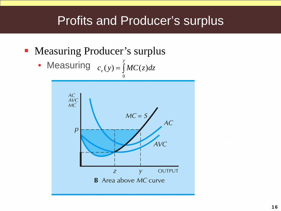
Profits and Producer’s surplus
16
Measuring Producer’s surplus• Measuring
0( ) ( )
y
vc y MC z dz= ∫

Profits and Producer’s surplus
17
Measuring Producer’s surplus• Measuring the box up until output z (area R) and
then uses the area above the marginal cost curve (area T).
Supply curve
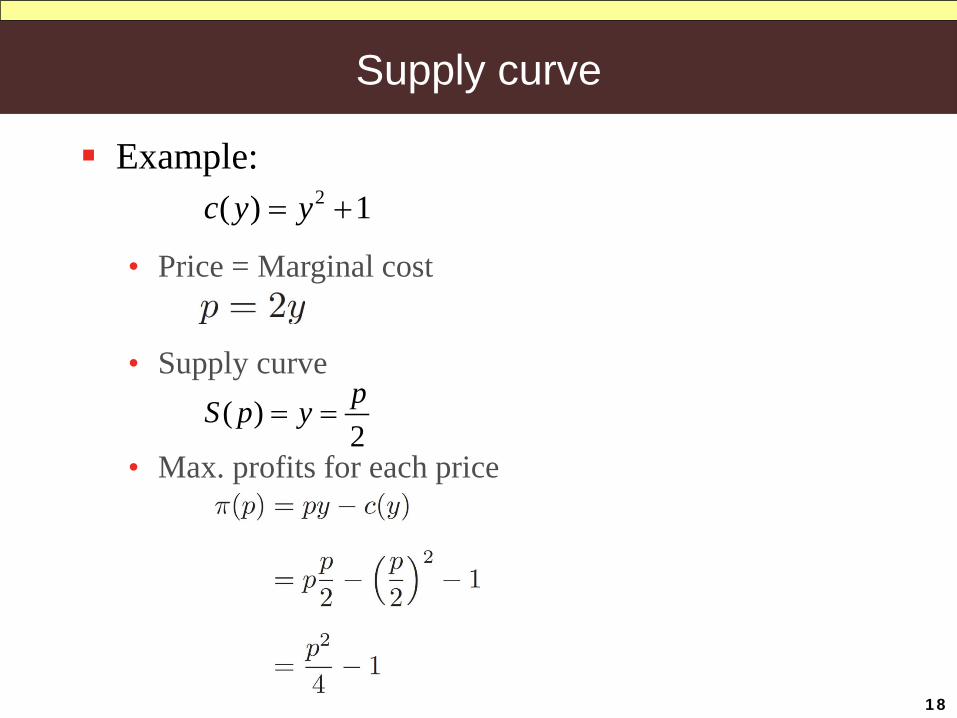
18
Example:2( ) 1c y y= +
• Price = Marginal cost
• Supply curve ( )
2pS p y= =
• Max. profits for each price
Supply curve
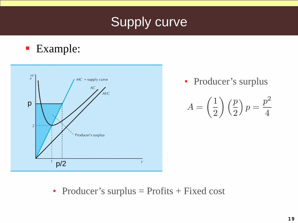
19
Example:
• Producer’s surplus
• Producer’s surplus = Profits + Fixed cost
p
p/2
Engineering Economic Analysis2019 SPRING
Prof. D. J. LEE, SNU
Chap. 24
INDUSTRY SUPPLY
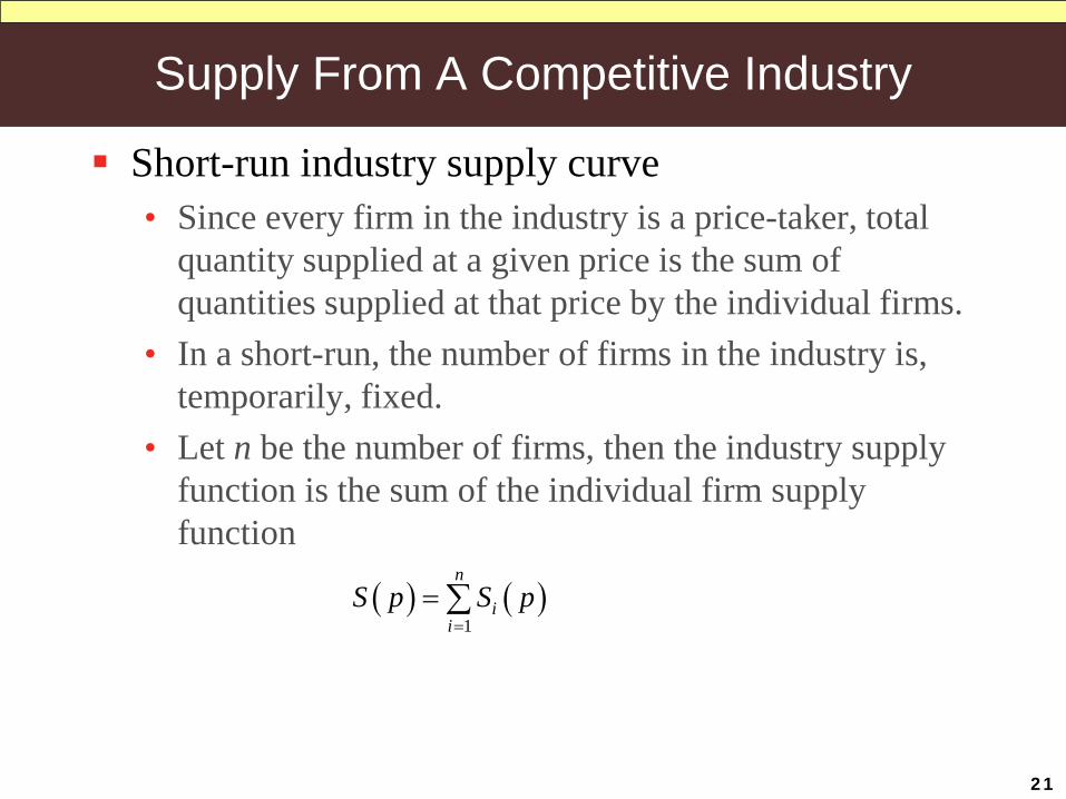
Supply From A Competitive Industry
Short-run industry supply curve• Since every firm in the industry is a price-taker, total
quantity supplied at a given price is the sum of quantities supplied at that price by the individual firms.
• In a short-run, the number of firms in the industry is, temporarily, fixed.
• Let n be the number of firms, then the industry supply function is the sum of the individual firm supply function
21
( ) ( )1
n
ii
S p S p=
= ∑
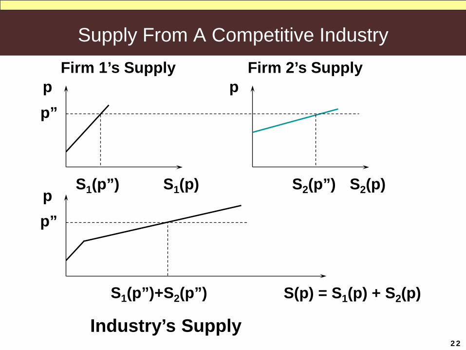
Supply From A Competitive Industry
p
S1(p)
p
S2(p)p
S(p) = S1(p) + S2(p)
p”
p”
S1(p”)
S1(p”)+S2(p”)
S2(p”)
Firm 1’s Supply Firm 2’s Supply
Industry’s Supply22

Supply From A Competitive Industry
23
Example: n firms with common cost ( ) 2 1c y y= +
• Inverse supply function ( ) ( ) 2p y MC y y= =
• Individual supply function ( )2ipS p =
• Industry supply function ( ) ( )1 2
n
ii
pS p S p Y n=
= = =∑
• Inverse industry supply function 2( )p Y Yn
=
− Note that ( ) 2 ( ) for all 0MC y y AVC y y y= ≥ = ≥
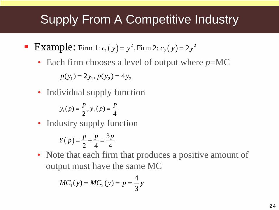
Supply From A Competitive Industry
24
Example:• Each firm chooses a level of output where p=MC
( ) ( )2 21 2Firm 1: ,Firm 2: 2c y y c y y= =
• Note that each firm that produces a positive amount of output must have the same MC
1 1 2 2( ) 2 , ( ) 4p y y p y y= =
• Individual supply function
1 2( ) , ( )2 4p py p y p= =
• Industry supply function
( ) 32 4 4p p pY p = + =
1 24( ) ( )3
MC y MC y p y= = =

Short-Run Industry Equilibrium
In a short-run, neither entry nor exit can occur.
25
( )( )
: individual 's demand function, 1,...,
: supply function of firm , 1,...,i
j
x p i i n
y p j j m
=
=
• Equilibrium price p*( ) ( )* *
i ji j
x p y p=∑ ∑
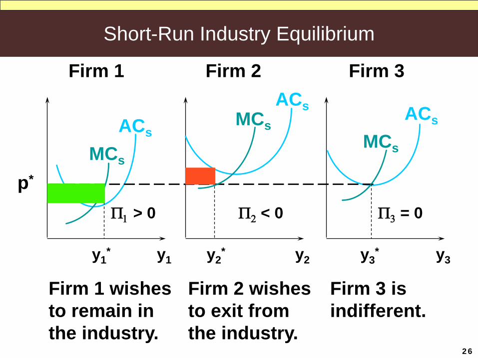
Short-Run Industry Equilibrium
y1 y2 y3
ACs
ACs ACs
MCs
MCsMCs
y1* y2
* y3*
p*
Firm 1 Firm 2 Firm 3
Firm 1 wishesto remain inthe industry.
Firm 2 wishesto exit fromthe industry.
Firm 3 isindifferent.
Π1 > 0 Π2 < 0 Π3 = 0
26
Short-Run Industry Equilibrium
In a short-run, neither entry nor exit can occur.
27
( )( )
: individual 's demand function, 1,...,
: supply function of firm , 1,...,i
j
x p i i n
y p j j m
=
=
• Equilibrium price p*( ) ( )* *
i ji j
x p y p=∑ ∑
Consequently, in a short-run equilibrium, some firms may earn positive economics profits, others may suffer economic losses, and still others may earn zero economic profit

Short-Run Industry Equilibrium
Relationship between SR equilibrium price and the number of firms in a competitive market
28
• Let X(p) be the arbitrary industry demand function and y(p) is a common supply function of individual n firms in a competitive market
• Equilibrium condition: X(p)=ny(p)
• Regard p as an implicit function of n, i.e., p(n)
• Differentiating Eq. condition X(p(n))=ny(p(n)) w.r.t. n( ) ( ) ( ) ( )
( ) ( )( ) ( )
( )X p p n y p n y p p n
y pp n
X p n y p
′ ′ ′ ′= + ⋅
′∴ =′ ′− ⋅
( ) ( ) ( )Since 0, 0 0X p y p p n′ ′ ′< > ⇒ <
As the number of firms increases, SR equil. price decreases

Entry & Long-Run Equilibrium
In the long-run, every firm now in the industry is free to exit and firms now outside the industry are free to enter.
The industry’s long-run supply function must account for entry and exit as well as for the supply choices of firms that choose to be in the industry.• Positive economic profit induces entry.• Economic profit is positive when p* > min AC(y).• Entry increases the number of firms, causing p* to fall.
(dp*/dn<0)• When does entry cease?
29
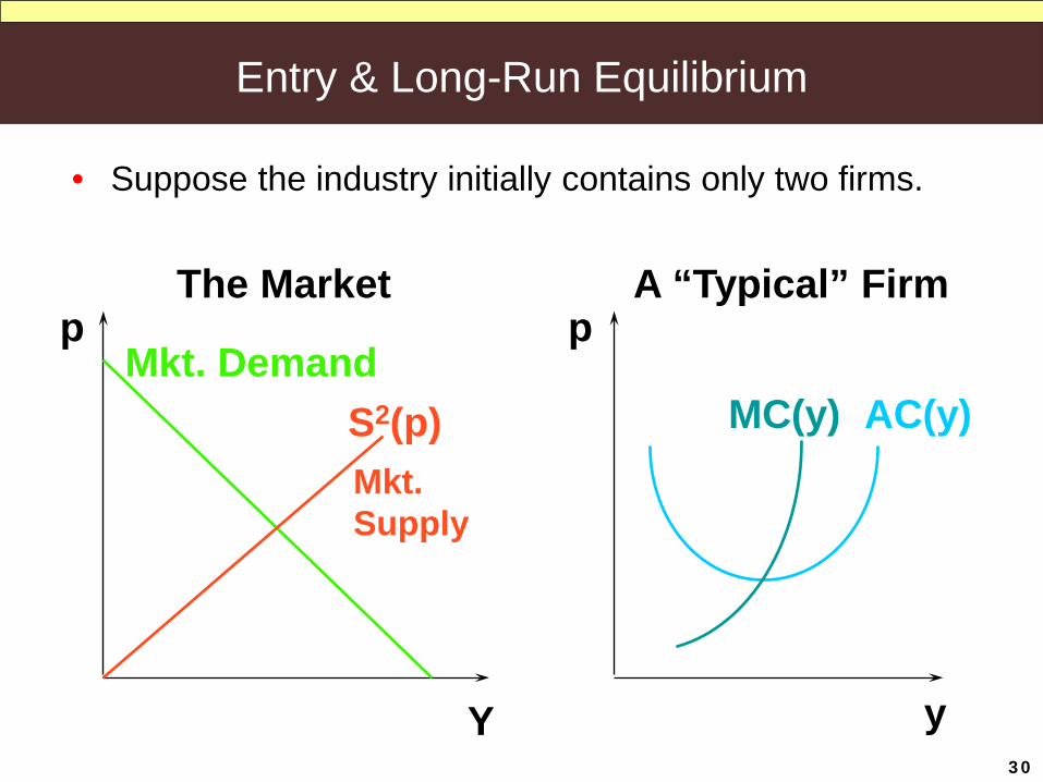
Entry & Long-Run Equilibrium
S2(p)Mkt. Demand
AC(y)MC(y)
y
A “Typical” FirmThe Marketp p
Y
Mkt.Supply
30
• Suppose the industry initially contains only two firms.
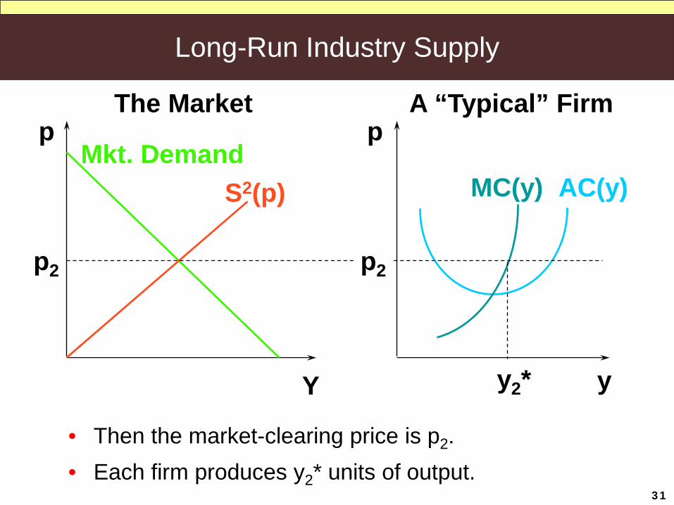
Long-Run Industry Supply
S2(p)Mkt. Demand
AC(y)MC(y)
y
A “Typical” FirmThe Marketp p
Y
p2 p2
• Then the market-clearing price is p2.
31
y2*
• Each firm produces y2* units of output.
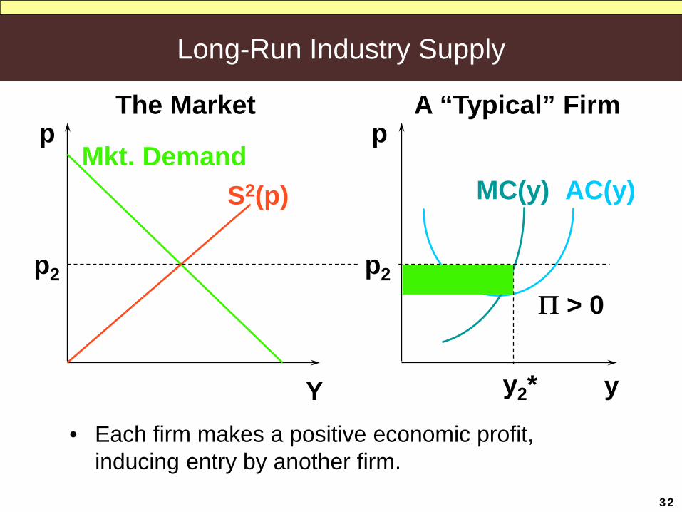
Long-Run Industry Supply
S2(p)Mkt. Demand
AC(y)MC(y)
y
A “Typical” FirmThe Marketp p
Y
p2 p2
y2*
Π > 0
• Each firm makes a positive economic profit, inducing entry by another firm.
32

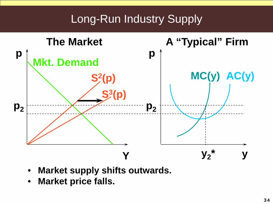
Long-Run Industry Supply
S2(p)S3(p)
Mkt. DemandAC(y)MC(y)
y
A “Typical” FirmThe Marketp p
Y
p2 p2
• Market supply shifts outwards.
y2*
33
Long-Run Industry Supply
S2(p)S3(p)
Mkt. DemandAC(y)MC(y)
y
A “Typical” FirmThe Marketp p
Y
p2 p2
• Market supply shifts outwards.• Market price falls.
y2*
34
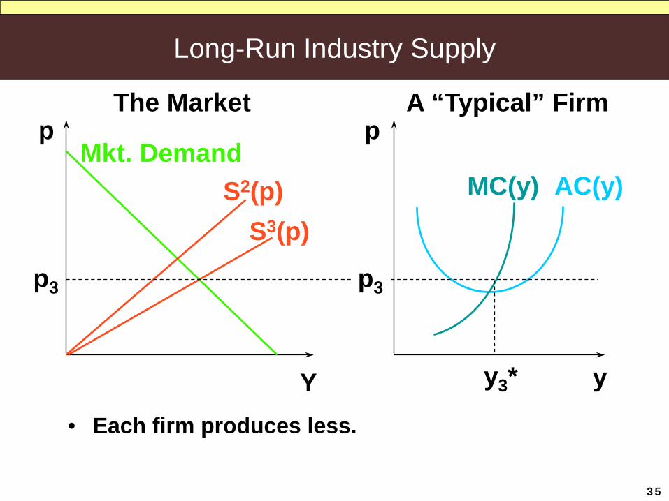
Long-Run Industry Supply
S2(p)S3(p)
Mkt. DemandAC(y)MC(y)
y
A “Typical” FirmThe Marketp p
Y
p3
• Each firm produces less.
y3*
p3
35
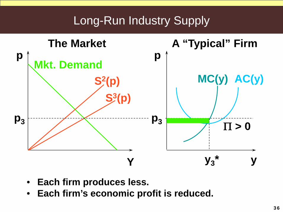
Long-Run Industry Supply
S2(p)S3(p)
Mkt. DemandAC(y)MC(y)
y
A “Typical” FirmThe Marketp p
Y
p3
• Each firm produces less.• Each firm’s economic profit is reduced.
y3*
p3 Π > 0
36

Long-Run Industry Supply
S3(p)
Mkt. DemandAC(y)MC(y)
y
A “Typical” FirmThe Marketp p
Y
p3
• Each firm’s economic profit is still positive.Will another firm enter?
y3*
p3 Π > 0
37
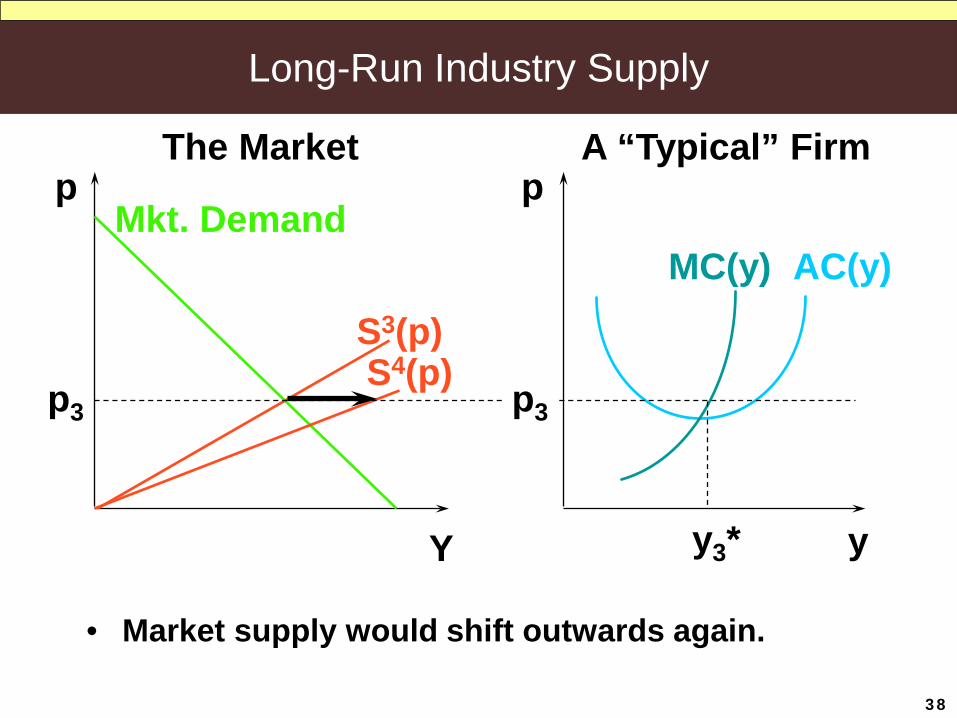
Long-Run Industry Supply
S4(p)S3(p)
Mkt. DemandAC(y)MC(y)
y
A “Typical” FirmThe Marketp p
Y
p3
• Market supply would shift outwards again.
y3*
p3
38

Long-Run Industry Supply
S4(p)S3(p)
Mkt. DemandAC(y)MC(y)
y
A “Typical” FirmThe Marketp p
Y
p3
• Market supply would shift outwards again.• Market price would fall again.
y3*
p3
39

Long-Run Industry Supply
S4(p)S3(p)
Mkt. DemandAC(y)MC(y)
y
A “Typical” FirmThe Marketp p
Y
p4
• Each firm would produce less again.
y4*
p4
40
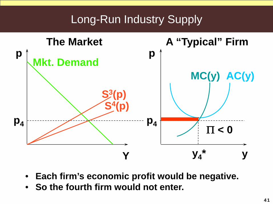
Long-Run Industry Supply
S4(p)S3(p)
Mkt. DemandAC(y)MC(y)
y
A “Typical” FirmThe Marketp p
Y
p4
• Each firm’s economic profit would be negative. • So the fourth firm would not enter.
y4*
Π < 0p4
41

Long-Run Industry Supply
The long-run number of firms in the industry is the largest number for which the market price is at least as large as min AC(y).
( ) 2 1c y y= +
• Break-even level of output is p=AC(y)
• Since p=MC(y) in an equilibrium of competitive market, the break-even output is where p=AC(y)=MC(y)
( )
12 1
1 2
y y yy
Then p MC
= + ⇒ =
= =
• Thus firms will enter the industry as long as they will not drive the equilibrium price below 2
Example: cost function
42
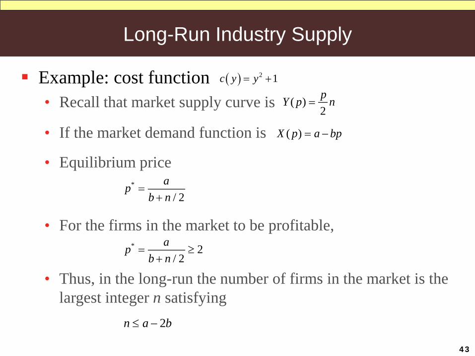
Long-Run Industry Supply
Example: cost function
• If the market demand function is
• Recall that market supply curve is
• Equilibrium price
( ) 2 1c y y= +
( ) 2pY p n=
( ) X p a bp= −
2n a b≤ −
*
/ 2ap
b n=
+
• For the firms in the market to be profitable, * 2
/ 2ap
b n= ≥
+
• Thus, in the long-run the number of firms in the market is the largest integer n satisfying
43

Long-Run Supply Curve
• The competitive industry’s long-run supply curve is horizontal at min AC(y).
AC(y)
MC(y)
y
A “Typical” FirmThe MarketLong-RunSupply Curve
p p
Y y*
44

Long-Run Supply Curve
Now market demand is large enough to sustain only two firms in the industry.
S2(p)Mkt. Demand
AC(y)MC(y)
y
A “Typical” FirmThe Marketp p
Y
p2’
y2*
p2’
45

Long-Run Supply Curve
• Suppose that market demand increases, then the market price rises, each firm produces more, and earns a higher profit.
S2(p)
S3(p)
Mkt. DemandAC(y)MC(y)
y
A “Typical” FirmThe Marketp p
Y y2*
p2” p2”
• Will the 3rd firm enter?46
No! since negative profits.

Long-Run Supply Curve• As market demand increases further, the market price rises
further, the two incumbent firms each earn still higher economic profits -- until the 3rd firm becomes indifferent between entering and staying out.
S2(p)
S3(p)
Mkt. DemandAC(y)MC(y)
y
A “Typical” FirmThe Marketp p
Y y2*
p2’” p2’”
The only relevant part of the short-runsupply curve for n = 2 firms in the industry.
47

Long-Run Supply Curve
• How much further can market demand increase before a fourth firm enters the industry?
S3(p)
Mkt. Demand
AC(y)MC(y)
y
A “Typical” FirmThe Marketp p
Y y3*
S4(p)p3’ p3’
The only relevant part of the short-runsupply curve for n = 3 firms in the industry.
48
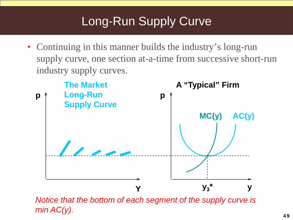
Long-Run Supply Curve
• Continuing in this manner builds the industry’s long-run supply curve, one section at-a-time from successive short-run industry supply curves.
AC(y)MC(y)
y
A “Typical” FirmThe MarketLong-RunSupply Curve
p p
Y y3*Notice that the bottom of each segment of the supply curve is min AC(y).
49

Long-Run Supply Curve
• In the long-run, if there are a reasonable number of firms in the industry(or as firms become sufficiently small), the industry’s long-run supply curve is horizontal at min AC(y).
AC(y)
MC(y)
y
A “Typical” FirmThe MarketLong-RunSupply Curve
p p
Y y*50