Chaos, Fractals and Statistics Sangit Chatterjee; Mustafa ...cshalizi/462/readings/Chaos,...

Chaos, Fractals and Statistics

Sangit Chatterjee; Mustafa R. Yilmaz

Statistical Science, Vol. 7, No. 1. (Feb., 1992), pp. 49-68.

Stable URL:

http://links.jstor.org/sici?sici=0883-4237%28199202%297%3A1%3C49%3ACFAS%3E2.0.CO%3B2-5

Statistical Science is currently published by Institute of Mathematical Statistics.

Your use of the JSTOR archive indicates your acceptance of JSTOR's Terms and Conditions of Use, available athttp://www.jstor.org/about/terms.html. JSTOR's Terms and Conditions of Use provides, in part, that unless you have obtainedprior permission, you may not download an entire issue of a journal or multiple copies of articles, and you may use content inthe JSTOR archive only for your personal, non-commercial use.

Please contact the publisher regarding any further use of this work. Publisher contact information may be obtained athttp://www.jstor.org/journals/ims.html.

Each copy of any part of a JSTOR transmission must contain the same copyright notice that appears on the screen or printedpage of such transmission.

The JSTOR Archive is a trusted digital repository providing for long-term preservation and access to leading academicjournals and scholarly literature from around the world. The Archive is supported by libraries, scholarly societies, publishers,and foundations. It is an initiative of JSTOR, a not-for-profit organization with a mission to help the scholarly community takeadvantage of advances in technology. For more information regarding JSTOR, please contact [email protected].

http://www.jstor.orgSat Jan 5 15:23:41 2008


http://www.jstor.org/about/terms.html

http://www.jstor.org/journals/ims.html

Statistical Science 1992,Vol. 7 , No.1, 49-121

Chaos, Fractals and Statistics Sangit Chatterjee and Mustafa R. Yilmaz

Abstract. We review a wide variety of applications in different branches of sciences arising from the study of dynamical systems. The emergence of chaos and fractals from iterations of simple difference equations is discussed. Notions of phase gpace, contractive mapping, attractor, invariant density and the relevance of ergodic theory for studying dynamical systems are reviewed. Various concepts of dimensions and their relationships are studied, and their use in the measurement of chaotic phenomena is investigated. We discuss the implications of the growth of nonlinear science on paradigms of model building in the tradition of classical statistics. The role that statistical science can play in future developments of nonlinear science and its possible impact on the future development of statistical science itself are addressed.

Key words and phrases: Autonomous systems, dimensions, dynamical systems, ergodic theory, iterations, phase space, strange attractors, time series.

. . . if we conceive of an intelligence which at a Poincar6 (1899) and his investigation of planetary given instant comprehends all the relations of dynamics. Deeply rooted in fluid mechanics, where the entities of the universe, it could state the fluid flow is modeled by differential equations, the respective positions, motions and general af- main purpose of the area of nonlinear dynamics is fects of all these entities at any time in the past to describe complex physical processes in terms of or future. deterministic models. The renewal of interest in

this area in recent decades is because of the sur- prising finding that very simple deterministic mod-

Laplace (1776) els of dynamical systems can yield unpredictable behavior that exhibits the characteristics of a ran-dom process. This finding has greatly widened the

. . . but it is not always so; it may happen that interest in the area because of its relevance to the small differences in the initial conditions pro- study of time series data, a pursuit that has long duce very great ones in the final phenomena. A been of concern to economists and statisticians, as small error in the former will produce a large well as physical scientists. one in the later. Prediction becomes impossible. It should be emphasized at the outset that statis-

tics has always been concerned with the study of complex phenomena, and it has been very success- ful in building stochastic models that are capable of describing such phenomena. On the other hand, these stochastic models use randomness as a basic

The last two decades have witnessed a great concept, so that the process under investigation is resurgence of interest in the mathematical study of assumed to be at least partially governed by chance dynamical systems and chaos. The origins of these and associated laws of probability. In contrast, the fields go far back to the end of last century to new area of dynamical systems and chaos offers the

facinating possibility of describing randomness as the result of a known deterministic process. The

Sangit Chatterjee is ~rofessor of Management Sci- question of being able to identify the circumstances ence and Mustafa R. Yilmaz is Associate Professor under which this is possible renders the new area of Management Science at the College of Business, something more than a subject of mere curiosity. Northeastern University, 219 Hayden Hall, 360 At the present time, this question is only beginning Huntington Avenue, Boston, Massachusetts 02115. to be explored.

50 CHAOS

Most of the important early work related to chaos 1.1 Chaos Through Dynamical Systems and fractals occurred in the fields of biology, meteo- rology, physics, chemistry and computer science. This work remained relatively obscure until the early seventies, when an explosion of interest took place in the ensuing years. Although many re-searchers in different fields contributed to this explosion, the work of Lorenz (1963) involving weather prediction is credited by many for popular- izing the study of chaos. Lorenz showed that the trajectory described by a system of simple differential equations can exhibit strange and chaotic behavior, depending on the exact initial conditions [also see Berliner (1992) in this issue]. An example from chemistry was provided by the Belousov-Zhabotinskii (B-Z) reaction in which the concentration of chemical species do not vary mono- tonically with time but instead oscillate, sometimes chaotically, sometimes periodically (Simoyi, Wolf and Swinney, 1982). The literature is now replete with many other examples involving turbulence and chaos covering such diverse fields as physiology, geology, epidemiology, theoretical models of population biology, economics, statistics, logic and philosophy, and every other branch of scientific investigation.

The -useful models obtained from differential topology in catastrophe theory (Thorn, 1975) exhibit some qualitative properties that are also present in models of chaos. Qualitative properties of a system are invariant under differentiable changes of coordinates as opposed to quantitative properties that are invariant only under linear changes of coordinates. Smale (l-967), who generalized the earlier work of Andronov and Pontyagrin, studied structural instability for differentiable dynamical systems for flows whose topology changes if the equations describing the flow are altered slightly. This idea of structural instability is different from an unstable solution of a given equation. The latter is a solution that is sensitive to small changes in the initial condition and provides a starting point for the study of chaos and-nonlinear theory.

The purpose of this paper is to introduce these ideas of this relatively new area to a wider audi- ence in statistics. We believe that access to these ideas will enrich the arsenal of modeling tools available to statisticians, generate new develop-ments in their refinement and, ultimately, facili- tate a better understanding of the processes being studied. We provide a broad range of references for the reader to pursue individual interests in any particular area. However, this listing is necessarily incomplete because of the sheer volume of the existing literature, as well as the ever-increasing amount of research being reported in diverse fields.

A dynamical system is one whose status changes over time. When change can be described in terms of physical movement, it is possible to distinguish between two types of dynamical systems, depending on whether or not the system loses energy due to friction. The presence of friction characterizes most physical processes in nature that are called dissipative dynamical systems, as opposed to con-servative systems, where there is no loss of energy. A dissipative system always approaches an asymptotic or limiting state of motion over time, and it is this limiting behavior that has made dissipative systems the main focus of research. It was discovered in the sixties that the asymptotic movement can exhibit a rich variety of characteristics, including what may appear to be chaotic or random behavior. Two simple examples where the system status is described by a single variable will moti- vate further discussion. In both examples, the system is observed at distinct points in time which, for the moment, will be designated as t = 0,1,. . . .

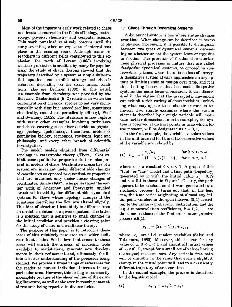
In the first example, the variable x, takes values in the unit interval [O, 11, and two successive values of the variable are related by

~t 10, for0 I X , I w, (1) x , + ~= {

1 - ) ( l - w), for w 5 xt 5 1,

where w is a constant 0 < w < 1. A graph of this "tent" or "hut" model and a time path (trajectory) generated by it with the initial value x, = 0.19 and w = 0.4 is shown in Figure 1.Clearly, the path appears to be random, as if it were generated by a stochastic process. It turns out that, in the long run, the time series originating at almost any initial point wanders in the open interval (0,l) accord- ing to the uniform probability distribution, and the lag k autocorrelation coefficients, k = 1,2,. . . are the same as those of the first-order autoregressive process AR(l),

where ( E , ) are i.i.d. random variables (Sakai and Tokumaru, 1980). Moreover, this is true for any value of w, 0 < w < 1and almost all initial values of x, E (0, I), except for a small set of values having (Lebesgue) measure zero. Any periodic time path will be unstable in the sense that even a slightest change in the initial point will lead to a drastically different trajectory after some time.

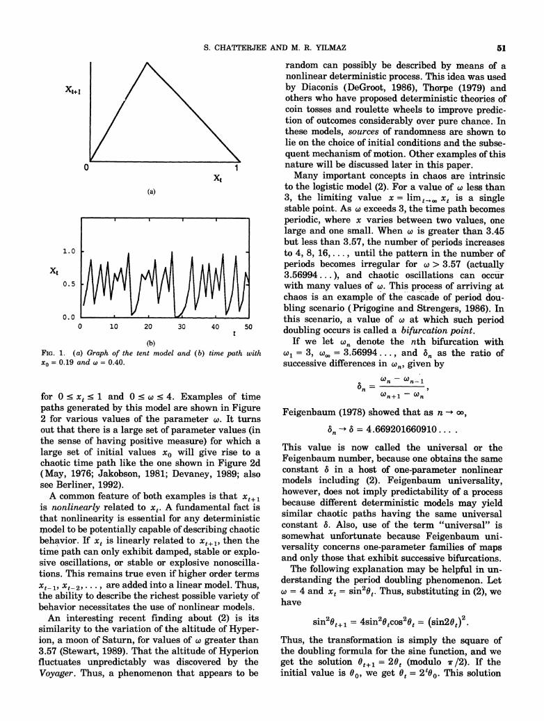
In the second example, the process is described by the logistic model

(2) Xt+.l = wxt(l - x,)

51 AND M.R. YILMAZ

random can possibly be described by means of a nonlinear deterministic process. This idea was used by Diaconis (DeGroot, 1986), Thorpe (1979) and others who have proposed deterministic theories of coin tosses and roulette wheels to improve prediction of outcomes considerably over pure chance. In these models, sources of randomness are shown to lie on the choice of initial conditions and the subsequent mechanism of motion. Other examples of this nature will be discussed later in this paper.

Many important concepts in chaos are intrinsic to the logistic model (2). For a value of w less than 3, the limiting value ,,,lim=x x, is a single

0.0 0 10 20 30 4 0 50

t

(3) FIG. 1. ( a ) Graph of the tent model and ( b ) time path with xo = 0.19 and w = 0.40.

for 0Ix, I1 and 0Iw I 4. Examples of time paths generated by this model are shown in Figure 2 for various values of the parameter w. It turns out that there is a large set of parameter values (in the sense of having positive measure) for which a large set of initial values x, will give rise to a chaotic time path like the one shown in Figure 2d (May, 1976; Jakobson, 1981; Devaney, 1989; also see Berliner, 1992).

A common feature of both examples is that x,+, is nonlinearly related to x,. A fundamental fact is that nonlinearity is essential for any deterministic model to be potentially capable of describing chaotic behavior. If x, is linearly related to x,+,, then the time path can only exhibit damped, stable or explosive oscillations, or stable or explosive nonoscilla- tions. This remains true even if higher order terms x,- ,,x,-,, . . . , are added into a linear model. Thus, the ability to describe the richest possible variety of behavior necessitates the use of nonlinear models.

An interesting recent finding about (2) is its similarity to the variation of the altitude of Hyper- ion, a moon of Saturn, for values of w greater than 3.57 (Stewart, 1989). That the altitude of Hyperion fluctuates unpredictably was discovered by the Voyager. Thus, a phenomenon that appears to be

stable point. As w exceeds 3, the time path becomes periodic, where x varies between two values, one large and one small. When w is greater than 3.45 but less than 3.57, the number of periods increases to 4, 8, 16,. . . , until the pattern in the number of periods becomes irregular for w > 3.57 (actually 3.56994. . . ), and chaotic oscillations can occur with many values of w. This process of arriving at chaos is an example of the cascade of period doubling scenario (Prigogine and Strengers, 1986). In this scenario, a value of w at which such period doubling occurs is called a bifurcation point.

If we let on denote the nth bifurcation with a, = 3, w, = 3.56994.. . , and 6, as the ratio of successive differences in w,, given by

Feigenbaum (1978) showed that as n -+ oo,

This value is now called the universal or the Feigenbaum number, because one obtains the same constant 6 in a host of one-parameter nonlinear models including (2). Feigenbaum universality, however, does not imply predictability of a process because different deterministic models may yield similar chaotic paths having the same universal constant 6. Also, use of the term "universal" is somewhat unfortunate because Feigenbaum universality concerns one-parameter families of maps and only those that exhibit successive bifurcations.

The following explanation may be helpful in understanding the period doubling phenomenon. Let w = 4 and x, = sin26,. Thus, substituting in (2), we have

Thus, the transformation is simply the square of the doubling formula for the sine function, and we get the solution 6,+, = 26, (modulo ?r 12). If the initial value is 00, we get 6, = zt6,. This solution

CHAOS

Time

o= 2.5 t w = 4.0 t

(c) (4 FIG.2. Graph of the logistic model and time paths generated by it for several values of w.

also shows that x , sensitively depends on the initial point O, , so that two initial points that are very close diverge rapidly as t is increased.

The period doubling-scenario is by no means the only route to chaotic behavior. An example where chaos occurs without this phenomenon is given by the tent model (1). A more extreme example is the completely chaotic model discussed by May (1985) and Rogers, Yang and Yip (1986) that exhibits chaotic behavior for all values of some parameter. An attempt to catalog the various possible routes to chaotic system behavior and examples of associated qodels was given by BergB, Pomeau and Vidal (1984). Another good source for dynamical systems resulting from iterates of maps on a real interval is Collet and Eckmann (1980).

The term "chaos" was coined by Li and Yorke (1975), although it was also used by Lorenz (1963) earlier in his study of a system of differential equations in modeling turbulence for study of weather patterns. The popular book by Gleick (1987) gives an excellent historical account of the development of the study of physical chaos starting from the work of Lorenz. The number of more technically oriented books on dynamical systems and chaos has been rapidly increasing in recent years, including

Guckenheimer and Holmes (1983); BergB, Pomeau and Vidal (1984); Meyer-Kress (1986); Procaccia and Shapiro (1987); and Rasband (1990). Recent review articles in different fields include May (1976), Eckmann and Ruelle (1985), Parker and Chua (1987), Baumol and Benhabib (1989) and Bartlett (1990).

The term chaos is usually reserved for dynamical systems whose state can be described with differential equations in continuous time or difference equations in discrete time. On the other hand, basic ideas related to chaos also apply in the context of many states, all of which are simultane- ously observed at fixed increments of time. The fundamental idea of using functional iteration to represent the dynamics of a system remains valid, as does the conclusion that simple rules and initial states can lead to very complex systems behavior after a large number of iterations. Early models of such systems, and cellular automata in particular, go back to the works of Ulam and Von Neumann (Ulam, 1970, 1976), and they are reviewed by Cooper (1989). Recently, there has been a dramatic growth in the study of self-organizing systems, neural networks, distributed processing and their relationships to chaos and fractals. We shall review

53 S. CHATTERJEE AND M. R. YILMAZ

some of these developments in the penultimate section of this paper. It should be noted at this time, however, that a unified theory of chaos in discrete and continuous-state systems is not yet available.

1.2 Fractals: A Signature of Chaos

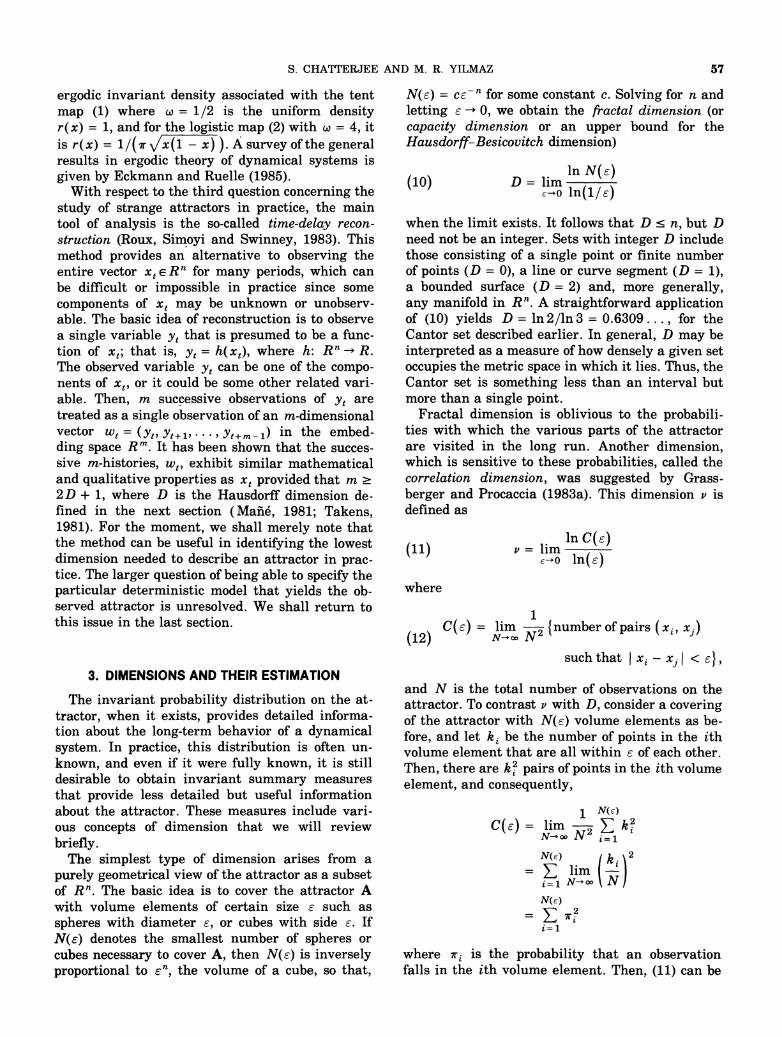
Another approach to chaos is through the study of fractals. Fractals are sets that exhibit ,self- similarity at all levels of magnification, and they may have noninteger dimension that is typical of chaotic attractors. Roughly speaking, self-similarity means that a set remains qualitatively similar in its spatial characteristics under contraction or magnification (more precise definitions can be found in Mandelbrot, 1982, pages 349-350). Transforma- tions such as rotation and displacement retain exact self-similarity, but fractals may exhibit less strict forms of self-similarity obtained via bounded deformations. Mandelbrot (1967, 1977, 1982) first introduced and then popularized the notion of fractals through his beautiful pictures of the Mandel-brot set (Figure 3), which is the iterative map of Z,,, = 2; + C in the complex plane, where C = a + ib is a complex number and Z0 = 0. Hofstadter (1981), Barnsley (1988), Barnsley et al. (1988), Pietgen and Richter (1988), Falconer (1990), among others, give lucid introductions to the mathematics of fractals along, with some beautiful pictures of well-known fractals and their families. Another rich source of computer graphics for iterates of maps and other complex algorithms is Pickover (1990).

The Mandelbrot set is obtained for points that do not go to infinity ( in the extended complex plane) for n + 03. These points form the large cardioid in Figure 3 and many smaller cardioids, such as the one on the right and others that are even smaller, all of which az'e connected with thin lines. The boundary, which is also known as a Julia set, dis-

9. FIG.3. The Mandelbrot set.

plays extremely complicated shapes that look similar at all levels of magnification. The Mandelbrot set is associated with the entire family of iterative maps, resulting from fixing Zo = 0 and varying C, whereas a Julia set is obtained from a single iterative map with fixed C, and an initial point near 0. If the mapping is exponential given by Z,,, =

hexp(Z,), where X is complex, the resulting Julia set is not the boundary of a cardioid but a beautiful sea-horse shape. Gaston Julia and Pierre Fatou, sometimes called the fathers of complex analysis, were the first to study these phenomena, and the iteration of complex exponentials has led to a new field of complex (in the sense of complex numbers) dynamics. In the domain of real numbers, perhaps the best-known fractal is the Cantor set that is obtained by removing the middle third of the real interval [O, 11, then removing the middle thirds of the remaining intervals and so on. The relationship between fractals (Mandelbrot set, Julia set, Cantor set, etc.) and dynamical systems is not well established, but a fractal is often obtained as the asymptotic remnant, or the attractor, of a chaotic dynamical system.

The simplest (first-order) geometric property of a fractal is usually measured by its fractal dimension, also called the capacity dimension (to be discussed in the next section). Higher order geometrical properties of fractals include lacunarity and nonuniformity, which are related to the existence of holes and other irregularities in fractals. Thus, fractals appear in two distinct ways: a de- scriptive tool for studying irregular sets and forms, or a mathematical deduction, resulting from an underlying chaotic dynamic system.

We have organized the paper as follows: in the next section, the theoretical background is re-viewed, including the know^ results concerning the conditions under which chaos arises, relevance of ergodic theory and the reconstruction of attractors. Section 3 reviews various concepts of dimension of an attractor and their estimation in practice. Appli- cation of these ideas in various fields is reviewed in Section 4. The last section includes a discussion and conclusions.

2. BACKGROUND

A complete description of a dynamical system involves, at a minimum, the ability to describe the system status at an instant of time as well as its behavior over any chosen time interval. In the study of physical systems, it has become customary to undertake this pursuit in terms of the phase space of a system, such that points in this space represent instantaneous descriptions of system

54 CHAOS

status at different points in time. Gibbs and Ein- stein introduced the- concept of phase space into physics to account for the fact that it is not possible to "know" the initial states of systems formed by a large number of particles.

To illustrate, imagine a system consisting of a single particle that is in motion in the usual three- dimensional space. An instantaneous description of the system requires three coordinates showin'g the position of the particle and three additional mo- mentum coordinates showing the rates of change in position coordinates. The phase space of this one-particle system is therefore six-dimensional. A system with k particles in motion will have 6k dimensional phase space. It is a fundamental result in classical quantum mechanics that the behavior of a dynamical system can be described by a Hamil- tonian function that depends on the coordinates of the phase space and possibly on time. All systems described by a time-independent Hamiltonian are conservative where there is no net loss of energy, and the volume is incompressible by the Liouville theorem. In dissipative systems, energy and volume must necessarily decrease with time (Nicholis and Prigogine, 1989).

Instead of describing system behavior in terms of a function on the phase space, it is customary to use an evolutionary model relating the position coordinates to the rates of change in these coordinates. In continuous time, a simple evolution model may look like

where i shows the instantaneous rate of change in position x(t) at time t, and w denotes fixed parameters such as the intensity of the force driving the system. A similar equation in discrete time would be

where T is some specified increment of time. If x(t) or xt is n-dimensional, it is customary to refer to (3) or (4) as an n-dimensional model, although the phase space has dimension 2n. Clearly, (3) and (4) are the deterministic counterparts of stochastic Markov processes that specify the probability of transition from one point to another rather than the points themselves. For example, (4) can be regarded as a special Markov process with the transition probability density function P( xt+, 1 x,) = 6(xt+, - fw(xt)) where 6(.) is the Dirac delta function.

It turns out that there is no essential difference between the continuous and discrete-time models of dynamical systems, as long as we wish to study the

system's long-term behavior. This is due to the idea of PoincarQ that the system can be studied in terms of a cross-section of the phase space. Instead of looking at the trajectory described by (3), which requires the solution of differential equations, PoincarQ suggested that we can look at the points at which the trajectory crosses the hyperplane defining the cross-section. Essential characteristics of the description of motion in the phase space (invertibility, differentiability, etc.) are also re-flected on the relationship of successive points on the PoincarQ section. For this reason, the remain- der of this discussion will be in terms of discrete time, with T = 1 for simplicity. Without loss of generality in practice, we shall envision xt as a vector in the n-dimensional Euclidean space R ", and f, is a function from Rn into Rn.

If the function f, is specified, including the parameters w, and if x, is observed at some initial time, say to = 0, then we have

Consideration of limiting behavior of fi(xo) for all possible initial points gives rise to the concept of an attractor. Before the discussion of attractors, however, we shall first note that evolution models that are more complex than (4) can be easily envisioned. For example, consider the second-order model,

which can also be written as

Conceptually, (7) can be thought of as a transformation G, from R ~ "into R2n, and one may think that the increase in complexity is nothing more than an increase in dimensionality. This would be deceiving, since the initial time to can no longer be arbitrarily set to zero and xto can no longer specify the initial state. Clearly, such higher order models are capable of describing even more complicated dynamics, and they are correspondingly more difficult to investigate. At the present time, very little is known about the general properties of these more complex models if f, is nonlinear. We should note that the idea of using a multivariate state space representation of a time series is a common method of analysis, as, for example, in building econometric models with tools such as Kalman fil- tering (Aoki, 1987).


A variation of the model in (6) is

where xt-, has been replaced by t. This model is called nonautonomous as opposed to (4), where f, is time-independent and thus autonomous. Similar to (6) and (7), a nonautonomous system can be converted to an autonomous system by augmenting the state vector with an additional component for time. The results pertaining to the asymptotic behavior of autonomous systems would remain valid if f, is periodic in time, that is, f,(x, t) = f,(x, t + T) for some fixed T. If this is not the case, then the asymptotic behavior may be unbounded and most results for the autonomous case do not apply.

Turning now to autonomous evolution, let us imagine that, initially, the possible states of the system constitute some subset U of R n having positive volume (Lebesgue measure). If the system is dissipative, the volume must be compressed due to loss of energy, and U converges asymptotically to a compact set A. More precisely, A is called an attracting set with fundamental neighborhood U if f:(A) = A for any t, and for every open set V 1A we have f;(U) c V as if t is large enough. The union of the inverse iinages (f;)-'(U) for all t is called the basin of attraction of A. Every trajectory starting at a point in the basin of attraction enters a neighborhood of the attracting set A as t + a.Frequently, the attracting set is also called the attractor, as we shall do here, although it is possible to subtly distinguish between the two terms. More precisely, attractors are smaller subsets of attracting sets consisting of the points around which trajectories accumulate. In any case, due to loss of energy, the volume of A becomes zero but this does not mean that it contains a single stable point. There are many subsets of R n having zero volume, yet they include uncountably many points. In the usual three-dimensional space, for example, any two-dimensional surface has zero volume. Thus, the attractor resulting from long-term behavior of dissipative systems includes a number of interesting 'possibilities that can be classified into one of four categories:

1. Single stable point. 2. Periodic attractor with a fixed period. 3. Quasi-periodic attractor (superimposition of

periodic attractors with different periods). 4. Aperiodic (chaotic) attractor.

In the phase space, the first three types of attractors have shapes with the qualitative characteristics of a point, circle and torus, respectively. An aperiodic (chaotic) attractor does not have one of

these classical shapes and cannot be obtained from them by bounded deformations or diffeomorphisms (invertible and continuously differentiable transformations). For this reason, it is called a strange attractor, a term coined by Ruelle and Takens (1971).

Geometrically, the creation of a chaotic attractor in dissipative systems can be explained as follows: imagine that we begin with a small sphere initially. The sphere may evolve into an ellipsoid after a small enough increment of time. Although the volume of the ellipsoid must be smaller than that of the sphere, the longer principal axis of the ellipsoid can actually be larger than the diameter of the sphere. This means the evolution involves compression in certain directions and stretching in others. For the motion to remain bounded, stretching in a given direction cannot continue forever, and it would have to be accompanied by folding also. If this compression-stretching-folding pattern contin- ues, trajectories that are initially close can diverge rapidly as time goes on. This situation is called sensitive dependence on initial conditions. As we shall investigate in the next section, compression or stretching in the various directions are indicated by the so-called Lyapunov exponents of the system.

Classical Fourier analysis of a periodic attractor would show a power spectrum with a single large spike at a fundamental frequency and evenly spaced low-amplitude harmonics. A quasi-periodic attractor would have several fundamental frequencies and their lower harmonics. A chaotic attractor would have a continuous power spectrum with no obvious spikes or whose component frequencies are smeared out. Building a linear time series model in this case would require infinite dimensions, but a nonlinear model may have a low-dimensional attractor in the phase space. In this sense, nonlinear models are more parsimonious than linear models in describing chaotic behavior. Being able to describe data with parsimonious models hold great attraction for statisticians. We discuss this aspect a little further in the concluding section of this article.

The fact that nonlinear models are capable of generating or describing chaotic behavior leads to several important questions. These questions are compounded by the fact that the same general model can have all four types of attractors depending on the parameter values and initial conditions, as in the logistic model (2). Among the many relevant questions, the following seem to be fundamental in theory as well as practice:

1. What are the- general properties of f, that lead to a chaotic attractor, and what set of

56 CHAOS

parameter values and initial conditions produce these properties?

2. What are the characteristics of chaotic attractors and can they be quantified?

3. Can we observe attractors in practice, and how can we identify the deterministic models that generated them?

4. How can we determine if a deterministic or a probabilistic model would better represent a given process, especially with limited or noisy data?

Only partial answers, and some of them only in specific cases, are available to these questions. They continue to give impetus for a high level of re-search activity in nonlinear systems. We shall survey the currently available results, postponing the last question until the next section.

In the context of one-dimensional models with f, defined on a real interval, some answers to the first two questions were given by Li and Yorke (1975). Their result, which is a special case of an earlier result due to Sarkovskii (1964), says that if f, is continuous and has a periodic point of period 3, then there is a periodic point with any other period k = 1,2, . . . . This implies a chaotic trajectory with arbitrarily large period k. Li and Yorke also showed that there is an uncountable set of such initial points that are ultimately chaotic. It was later asserted (Jakobson, 1981) that, in the logistic model (2), the set of values of the parameter w that yield a chaotic attractor has positive measure (although it may not contain complete intervals). In the tent model (I), almost all initial points (except for a set of points of measure zero) have chaotic trajectories for any value of w between 0 and 1.

With respect to the second question, Li and Yorke showed that, if f, is unimodal, twice continuously differentiable everywhere except at one point, and the absolute value of its slope is greater than 1 everywhere (except at one point), then the limiting behavior of almost all initial points can be described by a time-independent prbbability density function called the invariant density. The probability that the trajectory of an initial point falls in a given interval is found by integrating the invariant density over the given interval.

This result is a special case of ergodic theory that is concerned with measure preserving transformations of general measure spaces (e.g., Billingsley, 1965; Walters, 1982). We shall only summarize the basic results here. In the present context, let p be a probability measure on R n. The function f: Rn -+

Rn is called measure preserving if p(f-'(B)) = p(B) for any subset B c Rn, and p is called an invariant probability measure. This measure is

called ergodic (or indecomposable or metrically transitive) if f -I( B) = B implies p( B) = 0 or p( B) = 1for any B cRn. Here, f - I ( B) is the subset of all points that are transformed onto B by the function f .

If f is a continuous contractive transformation on Rn, then the volume (Lebesgue measure) of any compact subset of Rn is compressed under f. Also, there is a compact subset A c Rn such that f(A) = A. Under repeated applications of f, the entire domain of f converges to A, which is the universal attractor. It is always possible to find an ergodic invariant probability measure p with p(A) = p( f-'(A)) = 1,Given such a measure, we can describe the probabilities with which various parts of the attractor are visited in the long run. In an ergodic system, every state of positive p-measure can be visited, given a sufficiently long time, although the recurrence times may be large. Histori- cally, the fundamental assumption that has linked dynamics and statistical mechanics is the assumption of ergodicity .

The main result in ergodic theory states that if f is measure preserving, p is ergodic, and g: Rn+ R is any integrable function, then

for almost all x E Rn. The "time average" on the left side of (9) is thus equal almost everywhere to the "space average" on the right, where p provides the weights used in the average. This powerful result has many important consequences in statistics, including the laws of large numbers. For example, if E is a subset of the attractor A and g is the characteristic (indicator) function of E , then (9) shows that the probability of E is the limit of the relative frequency that the trajectory f i(x) visits E. If g maps a vector in Rn to one of its components, then the mean of the component is given on the right of (9) as the limit of the time series mean for that component.

Ergodic theory allows the consideration of the long-term behavior of a system without worrying about the transient behavior. On the other hand, establishment of the ergodic property or the determination of an invariant measure associated with a given transformation f are difficult tasks in general. The former task requires the verification of certain "mixing" properties of f which imply ergodicity, and the latter involves the solution of integral equations. Most of the available results pertain to measure-preserving functions on real intervals and few generalizations to higher dimensional spaces are available. For example, an


ergodic invariant density associated with the tent map (1) where w = 112 is the uniform density r(x) = 1, and for the logistic map (2) with w = 4, it is r (x) = 1/ (n J-). A survey of the general results in ergodic theory of dynamical systems is given by Eckmann and Ruelle (1985).

With respect to the third question concerning the study of strange attractors in practice, the main tool of analysis is the so-called time-delay reconstruction (Roux, Simoyi and Swinney, 1983). This method provides an alternative to observing the entire vector x, ER n for many periods, which can be difficult or impossible in practice since some components of x, may be unknown or unobserv- able. The basic idea of reconstruction is to observe a single variable y, that is presumed to be a function of x,; that is, y, = h(x,), where h: Rn + R. The observed variable y, can be one of the components of x,, or it could be some other related variable. Then, m successive observations of y, are treated as a single observation of an m-dimensional vector w, = ( y,, y,, ,, . . . , y,+,- ,) in the embed-ding space Rm. It has been shown that the successive m-histories, w,, exhibit similar mathematical and qualitative properties as x, provided that m 2 2 D + 1, where D is the Hausdorff dimension defined in the next section (Mafib, 1981; Takens, 1981). For the moment, we shall merely note that the method can be useful in identifying the lowest dimension needed to describe an attractor in practice. The larger question of being able to specify the particular deterministic model that yields the observed attractor is unresolved. We shall return to this issue in the last section.

3. DIMENSIONS AND THEIR ESTIMATION

The invariant probability distribution on the attractor, when it exists, provides detailed information about the long-term behavior of a dynamical system. In practice, this distribution is often unknown, and even if it were fully known, it is still desirable to obtain invariant summary measures that provide less detailed but useful information about the attractor. These measures include various concepts of dimension that we will review briefly.

The simplest type of dimension arises from a purely geometrical view of the attractor as a subset of Rn. The basic idea is to cover the attractor A with volume elements of certain size E such as spheres with diameter E, or cubes with side E. If N ( E ) denotes the smallest number of spheres or cubes necessary to cover A, then N(E) is inversely proportional to E ~ , the volume of a cube, so that,

N(E) = C E - ~for some constant c. Solving for n and letting E 4 0, we obtain the fractal dimension (or capacity dimension or an upper bound for the Hausdorff- Besicovitch dimension)

In N(E) D = lim

E+O ln(l/E)

when the limit exists. I t follows that D In, but D need not be an integer. Sets with integer D include those consisting of a single point or finite number of points (D = 0), a line or curve segment (D = I), a bounded surface (D = 2) and, more generally, any manifold in Rn. A straightforward application of (10) yields D = ln 2/ln 3 = 0.6309 . . . , for the Cantor set described earlier. In general, D may be interpreted as a measure of how densely a given set occupies the metric space in which it lies. Thus, the Cantor set is something less than an interval but more than a single point.

Fractal dimension is oblivious to the probabilities with which the various parts of the attractor are visited in the long run. Another dimension, which is sensitive to these probabilities, called the correlation dimension, was suggested by Grass-berger and Procaccia (1983a). This dimension v is defined as

where

C(E)= lim 4{number of pairs ( x i , xi) (12) N+m N

such that 1 xi - xj I < E},

and N is the total number of observations on the attractor. To contrast v with D, consider a covering of the attractor with N(E) volume elements as before, and let k, be the number of points in the ith volume element that are all within E of each other. Then, there are k: pairs of points in the ith volume element, and consequently,

C(E)= lim -I C k:

N+oo N 2 i = l

where ni is the probability that an observation falls in the ith volume element. Then, (11) can be

58 CHAOS

written as

- In C 24'~ v = lim

E+O In(&)

where the numerator is essentially what is known as the order-2 Renyi entropy. The version of C(E)in terms of probabilities has been used in other con- texts also, such as the construction of a surprise index in decision theory (see, e.g., Good, 1952).

A third type of dimension which, like v , takes the probability over the attractor into account is the Balatoni-Renyi information dimension

In S ( E ) a = lim

E+O l n ( l / ~ )

where the numerator is the Kolmogorov-Sinai entropy

Grassberger and Procaccia (1983b) showed that v s a s D. All three dimensions are invariant under invertible differentiable transformations on Rn.

Still another dimension, called the Lyapunov dimension, is defined in terms of the Lyapunov exponents of the process. Lyapunov exponents gen- eralize the concept of instantaneous rate of change with respect to the initial state, in that they indi- cate the average rates of divergence (expansion) or convergence (contraction) of initially close trajectories on the attractor. With f,: Rn+ Rn, there are n Lyapunov exponents A, 2 X,2 . . 2 An, so that Xi < 0 indicates an average rate of contraction and Xi > 0 indicates repeated expansion and folding in a particular dire~tion (the direction of the corre-sponding eigenvector of the Jacobian matrix of partical derivatives). Their existence in ergodic dynamical systems is due to the multiplicative er-godic theorem (Oseledec, 1968). Any dissipative system with n > 1must have at least one negative exponent, and the sum of all exponents must be negative, indicating an overall contraction. A system with a chaotic attractor must have at least one positive Lyapunov exponent.

Lyapunov exponents can be visualized geometrically in the following way: imagine that the initial state of the system can lie in an infinitesimal n-dimensional sphere with diameter Po.After N periods, assume that the sphere becomes an ellipsoid, with PiNbeing the length of its ith largest principal axis. Then, piN/POis the overall proportional change in the length of the principal axis, and ( ~ / N ) ~ ~ ( P , ~ / P O )is a measure of the average rate

of change. The limit of this average as N -+ cn is the ith Lyapunov exponent. Mathematically, PiN/POis the determinant of the Jacobian matrix of partial derivatives evaluated at the initial point xo.

Suppose the Lyapunov exponents are placed in descending order, and let j be the largest integer such that h, + & + . . +Xj 2 0. The Lyapunov dimension is then defined as

It was originally conjectured that DL = D (Kaplan and Yorke, 1979), for which counter examples were found (see, e.g., Grassberger and Procaccia, 1983b). The relationship between DL and other dimensions has not yet been clearly established, but a more restrictive form of the Kaplan-Yorke conjecture was proved by Ledrappier and Young (1988).

For systems whose evolution equations are given, calculation of all Lyapunov exponents is possible, although it is computationally burdensome. With experimental data, however, there are no known methods to estimate all exponents. The best known of the existing methods (Wolf, Swift, Swinney and Vastano, 1985) is capable of estimating only the positive exponents, but more recent progress is Nychka, McCaffrey, Ellner and Gallant (1990), and Brown, Bryant and Aberband (1991). Currently, there are no widely available means to estimate DL from experimental data.

The algorithm of Wolf, Swift, Swinney and Vas- tan0 operates on the basis of normalization, which is the physicist way of obtaining a finite-sized picture of an infinitesimal geometry. Any property of the original that depends only on the infinitesimal geometry can be read off from the finite geometry of the normalized object. Mathematically, this normalization is carried out by the Gram-Schmidt orthogonalization scheme.

Estimation of other dimensions has been somewhat more fruitful, although significant problems remain with all available methods. The problems arise from the basic facts that dimensions are defined as limits whose existence must be ascertained and estimates obtained on the basis of a finite set of data. The fact that data may include noise com- plicates these problems. Thus, the problem boils down to whether or not the system under study can be observed long enough and with sufficient preci- sion to satisfactorily address these issues.

Available methods for dimension estimation can be classified into two groups, which may be called fixed-size and fixed-mass methods. In the fixed-size (box-counting) approach, the space is divided into a


grid of boxes of fixed side E. Then, we can count the number N(E) of nonempty boxes, the number ki of points in the ith box, the fraction ki / N of data points in each box or the number of pairs of points that are within E of each other. By varying E, and fitting a line to the plot of In N(E) versus l n ( l / ~ ) , the estimate of D is obtained as the slope of the fitted line. Estimates of v and a are obtained simi- larly as the slopes of CN(&) versus In E, and In SN(&) versus ln(l/ E), respectively. Here, C N ( ~ ) and SN(&) are the respective sample counterparts of C(E) and S(E) with N observations.

In the fixed-mass (nearest neighbor) approach, one fixes the number k of points to be contained in each neighborhood and determines the diameter of the neighborhood accordingly. Generally speaking, this approach is computationally more efficient than the fixed-size approach. Discussion of the various algorithms can be found in Greenside, Wolf, Swift and Pignatoaro (1982), Meyer-Kress (1986), Somor- jai (1986), Kostelich and Swinney (1987), Dubuc et al. (1989), and Taylor and Taylor (1991). For the estimation of the correlation dimension, recent en- hancements using singular value decomposition have been proposed by Albano et al. (1988) and Broomhead and Jones (1989).

One of the important questions in dimension estimation involves the sampling distributions of the estimates. Presently, few general results are available concerning this question. Maximum-likelihood estimation of the correlation dimension has been discussed by Takens (1984). Denker and Keller (1986) showed that, under quite general conditions, CN(&) converges in probability C(E), SO that the slope of the linear regression of CN(E) on E yields a consistent and asymptotically unbiased estimate of v. Cutler and Dawson (1989) show that if the attractor constitutes a smooth D-dimensional subset of Rn (D an integer), then the local (pointwise) dimension at any given point is equal to D, with probability 1.Unfortunately, their results have not been extended to attractors with noninteger D. It 'seems that distribution of dimension estimates will be an active research topic for some time to come.

Before concluding the discussion of dimension, let us return to the time-delay reconstruction of attractors from experimental data. As noted previously, if x, = f(x,-,) and y, = h(x,) where f: Rn- t R and h: Rn -t R, then the attractor of x, can be reconstructed from m-histories of y,. If m r 2 D + 1, where D is the fractal dimension of the attractor of x,, then the reconstructed attractor of the m-histories shares many of the qualitative features of the original, and the correlation dimension of the reconstruction is equal to that of the original attractor. When m is unknown, as is usually the

case, it can be estimated in the following ad hoc fashion: start with m = 1and obtain the estimate i of the correlation dimension of the reconstructed attractor. Next, increment m by 1 and repeat the calculation. Continue until i does not change sig- nificantly. The final i is the estimate of the correlation dimension of the attractor and, the lowest m yielding this estimate is the dimension of the reconstruction space.

It has been suggested that reconstruction provides a means for deciding whether a chaotic uni- variate time series { y,) has been generated by a deterministic or random process (Takens, 1985; Brock, 1986). The time series is said to admit a smooth deterministic explanation if there exist continuously differentiable functions h and f, with y, = h(x,) and x, = f(xt- ,). Given that { y,} admits a smooth deterministic explanation, then the correlation dimension must be low (independent of m for m r 2D + I), and the largest Lyapunov exponent must be positive. In addition, Brock (1986) claims that if a linear autoregressive model of order L is fitted to { y,}, then the residuals from this model should have the same dimension and Lyapunov exponent as { y,}. Because these assertions are necessary but not sufficient for the existence of a deterministic explanation, their usefulness is severely limited in practice. Sufficient conditions for a low-dimensional deterministic explanation have not yet been discovered.

4. APPLICATIONS

We discuss various applications of chaos, fractals and related ideas in different disciplines that have been reported in the literature. Our emphasis will be on applications other than in the field of physics where there are already many good references (e.g., Bergh, Pomeau and Vidal, 1984).

4.1 Chaos and Fractals in Mathematics

The idea of defining an outer measure to extend the notion of length of an interval is of relatively recent origin in mathematics. Measures of sizes of sets originated with Bore1 (1895) and continued by Lebesgue (1904) as an underlying concept in the construction of an integral. Carathhodory (1914) introduced the more general concept of outer measures that is the notion of linear measure in n-dimensional Euclidean space. Hausdorff (1919) extended CarathBodory's measure to nonintegral dimensions. This was shown by illustrating the Hausdorff dimension of the Cantor set to be ln 2/ln 3 = 0.6309. [This measure generalizes to In 2/ln(l/ k) if the portion removed from the middle of a unit interval is (1 - 2 k).]

60 CHAOS

Sets of fractional dimension also occur in diverse branches of pure mathematics, such as the theory of numbers and nonlinear differential equations. Motivated by the theory of Brownian motion, measures of sets of curves were developed by Weiner in the 1920s that found widespread application in the theory of control and communication. An up-to-date geometric theory of sets with fractional dimension is given in Falconer (1985, 1990). Good (1941) gives an early example of an application in number theory. Further technical discussions of fractals, self-similarity, dimension and dynamics of fractal recurrent states can be found in Hutchinson (1981) and Bedford (1986). Investigations into asymptotic periodic behavior, transition to chaos and other dynamical consequences for ordinary differential equations are reported by Gardini, Lupini, Mam- mana and Messia (1987), Nusse (1987) and Wiggins (1988).

Use of functional iterates in the theory of branch- ing processes goes back at least to the work of Hawkins and Ulam (1944) and Good (1965). Thus, let f(x) be the Laplace generating function of a sequence of probabilities { p,, p,, p,, . . . }, then the probability that an individual has k male descen- dants in the nth generation is given by the coeffi- cient of xk in f "(x) where f "(x) = f( f "-'(x)). Neutron multiplication in fission and fusion de- vices are other practical applications of functional iterations.

A related area of great interest is the theory of cellular automata in which a discrete dynamical system evolves in a space of uniform grid of cells. In contrast to continuous dynamical systems modeled via differential equations or iterates of maps, theory of cellular automata specifies the system's behavior in terms of a set of local values that apply to all cells at each discrete increments of time. Study of cellular automata is a separate area in itself, with many application areas such as parallel computing, image processing and pattern recognition. Toffoli and Margolus (1987) and Preston and Duff (1984) are good introductions'to this area.

From the viewpoint of our discussion, theory of cellular automata is relevant for at least two rea- sons: first, it provides a methodology for approxi- mating continuous systems and, second, it affords an alternative model for complex system behavior in terms of known initial conditions and simple rules of evolution. Thus, cellular automata are capable of arbitrarily complex behavior with special properties of self-replication, efficient energy trans- duction and so on (Wolfram, 1984, 1986; Nicolis and Prigogine, 1989). Such systems are examples of self-organization phenomena, and the field of syner- getic~ is an outgrowth of study of such systems

(Haken, 1978). For other applications of cellular automata and a good account of the theory of functional iterations and nonlinear deterministic models, see Stein (1989).

Cellular automaton models involve a great many variables, one for each cell, as opposed to models with differential equations or iterations of maps that require very few variables. On the other hand, many of the ideas and methods associated with fractals and dynamical systems, such as concepts of dimension and entropy, are applicable in the context of cellular automata. Another notion that is especially important in the latter context is algorithmic complexity.

Use of notions of algorithmic complexity and their measures were first proposed by Kolmogorov (1965, 1983) and later developed by Chaitin (1987). Algo- rithmic complexity of a string of zeroes and ones is given by the number of bits of the shortest computer program that can generate this string. Such measures of complexity are useful for describing cellular automata and pattern formation. Rissanen (1986) has used this idea of algorithmic complexity for order determination in statistical models. The notion of complexity in a more general context was discussed in several papers by Good and summa- rized in Good (1977). Descriptions and characterization of complexity in spatiotemporal patterns for high-dimensional nonlinear systems is discussed by Kasper and Schuster (1987).

4.2 Chaos in Physiology, Biology and Epidemiology

To begin with, fractal-like structures are found in networks of blood vessels, nerves and ducts within much of the human body and other living things. Work on distinguishing between healthy and un- healthy systems in the body is currently an interesting and challenging case in dynamical systems. For example, does a healthy heart produce physiological data with its fractal dimension and other characteristics that are different from an un-healthy heart? It is known, for example, that normally chaotic oscillations of the densities of the red and white blood cells become periodic in some anemias and leukemias. Such questions can be carefully investigated in laboratory settings. Physiological variables generated from electro-cardiogram, immunoreactive insulin and electro- encephalogram are great data sources, where the presence of attractors of varying characteristics may be useful in indicating a state of general health, onset of disease or measuring its progress. This would complement the existing mathematical models of physiology, such as the "integrate and the fire model," in which activity rises (integration) to


a threshold leading to an event (firing). Neuronal activity is thought to. be a good example of this.

Many physiological rhythms are generated by a single cell or electrically coupled isopotential cells that are capable of generating oscillating activity. From both theoretical and experimental viewpoints in neurobiology, many pacemakers capable of dis- playing regular periodic oscillations may also have irregular dynamics. Such models are known as Hodgkin and Huxley (1952) models. A detailed analysis of this viewpoint and its relationship to chaos can be found in Rapp (1979, 1981) and Glass and Mackay (1988). In the absence of chaos, either very dull pacemaker activity or highly explosive global neural firing patterns might emerge. Chaos would serve to maintain the functional independence of different parts of the nervous system and thereby make it more adaptable. For applications of chaos in neurophysiology and neurobiology, see Baird (1985), Clarke, Rafelski and Winston (1985), Schmajuk and Moore (1985) and Skarda and Free- man (1987).

The use of chaos as supporting evidence of the theory of punctuated evolution has been proposed by Conrad (1983, 1988). Small events (mutations) undergo averaging, thereby cancelling any net effects; but once in a while a single event (mutation) becomes all important and directs the path of evolution in new directions and patterns that are then preserved and built on afresh. The final position at any point in time might as well have been arrived at by both chance and necessity (Monod, 1973). Mechanisms of adaptability that involve diversity generation in which'chaotic mechanisms play a key role are being studied by scholars of evolutionary biology. Conrad (1988) provides three useful functions for chaos: (i) search (diversity generation), which can be both genetic and behavioral; (ii) defense (diversity preservation), which can be im-munological, behavioral or populational; and (iii) prevention of entrainment, that is, being locked into a certain phase of existence.

Population biology is an area' where the importance of nonlinear dynamics was felt even before the work of Lorenz. There have been many models of population biology that use simple systems of differential equations to describe growth behavior of living species in their natural ecology. An up-to- date review of these models is provided by May (1987). Moran (1950), in a,n entomological context, discovered stable points, limit cycles and events that we call chaos today. For example, a second-order version of the logistic model (2), called the Verhulst process is given by

x ~ + ~= ux t ( l - xt-,) for 0 < xt < 1.

This relatively simple model is a special case of more general models of predator-prey relation-ships. It has an extremely complicated attractor for a range of w values, such that there are some initial values that lead to extinction and other values lead to cycles or chaotic fluctuations. Tor- roidal flow (flow on a torus), when the motion is quasi-periodic, is a model for a predator-prey relationship in a seasonal environment (Inoue and Kamifukumoto, 1984), and strange attractors give rise to chaos in a one-predator, two-species environment (Shibata and Saito, 1984). The dynamical properties of models in population biology is reviewed in Gauss (1964), Kloeden and Mees (1985) and May (1973, 1986, 1987). The combination of population biology with population genetics leads to a deep study of nonlinear phenomena involving genetic polymorphisms that may vary cyclically or chaotically, as discussed by May (1987).

The discovery of mathematical chaos has naturally led biologists in search of observable chaos in nature. However, observed data are polluted with environmental (statistical) noise that makes their detection difficult. Thus, finding examples of time series data that clearly show period doubling, inter- mittency, transition to chaos and other behavior of nonlinear systems is a challenge facing the current generation of population biologists.

In epidemiology, the study of motions of populations, including human disease, is also of interest in models of chaos. If the fluctuations in epidemics are due to deterministic chaos, then they have more structure than previously believed. Under- standing this extra structure may help predict such things as the proportion of diseased population and the effects of a vaccination program. The key to such exploration is matching the complex behavior with a specific system of differential or difference equations. Schaffer and Kot (1985) and Schaffer, Ellner and Kot (1986) have concluded that measles, mumps and rubella data from Copenhagen behave chaotically, whereas data on chicken pox show regular cycles; whereas for still other data sets, the evidence of the existence of an attractor is inconclusive.

4.3 Chaos in Economics

The theory of chaos and dynamical systems has been applied in economics from both a theoretical and empirical perspective. In the theoretical perspective, existence and study of multiple equilibria based on positive feedback is due to Arthur, Yu and Yu (1987) and Arthur (1990). The classical theory of Marshall and Adam Smith relies on interaction or negative feedback of demand and supply that gives rise to a unique equilibrium value. On the

AOS

other hand, economics based on positive feedback allow multiple equilibria, and allows chance and chaos to play a role in the final outcome. These models of economic activity based on positive feedbacks are based on urn models of Ehrenfest and Polya (Kac, 1959) and nonlinear generalizations of them by Hill, Lane and Suddereth (1980) and Arthur, Ermoliev and Kaniovski (1983). An up-to- date account of applications of nonlinear science in economic theory is given in Anderson, Arrow and Pines (1988).

The empirical economists are interested in test- ing hypotheses on the model generating the path of the economy. Specifically, Brock and Mallaris (1989), Scheinkman and LeBaron (1989) and others are interested in hypotheses of the following kind: is the GNP data generated by a nonlinear deterministic model? Numerical investigations have been conducted by Brock and others on national income and stock market data with inconclusive results. Whereas this type of research may be interesting, it is difficult to find useful and meaningful directions for advancement from this strategy with regard to either understanding of economic forces or improved methods of forecasting. Critics of using deterministic models for economic time series include Sims (1984) and Granger (1987).

4.4 The Role of Chaos in Philosophy and Logic

The role that chaos may play in any philosophical system is discussed by Conrad (1988), Penrose (1989) and Rossler (1986). The discovery of chaos provides evidence that the question of whether a given random-appearing behavior is probabilistic or deterministic in reality may be undecidable, since both types of models may describe the observations equally well. Undecidability of determinism versus indeterminism was asserted earlier by Good (1950, page 15) and others. Some interesting issues of computability of fractals on universal computers are of interest to both physicists and logicians. Penrose (1989) gives the Mandelbrot set as an example of a recursively enumerable set that is not recursive. It appears that there is no known algorithm to decide whether a point on the boundary of the cardioid remains bounded under the map Z+

Z2+ C. Thus, strictly speaking, the boundary of the Mandelbrot set is not computable and the visi- ble Mandelbrot set is only an approximation. Inter- estingly enough, it is at the boundary of this set where intricate structures are born and where (self-similar) fractals grow.

The existence of chaos at the quantum mechanical level (quantum chaos) also appears to be elusive. Classical chaos imply fractal attractors (structures on all scales), but in quantum mechan-

ics structure does not exist on a scale smaller than Planck's constant. Some day quantum mechanics may replace the probabilistic wave function by a deterministic but chaotic one. Berry (1987) gives an up-to-date account of this fascinating theory. Thus, the science of chaos joins a long list of undecidable propositions that includes Godel's undecidable proposition in logic, Heisenberg's uncertainty principle in quantum mechanics and Arrow's im- possibility theorem in economics concerning how to define social rationality (Arrow, 1963).

The current popularity of chaos is also of interest to historians of science and philosophy. We began our essay with quotes from Laplace and Poincar6 depicting the changing views of nature: from total regularity to completely irregular and unpre-dictable behavior of observed nature. This changing view of nature is consistent with modern philosophical doctrines (Cohen, 1987).

4.5 Other Applications

This section describes other applications in various fields. That these applications are grouped to- gether is in no way meant to imply any lesser degree of importance. On the contrary, this group- ing will emphasize the astounding diversity of applications that have already been undertaken.

Barnsley et al. (1988) have written rule-based algorithms that produce realistic-looking images of pine forests, ferns, human faces and many other natural objects. Fractal forgery allows storage of images in a very small amount of space (fractal shorthand) and easier transmission (Barnsley and Sloan, 1988; Brammer, 1989), and this has spurred great advancement in the video image and motion picture industry.

Pickover (1988) studies pattern formation and chaos in networks as a result of propagation of signals through complicated networks. Orbach (1986) uses the self-similarity property of fractals to model percolating networks that describe various physical structures, such as gels, polymers and the transverse force constant of glassy materials. Orbach's work is important because he shows how fractal geometry is not only useful in describing static structural properties, but also in describing the dynamic properties of fractal networks (fractal diffusion).

Goodchild and Mark (1987) summarize the use of fractal geometry in geography that has an earlier origin in Mandelbrot's work (1967). A wide variety of spatial phenomena have been shown to be statis- tically self-similar, which shows scale independence of geographic norm. A fractal dimension provides a means of characterizing the effects of cartographic generalizations and predicting the behavior of


estimates derived from data that is subject to spatial sampling. Fractional Brownian motion (Mandelbrot and Van Ness, 1968; Mandelbrot, 1971; Matalas and Wallis, 1971) provides a method of generating irregular self-similar surfaces that re- semble topography of fractional dimension.

Study of fractals in modeling patterns of erratic occurrence of gaps separating two consecutive cache misses in computer memory is due to Thihbaut (1988). Investigations into characteristics of large telecommunications, computer and other networks using concepts from fractal geometry and graph theory have appeared in the literature. The approach is to study global characteristics of networks, parameterized by a fractal dimension, without resorting to detailed descriptions (Bedro- sian and Jaggard, 1986). Applications of fractal geometry and space-filling curves to combinatorial problems belonging to the NP-complete class and other areas of operations research is due to Platz- man and Bartholdi (1990). NP-complete refers to a class of discrete optimization problems for which no polynomial time algorithm is known to exist (any algorithm that correctly solves an NP-complete problem will require an exponential time).

Applications in geology include study of relationship between ore grade and tonnage through a fractal approach where a high-fractal dimension indicates a strong volumetric concentration of an element (copper, silver, etc.). Such models provide a basis for estimating mineral reserves (Turcotte, 1986).

Study of dynamical systems through interactive computer and expert- systems has been proposed by Abelson et al. (1989), who present automatic preparation, execution and control of numerical experiments to discover and interpret qualitative behavior of dydamical systems. Such programs study ranges of parameters, state variables to be explored, and analyze approximations, divergence characteristics of trajectories and use of minimum spanning trees for clustering of orbits.

Applications to nonphysical problems, such as that: of international security through a simplified procurement model of the Strategic Defense Initia- tive, is due to Saperstein and Meyer-Kress (1989). They use the model to explore the outcomes of various deployment modes and study what they called "crisis instability" through numerical simu- lations.

4.6 Chaos and Fractals in Statistics

Although deterministic models have been used for several decades for generating pseudo random numbers in simulation experiments, the renewed

interest in them is due to their possible use in modeling actual real-world processes that have tra- ditionally been studied through stochastic models. As yet, however, there are no known methods for "fitting" a deterministic model to an actual process. Present state of the art is at the initial stages of studying and cataloging the behavior of various models, and to use expertise and judgment to see if a particular model adequately describes an actual process under investigation.

A potentially important new tool resulting from the theory of chaos is the method of time-delay reconstruction of attractors from time series data. This method can give an idea about the minimum dimension of the underlying process, as well as its long-term behavior. On the other hand, the reconstruction typically requires very long series, and it is sensitive to noise in the data (Ben-Mizrachi, Procaccia and Grassberger, 1984). Noise reduction procedures specifically designed for reconstruction, such as the method of Kostelich and Yorke (1987), are of great interest in this regard. These methods can complement traditional tools, such as factor and discriminant analyses, nonparametric smooth- ing methods and projection pursuit.

A different route to model identification was recently suggested by Chatterjee and Yilmaz (1991). This method does not involve reconstruction, and it does not seek a deterministic model that generates an observed time series. Instead, it focuses on residuals resulting from any given stochastic time series model under consideration, such as ARIMA(p, q), and tries to determine if the residuals appear to fit a white noise process. For the latter task, the estimated fractal dimension of the residuals is com- pared with the fractal dimension of the white noise process.

Another potentially useful tool for the statistician is the idea of fractal interpolation (Barnsley, 1988). Given a finite number of observations, this method generates a complete path interpolating the observations and in a manner consistent with self-similarity. This idea can be useful in handling missing values in the data, and it is illustrated by Chatterjee and Yilmaz (1991). Its usefulness for prediction purposes remains to be investigated.

Another recent modeling tool that seems to have been motivated by fractals and fractal dimension is the notion of fractional differencing in the ARIMA (p, d, q) models, where d is noninteger. This idea can be used to model persistence (long memory) and antipersistence (short memory) behavior. The process (0, d, 0), -112 < d < 112 has been used by Mandelbrot and Van Ness (1968), Mandelbrot (1971) and Matalas and Wallis (1971) for simulat- ing hydrologic data that show long-term memory.

64 CHAOS

An ARIMA(0, d ,0) process x, is defined as

where E~ is a white noise process and B is the backward shift operator. Noting that,

it is easy to see the slowly decaying weights on past observations. Thus, ARIMA(0, d, 0) provides long- term persistence behavior, whereas ARIMA( p,0, q) describes short-run persistence. Granger (1980), Granger and Joyeux (1980), Hosking (1981), Geweke and Porter-Hudak (1983) and Carlin and Dempster (1989) discuss ARIMA(p, d, q) with noninteger d, thus generalizing the procedures of Box and Jenkins (1970). These authors have investigated different properties of fractionally differenced models and estimation procedures, and provided some sampling theory.

5. DISCUSSION AND CONCLUSIONS

The theory of chaos is fascinating if for no other reason than the blurring of the long-held distinc- tion between random and deterministic phenomena. It is potentially capable of "explaining" very complex processes with simple, parsimonious models and essentially without error. This would seem to be sufficient reasan for the statistician to pay attention to the emerging theory and actively par- ticipate in its development. Such participation requires the statistician to be prepared to think in terms of iterations of functions rather than stochastic processes, attractors rather than spectra and embeddings in a phase space rather than time series. In return, the statistician gets a richer set of tools at his or her disposal, although the power and ,limitations of the new tools will ,have to be sorted out.

As we noted throughout, there are many important questions about the new theory that are currently unresolved, and it is likely that some of these issues will never be resolved. The question of choosing between deterministic versus stochastic modeling of a process under study is one such issue, but stochastic modeling presently has a clear advantage because of its rich variety of model-fitting tools. On the other hand, given that we wish to use a deterministic model, it would be imperative to have some means for deciding which specific model to use. Although methods or guidelines for this

purpose are not yet available, we can expect progress in this direction as a larger variety of models are studied.

Another immediate problem in the application of the new theory is the possibility that the observed data includes a random component of environmental noise. In experimental settings, it may be possible to know the sources of noise and minimize it, but this may not be possible when data pertains to real world phenomena. Thus, a basic question is how to recognize the presence of noise and how to separate it from the deterministic effect. In the presence of noise, say E ~ , one could contemplate a model such as

X t + l = f' , ,(~t,.. ., X~-L,~ t )

and if noise is additive, this would become

If E~ is a stochastic process, then the advantage of deterministic modeling over the classical stochastic approach would disappear.

Unlike the deterministic approach, stochastic modeling involves an attempt to separate structure (pattern) in the data from lack of structure (nonpat- tern), and for this reason, it naturally allows for the presence of noise and other random elements. Although deterministic modeling can deal with very small amounts of noise, it provides no means for recognizing its existence in the first place. Contro- versy and research in this area are likely to continue for the foreseeable future.

Present state of the art of dynamical modeling is such that the ability to make general statements about the long-term behavior of a dynamic process requires the assumption that transients have died out and motion has reached the attractor. In experimental settings, it may be possible to wait until this happens. In many real-world processes, on the other hand, we may be perpetually observing transient states due to changes in the environment or even changes in system parameters (bifurcations). More importantly, we do not yet have methods of determining if observed data include such changes or transients.

In summary, then, there are various distinct situations in which we must currently turn to stochastic models, even if a deterministic model is desired. These situations include:

1. Initial conditions are unknown. 2. Process cannot be observed without random

error or noise. 3. Process cannot be observed long enough. 4. Inability to fit a deterministic model even

when situations 1to 3 are not at issue.


Consequently, stochastic models are likely to continue to serve as prototypes for nonlinear deterministic models.

The discovery of chaos in mechanical systems and the subsequent development of mathematical and physical theories of nonequilibrium physics, relationship of physical and algorithmic complexity and mathematical experiments on the computer (ranging from cellular automata to theorems in number theory) may yet prove to be events of great importance. There are those who believe that these developments are of equal import to Einstein's theory of general relativity and Heisenberg's un-certainty principle (Gleick, 1987; Cooper, 1989; Rossler, 1986). Undoubtedly, the quantitative description of chaos is one of the triumphs of nonlinear science. The twenty-first century should see the blossoming of this aspect of nonlinear science, in which statistics and data analysis are likely to play a major role.

ACKNOWLEDGMENTS

We thank Professor I. J. Good for making many comments to improve the readability of the paper. Three anonymous referees, the editor and Hal Stern also provided us with many helpful comments. We also thank James Garahan and Professor Samprit Chatterjee for useful discussions and for providing many references. Professors Cutler and Tsay are also acknowledged.

REFERENCES

ABELSON,K., EISENBERG, M., KATZENELSON, H., HALFANT, J., SACHS, E., SUSSMAN, J., WISDOM, J. and YIP, K. (1989). Intelligence in scientific computing. Comm. ACM 32 546-562.

ALBANO,A. M., MUENCH, J. , SCHWARTS, C., MEES, A. I. and RAPP, P. E. (1988). Singular-value decomposition and the Grassberger-Procaccia algorithm. Phys. Rev. A (3) 38 3017-3025.

ANDERSON, D. (1988). The Econ- P. W., ARROW, K. and ~ E S , omy as an Evolving Complex System. Addison-Wesley, Read- ing, Mass.

AOKI, M. (1987). State Space Modeling of Time Series. Springer, New York.

ARROW, K. J. (1963). Social Choice and Individual Values, 2nd ed. Wiley, New York.

ARTHUR,W. B. (1990). Positive feedbacks in the economy. Scien- tific American 262 92-99.

ARTHUR,W. B., ERMOLIEV, Y. (1983). On Y. and KANIOVSKI, generalized urn schemes of the polya-kind. Cybernetics 19 61-71.

ARTHUR,W. B., Yu, M. E. and YU, M. K. (1987). Path depen- dent processes and the emergence of Marco Structure. Euro- pean J. Oper. Res. 30 294-303.

BAIRD, B. (1985). Nonlinear dynamics of pattern formation and pattern recognition in the rabbit olfactory bulb. Phys. 022 150-175.

BARNSLEY,M. F. (1988). Fractals Everywhere. Academic, Boston.

BARNSLEY,M. F., DEVANEY, R. L., MANDELBROT, B. B., PEITGEN, H. O., SAUPE, D. and Voss, R. F. (1988). The Science of Fractal Images. Springer, New York.

BARNSLEY,M. F. and SLOAN, A. D. (1988). A better way to compress images. Byte 13 215-218.

BARTLETT,M. S. (1990). Chance or chaos? (with discussion). J. Roy. Statist. Soc. Ser. A 52 321-347.

BAUMOL, J. (1989). Chaos: significance, mech- W. and BENHABIB, anism and economic applications. Journal Economic Per- spectives 3 77-105.

BEDFORD,T. (1986). Dimension and dynamics for fractal recurrent ets. J. London Math. Soc. 33 89-100.

BEDROSIAN, D. L. (1986). A fractal-graphS. D. and JAGGARD, approach to large networks. Proc. IEEE 75 966-968.

BEN-MIZRACHI, I. and GRASSBERGER, A., PROCACCIA, P. (1984). Characterization of experimental (noisy) strange attractors. Phys. Rev. A (3) 29 975-977.

BERG$, P., POMEAU, Y. and VIDAL, C. (1984). Order Within Chws. Wiley, New York.

BERLINER,L. M. (1992). Statistics, probability and chaos (with discussion). Statist. Sci. 7 69-121.

BERRY,M. V. (1987). Quantum chaology. In Dynamical Chaos (M. V. Berry, I. C. Percival and N. 0 . Weiss, eds.) 183-197. Princeton Univ. Press.

BILLINGSLEY,P. (1985). Ergodic Theory and Information. Wiley, New York.

BOREL,E. (1895); Sur quelques points de la thkorie des fonctions. Ann. Ecole Norm. 12 9-55.

Box, G. E. P. and JENKINS, G. M. (1970). Time Series Analysis: Forecasting and Control. Holden-Day, San Francisco.

BRAMMER,R. F. (1989). Unified image computing based on fractals and chaos model technique. Optical Engineering 28 726-729.

BROCK,W. A. (1986). Distinguishing random and deterministic systems: abridged version. J . Econom. Theory 40 168-195.

BROCK, W. A. and MALLARIS, A. G. (1989). Differential Equa- tions, Stability and Chws in Dynamic Economics. North- Holland, Amsterdam.

BROOMHEAD,D. S. and JONES, R. (1989). Time-series analysis. Proc. Roy. Soc. London Ser. A 423 103-121.

BROWN,R., BRYANT, H. D. (1991). Computing P. and ABERBAND, the Lyapunov spectrum of a dynamical system from an observed time series. Phys. Rev. D 43 2787-2806.

CARATH~ODORY, das Lineare Mass von Punkt- C. (1914). ~ b e r mengeneine Verallgemeinerung des Langenbegriffs. Nach Ges Wiss, Gijtingen.

CARLIN,J. B. and DEMPSTER, A. P. (1989). Sensitivity analysis of seasonal adjustments: Empirical case studies. J. Amer. Statist. Assoc. 84 6-20.

CHAITIN,G . J . (1987). Algorithmic Information Theory. Cam- bridge Univ. Press.

CHAT~ERJEE, M. R. (1991). Use of the estimated S. and YILMAZ, fractal dimension in model identification for time series. Preprint.

CLARKE,J . W., RAFELSKI, J . and WINSTON, J . V. (1985). Brain without mind: Computer simulation of neural networks with modifiable neuronal interactions. Phys. Rep. 123 215-273.

COHEN,I. B. (1987). Scientific revolutions, revolution in science and a probabilistic revolution 1800-1930. In The Proba- bilistic Revolution (L. Kriiger, L. J. Daston and M. Heidel- berger, eds.) 1 23-44. MIT Press.

COLLET, P. and ECKMANN, J.-P. (1980). Iterated Maps on the Interval as Dynamical Systems. Birkhauser, Boston.

CONRAD,M. (1983). Adaptability. Plenum, New York. CONRAD,M. (1988). What is the use of chaos? In Chws (A. V.

Holden, ed.) 3-14. Princeton Univ. Press.

66 CHAOS

COOPER,N. G. (1989). From Cardinals to Chaos. Cambridge Univ. Press.

CUTLER,C. D. and DAWSOM, D. A. (1989). Estimation of dimensions for spatially distributed data and related limit theorems. J . Multivariate Anal. 28 115-148.

DEGROOT,M. (1986). A conversation with Persi Diaconis. Statist. Sci. 1 319-334.

DENKER,M. and KELLER, G. (1986). Rigorous statistical procedures for data from dynamical systems. J . Statist. Phys. 44 67-93.

DEVANEY,R. (1989). A n Introduction to Chaotic Dynamical Systems, 2nd ed. Addison-Wesley, Reading, Mass.

DUBUC, B., QUINIOU, J . F., ROQUES-CARMES, C. and C., TRICOT, ZUCKER,S. W. (1989). Evaluating the fractal dimension of profiles. Phys. Rev. A (3) 39 1500-1512.

ECKMANN, D. (1985). Ergodic theory of chaos J.-P. and RUELLE, and strange attractors. Rev. Modern Phys. 57 617-656.

FALCONER,K. J . (1985). The Geometry of Fractal Sets. Cam-bridge Univ. Press.

FALCONER,K. J. (1990). Fractal Geometry. Wiley, New York. FEIGENBAUM,M. (1978). Quantitative universality in a class of

non-linear transformations. J. Statist. Phys. 19 25-52. GARDINI,L., LUPINI, R., MAMMANA, C. and MESSIA, M. G. (1987).

Bifurcations and transitions to chaos in the three-dimensional Lotka-Volterra map. SIAM J . Appl. Math. 47 455-482.

GAUSS, G. F. (1964). The Struggle for Existence. Haffner, New York.

GEWEKE,J . and PORTER-HUDAK, S. (1983). The estimation and application of long memory time series models. J . Time Ser. Anal. 4 221-238.

GLASS, L. and MACKAY, M. C. (1988). From Clock to Chaos: The Rhythms of Life. Princeton Univ. Press.

GLEICK,J. (1987). Chaos: Making of a New Science. Viking, New York.

GOOD,I. J . (1941). The fractional dimension theory of continued fractions. Proceedings of the Cambridge Philosophical Soci- ety 37 199-288.

GOOD, I. J . (1950). Probability and the Weighting of Evidence. Charles Griffin, Londcn.

&OD, I. J. (1952). Rational decisions. J . Roy. Statist. Soc. Ser. B 14 107-114.

&OD, I. J . (1965). The generalization of Lagrange's expansion and the enumeration of trees. Proceedings of the Cambridge Philosophical Society 61 499-517.

GOOD, I. J. (1977). Explicativity: A mathematical theory of explanation with statistical applications. Proc. Roy. Soc. London Ser. A 354 303-330.

GOODCHILD,M. F. and MARK, D. M. (1987). The fractal nature of geographic phenomena. Annals Association o f American Geographers 77 265-278.

GRANGER,C. W. J . (1980). Long memory relationships and the aggregation of dynamic models. J. Econometrics 14 227-238.

GRANGER,C. W. J . (1987). Stochastic or deterministic nonlinear models? A discussion of the recent literature in economics. Working paper, Dept. Economics, Univ. California, San Diego.

GRANGER, R. (1980). An introduction to C. W. J. and JOYEUX, long memory time series models and fractional differencing. J . Time Ser. Anal. 115-29.

GRASSBERGER, I. (1983a). Characterizations of P. and PROCACCIA, strange attractors. Phys. Rev. Lett. 50 346-349.

GRASSBERGER, and PROCACCIA, (1983b). Measuring the P. I. strangeness of strange attractors. Phvs. D 9 189-208.

GREENSIDE,H. T.S., WOLF, A,, SWIFT, J. and PIGNATOARO,

(1982). Impracticality of a box-counting algorithm for calcu- lating the dimensionality of strange attractors. Phys. Rev. A 25 3453-3456.

GUCKENHEIMER, P. (1983). Nonlinear Oscilla- J . and HOLMES, tions, Dynamical Systems, and Bifurcations of Vector Fields. Springer, New York.

HAKEN,H. (1978). Synergetics. Springer, New York. HAUSDORFF, ausseres Math.F. (1919). Dimension und Mass.

Ann. 79 157-179. HAWKINS,D. and ULAM, S. (1944). Theory of multiplicative

processes. Los Alamos Scientific Laboratory Report LA-171. HILL, B., LANE, D. and SUDDERETH, W. (1980). A strong law for

some generalized urn processes. Ann. Probab. 8 214-226. HODGKIN,A. L. and HUXLEY, A. F. (1952). A quantitative

description of membrane current and its application to con- duction and excitation in nerve. Journal of Physiology 11 500-544.

HOFSTADTER,D. (1981). Strange attractors: Mathematical patterns delicately poised between order and chaos. Scientific American 245 16-29.

HOSKING,J. R. M. (1981). Fractional differencing. Biometrika 68 165-176.

HUTCHINSON,J. E. (1981). Fractals and self similarity. Indiana Univ. Math. J . 30 713-747.

INOUE,M. and KAMIFUKUMOTO, H. (1984). Scenarios leading to chaos in a forced Lotka-Volterra Model. Progr. Theoret. Phys. 15 930-937.

JAKOBSON,M. (1981). Absolutely continuous invariant measures for one parameter families of one-dimensional maps. Comm. Math. Phys. 81 39-88.

KAC, M. (1959). Probability and Related Topics in Physical Sciences. Interscience, London.

KAPLAN,J. L. and YORKE, J. A. (1979). Chaotic behavior of multidimensional difference equations. Functional Differen- tial Equations and Approximations of Fixed Points. Lecture Notes in Math. 730 204-227. Springer, New York.

KASPER,F. and SCHUSTER, H. G. (1987). Easily calculable measure for the complexity of spatiotemporal patterns. Phys. Rev. A 36 942-948.

KLOEDEN,P. E. and MEES, A. I. (1985). Chaotic phenomena. Bull. Math. Biol. 47 697-738.

KOLMOGOROV,A. (1965). Three approaches to the quantitative definition of information. Problems Inform. Transmission 1 4-7.

KOLMOGOROV,A. (1983). Combinatorial foundations of information theory and the calculus of probabilities. Russian Math. Surveys 38 29-40.

KOSTELICH, R. (1987). Practical considera- E. J . and SWINNEY, tions in estimating dimension from time series data. In Chaos and Related Nonlinear Phenomena (I. Procaccia and M. Shapiro, eds.). Plenum, New York.

KOSTELICH,E. J. and YORKE, J. A. (1988). Noise reduction in dynamical systems. Phys. Rev. A 38 1649-1652.

LAPLACE,P. S. (1951). A Philosophical Essay on Probabilities. Dover Publications, New York.

LEBESGUE,H. (1904). Lecons sur L'IntEgration et la Richerche des Fonctions Primitives. Gauthier-Vilars, Paris.

LEDRAPPIER, L. S. (1988). Dimension formula for F. and YOUNG, random transformations. Comm. Math. Phys. 117 529-548.

LI, T.-Y. and YORKE, J. A. (1975). Period three implies chaos. Amer. Math. Monthly 82 985-992.

LORENZ,E. N. (1963). Deterministic nonperiodic flows. J . At- mospheric Sci. 20 282-293.

MANDELBROT,B. B. (1967). How long is the coast of Britain? Statistical self-similarity and fractional dimension. Science 156 636-638.


MANDELBROT,B. B. (1971). A fast fractional Gaussian noise generator. Water Resource Research 7 543-553.

MANDELBROT,B. B. (1977.). Fractals: Form, Chance and Dimen- sion. W. H. Freeman, San Francisco.

MANDELBROT,B. B. (1982). The Fractal Geometry of Nature. W. H. Freeman, San Francisco.

MANDELBROT,B. B. and VAN NESS, J . W. (1968). Fractional Brownian motions, fractional noises and applications. SZAM Rev. 10 422-437.

MA%, R. (1981). On the dimension of invariant sets of certain nonlinear maps. Dynamical Systems and Turbulence. Lec-ture Notes in Math. 898. Springer, New York.

MATALAS, J . R. (1971). Statistical properties N. C. and WALLIS, of multivariate fractional noise processes. Water Resource Research 7 1460-1467.

MAY, R. M. (1973). Stability and Complexity in Model Ecosys- tems. Princeton Univ. Press.

MAY, R. M. (1976). Simple mathematical models with very complicated dynamics. Nature 261 459-467.

MAY, R. M. (1985). Regulation of populations with non-overlap- ping generations by microparasites: A purely chaotic system. American Naturalist 125 573-584.

MAY, R. M. (1986). When two and two do not make four: nonlinear phenomena in ecology. Proc. Roy. Soc. London Ser. B 228 241-266.

MAY, R. M. (1987). Chaos and the dynamics of biological populations. In Dynamical Chws (M. V. Berry, I. C. Percival and N. 0 . Weiss, eds.) 27-43. Princeton Univ. Press.

MEYER-KRESS,G. (1986). Dimensions and Entropies in Chwtic Systems. Springer, New York.

MONOD,J . (1973). Chance and Necessity. Vintage Books, New York.

MORAN,P. A. P. (1950). Some remarks on animal population dynamics. Biometrics 6 250-258.

NICOLIS, G. and PRIGOGINE, I. (1989). Exploring Complexity. W. H. Freeman, New York.

N u s s ~ , H. E. (1987). Asymptotically periodic behavior in the dynamics of chaotic mappings. SZAM J . Appl. Math. 47 498-515.

NYCHKA,D., MCCAFFREY, D., ELLNER, S. and GALLANT, A. R. (1990). Estimating Lyapunov exponents with nonparametric regression. Inst. Statistics Mimeograph Series No. 1977, Dept. Statistics, North Carolina State Univ.

ORBAC,R. (1986). Dynamics of fractal networks. Science 231 814-819.

OSELEDEC,V. I. (1968). A multiplicative ergodic theorem. Lya- punov characteristic numbers for dynamical systems. Trans. Moscow Math. SOC.19 197-231.

PARKER,T. S. and CHUA, L. 0 . (1987). Chaos: A tutorial for engineers. Proceedings of the ZEEE 75 982-1008.

PICKOVER,C. A. (1988). Pattern formation and chaos in networks. Comm. ACM 31 136-151.

PICKOVER,C. A. (1990). Computers, Pattern, Chws, and Beauty. St. Martin's Press, New York.

PIETGEN, H. 0. and RICHTER, P. H. (1988). The Beauty of Frac- tals. Springer, New York.

PENROSE,R. (1989). The Emperor's New Mind. Oxford Univ. Press.

PLATZMAN, I. J . I11 (1990). Space filling L. K. and BARTHOLD, curves and the planar trayelling salesman problem. J. Assoc. Comput. Mach. 36 719-736.

PO IN CAR^, H. (1946). The Foundations of Science. The Science Press, Lancaster, U.K.

POINCARB,H. (1899). Les Methodes Nouvelles de la M6chanique Celeste, Vols. 1-3. Gauthier-Villars, Paris.

PRESTON,K. and DUFF, M. J. B. (1984). Modern Cellular Au- tomata: Theory and Applications. Plenum, New York.

PRIGOGINE,I. and STRENGERS, I. (1986). Order Out of Chws. Bantam, New York.

PROCACCIA, M. (1987). Chws and Related Non- I. and SHAPIRO, linear Phenomena. Plenum, New York.

RAPP, P. E. (1979). Bifurcation theory, control theory and metabolic regulation. In Biological Systems, Modelling and Control (D. A. Linkens, ed.) 1-83. IEEE, New York.

RAPP, P. E. (1981). An atlas of cellular oscillators. Journal of Experimental Biology 81 281-306.

RASBAND,S. N. (1990). Chwtic Dynamics of Nonlinear Systems. Wiley, New York.

RISSANEN,J . (1986). Stochastic complexity and modeling. Ann. Statist. 14 1080-1100.

ROGERS,T. D., YANG, Z. and YIP, L. (1986). Complete chaos in a simple epidemiological model. J. Math. Biol. 23 263-268.

ROSSLER,0 . E. (1981). The appearance of complex dynamics in simple metabolic feedback systems. In Modelling and Simu- lation (W. A. Vogt and M. H. Mickle, eds.) 12 98-105. Instrument Society of America, Research Triangle Park, North Carolina.

ROSSLER,0 . E. (1986). How chaotic is the universe? In Chws (A. V. Holden, ed.). Princeton Univ. Press.

Roux, J. C., SIMOYI, R. H. and SWINNEY, H. L. (1983). Observa- tions of a strange attractor. Phys. D 8 257-266.

RUELLE,D. and TAKENS, F. (1971). On the nature of turbulence. Comm. Math. Phys. 20 167-192.

SAKAI,H. and TOKUMARU, H. (1980). Autocorrelations of a certain chaos. ZEEE Trans. Acoust. Speech Signal Process 28 588-590.

SAPERSTEIN, G. (1989). Chaos versus A. M. and MEYER-KRESS, predictability in formulating national strategic policy. Amer. J. Phys. 57 217-223.

SARKOVSKII,A. N. (1964). Coexistence of cycles of a continuous map of a line into itself. Ukrain. Mat. Zh. 16 61-71.

SCHAFFER,W. M., ELLNER, S. and KOT, M. (1986). Effects of noise on some dynamical models in ecology. J. Math. Biol. 24 479-493.

SCHAFFER,W. M. and KOT, M. (1985). Nearly one dimensional dynamics in an epidemic. J . Theoret. Biol. 112 403-423.

SCHEINKMAN, B. (1989). Nonlinear dynamics L. and LEBARON, and stock returns. Journal of Business 62 311-337.

SCHMAJUK,N. A. and MOORE, J . W. (1985). Real time atten- tional models for classical conditioning in the hippocampus. Physiological Psychology 13 278-290.

SHIBATA,A. and SAITO, N. (1984). Time delays and chaos in two competing species. Math. Biosci. 51 159-211.

SIMOYI,R. H., WOLF, A. and SWINNEY, H. L. (1982). One dimensional dynamics in a multicomponent chemical reaction. Phys. Rev. Lett. 49 245-248.

SIMS, V. (1984). Martingale like behavior of prices and interest rates. Working paper, Dept. Economics, Univ. Minnesota, Minneapolis.

SKARDA,C. A. and FREEMAN, W. J. (1987). How brains make chaos in order to make sense of the world. Behavioral and Brain Sciences 10 161-196.

SMALE,S. (1967). Differential dynamical systems. Bull. Amer. Math. SOC.73 747-817.

SOMORJAI,R. L. (1986). Methods for estimating the intrinsic dimensionality of high dimensional point sets. In Dimen- sions and Entropies in Chwtic Systems (G. Meyer-Kress, ed.) 137-147. Springer, New York.

STEIN, P. R. (1989). Iteration of maps, strange attractors, and number theory-an Ulamian potpourri. In From Cardinals to Chws (N. G. Cooper, ed.) 91-106. Cambridge Univ. Press.

STEWART,I. (1989). Does God Play Dice? Blackwell, London.

68 CHAOS

TAKENS,F. (1981). Detecting strange attractors in turbulence. Dynamical Systems and Turbulence. Lecture Notes in Math. 898 366-381. Springer? New York.

TAKENS,F. (1984). On the numerical determination of the dimension of an attractor. Dynamical Systems and Bifurca- tions. Lecture Notes in Math. 1125.Springer, New York.

TAKENS,F. (1985). Distinguishing deterministic and random systems. In Nonlinear Dynamics and Turbulence (G. I. Barenblatt, G. Iooss and D. D. Joseph, eds.). Pitman, Boston.

TAYLOR,C. C. and TAYLOR, S. J . (1991). Estimating the dimension of a fractal. J. Roy. Statist. Soc. Ser. B 53 353-364.

THI~BAUT,D.(1988). From the fractal dimension of the inter- miss gaps to the cache-miss ratio. IBM J. Res. Develop. 32 797-803.

%OM, R. (1975). Structural Stability and Morphogenesis. W. A. Benjamin, Reading, Mass.

THORPE,E. 0. (1979). The mathematics of gambling: Systems for roulette. Gambling Times January, 171-185.

TOFFOLI,T. and MARGOLUS, N. (1987). Cellular Automata Ma- chines. MIT Press.

TURCOTTE,D. L. (1986). A fractal approach to the relationship between ore grade and tonnage. Economic Geology 81 1528-1532.

ULAM, S. (1970). Essays on Cellular Automata (A. W. Brooks, ed.). Univ. Illinois Press, Urbana, Ill.

ULAM,S. (1976). Adventures of a Mathematician. Charles Scrib- ner, New York.

WALTERS, P. (1982). An Introduction to Ergodic Theory. Springer, New York.

WIGGWS,S. (1988). On the detection and the dynamical consequences of orbits homoclinic to hyperbolic periodic orbits and normally hyperbolic invariant tori in a class of ordinary differential equations. SIAM J. Appl. Math. 48 262-285.

WOLF, A., SWIFT, J . B., SWINNEY, H. L. and VASTANO, J . A. (1985). Determining Lyapunov exponents from a time series. Phys. D 9 285-317.

WOLFRAM,S. (1984). Cellular automata. Nature 311 419-424. WOLFRAM,S. (1986). Theory and Applications of Cellular Au-

tomata. World Scientific, Singapore.

You have printed the following article:

Chaos, Fractals and StatisticsSangit Chatterjee; Mustafa R. YilmazStatistical Science, Vol. 7, No. 1. (Feb., 1992), pp. 49-68.Stable URL:


This article references the following linked citations. If you are trying to access articles from anoff-campus location, you may be required to first logon via your library web site to access JSTOR. Pleasevisit your library's website or contact a librarian to learn about options for remote access to JSTOR.

References

Sensitivity Analysis of Seasonal Adjustments: Empirical Case StudiesJ. B. Carlin; A. P. DempsterJournal of the American Statistical Association, Vol. 84, No. 405. (Mar., 1989), pp. 6-20.Stable URL:

http://links.jstor.org/sici?sici=0162-1459%28198903%2984%3A405%3C6%3ASAOSAE%3E2.0.CO%3B2-K

Bifurcations and Transitions to Chaos in the Three-Dimensional Lotka- Volterra MapL. Gardini; R. Lupini; C. Mammana; M. G. MessiaSIAM Journal on Applied Mathematics, Vol. 47, No. 3. (Jun., 1987), pp. 455-482.Stable URL:

http://links.jstor.org/sici?sici=0036-1399%28198706%2947%3A3%3C455%3ABATTCI%3E2.0.CO%3B2-T

Rational DecisionsI. J. GoodJournal of the Royal Statistical Society. Series B (Methodological), Vol. 14, No. 1. (1952), pp.107-114.Stable URL:

http://links.jstor.org/sici?sici=0035-9246%281952%2914%3A1%3C107%3ARD%3E2.0.CO%3B2-S

A Strong Law for Some Generalized Urn ProcessesBruce M. Hill; David Lane; William SudderthThe Annals of Probability, Vol. 8, No. 2. (Apr., 1980), pp. 214-226.Stable URL:

http://links.jstor.org/sici?sici=0091-1798%28198004%298%3A2%3C214%3AASLFSG%3E2.0.CO%3B2-N

http://www.jstor.org

LINKED CITATIONS- Page 1 of 3 -

http://links.jstor.org/sici?sici=0883-4237%28199202%297%3A1%3C49%3ACFAS%3E2.0.CO%3B2-5&origin=JSTOR-pdf

http://links.jstor.org/sici?sici=0162-1459%28198903%2984%3A405%3C6%3ASAOSAE%3E2.0.CO%3B2-K&origin=JSTOR-pdf

http://links.jstor.org/sici?sici=0036-1399%28198706%2947%3A3%3C455%3ABATTCI%3E2.0.CO%3B2-T&origin=JSTOR-pdf

http://links.jstor.org/sici?sici=0035-9246%281952%2914%3A1%3C107%3ARD%3E2.0.CO%3B2-S&origin=JSTOR-pdf

http://links.jstor.org/sici?sici=0091-1798%28198004%298%3A2%3C214%3AASLFSG%3E2.0.CO%3B2-N&origin=JSTOR-pdf

Fractional DifferencingJ. R. M. HoskingBiometrika, Vol. 68, No. 1. (Apr., 1981), pp. 165-176.Stable URL:

http://links.jstor.org/sici?sici=0006-3444%28198104%2968%3A1%3C165%3AFD%3E2.0.CO%3B2-B

Period Three Implies ChaosTien-Yien Li; James A. YorkeThe American Mathematical Monthly, Vol. 82, No. 10. (Dec., 1975), pp. 985-992.Stable URL:

http://links.jstor.org/sici?sici=0002-9890%28197512%2982%3A10%3C985%3APTIC%3E2.0.CO%3B2-H

How Long Is the Coast of Britain? Statistical Self-Similarity and Fractional DimensionBenoit MandelbrotScience, New Series, Vol. 156, No. 3775. (May 5, 1967), pp. 636-638.Stable URL:

http://links.jstor.org/sici?sici=0036-8075%2819670505%293%3A156%3A3775%3C636%3AHLITCO%3E2.0.CO%3B2-N

Fractional Brownian Motions, Fractional Noises and ApplicationsBenoit B. Mandelbrot; John W. Van NessSIAM Review, Vol. 10, No. 4. (Oct., 1968), pp. 422-437.Stable URL:

http://links.jstor.org/sici?sici=0036-1445%28196810%2910%3A4%3C422%3AFBMFNA%3E2.0.CO%3B2-Y

Regulation of Populations with Nonoverlapping Generations by Microparasites: A PurelyChaotic SystemRobert M. MayThe American Naturalist, Vol. 125, No. 4. (Apr., 1985), pp. 573-584.Stable URL:

http://links.jstor.org/sici?sici=0003-0147%28198504%29125%3A4%3C573%3AROPWNG%3E2.0.CO%3B2-Q

Some Remarks on Animal Population DynamicsP. A. P. MoranBiometrics, Vol. 6, No. 3. (Sep., 1950), pp. 250-258.Stable URL:

http://links.jstor.org/sici?sici=0006-341X%28195009%296%3A3%3C250%3ASROAPD%3E2.0.CO%3B2-S



http://links.jstor.org/sici?sici=0006-3444%28198104%2968%3A1%3C165%3AFD%3E2.0.CO%3B2-B&origin=JSTOR-pdf

http://links.jstor.org/sici?sici=0002-9890%28197512%2982%3A10%3C985%3APTIC%3E2.0.CO%3B2-H&origin=JSTOR-pdf

http://links.jstor.org/sici?sici=0036-8075%2819670505%293%3A156%3A3775%3C636%3AHLITCO%3E2.0.CO%3B2-N&origin=JSTOR-pdf

http://links.jstor.org/sici?sici=0036-1445%28196810%2910%3A4%3C422%3AFBMFNA%3E2.0.CO%3B2-Y&origin=JSTOR-pdf

http://links.jstor.org/sici?sici=0003-0147%28198504%29125%3A4%3C573%3AROPWNG%3E2.0.CO%3B2-Q&origin=JSTOR-pdf

http://links.jstor.org/sici?sici=0006-341X%28195009%296%3A3%3C250%3ASROAPD%3E2.0.CO%3B2-S&origin=JSTOR-pdf

Asymptotically Periodic Behaviour in the Dynamics of Chaotic MappingsH. E. NusseSIAM Journal on Applied Mathematics, Vol. 47, No. 3. (Jun., 1987), pp. 498-515.Stable URL:

http://links.jstor.org/sici?sici=0036-1399%28198706%2947%3A3%3C498%3AAPBITD%3E2.0.CO%3B2-J

Stochastic Complexity and ModelingJorma RissanenThe Annals of Statistics, Vol. 14, No. 3. (Sep., 1986), pp. 1080-1100.Stable URL:

http://links.jstor.org/sici?sici=0090-5364%28198609%2914%3A3%3C1080%3ASCAM%3E2.0.CO%3B2-O

Nonlinear Dynamics and Stock ReturnsJosé A. Scheinkman; Blake LeBaronThe Journal of Business, Vol. 62, No. 3. (Jul., 1989), pp. 311-337.Stable URL:

http://links.jstor.org/sici?sici=0021-9398%28198907%2962%3A3%3C311%3ANDASR%3E2.0.CO%3B2-U

Estimating the Dimension of a FractalCharles C. Taylor; S. James TaylorJournal of the Royal Statistical Society. Series B (Methodological), Vol. 53, No. 2. (1991), pp.353-364.Stable URL:

http://links.jstor.org/sici?sici=0035-9246%281991%2953%3A2%3C353%3AETDOAF%3E2.0.CO%3B2-C

On the Detection and Dynamical Consequences of Orbits Homoclinic to Hyperbolic PeriodicOrbits and Normally Hyperbolic Invariant Tori in a Class of Ordinary Differential EquationsStephen WigginsSIAM Journal on Applied Mathematics, Vol. 48, No. 2. (Apr., 1988), pp. 262-285.Stable URL:

http://links.jstor.org/sici?sici=0036-1399%28198804%2948%3A2%3C262%3AOTDADC%3E2.0.CO%3B2-H



http://links.jstor.org/sici?sici=0036-1399%28198706%2947%3A3%3C498%3AAPBITD%3E2.0.CO%3B2-J&origin=JSTOR-pdf

http://links.jstor.org/sici?sici=0090-5364%28198609%2914%3A3%3C1080%3ASCAM%3E2.0.CO%3B2-O&origin=JSTOR-pdf

http://links.jstor.org/sici?sici=0021-9398%28198907%2962%3A3%3C311%3ANDASR%3E2.0.CO%3B2-U&origin=JSTOR-pdf

http://links.jstor.org/sici?sici=0035-9246%281991%2953%3A2%3C353%3AETDOAF%3E2.0.CO%3B2-C&origin=JSTOR-pdf

http://links.jstor.org/sici?sici=0036-1399%28198804%2948%3A2%3C262%3AOTDADC%3E2.0.CO%3B2-H&origin=JSTOR-pdf

Chaos, Fractals and Statistics Sangit Chatterjee; Mustafa ...cshalizi/462/readings/Chaos,...

Documents

Transcript of Chaos, Fractals and Statistics Sangit Chatterjee; Mustafa ...cshalizi/462/readings/Chaos,...