CHANNEL ESTIMATION IN MULTI CARRIER CODE DIVISION MULTIPLE...

of 55

CHANNEL ESTIMATION IN MULTI CARRIER CODE DIVISION

MULTIPLE ACCESS

A THESIS SUBMITTED IN PARTIAL FULFILMENT OF THE

REQUIREMENTS FOR THE DEGREE OF

Bachelor of Technology In

Electronics and Communication Engineering By

AMIT KUMAR BHUYAN

ROLL NO-10609003

ISWAR CHANDRA PATEL

ROLL NO-10609007

Under the Guidance of

Prof. Poonam Singh

Department of Electronics and Communication Engineering

National Institute of Technology Rourkela

2006 – 2010

of 55

National Institute of Technology

Rourkela

CERTIFICATE

This is to certify that the thesis entitled “Channel Estimation in Multicarrier

Code Division Multiple Access” submitted by Amit Kumar Bhuyan and Iswar Chandra

Patel in partial fulfillment for the requirements for the award of

Bachelor of Technology Degree in Electronics & Communication Engineering at

National Institute of Technology, Rourkela (Deemed University) is an authentic work

carried out by them under my supervision and guidance.

To the best of my knowledge, the matter embodied in the thesis has not been

submitted to any other University / Institute for the award of any Degree or Diploma.

Date:-

Prof. Poonam Singh

Dept. of Electronics & Communication

Engineering.

National Institute of Technology

Rourkela – 769008

of 55

ACKNOWLEDGEMENTS

On the submission of our thesis report of “Channel Estimation in Multicarrier

Code Division Multiple Access”, we would like to extend our gratitude & sincere thanks to our

supervisor Prof. Poonam Singh, Department of Electronics and Communication Engineering for

her constant motivation and support during the course of our work in the last one year. We truly

appreciate and value her esteemed guidance and encouragement from the beginning to the end of

this thesis. We are indebted to her for having helped us shape the problem and providing insights

towards the solution.

We want to thank all our teachers Prof. G.S. Rath, Prof. S.K.Patra , Prof. K.K. Mohapatra ,

Prof. S. Meher, Prof. D.P. Acharya and Prof. S.K. Behera for providing a solid background

for our studies and research thereafter. They have been great sources of inspiration to us and we

thank them from the bottom of our heart.

Above all, we would like to thank all our friends whose direct and indirect support helped us

complete our project in time. This thesis would have been impossible without their perpetual

moral support.

Iswar Chandra Patel Amit Kumar Bhuyan

Roll No-10609007 Roll No-10609003

of 55

ABSTRACT

The concepts of OFDM and MC-CDMA are not new but the new technologies to improve their

functioning is an emerging area of research. In general, most mobile communication systems

transmit bits of information in the radio space to the

receiver. The radio channels in mobile radio systems are usually multipath fading

channels, which cause inter-symbol interference (ISI) in the received signal. To

remove ISI from the signal, there is a need of strong equalizer.

In this thesis we have focused on simulating the OFDM and MC-CDMA systems in MATLAB

and designed the channel estimation for them.

Key words: OFDM, MC-CDMA, channel estimation, pilot symbols, DFT,BER, SNR, LS

estimator , LMMSE estimator, AWGN.

of 55

LIST OF ACRONYMS AWGN Additive White Gaussian Noise

BER Bit Error Rate

BPSK Binary Phase Shift Keying

CDMA Code Division Multiple Access

DFT Discrete Fourier Transform

FIR Finite Impulse Response

FFT Fast Fourier Transform

IDFT Inverse Discrete Fourier Transform

ICI Inter Carrier Interference

ISI Inter Symbol Interference

LSE Least Square Estimation

LMMSE Minimum Mean Square Estimation

MC-CDMA Multicarrier Code Division Multiple Access

MMSE Minimum Mean Square Estimation

MSE Mean Square Error

OFDM Orthogonal Frequency Division Multiplexing

PSK Phase Shift Keying

QPSK Quadrature Phase Shift Keying

SER Symbol error rate

SNR Signal to Noise Ratio

of 55

LIST OF FIGURES Sl.No Name of the figure Page

1.1 Basic elements of digital communication system 11

3.1 Basic OFDM communication system 19

3.2 Transmitter of OFDM 22

3.3 Receiver of OFDM 23

4.1 Concept of spreading 26

4.2 Signal transmission and reception in CDMA 28

4.4 Block diagram of MC DS-CDMA 30

5.1 Types of pilot arrangement 34

5.2 Block type pilot estimation 37

5.3 Signal level for Rayleigh distribution 40

5.4 Rayleigh distribution 40

6.1 Single user BER Vs SNR for OFDM 44

6.2 Multi user BER Vs SNR for OFDM 45

6.3 Comparison of all eight users BER VS SNR 46

6.4 MSE comparison 300 bits 47

6.5 BER comparison 300 bits 48

6.6 SER comparison 300 bits 48

6.7 MSE comparison 1000 bits 49

6.8 BER comparison 1000 bits 50

6.9 SER comparison 1000 bits 50

of 55

Contents

Abstract

List of Acronyms

List of figures

1. INTRODUCTION 9

1.1 Introduction

1.2 Digital Communication Systems

2. BASICS 12

2.1 Basics

2.2 Discrete Fourier Transform

2.3 Convolution

2.4 Multipath Channels

3. ORTHOGONAL FREQUENCY DIVISION MULTIPLEXING 16

3.1 Introduction

3.2 Basics of OFDM

3.3 Guard Interval

3.4 Orthogonality

3.5 Mathematical Treatment

3.6 Fourier transform

3.7 Choice Of Various OFDM Parameters

4. MULTI- CARRIER CODE DIVISION MULTIPLE ACCESS 25

4.1 Introduction

4.2 The concept of spreading

4.3 P-N sequences

4.4 Walsh codes

4.5 Multi-Carrier Code Division Multiple Access

of 55

5. CHANNEL ESTIMATION 32

5.1 Introduction

5.2 System Environment

5.3 Channel Estimation Based On Block-Type Pilot Arrangement

5.4 Channel Estimation Based On Comb-Type Pilot Arrangement

5.5 Pilot Based Channel Estimation

5.6 Least Square Error (LSE) Estimator

5.7 Linear Minimum Mean Square Error (LMMSE) Estimator

5.8 System Considerations

6. SIMULATION AND RESULTS 42

6.1 Simulation Results for Single Bit Without Noise OFDM System

6.2 Simulation Results for Multiple Bits Without Noise OFDM System

6.3 Simulation Results for Multiple Bits With Noise OFDM System

6.4 Simulation Results for Multiple Users Without Noise MC-CDMA System

6.5 Simulation Results for Single User With Noise MC-CDMA System

6.6 Simulation Results for Multiple Users With Noise MC-CDMA System

6.7 Simulation Results for Channel Estimation in MC-CDMA System

7. CONCLUSION 51

REFERENCES 53

of 55

CHAPTER-1

INTRODUCTION

of 55

1.1 INTRODUCTION

Guglielmo Marconi first discovered radios ability to provide continuous contact with

ships in 1897,since then new wireless communication methods have been evolving year

by year throughout the world. Particularly during the last decade the mobile radio

communication industry has boomed ,this trend is expected to continue during the next

decade.

In the current and future mobile communications systems, data transmission at

high bit rates is essential for many services such as video, high quality audio and

mobile integrated service digital network. When the data is transmitted at high bit

rates, over mobile radio channels, the channel impulse response can extend over many

symbol periods, which leads to Inter-symbol interference (ISI). Orthogonal Frequency

Division Multiplexing (OFDM) is one of the promising candidate to mitigate the ISI.In

an OFDM signal the bandwidth is divided into many narrow sub-channels which are

transmitted in parallel. Each sub-channel is typically chosen narrow enough to eliminate

the effect of delay spread. By combining OFDM with CDMA dispersive fading

limitations of the cellular mobile radio environment can be overcome and the effects of

co-channel interference can be reduced.

of 55

1.2 Digital Communication Systems

A digital communication system is often divided into several functional units.

The task of the source encoder is to represent the digital or analog information by bits in

an efficient way. The bits are then fed into the channel encoder, which adds bits in a

structured way to enable detection and correction of transmission errors. The bits from

the encoder are grouped and transformed to certain symbols, or waveforms by the

modulator and waveforms are mixed with a carrier to get a signal suitable to be

transmitted through the channel. At the receiver the reverse function takes place. The

received signals are demodulated and soft or hard values of the corresponding bits are

passed to the decoder. The decoder analyzes the structure of received bit pattern and tries

to detect or correct errors. Finally, the corrected bits are fed to the source decoder that is

used to reconstruct the analog speech signal or digital data input. The main question is

how to design certain parts of the modulator and demodulator to achieve efficient and

robust transmission through a mobile wireless channel. The wireless channel has some

properties that make the design especially challenging: it introduces time varying echoes

and phase shifts as well as a time varying attenuation of the amplitude (fading).

(Fig1. 1)

of 55

CHAPTER-2

BASICS

of 55

2.1 BASICS

This chapter explains the main concepts needed to understand an OFDM system. The

principles behind OFDM are quite simple but it is important to thoroughly understand

these. It is the basics we have spent most time to understand. The following background

sections are not frequently referenced as they are mostly basic open knowledge which we

attempt to insightfully explain.

2.2 DFT(Discrete Fourier Transform)

In mathematics, the discrete Fourier transform (DFT) is a specific kind of Fourier

transform, used in Fourier analysis. It transforms one function into another, which is

called the frequency domain representation, or simply the DFT, of the original function

(which is often a function in the time domain). But the DFT requires an input function

that is discrete and whose non-zero values have a limited (finite) duration. Such inputs

are often created by sampling a continuous function, like a person's voice. Unlike the

discrete-time Fourier transform (DTFT), it only evaluates enough frequency components

to reconstruct the finite segment that was analyzed. Using the DFT implies that the finite

segment that is analyzed is one period of an infinitely extended periodic signal; if this is

not actually true, a window function has to be used to reduce the artifacts in the spectrum.

For the same reason, the inverse DFT cannot reproduce the entire time domain, unless the

input happens to be periodic (forever). Therefore it is often said that the DFT is a

transform for Fourier analysis of finite-domain discrete-time functions. The sinusoidal

basis functions of the decomposition have the same properties.

The input to the DFT is a finite sequence of real or complex numbers (with more abstract

generalizations discussed below), making the DFT ideal for processing information

stored in computers. In particular, the DFT is widely employed in signal processing and

related fields to analyze the frequencies contained in a sampled signal, to solve partial

differential equations, and to perform other operations such as convolutions or

of 55

multiplying large integers. A key enabling factor for these applications is the fact that the

DFT can be computed efficiently in practice using a fast Fourier transform (FFT)

algorithm.

2.3 Convolution

The concept of convolution is important because the property of circular convolution will

come into play. We all know that a property of the Fourier transform is that

multiplication in the frequency domain has the effect of convolution in the time domain.

Meaning

y (ὠ)= h(ὠ) x(ὠ)

and y[n] = h[n] * x[n]

where convolution is defined as (h * x)

Convolution of two discrete sequences of length M and N results in a sequence of length

M + N - 1.

The DFT has a similar but different property. Multiplication in time results in a circular

convolution in the frequency domain and produces a sequence of length N for a DFT

defined by 0 · n < N. This is a property important in the use of the Cyclic Prefix.

2.4 Multipath Channels

The concept of multipath propagation is very simple, there is no need for a diagram.

Whenever a signal is transmitted and there are obstacles and surfaces for reflection,

multiple reflected signals of the same source can arrive at the receiver at different times.

Such “echoes” will no doubt effect other incoming signals. These echoes are directly

influenced by the material properties of the surface it reflects or permeates. These can be

relative to dieletric constants, permeability, conductivity, thickness, etc. These echoes

of 55

can contain useful information but we will not concern ourselves with that field of study

in this thesis.Multipath propagation in indoor environments are traditionally modeled

using ray tracing which just calculates all the reflections. If no measure are taken to

counter the echoes, then these echoes will interfere with other signals causing ISI. We

will now describe multipath with some mathematical terminology.

of 55

CHAPTER-3

Orthogonal Frequency Division

Multiplexing

of 55

3.1 INTRODUCTION

The principles of orthogonal frequency division mulitplexing (OFDM) modulation have been

around for several decades. However in recent years, this technology has quickly moved out of

the academia world into the real world of modern communication systems. New advances have

brought a fresh face to the benefits of OFDM in data delivery systems over phone lines, digital

radio, television and, most importantly, wireless networking systems. In recent years OFDM

scheme has become the underlying technology for various emerging applications such as digital

audio/video broadcast, wireless LAN (802.11a and HiperLAN2), broadband wireless (MMDS,

LMDS), xDSL, and home networking. Programmable logic devices (PLDs) are playing a

fundamental role by facilitating the deployment of OFDM based systems worldwide by making

it easier for the engineers to integrate complex intellectual property (IP) blocks and utilize the

benefits of high-performance PLD architecture.

3.2 BASICS

OFDM is the acronym of “Orthogonal Frequency Division Multiplexing”. There are two key

terms here: orthogonality and multiplexing.

The basic principle of OFDM is to split a high-rate data stream into a number of

lower rate streams that are transmitted simultaneously over a number of

subcarriers. Unlike conventional single-carrier modulation schemes that send only one signal at a

time using one radio frequency, OFDM sends multiple high-speed signals concurrently on

specially computed, orthogonal carrier frequencies. The result is much more efficient use of

bandwidth as well as robust communications during noise and other interferences.

In OFDM design, a number of parameters are up for consideration, such

as the number of subcarriers, guard time, symbol duration, subcarrier spacing,

modulation type per subcarrier. The choice of parameters is influenced by

system requirements such as available bandwidth, required bit rate, tolerable

delay spread, and Doppler values.

of 55

3.3 GUARD INTERVAL

Guard intervals are used to ensure that distinct transmissions do not interfere with one another.

These transmissions may belong to different users (as in TDMA) or to the same user (as

in OFDM).

The purpose of the guard interval is to introduce immunity to propagation delays, echoes and

reflections, to which digital data is normally very sensitive.

In FDM systems, the beginning of each symbol is preceded by a guard interval. As long as the

echoes fall within this interval, they will not affect the receiver's ability to safely decode the

actual data, as data is only interpreted outside the guard interval. The many carriers are spaced

apart in such way that the signals can be received using conventional filters and demodulators. In

such receivers, guard bands have to be introduced between the different carriers and the

introduction of these guard bands in the frequency domain results in a lowering of the spectrum

efficiency.

3.4 ORTHOGONALITY

Two signals are orthogonal, if

where the * indicates the complex conjugate.

In place of guard interval, we can arrange the carriers in an OFDM signal so that the

sidebands of the individual carriers overlap and the signals can still be received

without adjacent carrier interference.

This can be done if the carriers are orthogonal to each other.

of 55

Basic OFDM Communication System

6

S/P

P/S

Pilot Insertion

Channel Estimation

DFT

IDFTAdd guard

interval

Remove guard

intervalS/P

P/S

Channel

+

BinaryData

OutputData

AWGN w(n)

X(k)

Y(k)

x(n)

y(n)

S(n)

R(n)

h(n)

(Fig 3.1)

3.5 MATHEMATICAL TREATMENT

An OFDM signal consists of a sum of subcarriers that are modulated by using

phase shift keying (PSK) or qudrature amplitude modulation (QAM).

Mathematically, each carrier can be described as a complex wave:

The real signal is the real part of sc(t). Both Ac(t) and fc(t), the amplitude and phase of the

carrier, can vary on a symbol by symbol basis. The values of the parameters are

of 55

constant over the symbol duration period .OFDM consists of many carriers. Thus the

complex signals s(t) is represented by:

Where

If we consider the waveforms of each

component of the signal over one symbol period, then the variables Ac(t) and fc(t) take

on fixed values, which depend on the frequency of that particular carrier,so

If the signal is sampled using a sampling frequency of 1/T, then the resulting signal

is represented by:

At this point, we have restricted the time over which we analyse the signal to N

samples. It is convenient to sample over the period of one data symbol. Thus we have

a relationship:

If we now simplify eqn. 4.4, without a loss of generality by letting w0=0, then the

signal becomes:

Now the equation can be compared with the general form of the inverse Fourier

transform:

of 55

Now,S2 equals G if:

This is the same condition that was required for orthogonality. Thus, one

consequence of maintaining orthogonality is that the OFDM signal can be defined by

using Fourier transform procedures.

3.6 FOURIER TRANSFORM

Fourier transform (often abbreviated FT) is an operation that transforms one complex-valued

function of a real variable into another. In such applications as signal processing, the domain of

the original function is typically time and is accordingly called the time domain. That of the new

function is frequency, and so the Fourier transform is often called the frequency

domain representation of the original function. It describes which frequencies are present in the

original function. This is analogous to describing a chord of music in terms of the notes being

played. In effect, the Fourier transform decomposes a function into oscillatory functions. The

term Fourier transform refers both to the frequency domain representation of a function, and to

the process or formula that "transforms" one function into the other.

USE OF FAST FOURIER TRANSFORM (FFT)

At the transmitter, the signal is defined in the frequency domain. It is a sampled digital signal,

and it is defined such that the discrete Fourier spectrum exists only at discrete frequencies. Each

OFDM carrier corresponds to one element of this discrete Fourier spectrum. The amplitudes and

phases of the carriers depend on the data to be transmitted. The data transitions are synchronised

at the carriers, and can be processed together, symbol by symbol.

Generation of subcarriers using the IFFT

of 55

The complex baseband OFDM signal is in fact nothing more than the inverse Fourier transform

of QAM input symbol. The time discrete equivalent is the inverse discrete Fourier transform

(IDFT), which is given by :

Where the time t is replaced by a sample number n. In practice, this transform can be

implemented very efficiently by the inverse Fast Fourier transform (IFFT) as shown in figures.

(Fig 3.2)Transmitter of OFDM

of 55

(Fig 3.3)Receiver of OFDM

3.7 CHOICE OF VARIOUS OFDM PARAMETERS

The choice of various OFDM parameters is a tradeoff between various, often

conflicting requirements. Usually, there are three main requirements to start

with: bandwidth, bit rate, and delay spread. The delay spread directly dictates

the guard time. As a rule, the guard time should be about two to four times the

root-mean-squared delay spread. This value depends on the type of coding and

QAM modulation. Higher order QAM (like 64-QAM) is more sensitive to ICI

and ISI than QPSK; while heavier coding obviously reduces the sensitivity to

such interference.

Now the guard time has been set, the symbol duration can be fixed. To

minimize the signal-to-noise ratio (SNR) loss caused by guard time, it is

desirable to have the symbol duration much larger than the guard time. It cannot

be arbitrarily large, however, because a larger symbol duration means more

subcarriers with a smaller subcarrier spacing, a larger implementation

complexity, and more sensitivity to phase noise and frequency offset, as well as

of 55

an increased peak-to-average power ratio. Hence, a practical design choice to

make the symbol duration at least five times the guard time, which implies a

1dB SNR loss because the guard time.

After the symbol duration and guard time are fixed, the number of

subcarriers follows directly as the required –3 dB bandwidth divided by the

subcarrier spacing, which is the inverse of the symbol duration less the guard

time. Alternatively, the number of subcarriers may be determined by the

required bit rate divided by the bit rate per subcarrier. The bit rate per subcarrier

is defined by the modulation type, coding rate, and symbol rate.

An additional requirement that can affect the chosen parameters is the

demand for an integer number of samples both within the FFT/IFFT interval

and in the symbol interval.

of 55

CHAPTER-4

Multi-Carrier Code Division

Multiple Access

of 55

4.1 INTRODUCTION

Code division multiple access (CDMA) is a multiple access technique where different users

share the same physical medium, that is, the same frequency band, at the same time. The main

ingredient of CDMA is the spread spectrum technique, which uses high rate signature pulses to

enhance the signal bandwidth far beyond what is necessary for a given data rate. In a CDMA

system, the different users can be identified and, hopefully, separated at the receiver by means of

their characteristic individual signature pulses (sometimes called the signature waveforms), that

is, by their individual codes. Nowadays, the most prominent applications of CDMA are mobile

communication systems like CDMA One (IS-95), UMTS or CDMA 2000. To apply CDMA in a

mobile radio environment, specific additional methods are required to be implemented in all

these systems. Methods such as power control and soft handover have to be applied to control

the interference by other users and to be able to separate the users by their respective codes.

4.2 THE CONCEPT OF SPREADING

Spread spectrum means enhancing the signal bandwidth far beyond what is necessary for a given

data rate and thereby reducing the power spectral density (PSD) of the useful signal so that it

may even sink below the noise level. One can imagine that this is a desirable property for

military communications because it helps to hide the signal and it makes the signal more robust

against intended interference (jamming). Spreading is achieved – loosely speaking – by a

multiplication of the data symbols by a spreading sequence of pseudo random signs. These

sequences are called pseudo noise (PN) sequences or code signals.

of 55

(Fig 4.1) concept of spreading

4.3 P-N SEQUENCES

In CDMA networks there are a number of channels each of which supports a very large number

of users. For each channel the base station generates a unique code that changes for every user.

The base station adds together all the coded transmissions for every subscriber. The subscriber

unit correctly generates its own matching code and uses it to extract the appropriate signals.

In order for all this to occur, the pseudo-random code must have the following properties:

1. It must be deterministic. The subscriber station must be able to independently

generate the code that matches the base station code.

2. It must appear random to a listener without prior knowledge of the code (i.e. it has

the statistical properties of sampled white noise).

3. The cross-correlation between any two codes must be small

4. The code must have a long period (i.e. a long time before the code repeats itself).

Generation of PN sequence:

The p-n sequence is usually generated using a shift register with feedback-taps. Binary sequences

are shifted through the shift registers in response to clock pulses and the output of the various

stages are logically combined and fed back as input to the stage. When the feedback logic

consists of exclusive –OR gates, the shift register is called a linear PN sequence generator.

The initial contents of the memory stages and the feedback logic circuit determine the successive

contents of the memory. If a linear shift register reaches zero state at some time, it would always

remain in the zero state and the output would subsequently be all zeros. Since there are exactly

2m-1 nonzero states for an m-stage feedback shift register, the period of a PN sequence produced

by a linear m-stage shift register cannot exceed 2m-1 symbols which is called maximal length

sequence.

of 55

(Fig 4.2) Signal transmission and reception of CDMA

of 55

4.4 WALSH CODES

The PN Sequence codes have a disadvantage that they are not perfectly orthogonal to each other.

Hence, non-zero from undesired user may affect the performance of the receiver. So Walsh

function can be used in place of PN sequence codes.

Walsh codes are otherwise known as Walsh Hadamard codes. These are obtained by selecting as

code words the rows of a Hadamard matrix . A Hadamard matrix is a N*N matrix of 1’s and -

1’s, such that each row differs from any other row in exactly N/2 locations. One row contains all

-1’s with the remainder containing N/2 1’s and -1’s.

A 8 by 8 walsh code is given by

W(0,8) = 1, 1, 1, 1, 1, 1, 1, 1

W(1,8) = 1,-1, 1,-1, 1,-1, 1,-1

W(2,8) = 1, 1,-1,-1, 1, 1,-1,-1

W(3,8) = 1,-1,-1, 1, 1,-1,-1, 1

W(4,8) = 1, 1, 1, 1,-1,-1,-1,-1

W(5,8) = 1,-1, 1,-1,-1, 1,-1, 1

W(6,8) = 1, 1,-1,-1,-1,-1, 1, 1

W(7,8) = 1,-1,-1, 1,-1, 1, 1,-1

Walsh codes are mathematically orthogonal codes. As such, if two Walsh codes are correlated,

the result is intelligible only if these two codes are the same. As a result, a Walsh-encoded signal

of 55

appears as random noise to a CDMA capable mobile terminal, unless that terminal uses the same

code as the one used to encode the incoming signal.

(Fig 4.3) block diagram of MC-CDMA

4.5 MULTI-CARRIER CODE DIVISION MULTIPLE ACCESS (MC-

CDMA)

Multi-Carrier Code Division Multiple Access (MC-CDMA) is a multiple access scheme used

in OFDM-based telecommunication systems, allowing the system to support multiple users at the

same time.

of 55

MC-CDMA spreads each user symbol in the frequency domain. That is, each user symbol is

carried over multiple parallel subcarriers, but it is phase shifted (typically 0 or 180 degrees)

according to a code value. The code values differ per subcarrier and per user. The receiver

combines all subcarrier signals, by weighing these to compensate varying signal strengths and

undo the code shift. The receiver can separate signals of different users, because these have

different (e.g. orthogonal) code values.

of 55

CHAPTER-5

Channel Estimation

of 55

5.1 INTRODUCTION

A wideband radio channel is normally frequency selective and time variant.For an OFDM

mobile communication system, the channel transfer function at different subcarriers appears

unequal in both frequency and time domains. Therefore, a dynamic estimation of the channel is

necessary. Pilot-based approaches are widely used to estimate the channel properties and correct

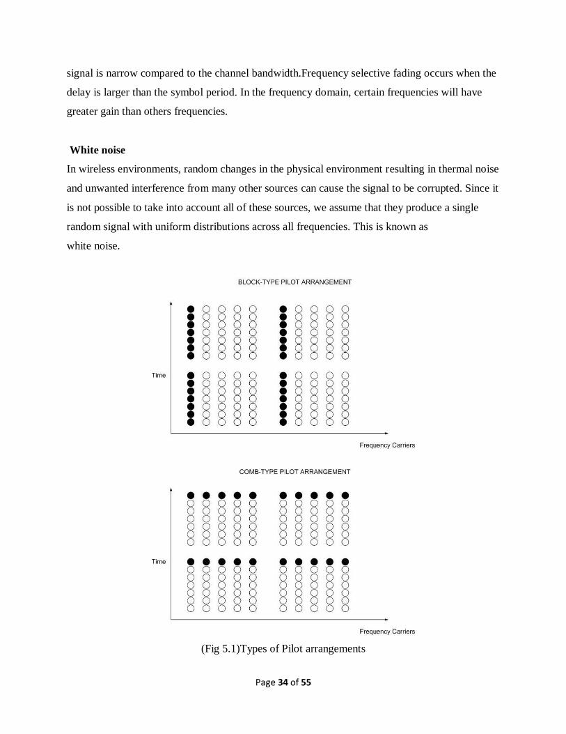
the received signal. In this chapter we have investigated two types of pilot arrangements: Block

type and Comb type.

5.2 SYSTEM ENVIRONMENT

Wireless

The system environment we will be considering in this thesis will be wireless indoor and urban

areas, where the path between transmitter and receiver is blocked by various objects and

obstacles. For example, an indoor environment has walls and furniture, while the outdoor

environment contains buildings and trees. This can be characterized by the impulse response in a

wireless environment.

Multipath Fading

Most indoor and urban areas do not have direct line of sight propagation between the transmitter

and receiver. Multi-path occurs as a result of reflections and diffractions by objects of the

transmitted signal in a wireless environment. These objects can be such things as buildings and

trees. The reflected signals arrive with random phase offsets as each reflection follows a

different path to the receiver. The signal power of the waves also decreases as the distance

increases. The result is random signal fading as these reflections destructively and constructively

superimpose on each other. The degree of fading will depend on the delay spread (or phase

offset) and their relative signal power.

Fading Effects due to Multi-path Fading

Time dispersion due to multi-path leads to either flat fading or frequency selective fading:

Flat fading occurs when the delay is less than the symbol period and affects all frequencies

equally. This type of fading changes the gain of the signal but not the spectrum. This is known as

amplitude varying channels or narrowband channels, since the bandwidth of the applied

of 55

signal is narrow compared to the channel bandwidth.Frequency selective fading occurs when the

delay is larger than the symbol period. In the frequency domain, certain frequencies will have

greater gain than others frequencies.

White noise

In wireless environments, random changes in the physical environment resulting in thermal noise

and unwanted interference from many other sources can cause the signal to be corrupted. Since it

is not possible to take into account all of these sources, we assume that they produce a single

random signal with uniform distributions across all frequencies. This is known as

white noise.

(Fig 5.1)Types of Pilot arrangements

of 55

5.3 CHANNEL ESTIMATION BASED ON BLOCK-TYPE PILOT

ARRANGEMENT

In block-type pilot based channel estimation, OFDM channel estimation symbols

are transmitted periodically, in which all sub-carriers are used as pilots. If the channel

is constant during the block, there will be no channel estimation error since the pilots

are sent at all carriers. The estimation can be performed by using either LSE or

MMSE .If inter symbol interference is eliminated by the guard interval, we write in

matrix notation:

Y=XFh+ W

= XH +W

where

of 55

5.4 CHANNEL ESTIMATION BASED ON COMB-TYPE

PILOT ARRANGEMENT

In comb-type based channel estimation, the Np pilot signals are uniformly inserted

into X(k) according to following equation:

L = number of carriers/Np

xp(m) is the mth pilot carrier value.

5.5 PILOT BASED CHANNEL ESTIMATION

The following estimators use on pilot data that is known to both transmitter and receiver as a

reference in order to track the fading channel. The estimators use block based pilot symbols,

meaning that pilot symbols are sent across all sub-carriers periodically during channel

estimation. This estimate is then valid for one OFDM/MC-CDMA frame before a new channel

estimate will be required.

Since the channel is assumed to be slow fading, our system will assume a frame format,

transmitting one channel estimation pilot symbol, followed by five data symbols, as indicated in

the time frequency lattice shown in adjoining figure . Thus each channel estimate will be used

for the following five data symbols.

of 55

(Fig 5.2) Block type pilot estimation

5.6 LEAST SQUARES ESTIMATOR

The simplest channel estimator is to divide the received signal by the input signals, which should

be known pilot symbols. This is known as the Least Squares (LS) Estimator and can simply be

expressed as:

HLS =y/x

This is the most naive channel estimator as it works best when no noise is present in the channel.

When there is no noise the channel can be estimated perfectly. This estimator is equivalent to a

zero-forcing estimatorThe main advantage is its simplicity and low complexity. It only requires

a single division per sub-carrier. The main disadvantage is that it has high mean-square error.

This is due to its use of an oversimplified channel and does not make use of the frequency and

time correlation of the slow fading channel.

of 55

An improvement to the LS estimator would involve making use of the channel statistics. We

could modify the LS estimator by tracking the average of the most recently estimated channel

vectors.

We have to minimize

For minimization of J we have to differentiate J with respect to H

5.7 LINEAR MINIMUM MEAN SQUARE ERROR ESTIMATOR

The Linear Minimum Mean Squares Error (LMMSE) Estimator minimizes the mean square error

(MSE) between the actual and estimated channel by using the frequency correlation of the slow

fading channel. This is achieved through a optimizing linear transformation applied to the LS

estimator described in the previous section. From adaptive filter theory, the optimum

solution in terms of the MSE is given by the Wiener-Hopf equation:

where X is a matrix conatining the transmitted signalling points on its diagonal,

of 55

2

is the additive noise variance. The matrix Rhhls is the cross correlation between channel

attenuation vector h and the LS estimate hls and Rhlshls is the auto correlation matrix of the LS

estimate hls, given by

Since white noise is uncorrelated with the channel attenuation, the cross correlation between the

channel h and noisy channel hls is the same as the autocorrelation of the channel h. Thus we can

replace Rhhls with Rhh. Also the autocorrelation of Rhlshls is equavalent to Rhh plus the noise

power (2)

and signal power. So the estimator can be expressed as:

5.8 SYSTEM CONSIDERATIONS

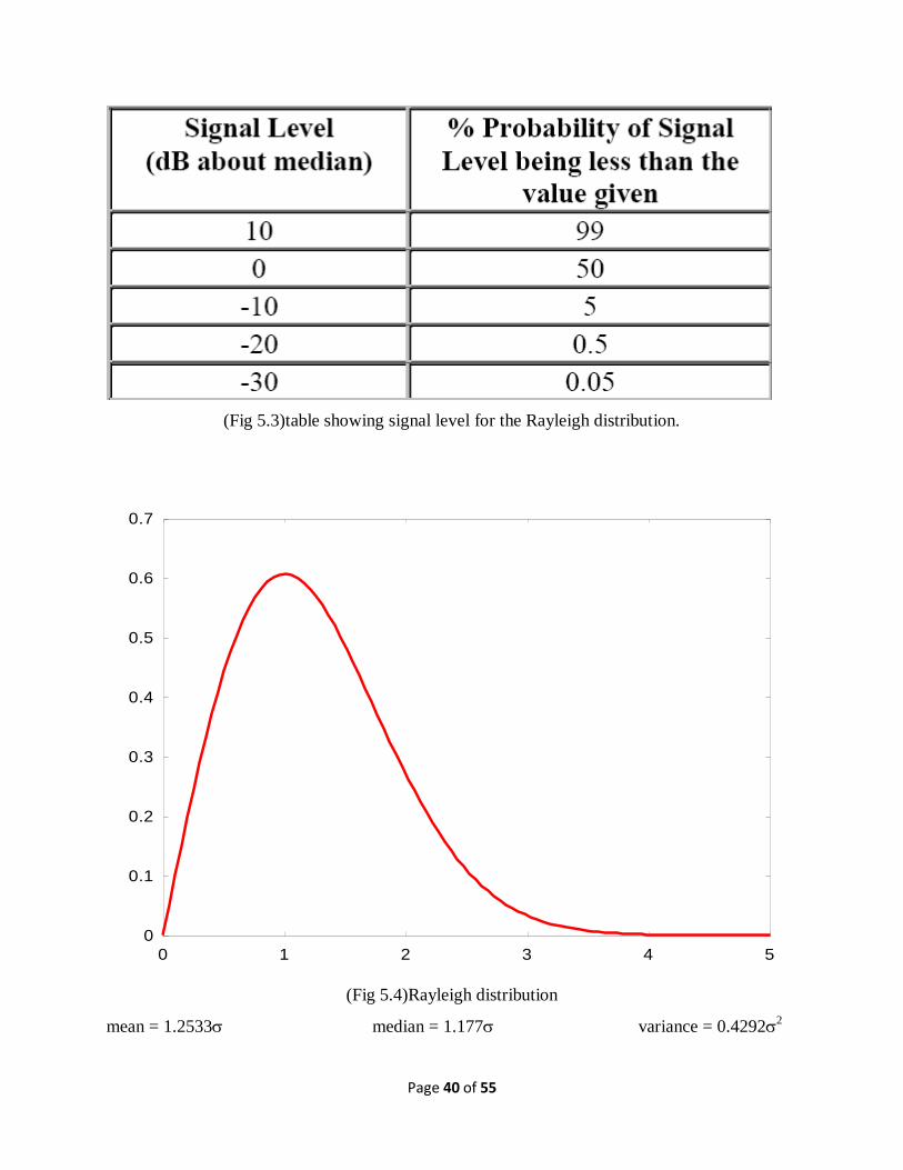
RAYLEIGH FADING

The Rayleigh distribution is commonly used to describe the statistical time varying nature of the

received envelope of a flat fading signal, or the envelope of an individual multipath component.

The envelope of the sum of two quadrature Gaussian noise signals obeys a Rayleigh distribution.

is the rms value of the received voltage before envelope detection, and 2 is the time-

average power of the received signal before envelope detection.

It describes the probability of the signal level being received due to fading. Table shows the

probability of the signal level for the Rayleigh distribution.

00

0)2

exp()( 2

2

2

r

rrr

rp

of 55

(Fig 5.3)table showing signal level for the Rayleigh distribution.

0

0.1

0.2

0.3

0.4

0.5

0.6

0.7

0 1 2 3 4 5

(Fig 5.4)Rayleigh distribution

mean = 1.2533 median = 1.177 variance = 0.42922

of 55

Doppler Shift

When a wave source and a receiver are moving relative to one another the frequency of the

received signal will not be the same as the source. When they are moving toward each other the

frequency of the received signal is higher than the source, and when they are moving away from

each other the frequency decreases. This is called the Doppler’s effect. An example of this is the

change of pitch in a car’s horn as it approaches then passes by. This effect becomes important

when developing mobile radio systems.

The amount the frequency changes due to the Doppler effect depends on the relative motion

between the source and receiver and on the speed of propagation of the wave. The Doppler shift

in frequency can be written as:

where Δf is the change in frequency of the source seen at the receiver,

f0 is the frequency of the source,

v is the speed difference between the source and transmitter,

and c is the speed of light

Assumptions on channel

To simplify our simulated channel, the following assumptions were made:

The impulse response is shorter than the Cyclic Prefix. Therefore, there is no ISI and ICI

and the channel is therefore diagonal.

The channel is a synchronised, sample spaced channel.

Channel noise is additive, white and complex Gaussian.

The fading on the channel is slow enough to be considered constant during one OFDM

frame

of 55

CHAPTER-6

SIMULATIONS AND RESULTS

of 55

6.1 Simulation Results for single bit without noise OFDM :

Transmission data bit=1

Received data bit after OFDM simulation=1

So, no error. Simulation was successful.

6.2 Simulation Results for multiple bit without noise OFDM (10bits to 10^5

bits): (model simulation)

Transmission data=[1011001010]

Received data after OFDM simulation=[1011001010]

Error bit count=0

Simulation was successful.

6.3 Simulation Results for multiple bit with noise(AWGN) OFDM (10bits to

10^5 bits): (model simulation)

SNR=12

Transmission data=[1011001010]

Received data after OFDM simulation=[1101011010]

Error bit count=3

As noise is introduced, error in transmission of few of the bits. Simulation was successful.

6.4 Simulation Results for multiuser without noise MC-CDMA (10bits to

10^4 bits): (model simulation)

Transmission data=

of 55

Received data after MC-CDMA simulation=

No. of users=8

Error in all 8 users =0

6.5 Simulation Results for single user with noise MC-CDMA (10bits to 10^4

bits):

BER Vs SNR plot (fig 6.1)

of 55

6.6 Simulation Results for multiuser with noise MC-CDMA (10bits to 10^4

bits): (model simulation )

For 10 000 bits

No. of users=8

User wise BER Vs SNR plot (fig 6.2)

of 55

Comparison of all the 8 users:

BER Vs SNR plot (fig 6.3)

of 55

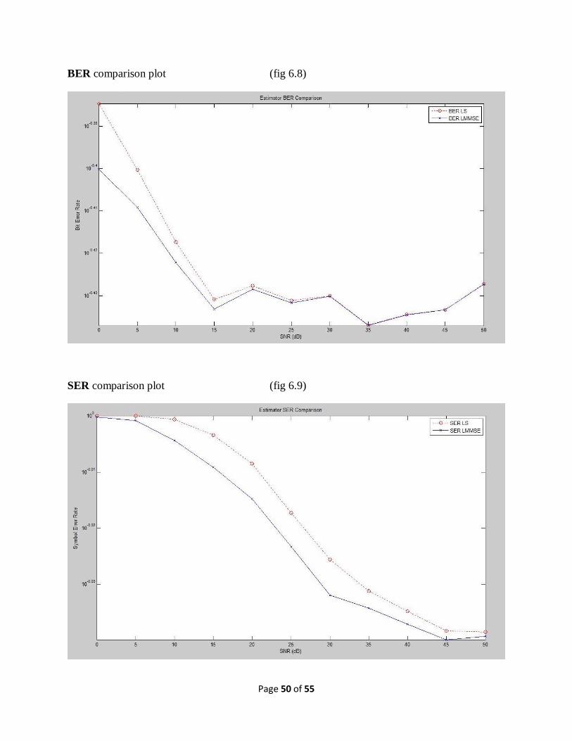
6.7 Simulation Results for channel estimation in MC-CDMA (10bits to 10^3

bits): (model simulation )

For 300 bits

Comparison between LS estimator and LMMSE estimator

MSE comparison plot (fig 6.4)

of 55

BER comparison plot (fig 6.5)

SER comparison plot (fig 6.6)

of 55

For 1000 bits

Comparison between LS estimator and LMMSE estimator

MSE comparison plot (fig 6.7)

of 55

BER comparison plot (fig 6.8)

SER comparison plot (fig 6.9)

of 55

CHAPTER-7

CONCLUSION

of 55

CONCLUSION

In this project we have simulated successively single bit without noise OFDM

system , multiple bit without noise OFDM system , multiple bit with noise OFDM

system for single user.

Then we simulated OFDM system for multiple user with and without noise. then

we simulated MC- CDMA systems, the BER Vs SNR plots for the previously

mentioned systems were obtained and were found to be satisfactory.

Then the simulation of channel estimation was carried out using LS and LMMSE

estimators and the MSE,BER and SER plots were obtained.

of 55

REFERENCES

[1] Rappaport, T., Wireless Communication: Principles and Practice. New Jersey: Prentice Hall,

1996.

[2] A Study of Channel Estimation in OFDM Systems Sinem Coleri, Mustafa Ergen,Anuj Puri,

Ahmad Bahai

[3] Proakis, J., Digital Communications. New York: McGraw-Hill, 1998.

[4]A.G. Orozco-Lugo, M. M. Lara, and D. C. McLernon, “Channel estimation using

implicit training,” IEEE Trans. on Sig. Processing, vol. 52, no.1, pp. 240-254, Jan.

2004

[5] Weinstein, S. and Ebert, P., “Data Transmission by Frequency Division Multiplexing using

the Discrete Fourier Transform.” IEEE Transaction Communication Technology vol. COM-19,

(October 1971): pp. 628-634.

[6] M. Hsieh and C. Wei, Channel estimation for OFDM systems based on comb type pilot

arrangement in frequency selective fading channels, in IEEE Transactions on Consumer

Electronics, vol. 44, no.1, February 1998.

[7] Channel Estimation and Equalization based on Implicit Training in OFDM Systems Jinesh P.

Nair and R. V. Raja Kumar G.S. Sanyal School of Telecommunications

[8] Hirosaki, B., “An analysis of automatic equalizers for orthogonally multiplexed QAM

systems,” IEEE Transaction Communication Technology. vol. COM-28, (January 1980): pp. 73-

83

[9 ]J.-J van de Beek, O. Edfors, M. Sandell, S.K. Wilson and P.O. Borjesson, On channel

estimation in OFDM systems, in Proc. IEEE 45th Vehicular Technology Conference, Chicago,

IL, Jul. 1995, pp. 815-819.

[10] Ketel, I., “The Multitone Channel.” IEEE Transaction on Communication vol. 37, (February

1989): pp. 119-124.

[11] Fazel, K. and Fettis, G., “Performance of an Efficient Parallel Data Transmission System”

IEEE Transaction Communication Technology (December 1967): pp. 805-813.46

[12] Meyr, H., Moeneclaey, M. and Fechtel, S. A., Digital Communication Receivers. John

Wiley and Sons, 1998

of 55

[13] Li, Y., Seshadri, N. and Ariyavisitakul, S., “Channel Estimation for OFDM systems with

transmitter diversity in mobile wireless channels.” IEEE J. Select. Areas Communication (March

1999): pp. 461-470.

[14] Y. Li, Pilot-Symbol-Aided Channel Estimation for OFDM in Wireless Systems, in IEEE

Transactions on Vehicular Technology, vol. 49, no.4, July 2000

[15] Y.Zhao and A. Huang, A novel channel estimation method for OFDM Mobile

Communications Systems based on pilot signals and transform domain processing, in Proc. IEEE

47th Vehicular Technology Conference, Phoenix, USA, May 1997, pp. 2089-2093

[16] Cavers, J. K., “An analysis of Pilot symbol assisted modulation for Rayeigh fading

channels.” IEEE Transaction on Vehicular Technology. vol. 40(4), (November 1991):pp.686-

693.

[17] Moon, JAe Kyoung and Choi, Song In., “Performance of channel estimation methods for

OFDM systems in multipath fading channels.” IEEE Transaction on Communication Electronics.

vol.46, (February 2000): pp. 161-170

[18] Tufvesson, F., Faulkner, M., Hoeher, P. and Edfors, O., “OFDM Time and Frequency

Synchronization by spread spectrum pilot technique.” 8th IEEE Communication Theory Mini

Conference in conjunction to ICC’99, Vancouver, Canada, (June 1999): pp. 115- 119.

[19] Tufvesson, F. and Hoeher, P., “Channel Estimation using Superimposed pilot Sequences,”

IEEE Trans. Communication (March 2000).

[20]O. Edfors, M. Sandell, J. Beek, S. K. Wilson, and P. O. Borjesson, “OFDM channel

estimation by singular value decomposition,” IEEE Trans. On Communications, vol. 46, no. 7,

pp.931-939, July 1998.

[21] Xiaoqiand, Ma., Kobayashi, H. and Schwartz, Stuart C., “An EM Based Estimation of

OFDM Signals.” IEEE Transaction Communication. (2002). [22] Edfors, O., Sandell, M.,Van de

Beek, J. J., Wilson, S. K. and Boriesson, P. O., “Analysis of DFT-based channel estimators for

OFDM.” Vehicular Technology Conference. (July 1995).

[22] James Shen, Mathew Liu ,”a thesis on OFDM channel estimation and equalization with

MATLAB”. (http://www.geocities.com/ofdm99).

[23] Nathan Yee, Jean-Paul Linnartz and Gerhard Fettweis , “multi-carrier CDMA in indoor

wireless radio networks”

of 55

[24] Jean-Paul M. G. Linnartz, Senior Member, IEEE, ”Performance Analysis of Synchronous

MC-CDMA in Mobile Rayleigh Channel With Both Delay and Doppler Spreads”.

[25] Bong-Soo Lee , Sin-Chong Park,” Design and Performance Analysis of the MC-CDMA”.

[26] Dr. Mohab Mangoud ,Yasser Ahmed Abbady ,” OFDM Basics Report”.

CHANNEL ESTIMATION IN MULTI CARRIER CODE DIVISION MULTIPLE...

Documents

Transcript of CHANNEL ESTIMATION IN MULTI CARRIER CODE DIVISION MULTIPLE...