Channel Estimation and Equalization for Cooperative ... · PDF fileChannel Estimation and...
135
Channel Estimation and Equalization for Cooperative Communication by Hakam Mheidat A thesis presented to the University of Waterloo in fulfillment of the thesis requirement for the degree of Doctor of Philosophy in Electrical and Computer Engineering Waterloo, Ontario, Canada, 2006 © Hakam Mheidat 2006
Transcript of Channel Estimation and Equalization for Cooperative ... · PDF fileChannel Estimation and...
Channel Estimation and Equalization for
Cooperative Communication
by
Hakam Mheidat
A thesis
presented to the University of Waterloo
in fulfillment of the
thesis requirement for the degree of
Doctor of Philosophy
in
Electrical and Computer Engineering
Waterloo, Ontario, Canada, 2006
© Hakam Mheidat 2006

ii
I hereby declare that I am the sole author of this thesis. This is a true copy of the thesis,
including any required final revisions, as accepted by my examiners.
I understand that my thesis may be made electronically available to the public.

iii
Abstract
The revolutionary concept of space-time coding introduced in the last decade has
demonstrated that the deployment of multiple antennas at the transmitter allows for
simultaneous increase in throughput and reliability because of the additional degrees of
freedom offered by the spatial dimension of the wireless channel. However, the use of
antenna arrays is not practical for deployment in some practical scenarios, e.g., sensor
networks, due to space and power limitations.
A new form of realizing transmit diversity has been recently introduced under the name of
user cooperation or cooperative diversity. The basic idea behind cooperative diversity rests
on the observation that in a wireless environment, the signal transmitted by the source node is
overheard by other nodes, which can be defined as “partners” or “relays”. The source and its
partners can jointly process and transmit their information, creating a “virtual antenna array”
and therefore emulating transmit diversity.
Most of the ongoing research efforts in cooperative diversity assume frequency flat
channels with perfect channel knowledge. However, in practical scenarios, e.g. broadband
wireless networks, these assumptions do not apply. Frequency-selective fading and imperfect
channel knowledge should be considered as a more realistic channel model. The
development of equalization and channel estimation algorithms play a crucial element in the
design of digital receivers as their accuracy determine the overall performance.
This dissertation creates a framework for designing and analyzing various time and
frequency domain equalization schemes, i.e. distributed time reversal (D-TR) STBC,
distributed single carrier frequency domain (D-SC-FDE) STBC, and distributed orthogonal
frequency division multiplexing (D-OFDM) STBC schemes, for broadband cooperative
communication systems. Exploiting the orthogonally embedded in D-STBCs, we were able
iv
to maintain low-decoding complexity for all underlying schemes, thus, making them
excellent candidates for practical scenarios, such as multi-media broadband communication
systems.
Furthermore, we propose and analyze various non-coherent and channel estimation
algorithms to improve the quality and reliability of wireless communication networks.
Specifically, we derive a non-coherent decoding rule which can be implemented in practice
by a Viterbi-type algorithm. We demonstrate through the derivation of a pairwise error
probability expression that the proposed non-coherent detector guarantees full diversity.
Although this decoding rule has been derived assuming quasi-static channels, its inherent
channel tracking capability allows its deployment over time-varying channels with a
promising performance as a sub-optimal solution. As a possible alternative to non-coherent
detection, we also investigate the performance of mismatched-coherent receiver, i.e.,
coherent detection with imperfect channel estimation. Our performance analysis
demonstrates that the mismatched-coherent receiver is able to collect the full diversity as its
non-coherent competitor over quasi-static channels.
Finally, we investigate and analyze the effect of multiple antennas deployment at the
cooperating terminals assuming different relaying techniques. We derive pairwise error
probability expressions quantifying analytically the impact of multiple antenna deployment at
the source, relay and/or destination terminals on the diversity order for each of the relaying
methods under consideration.

v
Acknowledgments
I would like to express my sincere gratitude to my supervisor Professor Murat Uysal whose
valuable support, advice and comments made this work possible. Murat is truly an endless
source of creative ideas. His tireless efforts, advice and guidance helped me learn valuable
lessons which would definitely help me greatly in my future career.
Many thanks are due to the members of my doctoral committee, Prof. Amir K. Khandani,
Prof. Samir Elhedhli, Prof. M. Oussama Damen, and Prof. Liang-Liang Xie for their valuable
time and efforts. It has been a great honor and pleasure to have Prof. Ravi Adve from the
University of Toronto as my external committee member. I am truly honored to have such a
great examining committee.
I would like to thank my family, my parents, my brothers and sisters and their families for
all of the love, support, and encouragement they have given me throughout this process. I
would also like to thank my mother in law Ae ok Chun for treating me like her own son and
supporting me. Special thanks to Y. J. Kim, C. D. Park, and Silver Mirror Kim for their
support. I have been truly blessed and am extremely grateful to have the family that I have.
Finally, I would like to thank my wife, Hyunjoo Kim, who has been my life glory and
motivation. I would like to thank her for her support, help and patience in the process of this
work. No one could ask for more than she gives me everyday; she is truly God's miracle in
my life.
vi
Dedication
To my parents: Mohammed and Hekmat
and
To my beloved wife: Hyunjoo
vii
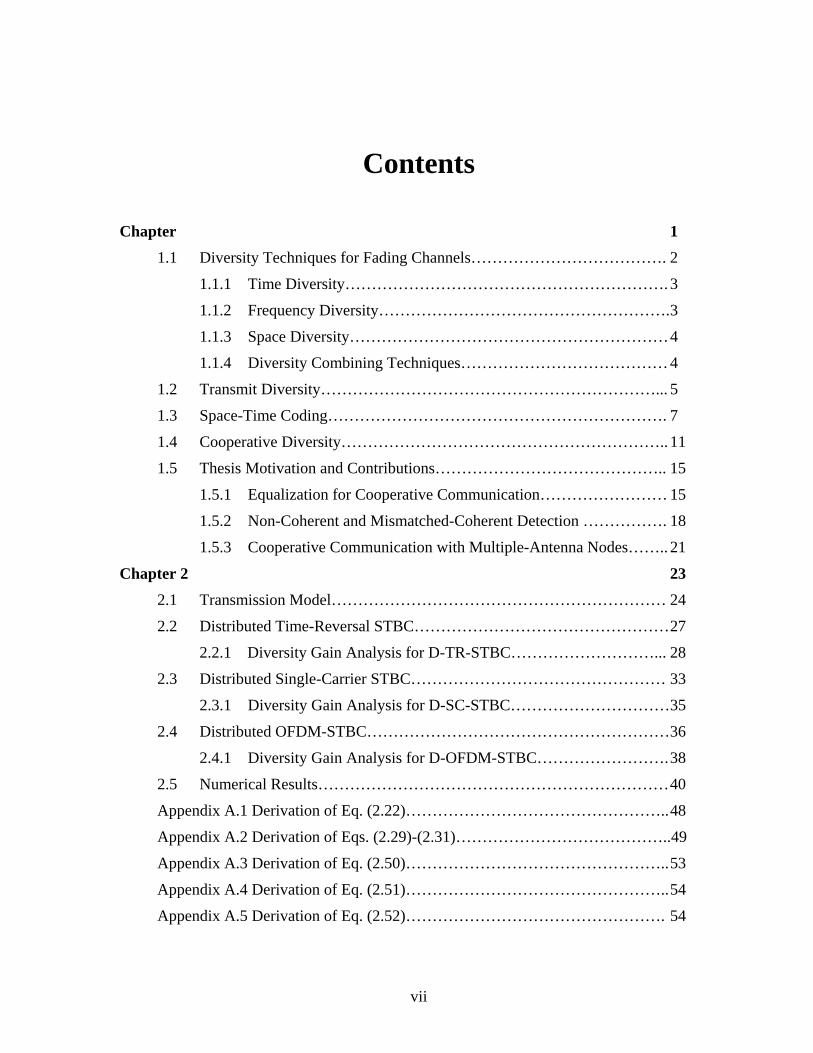
Contents
Chapter 1 1.1 Diversity Techniques for Fading Channels………………………………. 2
1.1.1 Time Diversity……………………………………………………. 3
1.1.2 Frequency Diversity………………………………………………. 3
1.1.3 Space Diversity…………………………………………………… 4
1.1.4 Diversity Combining Techniques………………………………… 4
1.2 Transmit Diversity………………………………………………………... 5
1.3 Space-Time Coding………………………………………………………. 7
1.4 Cooperative Diversity…………………………………………………….. 11
1.5 Thesis Motivation and Contributions…………………………………….. 15
1.5.1 Equalization for Cooperative Communication…………………… 15
1.5.2 Non-Coherent and Mismatched-Coherent Detection ……………. 18
1.5.3 Cooperative Communication with Multiple-Antenna Nodes…….. 21
Chapter 2 23 2.1 Transmission Model……………………………………………………… 24
2.2 Distributed Time-Reversal STBC………………………………………… 27
2.2.1 Diversity Gain Analysis for D-TR-STBC………………………... 28
2.3 Distributed Single-Carrier STBC………………………………………… 33
2.3.1 Diversity Gain Analysis for D-SC-STBC………………………… 35
2.4 Distributed OFDM-STBC………………………………………………… 36
2.4.1 Diversity Gain Analysis for D-OFDM-STBC……………………. 38
2.5 Numerical Results………………………………………………………… 40
Appendix A.1 Derivation of Eq. (2.22)………………………………………….. 48
Appendix A.2 Derivation of Eqs. (2.29)-(2.31)…………………………………..49
Appendix A.3 Derivation of Eq. (2.50)………………………………………….. 53
Appendix A.4 Derivation of Eq. (2.51)………………………………………….. 54
Appendix A.5 Derivation of Eq. (2.52)…………………………………………. 54
viii
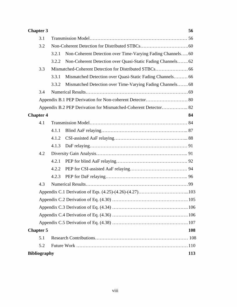
Chapter 3 56 3.1 Transmission Model……………………………………………………… 56
3.2 Non-Coherent Detection for Distributed STBCs…………………………. 60
3.2.1 Non-Coherent Detection over Time-Varying Fading Channels….. 60
3.2.2 Non-Coherent Detection over Quasi-Static Fading Channels……. 62
3.3 Mismatched-Coherent Detection for Distributed STBCs………………… 66
3.3.1 Mismatched Detection over Quasi-Static Fading Channels……… 66
3.3.2 Mismatched Detection over Time-Varying Fading Channels……. 68
3.4 Numerical Results………………………………………………………… 69
Appendix B.1 PEP Derivation for Non-coherent Detector……………………… 80
Appendix B.2 PEP Derivation for Mismatched-Coherent Detector…………….. 82
Chapter 4 84 4.1 Transmission Model……………………………………………………… 84
4.1.1 Blind AaF relaying……………………………………………….. 87
4.1.2 CSI-assisted AaF relaying………………………………………... 88
4.1.3 DaF relaying……………………………………………………… 91
4.2 Diversity Gain Analysis………………………………………………….. 91
4.2.1 PEP for blind AaF relaying………………………………………. 92
4.2.2 PEP for CSI-assisted AaF relaying………………………………. 94
4.2.3 PEP for DaF relaying…………………………………………….. 96
4.3 Numerical Results………………………………………………………… 99
Appendix C.1 Derivation of Eqs. (4.25)-(4.26)-(4.27)…………………………...103
Appendix C.2 Derivation of Eq. (4.30) …………………………………………. 105
Appendix C.3 Derivation of Eq. (4.34) …………………………………………. 106
Appendix C.4 Derivation of Eq. (4.36) …………………………………………. 106
Appendix C.5 Derivation of Eq. (4.38) …………………………………………. 107
Chapter 5 108 5.1 Research Contributions…………………………………………………… 108
5.2 Future Work ……………………………………………………………… 110
Bibliography 113
ix
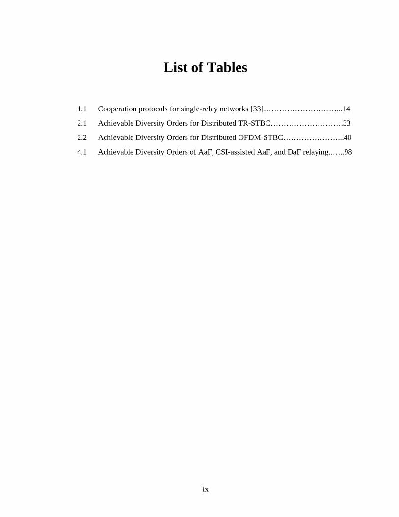
List of Tables
1.1 Cooperation protocols for single-relay networks [33]……………………. …...14
2.1 Achievable Diversity Orders for Distributed TR-STBC……………………….33
2.2 Achievable Diversity Orders for Distributed OFDM-STBC…………………...40
4.1 Achievable Diversity Orders of AaF, CSI-assisted AaF, and DaF relaying..…..98
x
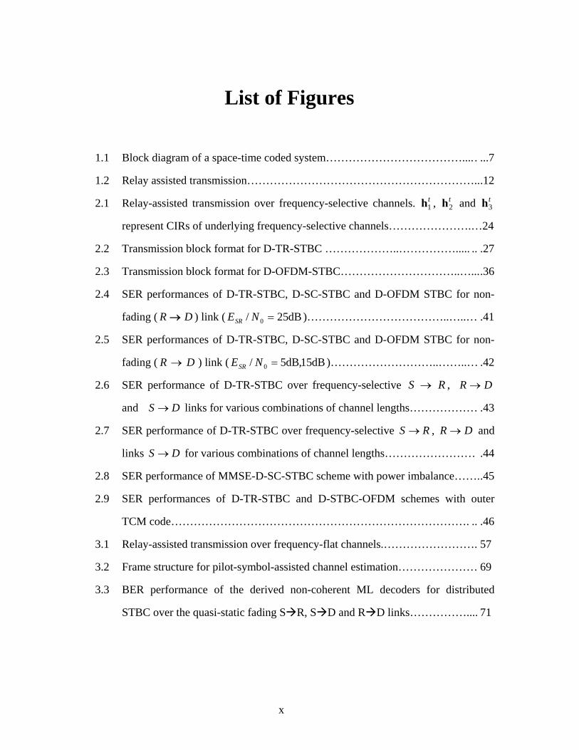
List of Figures
1.1 Block diagram of a space-time coded system……………………………….... . ...7
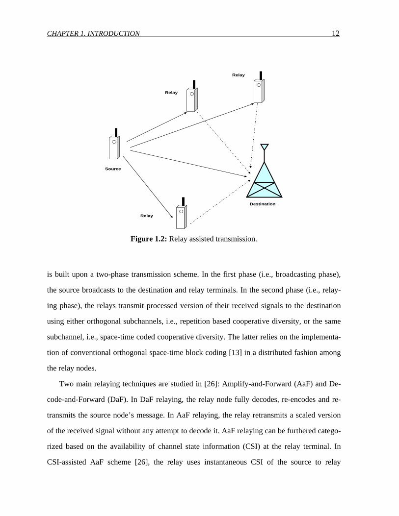
1.2 Relay assisted transmission……………………………………………………...12
2.1 Relay-assisted transmission over frequency-selective channels. t1h , t
2h and t3h
represent CIRs of underlying frequency-selective channels………………….…24
2.2 Transmission block format for D-TR-STBC ………………..……………..... .. .27
2.3 Transmission block format for D-OFDM-STBC…………………………..…....36
2.4 SER performances of D-TR-STBC, D-SC-STBC and D-OFDM STBC for non-
fading ( DR → ) link ( dB25/ 0 =NESR )………………………………..…..… .41
2.5 SER performances of D-TR-STBC, D-SC-STBC and D-OFDM STBC for non-
fading ( DR → ) link ( dB15,dB5/ 0 =NESR )………………………..……..… .42
2.6 SER performance of D-TR-STBC over frequency-selective ,RS → DR →
and DS → links for various combinations of channel lengths……………… .43
2.7 SER performance of D-TR-STBC over frequency-selective RS → , DR → and
links DS → for various combinations of channel lengths…………………… .44
2.8 SER performance of MMSE-D-SC-STBC scheme with power imbalance……..45
2.9 SER performances of D-TR-STBC and D-STBC-OFDM schemes with outer
TCM code……………………………………………………………………. .. .46
3.1 Relay-assisted transmission over frequency-flat channels.……………………. 57
3.2 Frame structure for pilot-symbol-assisted channel estimation………………… 69
3.3 BER performance of the derived non-coherent ML decoders for distributed
STBC over the quasi-static fading S R, S D and R D links…………….... 71
xi
3.4.a BER performance of the proposed non-coherent ML decoder given by Eq. (3.24)
and its recursive implementation given by Eq.(3.29) over the quasi-static fading
S R and S D links……………………………………………………….….. 72
3.4.b Effective diversity order of distributed STBC………………………………… 73
3.5 Performance comparison of mismatched-coherent and non-coherent decoders for
distributed STBC over quasi-static fading links………………………………. 75
3.6 BER performance comparison of the non-coherent optimal decoder, non coherent
recursive decoder, and mismatched-coherent decoder for distributed STBC with
non-fading R D link. Normalized Doppler values for S R and S D links are
01.0== SDSR fTfT …………………………………………………………… .. 76
3.7 BER performance comparison of the non-coherent recursive decoder and
mismatched coherent decoder for distributed STBC with fading R D link.
Normalized Doppler values for S R, R D and S D links
are =fT SRfT == RDfT 05.0,03.0,02.0,01.0=SDfT ………………………….. .. 77
3.8 BER vs. Doppler spread for distributed STBC with non-coherent recursive de-
coder and mismatched-coherent decoder……………………………………... . 79
4.1 Schematic representation of relay-assisted transmission with multi-antenna
nodes…………………………………………………………………………….85
4.2 SER performances of blind AaF scheme with multi-antenna nodes…………..100
4.3 SER performances of CSI-assisted AaF scheme with multi-antenna nodes…...101
4.4 SER performances of DaF scheme with multi-antenna nodes…………………102
xii
Abbreviations
AaF Amplify-and-forward
AWGN Additive white Gaussian noise
BER Bit error rate
CP Cyclic prefix
CSI Channel state information
DaF Decode-and-forward
DFT Discrete Fourier Transform
EDO The effective diversity order
EGC Equal gain combining
FFT Fast Fourier Transform
IFFT Inverse Fast Fourier Transform
i.i.d Identical independent distribution
LMMSE Linear minimum mean square error
MIMO Multiple-input-multiple-output
MISO Multi-input-single-output
MRC Maximal-ratio-combining
ML Maximum-likelihood
MLSE Maximum likelihood sequence estimation
OFDM Orthogonal frequency division multiplexing
PEP Pairwise error probability
PIR Pilot insertion rate
PSK Phase shift keying
QAM Quadrature amplitude modulation
SC Selection combining
SC-FDE Single-carrier frequency domain equalization
xiii
SER Symbol error rate
SIMO Single-input-multi-output
SNR Signal-to-Noise Ratio
STBC Space-time block coding
STTC Space-time trellis coding
TCM Trellis-coded modulation
TR Time reversal
ZP Zero-padding
xiv
Notations
(.)∗ Conjugate operation Τ(.) Transpose operation Η(.) Conjugate transpose operation
[.]E Expectation operation
⋅tr Trace operation
lk ,].[ The (k,l)th entry of a matrix
k[.] The kth entry of a vector
. The absolute value
⋅ Euclidean norm of a vector
⊗ Kronecker product
∗ Convolution operation
JI The identity matrix of size J
VV×0 All-zero matrix of size VV × .
Q JJ × FFT matrix whose (l,k) element is given by
)/ 2exp(/1),( JkljJkl π−=Q where 1,0 −≤≤ Jkl
(.)Γ The gamma function
(.)iE The exponential-integral function
⎡ ⎤. The ceiling function
( )ωYΦ The characteristic functions of Y
Q(.) The Gaussian-Q function
det(.) The determinant of a matrix
( ).diag The diagonal of a matrix
( ).,.Γ The incomplete gamma function
ln(.) The Natural logarithm
1
Chapter 1
Introduction
A quick glimpse of recent technological history reveals out that mobile communication
systems create a new generation roughly every 10 years. First-generation analogue systems
were introduced in the early 1980’s, then second-generation (2G) digital systems came in the
early 1990’s. Now third-generation (3G) systems are slowly unfolding all over the world
while intensive conceptual and research work toward the definition of a future system has
been already started.
2G systems, such as GSM and IS-95, were essentially designed for voice and low data rate
applications. In an effort to address customer demands for high-speed data communication,
telecommunication companies have been launching 3G systems where the business focus has
shifted from voice services to multimedia communication applications over the Internet. De-
spite the increasing penetration rate of 3G systems in the wireless market, 3G networks are
challenged primarily in meeting the requirements imposed by the ever-increasing demands of
high-throughput multimedia and internet applications. Additionally, 3G systems consist pri-
marily of wide area networks and thus fall short of supporting heterogeneous networks, in-
cluding wireless local area networks (LANs) and wireless personal area networks (WPANs).
Several wireless technologies co-exist in the current market customized for different ser-
vice types, data rates, and users. The next generation systems also known as the fourth gen-
CHAPTER 1. INTRODUCTION 2
eration (4G) systems are envisioned to accommodate and integrate all existing and future
technologies in a single standard. The key feature of the 4G systems would be “high usabil-
ity” [1]; that is the user would be able to use the system at anytime, anywhere, and with any
technology. Users carrying an integrated wireless terminal would have access to a variety of
multimedia applications in a reliable environment at lower cost. To meet these demands, next
generation wireless communication systems must support high capacity and variable bit rate
information (adaptive) transmission with high bandwidth efficiency to conserve limited spec-
trum resources.
1.1 Diversity Techniques for Fading Channels
The characteristics of wireless channel impose fundamental limitations on the perform-
ance of wireless communication systems. The wireless channel can be investigated by com-
posing it into two parts, i.e., large-scale (long-term) impairments including path loss, shad-
owing and small-scale (short-term) impairment which is commonly referred as fading. The
former component is used to predict the average signal power at the receiver side and the
transmission coverage area. The latter is due to the multipath propagation which causes ran-
dom fluctuations in the received signal level and affects the instantaneous signal-to-noise ra-
tio (SNR).
For a typical mobile wireless channel in urban areas where there is no line of sight propa-
gation and the number of scatters is considerably large, the application of central limit theory
indicates that the complex fading channel coefficient has two quadrature components which
are zero-mean Gaussian random processes. As a result, the amplitude of the fading envelope
follows a Rayleigh distribution. In terms of error rate performance, Rayleigh fading converts
the exponential dependency of the bit-error probability on the SNR for the classical additive
CHAPTER 1. INTRODUCTION 3
white Gaussian noise (AWGN) channel into an approximately inverse linear one, resulting in
a large SNR penalty.
A common approach to mitigate the degrading effects of fading is the use of diversity
techniques. Diversity improves transmission performance by making use of more than one
independently faded version of the transmitted signal. If several replicas of the signals are
transmitted over multiple channels that exhibit independent fading with comparable
strengths, the probability that all the independently faded signal components experience deep
fading simultaneously is significantly reduced.
There are various approaches to extract diversity from the wireless channel. The most
common methods are briefly summarized as follows [2], [3], [4]:
1.1.1 Time Diversity
In this form of diversity, the same signal is transmitted in different time slots separated by
an interval longer than the coherence time of the channel. Channel coding in conjunction
with interleaving is an efficient technique to provide time diversity. In fast fading environ-
ments where the mobility is high, time diversity becomes very efficient. However, for slow-
fading channel (e.g., low mobility environments, fixed-wireless applications), it offers little
protection unless significant interleaving delays can be tolerated.
1.1.2 Frequency Diversity
In this form of diversity, the same signal is sent over different frequency carriers, whose
separation must be larger than the coherence bandwidth of the channel to ensure independ-
ence among diversity channels. Since multiple frequencies are needed, this is generally not a
bandwidth-efficient solution. A natural way of frequency diversity, which is sometimes re-
ferred to as path diversity, arises for frequency-selective channels. When the multipath delay
spread is a significant fraction of the symbol period, the received signal can be interpreted as
CHAPTER 1. INTRODUCTION 4
a linear combination of the transmitted signal weighted by independent fading coefficients.
Therefore, path diversity is obtained by resolving the multipath components at different de-
lays using a RAKE correlator [2], which is the optimum receiver in the MMSE sense de-
signed for this type of channels.
1.1.3 Space Diversity
In this form of diversity, which is also sometimes called as antenna diversity, the receiver
and/or transmitter uses multiple antennas. This technique is especially attractive since it does
not require extra bandwidth. To extract full diversity advantages, the spacing between an-
tenna elements should be wide enough with respect to the carrier wavelength. The required
antenna separation depends on the local scattering environment as well as on the carrier fre-
quency. For a mobile station which is near the ground with many scatters around, the channel
decorrelates over shorter distances, and typical antenna separation of half to one carrier
wavelength is sufficient. For base stations on high towers, a larger antenna separation of sev-
eral to tens of wavelengths may be required.
1.1.4 Diversity Combining Techniques
There exist different combining techniques, each of which can be used in conjunction
with any of the aforemetioned diversity forms. The most common diversity combining tech-
niques are selection, equal gain and maximal ratio combining [2]. Selection combining (SC)
is conceptually the simplest; it consists of selecting at each time, among the available diver-
sity branches (channels), the one with the largest value of SNR. Since it requires only a
measure of the powers received from each branch and a switch to choose among the
branches, it is relatively easy to implement. However, the fact that it disregards the informa-
tion obtained from all branches except the selected one indicates its non-optimality. In equal
gain combining (EGC), the signals at the output of diversity branches are combined linearly
CHAPTER 1. INTRODUCTION 5
and the phase of the linear combination are selected to maximize the SNR disregarding the
amplitude differences. Since each branch is combined linearly, compared to SC, EGC per-
forms better. In maximal-ratio-combining (MRC), the signals at the output of diversity
branches are again combined linearly and the coefficients of the linear combination are se-
lected to maximize the SNR regarding both the phase and the amplitude. The MRC outper-
forms the other two, since it makes use of the both fading amplitude and phase information.
However, the difference between EGC and MRC is not considerably large in terms of power
efficiency; therefore, EGC can be preferred where implementation costs are crucial. It should
be emphasized that the effectiveness of any diversity scheme rests on the availability of inde-
pendently faded versions of the transmitted signal so that the probability of two or more rele-
vant versions of the signal undergoing a deep fade is minimum. The reader can refer to [2]-
[4] and references therein for a broad overview of diversity combining systems.
1.2 Transmit Diversity
Space diversity, in the form of multiple antenna deployment at the receive side, has been
successfully used in uplink transmission (i.e., from mobile station to base station) of the cel-
lular communication systems. However, the use of multiple receive antennas at the mobile
handset in the downlink transmission (i.e., from base station to mobile station) is more diffi-
cult to implement because of size limitations and the expense of multiple down-conversion of
RF paths. This motivates the use of multiple transmit antennas at the base station in the
downlink. Since a base station often serves many mobile stations, it is also more economical
to add hardware and additional signal processing burden to base stations rather than the mo-
bile handsets. Despite its obvious advantages, transmit diversity has traditionally been
viewed as more difficult to exploit, in part because the transmitter is assumed to know less
about the channel than the receiver and in part because of the challenging signaling design
CHAPTER 1. INTRODUCTION 6
problem. Within the last decade, transmit diversity has attracted a great attention and practi-
cal solutions to realize transmit diversity advantages have been proposed [4].
The transmit diversity techniques can be classified into two broad categories based on the
need for channel state information at the transmit side: Close loop schemes and open loop
schemes. The first category uses feedback, either explicitly or implicitly, from the receiver to
the transmitter to configure the transmitter. Close loop transmit diversity has more power ef-
ficiency compared to open loop transmit diversity. However, it increases the overhead of
transmission and therefore is not bandwidth-efficient. Moreover, in practice, vehicle move-
ments or interference causes a mismatch between the state of the channel perceived by the
transmitter and that perceived by the receiver, making the feedback unreliable in some situa-
tions.
In open loop transmit diversity schemes feedback is not required. They use linear proc-
essing at the transmitter to spread the information across multiple antennas. At the receive
side, information is recovered by either linear processing or maximum-likelihood decoding
techniques. The first of such schemes was proposed by Wittneben [5], [6] where the operat-
ing frequency-flat fading channel is converted intentionally into a frequency-selective chan-
nel to exploit artificial path diversity by means of a maximum-likelihood decoder. It was
later shown in [7] that delay diversity schemes are optimal in providing diversity in the sense
that the diversity advantage experienced by an optimal receiver is equal to the number of
transmit antennas.
The linear filtering used to create delay diversity at the transmitter can be viewed as a
channel code which takes binary or integer input and creates real-valued output. Therefore,
from a coding perspective, delay diversity schemes correspond to repetition codes and lead to
the natural question as to whether more sophisticated codes might be designed. The challenge
CHAPTER 1. INTRODUCTION 7
of designing channel codes for multiple-antenna systems has led to the introduction of so-
called space-time trellis codes by Tarokh, Seshadri and Calderbank [8].
1.3 Space-Time Coding
Space-time trellis codes (STTCs) combine the channel code design with symbol mapping
onto multiple transmit antennas. The data symbols are cleverly coded across space and time
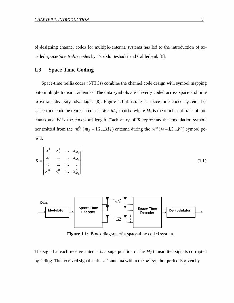
to extract diversity advantages [8]. Figure 1.1 illustrates a space-time coded system. Let
space-time code be represented as a SMW × matrix, where MS is the number of transmit an-
tennas and W is the codeword length. Each entry of X represents the modulation symbol
transmitted from the thSm ( SS Mm ,...2,1= ) antenna during the thw ( Ww ,...2,1= ) symbol pe-
riod.
⎥⎥⎥⎥⎥
⎦
⎤
⎢⎢⎢⎢⎢
⎣
⎡
=
WM
WW
M
M
S
S
S
xxx
xxxxx
...:......:
......
...
21
221
112
11
X (1.1)
Data
Modulator
Space-Time Encoder
Space-Time Decoder Demodulator
Figure 1.1: Block diagram of a space-time coded system.
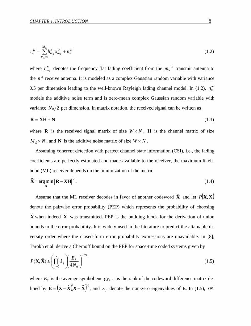
The signal at each receive antenna is a superposition of the MS transmitted signals corrupted
by fading. The received signal at the thn antenna within the thw symbol period is given by
CHAPTER 1. INTRODUCTION 8
wn
M
m
wm
nm
wn nxhr
S
SSS+= ∑
=1 (1.2)
where nmS
h denotes the frequency flat fading coefficient from the thSm transmit antenna to
the thn receive antenna. It is modeled as a complex Gaussian random variable with variance
0.5 per dimension leading to the well-known Rayleigh fading channel model. In (1.2), wnn
models the additive noise term and is zero-mean complex Gaussian random variable with
variance 20N per dimension. In matrix notation, the received signal can be written as
NXHR += (1.3)
where R is the received signal matrix of size NW × , H is the channel matrix of size
NM S × , and N is the additive noise matrix of size NW × .
Assuming coherent detection with perfect channel state information (CSI), i.e., the fading
coefficients are perfectly estimated and made available to the receiver, the maximum likeli-
hood (ML) receiver depends on the minimization of the metric 2 minargˆ XHRX
X−= . (1.4)
Assume that the ML receiver decodes in favor of another codeword X and let ( )XX ˆ,P
denote the pairwise error probability (PEP) which represents the probability of choosing
X when indeed X was transmitted. PEP is the building block for the derivation of union
bounds to the error probability. It is widely used in the literature to predict the attainable di-
versity order where the closed-form error probability expressions are unavailable. In [8],
Tarokh et al. derive a Chernoff bound on the PEP for space-time coded systems given by rN
Sr
jj N
EP−
=⎟⎟⎠
⎞⎜⎜⎝
⎛⎟⎟⎠
⎞⎜⎜⎝
⎛≤ ∏
00 4)ˆ,( λXX (1.5)
where SE is the average symbol energy, r is the rank of the codeword difference matrix de-
fined by ( )( )Η−−= XXXXE ˆˆ , and jλ denote the non-zero eigenvalues of E. In (1.5), rN
CHAPTER 1. INTRODUCTION 9
represents the diversity advantage, (i.e., the slope of the performance curve), while the prod-
uct of the non-zero eigen values of E denotes the coding advantage, (i.e., the horizontal shift
of the performance curve). The design criteria for space-time codes are further given in [8]:
Rank criterion: The code difference matrix, taken over all possible combinations of code
matrices, should be full rank. This criterion maximizes the diversity gain obtained from the
space-time code. The maximum diversity order that can be achieved is ),min( SMWr = .
Therefore, in order to achieve the maximum diversity of NM S × , E must be full rank.
Determinant criterion: The minimum determinant of E, taken over all possible combina-
tions of code matrices, should be maximized. This maximizes the coding gain. From (1.5), it
can be seen that the diversity gain term dominates the error probability at high SNR. There-
fore, the diversity gain should be maximized before the coding gain in the design of a space-
time code.
Based on the above criteria, Tarokh et al. [8] proposed some handcrafted codes which per-
form very well, within the 2-3 dB of the outage capacity derived in [9] for multiple antenna
systems. Since Tarokh’s pioneering work, there has been an extensive research effort in this
area for the design of optimized space-time trellis codes, a few to name are [10]-[12] among
many others.
Since every STTC has a well-defined trellis structure, standard soft decision techniques,
such as a Viterbi decoder, can be used at the receiver. For a fixed number of transmit anten-
nas, the decoding complexity of STTCs (measured by the number of trellis states at the de-
coder) increases exponentially with the transmission rate. Space-time block codes (STBCs)
[13]-[15] were proposed as an attractive alternative to its trellis counterpart with a much
lower decoding complexity. These codes are defined by a mapping operation of a block of
input symbols into the space and time domains, transmitting the resulting sequences from
different antennas simultaneously. Tarokh et al.’s work in [13] was inspired by Alamouti’s
CHAPTER 1. INTRODUCTION 10
early work [15], where a simple two-branch transmit diversity scheme was presented and
shown to provide the same diversity order as MRC with two receive antennas. Alamouti’s
scheme is appealing in terms of its performance and simplicity. It requires a very simple de-
coding algorithm based only on linear processing at the receiver. STBCs based on orthogonal
designs [13] generalizes Alamouti’s scheme to an arbitrary number of transmit antennas still
preserving the decoding simplicity and are able to achieve the full diversity at full transmis-
sion rate for real signal constellations and at half rate for complex signal constellations such
as QAM or PSK. Over the last few years several contributions have been made to further im-
prove the data rate of STBCs, e.g., [16], [17] and the references therein.
Super-orthogonal space-time trellis coding (SO-STTC) [18] is another class of space-time
code family. It combines set-partitioning with a super set of orthogonal STBC. While provid-
ing full-diversity and full-rate, the structure of these new codes allows the coding gain to be
improved over traditional STTC constructions. The underlying orthogonal structure of these
codes can be further exploited to decrease the decoding complexity in comparison to original
STTC designs. Another class of space-time codes is linear dispersion codes (LDC) [19].
Original LDCs have been original designed to maximize capacity gains and subsume spatial
multiplexing, which is a transmission technique offers a linear (in the number of transmit-
receive antenna pairs) increase in the transmission rate (or capacity) for the same bandwidth
and with no additional power expenditure, and STBCs as special cases. This code family is
able to provide an efficient trade-off between multiplexing and diversity gains for arbitrary
numbers of transmit and receive antennas [20].
As evidenced by the literal explosion of research papers on the topic, space-time coding
and its various combinations are becoming well understood in the research community. A
detailed treatment of space-time coding can be found in recently published text-books, e.g.,
[21], [22], [23].
CHAPTER 1. INTRODUCTION 11
1.4 Cooperative Diversity
Space-time coding techniques are quite attractive for deployment in the cellular applica-
tions at base stations and have been already included in the 3rd generation wireless standards.
Although transmit diversity is clearly advantageous on a cellular base station, it may not be
practical for other scenarios. Specifically, due to size, cost, or hardware limitations, a wire-
less device may not be able to support multiple transmit antennas. Examples include mobile
terminals and wireless sensor networks which are gaining popularity in the recent years.
In order to overcome these limitations, yet still emulate transmit antenna diversity, a new
form of realizing spatial diversity has been recently introduced under the name of user coop-
eration or cooperative diversity [24]-[28]. The basic idea behind cooperative diversity rests
on the observation that in a wireless environment, the signal transmitted by the source node is
overheard by other nodes, which can be defined as “partners” or “relays”. The source and its
partners can jointly process and transmit their information, creating a virtual antenna array
although each of them is equipped with only one antenna. Similar to physical antenna arrays,
these virtual antenna arrays combat multipath fading in wireless channels by providing re-
ceivers with essentially redundant signals over independent channels that can be combined to
average individual channel effects. The recent surge of interest in cooperative communica-
tion was subsequent to the works of Sendonaris et al. [24], [25] and Laneman et al. [26-28].
However, the basic ideas behind user cooperation can be traced back to Meulen’s early work
on the relay channel [29]. A first rigorous information theoretical analysis of the relay chan-
nel has been introduced in [30] by Cover and Gamal for AWGN channels. Extending the
work of [30] for fading channels, Sendonaris et al. [24]-[25] have investigated the achievable
rate region for relay-assisted transmission and coined the term “user cooperation”.
In an independent work by Laneman et al. [26], [27] it is demonstrated that full spatial di-
versity can be achieved through user cooperation. Their proposed user cooperation protocol
CHAPTER 1. INTRODUCTION 12
Source
Relay
Destination
Relay
Relay
Figure 1.2: Relay assisted transmission.
is built upon a two-phase transmission scheme. In the first phase (i.e., broadcasting phase),
the source broadcasts to the destination and relay terminals. In the second phase (i.e., relay-
ing phase), the relays transmit processed version of their received signals to the destination
using either orthogonal subchannels, i.e., repetition based cooperative diversity, or the same
subchannel, i.e., space-time coded cooperative diversity. The latter relies on the implementa-
tion of conventional orthogonal space-time block coding [13] in a distributed fashion among
the relay nodes.
Two main relaying techniques are studied in [26]: Amplify-and-Forward (AaF) and De-
code-and-Forward (DaF). In DaF relaying, the relay node fully decodes, re-encodes and re-
transmits the source node’s message. In AaF relaying, the relay retransmits a scaled version
of the received signal without any attempt to decode it. AaF relaying can be furthered catego-
rized based on the availability of channel state information (CSI) at the relay terminal. In
CSI-assisted AaF scheme [26], the relay uses instantaneous CSI of the source to relay
CHAPTER 1. INTRODUCTION 13
( RS → ) link to scale its received noisy signal before re-transmission. This ensures that the
same output power is maintained for each realization. On the hand, the “blind” AaF scheme
does not have access to CSI and employs fixed power constraint. This ensures that an aver-
age output power is maintained, but allows for the instantaneous output power to be much
larger than the average. Although blind AaF is not expected to perform as well as CSI-
assisted AaF relaying, the elimination of channel estimation at the relay terminal promises
low complexity and makes it attractive from a practical point of view.
Another classification for relaying is also proposed in [26]. In the so-called “fixed” relay-
ing, the relay always forwards the message that it receives from the source. The performance
of fixed DaF relaying is limited by direct transmission between the source and relay. An al-
ternative to fixed relaying is “selection” relaying (SR) which is, in nature, adaptive to the
channel conditions. In this type of relaying, the source reverts to non-cooperation mode at
times when the measured instantaneous SNR falls below a certain threshold and continues its
own direct transmission to the destination. The work in [31]-[32] can be considered as a sys-
tematic realization of such adaptive relaying through powerful channel coding techniques. In
so-called “coded cooperation” of [31], [32], Hunter et al. realize the concept of user coopera-
tion through the distributed implementation of existing channel coding methods such as con-
volutional and turbo codes. The basic idea is that each user tries to transmit incremental re-
dundancy for its partner. Whenever that is not possible, the users automatically revert to a
non-cooperative mode.
The user cooperation protocol proposed by Laneman et al. in [28] effectively implements
transmit diversity in a distributed manner. In [33], Nabar et al. establish a unified framework
of cooperation protocols for single-relay wireless networks. They quantify achievable per-
formance gains for distributed schemes in an analogy to conventional co-located multi-
antenna configurations. Specifically, they consider three TDMA-based protocols named Pro-

CHAPTER 1. INTRODUCTION 14
tocol I, Protocol II, and Protocol III which correspond to traditional MIMO (multi-input-
multi-output), SIMO (single-input-multi-output) and MISO (multi-input -single-output)
schemes, respectively (Table 1.1). In the following, we describe these cooperation protocols
which will be also a main focus of our work.
• Protocol I: During the first time slot, the source terminal communicates with the re-
lay and destination. During the second time slot, both the relay and source terminals commu-
nicate with the destination terminal. This protocol realizes maximum degrees of broadcasting
and receive collision. In an independent work by Azarian et al. [34], it has been demonstrated
that this protocol is optimum in terms of diversity-multiplexing tradeoff. Protocol I is re-
ferred as “non-orthogonal amplify and forward (NAF) protocol” in [34].
• Protocol II: The source terminal communicates with the relay and destination termi-
nals in first time slot. In the second time slot, only the relay terminal communicates with the
destination. This protocol realizes a maximum degree of broadcasting and exhibits no receive
collision. This is the same cooperation protocol proposed by Laneman et al. in [26].
• Protocol III: This is essentially similar to Protocol I except that the destination ter-
minal does not receive from the source during the first time slot. This protocol does not im-
plement broadcasting but realizes receive collision.
Table 1.1: Cooperation protocols for single-relay networks [33].
Protocol I Protocol II Protocol III Protocol Terminal
Time 1 Time 2 Time 1 Time 2 Time 1 Time 2
Source • • • - • •
Relay o • o • o •
Destination o o o o - o (• : Transmitting, o : Receiving, - : Idle)
CHAPTER 1. INTRODUCTION 15
It can be noticed from the descriptions of protocols that the signal transmitted to both the
relay and destination terminals is the same over the two time slots in Protocol II. Therefore,
classical space-time code construction does not apply to Protocol II. On the other hand, Pro-
tocol I and Protocol III can transmit different signals to the relay and destination terminals.
Hence, the conventional STBC can be easily applied to these protocols in a distributed fash-
ion. It should be noted that the use of STBC has been also proposed by Laneman et al. in [28,
p.2421] for Protocol II. Their proposed use of STBC however implements coding across the
relay nodes assuming a scenario with more than one relay and differs from the STBC setup in
[33] which involves the source terminal in a single-relay scenario.
1.5 Thesis Motivation and Contributions
Although cooperative diversity has recently garnered much attention, research in this field
is still in its infancy. The pioneering works in this area address mainly information-theoretic
aspects, deriving fundamental performance bounds. However, practical implementation of
cooperative diversity requires an in-depth investigation of several physical layer issues such
as channel estimation, equalization, and synchronization integrating the underlying coopera-
tion protocols and relaying modes. In this dissertation, we design and analyze equalization
and channel estimation schemes for cooperative communication and further investigate the
mutiple-antenna deployment in cooperative networks.
1.5.1 Equalization for Cooperative Communication
Most of the existing research efforts in cooperative communications consider frequency-
flat fading channels and assume perfect synchronization. The assumption of prefect synchro-
nization simplifies the performance analysis and allows the exploitation of the virtual antenna
analogy for distributed nodes. However, in a practical scenario, the source and its relays are
CHAPTER 1. INTRODUCTION 16
subject to different time delays typically much larger than those that co-located antenna ele-
ments can experience. This would, in effect, convert the operating flat-fading channel into a
frequency-selective channel. This channel model would be also appropriate for broadband
sensor network applications such as video surveillance which are supposed to handle huge
traffic volume of real-time video. The dispersive nature of frequency-selective channels
causes inter-symbol interference leading to unavoidable performance degradation for conven-
tional symbol-by-symbol decoders.
In the literature, there have been significant research efforts on broadband space-time
coded systems. Specific attention has been paid to STBCs (particularly Alamouti code) can
be extended to frequency-selective channels. Among the several techniques studied for
STBC, three of those deserve particular attention with their low-complexity structures,
namely single-carrier frequency domain equalization for STBC (SC-FDE-STBC) [35],
OFDM-STBC [36], and time-reversal STBC (TR-STBC) [37]. An overview and comparison
of these schemes can be found in [38]-[40].
Although there is a relatively rich literature on how to design space-time coded systems
for frequency-selective channels, the same problem has not yet received much attention in
the context of user cooperation. During the period of my research, only few results have
been reported on broadband cooperative transmission systems. Yatawatta and Petropulu [41]
study an OFDM cooperative diversity system assuming AaF relaying and derive upper
bounds on the channel capacity. They also investigate the achievable diversity order for co-
operative OFDM, however their results are limited to the non-fading interuser channel.
Building upon their previous work on distributed STBC [42], Anghel and Kaveh [43] study
the performance of a relay-assisted uplink OFDM-STBC scheme and derive an expression
for symbol error probability. Their transmission model assumes DaF, however they ignore
the error propagation effect to simplify their analysis. Li et al. [44] have studied a blind
CHAPTER 1. INTRODUCTION 17
equalization technique for a cooperative space-time coded scenario over frequency selective
channels. The transmission model in [44] only considers the relaying phase and assumes that
the relays have made correct decisions, i.e., the effect of error propagation is ignored. In an-
other work on distributed OFDM-STBC with DaF relaying, Scutari and Barbarossa [45] pro-
pose a ML detector at the destination terminal for binary phase-shift keying (BPSK) trans-
mission. The derived detector however assumes perfect knowledge of the source-to-relay
error probabilities, which comes at the cost of increasing complexity and transmission over-
head.
As revealed by the literature search, most of the previous works on broadband coopera-
tive communication focus on multi-carrier communications and the analysis in some of these
works are oversimplified due to the underlying assumptions, i.e., non-fading inter user chan-
nel, ignoring the effect of error propagation etc. Chapter 2 of this dissertation aims to provide
a comprehensive treatment of time-domain and frequency-domain equalization techniques
for cooperative networks with AaF relaying. Specifically, we consider distributed STBC for a
single-relay assisted transmission scenario in which the source-to-relay ( RS → ), relay-to-
destination ( DR → ), and source-to-destination ( DS → ) links experience possibly different
channel delay spreads. The key contributions, which have been already published by the au-
thor [46-50] during the course of this research, are summarized as follows:
• We propose three broadband cooperative transmission techniques for distributed
STBC (D-STBC). The proposed schemes, so-called D-TR-STBC, D-SC-STBC and D-
OFDM-STBC, implement either time-domain or frequency-domain equalization and are able
to preserve low-decoding complexity carefully exploiting the underlying orthogonality of
distributed STBC.
• We present a diversity gain analysis of the proposed schemes over frequency-
selective channels through the PEP derivation. Our performance analysis for D-TR-STBC

CHAPTER 1. INTRODUCTION 18
and D-SC-STBC schemes demonstrates that both schemes are able to achieve a maximum
diversity order of ( ) 2,min 231 ++ LLL where L1, L2, and L3 are the channel memory lengths
for RS → , DR → , and DS → links, respectively. This illustrates that the smaller multi-
path diversity order experienced in and links becomes performance limiting for the relaying
path.
• Our performance analysis of uncoded D-OFDM-STBC demonstrates that uncoded D-
OFDM-STBC is not able to exploit multipath diversity and achieves only a diversity order of
two. We further consider D-OFDM-STBC concatenated with TCM (trellis coded modula-
tion). The achievable diversity order for D-OFDM-TCM-STBC is given by
⎡ ⎤( ) ⎡ ⎤( )1,2/min1,1,2/min 231 ++++ LECLLLECL where ⎡ ⎤. denotes the ceiling function
and ECL stands for the effective code length of the outer trellis code. Our derivations point
out that with an appropriate design of an outer TCM code, i.e., with sufficiently large ECL,
coded D-OFDM-STBC achieves the same diversity order as D-TR-STBC and D-SC-STBC.
• We present a comprehensive Monte Carlo simulation study to confirm the analytical
observations on diversity gains and to further investigate several practical issues within the
considered relay-assisted transmission scenario.
1.5.2 Non-Coherent and Mismatched-Coherent Detection for Cooperative Communi-cation
The coherent scenario, utilized in majority of the works on cooperative diversity so far,
assumes the availability of perfect CSI at the receiver. In practice, the fading channel coeffi-
cients are estimated and then used in the detection process at the destination terminal. Relay
terminals operating in DaF mode also require this information for the decoding process. For
AaF relaying, the knowledge of CSI is required for appropriately scaling the received signal
to satisfy relay power constraints. The quality of channel estimation thus affects the overall
performance of cooperative transmission and might become a performance limiting factor
CHAPTER 1. INTRODUCTION 19
In the past few years, there have been only sporadic research efforts which investigate
non-coherent detection in the context of cooperative scenarios. In [51], Chen and Laneman
[51] propose a non-coherent demodulator with a piecewise-linear combiner that accurately
approximates the ML detector for cooperative diversity schemes with BFSK (binary fre-
quency shift keying) modulation. In [52], Tarasak et al. develop a differential modulation
scheme for a two-user cooperative diversity system with BPSK transmission which avoids
channel estimation. This scheme can achieve a diversity order of two with DaF relaying and
a sufficiently high SNR in the inter-user channel. Wang et al. [53] develop different distrib-
uted space-time processing schemes for a cooperative scenario which do not require CSI.
They study so-called DaF, SR, incremental DaF (IDaF) and incremental SR (ISR) for non-
coherent scenarios. In incremental relaying, they assume that the relaying phase is elimi-
nated, if the destination terminal determines from the CRC bits that the signal received
through the direct link during the broadcasting phase has been decoded correctly. If the re-
lays use SR, this protocol is called incremental SR (ISR), otherwise, if the relays use DaF, it
is called incremental DaF (IDaF). At the price of increasing complexity, they demonstrate
that ISR outperforms other competing schemes. Yiu et al. [54], [55] have proposed non-
coherent distributed STBCs where each node in the network is assigned a unique signature
vector. The signal transmitted by each cooperating node consists of the product of a unitary
matrix, which carries the information to be sent, and the signature vector of that node. It is
shown that the non-coherent STBCs designed for co-located antennas are favorable choices
for the information carrying matrices in a cooperative scenario as well. In a recent work by
Annavajjala et al. [56], the performance of non-coherent detection with BFSK is investigated
assuming AaF relaying. However, their transmission model is oversimplified due to the un-
derlying assumption of non-fading link in the DR → link.
CHAPTER 1. INTRODUCTION 20
The works in [51]-[55] build upon the assumption of DaF relaying and focus on only
quasi-static fading channels. So far, there has not been a comprehensive treatment of non-
coherent detection and coherent detection with imperfect channel estimation assuming AaF
relaying. Considering the wide range applications of cooperative communications, channel
estimation over time-varying fading channels should be further explored. A typical example
is mobile sensor applications which involve simultaneous tracking of multiple targets and
identification of their coordinated movements, e.g., intelligent highway scenarios. Chapter 3
of this dissertation investigates non-coherent and mismatched-coherent detection over quasi-
static and time varying channels for distributed STBC schemes assuming AaF relaying. Our
main contributions, which have already been accepted/submitted for publication [57], [58],
can be summarized as follows:
• We derive non-coherent ML detection for distributed STBCs. The form of the ML rule
for time-varying channels does not lend itself to a practical implementation other than ex-
haustive search over all possible sequences. Under the assumption of quasi-static fading
channel and by exploiting the inherent orthogonality of STBCs, we illustrate that the likeli-
hood function reduces to a simple form which can be implemented in practice by a Viterbi-
type algorithm. We further demonstrate that the derived decoding rule can be deployed over
time-varying channels as a low-complexity sub-optimal solution.
• As a competing scheme to non-coherent detection, we investigate the deployment of
mismatched-coherent receiver for distributed STBCs. For channel estimation purposes, we
employ pilot symbols (i.e., a set of symbols whose location and values are known to the re-
ceiver) multiplexed with the information-bearing data. Both ML and minimum mean square
error (MMSE) type of channel estimators are considered.
• We present a diversity gain analysis of the non-coherent and mismatched-coherent re-
ceivers through the PEP derivation. Our PEP analysis demonstrates that both receivers are
CHAPTER 1. INTRODUCTION 21
able to collect the maximum diversity order over quasi-static channels. Our results further
indicate that the non-coherent receiver is able to outperform mismatched-coherent receiver
for low Doppler spreads while the mismatched receiver becomes a better choice for relatively
higher Doppler spreads.
1.5.3 Cooperative Communication with Multiple-Antenna Nodes
A particular application area of cooperative communication is infrastructure-based coop-
erative networks with fixed relays [61]. For such scenarios, relay nodes may have the capa-
bility to support multiple antennas. Therefore, due to low cost and complexity reduction, it
can be readily argued that the deployment of fewer fixed relay nodes each of which is
equipped with multiple antennas is a promising alternative to large scale relay networks [59],
[60].
While most of the current literature on user cooperation is built upon the assumption that
user nodes are equipped with a single antenna, there have been some recent results which ex-
ploit further the benefits of multiple antenna deployment. An information theoretical analysis
of a MIMO relay channel has been first exposed by [62]. In [63], Wang et al. derive upper
and lower bounds on the capacity of MIMO relay channels and demonstrate significant gains.
Jing et al. [64] investigate the application of linear dispersion space-time codes across multi-
ple-antenna nodes and discuss optimal power allocation rules assuming Protocol II and AaF
relaying. Specifically, they demonstrate that the optimal power allocation is for the source to
expand half the power and for the relays to share the other half such that the power used by
each relay is proportional to its number of antennas. Extending their own work in [65], Yiu et
al. [66] consider distributed STBC with multiple antennas at the relay and destination termi-
nals assuming Protocol II and DaF relaying. Under the assumption that there are F active re-
lays each of which is equipped with MT antennas and a destination node with N receive an-
tennas, it has been shown in [66] that existing STBCs designed for 2≥CN co-located anten-
CHAPTER 1. INTRODUCTION 22
nas can guarantee a diversity order of ),min( FNMNN TC . The transmission model in [66] is
however oversimplified as it only considers the relaying phase ignoring effect of error propa-
gation.
Although the topic of MIMO relaying has just started to attract attention, the amount of
contributions so far is scarce. With this in mind, it is the aim of Chapter 4 is to provide an
end-to-end comprehensive performance analysis to demonstrate the effect of multiple an-
tenna deployment assuming different relaying techniques. Specifically, we consider Protocol
II with blind AaF, CSI-assisted AaF, DaF relaying and quantify analytically the impact of
multiple antenna deployment at the source, relay and/or destination terminals on the diversity
order for each of the relaying methods under consideration. In the consider user cooperation
scenario, the source and destination are equipped with SM and N antennas, respectively. The
relay terminal is equipped with RM receive and TM transmit antennas. Our diversity gain
analysis through PEP derivations demonstrates that both CSI-assisted AaF and DaF schemes
achieve a diversity order of ( )TS MMN + . On the other hand, the diversity order of blind
AaF relaying is limited to SS NMNM +),min( . Therefore, the smaller diversity order ex-
perienced in source-to-relay and relay-to-destination links becomes the bottleneck for the re-
laying path in blind AaF relaying. Under the assumption of RS MM = MMT == , both DaF
and CSI-assisted AaF schemes are able to always perform better than blind AaF relaying.
The key results of this chapter are reported in [67], [68].
23
Chapter 2
Equalization for Cooperative Communication
Introduction
Since space-time codes (conventional ones as well as its distributed versions) were devel-
oped originally for frequency-flat channels, applying them over frequency-selective channels
becomes a challenging design problem. The dispersive nature of such channels causes inter-
symbol interference, leading to unavoidable performance degradation. Although there is a
relatively rich literature on how to design space-time coded systems for frequency-selective
channels, the same problem has not yet received much attention in the context of user coop-
eration. In this chapter, we investigate various equalization methods for cooperative diversity
schemes over frequency-selective fading channels. Specifically, we consider three equaliza-
tion schemes proposed originally for conventional STBCs [13-15] and extend them to dis-
tributed STBC in a cooperative transmission scenario with AaF relaying. The distributed
STBC equalization schemes are named after their original (non-cooperative) counterparts as
Distributed Time-Reversal (D-TR) STBC, Distributed Single-Carrier (D-SC) STBC and Dis-
tributed Orthogonal Frequency Division Multiplexed (D-OFDM) STBC. We carry out a de-
tailed performance analysis for each scheme through PEP derivations to obtain the achiev-
CHAPTER 2. EQUALIZATION FOR COOPERATIVE COMMUNICATION 24
able diversity orders. We further present a comprehensive Monte Carlo simulation study to
compare the performance of compteing schemes.
2.1 Transmission Model
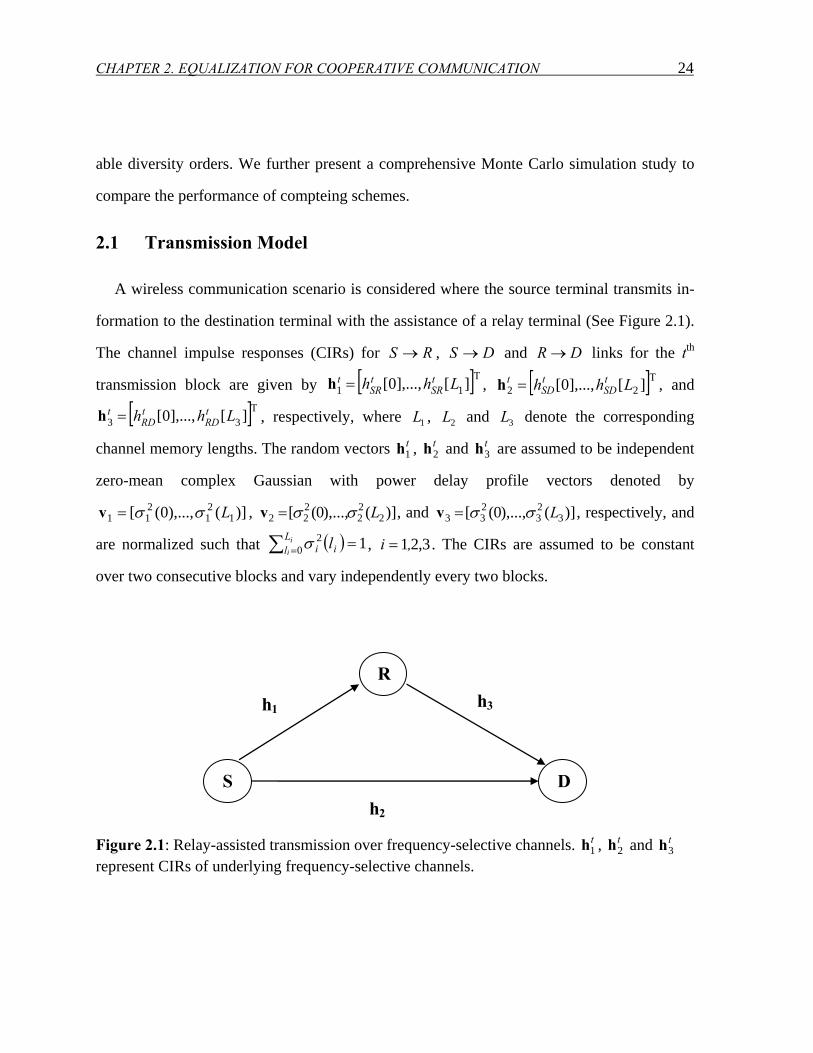
A wireless communication scenario is considered where the source terminal transmits in-
formation to the destination terminal with the assistance of a relay terminal (See Figure 2.1).
The channel impulse responses (CIRs) for RS → , DS → and DR → links for the tth
transmission block are given by [ ]Τ= ][],...,0[ 11 Lhh tSR
tSR
th , [ ]Τ= ][],...,0[ 22 Lhh tSD
tSD
th , and
[ ]Τ= ][],...,0[ 33 Lhh tRD
tRD
th , respectively, where 1L , 2L and 3L denote the corresponding
channel memory lengths. The random vectors t1h , t
2h and t3h are assumed to be independent
zero-mean complex Gaussian with power delay profile vectors denoted by
)](),...,0([ 121
211 Lσσ=v , )](),...,0([ 2
22
222 Lσσ=v , and )](),...,0([ 3
23
233 Lσσ=v , respectively, and
are normalized such that ( ) 102 =∑ =
ii
Ll ii lσ , 3,21,i = . The CIRs are assumed to be constant
over two consecutive blocks and vary independently every two blocks.
S
R
D
h1 h3
h2 Figure 2.1: Relay-assisted transmission over frequency-selective channels. t
1h , t2h and t
3h represent CIRs of underlying frequency-selective channels.
CHAPTER 2. EQUALIZATION FOR COOPERATIVE COMMUNICATION 25
As for the user cooperation protocol, we adopt Protocol III of [33]. For the DR → link,
AaF relaying is used, in which the relay terminal amplifies and re-transmits the signal re-
ceived from the source terminal in the first signaling interval. All terminals are equipped with
a single transmit and receive antenna. Any linear modulation technique such as QAM or PSK
modulation can be used.
Information symbols are first parsed to two streams of 1×V blocks tix , 2,1=i and then
multiplied by a zero-padding (ZP) matrix1 [ ]Τ×= lVV 0IΨ , of size VJ × , where
( )231 ,max LLL +=l and J is the frame length. As explained in [69], the use of zero-padding
as the precoding method in a single-carrier transmission scenario ensures that the available
multipath diversity is fully exploited. To further remove inter-block interference and make
the channel matrix circulant, a cyclic prefix (CP) with length l is added between adjacent
information blocks. Due to the adopted precoding form (i.e., zero padding), we simply insert
additional zeros at the start of the frame as CP. In a practical implementation, the block of
all-zeros at the end of the current frame can also be used as the next frame’s block of all-
zeros to be inserted at its beginning, avoiding unnecessary additional overhead.
Let SDE , SRE , and RDE represent the average energies available at the destination and
relay terminals taking into account possibly different path loss and shadowing effects in
DS → , RS → , and DR → links, respectively. The signal received at the relay terminal
during the first signaling interval is
tR
ttSR
jR E nΨxHr += 11 (2.1)
where t1H is a JJ × circulant matrix with entries )mod)((][ 1,1 Jlkt
lkt −= hH and t
Rn is the
AWGN vector with each entry having zero-mean and variance of 20N per dimension. The
1 The structure of the precoding matrix has the zero-padding form for D-TR-STBC and D-SC-STBC. For D-OFDM-STBC the precoding matrix is given by Ψ = QH , i.e., Inverse Fourier Transform (IFFT).
CHAPTER 2. EQUALIZATION FOR COOPERATIVE COMMUNICATION 26
relay terminal normalizes each entry of the received signal qtR ][r , Jq ,...,2,1= , by a factor of
( ) 02|][|E NESRq
tR +=r to ensure unit average energy and re-transmits the signal during
the second time slot. Therefore, the received signal at the destination terminal in the second
time slot is given by
tD
ttSD
tR
tRD
t EE nΨxHrHr ++= 223~ (2.2)
where tRr~ is the normalized received signal and t
Dn is the additive white Gaussian noise vec-
tor with each entry having zero-mean and variance of 20N per dimension. t2H and t
3H are
JJ × circulant matrices with entries )mod)((][ 2,2 Jlktlk
t −= hH and
)mod)((][ 3,3 Jlktlk
t −= hH , respectively. Combining (2.1) and (2.2), we obtain
tttSD
ttt
SR
SRRDt ENE
EE nΨxHΨxHHr ~22113
0++
+= , (2.3)
where we define the effective noise term as
tD
tR
SR
RDt NE
E nnHn ++
= 30
~ . (2.4)
Each entry of tn~ (conditioned on 3h ) has zero mean and a variance of
( ) ⎟⎟⎠
⎞⎜⎜⎝
⎛+
+=⎥⎦⎤
⎢⎣⎡ ∑
=
3
0
23
003
21~ L
mSR
RDn
t mNE
ENE hhn . (2.5)
The destination terminal normalizes the received signal by a factor of
( ) ( )03
02
31 NEEm SRRDLm ++∑ = h . This does not affect SNR, but simplifies the analytical
derivation [33]. After normalization, we obtain
ttttttt nΨxHΨxHHr ++= 2221131 γγ (2.6)
where tn is complex Gaussian with zero mean and variance of 20N per dimension and 1γ ,
2γ are defined as
CHAPTER 2. EQUALIZATION FOR COOPERATIVE COMMUNICATION 27
( ) 03
0
230
01
//1
)/(
NEmNE
ENE
RD
L
mSR
RDSR
∑=
++=
hγ , (2.7)
( ) 03
0
230
02
//1
)/1(
NEmNE
ENE
RD
L
mSR
SDSR
∑=
++
+=
hγ . (2.8)
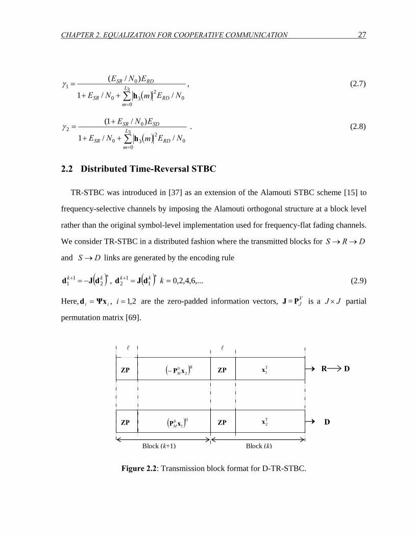
2.2 Distributed Time-Reversal STBC
TR-STBC was introduced in [37] as an extension of the Alamouti STBC scheme [15] to
frequency-selective channels by imposing the Alamouti orthogonal structure at a block level
rather than the original symbol-level implementation used for frequency-flat fading channels.
We consider TR-STBC in a distributed fashion where the transmitted blocks for DRS →→
and DS → links are generated by the encoding rule
( )∗+ −= kk2
11 dJd , ( )∗+ = kk
11
2 dJd ,...6,4,2,0=k (2.9)
Here, ii Ψxd = , 2,1=i are the zero-padded information vectors, J = VJP is a JJ × partial
permutation matrix [69].
( )Η− 20 xPM ZP ZP
ZP ZP
l l
Block (k+1) Block (k)
R D
D ( )Η10 xPM
Τ1x
Τ2x
Figure 2.2: Transmission block format for D-TR-STBC.
CHAPTER 2. EQUALIZATION FOR COOPERATIVE COMMUNICATION 28
During the kth block, the source transmits k1d to the relay terminal in the broadcasting
phase. In the relaying phase, both the relay and source terminals transmit k1d and k
2d to the
destination terminal, respectively. As for block k+1, the source transmits ( )k2dJ− to the relay
in the broadcasting phase. In the relaying phase, both the relay and source terminals transmit
( )k2dJ− and ( )∗k
1dJ to the destination terminal (c.f. Figure 2.2).
Assuming that the channel coefficients remain constant over blocks k and k+1, i.e.
iki
ki HHH == +1 , for ,3,2,1=i the received signals are given by
kkkk ndHdHHr ++= 2221131 γγ , (2.10)
( ) ( ) 11222131
1 +∗∗+ ++−= kkkk ndJHdJHHr γγ (2.11)
Taking the conjugate of 1+kr and then multiplying by the time-reversal matrix J, we have
( ) ( )∗+ΗΗΗ∗+ ++−= 11222131
1 kkkk nJdHdHHrJ γγ (2.12)
where we use the identities ΗΗ∗∗ = 1313 HHJHJH and Η∗ = 22 HJJH . Combining (2.10) and
(2.12) in matrix form yields
( ) ( ) ⎥⎦⎤
⎢⎣
⎡+⎥
⎦
⎤⎢⎣
⎡
⎥⎥⎦
⎤
⎢⎢⎣
⎡
−=⎥
⎦
⎤⎢⎣
⎡∗+ΗΗΗ∗+ 1
2
1
13122
221311 k
k
k
k
k
k
eq
nJn
dd
H
HHHHHH
rJr
44444 344444 21γγγγ
. (2.13)
Multiplying (2.13) by ( ) Η−
⎟⎠⎞
⎜⎝⎛ +⊗= eqγγ HHHHIΥ
1222
21
2312 , we observe that the data
streams are decoupled (due to orthogonality of Heq ) allowing us to write
2,1 , ,2
222
12
31 , =++= ikiout
ki
kiout ndHHHr γγ (2.14)
where kiout ,n represents the filtered noise vector which is still Gaussian with each entry hav-
ing zero-mean and a variance of 2/0N per dimension. Since the two data streams k1d and
k2d are now decoupled, each can be detected by applying standard equalization techniques
such as MMSE or MLSE (maximum likelihood sequence estimation) equalizers [70].
CHAPTER 2. EQUALIZATION FOR COOPERATIVE COMMUNICATION 29
2.2.1 Diversity Gain Analysis for D-TR-STBC
In this sub-section, we investigate the achievable diversity gain for the D-TR-STBC
scheme through the derivation of the PEP expression. First, we assume that RS → and
DS → links experience frequency-selectivity while the channel between the relay and the
destination terminals is AWGN, i.e., 1]0[3 =h . Physically, this assumption corresponds to
the case where the destination and relay terminals have a very strong line-of-sight connection
[33]. We should emphasize that this rather unrealistic assumption of static (i.e., non-fading)
DR → link is made only to simplify performance analysis and to provide a benchmark for
the general case where all underlying links experience fading.
Defining the transmitted codeword vector and the erroneously-decoded codeword vector
as x and x , respectively, the conditional PEP is given as
⎟⎟
⎠
⎞
⎜⎜
⎝
⎛=
0
2
21 2)ˆ()|ˆ,(
NdQP xx,h,hxx , (2.15)
assuming ML decoding with perfect knowledge of the CSI at the receiver side. Here, Q(.) is
the Gaussian-Q function and ( )xx ˆ,2d denotes the Euclidean distance between x and x . Ap-
plying the standard Chernoff bound to (2.15), we obtain
⎟⎟⎠
⎞⎜⎜⎝
⎛−≤
0
2
21 4)ˆ(exp)|ˆ,(
NdP xx,h,hxx . (2.16)
Noting that iii xΨd = , we can write ( )xx ˆ,2d as follows
( ) ( ) ˆˆ)ˆ,(2
222
112 ddHddHxx −+−= γγd (2.17)
where 1γ and 2γ in (2.7) and (2.8) now reduce to
00
01 //1
)/(NENE
ENE
RDSR
RDSR
++=γ , (2.18)
00
02 //1
)/1(NENE
ENE
RDSR
SDSR
+++
=γ (2.19)

CHAPTER 2. EQUALIZATION FOR COOPERATIVE COMMUNICATION 30
under the non-fading DR → link assumption. By further defining [ ])(),...,0( iiii Lhhh =Τ
and
⎥⎥⎥⎥⎥
⎦
⎤
⎢⎢⎢⎢⎢
⎣
⎡
=
−−+−−
−−
−
11
201
110
][][][
][][][][][][
iii LJLJLJ
JJ
J
i
ddd
dddddd
χ
L
MLMM
L
L
, 2,1=i (2.20)
(2.17) can be rewritten as
( ) ( ) 222
211
2 ˆˆ)ˆ,( χχhχχhxx −+−= ΤΤ γγd . (2.21)
Substituting (2.21) in (2.16) and following the steps detailed in Appendix A.1, we obtain the
final PEP form as ( ) ( )
∏∏==
+−+−
⎟⎟⎠
⎞⎜⎜⎝
⎛+⎟⎟
⎠
⎞⎜⎜⎝
⎛+≤
2
2
1
1
21
0 220 11
1
0
21
0
1
)(1
)(1
41
41)ˆ,(
L
l
L
l
LL
llNγ
Nγ
Pλλ
xx (2.22)
where iλ , 2,1=i denote the eigenvalues of the codeword difference matrix defined
by 2/12/1iiii ΩχΩΑ = with )( ii diag vΩ = and ( )( )Η−−= iiiii χχχχχ ˆˆ . In the following, we discuss
various aspects on the performance of D-TR-STBC.
Maximum Achievable Diversity for D-TR-STBC: We assume perfect power control where
DS → and DR → links are balanced and high SNRs for all underlying links, i.e.,
100 >>= NENE RDSD . It is also assumed that SNR in RS → is large enough, i.e.,
00/ NENE SDSR > . Under these assumptions, we have 1// 0201 >>= NγNγ , simplifying
(2.22) to
( )( )
( ) ( )∏∏==
++−
⎟⎟⎠
⎞⎜⎜⎝
⎛≤
2
2
1
1
21
0 220 11
2
0
1 14
ˆ,L
l
L
l
LLSD
llNE
Pλλ
xx . (2.23)
Since iΑ is full rank, the maximum achievable diversity order is given by 221 ++ LL . Un-
der the assumption of non-fading RS → link, the maximum achievable diversity order can
CHAPTER 2. EQUALIZATION FOR COOPERATIVE COMMUNICATION 31
be similarly found and is given by 223 ++ LL . If we further assume that L1=L2=L in (2.23)
(or similarly L2=L3=L for the scenario with non-fading RS → link), we obtain
( )( )
( )
2
0 1
12
0
14
ˆ, ∏=
+−
⎟⎟⎠
⎞⎜⎜⎝
⎛⎟⎟⎠
⎞⎜⎜⎝
⎛≤
L
l
LSD
lNE
Pλ
xx (2.24)
which is the PEP expression for non-distributed TR-STBC.
Existence of Error Floor: In the investigation of the maximum achievable diversity order,
we have assumed that SNR in RS → link is sufficiently large, i.e., 00/ NENE SDSR > . Now we
consider the limiting case of ∞→0/ NE SD . For this case, (2.22) takes the following form
( )( )
( ) ( )∏∏==
++−
⎟⎟⎠
⎞⎜⎜⎝
⎛≤
2
2
1
1
21
0 220 11
2
0
1 14
ˆ,L
l
L
l
LLSR
llNEP
λλxx . (2.25)
It is observed that the performance becomes independent of 0/ NE SD and is now governed
by 0/ NESR . Therefore, the performance is expected to deteriorate for low 0/ NESR resulting
in error floors, which is an inherent disadvantage of the employed Protocol III of [33]. It
should be noted that such error floors can be avoided if Protocol I of [33] is used as the user
cooperation protocol where the source-to-destination transmission is allowed within the first
signaling interval.
Effect of Power Imbalance: Now we consider the case of no power control and assume
RDSD nEE = where n is a positive number. Then, (2.22) becomes
( ) ( )
∏∏==
+−+−
⎟⎟⎟⎟⎟
⎠
⎞
⎜⎜⎜⎜⎜
⎝
⎛
++
⎟⎟⎠
⎞⎜⎜⎝
⎛+
+
⎟⎟⎟⎟⎟
⎠
⎞
⎜⎜⎜⎜⎜
⎝
⎛
+++≤
2
2
1
1
21
0 220 11
1
00
00
1
00
00
)(1
)(1
11
41
111
41
1)ˆ,(L
l
L
l
L
SDSR
SDSRL
SDSR
SDSR
llNE
nNE
NE
NE
NE
nNE
NE
NE
nP
λλxx (2.26)
For large n, we obtain
( ) ( )
∏∏==
+−+−
⎟⎟⎠
⎞⎜⎜⎝
⎛⎟⎟⎠
⎞⎜⎜⎝
⎛≤
2
2
1
1
21
0 220 11
1
0
1
0 )(1
)(1
441)ˆ,(
L
l
L
l
LSD
LSD
llNE
NE
nP
λλxx (2.27)

CHAPTER 2. EQUALIZATION FOR COOPERATIVE COMMUNICATION 32
where the performance is governed by 0/ NE SD which means that the DS → link is the
dominant link. On the other hand, for small values of n, (2.26) reduces to
( ) ( )
∏∏==
+−+−
⎟⎟⎠
⎞⎜⎜⎝
⎛⎟⎟⎠
⎞⎜⎜⎝
⎛+⎟⎟
⎠
⎞⎜⎜⎝
⎛≤
2
2
1
1
21
0 220 11
1
0
1
0 )(1
)(11
44)ˆ,(
L
l
L
l
LSR
LSR
llNEn
NE
Pλλ
xx (2.28)
where the performance is once again dominated by 0/ NESR .
Extension to fading DR → link: Now, we return our attention on the general case where all
three underlying links experience frequency-selective fading. Due to the presence of ( ) 23 mh
terms in (2.7) and (2.8), the derivation of PEP becomes analytically intractable without any
assumptions imposed on the SNR in the underlying links. However, for the asymptotic case
of 100 >>= NENE RDSD with perfect power control and sufficiently large
00/ NENE SDSR > values, the scaling factors in (2.7) and (2.8) reduce to SDEγγ == 21 .
Then, we can obtain the following PEP expressions (See Appendix A.2 for detailed steps of
the derivations)
Case 1: 13 LL >
( ) ( )( )
( )
( ) ( )∏∏=
−
=
−++−
⎟⎟⎠
⎞⎜⎜⎝
⎛+Γ+−Γ
+≤2
2
1
1
21
1
0
122
0
111
2
03
133 )()(
411
1)ˆ,(L
l
L
l
LLSDL llN
EL
LLLP λλxx (2.29)
Case 2: 31 LL >
( ) ( )( )
( )
( ) ( )∏∏=
−
=
−++−
⎟⎟⎠
⎞⎜⎜⎝
⎛+Γ+−Γ
+≤2
2
3
3
23
3
0
122
0
131
2
01
311 )()(
411
1)ˆ,(L
l
L
l
LLSDL llN
EL
LLLP λλxx (2.30)
Case 3: 31 LL =
( )( ) ( )
( )
( )∏=
−++−
−+
⎟⎟⎠
⎞⎜⎜⎝
⎛−
+Γ+
≤2
2
23
33
0
122
2
0
1
3
13 )(
41
11
)ˆ,(L
l
LLSDL
L
lN
EL
LP λxx
( ) ⎟⎟
⎠
⎞⎜⎜⎝
⎛ +−×
++
=+∑
SDi
ElLNL
lL
l
ElLN
Eel
pSD
)()1(4
)( 11
30)()1(41
11
11
11
301
13
1
λλλ (2.31)
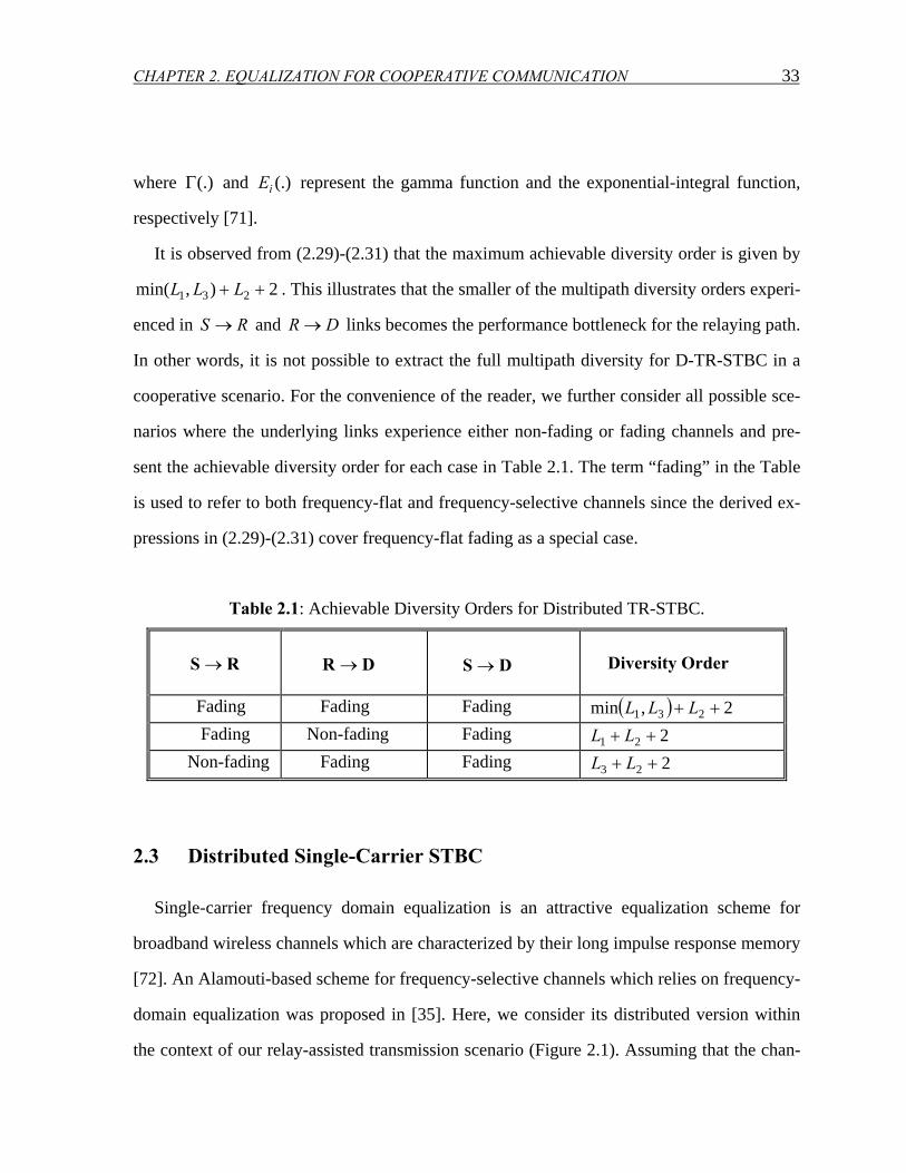
CHAPTER 2. EQUALIZATION FOR COOPERATIVE COMMUNICATION 33
where (.)Γ and (.)iE represent the gamma function and the exponential-integral function,
respectively [71].
It is observed from (2.29)-(2.31) that the maximum achievable diversity order is given by
2),min( 231 ++ LLL . This illustrates that the smaller of the multipath diversity orders experi-
enced in RS → and DR → links becomes the performance bottleneck for the relaying path.
In other words, it is not possible to extract the full multipath diversity for D-TR-STBC in a
cooperative scenario. For the convenience of the reader, we further consider all possible sce-
narios where the underlying links experience either non-fading or fading channels and pre-
sent the achievable diversity order for each case in Table 2.1. The term “fading” in the Table
is used to refer to both frequency-flat and frequency-selective channels since the derived ex-
pressions in (2.29)-(2.31) cover frequency-flat fading as a special case.
Table 2.1: Achievable Diversity Orders for Distributed TR-STBC.
Fading Fading Fading ( ) 2,min 231 ++ LLL Fading Non-fading Fading 221 ++ LL Non-fading Fading Fading 223 ++ LL
2.3 Distributed Single-Carrier STBC
Single-carrier frequency domain equalization is an attractive equalization scheme for
broadband wireless channels which are characterized by their long impulse response memory
[72]. An Alamouti-based scheme for frequency-selective channels which relies on frequency-
domain equalization was proposed in [35]. Here, we consider its distributed version within
the context of our relay-assisted transmission scenario (Figure 2.1). Assuming that the chan-
RS → DR → DS → Diversity Order
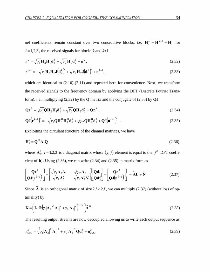
CHAPTER 2. EQUALIZATION FOR COOPERATIVE COMMUNICATION 34
nel coefficients remain constant over two consecutive blocks, i.e. iki
ki HHH == +1 for
3,2,1=i , the received signals for blocks k and k+1
kkkk ndHdHHr ++= 2221131 γγ , (2.32)
( ) ( ) 11222131
1 +∗∗+ ++−= kkkk ndJHdJHHr γγ , (2.33)
which are identical to (2.10)-(2.11) and repeated here for convenience. Next, we transform
the received signals to the frequency domain by applying the DFT (Discrete Fourier Trans-
form), i.e., multiplying (2.32) by the Q matrix and the conjugate of (2.33) by QJ
kkkk QndQHdHQHQr ++= 2221131 γγ , (2.34)
( ) ( )∗+ΗΗΗ∗+ ++−= 11222131
1 kkkk nQJdQHdHQHrQJ γγ . (2.35)
Exploiting the circulant structure of the channel matrices, we have
QΛQH ti
ti
Η= (2.36)
where 3,2,1 , =itiΛ is a diagonal matrix whose ( )jj, element is equal to the thj DFT coeffi-
cient of tih . Using (2.36), we can write (2.34) and (2.35) in matrix form as
( ) ( ) 12
1
13122
221311 ⎥
⎦
⎤⎢⎣
⎡+⎥
⎦
⎤⎢⎣
⎡
⎥⎥⎦
⎤
⎢⎢⎣
⎡
−=⎥
⎦
⎤⎢⎣
⎡∗+∗∗∗∗+ k
k
k
k
k
k
nQJQn
QdQd
ΛΛΛΛΛΛ
rQJQr
γγγγ
NUΛ ~~+= (2.37)
Since Λ~ is an orthogonal matrix of size JJ 22 × , we can multiply (2.37) (without loss of op-
timality) by
( ) Hγγ ΛΛΛΛIK ~2/1222
21
2312 ⎟
⎠⎞
⎜⎝⎛ +⊗=
−. (2.38)
The resulting output streams are now decoupled allowing us to write each output sequence as
kiout
ki
kiout ,
222
21
231, nQdΛΛΛr ++= γγ (2.39)
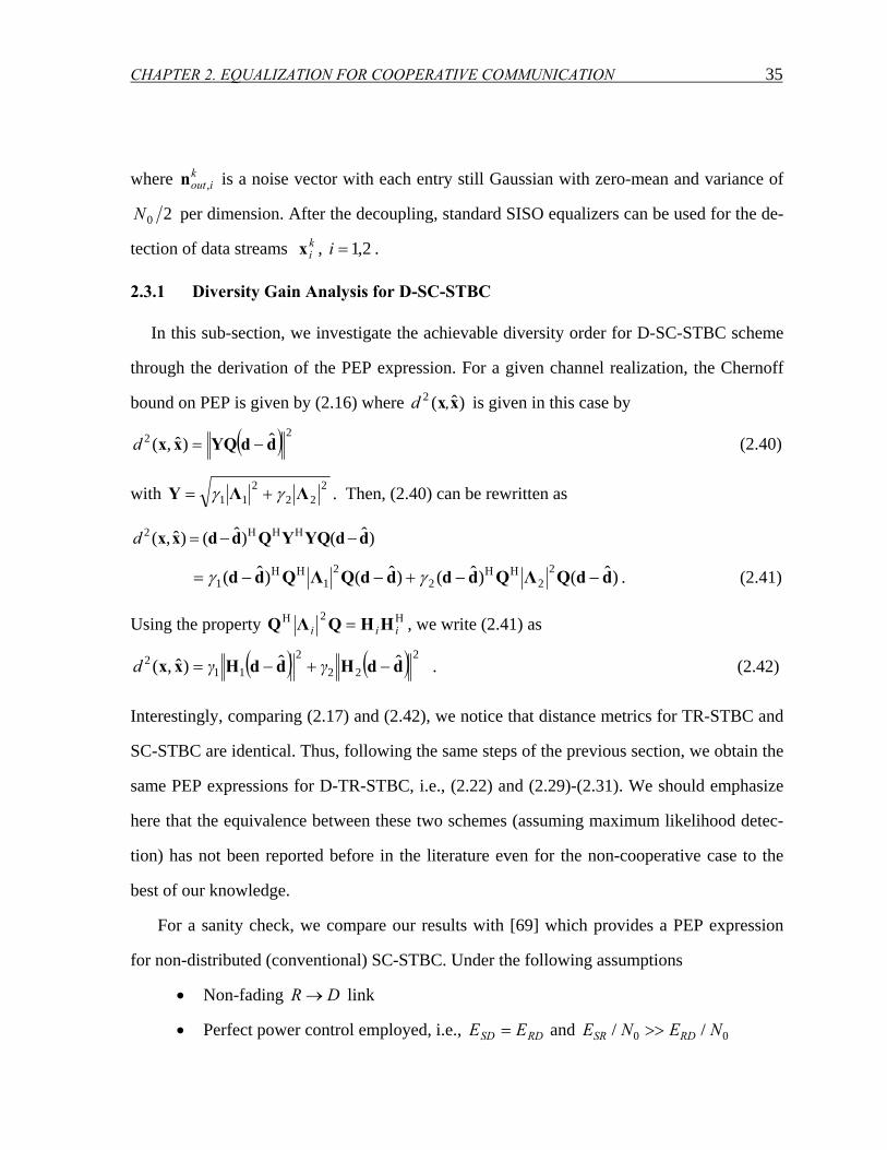
CHAPTER 2. EQUALIZATION FOR COOPERATIVE COMMUNICATION 35
where kiout ,n is a noise vector with each entry still Gaussian with zero-mean and variance of
20N per dimension. After the decoupling, standard SISO equalizers can be used for the de-
tection of data streams kix , 2,1=i .
2.3.1 Diversity Gain Analysis for D-SC-STBC
In this sub-section, we investigate the achievable diversity order for D-SC-STBC scheme
through the derivation of the PEP expression. For a given channel realization, the Chernoff
bound on PEP is given by (2.16) where )ˆ(2 xx,d is given in this case by
( ) ˆ)ˆ,(22 ddYQxx −=d (2.40)
with 222
211 ΛΛY γγ += . Then, (2.40) can be rewritten as
)ˆ()ˆ()ˆ,(2 ddYQYQddxx −−= ΗΗΗd
)ˆ()ˆ()ˆ()ˆ( 222
211 ddQΛQddddQΛQdd −−+−−= ΗΗΗΗ γγ . (2.41)
Using the property ΗΗ = iii HHQΛQ 2 , we write (2.41) as
( ) ( ) ˆˆ)ˆ,(2
222
112 ddHddHxx −+−= γγd . (2.42)
Interestingly, comparing (2.17) and (2.42), we notice that distance metrics for TR-STBC and
SC-STBC are identical. Thus, following the same steps of the previous section, we obtain the
same PEP expressions for D-TR-STBC, i.e., (2.22) and (2.29)-(2.31). We should emphasize
here that the equivalence between these two schemes (assuming maximum likelihood detec-
tion) has not been reported before in the literature even for the non-cooperative case to the
best of our knowledge.
For a sanity check, we compare our results with [69] which provides a PEP expression
for non-distributed (conventional) SC-STBC. Under the following assumptions
• Non-fading DR → link
• Perfect power control employed, i.e., RDSD EE = and 00 // NENE RDSR >>
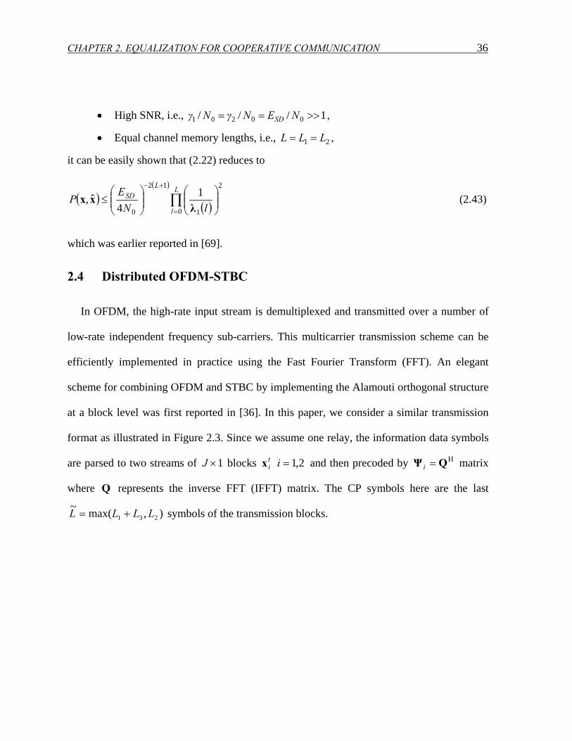
CHAPTER 2. EQUALIZATION FOR COOPERATIVE COMMUNICATION 36
• High SNR, i.e., 1/// 00201 >>== NENγNγ SD ,
• Equal channel memory lengths, i.e., 21 LLL == ,
it can be easily shown that (2.22) reduces to
( )( )
( )
2
0 1
12
0
14
ˆ, ∏=
+−
⎟⎟⎠
⎞⎜⎜⎝
⎛⎟⎟⎠
⎞⎜⎜⎝
⎛≤
L
l
LSD
lNE
Pλ
xx (2.43)
which was earlier reported in [69].
2.4 Distributed OFDM-STBC
In OFDM, the high-rate input stream is demultiplexed and transmitted over a number of
low-rate independent frequency sub-carriers. This multicarrier transmission scheme can be
efficiently implemented in practice using the Fast Fourier Transform (FFT). An elegant
scheme for combining OFDM and STBC by implementing the Alamouti orthogonal structure
at a block level was first reported in [36]. In this paper, we consider a similar transmission
format as illustrated in Figure 2.3. Since we assume one relay, the information data symbols
are parsed to two streams of 1×J blocks tix 2,1=i and then precoded by Η= QΨ i matrix
where Q represents the inverse FFT (IFFT) matrix. The CP symbols here are the last
),max(~231 LLLL += symbols of the transmission blocks.
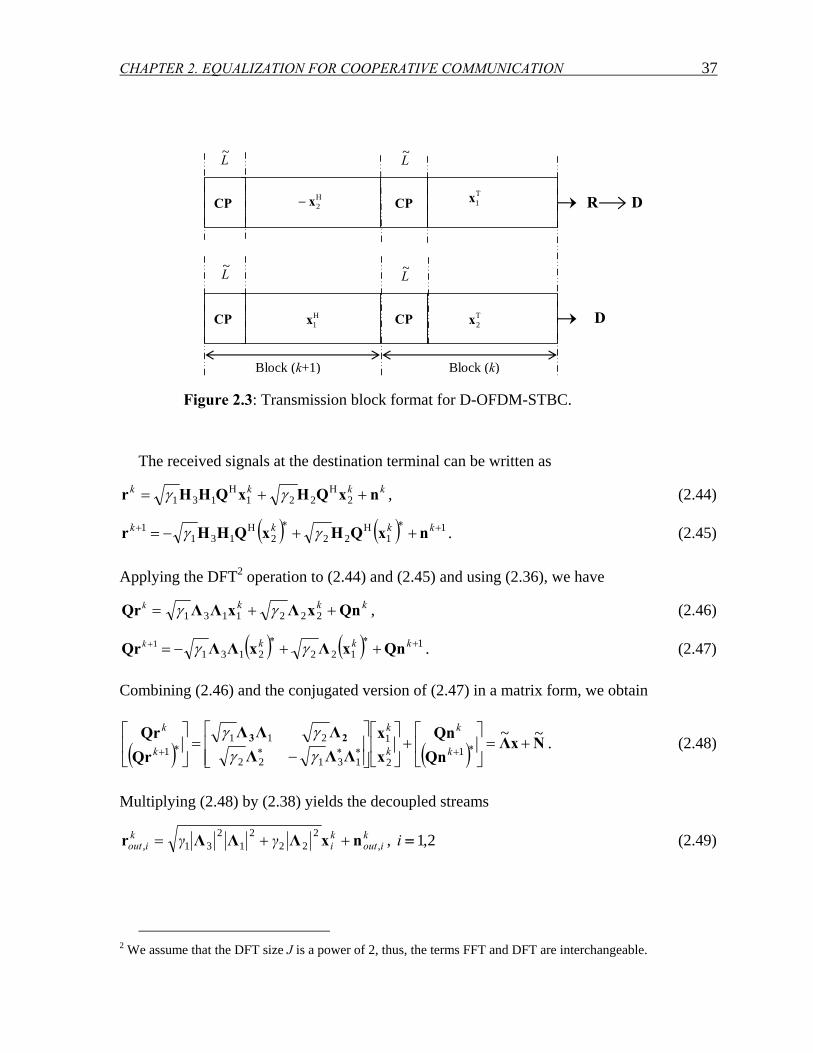
CHAPTER 2. EQUALIZATION FOR COOPERATIVE COMMUNICATION 37
Η− 2x CP CP
Η1x CP CP
L~
R D
D
Block (k+1) Block (k)
Τ1x
Τ2x
L~
L~ L~
Figure 2.3: Transmission block format for D-OFDM-STBC.
The received signals at the destination terminal can be written as
kkkk nxQHxQHHr ++= ΗΗ2221131 γγ , (2.44)
( ) ( ) 11222131
1 +∗Η∗Η+ ++−= kkkk nxQHxQHHr γγ . (2.45)
Applying the DFT2 operation to (2.44) and (2.45) and using (2.36), we have
kQr kkk QnxΛxΛΛ ++= 2221131 γγ , (2.46)
1+kQr ( ) ( ) 11222131
+∗∗++−= kkk QnxΛxΛΛ γγ . (2.47)
Combining (2.46) and the conjugated version of (2.47) in a matrix form, we obtain
( ) ( ) NxΛQn
Qnxx
ΛΛΛΛΛΛ
QrQr 23 ~~
12
1
13122
2111 +=⎥
⎦
⎤⎢⎣
⎡+⎥
⎦
⎤⎢⎣
⎡
⎥⎥⎦
⎤
⎢⎢⎣
⎡
−=⎥
⎦
⎤⎢⎣
⎡∗+∗∗∗∗+ k
k
k
k
k
k
γγγγ
. (2.48)
Multiplying (2.48) by (2.38) yields the decoupled streams
kiout
ki
kiout γγ ,
222
21
231, nxΛΛΛr ++= , 2,1=i (2.49)
2 We assume that the DFT size J is a power of 2, thus, the terms FFT and DFT are interchangeable.
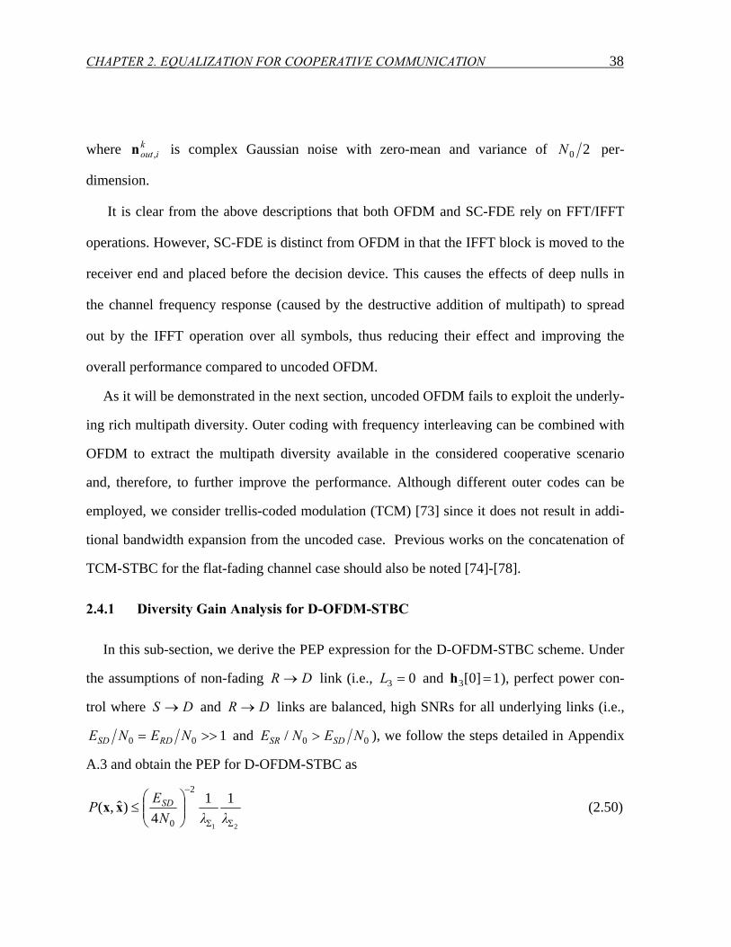
CHAPTER 2. EQUALIZATION FOR COOPERATIVE COMMUNICATION 38
where kiout ,n is complex Gaussian noise with zero-mean and variance of 20N per-
dimension.
It is clear from the above descriptions that both OFDM and SC-FDE rely on FFT/IFFT
operations. However, SC-FDE is distinct from OFDM in that the IFFT block is moved to the
receiver end and placed before the decision device. This causes the effects of deep nulls in
the channel frequency response (caused by the destructive addition of multipath) to spread
out by the IFFT operation over all symbols, thus reducing their effect and improving the
overall performance compared to uncoded OFDM.
As it will be demonstrated in the next section, uncoded OFDM fails to exploit the underly-
ing rich multipath diversity. Outer coding with frequency interleaving can be combined with
OFDM to extract the multipath diversity available in the considered cooperative scenario
and, therefore, to further improve the performance. Although different outer codes can be
employed, we consider trellis-coded modulation (TCM) [73] since it does not result in addi-
tional bandwidth expansion from the uncoded case. Previous works on the concatenation of
TCM-STBC for the flat-fading channel case should also be noted [74]-[78].
2.4.1 Diversity Gain Analysis for D-OFDM-STBC
In this sub-section, we derive the PEP expression for the D-OFDM-STBC scheme. Under
the assumptions of non-fading DR → link (i.e., 03 =L and 1]0[3 =h ), perfect power con-
trol where DS → and DR → links are balanced, high SNRs for all underlying links (i.e.,
100 >>= NENE RDSD and 00/ NENE SDSR > ), we follow the steps detailed in Appendix
A.3 and obtain the PEP for D-OFDM-STBC as
21
114
)ˆ,(2
0 ΣΣ
−
⎟⎟⎠
⎞⎜⎜⎝
⎛≤
λλNEP SDxx (2.50)
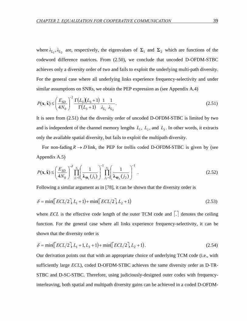
CHAPTER 2. EQUALIZATION FOR COOPERATIVE COMMUNICATION 39
where21
, ΣΣ λλ are, respectively, the eigenvalues of 1Σ and 2Σ which are functions of the
codeword difference matrices. From (2.50), we conclude that uncoded D-OFDM-STBC
achieves only a diversity order of two and fails to exploit the underlying multi-path diversity.
For the general case where all underlying links experience frequency-selectivity and under
similar assumptions on SNRs, we obtain the PEP expression as (see Appendix A.4)
( )( )( )
21
111
14
)ˆ,(3
332
0 ΣΣ
−
+Γ+Γ
⎟⎟⎠
⎞⎜⎜⎝
⎛≤
λλLLL
NEP SDxx . (2.51)
It is seen from (2.51) that the diversity order of uncoded D-OFDM-STBC is limited by two
and is independent of the channel memory lengths 1L , 2L , and 3L . In other words, it extracts
only the available spatial diversity, but fails to exploit the multipath diversity.
For non-fading DR → link, the PEP for trellis coded D-OFDM-STBC is given by (see
Appendix A.5)
∏∏=
−
=
−−
⎟⎟⎠
⎞⎜⎜⎝
⎛⎟⎟⎠
⎞⎜⎜⎝
⎛⎟⎟⎠
⎞⎜⎜⎝
⎛≤
2
2 2
1
1 1 1
1
21
1
10 )(1
)(1
4)ˆ,(
r
j
r
j
SD
jjNE
PΘΘ λλ
xxδ
. (2.52)
Following a similar argument as in [78], it can be shown that the diversity order is
⎡ ⎤( ) ⎡ ⎤( )1 ,2min1 ,2min 21 +++= LECLLECLδ (2.53)
where ECL is the effective code length of the outer TCM code and ⎡ ⎤. denotes the ceiling
function. For the general case where all links experience frequency-selectivity, it can be
shown that the diversity order is
⎡ ⎤( ) ⎡ ⎤( )1 ,2min1,1 ,2min 231 ++++= LECLLLECLδ . (2.54)
Our derivation points out that with an appropriate choice of underlying TCM code (i.e., with
sufficiently large ECL), coded D-OFDM-STBC achieves the same diversity order as D-TR-
STBC and D-SC-STBC. Therefore, using judiciously-designed outer codes with frequency-
interleaving, both spatial and multipath diversity gains can be achieved in a coded D-OFDM-
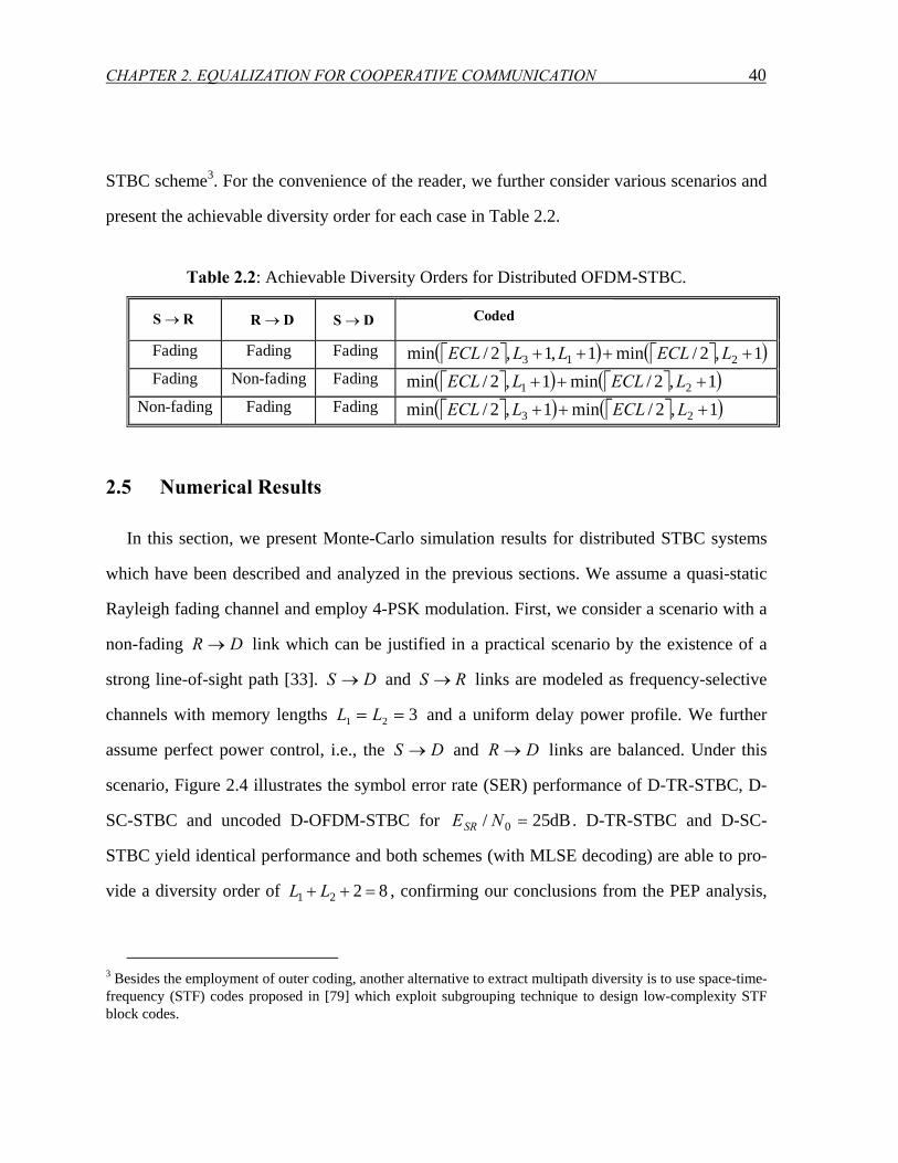
CHAPTER 2. EQUALIZATION FOR COOPERATIVE COMMUNICATION 40
STBC scheme3. For the convenience of the reader, we further consider various scenarios and
present the achievable diversity order for each case in Table 2.2.
Table 2.2: Achievable Diversity Orders for Distributed OFDM-STBC.
Fading Fading Fading ⎡ ⎤( ) ⎡ ⎤( )1,2/min1,1,2/min 213 ++++ LECLLLECLFading Non-fading Fading ⎡ ⎤( ) ⎡ ⎤( )1,2/min1,2/min 21 +++ LECLLECL
Non-fading Fading Fading ⎡ ⎤( ) ⎡ ⎤( )1,2/min1,2/min 23 +++ LECLLECL
RS → DR → DS → Coded
2.5 Numerical Results
In this section, we present Monte-Carlo simulation results for distributed STBC systems
which have been described and analyzed in the previous sections. We assume a quasi-static
Rayleigh fading channel and employ 4-PSK modulation. First, we consider a scenario with a
non-fading DR → link which can be justified in a practical scenario by the existence of a
strong line-of-sight path [33]. DS → and RS → links are modeled as frequency-selective
channels with memory lengths 321 == LL and a uniform delay power profile. We further
assume perfect power control, i.e., the DS → and DR → links are balanced. Under this
scenario, Figure 2.4 illustrates the symbol error rate (SER) performance of D-TR-STBC, D-
SC-STBC and uncoded D-OFDM-STBC for dB25/ 0 =NESR . D-TR-STBC and D-SC-
STBC yield identical performance and both schemes (with MLSE decoding) are able to pro-
vide a diversity order of 8221 =++ LL , confirming our conclusions from the PEP analysis,
3 Besides the employment of outer coding, another alternative to extract multipath diversity is to use space-time-frequency (STF) codes proposed in [79] which exploit subgrouping technique to design low-complexity STF block codes.
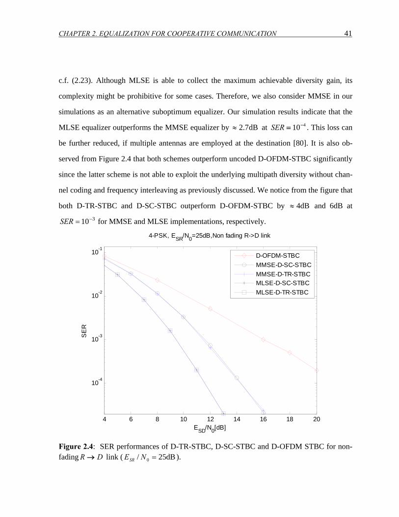
CHAPTER 2. EQUALIZATION FOR COOPERATIVE COMMUNICATION 41
c.f. (2.23). Although MLSE is able to collect the maximum achievable diversity gain, its
complexity might be prohibitive for some cases. Therefore, we also consider MMSE in our
simulations as an alternative suboptimum equalizer. Our simulation results indicate that the
MLSE equalizer outperforms the MMSE equalizer by dB7.2≈ at 410−=SER . This loss can
be further reduced, if multiple antennas are employed at the destination [80]. It is also ob-
served from Figure 2.4 that both schemes outperform uncoded D-OFDM-STBC significantly
since the latter scheme is not able to exploit the underlying multipath diversity without chan-
nel coding and frequency interleaving as previously discussed. We notice from the figure that
both D-TR-STBC and D-SC-STBC outperform D-OFDM-STBC by dB4≈ and 6dB at 310−=SER for MMSE and MLSE implementations, respectively.
4 6 8 10 12 14 16 18 20
10-4
10-3
10-2
10-1
ESD/N0[dB]
SE
R
4-PSK, ESR/N0=25dB,Non fading R->D link
D-OFDM-STBCMMSE-D-SC-STBCMMSE-D-TR-STBCMLSE-D-SC-STBCMLSE-D-TR-STBC
Figure 2.4: SER performances of D-TR-STBC, D-SC-STBC and D-OFDM STBC for non-fading DR → link ( dB25/ 0 =NESR ).
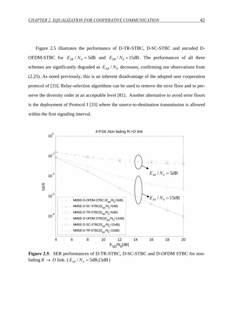
CHAPTER 2. EQUALIZATION FOR COOPERATIVE COMMUNICATION 42
Figure 2.5 illustrates the performance of D-TR-STBC, D-SC-STBC and uncoded D-
OFDM-STBC for dB5/ 0 =NESR and dB15/ 0 =NESR . The performances of all three
schemes are significantly degraded as 0/ NESR decreases, confirming our observations from
(2.25). As noted previously, this is an inherent disadvantage of the adopted user cooperation
protocol of [33]. Relay-selection algorithms can be used to remove the error floor and to pre-
serve the diversity order at an acceptable level [81]. Another alternative to avoid error floors
is the deployment of Protocol I [33] where the source-to-destination transmission is allowed
within the first signaling interval.
4 6 8 10 12 14 16 18 20
10-4
10-3
10-2
10-1
100
ESD/N0[dB]
SE
R
4-PSK,Non fading R->D link
MMSE-D-OFDM-STBC (ESR
/N0=5dB)
MMSE-D-SC-STBC(ESR
/N0=5dB)
MMSE-D-TR-STBC(ESR
/N0=5dB)
MMSE-D-OFDM-STBC(ESR
/N0=15dB)
MMSE-D-SC-STBC(ESR
/N0=15dB)
MMSE-D-TR-STBC(ESR
/N0=15dB)
Figure 2.5: SER performances of D-TR-STBC, D-SC-STBC and D-OFDM STBC for non-fading DR → link. ( dB15,dB5/ 0 =NESR )
dB5/ 0 =NESR
dB15/ 0 =NESR
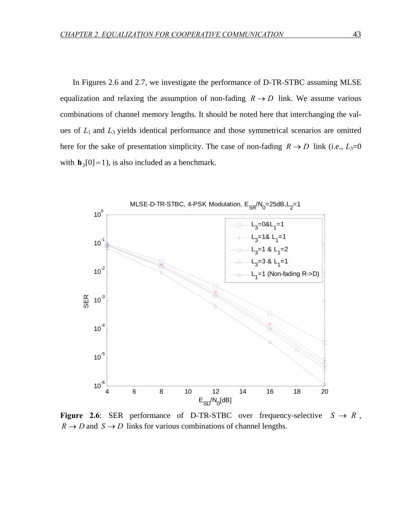
CHAPTER 2. EQUALIZATION FOR COOPERATIVE COMMUNICATION 43
In Figures 2.6 and 2.7, we investigate the performance of D-TR-STBC assuming MLSE
equalization and relaxing the assumption of non-fading DR → link. We assume various
combinations of channel memory lengths. It should be noted here that interchanging the val-
ues of L1 and L3 yields identical performance and those symmetrical scenarios are omitted
here for the sake of presentation simplicity. The case of non-fading DR → link (i.e., L3=0
with 1]0[3 =h ), is also included as a benchmark.
4 6 8 10 12 14 16 18 2010-6
10-5
10-4
10-3
10-2
10-1
100
ESD/N0[dB]
SE
R
MLSE-D-TR-STBC, 4-PSK Modulation, ESR/N0=25dB,L2=1
L3=0&L1=1
L3=1& L1=1
L3=1 & L1=2
L3=3 & L1=1
L1=1 (Non-fading R->D)
Figure 2.6: SER performance of D-TR-STBC over frequency-selective RS → ,
DR → and DS → links for various combinations of channel lengths.
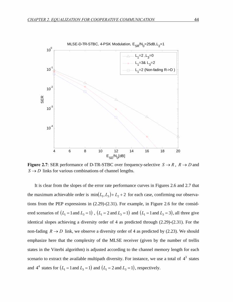
CHAPTER 2. EQUALIZATION FOR COOPERATIVE COMMUNICATION 44
4 6 8 10 12 14 16 18 20
10-4
10-3
10-2
10-1
100
ESD/N0[dB]
SE
RMLSE-D-TR-STBC, 4-PSK Modulation, ESR/N0=25dB,L2=1
L1=2 ,L3=0
L1=3& L3=2
L1=2 (Non-fading R->D )
Figure 2.7: SER performance of D-TR-STBC over frequency-selective RS → , DR → and
DS → links for various combinations of channel lengths.
It is clear from the slopes of the error rate performance curves in Figures 2.6 and 2.7 that
the maximum achievable order is ( ) 2,min 231 ++ LLL for each case, confirming our observa-
tions from the PEP expressions in (2.29)-(2.31). For example, in Figure 2.6 for the consid-
ered scenarios of ( )1 and 1 31 == LL , ( )1 and 2 31 == LL and ( ) , 3 and 1 31 == LL all three give
identical slopes achieving a diversity order of 4 as predicted through (2.29)-(2.31). For the
non-fading DR → link, we observe a diversity order of 4 as predicted by (2.23). We should
emphasize here that the complexity of the MLSE receiver (given by the number of trellis
states in the Viterbi algorithm) is adjusted according to the channel memory length for each
scenario to extract the available multipath diversity. For instance, we use a total of 34 states
and 44 states for ( )1 and 1 31 == LL and ( )1 and 2 31 == LL , respectively.
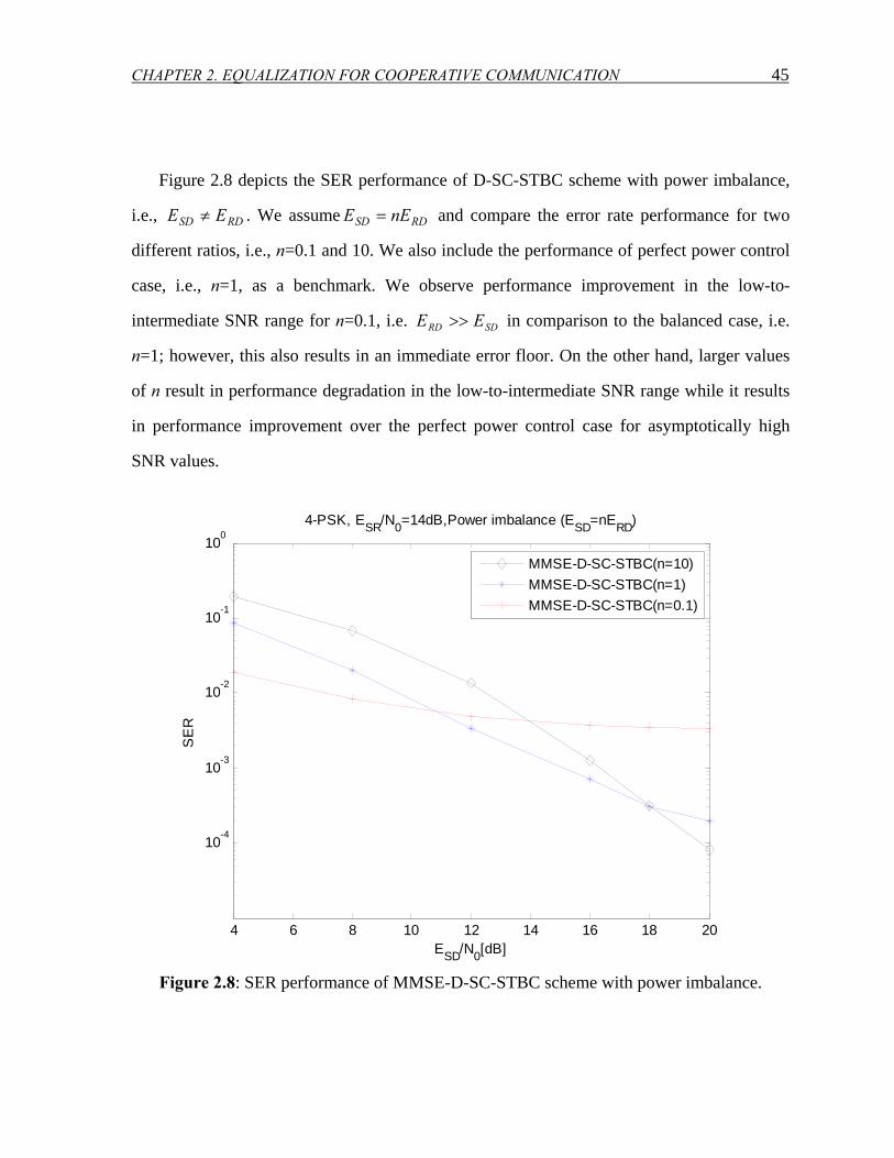
CHAPTER 2. EQUALIZATION FOR COOPERATIVE COMMUNICATION 45
Figure 2.8 depicts the SER performance of D-SC-STBC scheme with power imbalance,
i.e., RDSD EE ≠ . We assume RDSD nEE = and compare the error rate performance for two
different ratios, i.e., n=0.1 and 10. We also include the performance of perfect power control
case, i.e., n=1, as a benchmark. We observe performance improvement in the low-to-
intermediate SNR range for n=0.1, i.e. SDRD EE >> in comparison to the balanced case, i.e.
n=1; however, this also results in an immediate error floor. On the other hand, larger values
of n result in performance degradation in the low-to-intermediate SNR range while it results
in performance improvement over the perfect power control case for asymptotically high
SNR values.
4 6 8 10 12 14 16 18 20
10-4
10-3
10-2
10-1
100
ESD/N0[dB]
SE
R
4-PSK, ESR/N0=14dB,Power imbalance (ESD=nERD)
MMSE-D-SC-STBC(n=10)MMSE-D-SC-STBC(n=1)MMSE-D-SC-STBC(n=0.1)
Figure 2.8: SER performance of MMSE-D-SC-STBC scheme with power imbalance.
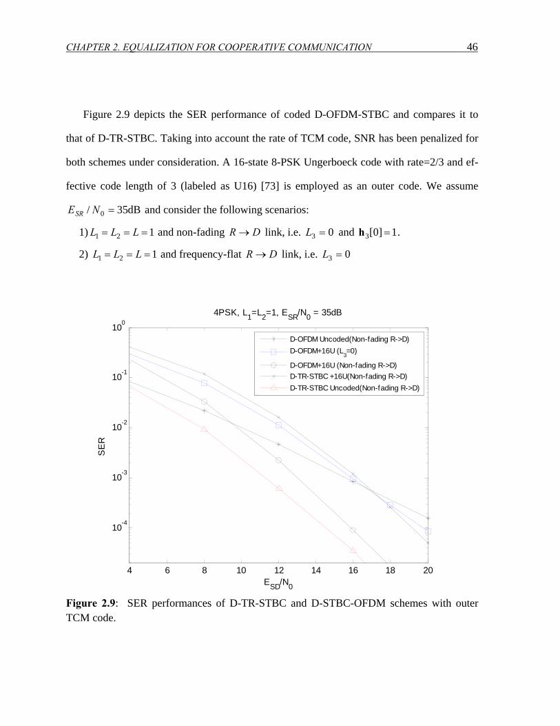
CHAPTER 2. EQUALIZATION FOR COOPERATIVE COMMUNICATION 46
Figure 2.9 depicts the SER performance of coded D-OFDM-STBC and compares it to
that of D-TR-STBC. Taking into account the rate of TCM code, SNR has been penalized for
both schemes under consideration. A 16-state 8-PSK Ungerboeck code with rate=2/3 and ef-
fective code length of 3 (labeled as U16) [73] is employed as an outer code. We assume
dB35/ 0 =NESR and consider the following scenarios:
1) 121 === LLL and non-fading DR → link, i.e. 03 =L and 1]0[3 =h .
2) 121 === LLL and frequency-flat DR → link, i.e. 03 =L
4 6 8 10 12 14 16 18 20
10-4
10-3
10-2
10-1
100
ESD/N0
SE
R
4PSK, L1=L2=1, ESR/N0 = 35dB
D-OFDM Uncoded(Non-fading R->D)D-OFDM+16U (L
3=0)
D-OFDM+16U (Non-fading R->D)D-TR-STBC +16U(Non-fading R->D)D-TR-STBC Uncoded(Non-fading R->D)
Figure 2.9: SER performances of D-TR-STBC and D-STBC-OFDM schemes with outer TCM code.
CHAPTER 2. EQUALIZATION FOR COOPERATIVE COMMUNICATION 47
As Figure 2.9 clearly demonstrates, coded D-OFDM-STBC has comparable performance
to D-TR-STBC achieving the same diversity order. Specifically, D-OFDM-STBC achieves a
diversity order of 4, as predicted by (2.53), i.e., ⎡ ⎤( ) 4 21 ,22/ min2 ==+=× LECL . For
the second scenario, we observe a diversity order of 3 confirming (2.54), i.e.,
⎡ ⎤( )1,2 ,22min =ECL ⎡ ⎤( ) 32 ,22min ==+ ECL . It is also interesting to note that the per-
formance of the uncoded D-TR-STBC outperforms its coded version. This is a result of the
fact that we assume separate decoding and equalization in our implementation. A similar ob-
servation has been reported in [82], [83] in the context of conventional TCM systems.
CHAPTER 2. EQUALIZATION FOR COOPERATIVE COMMUNICATION 48
Appendix A
This Appendix presents the derivations of PEP expressions for D-TR-STBC, uncoded D-
OFDM-STBC and TCM-D-OFDM-STBC. In the following, we drop the indices (k,i) for no-
tational brevity.
Appendix A.1 Derivation of Eq. (2.22)
In this Appendix, we derive the PEP expression for D-TR-STBC scheme for non-fading
DR → link and frequency-selective RS → and DS → links. Defining the transmitted
codeword vector and erroneously decoded codeword vector as x and x , respectively, the
Chernoff bound on PEP is given as
⎟⎟⎠
⎞⎜⎜⎝
⎛−≤
0
2
21 4)ˆ(exp)|ˆ,(
NdP xx,h,hxx (2.55)
where ( )xx ˆ,2d is earlier defined by (2.21) and repeated below for the reader’s convenience
( ) ( ) 222
211
2 ˆˆ)ˆ,( χχhχχhxx −+−= ΤΤ γγd .
By introducing ( )( )Η−−= iiiii χχχχχ ˆˆ with dimensions of )1()1( +×+ ii LL , (2.21) can be written
as
( ) ( )ΗΤΤΗΤΤ += 222211112 )ˆ,( hχhhχhxx γγd . (2.56)
Further defining )( ii diag vΩ = , iii hΩµ 2/1−= , and 2/12/1iiii ΩχΩΑ = 2,1=i , we obtain
( ) ( )ΗΤΤΗΤΤ += 222211112 )ˆ,( µΑµµΑµxx γγd . (2.57)
where iΑ , 2,1=i , are full rank due to zero padding [69]. Since iΑ is Hermitian, there exists
a unitary matrix iAU such that ii ii∆UAU AA =Η where i∆ is a real diagonal matrix of size
CHAPTER 2. EQUALIZATION FOR COOPERATIVE COMMUNICATION 49
( )( )11 ++ ii LL with non-negative entries. Noting that the diagonal elements of i∆ are the ei-
genvalues of iΑ , (2.57) can be written as
ΗΗ += 222211112 )ˆ,( β∆ββ∆βxx γd γ (2.58)
where 2,1 , == Τ iiii AUµβ is a zero-mean complex Gaussian vector with unit variance. Thus,
we can express (2.58) as
∑∑==
+=2
2
1
1 0
222222
0
211111
2 )()()()()ˆ,( L
l
L
lllγllγd βλβλxx (2.59)
where )( ii lλ denotes the thil eigenvalue of i∆ . Substituting (2.59) in (2.55) and averaging the
resulting expression with respect to ( )11 lβ and ( )22 lβ which are Rayleigh distributed, we
obtain the final PEP expression as
∏∏=
−
=
−
⎟⎟⎠
⎞⎜⎜⎝
⎛+⎟⎟
⎠
⎞⎜⎜⎝
⎛+≤
2
2
1
1 0
1
220
2
0
1
110
1 )(4
1)(4
1)ˆ,(L
l
L
ll
Nl
NP λλxx γγ . (2.60)
Appendix A.2 Derivation of Eqs. (2.29)-(2.31)
In this Appendix, we derive the PEP expression for the D-TR-STBC scheme assuming
frequency-selective channels in RS → , DS → and DR → links. The Chernoff bound on
PEP is given as
⎟⎟⎠
⎞⎜⎜⎝
⎛−≤
0
2
321 4)ˆ(exp),|ˆ,(
NdP xx,hh,hxx . (2.61)
The Euclidean distance between x and x can be written as
( ) ( ) ˆˆ)ˆ,(2
222
1312 ddHddHHxx −+−= γγd (2.62)
CHAPTER 2. EQUALIZATION FOR COOPERATIVE COMMUNICATION 50
where SDEγγ == 21 . To simplify analysis, (2.62) can be approximated4 as
( ) ( ) 222
21
23
12 ˆˆ)ˆ,( ddHddHHxx −+−≈ γγJ
d
( ) ( ) 222
23
21
1 ˆˆ ddHddHH −+−≈ γγJ
. (2.63)
where J is the frame length. Noting that 22
0)(∑
== i
i
Ll iii lJ hH , i=1,3 , we can further write
(2.63) as
( ) ( ) ( ) 222
21
03
2
3312 ˆˆ)ˆ,(
3
ddHddHhxx −+−≈ ∑=
γγL
lld
( ) ( ) ( ) 222
23
0
2111 ˆˆ
1
1
ddHddHh −+−≈ ∑=
γγL
ll . (2.64)
Following similar steps in Appendix A.1, we can write (2.64) as follows
∑∑∑==
+≈=
2
2
1
1
3
03 0
222222
0
21111
2331
2 )()()()()()ˆ,( L
l
L
l
Lllγlllγd
l
βλβλhxx (2.65)
∑∑∑==
+≈=
2
2
3
3
1
01 0
222222
0
23131
2111 )()()()()(
L
l
L
l
Lllγlllγ
l
βλβλh (2.66)
where )( ii lλ , i=1,2 denote the thil eigenvalue of codeword difference matrixes and iβ are
zero-mean complex Gaussian vectors with unit variance. In the following, we will derive the
PEP expression under three different scenarios:
Case 1: 13 LL >
First, we define the random variables ∑ == 22 0
222222 )()(L
l llY βλ and 211 XXY = with
∑ == 33 0
2331 )(L
l lX h and ∑ == 11 0
211112 )()(L
l llX βλ . Substituting (2.65) in (2.61) and averag-
ing the resulting expression with respect to 1Y and 2Y , we obtain
4 Through a Monte-Carlo simulation experiment, we have observed that the mean square error (MSE) difference between (2.62) and (2.63) is only ~0.3 at =0/NESD 4dB. The approximate expression converges to the exact one as early as =0/NESD 6dB. Therefore, this approximation can be used safely for any practical purpose.
CHAPTER 2. EQUALIZATION FOR COOPERATIVE COMMUNICATION 51
⎥⎥⎦
⎤
⎢⎢⎣
⎡⎟⎟⎠
⎞⎜⎜⎝
⎛−
⎥⎥⎦
⎤
⎢⎢⎣
⎡⎟⎟⎠
⎞⎜⎜⎝
⎛−≤ 2
01
0 4exp
4exp)ˆ,(
21Y
NE
EYN
EEP SD
YSD
Yxx
( ) ( )0
2
0
14
4
N
EjYN
EjY SDSD −=−=Φ×Φ=
ωωωω (2.67)
where ( )ω1YΦ and ( )ω2YΦ are the characteristic functions of Y1 and Y2 respectively. Since
the entries of 2β are Rayleigh distributed, ( )ω2YΦ is readily found as [84]
∏=
−
−= ⎟⎟⎠
⎞⎜⎜⎝
⎛+=Φ
2
20
20
1
204
)(
41) (
L
l
SD
NE
jY lN
ESD λ
ωω . (2.68)
( )ω1YΦ can be evaluated as [85]
∫∞
Φ=Φ0
1111 ) ()()(21
dxxxf XXY ωω (2.69)
where 0 ),( 111≥xxf X is the probability density function (pdf) of 1X and ) ( 12
xX ωΦ is the
characteristic function of 2X . In our case, 3h are modeled as zero-mean complex Gaussian
random variables with variance ( )12/1 3 +L per-dimension (i.e., uniform power profile).
Therefore, 1X is a chi-squared random variable with ( )12 3 +L degrees of freedom with the
following pdf [86],
( )( )
( )11
3
13
1313
3
1 11
)( +−+
+Γ+
= LxLL
X exL
Lxf . (2.70)
Substituting (2.70) in (2.69) and also noting ( )∏ = −=Φ 112 0 111 )( 11) ( LlX lxjx λωω [84], (2.69) can
be written as
( )0
14
N
EjY SD−=Φ
ωω
( )( )
( )
( )( )
∫∏
∏∞ −
=
−+−+
⎟⎟⎠
⎞⎜⎜⎝
⎛+
⎟⎟⎠
⎞⎜⎜⎝
⎛+Γ
+=
+
01
1011
1
0
111
1
03
13
1
1
13131
1
13
4)(
1)(
411
dxx
NEl
exl
NE
LL
L
l SD
xLL
l
LSD
L L
λ
λ (2.71)
Assuming high SNR, i.e., 04NESD >>1, (2.71) yields

CHAPTER 2. EQUALIZATION FOR COOPERATIVE COMMUNICATION 52
( ) ( )( )
( )
( ) ( )∫∏∞
+−−
=
−+−+
−= ⎟⎟⎠
⎞⎜⎜⎝
⎛+Γ
+=Φ
01
11
0
111
1
03
13
4
31131
1
13
0
1)(
411
dxexlN
EL
L LxLLL
l
LSD
L
NEjY SD λ
ωω . (2.72)
Using the integral form given by [71, p.382, 3.351.3], we obtain
( ) ( ) ( )( )
( )
( )∏=
−+−
−= ⎟⎟⎠
⎞⎜⎜⎝
⎛+Γ+−Γ
+=Φ1
1
1
1
0
10
111
1
03
133
4
)(41
11
L
l
LSDL
NEjY l
NE
LLL
LSD λω
ω . (2.73)
Substituting (2.73) and (2.68) in (2.67), we find the final PEP expression as
( ) ( )( )
( )
( ) ( )∏∏=
−
=
−++−
⎟⎟⎠
⎞⎜⎜⎝
⎛+Γ+−Γ
+≤2
2
1
1
21
1
0
122
0
111
2
03
133 )()(
411
1)ˆ,(L
l
L
l
LLSDL llN
EL
LLLP λλxx (2.74)
Case 2: 31 LL >
Using (2.66) and noting that this case is similar to Case 1 with 1L and 3L now interchanged,
the PEP expression is found as
( ) ( )( )
( )
( ) ( )∏∏=
−
=
−++−
⎟⎟⎠
⎞⎜⎜⎝
⎛+Γ+−Γ
+≤2
2
3
3
23
3
0
122
0
131
2
01
311 )()(
4111)ˆ,(
L
l
L
l
LLSDL llN
EL
LLLP λλxx . (2.75)
Case 3: 31 LL =
Following the same argument in Case 1 and using partial fraction expansion, (2.71) can be
rewritten as
( ) ( )( )
( )
∫∑∞ +−+
=
+
−=
⎟⎟⎠
⎞⎜⎜⎝
⎛+
+Γ+
=Φ0
1
1011
11
1
1 0113
13
4
4)(
14)(11 3131
1
13
0
1dx
xNEl
exNEl
pL
L
SD
LxLL
l SD
lL
NEjY SD
λλω
ω (2.76)
where ( ) ( ) ( )( )∏ ≠= −= 1
11 ,0 11111L
llll lllp λλλ . Using the integral form given by [71, p.338,
3.353.5.7] and after some mathematical manipulation, we obtain
CHAPTER 2. EQUALIZATION FOR COOPERATIVE COMMUNICATION 53
( ) ( )( ) ( ) ( ) ( )
( ) ⎟⎟⎠
⎞⎜⎜⎝
⎛ +−−
+Γ+
=Φ++
=+
+−−+
−= ∑SD
iEl
LNL
lL
lLSD
LL
NE
jY ElLN
Eel
pNE
LL
SDSD )(
)1(4)(
411
1
11
30)()1(41
11
11
10
1
3
13
4
11
301
13
1333
0
1 λλλ
ωω
( )( ) ( ) ( ) ( )
( )( )∑∑
+
=
−+−−+
=
−−+
+−−+Γ
++
1
1
)1(01
1113
3
13
1
1
3
3
13
33
4)(
11!11
1 L
l
kLSDkL
lL
k
kkLL
NEl
pLk
LL
λ (2.77)
where (.)Γ and (.)iE represent the gamma function and the exponential-integral function,
respectively [71]. Using the fact ( ) )1 ( 0 11
1 111
1 1 LrlpLl
rl ≤≤=∑ +
= λ and noting that 31 LL = , the
second term in (2.77) becomes zero. Substituting (2.77) and (2.68) in (2.67) and assuming
high SNR, we find the PEP expression given as
( )( ) ( )
( )
( )( ) ⎟⎟
⎠
⎞⎜⎜⎝
⎛ +−⎟⎟
⎠
⎞⎜⎜⎝
⎛−
+Γ+
≤++
=+
=
−++−
−+
∑∏SD
iEl
LNL
lL
lL
l
LLSDL
L
ElLN
Eel
pl
NE
LL
P SD
)()1(4
)()(
41
11
)ˆ,(11
30)()1(41
11
110
122
2
0
1
3
13 11
301
13
12
2
23
33
λλλxx λ
(2.78)
Appendix A.3 Derivation of Eq. (2.50)
In this Appendix, we derive the PEP expression for the D-OFDM-STBC scheme assuming
a non-fading DR → link. For this scheme, the distance metric )ˆ(2 xx,d is given by
( ) ( ) 2222
2111
2 )ˆ(diag)ˆ(diag)ˆ( hfxxhfxxxx −+−= γγ,d , (2.79)
where we define )/)1)(1(2exp( Jqpji −−−= πf , Jp ,...1= , 1,...1 += iLq . This can be fur-
ther simplified as
222211112 )ˆ,( εΣεεΣεxx ΗΗ += γγd (2.80)
where ( ) ( ) iiiiiii UΩfxxfxxΩUΣ 2/12/1 )ˆ(diag)ˆ(diag −−= ΗΗ and iiii hΩUε 2/1−Η= , 2,1=i and
iU is a unitary matrix. Note that iΣ is a rank-one Hermitian matrix of size ( )( )11 ++ ii LL .
Substituting (2.80) in (2.55), we follow similar steps as in Appendix A.1 to obtain the final
form for PEP as
CHAPTER 2. EQUALIZATION FOR COOPERATIVE COMMUNICATION 54
21
114
)ˆ,(2
0 ΣΣ
−
⎟⎟⎠
⎞⎜⎜⎝
⎛≤
λλNEP SDxx (2.81)
where 21
, ΣΣ λλ are the eigenvalues of 1Σ and 2Σ , respectively.
Appendix A.4 Derivation of Eq. (2.51)
In this Appendix, we derive the PEP expression for the D-OFDM-STBC scheme given
that all underlying links are frequency-selective. For this scheme, the distance metric
)ˆ(2 xx,d is given by
( ) ( ) 2222
233111
2 )ˆ(diag)ˆ(diag)ˆ( hfxxhfhfxxxx −+−= γγ,d . (2.82)
Using similar arguments of Appendix A.2, we can write the distance metric as
22221110
2331
2 3
3
)( )ˆ,( εΣεεΣεhxx ΗΗ
=+≈ ∑ γγ
L
lld (2.83)
Substituting (2.83) in (2.61) and following the steps in detailed in AppendixA.2, we obtain
( )( )( )
21
111
14
)ˆ,(3
332
0 ΣΣ
−
+Γ+Γ
⎟⎟⎠
⎞⎜⎜⎝
⎛≤
λλLLL
NEP SDxx (2.84)
where 21 , ΣΣ λλ are the eigenvalues of 1Σ and 2Σ , respectively.
Appendix A.5 Derivation of Eq. (2.52)
In this Appendix, we derive the PEP expression for trellis-coded D-OFDM-STBC scheme.
Instead of the uncoded data in the original D-OFDM-STBC scheme, the TCM encoder out-
puts are interleaved and then precoded by the IFFT matrix ΗQ . Denote
[ ]]1[]1[].......1[]1[]0[]0[ 212121 −−= JxJxxxxxx as the output of the TCM encoder. Further-
more, let the transmitted symbols be [ ]]1[]......1[]0[ 1111 −= Jxxxx and
[ ]]1[]......1[]0[ 2222 −= Jxxxx . For this scheme, assuming non-fading DR → link, we have
222211112 )ˆ,( εΘεεΘεxx ΗΗ += γγd (2.85)
CHAPTER 2. EQUALIZATION FOR COOPERATIVE COMMUNICATION 55
where iiiiiii UΩPffΩUΘ 2/12/1 ΗΗ= , ( )222
211 ˆˆ xxxxP −+−= diag . Replacing (2.85) in (2.55)
and following similar steps as in Appendix A.1, we obtain the final PEP as
( ) ( )∏∏=
−
=
−−
⎟⎟⎠
⎞⎜⎜⎝
⎛≤
2
22
1
11
1
12
1
11
0)()(
4)ˆ,(
r
j
r
j
SD jjN
EP ΘΘ λλxx
δ
(2.86)
where δ is defined as 21 rr +=δ . Here, ir and )( ijiΘλ , ii rj ,...,1= for 2,1=i are the rank
and the eigenvalues of the matrix iΘ , respectively.
56
Chapter 3 Non-Coherent and Mismatched-Coherent
Detection for Cooperative Communication
Introduction
The majority of the current works on cooperative diversity build upon a coherent scenario
where perfect CSI is available at the destination terminal. In practice, the fading channel co-
efficients are first estimated and then used in the detection process. Relay terminals operating
in DaF mode also require CSI in the source-to-relay link for the decoding process. For AaF
relaying, the knowledge of CSI at relay terminal is essential for appropriately scaling the re-
ceived signal to satisfy relay power constraints. The quality of channel estimates thus affects
the overall performance of cooperative transmission and might become a performance limit-
ing factor.
3.1 Transmission Model
We consider the wireless communication system scenario illustrated in Figure 3.1. As for
the user cooperation protocol, we adopt Protocol I of [33] and assume that the relay operates
in AaF mode. Perfect synchronization is assumed among the cooperating terminals.
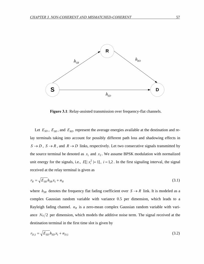
CHAPTER 3. NON-COHERENT AND MISMATCHED-COHERENT 57
S
R
D
SRh
SDh
RDh
Figure 3.1: Relay-assisted transmission over frequency-flat channels.
Let SDE , SRE , and RDE represent the average energies available at the destination and re-
lay terminals taking into account for possibly different path loss and shadowing effects in
DS → , RS → , and DR → links, respectively. Let two consecutive signals transmitted by
the source terminal be denoted as 1x and 2x . We assume BPSK modulation with normalized
unit energy for the signals, i.e., ]1|[| 2 =ixE , 2,1=i . In the first signaling interval, the signal
received at the relay terminal is given as
RSRSRR nxhEr += 1 (3.1)
where SRh denotes the frequency flat fading coefficient over RS → link. It is modeled as a
complex Gaussian random variable with variance 0.5 per dimension, which leads to a
Rayleigh fading channel. Rn is a zero-mean complex Gaussian random variable with vari-
ance 20N per dimension, which models the additive noise term. The signal received at the
destination terminal in the first time slot is given by
1,11, DSDSDD nxhEr += (3.2)

CHAPTER 3. NON-COHERENT AND MISMATCHED-COHERENT 58
where SDh denotes the complex fading coefficient over DS → link modeled as a complex
Gaussian random variable with variance 0.5 per dimension and 1,Dn is the additive noise
term modeled as a zero-mean complex Gaussian random variable with variance 20N per
dimension. The relay terminal normalizes the received signal Rr by a factor of ]||[ 2RrE to
ensure the unity of average energy and re-transmits the signal during the second time slot.
Therefore, the received signal at the destination terminal in the second time slot is given as
2,222,]|[|
DSDSDR
RRDRDD nxhE
rE
rhEr ++= (3.3)
where 2,Dn is the additive noise term modeled as a zero-mean complex Gaussian random
variable with variance 20N per dimension. RDh denotes the complex fading coefficient over
the DR → link and is modeled as a complex Gaussian random variable with variance 0.5 per
dimension. Replacing (3.1) and the normalization factor 02 ]|[| NErE SRR += in (3.3), we
obtain
nxhExhhNE
EEr SDSDSRRDSR
SRRDD
~21
02, ++
+= (3.4)
with
2,0
~DRRD
SR
RD nnhNE
En ++
= . (3.5)
In (3.5), n~ (conditioned on RDh ) is zero-mean complex Gaussian with variance of
⎟⎟
⎠
⎞
⎜⎜
⎝
⎛
++=⎥⎦
⎤⎢⎣⎡
0
2
02 1~
NEhE
NhnESR
RDRDRD . (3.6)
We can rewrite the received signal normalizing (3.4) with (3.6) as
nxhExhhEr SDSDSRRDRDD ++= 22112, ββ (3.7)
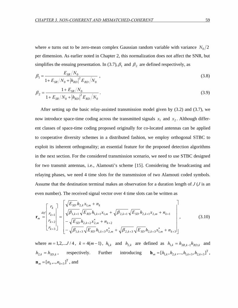
CHAPTER 3. NON-COHERENT AND MISMATCHED-COHERENT 59
where n turns out to be zero-mean complex Gaussian random variable with variance 20N
per dimension. As earlier noted in Chapter 2, this normalization does not affect the SNR, but
simplifies the ensuing presentation. In (3.7), 1β and 2β are defined respectively, as
02
0
01
1 NEhNENE
RDRDSR
SR
++=β , (3.8)
02
0
02
11
NEhNENE
RDRDSR
SR
++
+=β . (3.9)
After setting up the basic relay-assisted transmission model given by (3.2) and (3.7), we
now introduce space-time coding across the transmitted signals 1x and 2x . Although differ-
ent classes of space-time coding proposed originally for co-located antennas can be applied
to cooperative diversity schemes in a distributed fashion, we employ orthogonal STBC to
exploit its inherent orthogonality; an essential feature for the proposed detection algorithms
in the next section. For the considered transmission scenario, we need to use STBC designed
for two transmit antennas, i.e., Alamouti’s scheme [15]. Considering the broadcasting and
relaying phases, we need 4 time slots for the transmission of two Alamouti coded symbols.
Assume that the destination terminal makes an observation for a duration length of J (J is an
even number). The received signal vector over 4 time slots can be written as
⎥⎥⎥⎥⎥⎥
⎦
⎤
⎢⎢⎢⎢⎢⎢
⎣
⎡
++−
+−
++
+
=
⎥⎥⎥⎥
⎦
⎤
⎢⎢⎢⎢
⎣
⎡
=
+∗
++∗
++
+∗
+
+++++
+
+
+
3,13,23,2,23,13,1
2,22,2
1,21,21,2,11,11,1
,1,2
3
2
1
kmkSDkmkRDk
kmkSD
kmkSDkmkRDk
kmkSD
k
k
k
kdef
m
nxhExhE
nxhE
nxhExhE
nxhE
rrrr
ββ
ββr , (3.10)
where 4/,...2,1 Jm = , )1(4 −= mk , kh ,1 and kh ,2 are defined as kRDkSRk hhh ,1,,1 −= and
kSDk hh ,,2 = , respectively. Further introducing Τ++= ],,...,,[ 3,23,1,2,1 kkkkm hhhhh ,
Τ+= ],..,[ 3kkm nnn , and
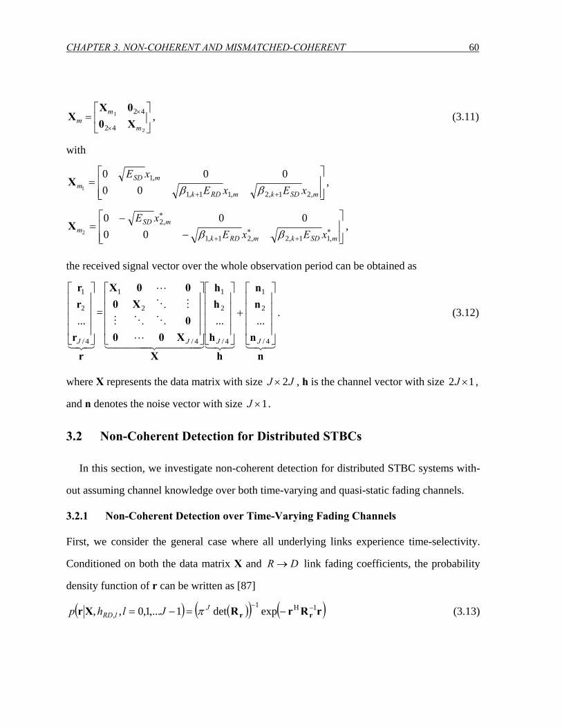
CHAPTER 3. NON-COHERENT AND MISMATCHED-COHERENT 60
⎥⎦
⎤⎢⎣
⎡=
×
×
2
1
42
42
m
mm X0
0XX , (3.11)
with
⎥⎥⎦
⎤
⎢⎢⎣
⎡=
++ mSDkmRDk
mSDm xExE
xE
,21,2,11,1
,1
00000
1 ββX ,
⎥⎥⎦
⎤
⎢⎢⎣
⎡
−−
= ∗+
∗+
∗
mSDkmRDk
mSDm xExE
xE
,11,2,21,1
,2
00000
2 ββX ,
the received signal vector over the whole observation period can be obtained as
321r
r
rr
⎥⎥⎥⎥
⎦
⎤
⎢⎢⎢⎢
⎣
⎡
4/
2
1
...
J
=
3213214444 34444 21L
OOM
MO
L
n
n
nn
h
h
hh
X
X000
X000X
⎥⎥⎥⎥
⎦
⎤
⎢⎢⎢⎢
⎣
⎡
+
⎥⎥⎥⎥
⎦
⎤
⎢⎢⎢⎢
⎣
⎡
⎥⎥⎥⎥
⎦
⎤
⎢⎢⎢⎢
⎣
⎡
4/
2
1
4/
2
1
4/
2
1
......
JJJ
. (3.12)
where X represents the data matrix with size JJ 2× , h is the channel vector with size 12 ×J ,
and n denotes the noise vector with size 1×J .
3.2 Non-Coherent Detection for Distributed STBCs
In this section, we investigate non-coherent detection for distributed STBC systems with-
out assuming channel knowledge over both time-varying and quasi-static fading channels.
3.2.1 Non-Coherent Detection over Time-Varying Fading Channels
First, we consider the general case where all underlying links experience time-selectivity.
Conditioned on both the data matrix X and DR → link fading coefficients, the probability
density function of r can be written as [87]
( ) ( )( ) ( )rRrRXr rr11
, expdet1,...1,0,, −Η−−=−= J
lRD Jlhp π (3.13)
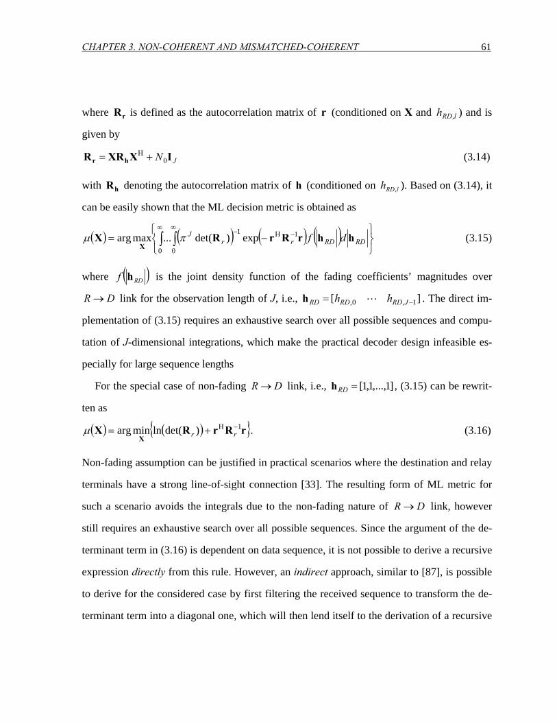
CHAPTER 3. NON-COHERENT AND MISMATCHED-COHERENT 61
where rR is defined as the autocorrelation matrix of r (conditioned on X and lRDh , ) and is
given by
JN IXXRR hr 0+= Η (3.14)
with hR denoting the autocorrelation matrix of h (conditioned on lRDh , ). Based on (3.14), it
can be easily shown that the ML decision metric is obtained as
( ) ( ) ( ) ( )⎭⎬⎫
⎩⎨⎧
−= ∫ ∫∞ ∞
−Η−
0 0
11exp)det(...maxarg RDRDrr
J df hhrRrRXX
πµ (3.15)
where ( )RDf h is the joint density function of the fading coefficients’ magnitudes over
DR → link for the observation length of J, i.e., ][ 1,0, −= JRDRDRD hh Lh . The direct im-
plementation of (3.15) requires an exhaustive search over all possible sequences and compu-
tation of J-dimensional integrations, which make the practical decoder design infeasible es-
pecially for large sequence lengths
For the special case of non-fading DR → link, i.e., ]1,...,1,1[=RDh , (3.15) can be rewrit-
ten as
( ) ( ) rRrRXX
1)det(lnminarg −Η+= rrµ . (3.16)
Non-fading assumption can be justified in practical scenarios where the destination and relay
terminals have a strong line-of-sight connection [33]. The resulting form of ML metric for
such a scenario avoids the integrals due to the non-fading nature of DR → link, however
still requires an exhaustive search over all possible sequences. Since the argument of the de-
terminant term in (3.16) is dependent on data sequence, it is not possible to derive a recursive
expression directly from this rule. However, an indirect approach, similar to [87], is possible
to derive for the considered case by first filtering the received sequence to transform the de-
terminant term into a diagonal one, which will then lend itself to the derivation of a recursive
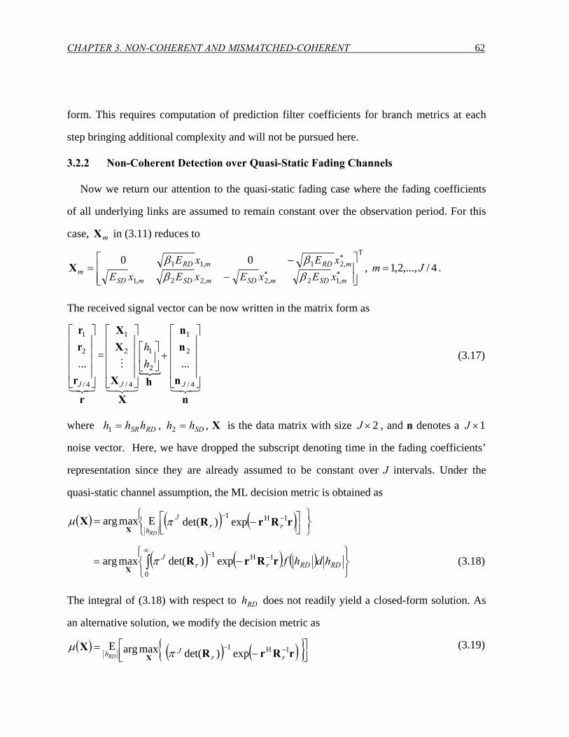
CHAPTER 3. NON-COHERENT AND MISMATCHED-COHERENT 62
form. This requires computation of prediction filter coefficients for branch metrics at each
step bringing additional complexity and will not be pursued here.
3.2.2 Non-Coherent Detection over Quasi-Static Fading Channels
Now we return our attention to the quasi-static fading case where the fading coefficients
of all underlying links are assumed to remain constant over the observation period. For this
case, mX in (3.11) reduces to Τ
∗∗
∗
⎥⎥⎦
⎤
⎢⎢⎣
⎡
−−
=mSDmSDmSDmSD
mRDmRDm xExExExE
xExE
,12,2,22,1
,21,11 00ββββ
X , 4/,...,2,1 Jm = .
The received signal vector can be now written in the matrix form as
321r
r
rr
⎥⎥⎥⎥
⎦
⎤
⎢⎢⎢⎢
⎣
⎡
4/
2
1
...
J
=
321321
M
n
n
nn
hX
X
XX
⎥⎥⎥⎥
⎦
⎤
⎢⎢⎢⎢
⎣
⎡
+⎥⎦
⎤⎢⎣
⎡
⎥⎥⎥⎥
⎦
⎤
⎢⎢⎢⎢
⎣
⎡
4/
2
1
2
1
4/
2
1
...
JJ
hh
(3.17)
where RDSRhhh =1 , SDhh =2 , X is the data matrix with size 2×J , and n denotes a 1×J
noise vector. Here, we have dropped the subscript denoting time in the fading coefficients’
representation since they are already assumed to be constant over J intervals. Under the
quasi-static channel assumption, the ML decision metric is obtained as
( ) ( ) ( )⎭⎬⎫
⎩⎨⎧
⎥⎦⎤
⎢⎣⎡ −= −Η− exp)det(Emaxarg 11
rRrRXX rr
J
hRD
πµ
( ) ( ) ( )⎭⎬⎫
⎩⎨⎧
−= ∫∞
−Η−
0
11exp)det(maxarg RDRDrr
J hdhfrRrRX
π (3.18)
The integral of (3.18) with respect to RDh does not readily yield a closed-form solution. As
an alternative solution, we modify the decision metric as
( ) ( ) ( ) ⎥⎦⎤⎢⎣⎡
−= −Η− exp)det( maxargE 11rRrRX
X rrJhRD πµ (3.19)
CHAPTER 3. NON-COHERENT AND MISMATCHED-COHERENT 63
Replacing (3.14) in (3.19), we have
( ) ( ) ( )( ) ( ) ⎥⎦⎤⎢⎣⎡ ++++= −ΗΗΗ detlnln minarg 1
00 rIXXRrIXXRXhhX JJh NNJE
RDπµ (3.20)
Using the matrix identity ( ) ( ) 1111111 −−−−−−− +−=+ DABDACBAABCDA [88], the argu-
ment of the determinant term in (3.20) can be rearranged as
( ) Η−
Η−−Η⎟⎟⎠
⎞⎜⎜⎝
⎛+−=+ XXXRXIIXXRh
1
0
1200
10
11NNN
N hJ
J . (3.21)
Further replacing ( )1,diag 2RDh=hR in (3.21) and exploiting the embedded orthogonality of
data sequence in the resulting expression, i.e.,
( )
( )( ) ⎥⎦
⎤⎢⎣
⎡+
=SD
RDH
EJEJ
12/002/
2
1
ββ
XX ,
we rewrite (3.21) as
( ) Η−Η −=+ XXΑIIXXRh 1200
10 NN
N JJ (3.22)
where A is defined by
( ) ⎥⎥⎥⎥⎥⎥⎥
⎦
⎤
⎢⎢⎢⎢⎢⎢⎢
⎣
⎡
++
+=
02
2
01
2
12
1
10
0
21
NEJ
hN
EJh
SD
RDRD
RD
β
βΑ .
Using the matrix identity ( ) ( )BAIABI +=+ detdet [88] and again exploiting the orthogo-
nality structure of the underlying STBC, the determinant term in (3.20) can be shown to be
independent of the data sequence. Replacing (3.22) in (3.20) and dropping unnecessary terms
which do not affect maximization, we obtain
CHAPTER 3. NON-COHERENT AND MISMATCHED-COHERENT 64
( )⎥⎥⎦
⎤
⎢⎢⎣
⎡
⎭⎬⎫
⎩⎨⎧−= rXAXrX
X
HH20
1minargENRDh
µ . (3.23)
The expectation of (3.23) with respect to RDh does not yield a closed-form solution for the
general case. In the following, we demonstrate that a closed-form decision metric can be ob-
tained imposing some assumptions on the underlying links.
Case 1 (Power control between DS → and DR → links and high SNR in RS →
link): Assume perfect power control where DS → and DR → links are balanced, i.e.,
00/ NENE SDRD = , and sufficiently large SNR for the RS → link, i.e.,
00/ NENE SDSR >> . Under these assumptions, A reduces to the form of
⎥⎥⎥⎥⎥⎥⎥
⎦
⎤
⎢⎢⎢⎢⎢⎢⎢
⎣
⎡
+
+=
0
2
0
2
1
10
0
21
NEJ
hN
JEh
SD
RDSD
RD
Α .
Replacing A in (3.23) and carrying out the expectation with respect RDh , we obtain the deci-
sion metric as
( ) 2maxarg rΦXX
X
H=µ (3.24)
where
( )( )⎥⎥⎥
⎦
⎤
⎢⎢⎢
⎣
⎡
+
Γ−=
0/110
0,01
NJE
e
SD
ψβψ ψ
Φ . (3.25)
with ( )0/2 NNESD=ψ and ( ).,.Γ denotes the incomplete gamma function [71]. Under the
assumption of 1// 0 >>= NENE SDRD , Φ further reduces to
CHAPTER 3. NON-COHERENT AND MISMATCHED-COHERENT 65
/10
0/
2
0
0
⎥⎥⎥⎥
⎦
⎤
⎢⎢⎢⎢
⎣
⎡
=
NJE
NJE
SD
SDΦ . (3.26)
Case 2 (Non-fading DR → link): Besides the assumptions imposed in Case 1, we also
now assume a non-fading DR → link. It can be easily shown that the decision metric is still
given by (3.24) where Φ is
( )
⎥⎥⎥⎥
⎦
⎤
⎢⎢⎢⎢
⎣
⎡
+
+=
0
0
/110
0/2/1
1
NJE
NEJ
SD
SDΦ . (3.27)
One can interestingly note that the derived decoding rule given by (3.24) has a similar
form to
( ) 2maxarg rXX
X
H=µ (3.28)
which is the quadratic non-coherent receiver derived earlier for conventional (i.e., non-
distributed) STBC in [89], [90]. Replacing Φ in (3.24) by an identity matrix, one can simply
obtain (3.28). In other words, (3.24) is a generalized version of the conventional decoder. In
the considered cooperative scenario, the effects of AaF relaying and path loss/shadowing as-
sociated with underlying relay links manifest themselves in (3.24) through the scaling matrix
Φ . Through the PEP derivations in the Appendix B.1, we demonstrate that the non-coherent
decoding rule is able to collect a diversity order of two which is the full diversity for the con-
sidered single-relay scenario. It should be noted that this diversity order is attainable for as-
ymptotically high SNR. In practical range of SNR values, the performance of distributed
STBC experiences some degradation in comparison to that of non-distributed STBC.
In the practical implementation of (3.24), one should notice that the quadratic nature of
(3.24) results in a phase ambiguity [89]. This ambiguity can be resolved easily by fixing the
CHAPTER 3. NON-COHERENT AND MISMATCHED-COHERENT 66
first symbol transmitted from each of the links to a specific value, i.e., insertion of a known
symbol at the beginning of the frame. Direct implementation of (3.24) is still impractical due
to substantial computational complexity. However, this time, unlike (3.15) and (3.16), it is
possible to develop a recursive expression from (3.24) which can be easily implemented by a
Viterbi-type algorithm. Expanding (3.24), we can readily obtain the desired recursive form as
( ) ( )⎪⎭
⎪⎬⎫
⎪⎩
⎪⎨⎧
⎥⎦
⎤⎢⎣
⎡+= ∑
−
−=
Η−1
),1max(
1 Rem
Imjiim
Hm
mm rΦXΦXrXX µµ , 4/,...1 Jm = (3.29)
where mX is defined earlier in (3.17). The inner term in (3.29) can be interpreted as a chan-
nel estimate based on a truncation interval of previous I sub-blocks. Although the derived
decoding rule is based on a quasi-static fading assumption, this inherent channel tracking
ability makes it a suitable candidate for deployment over time-varying channels.
3.3 Mismatched-Coherent Detection for Distributed STBCs
In this section, we consider a mismatched-coherent receiver, i.e., coherent detection with
imperfect channel estimation, as a possible alternative to the non-coherent receiver proposed
in the previous section. For channel estimation purposes, we employ pilot symbols (i.e., a set
of symbols whose location and values are known to the receiver) multiplexed with the infor-
mation-bearing data. To the best of our knowledge, pilot-symbol-assisted channel estimation
has not been yet fully studied in the context of cooperative communication.
3.3.1 Mismatched-Coherent Detection over Quasi-Static Fading Channels
Let TX denote the pilot symbol matrix transmitted by the source terminal followed by a
data matrix DX . Under the assumption that fading coefficients are constant over the entire
transmission frame, the received signals during the training and data transmission phases are
given, respectively, as
CHAPTER 3. NON-COHERENT AND MISMATCHED-COHERENT 67
TTT nhXr += (3.30)
DDD nhXr += (3.31)
where ( )T21,hh=h with RDSRhhh =1 and SDhh =2 . In (3.30)-(3.31), the entries of Tn and
Dn are zero-mean complex Gaussian random variables with variance 20N per dimension.
The channel coefficients are first estimated using Tr and TX to obtain the channel estimate
h , which can be then used to minimize the following coherent ML metric as if the channel
was perfectly known.
( ) 2ˆminarg hXrXX DDD
D
−=µ . (3.32)
The performance of the mismatched receiver relies on the choice of the channel estimator.
Here, we consider ML and linear-minimum-mean-square-error (LMMSE) estimators.
ML Estimator: Conditioned on h and TX , the ML estimate of the channel matrix is amount
to minimizing 2hXr TT − with respect to h. Therefore, under the same SNR assumptions,
(i.e., 00/ NENE SDRD = , 00/ NENE SDSR >> ) imposed in the previous section, the ML esti-
mate of h is given as [91]
( ) TTTTML rXXXh Η−Η=1ˆ . (3.33)
Replacing (3.30) in (3.33), we obtain
MLML εhh +=ˆ (3.34)
where we define the channel estimation error vector ( ) TTTTML nXXXε Η−Η=1
with covariance
matrix
[ ]⎥⎥⎥⎥
⎦
⎤
⎢⎢⎢⎢
⎣
⎡
=Η
0
0
/10
0/5.0
1
E
NPE
NPE
SD
SDMLMLεε . (3.35)
where P denotes the number pilot symbols.
CHAPTER 3. NON-COHERENT AND MISMATCHED-COHERENT 68
LMMSE estimator: The LMMSE estimate of the channel matrix is obtained by the linear
transformation TBr , where B minimizes ][ 2hBr −TE . Hence, the channel estimate LMMSEh
is given as [92]
( ) TTTTLMMSE N rXRXXh hΗ−−Η +=
110
ˆ (3.36)
where hR is the autocorrelation matrix of h . Replacing (3.30) in (3.36), we obtain
( ) LMMSETTTTLMMSE N εhXXRXXh h ++= Η−−Η 110
ˆ (3.37)
where channel estimation error vector is defined as ( ) TTTTLMMSE N nXRXXε hΗ−−Η +=
110 . Under
the assumption of ∞→0/ NESD , the covariance matrix of LMMSEε converges to (3.35) of ML
estimator. In Appendix B.2, we demonstrate through PEP derivation that the mismatched-
coherent receiver is able to achieve full diversity order over quasi-static channels.
3.3.2 Mismatched-Coherent Detection over Time-Varying Fading Channels
In this subsection, we assume all underlying links experience time-selectivity. In the con-
sidered single-relay scenario, Alamouti-coded pilot symbols are sent over four time slots:
Specifically, in time slot k , the source terminal simultaneously transmits the pilot symbol 1p
to the destination terminal and the relay terminal. In time slot k+1, the relay terminal trans-
mits the received version of pilot symbol (after energy normalization) to the destination ter-
minal. In the same time slot, the source terminal transmits the other pilot symbol 2p to the
destination terminal. The same procedure is repeated for the transmission of ∗− 2p and .1∗p
The destination terminal makes an observation of L frames, each of which consists of J sym-
bols and extracts 4L observations of the nearest pilot symbols for channel estimation purpose
(see Figure 3.2).
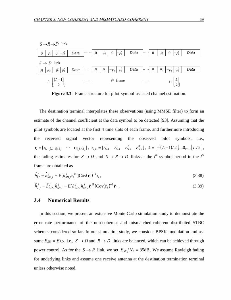
CHAPTER 3. NON-COHERENT AND MISMATCHED-COHERENT 69
0 1p 0 ∗− 2p
1p 2p ∗− 2p∗1p
Data
Data
0 1p 0 ∗− 2p
1p 2p ∗− 2p ∗1p
Data
Data
0 1p 0 ∗− 2p
1p 2p ∗− 2p ∗1p
Data
Data
thl frame( )⎥⎦⎥
⎢⎣⎢ −
−2
1Ll ⎥⎦⎥
⎢⎣⎢+
2Ll
DRS →→
DS →
link
link
Figure 3.2: Frame structure for pilot-symbol-assisted channel estimation.
The destination terminal interpolates these observations (using MMSE filter) to form an
estimate of the channel coefficient at the data symbol to be detected [93]. Assuming that the
pilot symbols are located at the first 4 time slots of each frame, and furthermore introducing
the received signal vector representing the observed pilot symbols, i.e.,
( )⎣ ⎦ ⎣ ⎦][ 2/,2/1, LlLll rrr L−−= , ][ 3210, klklklklkl rrrr ++++=r , ( )⎣ ⎦ ⎣ ⎦2/,...,0,...2/1 LLk −−= ,
the fading estimates for DS → and DRS →→ links at the jth symbol period in the lth
frame are obtained as
( ) lllj
lSDj
lSDjl hhh rrr 1
,,,1 ]CovE[ˆˆ −Η== , (3.38)
( ) lllj
lSRj
lRDj
lSRj
lRDj
j hhhhh rrr 1,,,,.2 Cov][Eˆˆˆ −Η== . (3.39)
3.4 Numerical Results
In this section, we present an extensive Monte-Carlo simulation study to demonstrate the
error rate performance of the non-coherent and mismatched-coherent distributed STBC
schemes considered so far. In our simulation study, we consider BPSK modulation and as-
sume RDSD EE = , i.e., DS → and DR → links are balanced, which can be achieved through
power control. As for the RS → link, we set dB350 =NESR . We assume Rayleigh fading
for underlying links and assume one receive antenna at the destination termination terminal
unless otherwise noted.
CHAPTER 3. NON-COHERENT AND MISMATCHED-COHERENT 70
In Figure 3.3, we present the bit error rate (BER) performance of the ML-optimum decod-
ing rule given by (3.18) implemented through exhaustive search over all possible sequences,
and the derived decoding rule given by (3.24) in conjunction with scaling matrix Φ given by
(3.25), (3.26), and (3.27). We assume quasi-static fading for all underlying links. It is ob-
served that optimum decoding rule and proposed decoder yield nearly identical performance.
This is very promising since the implementation complexity of (3.24) is much lower than the
optimum decoder which requires multi-dimensional integral and does not yield a closed-form
solution.
It is also interesting to observe that different forms of scaling matrix Φ , i.e., (3.25) and
(3.27) do not result in a significant change in the performance although they have been ob-
tained under the assumption of fading and non-fading DR → links, respectively. One can
also note that (3.26) is the simplified version of (3.25) under high SNR assumption (see the
discussion in Section 3.2.2). Considering the nearly identical performance observed for three
different scaling matrices, (3.26) and (3.27) are favorable choices since they avoid the use of
incomplete gamma function unlike (3.25). As a benchmark, we also investigate the perform-
ance of the non-coherent decoder rule given by (3.28) for conventional (non-distributed)
STBC within the considered cooperative scenario. It is observed that there is a performance
loss of dB1≈ at BER 310−= . This performance degradation further decreases with the in-
creasing number of receive antennas employed at the destination terminal. It should be em-
phasized (3.28) does not require any kind of information on the underlying links unlike
(3.25)-(3.26)-(3.27) which need average SNR estimation for the underlying links. Therefore,
(3.28) can be possibly used as an alternative sub-optimal detector for distributed STBC.
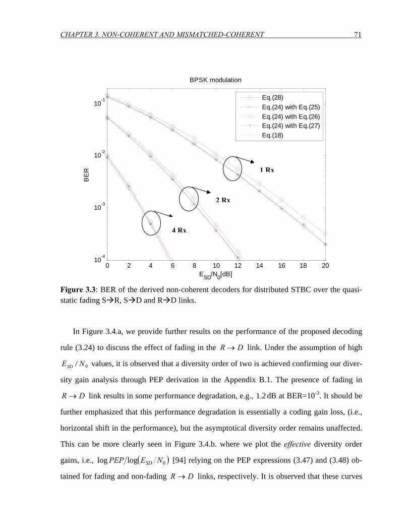
CHAPTER 3. NON-COHERENT AND MISMATCHED-COHERENT 71
0 2 4 6 8 10 12 14 16 18 2010-4
10-3
10-2
10-1
ESD/N0[dB]
BE
RBPSK modulation
Eq.(28)Eq.(24) with Eq.(25)Eq.(24) with Eq.(26)Eq.(24) with Eq.(27)Eq.(18)
Figure 3.3: BER of the derived non-coherent decoders for distributed STBC over the quasi-static fading S R, S D and R D links.
In Figure 3.4.a, we provide further results on the performance of the proposed decoding
rule (3.24) to discuss the effect of fading in the DR → link. Under the assumption of high
0/ NESD values, it is observed that a diversity order of two is achieved confirming our diver-
sity gain analysis through PEP derivation in the Appendix B.1. The presence of fading in
DR → link results in some performance degradation, e.g., 2.1 dB at BER=10-3. It should be
further emphasized that this performance degradation is essentially a coding gain loss, (i.e.,
horizontal shift in the performance), but the asymptotical diversity order remains unaffected.
This can be more clearly seen in Figure 3.4.b. where we plot the effective diversity order
gains, i.e., ( )0loglog NEPEP SD [94] relying on the PEP expressions (3.47) and (3.48) ob-
tained for fading and non-fading DR → links, respectively. It is observed that these curves
1 Rx
2 Rx
4 Rx
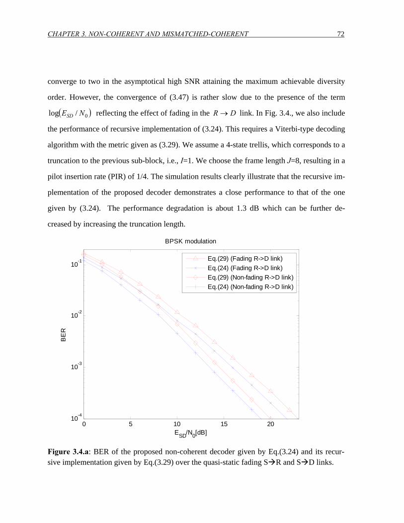
CHAPTER 3. NON-COHERENT AND MISMATCHED-COHERENT 72
converge to two in the asymptotical high SNR attaining the maximum achievable diversity
order. However, the convergence of (3.47) is rather slow due to the presence of the term
( )0/log NESD reflecting the effect of fading in the DR → link. In Fig. 3.4., we also include
the performance of recursive implementation of (3.24). This requires a Viterbi-type decoding
algorithm with the metric given as (3.29). We assume a 4-state trellis, which corresponds to a
truncation to the previous sub-block, i.e., I=1. We choose the frame length J=8, resulting in a
pilot insertion rate (PIR) of 1/4. The simulation results clearly illustrate that the recursive im-
plementation of the proposed decoder demonstrates a close performance to that of the one
given by (3.24). The performance degradation is about 1.3 dB which can be further de-
creased by increasing the truncation length.
0 5 10 15 2010-4
10-3
10-2
10-1
ESD/N0[dB]
BE
R
BPSK modulation
Eq.(29) (Fading R->D link)Eq.(24) (Fading R->D link)Eq.(29) (Non-fading R->D link)Eq.(24) (Non-fading R->D link)
Figure 3.4.a: BER of the proposed non-coherent decoder given by Eq.(3.24) and its recur-sive implementation given by Eq.(3.29) over the quasi-static fading S R and S D links.
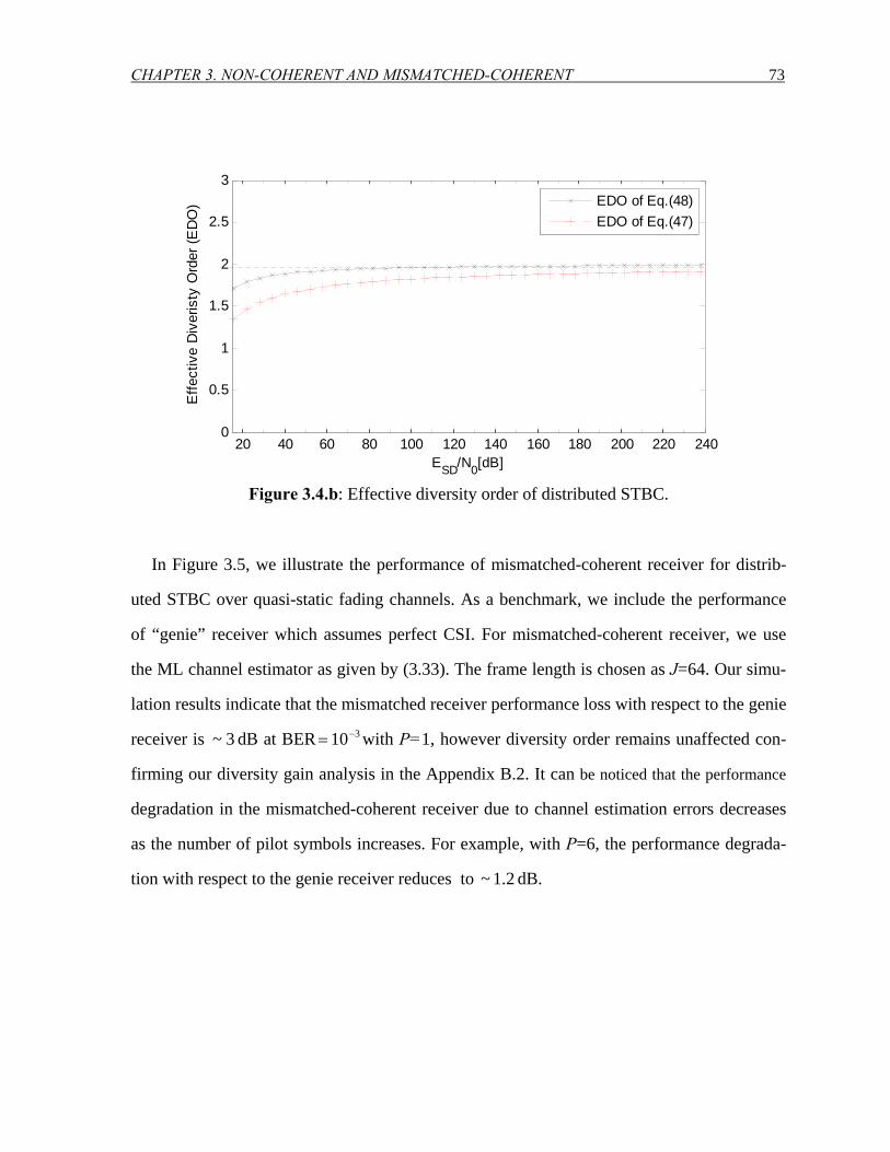
CHAPTER 3. NON-COHERENT AND MISMATCHED-COHERENT 73
20 40 60 80 100 120 140 160 180 200 220 2400
0.5
1
1.5
2
2.5
3
ESD/N0[dB]
Effe
ctiv
e D
iver
isty
Ord
er (E
DO
)
EDO of Eq.(48)EDO of Eq.(47)
Figure 3.4.b: Effective diversity order of distributed STBC.
In Figure 3.5, we illustrate the performance of mismatched-coherent receiver for distrib-
uted STBC over quasi-static fading channels. As a benchmark, we include the performance
of “genie” receiver which assumes perfect CSI. For mismatched-coherent receiver, we use
the ML channel estimator as given by (3.33). The frame length is chosen as J=64. Our simu-
lation results indicate that the mismatched receiver performance loss with respect to the genie
receiver is 3~ dB at BER 310−= with P=1, however diversity order remains unaffected con-
firming our diversity gain analysis in the Appendix B.2. It can be noticed that the performance
degradation in the mismatched-coherent receiver due to channel estimation errors decreases
as the number of pilot symbols increases. For example, with P=6, the performance degrada-
tion with respect to the genie receiver reduces to 2.1~ dB.
CHAPTER 3. NON-COHERENT AND MISMATCHED-COHERENT 74
In Figure 3.5, we also include the performance of the non-coherent decoder for further
comparison with mismatched-coherent receiver. Assuming P=11, the proposed non-coherent
receiver given by (3.24) outperforms the mismatched-coherent receiver by 8.1~ dB at
BER 310−= . The recursive implementation of the non-coherent receiver given by (3.29) still
outperforms the mismatched-coherent receiver by 5.0~ dB at BER 310−= . With the increas-
ing number of pilot symbols (therefore at the cost of decreasing throughput), mismatched-
coherent receiver is able to provide a better performance in comparison to its competitor. For
example, with P=6, mismatched-coherent receiver outperforms the recursive implementation
of the non-coherent receiver by 2~ dB at BER 310−= and is 2.1~ dB away from the genie
receiver performance.
In Figure 3.6, we consider a time-varying channel scenario and present a performance
comparison of non-coherent and mismatched-coherent receivers. We assume that RS → and
DS → fading links experience Bessel-type autocorrelation function, i.e., Jakes Channel
model, with normalized Doppler values of =SRfT 01.0=SDfT . A non-fading channel is as-
sumed for the DR → link. We observe that the recursive implementation of the proposed
non-coherent receiver, i.e. (3.29), still demonstrates close results in comparison to the opti-
mum decoder given by (3.16) for time-varying channels although it is originally derived un-
der the quasi-static channel assumption. For the mismatched-coherent receiver, pilot-symbol
assisted channel estimator with Wiener filter is used as described in Section 3.3.2. The esti-
mated fading coefficients are then used to minimize the metric given by (3.32). For both non-
coherent and mismatched-coherent receivers, we use pilot insertion rate (PIR) =1/4, there-
1 It should be noted that only one pilot symbol is required for the non-coherent decoder to resolve the phase ambiguity.
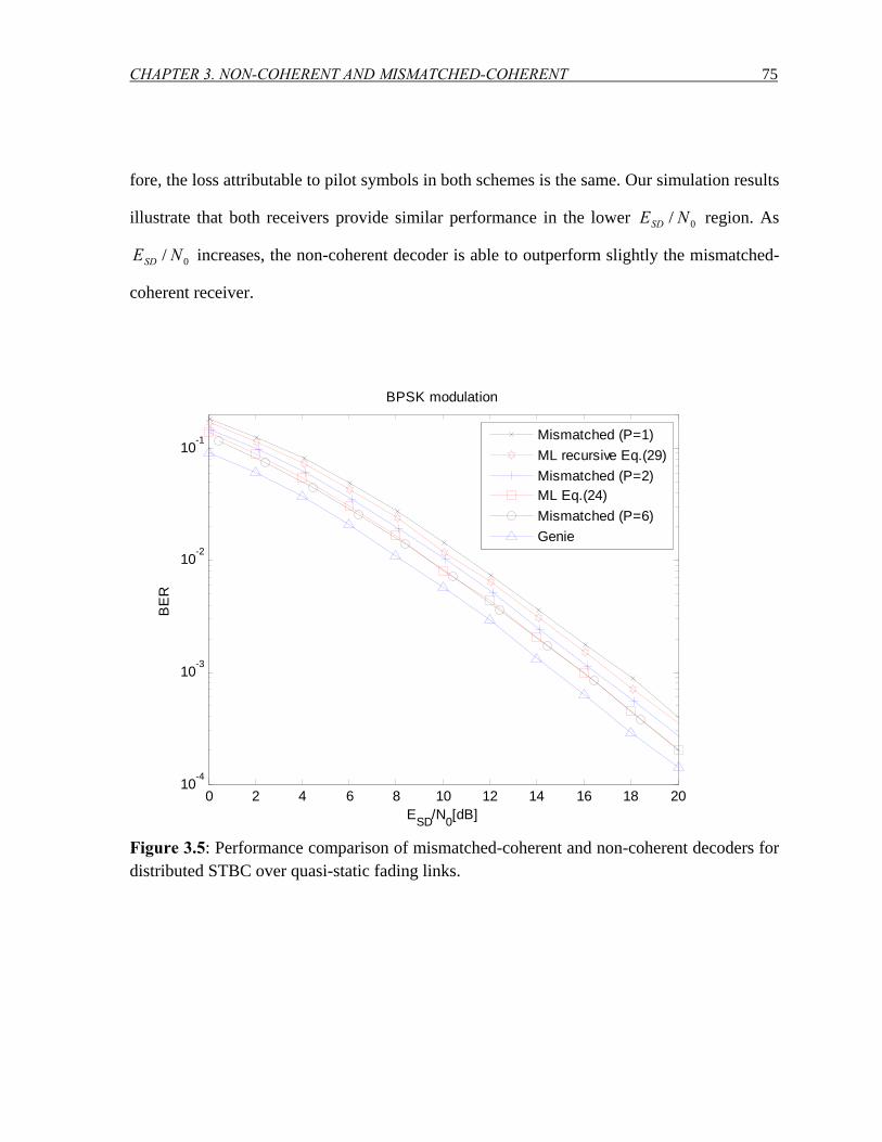
CHAPTER 3. NON-COHERENT AND MISMATCHED-COHERENT 75
fore, the loss attributable to pilot symbols in both schemes is the same. Our simulation results
illustrate that both receivers provide similar performance in the lower 0/ NESD region. As
0/ NESD increases, the non-coherent decoder is able to outperform slightly the mismatched-
coherent receiver.
0 2 4 6 8 10 12 14 16 18 2010-4
10-3
10-2
10-1
ESD/N0[dB]
BE
R
BPSK modulation
Mismatched (P=1)ML recursive Eq.(29)Mismatched (P=2)ML Eq.(24)Mismatched (P=6)Genie
Figure 3.5: Performance comparison of mismatched-coherent and non-coherent decoders for distributed STBC over quasi-static fading links.
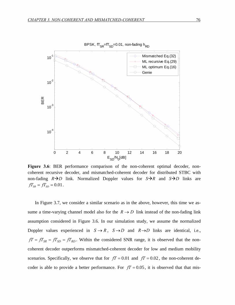
CHAPTER 3. NON-COHERENT AND MISMATCHED-COHERENT 76
0 2 4 6 8 10 12 14 16 18 20
10-4
10-3
10-2
10-1
ESD/N0[dB]
BE
RBPSK, fTSR=fTSD=0.01, non-fading hRD
Mismatched Eq.(32)ML recursive Eq.(29)ML optimum Eq.(16)Genie
Figure 3.6: BER performance comparison of the non-coherent optimal decoder, non-coherent recursive decoder, and mismatched-coherent decoder for distributed STBC with non-fading R D link. Normalized Doppler values for S R and S D links are
01.0== SDSR fTfT .
In Figure 3.7, we consider a similar scenario as in the above, however, this time we as-
sume a time-varying channel model also for the DR → link instead of the non-fading link
assumption considered in Figure 3.6. In our simulation study, we assume the normalized
Doppler values experienced in RS → , DS → and DR→ links are identical, i.e.,
RDSDSR fTfTfTfT === . Within the considered SNR range, it is observed that the non-
coherent decoder outperforms mismatched-coherent decoder for low and medium mobility
scenarios. Specifically, we observe that for 01.0=fT and 02.0=fT , the non-coherent de-
coder is able to provide a better performance. For 05.0=fT , it is observed that that mis-
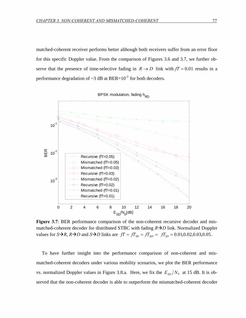
CHAPTER 3. NON-COHERENT AND MISMATCHED-COHERENT 77
matched-coherent receiver performs better although both receivers suffer from an error floor
for this specific Doppler value. From the comparison of Figures 3.6 and 3.7, we further ob-
serve that the presence of time-selective fading in DR → link with 01.0=fT results in a
performance degradation of ~3 dB at BER=10-3 for both decoders.
0 2 4 6 8 10 12 14 16 18 20
10-3
10-2
10-1
ESD/N0[dB]
BE
R
BPSK modulation, fading hRD
Recursive (fT=0.05)Mismatched (fT=0.05)Mismatched (fT=0.03)Recursive (fT=0.03)Mismatched (fT=0.02)Recursive (fT=0.02)Mismatched (fT=0.01)Recursive (fT=0.01)
Figure 3.7: BER performance comparison of the non-coherent recursive decoder and mis-matched-coherent decoder for distributed STBC with fading R D link. Normalized Doppler values for S R, R D and S D links are === RDSR fTfTfT 05.0,03.0,02.0,01.0=SDfT .
To have further insight into the performance comparison of non-coherent and mis-
matched-coherent decoders under various mobility scenarios, we plot the BER performance
vs. normalized Doppler values in Figure 3.8.a. Here, we fix the 0NESD at 15 dB. It is ob-
served that the non-coherent decoder is able to outperform the mismatched-coherent decoder
CHAPTER 3. NON-COHERENT AND MISMATCHED-COHERENT 78
for low and intermediate Doppler values. For higher Doppler values, it can be seen that the
mismatched-coherent decoder outperforms its competitor. In Figure 3.8.b., we further let the
Doppler values in the underlying links be different from each other. Specifically, we assume
the following three scenarios:
S.1) 01.0== SDRD fTfT and ]06.0,01.0[== fTfTSR .
S.2) 01.0== SDSR fTfT and fTfTRD = = ]06.0,01.0[ .
S.3) 01.0== RDSR fTfT and fTfTSD = = ]06.0,01.0[ .
Our simulation results reveal that the first two scenarios yield identical performance. This is
due the symmetrical structure of RS → and DR → links in the cascaded relay channel.
Thus, for the sake of presentation simplicity, we only include the performance of the first
scenario in the figure. For scenarios in S.1) and S.3), we observe that the non-coherent de-
coder is able to outperform mismatched-coherent decoder for normalized Doppler values less
than 045.0 and 015.0 , respectively.
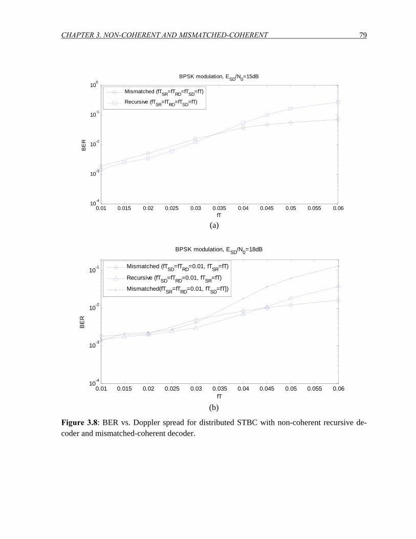
CHAPTER 3. NON-COHERENT AND MISMATCHED-COHERENT 79
0.01 0.015 0.02 0.025 0.03 0.035 0.04 0.045 0.05 0.055 0.0610-4
10-3
10-2
10-1
100
fT
BE
RBPSK modulation, ESD/N0=15dB
Mismatched (fTSR=fTRD=fTSD=fT)
Recursive (fTSR=fTRD=fTSD=fT)
(a)
0.01 0.015 0.02 0.025 0.03 0.035 0.04 0.045 0.05 0.055 0.0610-4
10-3
10-2
10-1
fT
BE
R
BPSK modulation, ESD/N0=18dB
Mismatched (fTSD=fTRD=0.01, fTSR=fT)
Recursive (fTSD=fTRD=0.01, fTSR=fT)
Mismatched(fTSR=fTRD=0.01, fTSD=fT])
(b)
Figure 3.8: BER vs. Doppler spread for distributed STBC with non-coherent recursive de-coder and mismatched-coherent decoder.
CHAPTER 3. NON-COHERENT AND MISMATCHED-COHERENT 80
Appendix B
In this section, we present a diversity gain analysis for the non-coherent and coherent
mismatched detectors through the derivation of PEP.
B.1 PEP Derivation for Non-coherent Detector
Let the transmitted codeword be [ ]Τ= 4/21 ,...,, Jc XXXX . Conditioned on RDh , the as-
ymptotic PEP for non-coherent receivers is readily found as [95-Eq.28] k
ee
cc
kmmRDec k
khP ⎟
⎟⎠
⎞⎜⎜⎝
⎛⎟⎟⎠
⎞⎜⎜⎝
⎛⎟⎟⎠
⎞⎜⎜⎝
⎛ −⎟⎟⎠
⎞⎜⎜⎝
⎛=→ ∑∏
=
−
= RR
XX ln!
12
4)|(
2
0
12
1λ (3.40)
where cccc XXR Η= and eeee XXR Η= denote the autocorrelation matrices of eX and cX , re-
spectively. In (3.40), ,mλ 2,1=m are the positive eigenvalues of the matrix
( ) )(/ cecce κκXRΨ r −= where Ncccr IΣXXXR += Η/ , ( ) Η−−+−= ccccc XΣRXκ11 , and
( ) Η−−+−= eeeee XΣRXκ11 . Here, Σ is defined as
( )( )⎥
⎥⎦
⎤
⎢⎢⎣
⎡=
02
201
00
NEhNE
SD
RDRD
ββΣ . (3.41)
Using the definitions of eκ and cκ , we can write ceΨ in the following form
( ) ( ) ( ) ⎟⎠⎞⎜
⎝⎛ +−++= Η−−Η−−Η
eeeeccccNccce XΣRXXΣRXIΣXXΨ1111 . (3.42)
where we define the cross-correlation matrices of eX and cX as ecce XXR Η= and
ceec XXR Η= . After some algebra and using the fact that the non-zero eigenvalues of AB and
BA are equal [88], we can rewrite (3.42) as
( ) ( ) ( ) ( ) eeeecccceceececcccccce RRΣRRΣRRΣΣRRRΣΣRΨ11111111 −−−−−−−− +−+++−+= (3.43)
Under the high SNR assumption, i.e., 1// 00 >>>> NENE SDSR and
1// 00 >>>> NENE RDSR , the 1−Σ term can be ignored and (3.43) reduces to
( )( )eceececcce RRRRΣΨ 1−−= . (3.44)
CHAPTER 3. NON-COHERENT AND MISMATCHED-COHERENT 81
The eigenvalues of ceΨ are then obtained as ( ) 12
01 χRDRD hNEλ = and ( ) 202 χNEλ SD=
where iχ , 2,1=i denote the eigenvalues of ( )( )eceececc RRRR 1−− . Replacing the eigenvalues
of (3.44) in (3.40) and noting eecc RR = (due to the orthogonal structure), (3.40) simplifies
to2
1
20
12
10
0
6)(−−
⎟⎟⎠
⎞⎜⎜⎝
⎛⎟⎟
⎠
⎞
⎜⎜
⎝
⎛⎟⎟⎠
⎞⎜⎜⎝
⎛+≈→
→
χδχδ
NE
hN
EEP SD
RDRD
heeccRD
XX . (3.45)
Under the assumption of perfect power control, i.e., RDSD EE = , the unconditional PEP for
the non-coherent receiver is found as
⎟⎟⎠
⎞⎜⎜⎝
⎛Γ⎟⎟
⎠
⎞⎜⎜⎝
⎛⎟⎟⎠
⎞⎜⎜⎝
⎛≈→
−
⎟⎟⎠
⎞⎜⎜⎝
⎛−
=
−
∏ 10
12
1
2
0,06)(
1
10 χδχχδ
NE
eNE
P SDNE
ii
SDeecc
SD
XX . (3.46)
where ( ).,.Γ denotes the incomplete gamma function [71]. Using the limiting expression
( )zz log),0( −≈Γ for 0→z [71] and noting that ( ) 11
0/1 ≈−NSDEe χδ , we can write (3.46) as
( ) ⎟⎟⎠
⎞⎜⎜⎝
⎛⎟⎟⎠
⎞⎜⎜⎝
⎛⎟⎟⎠
⎞⎜⎜⎝
⎛≈→ ∏
=
− 2
10
2
0log6
ii
SDSDeecc N
ENE
P χXX . (3.47)
For sufficiently high 0/ NESD , the term ( )0/log NESD can be ignored with respect to the
dominating term of ( ) 20/ −NESD . Thus, asymptotically, the second order diversity is
achieved, realizing the maximum achievable diversity for the considered scenario with single
relay. It should be pointed out that for a non-fading DR → link assumption, i.e., 1=RDh ,
(3.45) simply reduces to
12
1
2
06)(
−
=
−
⎟⎟⎠
⎞⎜⎜⎝
⎛⎟⎟⎠
⎞⎜⎜⎝
⎛≈→ ∏
ii
SDeecc N
EP χXX . (3.48)
2 Due to the underlying assumptions in the derivation, PEP expression is an approximation, rather than the exact expression given by (3.40).
CHAPTER 3. NON-COHERENT AND MISMATCHED-COHERENT 82
which has a similar form to the PEP expression derived for conventional STBC with 2 trans-
mit and one receive antenna, c.f., [95-Eq.28]. Comparison of (3.47) and (3.48) further reveals
that, asymptotically, the factor ( )0/log NESD incurs a coding gain loss only.
B.2 PEP Derivation for Mismatched-Coherent Detector
In this section, we present a diversity gain analysis for the mismatched-coherent detector
with LMMSE channel estimator considered in Section 3.3.1. We assume perfect power con-
trol where DS → and DR → links are balanced, i.e., 1/ 00 >>= NENE SDRD , and sufficiently
large SNR for the RS → link, i.e., 00/ NENE SDSR >> . Noting that the channel estimate
LMMSEh and the channel estimation error LMMSEε are uncorrelated and omitting the subscript
LMMSE in (3.37), we can rewrite (3.31) in scalar form as
jDii
jiD hxrj
η+=∑=
ˆ2
1, 1,...,0 −= Jj (3.49)
where we define jDii ji nxjD +−= ∑ = εη 2
1 which is complex Gaussian with variance of
02
122 NE iSD ij+= ∑ = εη σσ . In (3.49), jix denotes the data symbol transmitted over the ith link at
time j. Notice that 01 =jx for 2,...,2,0 −= Jj . Noting that the decoder metric is given
by ,ˆ1
2∑ = −J
j ijiD hxrj
the Chernoff bound on the conditional PEP is then given as
( ) ( )⎟⎟⎠
⎞⎜⎜⎝
⎛
Ω−≤→
4
ˆ,expˆ|ˆ2
DDDD
dP XXhXX (3.50)
with
( ) ( )∑ ∑= =
−=J
j iijijiDD hxxd
1
22
1
2 ˆˆˆ,XX SDSD EhEh2
222
11ˆ~ˆ~ λλ += (3.51)
where iλ~ , 2,1=i denote the eigenvalues of ( ) ( )DDDD XXXX ˆˆ −−
Η and
22
1
20 jiiSDEN ηε σσ ≥+=Ω ∑=
. Defining the covariance matrix
( )22221
1 ,diag)ˆcov( εε σσ ++= RDhh for the estimated channel coefficients Τ= ]ˆˆ[ˆ21 hhh , we
can obtain the unconditional PEP as
CHAPTER 3. NON-COHERENT AND MISMATCHED-COHERENT 83
( )221
2
21~~1
4)ˆ,(
εσλλ +⎟⎠⎞
⎜⎝⎛
Ω≤
−SD
DDE
P XX ⎟⎟⎠
⎞⎜⎜⎝
⎛+
ΩΓ⎟⎟⎠
⎞⎜⎜⎝
⎛+
Ω 2
1
2
111 ~
4,0~4exp εε σ
λσ
λ SDSD EE. (3.52)
Using the limiting expression ( )zzz
log),0(lim0
−≈Γ→
[71], we can write (3.52) as
( )221
2
21~~1log
4)ˆ,(
εσλλ +⎟⎠⎞
⎜⎝⎛Ω
⎟⎠⎞
⎜⎝⎛
Ω≤
−SDSD
DDEE
P XX . (3.53)
For large Ω/SDE values, the term ( )Ω/log SDE can be ignored with respect to the dominating
term of ( ) 2/ −ΩSDE . Thus, asymptotically, the second order diversity is achieved, realizing
the maximum achievable diversity for the considered scenario with single relay. Further-
more, we observe that the presence of channel estimation errors does not affect the diversity
order. Similar observations have been earlier reported for conventional space time coding in
[96]-[98]. It should noted that as ∞→P , we have 02221== εε σσ , thus reducing (3.52) to
⎟⎟⎠
⎞⎜⎜⎝
⎛Γ⎟⎟⎠
⎞⎜⎜⎝
⎛⎟⎟⎠
⎞⎜⎜⎝
⎛≤
−
SDSD
SDDD E
NEN
NE
P1
0
1
02
021~4
,0~4
exp4~~
1)ˆ,(λλλλ
XX (3.54)
which was earlier reported in [33] for perfect CSI.
84
Chapter 4
Cooperative Communication with Multiple-Antenna Nodes
Introduction
So far, we have focused on cooperative communication scenarios where each node is
equipped with single transmit and receive antennas. In this chapter, we investigate the effect
of multiple antenna deployment assuming different relaying techniques. Specifically, we
consider Protocol II with blind AaF, CSI-assisted AaF, DaF relaying and quantify analyti-
cally the impact of multiple antenna deployment at the source, relay and/or destination termi-
nals on the diversity order for each of the relaying methods under consideration.
4.1 Transmission Model
We consider a wireless communication scenario where the source terminal S transmits in-
formation to the destination terminal D with the assistance of a single relay terminal R (c.f.
Fig. 4.1). The source and destination are equipped with SM and N antennas, respectively.
The relay terminal is equipped with RM receive and TM transmit antennas. We further as-
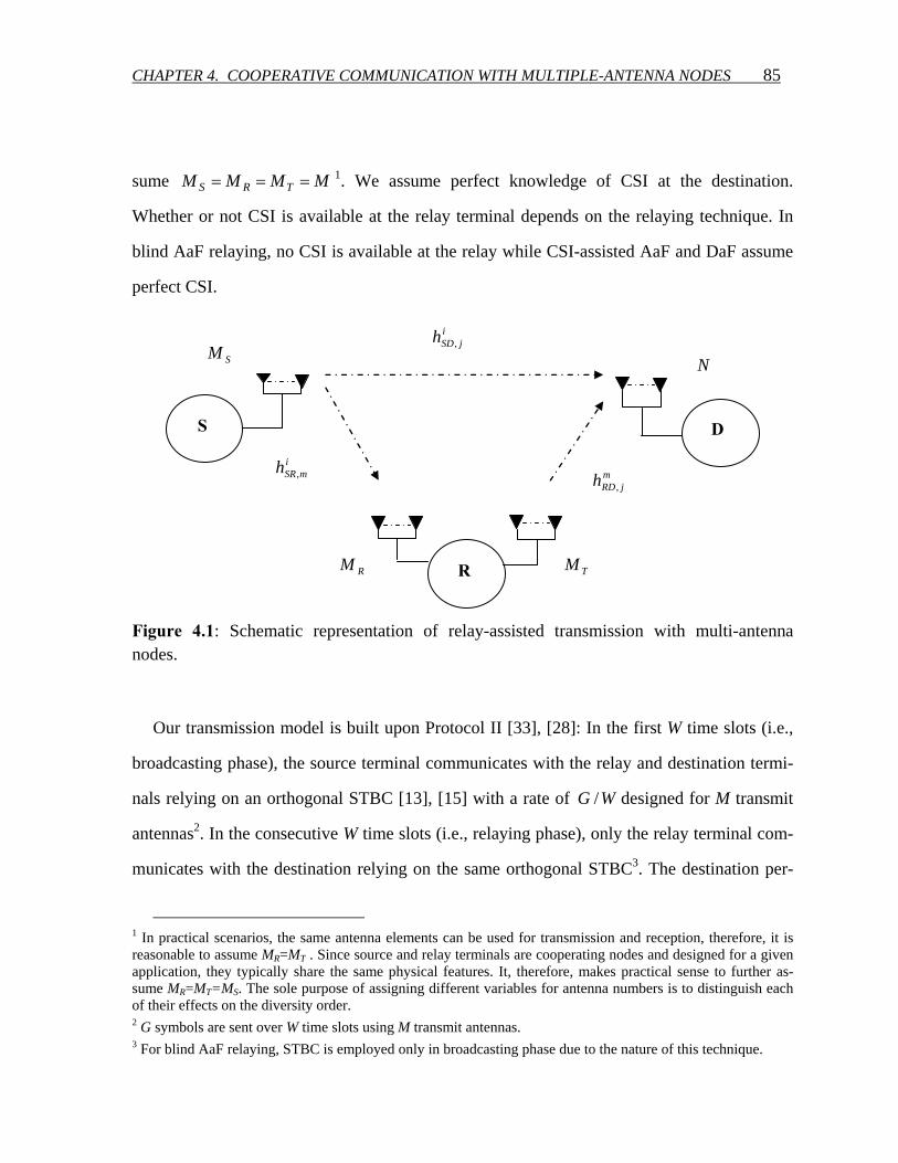
CHAPTER 4. COOPERATIVE COMMUNICATION WITH MULTIPLE-ANTENNA NODES 85
sume MMMM TRS === 1. We assume perfect knowledge of CSI at the destination.
Whether or not CSI is available at the relay terminal depends on the relaying technique. In
blind AaF relaying, no CSI is available at the relay while CSI-assisted AaF and DaF assume
perfect CSI.
i
jSDh , N
R
S D
imSRh , m
jRDh ,
SM
RM TM
Figure 4.1: Schematic representation of relay-assisted transmission with multi-antenna nodes.
Our transmission model is built upon Protocol II [33], [28]: In the first W time slots (i.e.,
broadcasting phase), the source terminal communicates with the relay and destination termi-
nals relying on an orthogonal STBC [13], [15] with a rate of WG / designed for M transmit
antennas2. In the consecutive W time slots (i.e., relaying phase), only the relay terminal com-
municates with the destination relying on the same orthogonal STBC3. The destination per-
1 In practical scenarios, the same antenna elements can be used for transmission and reception, therefore, it is reasonable to assume MR=MT . Since source and relay terminals are cooperating nodes and designed for a given application, they typically share the same physical features. It, therefore, makes practical sense to further as-sume MR=MT=MS. The sole purpose of assigning different variables for antenna numbers is to distinguish each of their effects on the diversity order.
2 G symbols are sent over W time slots using M transmit antennas.
3 For blind AaF relaying, STBC is employed only in broadcasting phase due to the nature of this technique.
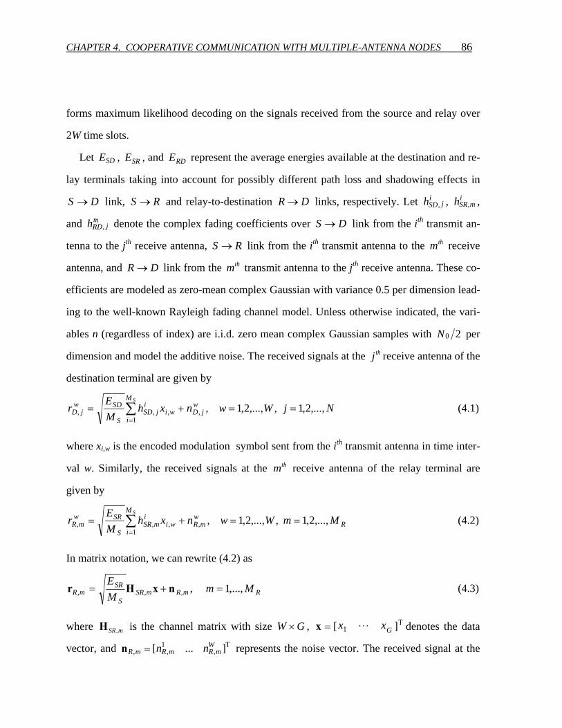
CHAPTER 4. COOPERATIVE COMMUNICATION WITH MULTIPLE-ANTENNA NODES 86
forms maximum likelihood decoding on the signals received from the source and relay over
2W time slots.
Let SDE , SRE , and RDE represent the average energies available at the destination and re-
lay terminals taking into account for possibly different path loss and shadowing effects in
DS → link, RS → and relay-to-destination DR → links, respectively. Let ijSDh , , i
mSRh , ,
and mjRDh , denote the complex fading coefficients over DS → link from the ith transmit an-
tenna to the jth receive antenna, RS → link from the ith transmit antenna to the thm receive
antenna, and DR → link from the thm transmit antenna to the jth receive antenna. These co-
efficients are modeled as zero-mean complex Gaussian with variance 0.5 per dimension lead-
ing to the well-known Rayleigh fading channel model. Unless otherwise indicated, the vari-
ables n (regardless of index) are i.i.d. zero mean complex Gaussian samples with 20N per
dimension and model the additive noise. The received signals at the thj receive antenna of the
destination terminal are given by
NjWwnxhME
rSM
i
wjDwi
ijSD
S
SDwjD ,...,2,1 ,,...,2,1 ,
1,,,, ==+= ∑
= (4.1)
where xi,w is the encoded modulation symbol sent from the ith transmit antenna in time inter-
val w. Similarly, the received signals at the thm receive antenna of the relay terminal are
given by
R
M
i
wmRwi
imSR
S
SRwmR MmWwnxh
ME
rS
,...,2,1 ,,...,2,1 ,1
,,,, ==+= ∑=
(4.2)
In matrix notation, we can rewrite (4.2) as
RmRmSRS
SRmR Mm
ME
,...,1 ,,,, =+= nxHr (4.3)
where mSR,H is the channel matrix with size GW × , Τ= ][ 1 Gxx Lx denotes the data
vector, and Τ= ]...[ ,1
,,W
mRmRmR nnn represents the noise vector. The received signal at the
CHAPTER 4. COOPERATIVE COMMUNICATION WITH MULTIPLE-ANTENNA NODES 87
relay terminal is then processed and forwarded to the destination terminal. The type of proc-
essing depends on the deployed relaying technique. In the following, we present the signal
models for blind AaF, CSI-assisted AaF, and DaF relaying techniques.
4.1.1 Blind AaF relaying
In blind AaF relaying, the relay terminal does not have CSI. To allow fair comparison be-
tween the competing schemes, we assume that the relay terminal simply combines the re-
ceived signals to yield ∑ == RMm
wmR
w r1 ,ξ and then normalizes the resulting signal by a factor of
]||[ 2wE ξ )( 0NEM SRR += to ensure the unity of average energy. Normalized signals
are transmitted through TM antennas. The received signals at the destination terminal are
given as
,)(1
,0
,, ∑=
++
=TM
t
ljD
SRR
wt
jRDT
RDljD n
NEMh
ME
r ξ (4.4)
for l= WWW 2,...,2,1 ++ , ,Wlw −= Nj ,...,2,1 = . Replacing (4.2) in (4.4), we obtain
,)( 1
,1 1
,,,0
, ∑ ∑∑= = =
++
=T R SM
t
ljD
M
m
M
iwi
imSR
tjRD
SRRST
RDSRljD nxhh
NEMMMEE
r ) (4.5)
where the effective noise term is
( )l
jD
M
m
wmR
M
t
tjRD
SRRT
RDljD nnh
NEMME
nRT
,1
,1
,0
, ++
= ∑∑==
) (4.6)
which is complex Gaussian (conditioned on tjRDh , ) with zero mean and variance of
( ) ⎟⎟
⎠
⎞
⎜⎜
⎝
⎛⎟⎟⎠
⎞⎜⎜⎝
⎛+
+=⎥⎦⎤
⎢⎣⎡ ∑
=
2
1,
00,
2, 1|
TM
t
tjRD
SRT
RDtjRD
ljD h
NEMENhnE ) . (4.7)
The destination terminal normalizes the received signal given by (4.5) with
CHAPTER 4. COOPERATIVE COMMUNICATION WITH MULTIPLE-ANTENNA NODES 88
( )
2/12
1,
01 ⎟
⎟
⎠
⎞
⎜⎜
⎝
⎛⎟⎟⎠
⎞⎜⎜⎝
⎛+
+ ∑=
TM
t
tjRD
SRT
RD hNEM
E,
resulting in
,~1
,1
,,1
,, ∑∑∑= ==
+=R ST M
m
ljD
M
iwi
imSR
M
t
tjRDRDj
ljD nxhhEr ω (4.8)
where ljDn ,
~ turns out to be zero-mean complex Gaussian with variance 20N per dimension
and the scaling factor jω is defined as
⎟⎟
⎠
⎞
⎜⎜
⎝
⎛⎟⎟⎠
⎞⎜⎜⎝
⎛+⎟⎟
⎠
⎞⎜⎜⎝
⎛+
=
∑= 0
2
1,
0
01
11
NEh
NEM
NE
MMRD
M
t
tjRD
SRT
SR
RSj
T
ω . (4.9)
Let ( )∑ == TMt
tjRDTjRD hMh 1 ,, /1 and ( )∑ == RM
mi
mSRRi
SR hMh 1 ,/1 . It can be then easily shown
that jRDh , and ijSRh , are i.i.d. zero mean complex Gaussian random variables with variance
0.5 per dimension. Therefore, (4.8) can be rewritten as
~1
,,,, ∑=
+=SM
i
ljDli
iSRjRDRDjRT
ljD nxhhEMMr ω , Nj ,...2,1= (4.10)
The received signals at N receive antennas of the destination terminal, i.e., ljDr , ,
Nj ,...2,1= are then fed to the ML decoder.
4.1.2 CSI-assisted AaF relaying
In CSI-assisted AaF relaying, the relay terminal is assumed to have CSI of the RS →
link. The relay terminal first performs spatio-temporal filtering and then adds the resulting
signals to yield
∑=
=RM
mmRmSR
mSRgy
1,,
,
' 1 rHβ
,11
, ∑∑==
+=RR M
m
gmg
M
mmSR
S
SR xME
ηβ Gg ,...2,1= (4.11)
CHAPTER 4. COOPERATIVE COMMUNICATION WITH MULTIPLE-ANTENNA NODES 89
where 2/12,
22,
21,
2/1, )||,....|||(| SM
mSRmSRmSRmSR hhhv ++=β with ν as a constant which depends on the
choice of the orthogonal code4. In (4.11), gx denotes the gth entry of the data vector Τ= ][ 1 Gxx Lx and g
mη is the gth entry of the filtered noise vector ],...,[ 1 Gmmm ηη=η 5
which is still complex Gaussian with zero-mean and variance 20N per dimension. After
scaling (4.11) by ( ) 2/1
02
1 , /)( NMME RSSRMm mSR
R +∑ = β to ensure the unity of average energy at
the relay output, we obtain
( ) g
M
mmSR
RSSRMm mSR
SSRg x
NMME
MEy
R
R∑
∑ == +
=′′1
,
02
1 , /
/ ββ ( ) g
RSSRMm mSR
R
NMME
MR
ηβ 0
2
1 , / ++
∑ =
(4.12)
The resulting signals Gyyy ′′′′′′ ,,, 21 L are encoded by a STBC with rate of WG / and
then sent to the destination terminal. Let lmy , denote the STBC-encoded modulation symbols
transmitted from the mth antenna at the time l. The received signals at the destination terminal
are given by
NjWWWlnyhMEr
TM
m
ljDlm
mjRD
T
RDljD ,...,2,1,2,...,2,1 ,
1,,,, =++=+= ∑
= (4.13)
where ljDn , is the additive noise at the destination terminal. The destination terminal applies
spatio-temporal matched filtering to the received signal vector i.e., multiplying
]...[ 2,
1,,
WjD
WjDjD rr +=r with ( ) Η
jRDjRD ,,/1 Hβ where jRD,H is the channel matrix of size
GW × and ⎟⎠⎞
⎜⎝⎛ ++=
2,
22,
21,, ,.... TM
jRDjRDjRDjRD hhhυβ . This yields
,...,2,1 ,1 ,~,, Nj,...,Ggy
MEr g
jgjRDT
RDgjD ==+′′= ηβ (4.14)
4 For Alamouti scheme, ν =1. For G3 and G4 codes of [13],ν =2. 5 Here, ( ) mRmSRmSR
Gmmm ,,,
1 /1],...,[ nHη ΗΤ == βηη . Thus, due to the orthogonality of the channel matrix SRH , the
entries of mη are still white, i.e., Gmm NE Iηη 0][ =Η .
CHAPTER 4. COOPERATIVE COMMUNICATION WITH MULTIPLE-ANTENNA NODES 90
where the filtered noise gjη~ is still zero-mean complex Gaussian. Replacing (4.12) in (4.14),
we obtain
( ) ,
/,
1,,
0
2
1 ,
,g
jDg
M
mmSRjRD
RSSRMm mSRST
RDSRgjD nx
NMMEMM
EEr
R
R
)+⎟⎠⎞⎜
⎝⎛ +
= ∑∑ =
=
βββ
(4.15)
where the effective noise term is defined as
( )gjgjRD
RSSRMm mSRT
RDRgjD
NMMEM
EMn
R
ηηββ
~
/,
02
1 ,
, +⎟⎠⎞⎜
⎝⎛ +
=∑ =
) (4.16)
which is complex Gaussian (conditioned on mSR,β and jRD,β ) with zero mean and variance
of
( ) ⎟⎟⎟⎟
⎠
⎞
⎜⎜⎜⎜
⎝
⎛
⎟⎠⎞⎜
⎝⎛ +
+=⎥⎦⎤
⎢⎣⎡
∑ = 02
1 ,
2,
0,,2
, 1,|NMMEM
EMNnE
RSSRMm mSRT
jRDRDRmSRjRD
gjD
R β
βββ) . (4.17)
The destination terminal normalizes the received signal given by (4.15) with
( )
2/1
0
2
1 ,
2,
/1
⎟⎟⎟⎟
⎠
⎞
⎜⎜⎜⎜
⎝
⎛
⎟⎠⎞⎜
⎝⎛ +
+∑ = NMMEM
EM
RSSRMm mSRT
RDjRDR
R β
β,
resulting in
,~~,1 ,,,
gjDg
Mm mSRjRDj
gjD nxr R += ∑ = ββα Nj ,...2,1= (4.18)
where
( )( ) ( ) ( )0
2,0
2
1 ,
0
/
/
NEMMMMMNEM
ENE
RDjRDRSRTSSRMm mSRT
RDSRj
R ββα
+⎟⎠⎞⎜
⎝⎛ +
=∑ =
. (4.19)
CHAPTER 4. COOPERATIVE COMMUNICATION WITH MULTIPLE-ANTENNA NODES 91
The received signals at N receive antennas of the destination terminal, i.e., gjDr ,
~ ,
Nj ,...2,1= are then fed to the ML decoder.
4.1.3 DaF relaying
We consider adaptive DaF relaying [26] where the relay terminal decodes the received
signals received if thSR γγ ≥ , where SRγ is the received instantaneous SNR at the relay termi-
nal and thγ is a threshold value required to initiate the DaF operation. Once this condition is
satisfied, the relay makes a ML estimate of the data from the received signal and then feeds
the decoded data into a space-time block encoder for transmission to the destination terminal.
The received signals at the destination terminal can be written as
,2,...,1 ,1
,,, WWlnyhME
rTM
m
lDlm
mjRD
R
RDljD +=+= ∑
=Nj ,...,2,1= (4.20)
where lmy , denote the STBC-encoded modulation symbols transmitted from the relay’s mth
transmit antenna in time interval l . The received signals at N receive antennas of the destina-
tion terminal , i.e., ljDr , , Nj ,...2,1= are then fed to the ML decoder.
4.2 Diversity Gain Analysis
In this section, we investigate the achievable diversity gains for each of the considered re-
laying techniques through the derivation of PEP expressions. Defining the transmitted code-
word vector from the source and the erroneously-decoded codeword vector at the destination
terminal, respectively, as Τ= ][ 1 Gxx Lx and Τ= ]ˆˆ[ˆ 1 Gxx Lx , the conditional PEP is
given as
⎟⎟
⎠
⎞
⎜⎜
⎝
⎛====
0
2
,,, 2)ˆ(),...,1,,...,1,,...,1,,|ˆ,(
NdQNjMmMihhhP TS
ijSD
mjRD
imSR
xx,,xx , (4.21)
CHAPTER 4. COOPERATIVE COMMUNICATION WITH MULTIPLE-ANTENNA NODES 92
assuming ML decoding with perfect knowledge of the channel CSI at the destination termi-
nal. Here, Q(.) is the Gaussian-Q function and ( )xx ˆ,2d denotes the Euclidean distance be-
tween x and x . Applying the standard Chernoff bound to (4.21), we obtain
⎟⎟⎠
⎞⎜⎜⎝
⎛−≤===
0
2
,,, 4)ˆ(exp),...,1,,...,1,,...,1,,|ˆ,(
NdNjMmMihhhP TS
ijSD
mjRD
imSR
xx,,xx . (4.22)
4.2.1 PEP for blind AaF relaying
The Euclidean distance ( )xx ˆ,2d for blind AaF relaying can be written as
( ) ( ) ( )xxxxxx ˆ,ˆ,ˆ, 222DSDRS ddd →→→ +=
∑∑∑∑= ===
+=N
j
M
i
ijSD
S
SDM
i
iSR
N
jjRDjTR
SS
hME
hhMM1 1
2,
1
2
1
2,
λωλ . (4.23)
Maximum Achievable Diversity: Since jω is a function of ∑ =TM
tt
jRDh1 , term, c.f., (4.9), the
derivation of PEP becomes analytically difficult without any assumptions imposed on the
SNR in the underlying links. However, for the asymptotic case of 100 >>= NENE RDSD
with perfect power control and sufficiently large 00/ NENE SDSR >> values, jω can be ap-
proximated as ./1 TRSj MMM≈ω Given (4.1) and (4.10), ( )xx ˆ,2d can be written as
( )xx ˆ,2d ∑∑∑∑= ===
+=N
j
M
i
ijSD
S
SDM
i
iSR
N
jjRD
S
SDSS
hME
hhME
1 1
2,
1
2
1
2,
λλ (4.24)
where 2211 ˆ...ˆ GG xxvxxv −++−=λ denotes the eigenvalue of the codeword difference ma-
trix. Following steps detailed in Appendix C.1, we obtain the PEP expressions
( ) ( )( )
)1(
0
)1(
4ˆ,
+−+−
⎟⎟⎠
⎞⎜⎜⎝
⎛Γ
−Γ≤
NM
S
SDNM
SSS
NME
NMN
Pλ
xx for SMN > (4.25)
( ) ( )( )
)1(
0
)1(
4ˆ,
+−+−
⎟⎟⎠
⎞⎜⎜⎝
⎛Γ−Γ
≤SS
MN
S
SD
S
MNS
NME
MNM
Pλ
xx for NM S > (4.26)
CHAPTER 4. COOPERATIVE COMMUNICATION WITH MULTIPLE-ANTENNA NODES 93
( ) ( )
)1(
00
)1(
4logˆ,
+−+−
⎟⎟⎠
⎞⎜⎜⎝
⎛⎟⎟⎠
⎞⎜⎜⎝
⎛Γ
≤NM
S
SDSDNM SS
NME
NE
NP λxx for NM S = (4.27)
It can be observed from (4.25)-(4.27) that the maximum achievable diversity order for the
considered scenario is given by NMNM SS +),min( . This illustrates that the smaller of di-
versity orders experienced in RS → and DR → links becomes the performance bottleneck
for the relaying path.
Effect of poor inter-user channel: In the above investigation of the maximum achievable
diversity order, we have assumed that SNR in RS → link is sufficiently large, i.e.,
00/ NENE SDSR >> . Now we consider the limiting case of 00 →NESR (We still as-
sume 0NESD >>1). Under these assumptions, the scaling factor defined as in (4.9) reduces
to
( )( )0
2,
0
NEhMMM
NE
SDjRDTRS
SRj ≅ω . (4.28)
Conditioned on jRDh , , the noise terms at different antennas at the destination terminal are still
Gaussian, but no longer white, i.e., spatially correlated (See (4.6)). In the following, to sim-
plify performance analysis, we assume that the number of receive antennas at the destination
terminal seen by the DRS →→ link is equal to unity6. The Euclidean distance can be then
written as
( ) ∑∑∑= ==
+=N
j
M
i
ijSD
S
SDM
i
iSR
S
SRSS
hME
hME
d1 1
2
,1
22 ˆ,λλ
xx . (4.29)
Following detailed steps in the Appendix C.2, we obtain the final PEP expression given as
6 It has been observed through a Monte-Carlo simulation experiment that this assumption does not change the error rate performance, since the number of antennas seen by DS → becomes the determining factor in the performance for low 0NESR values.
CHAPTER 4. COOPERATIVE COMMUNICATION WITH MULTIPLE-ANTENNA NODES 94
SS M
S
SRNM
S
SD
NME
NMEP
−−
⎟⎟⎠
⎞⎜⎜⎝
⎛+⎟⎟
⎠
⎞⎜⎜⎝
⎛≤ λλ
00 41
4)ˆ,( xx . (4.30)
Since 00 →NESR is assumed, the first term becomes dominant. Therefore, it can be easily
concluded that the diversity order in (4.30) is limited to SNM . This indicates that for poor
inter-user channel, the diversity of the relay-assisted transmission is limited to the diversity
of the non–cooperative case, i.e., direct transmission
Non-Fading DR → Link: Now, we focus on the case where the channel between the relay
and the destination terminals is AWGN, i.e., 1=RDh . Under the assumptions of
100 >>= NENE RDSD and 00/ NENE SDSR >> , jω can be approximated as
./1 TRSj MMM≈ω ( )xx ˆ,2d can be then written as
( )xx ˆ,2d ∑∑∑== =
+=SS M
i
iSR
S
SDN
j
M
i
ijSD
S
SD hMENh
ME
1
2
1 1
2, λλ . (4.31)
Following similar steps detailed in Appendix C.2, we obtain the final PEP expression as ( )NM
S
SDMS
S
NME
NP+−
−⎟⎟⎠
⎞⎜⎜⎝
⎛≤
1
04)ˆ,(
λxx . (4.32)
Therefore, it can be easily seen the diversity order for a non-fading DR → link is
( )NM S +1 which is obviously either equal or larger than the diversity order observed for the
previous scenario with fading DR → link, i.e., NMNM SS +),min( .
4.2.2 PEP for CSI-assisted AaF relaying
The conditional PEP expression is given by (4.22) where the Euclidean distance now has
the form of
( )xx ˆ,2d ( )21 ,1
2,
11 1
2, ∑∑∑∑∑ =
=== =+= R
TS Mm mSR
M
m
mjRD
N
jj
N
j
M
i
ijSD
S
SD hhME βαλ
λ (4.33)
where jα is earlier defined by (4.19).
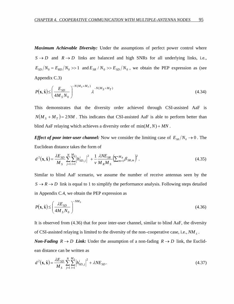
CHAPTER 4. COOPERATIVE COMMUNICATION WITH MULTIPLE-ANTENNA NODES 95
Maximum Achievable Diversity: Under the assumptions of perfect power control where
DS → and DR → links are balanced and high SNRs for all underlying links, i.e.,
100 >>= NENE RDSD and 00/ NENE SDSR >> , we obtain the PEP expression as (see
Appendix C.3)
( ))(
)(
04ˆ, TMSMN
MMN
S
SDTS
NME
P+
+−−
⎟⎟⎠
⎞⎜⎜⎝
⎛≤ λxx (4.34)
This demonstrates that the diversity order achieved through CSI-assisted AaF is
( ) NMMMN TS 2=+ . This indicates that CSI-assisted AaF is able to perform better than
blind AaF relaying which achieves a diversity order of MNNM +),min( .
Effect of poor inter-user channel: Now we consider the limiting case of 00 →NESR . The
Euclidean distance takes the form of
( ) ( )21 ,1 1
2,
2 1ˆ, ∑∑∑ == =
+= RS M
m mSRSR
SRN
j
M
i
ijSD
S
SD
MMNE
vh
ME
d βλλxx . (4.35)
Similar to blind AaF scenario, we assume the number of receive antennas seen by the
DRS →→ link is equal to 1 to simplify the performance analysis. Following steps detailed
in Appendix C.4, we obtain the PEP expression as
( )SNM
S
SD
NME
P−
⎟⎟⎠
⎞⎜⎜⎝
⎛≤
04ˆ,
λxx (4.36)
It is observed from (4.36) that for poor inter-user channel, similar to blind AaF, the diversity
of CSI-assisted relaying is limited to the diversity of the non–cooperative case, i.e., SNM .
Non-Fading DR → Link: Under the assumption of a non-fading DR → link, the Euclid-
ean distance can be written as
( ) SD
N
j
M
i
ijSD
S
SD NEhMEd
S
λλ+= ∑∑
= =1 1
2,
2 ˆ, xx . (4.37)
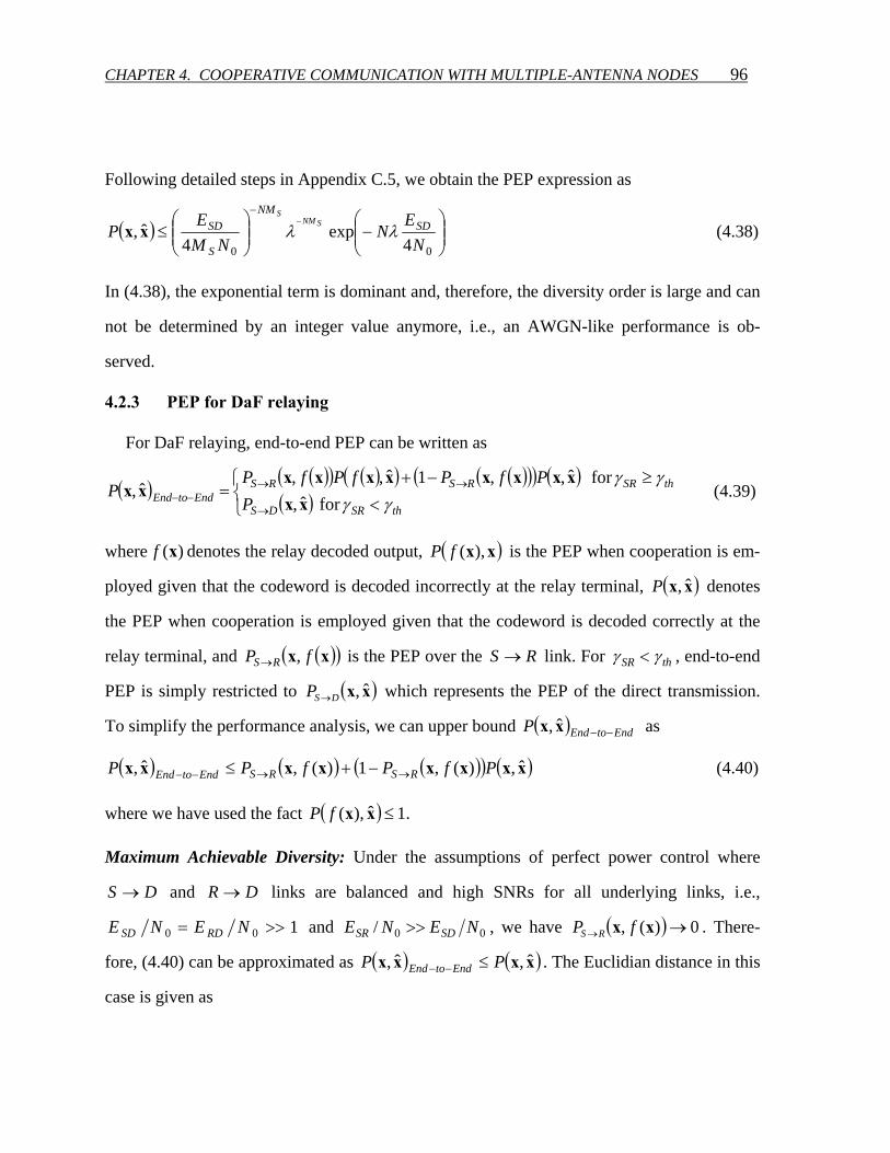
CHAPTER 4. COOPERATIVE COMMUNICATION WITH MULTIPLE-ANTENNA NODES 96
Following detailed steps in Appendix C.5, we obtain the PEP expression as
( ) ⎟⎟⎠
⎞⎜⎜⎝
⎛−⎟⎟
⎠
⎞⎜⎜⎝
⎛≤
−−
00 4exp
4ˆ,
NE
NNM
EP SD
NM
S
SD SNMS
λλxx (4.38)
In (4.38), the exponential term is dominant and, therefore, the diversity order is large and can
not be determined by an integer value anymore, i.e., an AWGN-like performance is ob-
served.
4.2.3 PEP for DaF relaying
For DaF relaying, end-to-end PEP can be written as
( ) ( )( ) ( )( ) ( )( )( ) ( )( )⎩
⎨⎧
<≥−+
=→
→→−−
thSRDS
thSRRSRSEndtoEnd P
PfPfPfPP
γγγγ
for ˆ,for ˆ,,1ˆ,,
ˆ,xx
xxxxxxxxxx (4.39)
where )(xf denotes the relay decoded output, ( )xx),(fP is the PEP when cooperation is em-
ployed given that the codeword is decoded incorrectly at the relay terminal, ( )xx ˆ,P denotes
the PEP when cooperation is employed given that the codeword is decoded correctly at the
relay terminal, and ( )( )xx fP RS ,→ is the PEP over the RS → link. For thSR γγ < , end-to-end
PEP is simply restricted to ( )xx ˆ,DSP → which represents the PEP of the direct transmission.
To simplify the performance analysis, we can upper bound ( ) EndtoEndP −−xx ˆ, as
( ) ( ) ( )( ) ( )xxxxxxxx ˆ,)(,1)(,ˆ, PfPfPP RSRSEndtoEnd →→−− −+≤ (4.40)
where we have used the fact ( ) .1ˆ),( ≤xxfP
Maximum Achievable Diversity: Under the assumptions of perfect power control where
DS → and DR → links are balanced and high SNRs for all underlying links, i.e.,
100 >>= NENE RDSD and 00/ NENE SDSR >> , we have ( ) 0)(, →→ xx fP RS . There-
fore, (4.40) can be approximated as ( ) ( )xxxx ˆ,ˆ, PP EndtoEnd ≤−− . The Euclidian distance in this
case is given as
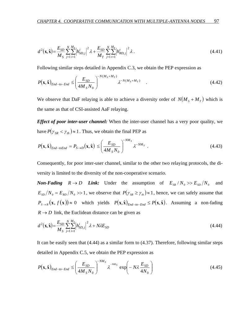
CHAPTER 4. COOPERATIVE COMMUNICATION WITH MULTIPLE-ANTENNA NODES 97
( ) ∑∑∑∑= == =
+=N
j
M
t
tjRD
T
SDN
j
M
i
ijSD
S
SD TS
hME
hME
d1 1
2,
1 1
2,
2 ˆ, λλxx . (4.41)
Following similar steps detailed in Appendix C.3, we obtain the PEP expression as
( ) )()(
04ˆ, TS
TSMMN
MMN
S
SDEndtoEnd NM
EP +−
+−
−− ⎟⎟⎠
⎞⎜⎜⎝
⎛≤ λxx . (4.42)
We observe that DaF relaying is able to achieve a diversity order of ( )TS MMN + which is
the same as that of CSI-assisted AaF relaying.
Effect of poor inter-user channel: When the inter-user channel has a very poor quality, we
have ( ) 1≈< thSRP γγ . Thus, we obtain the final PEP as
( ) ( )xxxx ˆ,ˆ, DStoEndEnd PP →− = S
SNM
NM
S
SD
NME −
−
⎟⎟⎠
⎞⎜⎜⎝
⎛≤ λ
04 . (4.43)
Consequently, for poor inter-user channel, similar to the other two relaying protocols, the di-
versity is limited to the diversity of the non-cooperative scenario.
Non-Fading DR → Link: Under the assumption of 00/ NENE SDSR >> and
100 >>= NENE RDSD , we observe that ( ) 1≈≥ thSRP γγ , hence, we can safely assume that
( )( ) 0, ≈→ xx fP RS which yields ( ) ( )xxxx ˆ,ˆ, PP EndtoEnd ≤−− . Assuming a non-fading
DR → link, the Euclidean distance can be given as
( ) SD
N
j
M
i
ijSD
S
SD ENhME
dS
λλ += ∑∑= =1 1
2,
2 ˆ,xx (4.44)
It can be easily seen that (4.44) as a similar form to (4.37). Therefore, following similar steps
detailed in Appendix C.5, we obtain the PEP expression as
( ) ⎟⎟⎠
⎞⎜⎜⎝
⎛−⎟⎟
⎠
⎞⎜⎜⎝
⎛≤
−−
−−00 4
exp4
ˆ,N
EN
NME
P SDNM
S
SDEndtoEnd
SNMS
λλxx (4.45)
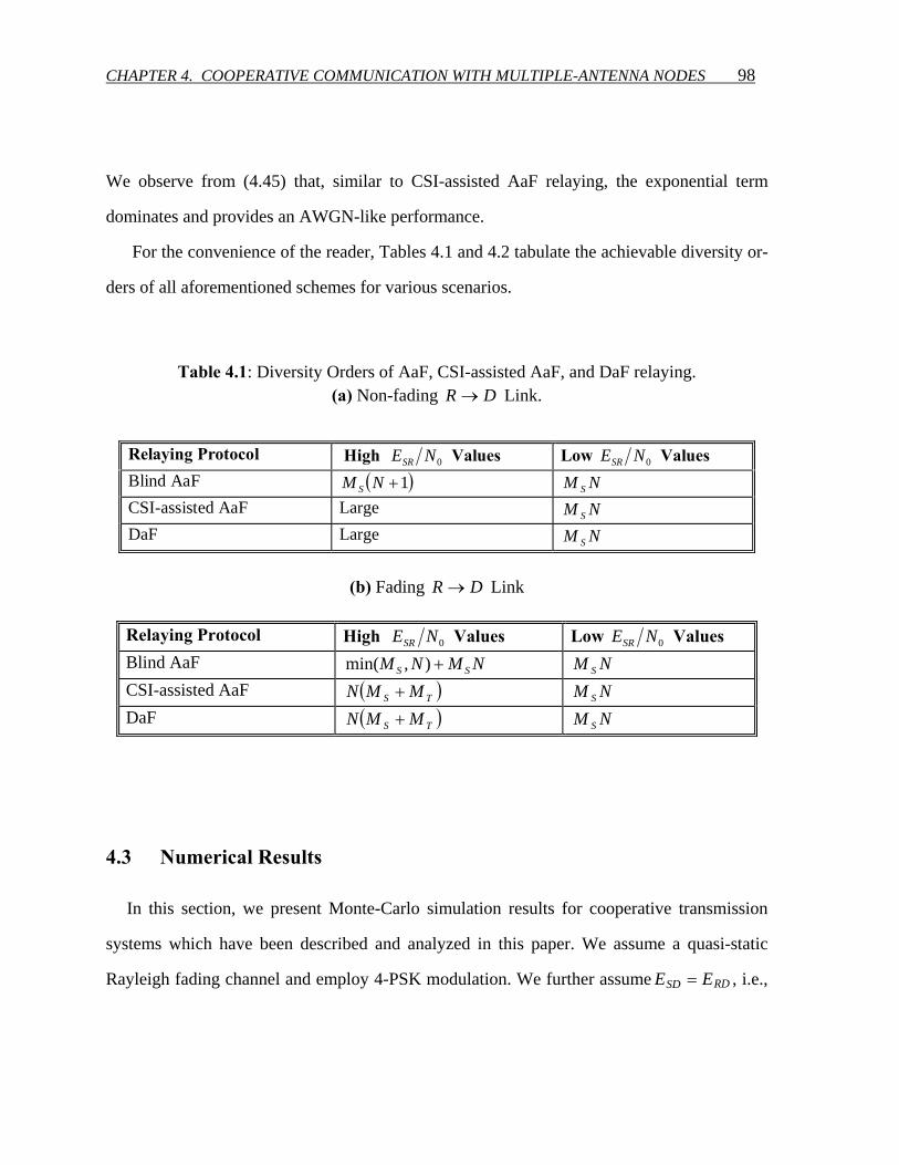
CHAPTER 4. COOPERATIVE COMMUNICATION WITH MULTIPLE-ANTENNA NODES 98
We observe from (4.45) that, similar to CSI-assisted AaF relaying, the exponential term
dominates and provides an AWGN-like performance.
For the convenience of the reader, Tables 4.1 and 4.2 tabulate the achievable diversity or-
ders of all aforementioned schemes for various scenarios.
Table 4.1: Diversity Orders of AaF, CSI-assisted AaF, and DaF relaying. (a) Non-fading DR → Link.
Relaying Protocol High 0NESR Values Low 0NESR Values Blind AaF ( )1+NM S NM S CSI-assisted AaF Large NM S DaF Large NM S
(b) Fading DR → Link
Relaying Protocol High 0NESR Values Low 0NESR Values Blind AaF NMNM SS +),min( NM S CSI-assisted AaF ( )TS MMN + NM S DaF ( )TS MMN + NM S
4.3 Numerical Results
In this section, we present Monte-Carlo simulation results for cooperative transmission
systems which have been described and analyzed in this paper. We assume a quasi-static
Rayleigh fading channel and employ 4-PSK modulation. We further assume RDSD EE = , i.e.,
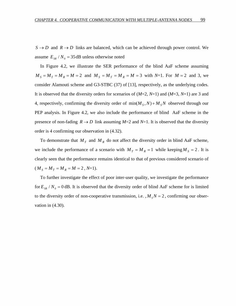
CHAPTER 4. COOPERATIVE COMMUNICATION WITH MULTIPLE-ANTENNA NODES 99
DS → and DR → links are balanced, which can be achieved through power control. We
assume 35/ 0 =NESR dB unless otherwise noted
In Figure 4.2, we illustrate the SER performance of the blind AaF scheme assuming
2==== MMMM RTS and 3==== MMMM RTS with N=1. For 2=M and 3, we
consider Alamouti scheme and G3-STBC (37) of [13], respectively, as the underlying codes.
It is observed that the diversity orders for scenarios of (M=2, N=1) and (M=3, N=1) are 3 and
4, respectively, confirming the diversity order of NMNM SS +),min( observed through our
PEP analysis. In Figure 4.2, we also include the performance of blind AaF scheme in the
presence of non-fading DR → link assuming M=2 and N=1. It is observed that the diversity
order is 4 confirming our observation in (4.32).
To demonstrate that TM and RM do not affect the diversity order in blind AaF scheme,
we include the performance of a scenario with 1== RT MM while keeping 2=SM . It is
clearly seen that the performance remains identical to that of previous considered scenario of
( 2==== MMMM RTS , N=1).
To further investigate the effect of poor inter-user quality, we investigate the performance
for 0/ 0 =NESR dB. It is observed that the diversity order of blind AaF scheme for is limited
to the diversity order of non-cooperative transmission, i.e. , 2=NM S , confirming our obser-
vation in (4.30).
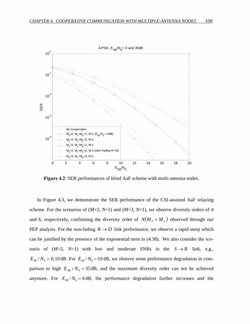
CHAPTER 4. COOPERATIVE COMMUNICATION WITH MULTIPLE-ANTENNA NODES 100
0 2 4 6 8 10 12 14 16 18 20
10-4
10-3
10-2
10-1
100
ESD/N0
SE
R
4-PSK, ESR/N0= 0 and 35dB
No CooperationMS=2, MT=MR=2, N=1 (ESR/N0 = 0dB)
MS=2, MT=MR=2, N=1
MS=2, MT=MR=1, N=1
MS=2, MT=MR=2, N=1 (Non-Fading R->D)
MS=3, MT=MR=3, N=1
Figure 4.2: SER performances of blind AaF scheme with multi-antenna nodes.
In Figure 4.3, we demonstrate the SER performance of the CSI-assisted AaF relaying
scheme. For the scenarios of (M=2, N=1) and (M=3, N=1), we observe diversity orders of 4
and 6, respectively, confirming the diversity order of ( )ST MMN + observed through our
PEP analysis. For the non-fading DR → link performance, we observe a rapid steep which
can be justified by the presence of the exponential term in (4.38). We also consider the sce-
nario of (M=2, N=1) with low and moderate SNRs in the RS → link, e.g.,
10 ,0/ 0 =NESR dB. For 10 / 0 =NESR dB, we observe some performance degradation in com-
parison to high 35/ 0 =NESR dB, and the maximum diversity order can not be achieved
anymore. For 0/ 0 =NESR dB, the performance degradation further increases and the
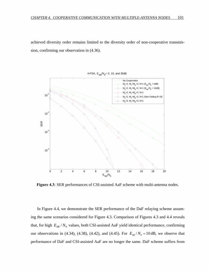
CHAPTER 4. COOPERATIVE COMMUNICATION WITH MULTIPLE-ANTENNA NODES 101
achieved diversity order remains limited to the diversity order of non-cooperative transmis-
sion, confirming our observation in (4.36).
0 2 4 6 8 10 12 14 16 18 20
10-4
10-3
10-2
10-1
ESD/N0
SE
R
4-PSK, ESR/N0= 0, 10, and 35dB
No CooperationM
S=2, M
T=M
R=2, N=1 (E
SR/N
0 = 0dB)
MS=2, M
T=M
R=2, N=1 (E
SR/N
0 = 10dB)
MS=2, M
T=M
R=2, N=1
MS=2, M
T=M
R=2, N=1 (Non-Fading R->D)
MS=3, M
T=M
R=3, N=1
Figure 4.3: SER performances of CSI-assisted AaF scheme with multi-antenna nodes.
In Figure 4.4, we demonstrate the SER performance of the DaF relaying scheme assum-
ing the same scenarios considered for Figure 4.3. Comparison of Figures 4.3 and 4.4 reveals
that, for high 0/ NESR values, both CSI-assisted AaF yield identical performance, confirming
our observations in (4.34), (4.38), (4.42), and (4.45). For 10/ 0 =NESR dB, we observe that
performance of DaF and CSI-assisted AaF are no longer the same. DaF scheme suffers from
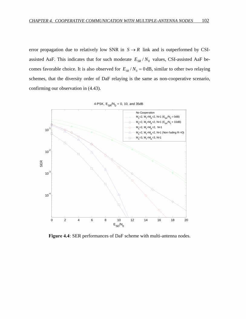
CHAPTER 4. COOPERATIVE COMMUNICATION WITH MULTIPLE-ANTENNA NODES 102
error propagation due to relatively low SNR in RS → link and is outperformed by CSI-
assisted AaF. This indicates that for such moderate 0/ NESR values, CSI-assisted AaF be-
comes favorable choice. It is also observed for 0/ 0 =NESR dB, similar to other two relaying
schemes, that the diversity order of DaF relaying is the same as non-cooperative scenario,
confirming our observation in (4.43).
0 2 4 6 8 10 12 14 16 18 20
10-4
10-3
10-2
10-1
ESD/N0
SE
R
4-PSK, ESR/N0 = 0, 10, and 35dB
No CooperationMS=2, MT=MR=2, N=1 (ESR/N0 = 0dB)
MS=2, MT=MR=2, N=1 (ESR/N0 = 10dB)
MS=2, MT=MR=2, N=1
MS=2, MT=MR=2, N=1 (Non-fading R->D)
MS=3, MT=MR=3, N=1
Figure 4.4: SER performances of DaF scheme with multi-antenna nodes.
CHAPTER 4. COOPERATIVE COMMUNICATION WITH MULTIPLE-ANTENNA NODES 103
Appendix C
C.1 Derivation of Eqs. (4.25)-(4.26)-(4.27)
In this Appendix, we derive the PEP expression for blind AaF scheme assuming fading
DR → link. The Euclidean distance ( )xx ˆ,2d is given by (4.23) and repeated here for con-
venience
( ) ( ) ( )xxxxxx ˆ,ˆ,ˆ, 222DSDRS ddd →→→ +=
∑∑∑∑= ===
+=N
j
M
i
ijSD
S
SDM
i
iSR
N
jjRDjTR
SS
hMEhhMM
1 1
2,
1
2
1
2,
λωλ . (4.46)
For the asymptotic case of 100 >>= NENE RDSD with perfect power control and suffi-
ciently large 00/ NENE SDSR >> values, jω can be approximated as ./1 TRSj MMM≈ω
Therefore, (4.46) reduces to
∑∑ ∑∑= = ==
+=N
j
M
i
M
i
iSR
N
jjRD
S
SDijSD
S
SDS S
hhME
hME
d1 1 1
2
1
2,
2,
2 )ˆ(λλ
xx, . (4.47)
Introducing ∑ ∑= == Nj
Mi
ijSD
S hY 1 1
2,1 and 212 ZZY = with ∑ == N
j jRDhZ 12
,1 and
∑ == SMi
iSRhZ 1
22 , we can rewrite (4.47) as
( ) 212 ˆ, Y
MEY
MEd
S
SD
S
SD λλ+=xx . (4.48)
After substituting (4.48) in (4.22), we have the PEP expression as
⎟⎟⎠
⎞⎜⎜⎝
⎛−⎟⎟
⎠
⎞⎜⎜⎝
⎛−≤ 2
01
021 4
exp4
exp),|ˆ,( YMN
EY
MNE
YYPS
SD
S
SD λλxx (4.49)
The unconditional PEP can be obtained as [84]
( ) ( ) ( )0
2
0
14
4
ˆ,
NMEjY
NMEjY
S
SD
S
SDP λω
λω
ωω−=−=
Φ×Φ≤xx (4.50)
where ( )ω1YΦ and ( )ω2YΦ are the characteristic functions of 1Y and 2Y , respectively. Since i
jSDh , is Rayleigh distributed, the characteristic function of 1Y can be readily found as [84]
CHAPTER 4. COOPERATIVE COMMUNICATION WITH MULTIPLE-ANTENNA NODES 104
NM
S
SD
MjY
S
SNM
E−
−= ⎟⎟⎠
⎞⎜⎜⎝
⎛+=Φ λω λω
4
1) (0N4
E 0
SD1. (4.51)
where the first term can be further ignored under high SNR assumption. In the following, we
will derive the PEP expression under three different scenarios:
Case 1 ( SMN > ): The characteristic function of Y2 can evaluated as [85]
∫∞
Φ=Φ0
112112 ) ()()( dzzzf ZZY ωω , (4.52)
where )( 11zfZ is the pdf of 1Z and ) ( 12 zZ ωΦ has the similar form as in (4.51). Here, 1z is a
chi-squared random variable with N2 degrees of freedom with the pdf
( )Nezzf zNZ Γ= −− 1
1
111)( , 0 1 ≥z [86] where ( ).Γ denotes the gamma function [71]. This
leads to
( ) ∫∞
−−−
−−
−= ⎟⎟⎠
⎞⎜⎜⎝
⎛+⎟⎟
⎠
⎞⎜⎜⎝
⎛Γ
=Φ0
11
110
04E
1
0
SD2
44
1)( dzezzE
NMNM
EN
zNM
SD
SMM
S
SD
NMjY
S
S
S
Sλ
λω λω
, (4.53)
Assuming high SNR, i.e., 04NESD >>1 and using the integral form given by [71, p.382,
3.351.3], we obtain
( )( )
S
S
S
MM
S
SDS
NMjY NM
ENMN −
−
−= ⎟⎟⎠
⎞⎜⎜⎝
⎛Γ−Γ
=Φ λω λω
04E 4
)(0
SD2 (4.54)
Substituting (4.54) and (4.51) in (4.50), we find the final PEP expression as
( ) ( )( )
)1(
0
)1(
4ˆ,
+−+−
⎟⎟⎠
⎞⎜⎜⎝
⎛Γ
−Γ≤
NM
S
SDNM
SSS
NME
NMN
Pλ
xx (4.55)
Case 2 ( NM S > ): Noting that this case is similar to the previous case with N and SM now
interchanged, we follow similar steps and find the PEP expression as
( ) ( )( )
)1(
0
)1(
4ˆ,
+−+−
⎟⎟⎠
⎞⎜⎜⎝
⎛Γ−Γ
≤SS
MN
S
SD
S
MNS
NME
MNMP λxx (4.56)
CHAPTER 4. COOPERATIVE COMMUNICATION WITH MULTIPLE-ANTENNA NODES 105
Case 3 ( NM S = ): Following the same argument in Case 1 and further defining 1 zu +=υ ,
where ( )SDS ENM λυ /4 0= , we write (4.53) as
0
SD24
E )(
NMjY
S
λω
ω−=
Φ ( ) ( ) ( )∫∞
−−−−−
−⎟⎟⎠
⎞⎜⎜⎝
⎛Γ
=υ
υυλ dueuuNM
EN
uNMM
S
SD S
S11
0/1exp
41 (4.57)
Under 04NESD >>1 assumption, 1/1 ≈− uυ , we can rewrite (4.57) as
( ) ( ) ( )υυλω λω
,0exp4
1)(04
E 0
SD2Γ⎟⎟
⎠
⎞⎜⎜⎝
⎛Γ
=Φ −−
−=S
S
S
MM
S
SD
NMjY NM
EN
(4.58)
Using the limiting approximation ( )υυ log),0( −≈Γ for 0→υ [71], (4.58) further reduces to
( ) ⎟⎟⎠
⎞⎜⎜⎝
⎛⎟⎟⎠
⎞⎜⎜⎝
⎛Γ
=Φ −−
−=004
E log
41)(
0
SD2 NE
NME
NSDM
M
S
SD
NMjY
S
S
S
λω λω
(4.59)
Substituting (4.59) and (4.51) in (4.50), we find the final PEP expression as
( ) ( )
)1(
00
)1(
4logˆ,
+−+−
⎟⎟⎠
⎞⎜⎜⎝
⎛⎟⎟⎠
⎞⎜⎜⎝
⎛Γ
≤NM
S
SDSDNM SS
NME
NE
NP λxx (4.60)
C.2 Derivation of Eq. (4.30)
In this Appendix, we derive the PEP expression for blind AaF relaying scheme assuming the
limiting case of 00 →NESR . Under this scenario, )ˆ(2 xx,d is given as (4.29) where 1Y and
2Y are now defined by ∑ ∑= == Nj
Mi
ijSD
S hY 1 1
2,1 and ∑ == SM
ii
SRhY 1
22 . Since i
jSDh , and iSRh are
Rayleigh distributed, their characteristic functions are readily available (See Eq. (4.51)). Re-
placing those in (4.50), we find the PEP as
SS M
S
SRNM
S
SD
NME
NME
P−−
⎟⎟⎠
⎞⎜⎜⎝
⎛+⎟⎟
⎠
⎞⎜⎜⎝
⎛≤ λλ
00 41
4)ˆ,( xx (4.61)
CHAPTER 4. COOPERATIVE COMMUNICATION WITH MULTIPLE-ANTENNA NODES 106
C.3 Derivation of Eq. (4.34)
In this Appendix, we derive the PEP expression for the CSI-assisted AaF relaying scheme
assuming a fading DR → link. In this case, )ˆ(2 xx,d is given as
( )xx ˆ,2d ( )21 ,1
2,
11 1
2, ∑∑∑∑∑ =
=== =+= R
TS Mm mSR
M
m
mjRD
N
jj
N
j
M
i
ijSD
S
SD hhME βαλ
λ (4.62)
Under the assumption of 100 >>= NENE RDSD with perfect power control and sufficiently
large 00/ NENE SDSR >> values, the scaling factor in (4.19) reduces to
( ) 121 ,
−
= ⎟⎠⎞⎜
⎝⎛= ∑ RM
m mSRTSDj ME βα . Hence, (4.62) is simplified as
( ) ∑∑∑∑= == =
+=N
j
M
m
mjRD
T
SDN
j
M
i
ijSD
S
SDTS
hME
hME
d1 1
2,
1 1
2,
2 ˆ,λλ
xx (4.63)
(4.63) can be written in the same form as (4.48) where 1Y and 2Y are now defined by
∑ ∑= == Nj
Mi
ijSD
S hY 1 1
2,1 and ∑ ∑= == N
jMm
mjRD
T hY 1 1
2,2 . Since i
jSDh , and iSRh are Rayleigh dis-
tributed, their characteristic functions are readily available. c.f., (4.51). Replacing those in
(4.50), we find the PEP as
( ))(
)(
04ˆ, TMSMN
MMN
S
SDTS
NMEP
++−
−
⎟⎟⎠
⎞⎜⎜⎝
⎛≤ λxx (4.64)
C.4 Derivation of Eq. (4.36)
In this Appendix, we derive the PEP expression for the CSI-assisted AaF relaying scheme
assuming the limiting case of 00 →NESR . Under this scenario, )ˆ(2 xx,d is given by (4.35).
Substituting (4.35) in (4.22), we find the PEP expression as
CHAPTER 4. COOPERATIVE COMMUNICATION WITH MULTIPLE-ANTENNA NODES 107
( )⎥⎥⎦
⎤
⎢⎢⎣
⎡⎟⎟⎠
⎞⎜⎜⎝
⎛−≤ ∑∑
= =
N
j
M
i
ijSD
S
SD
h
S
ijSD
hNM
EP
1 1
2,
04expEˆ,
,
λxx
( )4444444444 34444444444 21
κ
ββλ
⎥⎥⎦
⎤
⎢⎢⎣
⎡⎟⎟⎠
⎞⎜⎜⎝
⎛∑−× =
→
21 ,
00/ 41expElim
,0
R
mSRSR
Mm mSR
SR
SRNE NE
MMN
v (4.65)
For the limiting case of 00 →NESR , it can be easily noticed that 1→κ . Therefore, the first
term in this case evidently dominates the performance. Performing the expectation with re-
spect to ijSDh , , which is Rayleigh distributed, PEP is found as
( )SNM
S
SD
NME
P−
⎟⎟⎠
⎞⎜⎜⎝
⎛≤
04ˆ,
λxx (4.66)
C.5 Derivation of Eq. (4.38)
In this Appendix, we derive the PEP expression for the CSI-assisted AaF relaying under the
assumption of a non-fading DR → link. Replacing ( )21 ,1 ∑ == RMm mSRTj M βα in (4.33), we
have
( ) SD
N
j
M
i
ijSD
S
SD NEhMEd
S
λλ
+= ∑∑= =1 1
2,
2 ˆ,xx . (4.67)
Substituting (4.67) in (4.22) and taking the expectation with respect to ijSDh , which is
Rayleigh distributed, we find PEP as
( ) ⎟⎟⎠
⎞⎜⎜⎝
⎛−⎟⎟
⎠
⎞⎜⎜⎝
⎛≤
−−
00 4exp
4ˆ,
NE
NNM
EP SD
NM
S
SD SNMS
λλxx (4.68)
108
Chapter 5
Conclusions and Future Work
Introduction
In this final chapter, we summarize the contributions of the work presented in this disser-
tation and discuss several potential extensions to our work.
5.1 Research Contributions
Cooperative networks have recently attracted much attention and fundamental informa-
tion-theoretic aspects of these networks have been already well documented. However, prac-
tical implementation of cooperative communication requires an in-depth investigation of sev-
eral physical layer issues such as channel estimation and equalization integrating the underly-
ing cooperation protocols and relaying modes. In this dissertation, we have designed and ana-
lyzed equalization and channel estimation schemes for cooperative communication and fur-
ther investigated the deployment of multiple-antennas in cooperative networks. In further
detail, we summarize our conclusions and main findings of this dissertation as follows:
In Chapter 2, we have proposed and analyzed time-domain and frequency-domain equali-
zation for cooperative communication. The considered schemes D-TR-STBC, D-SC-STBC
and D-OFDM-STBC are built upon the distributed implementation of STBCs with AaF re-
CHAPTER 5 CONCLUSIONS AND FUTURE WORK 109
laying and allow low-complexity designs due to the underlying orthogonality of the code.
Through PEP derivations, we have presented a diversity gain analysis for the three equaliza-
tion schemes under consideration. Under the assumption of perfect power control for the re-
lay terminal and high SNR for the underlying links, we have demonstrated that D-TR-STBC
and D-SC-STBC schemes yield identical performance achieving a maximum diversity order
of 221 ++ LL for a non-fading DR → link and 223 ++ LL for a non-fading RS → link,
where L1, L2, and L3 are the channel memory lengths for RS → , DS → and DR → links,
respectively. For the general case where all underlying links experience frequency selectivity,
these two schemes achieve a diversity order of ( ) 2,min 231 ++ LLL . Under the same assump-
tions, the uncoded D-OFDM-STBC scheme achieves only a maximum diversity order of two
since it is not able to exploit the underlying multipath diversity. However, by combining D-
OFDM-STBC scheme with interleaving and a judiciously-designed outer code, we have
demonstrated that it is able to provide the same diversity of D-TR-STBC and D-SC-STBC.
In Chapter 3, we have investigated non-coherent and mismatched-coherent receivers for
distributed STBC operating in AaF relaying mode. First, we have studied ML sequence esti-
mation for the distributed STBC scheme without assuming channel knowledge. Under quasi-
static fading assumption, we have shown that the ML rule reduces to a simple form due to the
orthogonality structure of STBC which allows us to develop a recursive expression. Through
the PEP analysis, we have demonstrated that the proposed decoder achieves full diversity. As
an alternative scheme, we have considered the mismatched-coherent receiver where channel
estimation is carried through pilot symbols. We have demonstrated through PEP analysis that
the mismatched-coherent receiver is able to collect the full diversity as its non-coherent com-
petitor over quasi-static channels. We have further presented a comprehensive comparison of
two competing schemes under various mobility scenarios.
CHAPTER 5 CONCLUSIONS AND FUTURE WORK 110
In Chapter 4, we have investigated the effect of multiple antenna deployment assuming
different relaying techniques. In particular, we have investigated the error rate performance
of blind AaF, CSI-assisted AaF, and DaF schemes in a single-relay assisted transmission
scenario where the source, relay, and destination terminals are equipped with SM ,
RT MM = , and N antennas, respectively. Under the assumption of perfect power control for
the relay terminal and high SNR for the underlying links, we have shown through the PEP
analysis that the maximum diversity order is NMNM SS +),min( for the underlying blind
AaF scheme and ( )ST MMN + for both CSI-assisted AaF and DaF schemes. For the case of
a non-fading DR → link, we have demonstrated that the considered blind AaF scheme is
able to achieve a diversity order of ( )1+NM S . On the other hand, the maximum diversity
order of CSI-assisted AaF and DaF schemes is large and can not be determined by an integer
value.
5.2 Future Work
While several key results for cooperative communication have been reported in this dis-
sertation, there are several possible research topics yet to be explored as extensions of the
current work.
Our results in Chapter 2 are mainly limited to single-relay deployment. While we believe
that our results can be extended in a straightforward manner to the general case of multiple
relays through the deployment of G3, G4, H3, H4 STBCs [13] in a distributed fashion, fur-
ther investigation is required to characterize how the diversity orders interact. It is also well
known that space-time codes (conventional ones as well as their distributed versions) suffer a
loss in throughput efficiency for more than two transmit antennas. To address transmission
rate efficiency, so-called quasi-orthogonal STBCs (QO-STBCs) has been proposed in [101].
In QO-STBC, the orthogonality assumption is relaxed to achieve full transmission rate. In
CHAPTER 5 CONCLUSIONS AND FUTURE WORK 111
[40], we have investigated time-domain equalization for QO-STBC over frequency-selective
channels, exploiting the embedded quasi-orthogonal structure to design low-complexity re-
ceivers. Further application of QO-STBC to cooperative communication scheme still remains
an interesting open problem. It would also be interesting to examine the performance for
other fading distributions, such as Ricean and Nakagami fading.
In Chapter 2 of this dissertation, our performance analysis has assumed MLSE equaliza-
tion although we did investigate the performance of MMSE equalizers via Monte-Carlo
simulation. The complexity of MLSE equalizers is prohibitive for many applications particu-
larly for long channel impulse responses and high order modulation. It would be of practical
importance to investigate suboptimal techniques such as Zero-Forcing (ZF) [86], MMSE
[86], and decision feedback (DF) [86] equalizers in the context of cooperative communica-
tion.
A key underlying assumption in this dissertation is that the cooperating terminals trans-
mit with same power, i.e., equal power allocation. To improve overall performance and in-
crease energy efficiency, the following two questions need to be addressed: 1) How much
overall power should be shared between broadcasting and relaying phases?, 2) How much
power should be allocated to relay-to-destination and source-to-destination links in the relay-
ing phase? Recent results have shown that the performance of cooperative networks can be
substantially improved by optimally distributing the power among cooperating terminals
[99], [100]. However, the current results are mainly restricted to frequency-flat channels.
Thus, a rich area for future research would be to investigate optimal power allocation rules
for D-TR-STBC, D-SC-STBC, and D-OFDM-STBC schemes.
In Chapter 3, we have exploited the orthogonal structure of distributed STBCs to derive a
non-coherent decoding rule which can be implemented in practice by a Viterbi-type algo-
rithm. However, we have only considered Alamouti code which requires a single relay node
CHAPTER 5 CONCLUSIONS AND FUTURE WORK 112
deployment, i.e., STBC designed for two transmit antennas [15]. Extension to multiple
relays, design of a channel estimator without the imposed orthogonality assumption, and
differential detection are possible further research areas on this topic. As for mismatched-
coherent detection, there are several issues that can be addressed in the context of cooperative
communication. For example, since for channel estimation purposes, pilot symbols are em-
ployed, there is a need for an optimal design. Recently, for non-cooperative scenarios, few
results have emerged, which suggest that significant potential gain can be realized if pilot
symbols are designed optimally and placed judiciously [102]-[105]. It is an open research
question to determine the number of pilot symbols, the power allocated for pilot symbols,
and the locations of these pilots for cooperative networks taking into account the relay loca-
tion and relaying technique.
In chapter 4, we have analyzed the effects of multiple-antenna deployment over fre-
quency flat fading channels. A potential future research area is to investigate multiple an-
tenna deployment in broadband cooperative networks over frequency-selective channels and
further consider the problem of power allocation for such a scenario.
113
Bibliography
[1] S. Y. Hui and K. H. Yeung, “Challenges in the Migration to 4G Mobile Systems,” IEEE Commun. Mag., vol. 41, pp. 54 - 59, December 2003
[2] T. S. Rappaport, Wireless Communications: Principles and Practice, Prentice Hall PTR, 2000.
[3] W. C. Jakes, Microwave Mobile Communications, New York: Wiley, 1974.
[4] D. Tse and P. Viswanath, Fundamentals of Wireless Communication, Cambridge University Press, 2005.
[5] A. Wittneben, “Base station modulation diversity for digital SIMULCAST,” in Pro-ceedings of the IEEE Vehicular Technology Conference (VTC), pp. 848-853, May 1991.
[6] A. Wittneben, “A new bandwidth efficient transmit antenna modulation diversity scheme for linear digital modulation,” in Proceedings of the IEEE International Conference Communications (ICC), pp. 1630-1634, May 1993.
[7] J. H. Winters, “Diversity gain of transmit diversity in wireless systems with Rayleigh fading,” IEEE Trans. Veh. Technol., vol. 47, pp. 119-123, February 1998.
[8] V. Tarokh, N. Seshadri, and A.R. Calderbank, “Space-time codes for high data rates wireless communications: Performance criterion and code construction,” IEEE Trans. Inf. Theory, vol. 44, pp. 744-765, 1998.
[9] J. G. Foschini, “Layered space-time architecture for wireless communication in a fading environment when using multi element antennas,” Bell Labs Tech. J., vol. 2, pp. 41-59, Autumn 1996.
[10] C. Kose and R. D. Wesel, “Universal space-time trellis codes,” IEEE Trans. Inf. Theory, vol. 49, pp. 2717-2727, Oct. 2003.
[11] Z. Safar and K. J. R. Liu, “Systematic space-time trellis code construction for corre-lated Rayleigh-fading channels,” IEEE Trans. Inf. Theory, vol. 50, pp. 2855-2865, Nov. 2004.
BIBLIOGRAPHY
114
[12] L. Yonghui, B. Vucetic, Y. Tang, and Q. Zhang, “Space-time trellis codes with lin-ear transformation for fast fading channels,” IEEE Signal Process. Lett., vol. 11, no. 11, pp. 895- 898, Nov. 2004.
[13] V. Tarokh, H. Jafarkhani, and A.R. Calderbank, “Space-time block coding from or-thogonal designs,” IEEE Trans. Inf. Theory, vol. 45, pp. 1456-1467, 1999.
[14] V. Tarokh, H. Jafarkhani, and A.R. Calderbank, “Space-time block coding for wire-less communications: Performance results,” IEEE J. Sel. Areas Commun., vol. 17, pp. 451-460, 1999.1
[15] S. M. Alamouti, “Simple transmit diversity technique for wireless communications,” IEEE J. Sel. Areas Commun., vol. 16, pp. 1451-1458, 1998.
[16] H. Wang and X.-G. Xia, “Upper bounds of rates of complex orthogonal space-time block codes,” IEEE Trans. Inf. Theory, vol. 49, no. 10, pp. 2788–2796, October 2003.
[17] S. Das, N. Al-Dhahir, and R. Calderbank, “Novel full-diversity high-rate STBC for 2 and 4 transmit antennas,” IEEE Commun. Lett., vol. 10, no. 3, pp. 171-173, March 2006.
[18] H. Jafarkhani and N. Seshadri, “Super-orthogonal space-time trellis codes”, IEEE Trans. Inf. Theory, vol. 49, no. 4 , pp. 937-950, April 2003.
[19] B. Hassibi and B. Hochwald, “High-rate codes that are linear in space and time”, IEEE Trans. Inf. Theory, vol. 48, no. 7 , pp. 1804-1824, July 2002.
[20] R. W. Heath and A. Paulraj, “Linear dispersion codes for MIMO Systems based on frame theory,” IEEE Trans. Signal Process., vol. 50, no. 10, 2429-2441, October 2002.
[21] B. Vucetic and J. Yuan, Space-Time Coding, John Wiley & Sons, May 2003.
[22] A. Paulraj, D. Gore and R. Nabar, Introduction to Space-Time Wireless Communications, Cambridge University Press, May 2003
[23] H. Jafarkhani, Space-Time Coding: Theory and Practice, Cambridge University Press, September 2005.
[24] A. Sendonaris, E. Erkip, and B. Aazhang, “User Cooperation Diversity – Part I: Sys-tem Description,” IEEE Trans. Commun., vol. 51, pp. 1927-1938, Nov. 2003.
[25] A. Sendonaris, E. Erkip, and B. Aazhang, “User Cooperation Diversity – Part II: Implementation, Aspects and Performance Analysis,” IEEE Trans. Commun., vol. 51, pp 1939-1948, Nov. 2003
BIBLIOGRAPHY
115
[26] J. N. Laneman, D. N. C. Tse, and G. W. Wornell, “Cooperative Diversity in Wire-less Networks: Efficient Protocols and Outage Behavior,” IEEE Trans. Inf. Theory, vol. 50, no. 12, pp. 3062-3080, Dec. 2004.
[27] J. N. Laneman, G. W. Wornell, and D. N. C. Tse, “An Efficient Protocol for Realiz-ing Cooperative Diversity in Wireless Networks,” in Proceedings of the IEEE Inter-national Symposium on Information Theory (ISIT), Washington, DC, June 2001.
[28] J. N. Laneman and G. W. Wornell, “Distributed Space-Time Coded Protocols for Exploiting Cooperative Diversity in Wireless Networks,” IEEE Trans. Inf. Theory, vol. 49, no. 10, pp. 2415-2525, Oct. 2003.
[29] E. V. D. Meulen, “Three-terminal communication channels,” Advances in Applied Probability, vol. 3, pp. 120-154, 1971.
[30] T. M. Cover and A. A. El Gamal. “Capacity theorems for the relay channel,” IEEE Trans. Inf. Theory, vol. 25, pp. 572-584, Sept. 1979.
[31] T. E. Hunter and Aria Nosratinia, “Cooperation diversity through coding” in Pro-ceedings of the IEEE International Symposium on Information Theory (ISIT), Lausanne, Switzerland, June 2002.
[32] T. E. Hunter and Aria Nosratinia, “Diversity through coded cooperation,” IEEE Trans. Wireless Commun., vol. 5, no. 2, pp. 283-289, Feb. 2006.
[33] R. U. Nabar, H. Bölcskei, and F. W. Kneubühler, “Fading relay channels: Perform-ance limits and space-time signal design”, IEEE J. Sel. Areas Commun., vol. 22, no. 6, pp. 1099-1109, August 2004.
[34] K. Azarian, H. El Gamal, and P. Schniter, “On the achievable diversity multiplexing tradeoff in half-duplex cooperative channels,” IEEE Trans. Inf. Theory, vol. 51, pp. 4152–4172, Dec. 2005.
[35] N. Al-Dhahir, “Single Carrier Frequency Domain Equalization for Space Time Block Coded Transmissions over Frequency Selective Fading Channels,” IEEE Commun. Lett., vol. 5, no. 7, pp. 304-306, July 2001.
[36] Z. Liu, G. B. Giannakis, A. Scaglione, and S. Barbarossa, “Block Precoding and Transmit-Antenna Diversity for Decoding and Equalization of Unknown Multipath Channels,” in Proceedings of the of 33rd Asilomar Conference Signals, Systems, and Computers, Nov. 1999
[37] E. Lindskog and A. Paulraj, “A Transmit Diversity Scheme for Channel with ISI,” in Proceedings of the International Conference on Communications (ICC), June 2000.
BIBLIOGRAPHY
116
[38] H. Mheidat, M. Uysal and N. Al-Dhahir, “Comparative Analysis of Equalization Techniques for STBC with Application to EDGE”, in Proceedings of the IEEE Ve-hicular Technology Conference (VTC), Milano, Italy, May 2004.
[39] H. Mheidat, M. Uysal and N. Al-Dhahir, “Time-and Frequency-Domain Equaliza-tion for Quasi-Orthogonal STBC over Frequency-Selective Channels”, in Proceed-ings of the International Conference on Communications (ICC), Paris, France, July 2004.
[40] H. Mheidat, M. Uysal, and N. Al-Dhahir, “Quasi-Orthogonal Time-Reversal Space-Time Block Coding for Frequency-Selective Fading Channels”, to appear in IEEE Trans. Signal Process.
[41] S. Yatawatta and A. P. Petropulu, “ A Multi-user OFDM System with User Coop-eration,” 38th Asilomar Conference on Signals, Systems, and Computers, Nov. 2004.
[42] P. A. Anghel and M. Kaveh, “Exact symbol error probability of a Cooperative net-work in a Rayleigh-fading environment”, IEEE Trans. Wireless Commun., vol. 3, no. 5, p. 1416 – 1421, Sept. 2004
[43] P. A. Anghel and M. Kaveh, “Relay assisted uplink communication over frequency-selective channels”, in Proceedings of the 4th IEEE Workshop on Signal Process-ing Advances in Wireless Communications (SPAWC), June, 2003.
[44] X. Li, F. Ng, J. Hwu and M. Chen, "Channel equalization for STBC-encoded coop-erative transmissions with asynchronous transmitters," in Proceedings of the 39th Asilomar Conference on Signals, Systems and Computers, Pacific Grove, CA, Oct. 30-Nov. 2, 2005.
[45] G. Scutari and S. Barbarossa, “Distributed Space–Time Coding for Regenerative Relay Networks,” IEEE Trans. Wireless Commun., vol. 4, no. 5, pp.2387-2399, September 2005
[46] H. Mheidat, M. Uysal, and N. Al-Dhahir, “Equalization Techniques for Distributed Space-Time Block Codes with Amplify-and-Forward Relaying”, accepted for publi-cation in IEEE Trans. Signal Process.
[47] H. Mheidat, M. Uysal, and N. Al-Dhahir, “Equalization Techniques for Space-Time Coded Cooperative Systems”, in Proceedings of the IEEE Vehicular Technology Conference (VTC), Los Angeles, California, USA, September 2004.
[48] H. Mheidat, M. Uysal, and N. Al-Dhahir, “Distributed Space-Time Block Coded OFDM for Relay-Assisted Transmission”, in Proceedings of the IEEE International Conference on Communications (ICC), Istanbul, Turkey, June 2006.
BIBLIOGRAPHY
117
[49] H. Mheidat, M. Uysal, and N. Al-Dhahir, “Time-Reversal Space-Time Equalization for Amplify-and-Forward Relaying”, in Proceedings of the IEEE International Con-ference on Communications (ICC), Istanbul, Turkey, June 2006.
[50] H. Mheidat, M. Uysal, and N. Al-Dhahir, “Single-Carrier Frequency Domain Equalization for Broadband Cooperative Communications”, in Proceedings of the IEEE Wireless Communications and Networking Conference (WCNC), Las Vegas, Nevada, USA, April 2006.
[51] D. Chen and J. N. Laneman, “Non-coherent Demodulation for Cooperative Wireless Systems,” in Proceedings of the IEEE Global Telecommunications Conference (GLOBECOM), Dallas, TX, Nov. 2004
[52] P. Tarasak, H. Minn, and V.K. Bhargava, “Differential Modulation for Two-User Cooperative Diversity Systems,” IEEE J-SAC: Differential and Non coherent Wire-less Communications, vol. 23, no. 9, pp. 1891-1900, Sept. 2005
[53] T. Wang, Y. Yao, and G. B. Giannakis, “Non-Coherent Distributed Space-Time Processing for Multiuser Cooperative Transmissions,” in Proceedings of the IEEE Global Telecommunications Conference (GLOBECOM), St. Louis, December 2005
[54] S. Yiu, R. Schober, and L. Lampe, “Distributed Space-Time Block Coding,” IEEE Trans. Commun., vol. 54, no.7, pp.1195-1206, July 2006.
[55] S. Yiu, R. Schober, and L. Lampe, “Non-coherent Distributed Space-Time Block Coding,” in Proceedings of the IEEE Vehicular Technology Conference (VTC), Dal-las, USA, September 2005.
[56] R. Annavajjala, P. Cosman, and L. Milstein, “On the Performance of Optimum Non-coherent Amplify-and-Forward Reception for Cooperative Diversity,” IEEE Military Communications Conference (MILCOM 2005), Atlantic City, USA, Oct. 2005.
[57] H. Mheidat and M. Uysal, “Non-Coherent and Mismatched-Coherent Receivers for Distributed STBCs with Amplify-and-Forward Relaying”, under second round re-view in IEEE Trans. Wireless Commun.
[58] M. Uysal and H. Mheidat, “Maximum-Likelihood Detection for Distributed Space-Time Block Coding”, ,” in Proceedings of the IEEE Vehicular Technology Confer-ence (VTC), Los Angeles, California, USA, September 2004.
[59] P. Gupta and P. R. Kumar, “The capacity of wireless networks,” IEEE Trans. Inf. Theory, vol. 46, pp. 388–404, Mar. 2002.
[60] M. Gastpar and M. Vetterli, “On the capacity of wireless networks: The relay case,” in Proceedings of the IEEE INFOCOM, New York, USA, June 2002.
BIBLIOGRAPHY
118
[61] R. Pabst, B. H. Walke, D. C. Schultz, P. Herhold, H. Yanikomeroglu, S. Mukher-jeee, H. Viswanathan, M. Lott, W. Zirwas, M. Dohler, H. Aghvami, D. D. Falconer, and G. P. Fettweis, “Relay-based deployment concepts for wireless and mobile broadband radio,” IEEE Commun. Mag., vol. 42, no. 9, pp. 80–89, Sep. 2004.
[62] P. Gupta, P.R. Kumar, “Towards an Information Theory of Large Networks: An Achievable Rate Region,” IEEE Trans. Inf. Theory, vol. 49, pp. 1877-1894, August 2003.
[63] B. Wang, J. Zhang and A. Host-Madsen, “On the Capacity of MIMO Relay Chan-nels,” IEEE Trans. Inf. Theory, vol. 51, no. 1, pp. 29-43, Jan. 2005.
[64] Y. Jing B. Hassibi, “Cooperative Diversity in Wireless Relay Networks with Multi-ple-Antenna Nodes”, in IEEE International Symposium on Information Theory (ISIT), pp. 815 – 819, September 2005.
[65] S. Yiu and R. Schober, “On Distributed Space-Time Filtering,” in Proceedings of the IEEE Global Telecommunications Conference (GLOBECOM), St. Louis, USA, November 2005.
[66] S. Yiu, R. Schober, and L. Lampe, “Distributed Space-Time Block Coding for Co-operative Networks with Multiple-Antenna Nodes,” in Proceedings of IEEE Work-shop on Computational Advances in Multi-Sensor Adaptive Processing (CAMSAP), Puerto Vallarta, Mexico, December 2005.
[67] H. Mheidat and M. Uysal “Impact of Receive Diversity on the Performance of Amplify-and-Forward Relaying under APS and IPS Power Constraints”, IEEE Commun. Lett., vol. 10, no. 6, p. 468-470, June 2006.
[68] H. Mheidat, M. Uysal, and M. M. Fareed “Cooperative Diversity with Multiple-Antenna Nodes in Fading Relay Channels,” to be submitted to IEEE Trans. Wireless Commun.
[69] S. Zhou and G. B. Giannakis, “Single-Carrier Space-Time Block Coded Transmis-sions over Frequency-Selective Fading Channels”, IEEE Trans. Inf. Theory, vol. 49, no. 1, pp. 164-179, January 2003
[70] G. Forney Jr., “Maximum-Likelihood Sequence Estimation of Digital Sequence in the Presence of Intersymbol Interference,” IEEE Trans. Inf. Theory, vol. 18, pp. 363-378, May 1972.
[71] I. S. Gradshteyn and I. M. Ryzhik, Table of Integrals, Series and Products, Aca-demic Press, 2000.
[72] H. Sari, G. Karam and I. Jeanclaude, “Transmission Techniques for Digital Terres-trial TV Broadcasting”, IEEE Commun. Mag., no. 2, February 1995.
BIBLIOGRAPHY
119
[73] E. Biglieri, D. Divsalar, M. K. Simon and P. J. McLane, Introduction to Trellis-Coded Modulation with Applications, Macmillan Publishing, 1991.
[74] S. M. Alamouti, V. Tarokh and P. Poon, “Trellis coded modulation and transmit di-versity: Design criteria and performance evaluation”, in Proceedings of IEEE Inter-national Conference on Universal Personal Communications (ICUPC), pp. 703-707, October 1998.
[75] M. Uysal and C. N. Georghiades, “Analysis of Concatenated Trellis Coded STBC Schemes over Rician Fading Channels”, in Proceedings of the 39th Allerton Con-ference on Communication, Control and Computing, Monticello, USA, October 2001.
[76] Y. Gong and K. B. Letaief, “Concatenated Space-Time Block Coding with Trellis Coded Modulation in Fading Channels”, IEEE Trans. Wireless Commun., vol. 1, no. 4 , p.580-590, October 2002.
[77] M. Uysal and C. N. Georghiades, “Upper Bounds on the BER Performance of MTCM-STBC Schemes over Shadowed Rician Fading Channels”, Eurasip Journal on Applied Signal Processing, vol. 4, no. 9, p. 1238-1245, Aug. 2004.
[78] Y. Gong and K. B. Letaief, “An Efficient Space-Frequency Coded OFDM system for Broadband Wireless Communications”, IEEE Trans. Commun., vol. 51, no.12, p. 2019-2029, December 2003.
[79] Z. Liu, Y. Xin, and G. B. Giannakis, “Space-Time-Frequency Coded OFDM over Frequency-Selective Fading Channels,” IEEE Trans. Signal Process., vol. 50, no. 10, pp. 2465-2476, October 2002.
[80] S. Zhou and G. B. Giannakis, “Space-Time Coding with Maximum Diversity Gains over Frequency-Selective Fading Channels,” IEEE Signal Process. Lett., vol. 8, no. 10, pp. 269-272, October 2001.
[81] A. Bletsas, A. Khisti, D. Reed, A. Lippman, “A simple Cooperative diversity method based on network path selection”, IEEE J. Sel. Areas Commun. vol. 24, no. 3, pp. 659 - 672, March 2006.
[82] E. Baccarelli and S. Galli, “New results about analysis and design of TCM for ISI channels and combined equalization/decoding”, IEEE Trans. Commun., vol .46, no. 4, p. 417-420, April 1998.
[83] K. A. Hamied and G. L. Stuber, “Performance of trellis-coded modulation for equal-ized multipath fading ISI channels”, IEEE Trans. Veh. Technol., vol. 44, no. 1, p.50–58, Feb. 1995.
[84] M. K. Simon and M. S. Alouini, Digital Communication Over Fading Channels: A Unified Approach to Performance Analysis, New York: Wiley-Interscience, 2000.
BIBLIOGRAPHY
120
[85] A. Stuart and J. K. Ord, Kendall's Advanced Theory of Statistics, 5th ed., Griffin and Co., London, 1987
[86] J. G.Proakis, Digital Communications, 2nd ed. , New York: McGraw-Hill, 1989.
[87] X. Yu and S. Pasupathy, “Innovations-based MLSE for Rayleigh fading channels”, IEEE Trans. Commun., vol. 43, no. 2/3/4, pp. 1534-1544, Feb./Mar./Apr. 1995.
[88] R. A. Horn and C.R. Johnson, Matrix Analysis, Cambridge University Press, Cam-bridge, 1990.
[89] M. Uysal and C. N. Georghiades, “Efficient Implementation of a Maximum-Likelihood Detector for Space-Time Coded Systems”, IEEE Trans. Commun., vol. 51, no.4, p. 251-254, April 2003.
[90] B. M. Hochwald and T. L. Marzetta, “Unitary Space-Time Modulation for Multiple-Antenna Communications in Rayleigh Flat Fading,” IEEE Trans. Inf. Theory, vol. 46, no. 2, pp. 543-564, Mar. 2000.
[91] P. Stoica and R. Moses, Introduction to Spectral Analysis. Upper Saddle River, NJ: Prentice-Hall, 1997.
[92] S. M. Kay, Fundamentals of Statistical Signal Processing: Estimation Theory, Pren-tice-Hall, New Jersey, 1993.
[93] J. K. Cavers, “An analysis of pilot symbol assisted modulation for Rayleigh fading channels”, IEEE Trans. Veh. Technol.., vol. 40, pp. 686-693, Nov.1991.
[94] M. Uysal, “Diversity Analysis of Space-Time Coding in Cascaded Rayleigh Fading Channels”, IEEE Commun. Lett., vol. 10, no. 3, pp. 165 – 167, March 2006.
[95] M. Brehler and M. K. Varanasi, “Asymptotic error probability analysis of quadratic receivers in Rayleigh-fading channels with applications to a unified analysis of co-herent and non-coherent space-time receivers,” IEEE Trans. Inf. Theory, vol. 47, no. 6, pp. 2383-2399, Sep. 2001.
[96] V. Tarokh, A. Naguib, and N. Seshadri, “Space-Time codes for high data rate wire-less communication: performance criteria in the presence of channel estimation er-rors, mobility, and multiple paths,” IEEE Trans. Commun., vol. 47, no. 2, pp. 199–207, Feb. 1999.
[97] E. G. Larsson, “Diversity and channel estimation errors,” IEEE Trans. Commun., vol. 52, no. 2, pp. 205–208, Feb. 2004.
[98] K. Ahmed, C. Tepedelenlioglu, and A. Spanias, “PEP-based optimal training for MIMO systems in wireless channels,” in Proceedings of the IEEE International Conference on Acoustics, Speech, and Signal Processing (ICASSP), Philadelphia, USA, March 2005
BIBLIOGRAPHY
121
[99] M. M. Fareed and M. Uysal, “BER-optimized power allocation for fading relay channels,” IEEE Trans. Wireless Commun., submitted to publication.
[100] Y. Jing and B. Hassibi, “Distributed space-time coding in wireless relay networks – Part I: Basic diversity results,” IEEE Trans. Wireless Commun., submitted for pub-lication.
[101] H. Jafarkhani, “A Quasi-Orthogonal Space-Time Block Code,” IEEE Trans. Com-mun., vol. 49, pp. 1-4, Jan. 2001.
[102] S. Adireddy and L. Tong, “Optimal placement of known symbols for slowly varying frequency selective channels,” IEEE Trans. Wireless Commun., vol. 4, no. 4, pp. 1292- 1296, July 2005.
[103] B. Hassibi and B. Hochwald, “How much training is needed in multiple antenna wireless links,” IEEE Trans. Inf. Theory, vol. 49, no. 4, pp. 951–963, 2003.
[104] J. Baltersee, G. Fock, and H. Meyr, “An information theoretic foundation of syn-chronized detection,” IEEE Trans. Commun., vol. 49, no. 12, pp. 2115–2123, 2001.
[105] X. Ma, G. Giannakis, and S. Ohno, “Optimal training for block transmission of dou-bly selective wireless fading channels,” IEEE Trans. Signal Process., vol. 51, no. 5, pp. 1351–1366, 2003.