20th International Symposium on “Yacht Design and Yacht Construction”

CHANGES AND DEVELOPMENT TO SAIL AERODYNAMICS IN THE ORC INTERNATIONAL HANDICAP RULE

Andy Claughton1, Fabio Fossati2, Davide Battistin3, Sara Muggiasca4

Abstract. Aim of this paper is to describe changes and developments in the ORC International Rule (including work in progress) with particular reference to sail aerodynamics. After a brief introduction of the most important modifications between IMS and ORC International adopted in order to give a response to some of perceived rating inequities under the International Measurement System (IMS), an updated treatment of sails aerodynamics is discussed in detail. In particular Code 0 sails and the effects of jib overlap, rig fractionality and mainsail roach profile on induced drag and centre of pressure have been introduced in the ORC International VPP using an experimental database available from wind tunnel tests. Experimental data and new de-powering scheme which has been included in the VPP are finally presented.

1 INTRODUCTION

In 2008 the Offshore Racing Congress introduced a new handicap rule – ORC International – replacing the former IMS. [1] and [2].

The Velocity Prediction Program underlying the new handicap system introduced some fundamental changes in order to overcome some perceived unfairness of the old system, yet retaining the fundamentals of the old IMS VPP.

Since the main argument against IMS handicaps was that it penalized fast, light and stiff boats, the new ORC International features addressed (or at least tried to!) the above criticisms. The key points that modify the VPP prediction are the adoption of a new procedure for the stability calculation, and a modification of the residuary resistance curve. A new evaluation of the Righting Moment is used, based on both the RM measured during the floatation test and on a standard RM (RM) derived by boat characteristics (Sail Area, Length, Beam, Displacement, Draft). The final RM is the average of these two values. This procedure allows stiff boats, which are likely to have a measured RM greater than the “standard” RM, to be less penalized than before. The new corrected Residuary Resistance (RR) curve is based on a LVR (length/volume ratio) function that takes into account light boats characteristics that old IMS RR was not properly assessing, probably because of the effect of the many heavy models included in the data set used to derive the RR polynomial.

Besides the changes to the underlying VPP, some other important facts distinguished the ORC International introduction on the race courses in 2008: the managing of boat certificates 1 University of Southampton - ORC ITC Member 2 CIRIVE Wind Tunnel - Politecnico di Milano - ORC ITC Research Associate 3 ORC Programmer 4 Department of Mechanical Engineering, Politecnico di Milano

was completely renewed, through a new “ORC Manager” program, a modern “point and click” program with a friendly graphical interface. The ORC Manager contains all relevant features for managing files, printing certificates, looking at the output, and sending data to the ORC server. Indeed, a web database was installed, giving Rating Offices the facility to upload and download data files. This database is currently under further development, and it will become the source from where one will be able to “trace” the history of a boat, looking at its certificates and data year after year.

There is an important legacy of the International Measurement System, which has been retained on the newborn rule: it’s the overall concept of “fair handicapping”, trying to predict faithfully the performance of a yacht in all conditions and around any course, by means of the VPP. Moreover, the evolution of modern calculus means allows it to be, step by step, closer to the reality each year. An example of this trend is the new procedure adopted for inputting headsails, the so called “sail inventory”: each single sail is taken into account and its data recorded in the input file, leaving the VPP choosing the fastest one. A key factor for continuously updating the VPP is the experimental activity. Experimental data presented in this paper gave the fundamental insight for modifying the aerodynamic model. On one side the new “Code0” sail has been modelled and adopted since the release in 2008, and on the other side a new de-powering scheme and new formulations for the centre of effort height and effective height have been proposed for the 2009 version of ORC Int.

2 EXPERIMENTAL ACTIVITIES In [1] research activities carried out at Politecnico di Milano Twisted Flow Wind Tunnel

with the aim of better addressing the performance of different rig designs in upwind conditions have been presented. These activities started in 2005 in order to overcome some perceived inequities in the ratings of boats of various rig design racing under the International Measurement System (IMS).

In particular a series of rig planform variations in mainsail roach and jib overlap have been tested and some preliminary results relevant to upwind aerodynamic behaviour of tested sailplans have been reported.

The above mentioned research program has been further extended, considering also variation in fractionality (I/(P+BAS)) and wider apparent wind angle range has been tested in order to have a more comprehensive database. In the following a summary of the test results including more recently performed tests will be reported. Moreover the need to address new sail configurations , in particular the Code0, lead to wind tunnel tests using two different Code 0 sails with respectively 58% and 67% mid girths. Experimental obtained results have been used in order to define aero-characteristics in the VPP and the relevant yacht performance for rating purposes. A brief summary of Codes 0 results will be outlined in the following.

A series of sails was designed to investigate a series of rig planform variations in mainsail girth, jib overlap and rig fractionality.

In particular 3 different main sails (with the same actual and IMS area but 3 different roach) named Mims, Mhr, and Mtri) and 3 different jibs with different overlap (named G100, G135 and G150) have been combined in a 92% fractionality configuration..

Note that the Mims mainsail has the IMS rule maximum allowed roach without any penalty applied.

A new mainsail with smaller area and IMS maximum allowed roach (named Mstd) has been manufactured and tested with the same 3 jibs with the same overlap but arranged in masthead configuration (100% fractionality).

Mainsail roach level has been defined according to:

1* / 2

IMSMainAreaRoach

P E= − (1)

Mainsails code roach and main dimensions are defined as follows:

Roach P E Mims 0.193 1.94 0.637 Mhr 0.335 1.94 0.571 Mtri 0.096 1.94 0.695 Mstd 0.193 1.76 0.568

Then 3 new jibs were manufactured with the same previous overlap (named G100sh,

G135sh and G150sh) but different dimensions in order to obtain an 85% fractionality configuration.

Jib codes are defined as follows: Overlap G100 100% G135 135% G150 150% G100sh 100% G1350sh 135% G150sh 150%

The 85% fractionality jibs have been tested with the medium roach mainsail (Mims). In the following some pictures of different tested sail combination are presented. Please

note that some pictures show the model with non zero heel but all the results presented in this paper refer to upright condition.

Apparent wind angles (AWA) were chosen within the 20°-60° range. Pictures of figure 2.1 show sailplans tested with 92% fractionality. Two CODE 0 sails have been manufactured and tested with the medium roach mainsail

Mims. Code 0’sare defined as follows: LPG Mid Girth Code 58 165% 58% Code 68 165% 68%

Mims G100 Mims G135

Mims G150 Mhr G100 Mtri G100

Figure 2.1 – 92% fractionality sail plans with different main roach and jib overlap

Figure 2.2 show respectively 85% fractionality and masthead configurations.

Mims G100 Mims G135

Figure 2.2 – 85% fractionality and masthead rigs

In particular both CODE 0 sails have been tested with the medium roach mainsail Mims. All tests were performed in the upright condition. An apparent wind angle range 32°-60° has been explored. The CODE 0 with 58% mid girth length has been tested also at AWA 24.5° and AWA 29.5°.

Figure 2.3 shows CODE ZERO wind tunnel experiments.

Mims+Code0 58% Mims+Code0 68%

Figure 2.3 – CODE ZERO wind tunnel test

A total of 17 different sails combinations were tested at various apparent wind angles. The main aim of each test was to measure aerodynamic forces and moments: sail trimming during the wind tunnel tests was performed according to the procedure described in details in [1]. Basically for each apparent wind angle tested the first task was to reach the maximum driving force potentially achievable. At the same time the influence of the sail trimming changes was observed using the data acquisition program that presents the forces acting on yacht model in real time.

Trimming the sails to obtain optimum sailing points proved to be the most challenging task of the testing process. Attempts were made to carry out the job as systematically as possible. Firstly, the maximum drive point was found by trimming the sails to the best using the cameras views, the tufts on the sails and the force measurements output data.

From there, the heeling force would be reduced to simulate the trim of the sails for windier conditions. In fact in real life windy conditions, to keep the optimum heeling angle, heeling force has to be reduced by the crew. The sail trimming routine adopted was to choose the mainsail traveller position (initially quite high up to windward) and then to vary the incidence and the twist of the mainsail to power or de-power it, by over-trimming or easing the main traveller and main sheet. The genoa was initially trimmed in order to have the maximum driving force condition and was fixed varying the mainsail shape.

Once a specific trimming condition has been obtained using the real time force and moments values displayed by the data acquisition system, a 30 second data acquisition was

made, and both time histories and mean values of each measured quantity have been stored in a file.

Some runs have been performed on the bare hull and rigging only (without sails) at different apparent wind angles to be able to evaluate windage. This has been subtracted from the measured data points in order to study the effect of the sail plan only.

Regarding data analysis procedure and main interesting aerodynamic data which can be extracted from experimental database readers can refer to [3], [4] and [5].

In the following some results concerning CODE 0 sails and systematic sailplan variations for upwind conditions are reported.

2.1 Code Zero Results In figure 2.4 the driving force coefficient Cx versus heeling moment coefficient CMx is

reported for each sail at each of the apparent wind angle tested. Different symbols used refer to different sailplan according to the legend. These plots show the relative performance of different sail configurations: in particular for

light wind conditions by comparing the maximum values of driving force at particular apparent wind angle.

With reference to the light wind conditions at wider apparent wind angles CODE ZERO with 68% mid girth gives the higher driving force.

0.4 0.6 0.8 1 1.2 1.4 1.6 1.8

0.4

0.5

0.6

0.7

0.8

0.9

1

CMx [-]

Cx [-

]

AWA 24.5 Mimscode58AWA 29.5 Mimscode58AWA 32 Mimscode68AWA 32 Mimscode58AWA 42 Mimscode68AWA 42 Mimscode58AWA 50 Mimscode68AWA 50 Mimscode58AWA 60 Mimscode68AWA 60 Mimscode58

Figure 2.4

It’s also interesting to make a comparison between CODE ZERO and the largest genoa tested with the same mainsail (Mims) as reported in figure 2.5.

0.4 0.6 0.8 1 1.2 1.4 1.6 1.8

0.4

0.5

0.6

0.7

0.8

0.9

1

CMx [-]

Cx [-

]

AWA 24.5 Mimscode58AWA 24.5 MimsG150AWA 29.5 MimsG150AWA 29.5 Mimscode58AWA 32 Mimscode68AWA 32 MimsG150AWA 32 Mimscode58AWA 42 Mimscode68AWA 42 MimsG150AWA 42 Mimscode58AWA 50 Mimscode68AWA 50 MimsG150AWA 50 Mimscode58AWA 60 Mimscode68AWA 60 MimsG150AWA 60 Mimscode58

Figure 2.5 – Comparison between Code Zeros and genoa performance

With reference to the closer apparent wind angle tested (24.5°) the mainsail+genoa sailset is more effective then the main+code0 sailset: as can be seen with the same heeling moment the obtained driving force is higher.

Considering larger angles, at the lower heeling moments generally the genoa combination has higher driving force coefficients, but maximum achievable driving force is greater for the code0 sailset.

From these data drag and lift coefficients have been extracted in order to provide VPP aerodynamic input according to procedure described in paragraph 3.1.

2.2 Upwind Sail Plan Systematic Series Investigation Results According to the procedure described in [1] for each tested sail plan the variation of

driving force with heeling force coefficient and aerodynamic centre of effort position can be easily evaluated from wind tunnel tests.

Then more information can be obtained from lift and drag coefficients because both the induced drag and quadratic profile drag vary with the square of lift. In particular from plots of drag coefficients against lift coefficient squared for each run performed at different AWA the effective height can be evaluated considering the linear regression between points that at lowest values of CL

2 collapse to a straight line according to the following equation:

SailAreaHeffSlopeπ

= (2)

where “Slope” is the slope of the abovementioned straight line. (Cl2 vs Cd )

Finally the intercept of the straight line with the zero lift axis directly represent the parasitic drag coefficient CDO. Then for each CL value the corresponding total drag coefficient can be evaluated superimposing the parasitic drag CDO to the induced drag according to the following relationship:

2

0 2LC SailAreaCd Cd

Heffπ= + (3)

2.2.1 Centre Of Effort Height Figure 2.6 shows the centre of effort height above deck non-dimensionalised with respect

to the mast height evaluated for different sail plans. In particular for each sail plan the relevant mean value at different AWA of the measured values corresponding to the maximum driving force is presented.

In figure 2.7 Centre of Effort Height (mean value with respect to the AWA) of medium roach sail plans versus jib overlapping is presented for each tested fractionality configuration.

In figure 2.8 Centre of Effort Height (mean value with respect to the AWA) of medium fractionality sail plans versus jib overlapping is presented for different roach configuration.

In figure 2.9 Centre of Effort Height trend of medium roach versus sail plan fractionality is presented for different jib overlap.

mean

mean

mean

mean

meanmean

mean

mean mean

mean

mean mean

mean mean mean

0.290

0.300

0.310

0.320

0.330

0.340

0.350

0.360

0.370

0.380

MhrG10

0

MimsG

100

MtriG10

0

MhrG13

5

MimsG

135

MtriG13

5

MhrG15

0

MimsG

150

MtriG15

0

MimsG

100s

h

MimsG

135s

h

MimsG

150s

h

MstdG10

0

MstdG13

5

MstdG15

0

ceh/

hmas

t

Figure 2.6 – Centre of effort height

ceh vs overlap Roach Med

0.325

0.330

0.335

0.340

0.345

0.350

0.355

0.360

0.365

0.370

0.37590% 100% 110% 120% 130% 140% 150% 160%

med

AW

A (c

eh/H

mas

t)

Fract 85% Fract 92% Fract 100% Figure 2.7

ceh vs overlap Fract 92%

0.340

0.345

0.350

0.355

0.360

0.365

0.37090% 100% 110% 120% 130% 140% 150% 160%

med

AW

A (c

eh/H

mas

t)

Roach 9.6% Roach 19.3% Roach 33.5% Figure 2.8

ceh vs fractionality Roach Med

0.325

0.330

0.335

0.340

0.345

0.350

0.355

0.360

0.365

0.370

0.37580% 85% 90% 95% 100% 105%

med

AW

A (H

eff/H

mas

t)

overlap 100% Overlap 135% Overlap 150% Figure 2.9

A number of comments can be made on the information given by that plot:

• Increasing mainsail roach with the same overlap and same fractionality the Centre of Effort becomes higher.

• At the same mainsail roach, the smaller the overlap , the higher Centre of Effort is. This is explained by the fact that increasing overlap more sail area is added in the lower part of the sail plan.

• Increasing fractionality obviously CEH rises.

2.2.2 Rig Effective Height As previously said for each sail plan, at each apparent wind angle, effective height has

been evaluated considering the slope of the linear regression between points that seem to be on a straight line in the CD versus CL

2 plot. Considering the mean value at different AWA’s, figure 2.10 shows Effective height ratio

over the mast height for each tested sail plan. In particular for each sail plan the relevant measured mean value corresponding to the maximum driving force at different AWA is reported.

Figure 2.11 shows effective rig height trend (mean value of different AWA results) with varying overlap for each fractionality at medium roach.

mean mean mean

meanmean mean

mean meanmean

mean

meanmean

mean mean mean

0.000

0.200

0.400

0.600

0.800

1.000

1.200

1.400

MhrG10

0

MimsG

100

MtriG10

0

MhrG13

5

MimsG

135

MtriG13

5

MhrG15

0

MimsG

150

MtriG15

0

MimsG

100s

h

MimsG

135s

h

MimsG

150s

h

MstdG10

0

MstdG13

5

MstdG15

0

heff/

hmas

t

Figure 2.10

Heff vs overlap Roach Med

0.800

0.850

0.900

0.950

1.000

1.050

1.100

1.150

1.200

90% 100% 110% 120% 130% 140% 150% 160%

med

AW

A (H

eff/H

mas

t)

Fract 85% Fract 92% Fract 100% Figure 2.11

Figure 2.12 shows the change in effective rig height (mean value of different AWA results) versus fractionality for different jib overlapping at medium roach.

Heff vs fractionality Roach Med

0.800

0.850

0.900

0.950

1.000

1.050

1.100

1.150

1.200

80% 85% 90% 95% 100% 105%

med

AW

A (H

eff/H

mas

t)

overlap 100% Overlap 135% Overlap 150% Figure 2.12

Following figure 2.13 shows the change in effective rig height (mean value of different AWA results) versus overlap for different mainsail roach at medium fractionality.

The results show that effective height increases with both overlap and fractionality. Moreover it grows increasing main roach.

Heff vs overlap Fract 92%

1.000

1.020

1.040

1.060

1.080

1.100

1.120

1.140

90% 100% 110% 120% 130% 140% 150% 160%

med

AW

A (H

eff/H

mas

t)

Roach 9.6% Roach 19.3% Roach 33.6% Figure 2.13

3 VPP AERO-MODEL CHANGES In this paragraph the ORC International VPP aerodynamic model changes will be outlined

with particular reference to the new assessment of CODE ZEROS sails (introduced in 2008 VPP release) and new de-powering scheme proposed for the 2009 release (still under discussion at the present moment).

The fundamental aggregation of a set of sail force coefficients for each sail set (combination of main and jib or main and spinnaker) has been retained. The values of the individual curves of Lift coefficient against parasitic drag coefficient have been retained as these embody the fundamentals of handicapping different rigging arrangements and off wind sails. In the rig analysis program the individual sail force coefficients are summed. The aggregate maximum lift and linear parasite drag coefficients are the sum of each sail components contribution normalized by reference area, and modified by a blanketing function Bi:

max max i i i ref

i i i ref

Cl Cl B A A

Cdp Cdp B A A

= × ×

= × ×∑

∑ (4)

A typical form of the collective sail force coefficients is shown in Figure 3.1. The “Drag” Curve is the parasitic drag contribution, and the Total Drag curve includes the induced drag contribution. Also the complete windage drag package has been retained.

Figure 3.1: Typical Form of “Collective” Upwind Sail Force Coefficients.

3.1 Code 0 treatment

Following the evolution of modern racing yachts, ORC promoted the experimental tests on the Code0 sails, with the aim of modeling it inside the VPP, thus reproducing reliable results.

The Code0 is considered an asymmetric spinnaker with its own aero coefficients. The VPP runs the boat with this set of aero coefficients, and compares at each TWA the performances with those of other sails, like genoa and spinnaker, in order to select the sailset that gives the best performance.

The aero model used for the Code0 is the same as for other sails: curves of Cd0 (parasitic drag) and Cl (maximum lift) are prescribed, varying along the all range of apparent wind angles. Then the thrust and side force are calculated combining the total lift and drag force coming out from the complete sail plan. The induced drag coefficient due to the lift generation is determined according to equation (3) in such a way that effective height (Heff) takes into account the effective span of the sailplan.

In developing the coefficients for the Code0, the aim was that of reproducing closely wind tunnel results, always monitoring that the results were consistent with those of the other sails used in the same range, i.e. big genoas and asymmetric spinnakers tacked on the centerline. To do this, three “trial horses” were chosen, a Comet45, a TP52 and a Maxi, and each boat was tested with a genoa, with a Code0, and with an asymmetric on centreline of the same area.

Secondly, another set of sails was tested for the same boats, including a “real” genoa, Code0 and spinnaker, which have clearly different areas in the real world. The results were analyzed in terms of lift and drag forces, and in terms of boat speed, heeling angle and handicap.

Cl, Cd0 jib, spinnaker, code0

-0.4

-0.2

0

0.2

0.4

0.6

0.8

1

1.2

1.4

1.6

1.8

0 20 40 60 80 100 120 140 160 180 200

AWA

Cl,

Cd0

Cl_jib

Cd0_jib

Cl_spin

Cd0_spin

Cl_c0

Cd0_c0

Figure 3.2

Figure 3.2 shows the aero coefficients Cd0 and Cl versus AWA respectively for a jib, an asymmetric spinnaker and a code0.

It can be noted that there is a distinct spike of the code0 lift in a restricted region of AWA. This indicates a sail with high performance, although usable in quite a narrow range. In modeling the sail within the VPP frame, the Cl curve adopted is slightly damped compared to the experiments: this is due to the fact that the final comparison was made on the total aero lift and drag forces of the complete sailset (mainsail+headsail), including the induced drag. They

are shown in figure 3.3 in terms of drag and lift areas. Looking at the total drag of the sailset with the 68% code0, it can be noted a drag “bubble” in the range between 20 and 60 degrees, due to the induced drag created by the high lift values. To avoid an even worse behaviour in this region, the lift coefficient had to be kept lower compared to the experiments.

forces (areas)

-50

0

50

100

150

200

250

300

350

0 20 40 60 80 100 120 140 160 180 200

AWA

area

s

Al_aspin

Ad_aspin

Al_68 exp

Ad_68 exp

Al_58 exp

Ad_58 exp

Al_jib

Ad_jib

Al_c0

Ad_c0

Al_c0

Ad_c0

Figure 3.3

veloc ity vs . TWA

3

4

5

6

7

8

9

10

40 60 80 100 120 140 160 180

TWA

velocity

asymm  6 kts

asymm 12 kts

 jib 6 kts

 jib 12 kts

code0 6kts

code012 kts

Figure 3.4

Figure 3.4 shows the final performances of one of the test boats, the COMET 45, with the

three sailsets, at 6 and 12 knots of TWS. There is a double crossover, between jib and code0 upwind, and between code0 and asymmetric spinnaker at larger angles. The “fine tuning” of the aerodynamic coefficients was done analyzing similar figures for the other two boats (TP52 and Maxi).

3.2 De-powering scheme concept Thanks to the experimental results obtained from wind tunnel tests a better codification of

the effects of overlap, fractionality and mainsail planform (roach profile) on the sailplan aerodynamics is now available at different apparent wind angles for a significant range of sailplan parameters.

Then in principle a more realistic sail de-powering process could be assessed based on a two stage reefing process, first a jib reduction from maximum to minimum area followed by a mainsail area reduction.

This reefing process implies variations in sailplan geometry which are related to changes in aerodynamic behaviour: then for each de-powered configuration it’s possible to consider relevant aerodynamic information which can be extracted from the experimental database, in particular in terms of effective rig height and centre of pressure.

The basic idea underlying this new de-powering process is that aerodynamic parasite drag and lift coefficients , effective height (and then the induced drag) as well as the centre of effort height can be modeled as Bezier curves depending on the apparent wind angle where the Bezier curve vertices are functions of sail plan parameters roach, overlap and fractionality. The choice of the proper order of the Bezier curves has been carefully considered.

The upgraded de-powering process will be described in detail in paragraph 3.4.2, while the Bezier curves approach will be outlined below.

3.3 Surfaces approach

With reference to rig effective height, for each of the sail plan configuration tested in the wind tunnel we can evaluate effective height as a function of the apparent wind angle by means of a Bezier curve which can be considered an approximating function of the available experimental values. For the present quantities 6th order Bezier Curves prove to be a good choice.

As an example in figure 3.5 experimental data (red points), Bezier control points (green points) and a 6th order Bezier curve fitting effective height values (continuous line) are reported versus apparent wind angle with reference to the high mainsail roach + non-overlapping jib for the 92% fractionality rig.

20 25 30 35 40 45 50 55 600.4

0.6

0.8

1

1.2

1.4

1.6

1.8

2roach=0.335 overlap=1.00 fract=0.920

Figure 3.5

The available experimental database provided the opportunity to investigate the dependence of the Bezier Control Points on the sail plan parameters: final conclusion, with reference to the 6th order case, was that each of the effective height Bezier curve control point Heff pi corresponding to given roach (ro), overlap (ov) and fractionality (fr) values can be expressed by means of the following equation:

2 2 2

1 2 3 4

5 6 7 8 93 3 2 2

10 11 12 13 14

2 3 2 215 16 17 18

219 20

* * *

* * * * * * *

* * * * * *

* * * * * * *

* * * * *

i ieff i i i

i i i i i

i i i i i

i i i i

i i

H p a ro a ov a fr a ro ov

a ro fr a fr ov a ro a ov a fr

a a ro a ov a ro ov a ov ro

a ro fr a fr a fr ro a ov fr

a fr ov a ro ov f

= + + + +

+ + + + + +

+ + + + + +

+ + + + +

+ + r

for i=1,6

where, for each (ith) vertex, coefficients a1i, a2i,….a20i can be previously evaluated by

means of a least square fit of the experimental data available from the tests. In the same way we can evaluate vertices CEHPi of the 6th order Bezier curve for centre of

effort height (non-dimensionalised with respect to mast height) corresponding to the given roach (ro), overlap (ov) and fractionality (fr) values using the following equation:

2 2 2

1 2 3 4

5 6 7 8 9

3 3 2 210 11 12 13 14

2 3 2 215 16 17 18

219 20

* * *

* * * * * * *

* * * * * *

* * * * * * *

* * * * *

i ii i i

i i i i i

i i i i i

i i i i

i i

CEH p b ro b ov b fr b ro ov

b ro fr b fr ov b ro b ov b fr

b b ro b ov b ro ov b ov ro

b ro fr b fr b fr ro b ov fr

b fr ov b ro ov fr

= + + + +

+ + + + + +

+ + + + + +

+ + + + +

+ +

for i=1,6

where, for each (ith) vertex, coefficients b1i, b2i,….b20i can be previously evaluated by

means of a least square fit of the experimental data available from the tests. As an example figure 3.6 shows the surface fitting the 6th control point Heff p6 variation at

different overlap and roach values considering 92% rig fractionality. In the same figure experimental obtained values are reported too with blue dots.

This surfacing approach inspired the abovementioned more realistic de-powering approach where at each stage in the VPP optimization process the current sail area, fractionality and overlap are calculated and the previously defined surfaces interrogated to provide the Effective rig height and vertical centre of pressure position. The de-powering procedure is described in detail in the following paragraph.

00.1

0.20.3

0.4

11.2

1.4

1.61.8

0.65

0.7

0.75

0.8

0.85

0.9

0.95

Roach [-]

Control Point # 6 - Fractionality 92%

Overlap [-]

Hef

f [-]

Figure 3.6 – Bezier Control Point #6 versus overlap and roach variations

3.4 VPP Scheme

Current Code The current IMS VPP de-powering scheme has been in existence for over twenty years and

it relies on a 2 parameter scheme based on the Reef and Flat parameters. Details of the scheme are given in [6] and [7]. It is a simple and elegant solution.

2max

2 2 20 max

2

* ( )

( ( ) * )1

L L

D D L

C flat reef C AWA

C reef C AWA k flat C

k kppHeffπ

=

= +

= +

(5)

As the apparent wind speed rises the sails are de-powered by finding an optimum Flat value which operates on the maximum lift coefficient. The corresponding reduction in induced drag is calculated based on the effective rig height calculated from the basis rig geometry. Eventually heeling moment can no longer be reduced sufficiently by a reduction in Lift coefficient alone and the sail area must be reduced by the application of the Reef parameter. As sail area is reduced the centre of effort is lowered and the effective rig height reduced, and the extra drag of the mast without an attached sail is calculated.

Two shortcomings are apparent when this “stylised” approach is compared to real life. • The Flat parameter can fall as low as 0.4 before the Reef parameter is called into play.

This is probably due in part to the “Twist” function that was introduced to lower CE with reducing Flat. This was done to help low stability boats and was a reasonable codification of trends from various wind tunnel tests. In real life it is unrealistic to expect to be able to shed more that 60% - 50% (i.e. Flat = 0.6 - 0.5) of the lift force by sail trim. Flat values of 0.4 imply a change of moulded sail shape.

• The Reef parameter reduces the sail plan by multiplying I, J, P, and E by the Reef parameter, which gives rise to the sail area reduction pattern shown in Figure 3.7. This is clearly not what happens in real life, most often it is just the headsail that’s reduced in area and then mainly by a reduction in foot length.

Reef = 1.0

Reef = 0.6

Figure 3.7 - Current IMS sail area reduction strategy.

Despite these effects the scheme worked well as a way of generating a set of aerodynamic forces that could be used to propel the boat in the VPP, it was robust and quick to use in finding optimum performance, and was sensitive to the main performance drivers.

Updated Scheme.

Thanks to the data generated by the Milan wind tunnel tests we can upgrade the quality of our aerodynamic force predictions to provide:

• A better codification of the effects of overlap, fractionality and mainsail planform

(roach profile) on the effective rig height and centre of pressure. • A more realistic sail reduction process based on the application of realistic minimum

Flat value; a two stage reefing process, first a jib reduction from maximum to minimum area followed by a mainsail area reduction. The Jib reduction is to the default minimum area which is defined by some minimum values of jib luff and luff perpendicular. Those minima are established as reasonable values that give rise to the smallest headsail a racing yacht may sail with in 20 knots of breeze (i.e the max true wind speed used in the VPP predictions).

The new scheme is based on some new VPP variables “jib foot parameter” ftj, and

“mainsail reduction factor” rfm working with a new optimisation parameter RED that replaces the current Reef and Flat parameters.

ftj is jib foot parameter (ftj=1 full size jib, ftj=0 minimum jib) rfm is the main reduction factor, it works like the old Reef function but on the main only (rfm=1 full main, rfm=0 no main). RED is a combination of these 2 factors into a single optimisation parameter. RED = 2 then ftj=rfm=1, i.e. full sail RED=1 then ftj=0, rfm=1, i.e. jib at minimum size RED <1 then ftj=0 and rfm<1.

The progressive de-powering scheme is shown graphically in Figure 3.8 below. At each

stage in the process the current sail area, fractionality and overlap are calculated and the surfaces interrogated to provide the Effective rig height and vertical centre of pressure position.

I

LP

I_min

LP_min

I_red

LP_red

DE POWERING

ftj = 1.0rfm = 1.0red = 2.0

ftj = 0.5rfm = 1.0red = 1.5

ftj = 0.0rfm = 1.0red = 1.0

ftj = 0.0rfm = 0.8red = 0.8

I_min

LP_min

Figure 3.8 - New de-powering scheme.

The calculation of the sail forces is now calculated during each VPP iteration rather than adopting the “RIGANAL” approach of the old VPP code where as much of the aero model as possible was pre-calculated before the VPP itself was run. The current approach would not have been possible even 10 years ago due to the extra burden of calculation making the VPP too slow to run routinely. The extracts from the relevant computer code are shown in Figure 3.9.

Get Current valueof RED

Calculatereduced riggeometry.

Calculate revisedfractionality and overlap.

Calculate Effectiveheight (b)

calculate induceddrag

derive main aero coefficients(dimensionless) from bezier surfaces

calculate componentsalong x and y boat

axes

Enter from Current VPP Iteration

Return driving andheeling forces

jl_r = jl*ftj + jl_m*(1._oo - ftj)lpg_r = lpg*ftj + lpg_m*(1._oo - ftj)ig_r = ig*ftj + ig_m*(1._oo - ftj)p_r = p*rfm + p_m*(1._oo - rfm)

frac = ig_r/(p_r + bas)over = lpg_r/jb = max(p_r+bas,get_mi(myrig_data)*ig_r/ig) ! reefed mainsail could

be lower than jib

RED >1,<2 ftj <1,>0 ftj = 0 means jib at minimum foot length, rfm = 1.RED >0,<1 rfm <1, >0 rfm = 0 means main at zero area ftj = 0

cd_id_fl= ( kpp + an/(pi*heff**2) )*cl_fl**2

cr_aero = cl_fl*sin(beta1*deg_rad) - (cd0_fl+cd_id_fl)*cos(beta1*deg_rad)ch_aero = cl_fl*cos(beta1*deg_rad) + (cd0_fl+cd_id_fl)*sin(beta1*deg_rad)

Figure 3.9 - New de-powering VPP code procedure.

4 RESULTS To demonstrate the effects of the code revisions some parametric sail plan variations were

made based around a Comet 45 racing sloop (Winner of the inaugural ORC International World Championship in 2008)

These variations consisted of variations of overlap (90% - 150%) and fractionality (100% (masthead rig) – 85%), each carried out with 3 different roach profiles, (Triangular, IMS limit and high roach), and at 3 different righting moments. It is obviously beyond the scope of this paper to present all this data, but a few key effects have been examined, namely:

• Effect of stability on de-powering behaviour (figures 4.1-4.2)

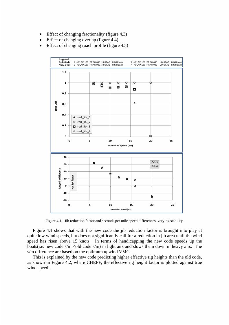
• Effect of changing fractionality (figure 4.3) • Effect of changing overlap (figure 4.4) • Effect of changing roach profile (figure 4.5)

LegendOLD Code _1 - O'LAP 150 FRAC 090 HI STAB IMS Roach _2 - O'LAP 150 FRAC 090_ LO STAB IMS RoachNEW Code _3 - O'LAP 150 FRAC 090 HI STAB IMS Roach _4 - O'LAP 150 FRAC 090_ LO STAB IMS Roach

RED

_JIB

0

0.2

0.4

0.6

0.8

1

1.2

0 5 10 15 20 25

True Wind Speed (kts)

red_jib _1

red_jib _2

red_jib _3

red_jib _4

‐20

‐10

0

10

20

30

40

0 5 10 15 20 25

Secs/m

ile differen

ce

True Wind Speed (kts)

1‐3

2‐4

+ve 3/4 faster

Figure 4.1 - Jib reduction factor and seconds per mile speed differences, varying stability.

Figure 4.1 shows that with the new code the jib reduction factor is brought into play at quite low wind speeds, but does not significantly call for a reduction in jib area until the wind speed has risen above 15 knots. In terms of handicapping the new code speeds up the boats(i.e. new code s/m <old code s/m) in light airs and slows them down in heavy airs. The s/m difference are based on the optimum upwind VMG.

This is explained by the new code predicting higher effective rig heights than the old code, as shown in Figure 4.2, where CHEFF, the effective rig height factor is plotted against true wind speed.

LegendOLD Code _1 - O'LAP 150 FRAC 090 Hi STAB IMS Roach _2 - O'LAP 150 FRAC 090_ Low STAB IMS RoachNEW Code _3 - O'LAP 150 FRAC 090 Hi STAB IMS Roach _4 - O'LAP 150 FRAC 090_ Low STAB IMS Roach

CH

EFF

0.9

0.95

1

1.05

1.1

1.15

1.2

1.25

1.3

1.35

1.4

0 5 10 15 20 25

True Wind Speed (kts)

cheff _1cheff _2cheff _3cheff _4

Figure 4.2 - Effective rig height factor vs. true wind speed.

Figure 4.3 shows the variation in Effective Rig height factor and the s/m differences for fractionalities of 0.85 and 1. The upper part of the figure shows that the effective height for the new code is greater for the mast head rig boat (Frac.=100%), and also the difference between CHEFF for the different fractionalities is much greater.

This gives rise to a speeding up of the mast head boats using the new code, which is most pronounced in light airs.

LegendOLD Code _1 - O'LAP 100 FRAC 085 Norm STAB IMS Roach _2 - O'LAP 100 FRAC 100. Norm STAB IMS RoachNEW Code _3 - O'LAP 100 FRAC 085 Norm STAB IMS Roach _4 - O'LAP 100 FRAC 100. Norm STAB IMS Roach

CH

EFF

0.9

0.95

1

1.05

1.1

1.15

1.2

1.25

1.3

1.35

1.4

0 5 10 15 20 25

True Wind Speed (kts)

cheff _1cheff _2cheff _3cheff _4

‐20

‐10

0

10

20

30

40

50

60

70

0 5 10 15 20 25

Secs/m

ile differen

ce

True Wind Speed (kts)

1‐3

2‐4

+ve 3/4 faster

Figure 4.3 – Effective rig height factor vs. True wind speed for 85% and 100% fractionality.

LegendOLD Code _1 - O'LAP 100 FRAC 090 Norm STAB IMS Roach _2 - O'LAP 135 FRAC 090. Norm STAB IMS RoachNEW Code _3 - O'LAP 100 FRAC 090 Norm STAB IMS Roach _4 - O'LAP 135 FRAC 090. Norm STAB IMS Roach

CH

EFF

0.9

0.95

1

1.05

1.1

1.15

1.2

1.25

1.3

1.35

1.4

0 5 10 15 20 25

True Wind Speed (kts)

cheff _1cheff _2cheff _3cheff _4

‐20

‐10

0

10

20

30

40

50

0 5 10 15 20 25

Secs/m

ile differen

ce

True Wind Speed (kts)

1‐3

2‐4

+ve 3/4 faster

Figure 4.4 - Effective rig height factor vs. true wind speed for different Overlap (100% & 135%).

Figure 4.4 shows the variation of effective rig height factor for different overlaps (100% & 135 %) at 90% fractionality. Here again the effective rig height is higher for the new code and the differences between overlaps are more pronounced for the new code. This results in the new code speeding up the boats in light airs, with the 135% ovelap yachts being sped up most.

LegendOLD Code _1 - O'LAP 100 FRAC 090 Norm STAB IMS Roach _2 - O'LAP 100 FRAC 090. Norm STAB HIR RoachNEW Code _3 - O'LAP 100 FRAC 090 Norm STAB IMS Roach _4 - O'LAP 100 FRAC 090. Norm STAB HIR Roach

CH

EFF

0.9

0.95

1

1.05

1.1

1.15

1.2

1.25

1.3

1.35

1.4

0 5 10 15 20 25

True Wind Speed (kts)

cheff _1cheff _2cheff _3cheff _4

‐20

‐10

0

10

20

30

40

50

0 5 10 15 20 25

Secs/m

ile differen

ce

True Wind Speed (kts)

1‐3

2‐4

+ve 3/4 faster

Figure 4.5 - Effective rig height factor vs. true wind speed for different Roach Profile

Figure 4.5 shows the effect of increasing mainsail roach. As expected the new code predicts higher effective rig heights for both the mainsails, and the high roach mainsail has a higher CHEFF than the IMS girth mainsail. This results in slightly higher predicted speeds for the high roach mainsail  

5 CONCLUSIONS This paper describes part of a more comprehensive general research program started in

2005 with partial funding from the ORC with the aim to investigate a series of rig planform variations in mainsail roach, jib overlap and rig fractionality in order to overcome some perceived inequities in the ratings of boats of various rig design racing under the International Measurement System (IMS).

Moreover activities carried out in order to address new sail configurations in the rating process and in particular Code0 have been described.

The results of this investigation are used to assist the International Technical Committee (ITC) in changing the formulations in the ORC INTERNATIONAL VPP sail aerodynamic model. In particular a new progressive de-powering approach has been included in the VPP code leading to a more realistic sail reduction process based on the application of a two stage reefing process (first a jib reduction from maximum to minimum area followed by a mainsail area reduction).

REFERENCES [1] Kerwin, J.E. A velocity Prediction Program for Ocean racing yachts, Rep 78-11 MIT,

July 1978

[2] Poor C.L., Sironi N., The International ,measurement system: a description of the new international rating system, 11th HISWA Symposium, Amsterdam, 1990

[3] Fossati F., Muggiasca S., Viola I. : An investigation of aerodynamic force modeling for IMS Rule using wind tunnel techniques – 19th HISWA Symposium, Amsterdam, 2006

[4] Campbell I.M.C.. Optimisation of a sailing yacht rig using wind tunnel data. The Thirteenth Chesapeake Sailing Yacht Symposium, Annapolis, 1997

[5] Edited by Claughton, Wellicome, & Shenoi, Sailing Yacht Design Theory Longman 1998 ISBN 0-582-36856-1

[6] Claughton, A, Developments in the IMS VPP Formulations, The 14th Chesapeake Sailing yacht symposium, Annapolis, USA, 1999

[7] Teeters J, Ranzenbach R, Prince M, Changes to Sail Aerodynamics in the IMS Rule. The 16th Chesapeake Sailing yacht symposium, Annapolis, USA, 2003