CHANDRA EXPOSURE ON SLOAN DIGITAL SKY SURVEY …

The Astrophysical Journal, 690:644–669, 2009 January 1 doi:10.1088/0004-637X/690/1/644c© 2009. The American Astronomical Society. All rights reserved. Printed in the U.S.A.

A FULL YEAR’S CHANDRA EXPOSURE ON SLOAN DIGITAL SKY SURVEY QUASARS FROM THECHANDRA MULTIWAVELENGTH PROJECT

Paul J. Green1,8

, T. L. Aldcroft1, G. T. Richards

2, W. A. Barkhouse

3,8, A. Constantin

1, D. Haggard

4, M. Karovska

1,

D.-W. Kim1, M. Kim

5, A. Vikhlinin

1, S. F. Anderson

4, A. Mossman

1, V. Kashyap

1, A. C. Myers

6, J. D. Silverman

7,

B. J. Wilkes1, and H. Tananbaum

11 Harvard-Smithsonian Center for Astrophysics, 60 Garden Street, Cambridge, MA 02138, USA; [email protected]

2 Department of Physics, Drexel University, 3141 Chestnut Street, Philadelphia, PA 15260, USA3 Department of Physics, University of North Dakota, Grand Forks, ND 58202, USA

4 Department of Astronomy, University of Washington, Seattle, WA, USA5 International Center for Astrophysics, Korea Astronomy and Space Science Institute, Daejeon, 305-348, Korea

6 Department of Astronomy, University of Illinois at Urbana-Champaign, Urbana, IL 61801, USA7 Institute for Astronomy, ETH Zurich, 8093 Zurich, Switzerland

Received 2008 May 15; accepted 2008 August 25; published 2008 December 1

ABSTRACT

We study the spectral energy distributions and evolution of a large sample of optically selected quasars from theSloan Digital Sky Survey that were observed in 323 Chandra images analyzed by the Chandra MultiwavelengthProject. Our highest-confidence matched sample includes 1135 X-ray detected quasars in the redshift range0.2 < z < 5.4, representing some 36 Msec of effective exposure. We provide catalogs of QSO properties,and describe our novel method of calculating X-ray flux upper limits and effective sky coverage. Spectroscopicredshifts are available for about 1/3 of the detected sample; elsewhere, redshifts are estimated photometrically.We detect 56 QSOs with redshift z > 3, substantially expanding the known sample. We find no evidence forevolution out to z ∼ 5 for either the X-ray photon index Γ or for the ratio of optical/UV to X-ray flux αox.About 10% of detected QSOs show best-fit intrinsic absorbing columns greater than 1022 cm−2, but the fractionmight reach ∼1/3 if most nondetections are absorbed. We confirm a significant correlation between αox andoptical luminosity, but it flattens or disappears for fainter (MB � −23) active galactic nucleus (AGN) alone.We report significant hardening of Γ both toward higher X-ray luminosity, and for relatively X-ray loud quasars.These trends may represent a relative increase in nonthermal X-ray emission, and our findings thereby strengthenanalogies between Galactic black hole binaries and AGN. For uniformly selected subsamples of narrow-lineSeyfert 1s and narrow absorption line QSOs, we find no evidence for unusual distributions of either αox or Γ.

Key words: galaxies: active – quasars: absorption lines – quasars: general – surveys – X-rays: general

Online-only material: color figures, machine-readable tables

1. INTRODUCTION

Interest in the properties of active galaxies and their evolu-tion has recently intensified because of deep connections be-ing revealed between supermassive black holes (SMBHs) andgalaxy evolution, such as the relationship between the massof galaxy spheroids and the SMBHs they host (the MBH–σconnection; Ferrarese & Merritt 2000; Gebhardt et al. 2000).A feedback paradigm could account for this correlation,whereby winds from active galactic nuclei (AGNs) moderatethe SMBH growth by truncating that of their host galaxies (e.g.,Granato et al. 2004). Feedback models may explain the corre-spondence between the local mass density of SMBHs and theluminosity density produced by high-redshift quasars (Yu &Tremaine 2002; Hopkins et al. 2006) as well as the “cosmicdownsizing” (decrease in the space density of luminous AGNs)seen in AGN luminosity functions (Barger et al. 2005; Hasinger2005; Scannapieco et al. 2005). If quasar activity is inducedby massive mergers (e.g., Wyithe & Loeb 2002, 2005), thenthe jigsaw puzzle now assembling may merge smoothly withcosmological models of hierarchical structure formation.

8 Visiting Astronomer, Kitt Peak National Observatory, Cerro TololoInter-American Observatory, and National Optical Astronomy Observatory,which is operated by the Association of Universities for Research inAstronomy, Inc. (AURA), under cooperative agreement with the NationalScience Foundation.

Many, if not most, of the accreting SMBHs in the universemay be obscured by gas and dust in the circumnuclear region, orin the extended host galaxy. The obscured fraction may dependon both luminosity and redshift (Ueda et al. 2003; Brandt &Hasinger 2005; La Franca et al. 2005), and is indeed likely toevolve on grounds both theoretical (e.g., Hopkins et al. 2006a)and observational (Treister & Urry 2006; Ballantyne et al. 2006).Such evolution seems to be required for AGN populations tocompose the observed spectrum of the cosmic X-ray background(CXRB; Gilli et al. 2007). However, a full census of all SMBHsremains observationally challenging, since some are heavilyobscured, or accreting at very low rates, below the sensitivitylimits of current telescopes even at low redshifts.

AGN unification models explain many of the observed dif-ferences in the spectral energy distributions (SEDs) of AGNsas being due to the line-of-sight effects of anisotropic distribu-tions of obscuring material near the SMBH (Antonucci 1993).The intrinsic number ratio of obscured-to-unobscured AGN mayevolve, and is almost certainly a function of luminosity. Indeed,the ratio in the Seyfert (low-) luminosity regime is currentlyestimated to be ∼4, whereas for the QSO (high-) luminosityregime, it may be closer to unity (Gilli et al. 2007).

Astronomers, like most people, usually look where they cansee. Type 1 quasars are the easiest AGNs to find in largenumbers via either spectroscopic or color selection becauseof their broad emission lines (FWHM � 1000 km s−1) and

644

http://dx.doi.org/10.1088/0004-637X/690/1/644

mailto:[email protected]

No. 1, 2009 PROPERTIES OF SDSS QUASARS IN THE ChaMP 645

generally blue continuum slopes and brighter magnitudes. Mostof these show few other signs of obscuration such as infraredexcess or weakened X-ray emission. Large samples of Type 1QSOs—as the brightest high-redshift objects—have servedto probe intervening galaxies, clusters, and the intergalacticmaterial (IGM) along the line of sight, right to the epoch ofre-ionization. Because observed SEDs are thought to be lessaffected by obscuration and therefore more representative ofintrinsic accretion physics, the evolution of this Type 1 sampleis of interest as well.

The SEDs and clustering properties of Type 1 QSOs have beenstudied in increasing detail, probing farther into the universe andwider across the sky and the electromagnetic spectrum. SEDsincluding mid-infrared photometry from Spitzer were compiledand characterized recently for 259 quasars from the SloanDigital Sky Survey (SDSS) by Richards et al. (2006b). Thesestudies are most useful for calculating bolometric luminositiesand K-corrections toward understanding the energetics of theaccretion process, and its evolution across cosmic time. Studiesthat target SDSS QSO pairs with small separations find asignificant clustering excess on small scales (� 40 kpc h) ofvarying strengths (e.g., Hennawi et al. 2006; Myers et al. 2007,2008), which could be due to mutual triggering, or might simplyresult from the locally overdense environments in which quasarsform (Hopkins et al. 2008).

Optical luminosity function studies of optically selectedquasars (e.g., Richards et al. 2006a, 2005; Croom et al. 2004)date back decades (e.g., Boyle et al. 1988). Accurate luminosityfunctions are needed to trace the accretion history of SMBHsand to contrast the buildup of SMBHs with the growth of galaxyspheroids. An increasing number of optical surveys not onlyselect AGNs photometrically, but also determine fairly reliablephotometric redshifts for them. These samples stand to vastlyimprove the available statistical reliability and the resolutionavailable in the luminosity/redshift plane.

X-ray observations have been found to efficiently selectAGNs of many varieties, and at higher surface densities thanever (Hasinger 2005). Independent of the classical AGN opticalemission line criteria, X-rays are a primary signature of accre-tion onto a massive compact object, and the observed X-raybandpass corresponds at higher redshifts to rest-frame ener-gies capable of penetrating larger intrinsic columns of gas anddust.9 Even for Type 1 QSOs, X-ray observations have revealednew connections (e.g., between black holes from 10 to 109M�;Maccarone et al. 2003; Falcke et al. 2004) and new physical in-sights such as the possibility of ubiquitous powerful relativisticoutflows (Middleton et al. 2007) or of relativistically broad-ened fluorescent Fe Kα emission (see, e.g., the review articlesby Fabian et al. 2000; Reynolds & Nowak 2003). Quasars withbroad absorption lines (BAL QSOs) blueward of their UV emis-sion lines turn out to be highly absorbed in X-rays (Green et al.1995, 2001; Green 1996; Gallagher et al. 2002). Quasars thatare radio loud are 2–3 times brighter in X-rays for the sameoptical magnitude (Zamorani et al. 1981; Worrall et al. 1987;Shen et al. 2006), and also may have harder X-ray spectra (e.g.,Shastri et al. 1993, although see Galbiati et al. 2005).

The high sensitivity and spatial resolution of Chandra andXMM-Newton open other avenues for exploration of quasars andtheir environments. Clusters of galaxies have been discoveredin the vicinity of, or along the sightlines to quasars (Green

9 The observed-frame, effective absorbing column is NeffH ∼ NH/(1 + z)2.6

(Wilman & Fabian 1999).

et al. 2005; Siemiginowska et al. 2005). Lensed quasars havenow been spatially resolved in X-rays, unexpectedly showingsignificantly different flux ratios than at other wavebands (Greenet al. 2002; Blackburne et al. 2006; Lamer et al. 2006).

The expected evolution in the environment, accretion rates,and masses of SMBHs in AGNs should correspond to observ-able evolution in their SEDs. The two most common X-raymeasurements used are the X-ray power-law photon index Γ10

and the X-ray-to-optical spectral slope, αox.11 Many of the ap-parent correlations have been challenged as being artifacts ofselection or the by-products of small, heterogeneous samples,which impede progress in our understanding of quasar physicsand evolution.

The archives of current X-ray imaging observatories such asChandra and XMM-Newton are growing rapidly, and severallarge efforts for pipeline processing, source characterization(Ptak & Griffiths 2003; Aldcroft 2006), and catalog generationare underway. The 2XMM catalog (006) is available,and the Chandra source catalog12 is due out in 2008 (Fabbianoet al. 2007).

Serendipitous wide-area surveys with Chandra were pi-oneered by the Chandra Multiwavelength Project (ChaMP;Green et al. 2004; Kim et al. 2004) for high Galactic lati-tude, while ChaMPlane (Grindlay et al. 2005) has studied thestellar content of Galactic plane fields. The ChaMP, describedin more detail below, also performs multiwavelength sourcematching and spectroscopic characterization. These efforts aregreatly augmented by large surveys such as the SDSS (Yorket al. 2000), which will obtain spectroscopy of ∼100,000 QSOs(e.g., Schneider et al. 2007), and can additionally facilitate theefficient extrapolation of photometric quasar selection with pho-tometric redshift estimation almost a magnitude fainter, towarda million QSOs (e.g., Richards et al. 2008).

The current paper studies the X-ray and optical properties ofthe subset of these QSOs imaged in X-rays by Chandra as partof the ChaMP (Green et al. 2004).

2. THE QUASAR SAMPLE

2.1. The SDSS Quasar Sample

Most large samples of Type 1 QSOs are based on opticallyselected quasars confirmed via optical spectroscopy (Boyleet al. 1988; Schneider et al. 1994; Hewett et al. 1995). Thelargest, most uniform sample of optically selected quasars byfar has been compiled from the SDSS. With the completionof the SDSS, we can expect some 100,000 spectroscopicallyconfirmed quasars. The SDSS quasars were originally identifiedto i < 19.1 for spectroscopy by their UV-excess colors, withlater expansion for z > 3 quasars to i = 20.2 using ugri colorcriteria (Richards et al. 2002). The large catalog, the broad-wavelength optical photometry, and subsequent follow-up inother wavebands have meant that research results from the SDSSspectroscopic quasar sample better characterize the breadth ofthe quasar phenomenon than ever before. However, the limitednumber of fibers available, fiber placement conflicts, and aboveall the bright magnitude limits of SDSS fiber spectroscopy mean

10 Γ is the photon number index of an assumed power-law continuum suchthat NE(E) = NE0 EΓ. In terms of a spectral index α from fν = fν0 ν

α , wedefine Γ = (1 − α).11 αox is the slope of a hypothetical power law from 2500 Å to 2 keV;αox = 0.3838 log(l2500Å/l2 keV).12 The Chandra source catalog Web page is http://cxc.harvard.edu/csc.

http://cxc.harvard.edu/csc

646 GREEN ET AL. Vol. 690

that 10 times as many quasars have been imaged, and could beefficiently identified from existing SDSS photometry.

Using large spectroscopic AGN samples as “training sets”can produce photometric classification and redshifts of fargreater completeness and depth than spectroscopy. Withoutspectroscopic confirmation, photometric selection criteria strikea quantifiable balance between completeness and efficiency, i.e.,a probability can be assigned both to the classification and theredshift. Deep photometric redshift surveys like COMBO-17(Wolf et al. 2003) have found AGNs to R = 24 and z = 5 withhigh completeness. Efficient photometric selection of quasars inthe SDSS using a nonparametric Bayesian classification basedon kernel density estimation is described in Richards et al.(2004) for SDSS point sources with i < 21. An empiricalalgorithm to determine photometric redshifts for such quasars isdescribed in Weinstein et al. (2004). The spectroscopic trainingsamples for these methods now include far more high-redshiftquasars, and so the algorithms have been retrained to includeobjects redder than (u − g) = 1.0 to classify high-z quasars,and applied to the much larger SDSS Data Release 6 (DR6).This large catalog of ∼1 million photometrically identifiedQSOs and their photometric redshifts is described in Richardset al. (2008). They estimate the overall efficiency of the catalogto be better than 72%, with subsamples (e.g., X-ray detectedobjects) being as efficient as 97%. These estimates are basedon an analysis of the autoclustering of the objects in the catalog(Myers et al. 2006), which is very sensitive to stellar interlopers.However, at the faint limit of the catalog some additional galaxycontamination is expected.

For luminosity and distance calculations, we adopt an H0 =70 km s−1 Mpc−1, ΩΛ = 0.7, and ΩM = 0.3 cosmologythroughout. We assume α = −0.5 for the optical continuumpower-law slope (v ∝ να , where ν is the emission frequency),and derive the rest-frame, monochromatic optical luminosity at2500 Å (l2500Å; units erg s−1Hz−1) using the SDSS dereddenedmagnitude with central wavelength closest to (1 + z) × 2500 Å.

2.2. The Extended Chandra Multiwavelength Project

The ChaMP is a wide-area serendipitous X-ray survey basedon archival X-ray images of the (|b| > 20 deg) sky observedwith the AXAF CCD Imaging Spectrometer (ACIS) onboardChandra. The full 130-field Cycle 1–2 X-ray catalog is public(Kim et al. 2007b), and the most comprehensive X-ray numbercounts (log N–log S) to date have been produced thanks to 6600sources and massive source-retrieval simulations (Kim et al.2007a). We have also published early results of our deep (r ∼25) NOAO/MOSAIC optical imaging campaign (Green et al.2004), now extended to 67 fields (W. A. Barkhouse et al. 2009,in preparation). ChaMP results and data can be found online.13

To improve statistics and encompass a wider range of sourcetypes, we have recently expanded our X-ray analysis to covera total of 392 fields through Chandra Cycle 6. We choseonly fields overlapping with SDSS DR5 imaging. To easeanalysis and minimize bookkeeping problems, the new list ofChandra pointings (observation IDs; “obsids” hereafter) avoidsany overlapping observations by eliminating the observationwith the shorter exposure time. As described in Green et al.(2004), we also avoid fields with large (� 3′) extended sources ineither optical or X-rays (e.g., nearby galaxies M101, NGC 4725,NGC 4457, or clusters of galaxies MKW8, or Abell 1240).Spurious X-ray sources (due to, e.g., hot pixel, bad bias, bright

13 http://hea-www.harvard.edu/CHAMP

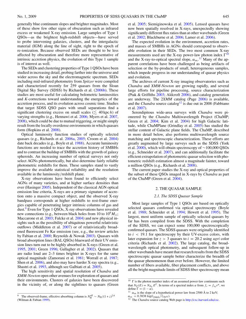
Figure 1. Sky area vs. B-band (0.5–8 keV) flux limit for the 323 obsids includedin our ChaMP/SDSS field sample. Flux limit is defined here as the number ofcounts detectable in 90% of simulation trials, converted to flux assuming apower-law Γ = 1.7 at z = 0 and the Galactic NH appropriate to each obsid.Chip S4 (CCD ID 8) is excluded throughout. The area covered at the brightestfluxes is 32 deg2.

source readout streaks) have been flagged and removed asdescribed in Kim et al. (2007b). Of the 392 ChaMP obsids,323 overlap the SDSS DR5 footprint.

The ChaMP has also developed and implemented anxskycover pipeline which creates sensitivity maps for allChaMP sky regions imaged by ACIS. This allows (1) iden-tification of imaged-but-undetected objects, (2) counts limitsfor 50% and 90% detection completeness, and (3) correspond-ing flux upper limits at any sky position, as well as (4) fluxsensitivity versus sky coverage for any subset of obsids, asneeded for log N–log S and luminosity function calculations.Our method is described in the Appendix, and has been verifiedrecently by Aldcroft et al. (2008) using the Chandra Deep FieldSouth (CDF-S). The final sky ChaMP/SDSS coverage area (indeg2) for the 323 overlapping fields as a function of broadband(B band 0.5–8 keV) flux limit is shown in Figure 1 (see cap-tion for specific definition of this limit). The area covered at thebrightest fluxes is 32 deg.2 On average five CCDs are activatedper obsid.

We have downloaded into the ChaMP database all the SDSSphotometry, and the list of photo-z quasar candidates within 20′of the Chandra aim point for each such obsid.14 Because theChandra point-spread function (PSF) increases with off-axisangle (OAA), comparatively few sources are detected beyondthis radius, and source centroids also tend to be highly uncertain.Of X-ray detected candidates, we will show in Section 2.4 that98% of these candidates with spectra are indeed QSOs.

Next we describe the identification of high-confidenceChaMP X-ray counterparts to SDSS QSOs in Section 2.3. Wethen discuss in Section 2.4 spectroscopic identifications for theseobjects. Section 3 then describes results for several interestingQSO subsamples, including our treatment of SDSS quasars thatwere not X-ray detected.

14 For 14 obsids, we extended to 28′ radius, to achieve full coverage of theChandra footprint. For other obsids, the SDSS imaging strips do notcompletely cover the Chandra field of view.

http://hea-www.harvard.edu/CHAMP


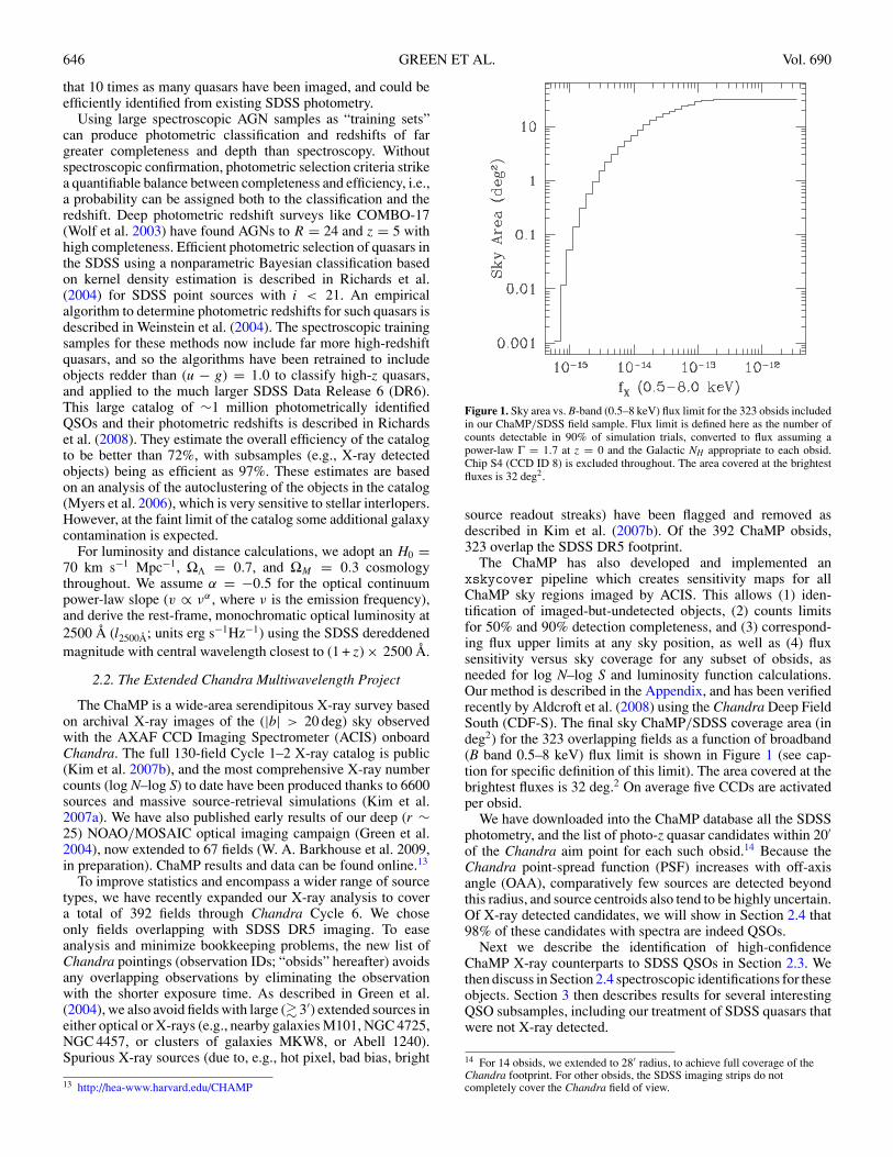
Figure 2. Positional offsets of matched sample. Left: the histogram of X-ray/optical centroid separations in the full matched sample of 1376. The mode is 0.′′3, themedian is 0.′′76, and the mean is 1.′′1. Right: the ratio of the X-ray/optical centroid separation to the 95% X-ray positional uncertainty vs. separation. The fraction ofobjects with separations larger than the 95% uncertainty (i.e., with ratio greater than 1) remains relatively constant, and virtually no separations wider than 3′′ arelarger than the positional uncertainty σXP95.

2.3. X-Ray/Optical Matching

The positional uncertainty of ChaMP X-ray source centroidshas been carefully analyzed via X-ray simulations by Kimet al. (2007a) and depends strongly on both the number ofsource counts and the OAA. Cross-correlating ChaMP X-raysource centroids with QSOs, we find that 95% of the X-ray/optical separations dXO of matched QSOs are smaller thanthe 95% X-ray positional uncertainty σXP95. We first performan automated matching procedure between each optical QSOposition and the ChaMP’s X-ray source catalog. We adopt 4′′as our matching radius criterion. Figure 2 shows that 95% ofthe matched sample has an X-ray/optical position differenceof less than 3′′, and expansion to include match radii above 4′′would not substantially increase the sample size. Searching theChaMP catalog for X-ray sources within 4′′ of the optical SDSSquasar coordinate, yields 1376 unique matches in the “Matched”sample.

Although the overall efficiency of the SDSS photometric QSOcatalog is only expected to be 72% (Richards et al. 2008), therarity of luminous Type 1 quasars and X-ray sources means thatmatched objects should be quite clean. By repeatedly offsettingthe SDSS coordinates of each QSO by 36′′ and rematchingto the ChaMP X-ray catalog, we derive a spurious matchrate of just 0.7%.15 This excellent result is due to Chandra’s∼ arcsec spatial resolution, which at SDSS depths allows forunambiguous counterpart identification, given that both Type 1QSOs and X-ray sources are relatively sparse on the sky.

We identify and remove a variety of objects with potentiallypoor data, including overlapping multiple sources (some ofwhich are targeted lenses), bright X-ray sources suffering frompile-up, optical sources with photometry contaminated by closebrighter sources or within large extended galaxies, or stellardiffraction spikes.

In addition to the automated matching procedure, we alsoperform visual inspection (VI) of both X-ray and optical

15 The ratio of the number of X-ray matches to the optical control sample tothe number of matches in the actual sample is 0.0067.

images, overplotting the centroids and their associated po-sition errors. We retain only the highest-confidence matches(matchconf=3). Most of the 105 objects we thereby eliminatehave large ratios of dXO/σXP95, or multiple candidate opticalcounterparts. We note that some of the most interesting celes-tial systems may be found among sources with matchconf<3.For example, these might include QSOs that are lensed, havebright jets, or are associated with host or foreground opticalclusters or galaxies. Systems that are poorly matched, multiplymatched, or photometrically contaminated may account for upto ∼10% of the full X-ray-selected sample. We therefore cautionagainst blind cross-correlation of large source catalogs (e.g., theChandra Source Catalog)16 without such detailed quality con-trol and visual examination of images. However, since we seekhere to analyze the multiwavelength properties of a large cleansample of QSOs, and since most of these more complicatedsystems require significant further analysis or observation, wedefer their consideration to future studies.

2.4. Spectroscopic Redshift Information

After cross-correlation with the X-ray catalog, we soughtspectroscopic redshifts for any objects in the photometric QSOcatalog. For this purpose, we obtained redshifts from existingChaMP spectroscopy, from the SDSS (DR6) database itself,and then finally we searched the literature by cross-correlatingoptical positions with the NASA Extragalactic Database (NED),using a 2′′ match radius. Of 1376 matched objects, we found highconfidence spectroscopic redshifts for 407, of which 43 spectrawere observed by the ChaMP. In striking testimony to the qualityof the quasar selection algorithm (especially once candidateshave been matched to X-ray sources) only eight of these (2%) arenot broad-line AGNs. Three are narrow emission line galaxies,two are absorption line galaxies (no emission lines of equivalentwidth Wλ > 5 Å), and three are known BL Lac objects. Weexclude these objects from all samples described below. Because

16 The Chandra Source Catalog, available at http://cxc.cfa.harvard.edu/csc,contains all X-ray sources detected by the Chandra X-ray Observatory.

http://cxc.cfa.harvard.edu/csc


Figure 3. SDSS i magnitude vs. broadband (0.5–8 keV) X-ray flux for theSDSS/ChaMP QSO the Main sample. The flux shown is based on the best-fit PL-free yaxx model, with the effect of Galactic absorption removed fromboth X-ray and optical. X-ray detections are marked by black dots and fluxupper limits by green arrows. The open red triangles show QSOs with existingspectroscopic redshifts, clearly biased toward brighter optical mags. Radio-loud quasars (large open blue circles), BAL QSOs (open black squares), NALQSOs (open black diamonds) and NLS1s (open black triangles), and ChandraPI targets (large asterisks) are also indicated as shown in the legend.

(A color version of this figure is available in the online journal.)

the magnitude distribution (and therefore the photometric colorerrors) for objects lacking spectroscopic classifications is fainter(see Figure 3), we expect that the overall fraction of misclassifiedphoto-z QSOs is larger than 2%, but it would be difficult toestimate it without deeper spectroscopic samples. A plot of thephotometric versus spectroscopic redshifts of these quasars isshown in Figure 4.

3. SAMPLES, SUBSAMPLES, AND DETECTIONFRACTIONS

The definition of our Main sample and a variety of subsamplesare described in subsequent sections and summarized in Table 1.The size of our Main sample allows us to investigate the effectsof luminosity or redshift limits, X-ray nondetections, PI targetbias, strong radio-related emission (RL QSOs), broad- andnarrow-line absorption (BAL and NAL, respectively, QSOs),and Narrow-Line Seyfert 1s (NLS1s). In Table 1, samples towhich we refer frequently are arrayed under “Primary Samples”in decreasing order of the number of detections. Samplesmentioned only once or twice in this paper are listed in similarorder under “Other Samples.” Tables listing bivariate statisticalresults (Tables 5–7) later in the paper list samples in this sameorder for reference.

We define the Main sample to be the 2308 SDSS QSOs thatfall on Chandra ACIS chips in a region of effective exposuregreater than 1200 s (excluding CCD 8; see below), regardless ofChandra X-ray detection status. Our cleaned matched sample(the MainDet sample) of X-ray/optical matched QSOs contains1135 distinct X-ray sources with high optical counterpart matchconfidence, where we have removed all sources (1) with signif-icant contamination by nearby bright optical sources, (2) withsignificant overlap with other X-ray sources, (3) with detected

on ACIS-S chip S4 (CCD 8), because of its high backgroundand streaking, (4) with dithering across chips (which rendersunreliable the yaxx X-ray spectral fitting described below), or(5) with spectroscopy indicating that the object is not a Type 1QSO.

The mean exposure time for the MainDet sample is25.9 ks per QSO, with an average of 3.6 QSOs detected oneach Chandra field.17 For the 1173 nondetections in the Mainsample, the mean exposure time is 17.6 ks. A histogram ofexposure times for all QSOs in the Main sample is shown inFigure 5.

We publish key data for 1135 QSOs in the MainDet samplein Table 2, marking 82 sources that are the intended Chandraprincipal investigator (PI) targets. X-ray sources in plots includeonly the MainDet sample or subsets of it. Figure 6 showsluminosity versus redshift for the MainDet sample. A largefraction of the z > 4 objects are Chandra targets (large blackstars). Strong redshift–luminosity trends are seen both in opticaland X-ray, as is expected from any flux-limited survey. However,the factor ∼30–50 range in luminosity is unusual for a singlesample; such breadth is usually only achieved using samplecompilations encompassing diverse selection techniques. InFigure 6, the large number of objects in our sample makes itdifficult to distinguish the point-types presenting object classinformation, so Figure 7 shows a zoom-in on the most denselypopulated regions of the L–z plane.

Since we start with Type 1 SDSS QSOs, we are studying anoptically selected sample, and the selection function is complex(Richards et al. 2006a). If we limit the analysis to detectionsonly, then the sample is both optically and X-ray selected, andthe selection function becomes increasingly complex. If insteadwe include all X-ray upper limits in the analysis, the sampleremains fundamentally optically selected, but then statisticalanalyses must incorporate the nondetections (see Section 6.1).

The ChaMP’s xskycover pipeline allows us to investigatethe detection fraction for the full SDSS QSO sample, shownin Figure 8. Of 2308 SDSS QSOs that fall on an ACIS chip(the Main sample) in our 323 ChaMP fields, 1135 (49%)are detected in the MainDet sample. Detection fractions as afunction of SDSS QSO mag and redshift for this sample areshown in Figure 9. To minimize sample biases, we can alsoexamine detection fractions as a function of X-ray observingparameters like exposure time and OAA. To simultaneouslyoptimize detected sample size and detection fraction, we simplymaximize N2

det

/Nlim, where Ndet and Nlim are the number

of X-ray detections and nondetections (flux upper limits),respectively. We find that an X-ray-unbiased subsample witha significantly higher detection rate is achieved by limitingconsideration to the 1269 QSOs with OAA < 12′ and exposuretime T > 4 ks, of which 922 (72%) are detections. This highdetection fraction sample is called the D2L sample (Table 1).

Data for X-ray nondetections is available in Table 3. We in-clude in Table 3 only the 347 limits in the D2L sample, wherethe flux limits are sensitive enough to be interesting. By “inter-esting,” we mean that the limits are close to or brighter thanthe faint envelope of detections. A flux limit several timesbrighter than that envelope provides no statistical constraintswhatsoever on the derived distributions or regressions. For X-raynondetections, data are more sparse all around for several rea-sons. QSOs with limits are optically fainter (mean and mediani = 20.4 mag for the D2L sample limits compared to i = 19.9

17 For 14 of 323 Chandra fields, no QSOs are detected.


Figure 4. Left: photometric redshift vs. spectroscopic redshift for QSOs detected in ChaMP fields. Filled (red) circles show QSOs for which the formal photometricredshift probability is greater than 95%. A fraction of objects have large errors in their photometric redshifts. About 18% of QSOs with zspec < 1 have zphot > 2.This drops to 13% using only Prob(zphot) > 0.5. Right: difference between the photometric and true (spectroscopic) redshift for QSOs in our sample, plotted againstphotometric redshift probability, again illustrates the reliability of these probabilities.


Figure 5. Left: histogram of effective Chandra exposure times for QSOs in the Main sample, in units of ks, with bin size 6 ks for detections (solid black line) and limits(dashed blue line). For detections, the mean and median exposure times are 25.9 and 17.6 ks, respectively. The inset shows detail at low exposure times using bin size1 ks. Right: histogram of Chandra OAAs for the Main sample, in units of arcmin. The black solid histogram shows how detections trend toward small OAA. Meanand median for detections are 6.′4 and 5.′8, respectively. Blue histogram shows that limits trend toward large OAA. The dashed histograms show the correspondingcumulative fractions. About 90% of the detections (compared to ∼ 50% of the limits) are at OAA < 12′ off-axis.


for detections). Being fainter, fewer have SDSS spectroscopy.Also, as nondetections, none have been targeted for spectraby the ChaMP, so globally only about 10% of nondetectedQSOs have optical spectra. The fraction of radio detections isalso smaller (1.2% versus 4.8%). None are Chandra PI targets.Finally, X-ray nondetections lacking optical spectroscopy aresomewhat less likely to be QSOs. The selection efficiency (frac-tion of QSO candidates that are actual QSOs) between about0.8 < z < 2.4 is ∼95% (Richards et al. 2004; Myers et al.2006), but Richards et al. (2008) estimate that near the faint

limit of i ∼ 20.4 mag, the overall QSO selection efficiencyis ∼80%. Particular attention must be paid to possible galaxycontamination at the faint end as the autoclustering estimatesof the efficiency do not include galaxy interlopers at faint lim-its where SDSS star–galaxy separation begins to break down.However, many of these “spurious” cross-matches may turn outto be (e.g., low-luminosity) AGNs. In any case, the increasedlevel of contamination by non-QSOs is another rationale forlimiting the number of nondetections to those with sensitiveX-ray limits. The nature of the statistical analysis (as discussed


Table 1Quasar Sample Definitions

Sample Limsa Targets RL Absb Tmin OAA Ndet Nlim Ntotal % Det

Primary SamplesMain y . . . . . . . . . . . . . . . 1135 1173 2308 49MainDet . . . . . . . . . . . . . . . . . . 1135 0 1135 100noTDet . . . n . . . . . . . . . . . . 1053 0 1053 100D2L y . . . . . . . . . 4 12 922 347 1269 72D2LNoRB y . . . n n 4 12 866 338 1204 71hiLo y . . . n n . . . . . . 847 961 1808 46HiCtNoTRB . . . n n . . . . . . . . . 129 0 129 100

Other SamplesNoRB y . . . n n . . . . . . 1054 1144 2198 47NoRBDet . . . . . . n n . . . . . . 1054 0 1054 100D2LNoTRB y n n n 4 12 828 338 1166 71hiLoLx . . . . . . n n . . . . . . 801 0 801 100zLxBox . . . . . . . . . . . . . . . . . . 817 0 817 100LoBox . . . . . . . . . . . . . . . . . . 530 0 530 100zBox y . . . . . . . . . . . . . . . 420 360 780 53zBoxDet . . . . . . . . . . . . . . . . . . 420 0 420 100D2LSy1 y . . . n n . . . . . . 176 84 260 68HiCt . . . . . . . . . . . . . . . . . . 157 0 157 100HiCtNoTRB . . . n n n . . . . . . 129 0 129 100

Notes.a If “y,” sample includes X-ray nondetections.b If “n,” sample excludes QSOs with evident BALs or NALs and also NLS1s.

in Section 6.1) is such that nondetections are included, but areassumed to follow the distribution of detections, and so effec-tively have a lower weight in the results.

Amongst the undetected QSOs in the Main sample, 165have SDSS spectroscopy, of which 144 are high confidencespectroscopic QSOs. The 21 non-QSOs comprise 16 stars andfive galaxies. The higher (13%) rate of nonstar spectroscopicclassifications amongst undetected QSOs is not surprising, sinceX-ray detection greatly increases the probability that an opticalAGN candidate is indeed an AGN. From the upper limit QSOsample, we remove the 22 non-QSOs, and use the SDSSspectroscopic redshifts instead of the photometric redshiftswherever applicable.

3.1. Targets

The “Nontarget” detected sample (the noTDet sample) of1053 QSOs further eliminates 82 objects (7.2% of the MainDetsample) that are the intended targets of the Chandra observa-tion wherein they are found. Targets are on average brighterthan most of the QSO sample (see Figure 3), but more im-portantly were chosen for observation for a variety of reasonsunrelated to this study. In particular, targets tend to be moreluminous than serendipitous QSOs (Figures 6 and 7), and sev-eral are known lenses (e.g., HS 0818+1227, PG 1115+080,UM 425 = QSO 1120+019). The bias in sample characteris-tics is largely mitigated in the subsamples excluding targets (seeTable 1). However, the exclusion of targets also produces a(much smaller) bias because some objects with similar charac-teristics would have been included (at a lower rate) were theChandra pointings all truly random. Because many of the tar-gets are indeed of interest (e.g., high-z QSOs), we include themin most discussions, but always check that results are consis-tent without them. We also note that some target bias probablyaffects the X-ray sample even after the exclusion of PI targetQSOs, because PI targets may cluster with other categories ofX-ray sources such as other AGN, galaxies, or clusters. Overall,

a comparison of regression results18 for several of our subsam-ples that differ only in target exclusion does not indicate a sig-nificant target bias, due at least in part to our large sample sizes.

3.2. Radio Loudness

Quasars with strong radio emission are observed to be moreX-ray luminous (e.g., Green et al. 1995; Shen et al. 2006).At least some of the additional X-ray luminosity is likely tooriginate in physical processes related to the radio jet ratherthan to the accretion disk, so it may be important to recognizethose objects that are particularly radio loud.

The Faint Images of the Radio Sky at Twenty Centimeters(FIRST) survey (Becker et al. 1995) from the NRAO Very LargeArray (VLA) has a typical (5σ ) sensitivity of ∼1 mJy, and coversmost of the SDSS footprint on the sky. Following Ivezic et al.(2002), we adopt a positional matching radius of 1.′′5, whichshould result in about 85% completeness for core-dominatedsources, with a contamination of ∼3%. We thereby match 69sources to the Matched sample. Jiang et al. (2007) matched theFIRST to SDSS spectroscopic quasars and found that about 6%matched within 5′′. We might expect a lower matched fractionbecause our optical photometric sample extends 1–2 mag fainter.On the other hand, we are looking at X-ray-detected quasars, sothe actual matched fraction of ∼5% is similar. We also matchedall the quasar optical positions to the FIRST within 30′′, andvisually examined all the FIRST images to look for multiplematches and/or lobe-dominated quasars. There are 26 sourcesthat we judged to have reliable morphological complexity thatare resolved by FIRST into multiple sources. The NRAO VLASky Survey (NVSS; Condon et al. 1998), lists detections for19 of these. Comparing NVSS with summed FIRST fluxes, wefound NVSS fluxes slightly larger: less 2% difference in themean (∼20% max). Since the NVSS beam is larger (45′′) than

18 Table 6 and 7 shows similar results comparing, e.g., the MainDet sampleand the noTDet sample, or the D2LNoRB sample and the D2LNoTRB sample.

No.1,2009

PRO

PER

TIE

SO

FSD

SSQ

UA

SAR

SIN

TH

EC

haMP

651

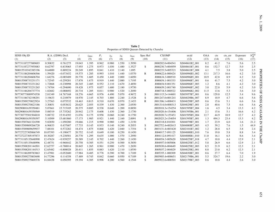
Table 2Properties of SDSS Quasars Detected by Chandra

SDSS Obj ID R.A. (J2000) Decl. i zphot Pz zlo zhi zbest Spec Ref CXOMP srcid OAA cts cts_err Exposure NGalH

(1) (2) (3) (4) (5) (6) (7) (8) (9) (10) (11) (12) (13) (14) (15) (16) (17)

587731187277889693 0.50832 0.761275 19.043 1.395 0.962 0.980 1.550 1.3950 J000202.0+004541 XS04861B2_001 8.2 41.2 7.6 5.6 2.5587731187277955083 0.62797 0.833065 17.955 1.275 0.973 1.030 1.480 1.3527 S J000230.7+004959 XS04861B7_001 0.6 132.7 12.7 5.0 2.5588015510343385196 0.64800 0.889224 20.249 1.895 0.841 1.410 2.140 1.895 J000235.5+005321 XS04861B7_008 4.1 7.5 3.8 5.0 2.5587731186204606566 1.59420 −0.073452 19.575 1.285 0.993 1.010 1.440 1.0370 R J000622.6-000424 XS04096B5_002 13.1 217.3 16.6 4.2 3.0587731186204606704 1.64276 −0.085489 20.770 1.605 0.450 1.440 2.000 1.6050 J000634.3-000510 XS04096B5_001 10.9 42.8 8.9 4.2 3.0588015508733231171 1.72545 −0.259281 17.878 1.675 0.919 1.440 2.080 1.7195 R J000654.1-001533 XS04096B7_001 0.6 41.7 7.5 4.2 3.0588015508733231262 1.72868 −0.230998 20.345 2.485 0.552 2.110 2.670 2.4850 J000654.9-001351 XS04096B7_003 1.2 8.6 4.1 4.2 3.0588015508733231265 1.74704 −0.294690 19.428 1.975 0.857 1.600 2.180 1.9750 J000659.2-001740 XS04096B7_002 3.0 22.8 5.9 4.2 3.0587731186204737774 1.82682 −0.088692 20.734 1.205 0.811 0.900 1.520 1.2050 J000718.5-000522 XS04096B2_002 11.5 13.6 5.3 3.6 3.0587730773889974538 2.81349 14.767168 18.276 4.665 0.976 4.490 5.070 4.9672 S J001115.2+144601 XS03957B7_001 0.6 129.8 12.5 3.4 9.6587731186742198291 3.19633 0.210979 18.970 2.145 0.703 1.880 2.240 2.1528 S J001247.0+001241 XS04829B6_007 8.9 10.9 4.7 6.6 5.6588015509270822924 3.27563 0.075532 18.463 0.815 0.510 0.670 0.970 2.1453 R J001306.1+000431 XS04829B7_005 0.6 15.6 5.1 6.6 5.6588015509270823186 3.30851 0.053632 20.625 2.055 0.539 1.430 2.300 2.0550 J001314.0+000313 XS04829B7_001 2.8 40.6 7.5 6.6 5.6588290881639350481 5.07661 15.715105 20.375 0.885 0.538 0.640 1.200 0.8850 J002018.3+154254 XS01595B7_004 1.6 4.5 3.4 13.3 4.2588290881639350569 5.08519 15.735262 20.942 2.175 0.608 1.430 2.360 2.1750 J002020.4+154406 XS01595B6_001 2.1 15.6 5.1 16.6 4.2587730775501504810 5.08732 15.914392 21.076 0.175 0.958 0.060 0.240 0.1750 J002020.7+155451 XS01595B5_004 12.7 44.9 10.9 12.7 4.2588290881639350397 5.10509 15.681860 17.173 1.985 0.921 1.440 2.160 2.0091 S J002025.2+154054 XS01595B7_001 1.3 494.3 23.4 13.3 4.2588015507661324390 5.82850 −1.050280 19.666 1.215 0.990 0.980 1.450 1.2150 J002318.8-010301 XS04079B7_001 1.7 23.9 6.0 1.6 21.2588015509809266720 6.96833 0.437687 17.733 0.145 0.933 0.140 0.240 0.2053 S J002752.4+002615 XS04080B7_003 4.5 39.2 7.6 1.5 44.9588015509809659937 7.88101 0.572282 18.474 1.875 0.868 1.620 2.040 1.7354 S J003131.4+003420 XS02101B7_002 1.2 28.8 6.5 3.8 2.4587727227305066749 10.07393 −9.190477 20.752 0.145 0.649 0.100 0.250 0.1450 J004017.7-091125 XS04888B3_010 7.6 19.8 5.8 8.8 3.4587727227305197873 10.30287 −9.238581 20.770 1.295 0.635 1.000 1.570 1.2950 J004112.6-091417 XS04888B1_010 11.0 16.1 6.5 8.6 3.4587731185135648990 12.47624 −0.939257 20.389 2.145 0.702 1.440 2.260 2.1450 J004954.3-005620 XS04825B7_018 4.7 10.8 4.4 12.9 2.1587731185135648996 12.48751 −0.968442 20.758 0.385 0.551 0.250 0.500 0.3850 J004957.0-005806 XS04825B7_012 5.8 26.9 6.6 12.9 2.1588015508201144501 12.62757 −0.780014 20.845 1.265 0.961 0.900 1.470 1.2650 J005030.6-004649 XS04825B2_003 8.5 21.9 6.2 12.3 2.1588015508201144513 12.65482 −0.808028 20.411 1.855 0.883 1.620 2.110 1.8550 J005037.2-004829 XS04825B2_001 8.8 23.8 6.2 12.3 2.1587731186209783863 13.47981 −0.052600 17.984 0.485 0.778 0.390 0.700 1.7189 S J005355.1-000309 XS04830B7_001 0.6 27.7 6.4 7.0 1.9588015509275803698 14.77296 0.114358 17.489 0.745 0.842 0.660 0.950 0.7189 S J005905.4+000651 XS02179B6_001 5.5 324.7 19.6 2.2 3.0588015509275869378 14.84438 0.050395 19.194 4.385 0.998 4.200 4.560 4.1544 S J005922.6+000301 XS02179B7_003 0.6 10.8 4.4 2.6 3.0

652G

RE

EN

ET

AL

.V

ol.690

Table 2(Continued.)

SDSS Obj ID NintrH Nhi

H N loH Γ Γhi Γlo log fx log l2 keV log l2500 Å αox f20 cm Ext R Class Targ Comments

(1) (18) (19) (20) (21) (22) (23) (24) (25) (26) (27) (28) (29) (20) (31) (32) (33)

587731187277889693 1.53 0.45 −0.44 −12.960 26.988 30.590 1.383 0 1.06 0 0587731187277955083 2.40 0.42 −0.38 −12.850 27.065 30.978 1.502 0 0.62 0 1588015510343385196 2.14 1.25 −1.03 −13.990 26.286 30.391 1.576 0 1.54 0 0587731186204606566 0.00 0.27 0.00 1.74 0.30 −0.24 −12.321 27.308 30.020 1.041 3897.60 1 4.86 0 0 NED: FBQS J0006-0004587731186204606704 1.31 0.49 −0.46 −12.870 27.228 29.899 1.025 0 1.75 0 0588015508733231171 2.05 0.46 −0.44 −13.180 26.992 31.173 1.605 0 0.59 0 1 NED: LBQS 0004-0032588015508733231262 3.50 1.87 −1.26 −14.000 26.563 30.650 1.569 0 1.58 0 0588015508733231265 2.27 0.68 −0.62 −13.470 26.850 30.758 1.500 0 1.21 0 0587731186204737774 1.82 0.91 −0.79 −13.230 26.561 29.765 1.230 0 1.73 0 0587730773889974538 1.88 0.37 −0.35 −12.580 28.701 32.063 1.290 0 0.75 0 1587731186742198291 2.13 1.02 −0.89 −13.730 26.681 31.020 1.666 0 1.03 0 0588015509270822924 2.10 0.87 −0.74 −13.820 26.587 31.220 1.778 0 0.82 1 1 HiBAL NED: LBQS 0010-0012588015509270823186 1.47 0.43 −0.41 −13.220 27.142 30.316 1.218 0 1.69 0 0588290881639350481 2.05 1.48 −1.24 −14.640 24.819 29.639 1.850 0 1.59 0 0588290881639350569 1.72 0.73 −0.67 −14.010 26.412 30.241 1.470 0 1.82 0 0587730775501504810 1.69 0.70 −0.63 −13.450 24.354 27.578 1.238 0 1.87 0 0588290881639350397 0.00 0.47 0.00 1.77 0.16 −0.12 −12.609 27.729 31.676 1.515 0 0.31 0 1588015507661324390 1.94 0.60 −0.57 −13.000 26.799 30.231 1.317 0 1.31 0 0588015509809266720 1.28 0.50 −0.46 −12.540 25.418 29.033 1.388 0 0.53 3 1 NLSy1588015509809659937 2.23 0.58 −0.54 −13.360 26.822 30.939 1.581 0 0.83 0 0587727227305066749 1.91 0.73 −0.67 −13.540 24.084 27.718 1.395 0 1.74 0 0587727227305197873 1.16 0.79 −0.73 −13.410 26.458 29.783 1.276 0 1.75 0 0587731185135648990 0.95 0.89 −0.86 −13.950 26.457 30.449 1.532 0 1.60 0 0587731185135648996 2.30 0.65 −0.59 −13.810 24.775 28.568 1.456 0 1.74 0 0588015508201144501 2.79 0.90 −0.80 −13.690 26.153 29.830 1.412 0 1.78 0 0588015508201144513 1.77 0.71 −0.62 −13.580 26.673 30.307 1.395 0 1.60 0 0587731186209783863 0.90 0.48 −0.48 −13.300 26.871 31.118 1.630 0 0.63 2 1 Many strong NALs588015509275803698 0.00 0.47 0.00 1.61 0.26 −0.16 −11.751 27.486 30.690 1.230 2508.80 1 3.84 0 0588015509275869378 1.32 0.84 −0.77 −13.410 27.688 31.542 1.480 0 1.12 0 1

Notes. (1) SDSS Object ID, (2) SDSS R.A. (J2000), (3) SDSS decl. (J2000), (4) SDSS asinh mag_psf i, dereddened, (5) photometric redshift (see, Weinstein et al. 2004), (6) photometric redshift range probability,(7) lower limit of photometric redshift range, (8) upper limit of photometric redshift range, (9) best redshift: spectroscopic if different than zphot, (10) reference for spectroscopic redshift—S: SDSS, O: ChaMP, R:published reference from NED, (11) ChaMP IAU source name, (12) ChaMP internal source ID, format XSoooooBc_nnn where ooooo is Chandra obsid, c is ACIS CCD ID, and nnn is source ID on that CCD, (13)Chandra OAA in arcmin, (14) net 0.3–8 keV source counts, (15) rms uncertainty on net counts, (16) vignetting-corrected exposure time in ks, (17) galactic column in units 1020 cm−2, (18) best-fit X-ray intrinsic columnin 1022 cm−2, only included four counts > 200, (19) 90% upper limit on intrinsic column in 1022 cm−2, (20) 90% lower limit on intrinsic column in 1022 cm−2, (21) best-fit X-ray power-law index Γ, (22) 90% upperlimit on Γ, (23) 90% lower limit on Γ, (24) log X-ray flux (0.5–8 keV) in erg cm−2 s−1, (25) log X-ray luminosity at 2 keV in erg s−1 Hz−1, (26) log optical/UV luminosity at 2500 Å in erg s−1 Hz−1, (27) αox, theoptical/UV to X-ray spectral index, (28) 20 cm radio flux in mJy from FIRST or NVSS, (29) radio extent flag, (30) radio loudness R, (31) spectral class: 1, BAL; 2, NAL; 3, NLS1, (32) 1, intended Chandra PI target,(33) comments.(This table is available in its entirety in a machine-readable form in the online journal. A portion is shown here for guidance regarding its form and content.)


Figure 6. Luminosity at 2500 Å (left) and 2 keV (right) vs. redshift for the SDSS/ChaMP in the Main sample. Above z ∼ 2.5, the number of QSOs declines steeply,due to the SDSS magnitude limit and due to the decreased efficiency of the photometric selection algorithm as it crosses the stellar color locus (see Figure 8 andRichards et al. 2002). These plots show 56 QSOs with z > 3, of which 34 are new serendipitous detections. X-ray upper limits are shown as small green triangles here.See Figure 3 for symbol types. The dashed black rectangle surrounds the zBoxDet sample, a portion of the l2500 Å−z plane chosen to test for redshift dependence. Thegreen rectangle “LoptBox” surrounds the LoBox sample, used to test for dependence on l2500 Å. The blue rectangle surrounds the zLxBox sample, chosen to avoidX-ray flux limit bias.


Figure 7. Left: zoom-in of 2500 Å luminosity vs. redshift. Objects with spectroscopic redshifts (open red triangles) tend to be at high optical luminosities by selection.Detectably radio-loud QSOs are shown with open blue circles. See Figure 3 for symbol types. BAL QSOs (open black squares) are mostly detected at z > 1.6 wherethe CIV region enters the optical bandpass. There appears to be no preference of BAL QSOs for high optical luminosity, apart from the bias caused by Chandra targetselection. Right: zoom-in of 2 keV luminosity vs. redshift. Here, the RL QSOs clearly populate the upper luminosity envelope. BAL QSOs are preferentially X-rayquiet, unlike the QSOs with NALs only (open diamonds).


FIRST (5′′), FIRST detection algorithms may exclude some ofthe extended source flux as background, so we include the NVSSfluxes for these 19 objects, and summed FIRST fluxes for thoseremaining.

Following Ivezic et al. (2002), we adopt a radio-loudnessparameter R as the logarithm of the ratio of the radio tooptical monochromatic flux: R = log(F20 cm/Fi) = 0.4(i −m20 cm), where m20 cm is the radio AB magnitude (Oke & Gunn1983), m20 cm = −2.5 log(F20 cm/3631 Jy) calculated from theintegrated radio flux density, and i is the SDSS i-band magnitude,corrected for Galactic extinction. We adopt a radio-loudnessthreshold R = 1.6. Thus there are 72 QSOs in the Main samplewith radio detections, of which 57 (79%) are radio loud. For theMainDet sample (detections only), there are 55 radio-detectedQSOs, of which 43 (78%) are radio-loud. Figure 10 shows radioloudness versus redshift for the MainDet sample. Many of theradio upper limits are near our adopted radio loudness threshold.

Given the (∼ 1 mJy) source detection limit of the FIRSTSurvey, all RL QSOs will be detected to about i ∼ 20.4 mag. Forthe magnitude range 17 < i < 20 where the statistics are goodand the FIRST is sensitive to all RL QSOs, we find 41 of 529(8 ± 1%) such QSOs from the MainDet sample are detected bythe FIRST, with 29 (5.4%) that are radio loud. Since the 34% ofour full the MainDet sample that is fainter than i = 20.4 suffersfrom incomplete radio-loudness measurements, some 2% maybe unidentified RL QSOs. A similar fraction pertains if we countX-ray nondetections as well (the Main sample).

3.3. Broad and Narrow Absorption Line Quasars

We identified QSOs with BALs and NALs directly by visualinspection of QSOs with spectroscopy, finding 16 BAL and11 NAL QSOs in the MainDet sample. Ten (two) of the BAL(NAL) QSOs were the Chandra PI targets.


Figure 8. Left: histogram of redshifts for detected (solid blue), nondetected (red dashed), and all (black solid) QSOs in the MainDet sample. We tally the “best”redshift for each object (i.e., spectroscopic redshifts are always used when available). Above z ∼ 2.5, the number of QSOs declines steeply, due to the decreasedefficiency of the photometric selection algorithm as it crosses the stellar color locus (Richards et al. 2002). The inset shows the detected fraction as a function ofredshift. Right: histogram of SDSS i mag for detected (solid blue), nondetected (red dashed), and all (black solid) QSOs. The inset shows the detected fraction as afunction of magnitude.


Figure 9. Left: histogram of redshifts for detected (solid blue), nondetected (red dashed), and all (black solid) QSOs, after restriction to obsids with T > 4 ks andQSOs with OAA less than 12′ (the D2L sample). The inset shows the detected fraction as a function of redshift. Right: histogram of SDSS i mag for detected (solidblue), nondetected (red dashed), and all (black solid) QSOs. The inset shows the detected fraction as a function of magnitude.


The best estimates to date of the raw BAL QSO fractionamong optically selected quasars range from about 13–20%(Reichard et al. 2003; Hewett & Foltz 2003). From the SDSSDR3 sample of Trump et al. (2006), Knigge et al. (2008)carefully define what is a BAL QSO and correct for a varietyof selection effects to derive an estimate of the intrinsic BALQSO fraction of 17% ± 3. The vast majority of BAL QSOsin the SDSS are above redshift 1.6 because only then doesthe CIV absorption enter the spectroscopic bandpass.19 If wedetermine our BAL QSO fraction in the MainDet sampleby only counting the serendipitous (nontarget) QSOs with

19 A much smaller number of the rare low-ionization BAL QSOs (with BALsjust blueward of Mg ii) are found at lower redshifts.

z > 1.6 and spectroscopic redshifts, we find just 4 out of119 QSOs with BALs. Even with sensitive X-ray observationssuch as these, X-ray selection is strongly biased against thehighly ionized absorbing columns along the line of sighttoward the X-ray emitting regions of BAL QSOs. Of the24 absorbed (BAL or NAL) QSOs, two are detectably radioloud; SDSS J171419.24+611944.5—a BAL QSO—and SDSSJ171535.96+632336.0—a NAL QSO—are targets selected (byChandra PI Richards) as reddened QSOs.

3.4. Narrow-Line Seyfert 1s

X-rays from NLS1s are of particular interest because theywere thought to show marked variability and strong soft


Figure 10. Radio-loudness vs. redshift for the MainDet sample (detections).Radio-loud objects R > 1.6 are shown with open blue circles. Radio-quietbut FIRST radio-detected objects are shown as filled green circles. All othersymbols (described in Figure 3) have radio flux upper limits only. Note thatmost Chandra targets are distinctly either loud or quiet, highlighting a bias inthe target subsamples.


X-ray excesses (e.g., Green et al. 1993; Boller et al. 1996).NLS1s are proposed to be at one extreme of the so-called(Boroson & Green 1992) “eigenvector 1,” which has beensuggested to correspond to low SMBH masses (Grupe et al.2004) and/or high (near-Eddington) accretion rates (Boroson2002).

For objects with SDSS spectra encompassing Hβ (z < 0.9),we identify as NLS1s (Osterbrock & Pogge 1985) those objectswith FWHM(Hβ) < 2000 km s−1and line flux ratio [O iii]/Hβ <3. The FWHM measurements are obtained via FWHM =2.35 c σ/λ0/(1 + z), where σ 2 is the variance of the Gaussiancurve that fits the Hβ emission line, z is the redshift, and λ0 isthe rest-frame wavelength of the Hβ line (4863 Å). We extractmeasurements of σ (in Å) and line fluxes from the SDSS DR6SpecLine table.

Our MainDet sample contains at least 19 NLS1s (thosewith spectroscopy in the redshift range to include Hβ).Among the nondetections, we identify three more. Six of these22 objects are targets described in Williams et al. (2004),and SDSS J125140.33+000210.8 was a target selected (byChandra PI Richards) as a dust-reddened QSO. The Williamset al. (2004) sample consisted of 17 SDSS NLS1s selected fromthe ROSAT All Sky Survey to be X-ray weak. Their study con-firmed earlier suggestions that strong, ultrasoft X-ray emissionis not a universal characteristic of NLS1s.

We therefore present here new results for a sample of 15SDSS NLS1s observed by Chandra. This admittedly smallsample is nevertheless the largest published sample of opticallyselected NLS1s with unbiased X-ray observations. The sampleof Williams et al. (2004) was selected to be X-ray weak, whilethe Grupe et al. (2004) ROSAT sample was selected to havestrong soft X-ray emission. We find no evidence for unusualSEDs from the distributions of either αox or Γ.

4. OPTICAL COLORS AND REDDENING

In Figure 11, we plot the (g − i) colors of the matchedSDSS/ChaMP QSO sample as a function of redshift, andcompare to the optical-only sample.20 The Chandra-detectedsample does not show significantly different colors from the fulloptical sample. This likely attests to (1) the sensitivity of theChandra imaging relative to the magnitude limit of the opticalsample and (2) the fact that Type 1 QSOs are largely unabsorbedin both the optical and X-ray regimes.

The right panel of Figure 11 shows that 10 of 14 BAL QSOsare above the Δ (g − i) = 0 line. This reflects that SDSS BALQSOs tend to be redder than average (Reichard et al. 2003; Daiet al. 2007). Most of the RL QSOs are also redder than average.Richards et al. (2001) found a higher fraction of intrinsicallyreddened quasars among those with FIRST detections. Ivezicet al. (2002) found that RL QSOs are redder than the mean(at any given redshift) in (g − i) by 0.09 ± 0.02 mag.Figure 11 confirms a similar trend in the X-ray detected SDSS/ChaMP sample. At the same time, a small number of RL QSOsare found on the blue extreme of the color-excess distribution.These trends are fully consistent with the detailed results foundby stacking FIRST images of SDSS quasars (White et al. 2007),independent of X-ray properties.

5. X-RAY SPECTRAL FITTING WITH yaxx

Besides comparing the broadband multiwavelength proper-ties of QSOs, Chandra imaging provides X-ray spectral resolu-tion capable of yielding significant constraints on the propertiesof emission arising nearest the SMBH. While the ChaMP cal-culates hardness ratios (HRs) and appropriate errors for everysource, these can be difficult to interpret, since HR convolvesthe intrinsic quasar SED with telescope and instrument responseand does not take redshift or Galactic column NGal

H into account.A direct spectral fit of the counts distribution using the full in-strument calibration, known redshift, and NGal

H provides a muchmore direct measurement of quasar properties. Note that evenin the low-count regime, one can obtain robust estimates of fitparameter uncertainties using the Cash (1979) fit statistic.

We use an automated procedure to extract the spectrum andfit up to three models to the data. For all objects in the Matchedsample, we first define a circular source region centered onthe X-ray source which contains 95% of 1.5 keV photons atthe given OAA. An annular background region is also centeredon the source with a width of 20′′. We exclude any nearbysources from both the source and background regions. We thenuse CIAO21 tool psextract to create a PHA (pulse heightamplitude) spectrum covering the energy range 0.4–8 keV.

Spectral fitting is done using the CIAO Sherpa22 tool inan automated script known as yaxx23 (Aldcroft 2006). Allof the spectral models contain an appropriate Galactic neutralabsorber. For all sources we first fit two power-law models whichinclude a Galactic absorption component frozen at the 21 cmvalue24: (1) fitting photon index Γ, with no intrinsic absorption

20 The optical-only sample refers to all SDSS QSOs within ∼20′ of allChandra pointings, regardless of whether its position falls on an ACIS CCD.We use a 9th-order polynomial fit to the optical-only sample with thefollowing coefficients: 0.698892, 3.011733, −20.358267, 37.850353,−33.617121, 16.652032, −4.861889, 0.833027, −0.077526, and 0.003026.21 http://cxc.harvard.edu/ciao22 http://cxc.harvard.edu/sherpa23 http://cxc.harvard.edu/contrib/yaxx24 Neutral Galactic column density NGal

H taken from Dickey & Lockman(1990) for the Chandra aim-point position on the sky.

http://cxc.harvard.edu/ciao

http://cxc.harvard.edu/sherpa

http://cxc.harvard.edu/contrib/yaxx

656G

RE

EN

ET

AL

.V

ol.690

Table 3Properties of SDSS Quasars with Chandra Limits

SDSS Obj ID R.A. (J2000) Decl. i zphot Pz zlo zhi zbest Spec Ref obsid ccdid OAA counts < Exposure NGalH log fx < log l2 keV < log l2500 Å αox > f20cm R Class Notes

(1) (2) (3) (4) (5) (6) (7) (8) (9) (10) (11) (12) (13) (14) (15) (16) (17) (18) (19) (20) (21) (22) (23) (24)588015510343385295 0.56337 0.909429 20.956 4.6050 0.949 4.440 5.22 4.6050 4861 7 6.4 16.0 4.5 2.5 −13.650 27.554 30.856 1.268 1.82 0588015510343385302 0.63485 0.870704 20.819 2.2250 0.415 1.840 2.70 2.2250 4861 7 2.8 10.0 4.6 2.5 −13.865 26.581 30.311 1.432 1.77 0588015509270823376 3.32406 0.057045 20.984 0.0650 0.616 0.060 0.12 0.0650 4829 7 3.5 11.1 6.0 5.6 −13.926 22.955 26.290 1.280 1.83 0588015509270888717 3.40998 0.141416 20.457 1.4450 0.615 0.960 1.61 1.4450 4829 3 9.0 20.2 4.4 5.6 −13.239 26.747 30.023 1.258 1.62 0588015509270888725 3.45158 0.098009 20.804 1.4950 0.774 0.950 2.22 1.4950 4829 3 10.8 22.7 4.6 5.6 −13.211 26.811 29.915 1.191 1.76 0587730775501504550 5.00208 15.852781 19.190 1.6850 0.915 1.440 2.11 1.7510 S 1595 5 10.7 25.3 5.3 4.2 −13.405 26.786 30.742 1.519 1.12 0587727180601295054 10.04659 −9.111831 20.220 2.0950 0.653 1.290 2.26 2.0950 4888 3 7.5 17.2 7.8 3.4 −13.668 26.714 30.495 1.452 1.53 0587727180601557048 10.60443 −8.983756 19.739 1.8750 0.916 1.590 2.13 1.8750 4886 2 9.9 22.6 6.9 3.6 −13.498 26.766 30.586 1.466 1.34 0587727227305394556 10.73418 −9.141124 20.920 0.1450 0.370 0.140 0.25 0.1450 4886 1 2.3 9.4 7.9 3.6 −13.930 23.694 27.029 1.280 1.81 0587727180601622916 10.82587 −9.032790 20.550 2.8550 0.866 2.520 3.26 2.8550 4886 0 8.1 17.7 7.0 3.6 −13.605 27.104 30.574 1.332 1.66 0587731185135649019 12.55619 −0.978559 20.734 0.3950 0.575 0.240 0.98 0.3950 4825 7 6.2 15.1 11.4 2.1 −14.075 24.536 28.869 1.663 1.73 0588015508201144424 12.68671 −0.838214 20.077 0.5850 0.525 0.420 0.68 0.5850 4825 3 10.0 22.7 5.9 2.1 −13.317 25.702 29.374 1.410 1.47 0588015509275279576 13.48778 0.041851 21.014 2.3550 0.485 2.080 2.73 2.3550 4830 6 5.1 12.8 5.0 1.9 −13.635 26.871 30.327 1.327 1.85 0587731186209849918 13.50874 −0.132789 20.138 4.6750 0.958 4.480 4.87 4.6750 4830 7 5.7 14.0 6.2 1.9 −13.843 27.376 31.176 1.459 1.49 0587731511532454189 19.71203 −0.963115 20.433 2.3950 0.849 2.190 2.92 2.3950 4963 7 4.1 15.0 36.9 14.1 −14.575 25.949 30.534 1.760 1.61 0587731511532454208 19.75317 −0.964191 20.711 0.1250 0.503 0.120 0.25 0.1250 4963 7 4.2 14.8 36.5 14.1 −14.577 22.908 27.428 1.735 1.72 0588015507667419343 19.83900 −1.181540 19.716 1.4350 0.927 1.140 1.53 1.4350 4963 5 11.1 43.3 20.3 14.1 −13.737 26.241 30.318 1.565 1.33 0587727884161581293 29.96522 −8.803312 20.815 0.1250 0.597 0.120 0.26 0.1250 6106 3 3.2 12.0 32.7 15.9 −14.453 23.032 27.465 1.702 1.77 0587727883893211318 30.05424 −8.839227 20.380 1.8250 0.479 1.440 2.01 1.8250 6106 2 5.0 13.9 29.1 15.9 −14.342 25.893 30.304 1.693 1.59 0587727178999398623 30.28336 −9.408542 20.874 2.4850 0.686 2.060 2.76 2.4850 3772 7 3.5 11.4 13.2 24.2 −14.278 26.284 30.470 1.607 1.79 0587731512611897674 32.80721 −0.133716 20.592 1.4450 0.561 0.960 1.66 1.4450 2081 7 3.2 10.2 4.0 2.7 −13.872 26.113 29.957 1.475 1.68 0587731513691013244 45.00239 0.807781 16.531 4.3850 0.990 4.190 4.51 4.3850 4145 7 0.6 7.7 4.0 7.0 −13.875 27.278 32.749 2.100 0.05 0587731512083349864 51.75811 −0.573625 20.969 1.1150 0.702 0.620 1.66 1.1150 5810 2 8.4 18.3 7.8 6.7 −13.624 26.083 29.515 1.317 1.83 0587728906098377011 115.26597 31.160109 18.733 3.8450 0.971 3.370 4.35 3.8450 0377 7 3.4 11.7 26.1 4.2 −14.530 26.488 31.669 1.989 0.93 0587728906098376844 115.31801 31.184168 20.169 4.8350 0.983 4.510 5.52 4.8350 0377 7 1.8 9.8 25.5 4.2 −14.595 26.658 31.268 1.770 1.51 0588007005767532860 116.33380 39.501996 20.363 0.8250 0.582 0.390 1.01 0.8250 6111 1 5.6 14.5 28.7 8.3 −14.298 25.086 29.585 1.727 1.59 0588007005767532880 116.44541 39.466243 20.179 2.0250 0.738 1.820 2.19 2.0250 6111 1 10.7 34.7 35.6 8.3 −14.014 26.333 30.480 1.592 1.51 0587731680110052241 116.73920 27.665360 20.778 4.6050 0.984 4.440 5.19 4.6050 3561 7 3.2 10.4 4.4 4.7 −13.833 27.371 31.001 1.394 1.75 0587725470127095818 118.81215 41.058484 19.824 1.6150 0.725 1.440 1.95 1.6150 3032 2 11.5 25.7 4.1 8.5 −13.144 26.960 30.331 1.294 1.37 0

Notes. (1) SDSS object ID, (2) SDSS R.A. (J2000), (3) SDSS decl. (J2000), (4) SDSS asinh mag_psf i, dereddened, (5) photometric redshift (see Weinstein et al. 2004), (6) photometric redshift range probability, (7) lower limit of photometric redshiftrange, (8) upper limit of photometric redshift range, (9) best redshift: spectroscopic if different than zphot, (10) reference for spectroscopic redshift—S: SDSS, O: ChaMP, R: published reference from NED, (11) Chandra observation ID (obsid), (12)ACIS CCD id, (13) Chandra OAA in arcmin, (14) 99% counts upper limit the 0.3–8 keV range, (15) vignetting-corrected exposure time in ks, (16) galactic column in units 1020cm−2, (17) log upper limit to the X-ray flux (0.5–8 keV) in erg cm−2 s−1,(18) log upper limit to the X-ray luminosity at 2 keV in erg s−1 Hz−1, (19) log optical/UV luminosity at 2500 Å in erg s−1 Hz−1, (20) αox, the optical/UV to X-ray spectral index, (21) 20 cm radio flux in mJy from FIRST, (22) radio loudness, (23)class: 1, BAL; 2, NAL; 3, NLS1, (24) comments.

(This table is available in its entirety in a machine-readable form in the online journal. A portion is shown here for guidance regarding its form and content.)


Figure 11. Left: SDSS (g − i) color vs. best redshift. Symbols show individual QSOs in the SDSS/ChaMP the MainDet sample. The black line shows the mean colorat each redshift (in redshift bins of 0.12 for z < 2.5 and 0.25 for higher redshifts) for the full optical QSO sample (regardless of Chandra imaging). We derive a smooth(9th-order) polynomial fit to those means, whose value is plotted as the “expected” (g − i) with a green asterisk (at the redshift of each actual QSO). Right: the colorexcess Δ(g − i) (the difference between the actual and “expected” (g − i) color) is plotted against redshift for a limited redshift range, to show highlights. The residualsof the polynomial fit to the mean binned (g − i) of the full optical sample are shown connected by a solid green line. See Figure 3 for symbol types. Most targets, BALQSOs, and RL QSOs are redder than average.


component (model “PL”) and (2) fitting an intrinsic absorberwith neutral column N intr

H at the source redshift, with photonindex frozen at Γ = 1.9 (model “PLfix”). Allowed fit rangesare −1.5 < Γ < 3.5 for PL and 1018 < N intr

H < 1025 forPLfix. These fits use the Powell optimization method, andprovide a robust and reliable one-parameter characterizationof the spectral shape for any number of counts. Spectra withless than 100 net counts25 were fit using the ungrouped datawith Cash statistics (Cash 1979). Spectra with more than 100counts were grouped to a minimum of 16 counts per bin andfit using the χ2 statistic with variance computed from thedata.

Finally, X-ray spectra with over 200 counts were also fit witha two-parameter absorbed power law where both Γ and the NGal

H

were free to vary within the above ranges (model “PL_abs”).

5.1. X-Ray Spectral Continuum Measurements

We compile “best-PL” measurements, where for fewer than200 counts, we use Γ from the PL (N intr

H fixed at zero) fits andfor higher count sources we use PL_abs (both Γ and N intr

H free).In the MainDet sample there are 156 sources with 200 counts ormore. High-count objects are found scattered at all luminositiesbelow z ∼ 2.5. QSOs with more than 200 counts (0.5–8 keV)with both Γ and N intr

H fits in yaxx, are well-distributed in l2 keVamongst the detections due to the wide range of exposure times.

The mean Γ for all the 1135 QSOs in the MainDet sampleis 1.94 ± 0.02 with median 1.93. Means and medians for theMainDet sample and the subsamples discussed in this sectionare listed in Table 4. The typical (median) error in Γ, ΔΓ ∼ 0.5,is similar to the dispersion 0.54 in best-fit values of Γ. If welimit the sample to the 314 sources with more than 100 counts,

25 Source counts derived from yaxx may differ at the ∼1% level from thosederived by ChaMP XPIPE photometry, due to slightly different backgroundregion conventions.

the typical error is 0.32, with no change in mean or median Γ.The Γ distribution that we find is similar to that found recentlyfor smaller samples of broad-line AGNs (BLAGNs). Just et al.(2007) studied a sample of luminous optically selected quasarsobserved by Chandra, ROSAT, and XMM-Newton, and found〈Γ〉 = 1.92 ± 0.09 for 42 QSOs. Mainieri et al. (2007) studieda sample of 58 X-ray-selected BLAGNs in the XMM-COSMOSfields, and found 〈Γ〉 = 2.09 with a dispersion of ∼0.26. Page(2006) found 〈Γ〉 = 2.0 ± 0.1 with a dispersion of ∼0.36 for50 X-ray-selected BLAGN in the 13H XMM-Newton/Chandradeep field.

Figure 12 shows a histogram of best-fit power-law slopes forseveral interesting subsamples of QSOs from both the MainDetsample and from the noTDet sample which omits PI targets.The mean and median values for these subsamples are listed inTable 4. We do not separately plot the radio-quiet (RQ) QSOsample, since it follows quite closely the shape of the full samplehistogram.

For 43 detected RL QSOs in the MainDet sample, the nominalmean slope is 〈Γ〉 = 1.73 ± 0.05 with median 1.65, with adistribution significantly flatter than for the 704 definitively RQQSOs (〈Γ〉 = 1.91±0.02) in the MainDet sample, using the two-sample tests described in Section 6.1.1. RL QSOs are knownto have flatter high energy continua from previous work (e.g.,Reeves & Turner 2000).

For the 15 known BAL QSOs in the MainDet sample, thenominal mean slope is 〈Γ〉 = 1.35 ± 0.15 with median 1.3,and the distribution is significantly different than for the fullMainDet sample (minus BALs, NALs, and NLS1), using thetwo-sample tests described in Section 6.1.1. The difference iseven more significant (Pmax < 0.01%) when comparing onlyto the 667 definitively RQ QSOs (RL < 1.6). Since the mean(median) number of (0.5–8 keV) counts for BAL QSOs is just 27(15), the nominally lower Γ likely reflects undetected absorption(Green et al. 2001; Gallagher et al. 2002).


Figure 12. Left: histogram of best-fit X-ray spectral power-law slope Γ (best-PL) for the MainDet sample. The full sample (black solid) histogram has been dividedby 15, and the RL QSO (long-dashed black) histogram by 2, for ease of comparison with smaller subsamples. BAL QSOs (blue down-slash shading) show very flatslopes, due to strong intrinsic absorption. The NAL distribution (green up-slash shading) suggests a possible bimodality. Neither the NAL nor the NLS1 (magentadense shading) nor the high redshift (short-dashed red) histograms are significantly different, by the Kolmogorov–Smirnov (K-S) test from the full sample distribution.Right: the same plot, but for the noTDet sample which omits PI targets. The RL QSO distribution is less distinct here, and the softest (largest Γ) NLS1s disappear.


Table 4Quasar Sample Univariate Results

Samplea N Mean Errorb Median Pmaxc(%)

Γ Distributionsd

MainDet 1135 1.94 0.02 1.93 . . .

RQ 704 1.91 0.02 1.86 0.2RL 43 1.73 0.05 1.65 0.2BAL 15 1.35 0.15 1.30 0.05NAL 9 1.68 0.13 1.75 19NLS1 19 2.01 0.15 1.95 35z > 3 56 1.80 0.07 1.76 21

αox DistributionsD2L 1269 1.421 0.005 1.365 . . .

RQ 680 1.527 0.008 1.452 0.0RL 31 1.382 0.030 1.392 0.0BAL 23 1.717 0.028 1.664 0.0NAL 8 1.463 0.056 1.500 49NLS1 19 1.540 0.080 1.433 24z > 3 47 1.817 0.077 1.786 55

Notes.a For each parameter tested, the numeric sample at the top is the parent forcomparison subsamples below. The RL subsamples are tested against non-RLQSOs from the parent sample. The remaining three QSO subsamples for eachparameter are tested against the parent sample excluding all four QSO subtypes.b Error in the mean from the Kaplan–Meier estimator as implemented in ASURV.An estimate of the dispersion can be obtained by multiplying this by

√N − 1.

c The maximum probability for the null hypothesis (of indistinguishablesamples) from three tests described in Section 6.1.1. Only for Pmax < 5 dowe consider the distributions significantly different. RL and RQ samples arecontrasted to each other. Other samples are compared to their parent sample(MainDet or D2L) −X, where X = BALs + NALs + NLS1s, except for BALs,whose parent sample is RQ QSOs only.d These are distributions of “best-PL” measurements, best-fit Γ, which alwaysincludes NGal

H , and also includes NintrH for 0.5–8 keV counts > 200.

The mean slope 〈Γ〉 = 1.68 ± 0.13 with median 1.75 for thenine known NALs in the MainDet sample is indistinguishablefrom the full MainDet sample (minus BALs, NALs, and NLS1),but the NAL statistics are poor. On the other hand, a smaller, non-overlapping sample of NALs observed by Chandra publishedby Misawa et al. (2008) agrees that the X-ray properties of

intrinsic NAL quasars are indistinguishable from those of thelarger quasar population.

For the 19 known NLS1s in the MainDet sample, thenominal mean slope is 〈Γ〉 = 2.01 ± 0.15 with median 1.95,indistinguishable from the comparison sample (MainDet sampleminus BALs, NALs, and NLS1).

5.1.1. X-Ray Spectral Evolution

No signs of evolution have been detected for the intrinsicpower-law slope Γ of QSOs: z > 4 samples (Vignali et al. 2005;Shemmer et al. 2006) show Γ ∼ 2, just like those at lowerredshifts (Reeves & Turner 2000). In a recent small sample ofhigh (optical) luminosity QSOs (Just et al. 2007) also found notrend of Γ with redshift. A larger compilation also shows at bestmarginal signs of evolution, and only for well-chosen redshiftranges (Saez 2008).

Figure 13 shows Γ versus redshift both for the individualQSOs (top), and for subsamples (bottom) in fixed bins of Δ z.We also try another binning, where we grow redshift bins fromz = 0 until each bin has between 100 and 150 objects (exceptfor the high-redshift bin z > 3 which has just 58). The largestdifference between any of the bins is 0.17, whereas the typicalrms dispersion in all bins is ∼0.5.

The noTDet sample and the NoRBDet sample remove con-tributions from targets, and from RL or absorbed QSOs, respec-tively. The HiCt sample is the subset of the MainDet samplewith counts greater than 200, where fits for N intr

H are also per-formed. This decreases the effect of QSOs that may appear tohave hard Γ but are actually absorbed. The HiCtNoTRB sam-ple also has only counts greater than 200, but further removestargets, RL, BAL, and NAL QSOs. We find no evidence for evo-lution; the null hypothesis (no correlation) cannot be rejectedwith P < 8% for any of samples 0, 1, 2, 20, or 21, whichtest possible contamination or biases from targets, RL, and/orabsorbed QSOs.

Given that the typical uncertainty in Γ for a single QSO(∼ 0.5) is comparable to the sample dispersion, simultaneousspectral fitting of subsamples of detected QSOs in bins ofredshift (in the manner of Green et al. 2001) might improve


Figure 13. Top: best-fit X-ray spectral power-law slope Γ vs. redshift for theMainDet sample. The large open green circles show QSOs with more than200 (0.5–8 keV) counts and simultaneous Γ–N intr

H fits. No evidence is seen forevolution in Γ. See Figure 3 for symbol types. Dots to distinguish detectionsfrom limits in other plots are omitted here, since by definition all objects aredetected. Radio-loud QSOs (open blue circles) tend to have flatter slopes. Someof the flattest slopes seen are for BAL QSOs (open black squares), due to theirstrong intrinsic absorption. Typical mean errors on Γ are ∼0.5 below z = 2,rising to 0.8 at the highest redshifts. Bottom: mean Γ values are shown at themean redshift for QSOs in five redshift bins of width Δ z = 1 for the MainDetsample. Error bars show the error in the means for both axes.


Table 5Quasar Sample Bivariate Regression Results: Γ(l2 keV) OLS

Sample Slope Error Intercept Error

MainDet −0.1465 0.0199 5.8575 0.5276noTDet −0.1424 0.0188 5.7579 0.4959HiCtNoTRBt −0.1213 0.0497 5.2473 1.3333NoRBDet −0.1528 0.0262 6.0343 0.6980hiLoLx −0.2336 0.0388 8.1937 1.0337HiCt −0.1454 0.0472 5.8540 1.2679

Notes. Samples tested are arranged in the same order as in Table 1.OLS refers to the ordinary least-squares regression.

constraints, but such a project is both beyond the scope of thispaper and probably unwarranted given the scarce evidence forevolution to date.

5.1.2. X-Ray Spectral Trend with X-Ray Luminosity

There is conflicting evidence as to whether Γ correlateswith X-ray luminosity LX (Dai et al. 2004; Page et al. 2004),or perhaps with Eddington ratio (Porquet et al. 2004; Kelly2007b; Shemmer et al. 2008; Kelly et al. 2008). Saez (2008)find significant softening (increase) of Γ with luminosity inselected redshift ranges, for a combination of Type 1 and Type 2X-ray-selected AGNs from the CDFs. Type 2 objects dominatenumerically, especially at low LX , and show larger scatter in Γ atall luminosities, so Type 2 objects dominate the trends that theyobserve. Our sample is complementary in that it treats onlyType 1 QSOs, and provides the largest, most uniform suchspectral study to date.

We detect a significant anticorrelation between Γ and l2 keVacross a several subsamples (see Table 5 and Figure 14), but none

Figure 14. Top: best-fit X-ray spectral power-law slope Γ vs. X-ray luminosityfor the MainDet sample. See Figure 3 for symbol types. The large open greencircles show QSOs with more than 200 (0.5–8 keV) counts and simultaneousΓ–N intr

H fits. A significant but shallow trend toward harder spectra (smallerΓ) is evident from the best-fit regression lines shown: the MainDet sample (redsolid), the HiCtNoTRB sample with counts greater than 200 (blue short-dashed)or HiLoLx sample with log l2500Å > 29.8 and l2 keV > 26 (blue long-dashed). Fitparameters are shown in Table 5. Bottom: mean Γ values are shown at the meanluminosity for QSOs in six bins of width Δ lX = 0.75 for the MainDet sample.Error bars show the error in the means for both axes.


between Γ and either redshift or l2500 Å. The best-fit continuumslope Γ hardens (decreases) with increasing luminosity forthe MainDet sample. Since Γ is itself used to calculate l2 keVvia the standard X-ray power-law k-correction, there might besome danger that the apparent anticorrelation is induced. Weinvestigate this in two ways. First we examine the range in theratio of l2 keV calculated assuming our best-fit Γ k-correction tothat calculated with a fixed Γ = 1.9. Across the full X-rayluminosity range, the different assumptions induce a change of∼0.1 dex (∼25%), insufficient to account for the observed trend.Second, we examine whether Γ correlates significantly withl2500 Å, which is clearly unaffected by the X-ray k-correction.There is indeed a significant trend in the MainDet sample(see Table 5).

One possibility is that the observed trend of Γ with luminositymight be due to an undetected increase in N intr

H . To test this,we examined the relationship in the HiCtNoTRB sample, thesubset of the MainDet sample with counts greater than 200,where fits for N intr

H are also performed. We do not claim that allabsorption is detected in the HiCtNoTRB sample. However, ifindeed undetected absorption caused the trend in the MainDetsample, we would expect the anticorrelation to weaken or flattenin the HiCtNoTRB sample. Instead, the anticorrelation is stillsignificant, and the slope is actually steeper (see Table 5).

It is also conceivable that soft X-ray emission associatedwith star-formation activity might contaminate the sample atlow luminosities. To test this, we create the HiLoLx samplewith definitively QSO-like luminosities in both wavebands,i.e., log l2500 Å > 29.8 and l2 keV > 26. For this sample, theanticorrelation remains strong and steep (see Table 5).

We speculate that the balance between thermal (accretiondisk) and nonthermal X-ray emission may shift toward higherluminosities. If at high l2 keV, nonthermal emission represents


a larger fraction of the emitted X-rays, we would expect ahardening (decrease) of Γ with luminosity, as is seen. We wouldalso expect to find more RL QSOs at high l2 keV, and we do. Sincequasars such as RL QSOs with a larger fraction of nonthermalemission also show stronger X-ray emission relative to optical(smaller αox), we might expect a correlation between Γ andαox such that as the spectrum hardens, αox decreases. This isshown to be the case in Section 7.2. The idea of a significantnonthermal, probably jet-related, emission component even inRQ QSOs is not new. Blundell & Beasley (1998) found strongevidence from very long baseline array (VLBA) observationsfor jet-producing central engines in eight of the 12 RQ QSOs intheir sample. Barvainis et al. (2005) find similarities between RLand RQ quasars spanning a host of radio indicators (variability,radio spectral index, and VLBI-scale components), suggestingthat the physics of radio emission in the inner regions of allquasars is essentially the same, involving a compact, partiallyopaque core together with a beamed jet. Czerny et al. (2008)similarly find evidence for a blazar component in RQ QSOs bymodeling their variability.

More sensitive empirical tests of whether the observed trendis due to substantial (but not directly detectable) absorption de-pressing the observed soft X-ray continuum at high luminosities,or to an increasing thermal fraction at lower luminosities couldbe performed by stacking counts in narrow energy bands fromChandra images of all QSOs (detected or not). Stacking hasbeen used effectively this way in the CDFs (e.g., Steffen et al.2007; Lehmer et al. 2007), but the task is more daunting for theChaMP, where care must be taken to properly account for theeffects of a much wider range of NGal

H , CCD quantum efficiencyvalues, and exposure times.

A study of 35 Type 1 QSOs by Shemmer et al. (2008) findsthat Γ increases (softens) with L/LEdd, the latter derived fromFWHM(Hβ) and νLν(5100 Å). Kelly et al. (2008) examinea larger sample, and find complicated relationships betweenMBH, LUV /LEdd, and LX/LEdd that change direction dependingon the emission line used to estimate MBH. In a subsequent paper,we are extending our current analysis to include estimates forMBH and L/LEdd for the spectroscopic subsample of the currentpaper.

5.2. X-Ray Intrinsic Absorption Measurements

The quality of X-ray measurements of intrinsic absorbingcolumns depends strongly on the number of counts in the quasar,but also on the redshift of the object, as illustrated in a simpletest in Figure 15.

Figure 16 shows our best-fit intrinsic absorption columnmeasurements, which are overwhelmingly upper limits, eitherwhen assuming (as for counts less than 200) that Γ = 1.9 orwhen fitting both Γ and Nintr

H (for QSOs with more than 200counts). Just one of the RL QSOs has detectable Nintr

H , whichis nevertheless not large (1021cm−2). Jet-related X-ray emissionmay reduce any absorption signatures.

Strong intrinsic absorption is relatively rare in RQ Type 1QSOs. In the strictest interpretation of AGN unification models,none of these broad-line AGNs should be significantly X-ray-absorbed. Small obscured fractions might be expected byselection, which requires that the broad-line region (BLR)not be heavily dust-reddened, i.e. our view of the BLR isunobscured. X-ray absorbed BLAGN have therefore sometimesbeen called “anomalous.” The obscured fraction of BLAGNfrom the literature spans a wide variety of samples and analysismethods, but most define “obscured” as Nintr

H > 1022cm−2 and

Figure 15. Best-fit log intrinsic absorption vs. (0.5–8 keV) counts for 10 randomexposure-time subsamples scaled to achieve 2%, 5%, 10%, 20%, and 50% ofthe full original exposure time (100%, at the far right) for one bright X-raysource observed by Chandra. Best-fit values of Nintr

H are shown as blue dots,with the corresponding 90% upper confidence limit shown as black arrows. Thisplot shows a clear trend, reflecting the skewed (one-sided positive definite andlogarithmic) nature of the N intr

H parameter.


find fractions of about 10% or less (Perola et al. 2004; Page2006; Mainieri et al. 2007). By contrast, selecting opticallyunobscured AGNs only from optical/IR photometry, and usingX-ray HRs from XMM, Tajer et al. (2007) find 30%.

To estimate the obscured fraction of SDSS QSOs from theChaMP, we first limit to the D2L sample and z < 2 to maximizethe fraction that are X-ray detected (see Figure 9). We furtherlimit to QSO-like optical luminosities log l2500 Å> 29.8, yielding630 QSOs, for which 498 (79%) are X-ray detections. If werather stringently require that the 90% lower bound to the best-fit log N intr

H exceeds 22, then 50 of the 498 (10%) of X-raydetected QSOs are obscured. If instead we simply use the best-fitN intr

H , 98 of 498 (20%) of detected QSOs are obscured. However,if we make the unlikely assumption that all X-ray-undetectedQSOs are missed due to heavy intrinsic absorption, the obscuredfraction could be as high as 29% and 36% for these two differentmethods, respectively.

We note that the correlation of dust to total column ofX-ray absorbing metals is not strict. For instance, we knowthat a significant fraction of optically selected QSOs (13–20%;Reichard et al. 2003; Hewett & Foltz 2003; Knigge et al. 2008)appear as BAL QSOs, which are thought to be seen along asightline piercing warm (ionized) absorbers. BAL QSOs arehighly absorbed in X-rays (Green et al. 1995, 1996, 2001;Gallagher et al. 2002). All the BAL QSOs here have Nintr

H

detections or upper limits that are greater than 3 × 1022 cm−2.An even larger fraction may harbor undetected warm absorbingmaterial that is too smooth in its velocity and/or geometricdistribution to show distinct absorbing troughs (Gierlinski &Done 2004; Green et al. 2006). The frequency of warm X-ray absorbers has been shown to be about 50% (Porquet et al.2004) in low-redshift (PG) QSOs. Again, the bias of (color-plus broad-line-based) optical selection decreases their numberhere. The fraction of detectably large N intr

H in the fully X-ray-selected ChaMP is larger, but nearly all such examples arefound in objects which appear optically as narrow-line AGNor absorption line galaxies (XBONGs), as shown by Silvermanet al. (2005a).


Figure 16. Left: best-fit intrinsic absorption vs. (0.5–8 keV) counts for detected QSOs. Object type symbols are as described in Figure 3. The green arrows indicateupper limits, while detections (where the 90% lower limit exceeds log Nintr

H = 20) are red dots with 90% error bars. The strong decrease in the upper limit envelopetraces the increased sensitivity as a function of detected counts. Only a handful of objects show significant absorption above 200 counts where simultaneous fits to Γand Nintr

H are performed. Right: best-fit intrinsic absorption vs. redshift. The strong increase in the upper limit envelope reflects both the decrease in counts and thedecreased sensitivity as a function of redshift, due to the rest-frame-absorbed region below ∼2 keV redshifting out of the Chandra bandpass.


6. X-RAY TO OPTICAL SEDs

Beyond the desire to know of real trends in the SEDs of QSOsfor the sake of understanding accretion physics, such trendsinfluence other scientifically important research. Corrections toderive bolometric luminosities (Lbol) from measured LX dependstrongly on SED trends. Lbol in turn is key to constraining suchfundamental parameters as accretion efficiency and/or SMBHdensities in the universe (e.g., Marconi et al. 2004), or activeaccretion lifetimes or duty cycles (e.g., Hopkins et al. 2005;Adelberger & Steidel 2005). As another example, to compare theAGN space densities found via optical versus X-ray selection,Silverman et al. (2005b, 2008) and others use the measuredtrend in αox to convert the X-ray luminosity function (LF) to anoptical LF.

Numerous studies have debated the strength and origin oftrends in the X-ray-to-optical luminosity ratio of optically se-lected quasars. This ratio is herein (and typically) character-ized by the spectral slope αox. Most studies include large sam-ples mixing both targeted and serendipitous X-ray observations(e.g., Avni & Tananbaum 1982; Wilkes et al. 1994; Vignaliet al. 2003; Strateva et al. 2005; Steffen et al. 2006; Kellyet al. 2007a). All these studies, using widely varying tech-niques and sample compilations, have found a strong corre-lation between αox and optical luminosity, and several have alsosuggested a residual evolution of αox with redshift or look-back time, even after the luminosity correlation is accountedfor.

While large sample sizes and appropriate statistical tech-niques (see Section 6.1) have been sought in these studies,the impact of sample selection effects combined with largeintrinsic sample dispersions in luminosity may still dominatethe observed correlations. These effects have been modeledand simulated by Yuan et al. (1998) and Tang et al. (2007)among others, who retrieve seemingly statistically significantbut artificially induced correlations. They highlight the needfor large, well-defined samples to alleviate this problem, andthey also note the importance of minimizing the effects of a

strong L–z correlation induced by a single sample flux limit.The ChaMP/SDSS sample is a large step toward alleviatingthese problems.

Contamination by unrelated physical processes should beeliminated wherever feasible. As mentioned above, it is well-known that RL QSOs tend to be X-ray bright, and there isevidence that a distinct, jet-related physical process producesthat extra X-ray emission. BAL QSOs, on the other hand, tendto be X-ray weak, because of intrinsic absorption from the warm(ionized) winds (Green et al. 2001; Gallagher et al. 2002). Wheninvestigating distributions and correlations amongst αox, lo, andlx , most previous authors have chosen to eliminate both BALand RL QSOs to minimize contamination of (presumably) pureaccretion-dominated X-ray emission. It is important to note thatthis precaution is neither complete, nor perhaps correct. Forexample, the intrinsic radio-loudness distribution of quasarsdoes appear to be well modeled by a quasi-normal distributionwith a 5% tail of RL objects (Cirasuolo et al. 2003), but therelationship of that distribution to X-ray emission is not wellcharacterized. Even after removal of quasars with a radio/opticalflux ratio above some limit, radio-related X-ray emission maypervade quasar samples, and affect the distributions we study.Similarly, the best quantitative measures of absorption profilesvia, e.g., “balnicity” (Weymann et al. 1991) indicate that thefraction of quasars with intrinsic outflows may be significantlyunderestimated (Reichard et al. 2003), with classic BAL QSOsjust the tip of the iceberg. Equally important may be that BALsto date are mainly detected only beyond z ∼ 1.4 in ground-based optical spectroscopic quasar samples (z ∼ 1.5 in SDSSspectra), so the low-redshift, low-luminosity end of the quasardistribution may harbor significant undetected warm absorption.We therefore examine a variety of subsamples within andwithout these classes. When we compare bivariate regressionresults l2500 Å, l2 keV, and αox, directly to Steffen et al. (2006; S06hereafter), we follow their convention of excluding known RLQSOs and BAL QSOs, and expand somewhat to also eliminateQSOs with evident NALs, and NLS1s as well. We note that their


αox definition is the negative of the more conventional one weadopt here.

6.1. Statistical Tools and Methods

Many previous studies have emphasized the importance ofincluding X-ray upper limits in the samples, which requireappropriate statistical treatment using, e.g., survival analysis.Results from survival analysis can depend strongly on thenumber of detections, and therefore on the detection threshold,since in flux-limited samples, most detections are near thatthreshold. The Chandra fields used here span a wide range ofeffective exposure times, substantially alleviating the powerfuleffects that a single survey flux limit can have (e.g., by creatinga very tight Lx–z correlation). Previous studies have managed tolimit the fraction of upper limits by using mostly targeted X-rayobservations (e.g., Wilkes et al. 1994), where exposure timesare often chosen based on optical flux, or by judicious choiceof subsamples (e.g., Strateva et al. 2005; Steffen et al. 2006)designed to fill the luminosity-redshift plane. For example,Strateva et al. (2005) uses SDSS spectroscopic AGNs fromthe SDSS Data Release 2 (DR2), observed by ROSAT PSPCfor more than 11 ks. For this purpose, the DR2 AGN sampleis already biased, since many spectroscopic targets are chosenas X-ray ROSAT or FIRST radio detections. Other AGNs theyinclude to fill in the L–z plane were specifically targeted forChandra or XMM-Newton observations for a variety of reasons.A slightly larger study by Steffen et al. (2006) added objectsusing mostly photometric AGN classifications and redshiftsfrom COMBO-17, together with the Extended Chandra DeepField (CDF) South (ECDF-S), but also several other smallbright samples for the low L–z region. Even after selectingand combining various samples with high detection fractions,the use of Survival Analysis techniques to incorporate limitsmust sometimes be abandoned.26 In summary, if significantselection biases may affect either the constituent subsamplesor their ensemble, neither the inclusion of upper limits, nor theuse of complex statistical analysis methods should convey theimpression that statistical results are as robust as those from auniform, complete, and well-characterized sample.

It is also worthwhile to consider the fact that some previousstudies have appended low-luminosity subsamples (Seyferts1s). Our SDSS sample excludes some of these objects becausethey would be spatially resolved. This may bias our sample inthe sense that for low-redshift AGNs (e.g., 107 objects in theMainDet sample with z � 0.55) we include only those that arecompact (optical light distribution consistent with the expectedSDSS PSF). Most previous studies have instead attempted toinclude such objects, but then they correct for the inclusionof substantial host galaxy emission via, e.g., spectroscopictemplate fitting (Strateva et al. 2005). This may bias thosesamples in a different way by excluding the host contributiononly for nearby objects.

6.1.1. Univariate Analyses

To compare two-sample distributions, we test the “null”hypothesis that two independent random samples subject tocensoring (e.g., Γ for RL and RQ QSO) are randomly drawnfrom the same parent population. The programs for two-sample

26 For example, Steffen et al. (2006) simply drop the X-ray limits whenregressing with l2 keV as the independent variable. We choose instead toincorporate the limits using the two-dimensional Kaplan–Meier (2KM) test(Schmitt 1985).

tests that we use are the Gehan, or generalized Wilcoxon test, andthe log-rank test in ASURV (Survival Analysis for Astronomy;LaValley et al. 1992). Again, we require Pmax < 0.05 to call thedistinction significant. For Pmax < 0.10, we call the difference“marginal.” The Kaplan–Meier method we employ to estimatethe mean of a distribution allows for the inclusion of censoredvalues (upper or lower limits).

6.1.2. Bivariate Regressions

Except where noted, all the correlations studied betweenX-ray and optical luminosity, and between αox and lo are highlysignificant: P < 10−4 by Cox Proportional Hazard, Kendall’s τ ,or Spearman’s ρ tests, as implemented in the ASURV package(LaValley et al. 1992). We deem a correlation significant if themaximum probability Pmax from all three tests is 0.05 or less. Weperform bivariate linear regressions using the two-dimensionalKaplan–Meier (2KM) test (Schmitt 1985) as implemented inASURV, which permits linear regression with limits in eitheraxis.27 We use 20 bootstrap iterations for error analysis, (morethan sufficient given the large sample size here) and 20 binsin each axis, with origins 27.3 (23.0, 1.0) for l2500 Å (l2 keV,αox), except where samples have been explicitly restricted inluminosity, or by object type to have N < 200, whereupon weuse 10 bins.

For bivariate regressions between X-ray and optical luminos-ity, we make no assumptions about which luminosity constitutesthe dependent or independent variable, and calculate the mean(bisector) of the ordinary least-squares (OLS) regression lineswhich minimize residuals for Y (X), X(Y ), respectively.28 Whilethe intrinsic dependence of αox(lo) or αox(lx) is unknown, moststudies assume αox to be the dependent variable, and quoteslopes accordingly, so we will follow suit largely for purposesof comparison. We further caution that in samples with largedispersions, different regression methods can yield different re-sults (see a recent mathematical review of related issues by Kelly2007b).

For completeness, we provide statistical results in table formatfor a variety of subsamples which may be of interest, evenbeyond those discussed in the text. For ease of reference, tableslisting bivariate statistical results (Tables 5–7) list samples inthe same order as the table defining samples (Table 1).

6.2. αox for QSO Subsamples

Here we use the high detection fraction (D2L) sample, withhigh detection fraction, to examine the αox distributions ofseveral subsamples, including targets. The mean αox for 1269QSOs in the D2L sample is 1.429 ± 0.005 with median 1.370.Means and medians for the D2L sample and for subsamplesdiscussed in this section are listed in Table 4, as are result fortwo-sample tests.

For 31 RL QSOs in the D2L sample, the mean αox = 1.377 ±0.028 with median 1.392. Using the two-sample tests describedin Section 6.1.1 above, this distribution is only marginallydifferent than for the 1238 non-RL QSOs in the D2L sample.RL QSOs are thought to be more X-ray loud than RQ QSOs.

For the 23 known BAL QSOs in the D2L sample, themean αox is 1.717 ± 0.028 with median 1.66, and the

27 Our results from the other two bivariate regression algorithms in ASURV(the Buckley–James method and the parametric EM Algorithm) are quiteconsistent.28 In the absence of limits, these results reduce reliably to the bisectors foundby the SLOPES program (Feigelson & Babu 1992; Babu & Feigelson 1992;Isobe et al. 1990).


Table 6Quasar Sample Bivariate Regression Results: l2 keV(l2500 Å) OLS Bisector


Primary SamplesMain 1.1171 0.0170 −7.5929 0.6365MainDet 0.9372 0.0266 −1.9178 0.8797NoTDet 0.9719 0.0259 −2.9508 0.8418D2L 1.1350 0.0209 −8.1162 0.6329D2LNoRB 1.1667 0.0238 −9.0641 0.7199hiLo 1.2976 0.0340 −13.1316 1.0356

Other SamplesNoRB 1.1502 0.0146 −8.5922 0.6125NoRBDet 0.9359 0.0253 −1.8745 0.8903zLxBox 0.8421 0.0173 1.0177 0.6695LoBox 0.9907 0.0310 −3.5191 0.9357zBox 1.6658 0.1125 −24.3936 3.4355zBoxDet 1.4088 0.0803 −16.3512 2.4564D2LSy1 1.2299 0.0504 −10.6975 1.4746D2LNoTRB 1.1908 0.0196 −9.7838 0.5921S06 0.72 0.01 4.53 0.69

Notes. Samples tested are arranged in the same order as in Table 1. OLS refers tothe ordinary least-squares regression. S06 are results from Steffen et al. (2006)for comparison.

distribution is significantly different than for the non-BALthe D2L sample. The apparent X-ray weakness has been shownto be consistent with intrinsic absorption of a normal underlyingX-ray continuum (Green et al. 2001; Gallagher et al. 2002).

For the eight known NALs in the D2L sample, the mean αoxis1.463 ± 0.056 with median 1.5, but the poor statistics renderthe distribution indistinguishable from the overall D2L sample.

For the 19 known NLS1s in the D2L sample, the mean αox is1.54 ± 0.08 with median 1.43, again indistinguishable from theoverall D2L sample.

6.3. X-Ray Luminosity l2 keV Versus Optical l2500 Å

Figure 17 shows a highly significant correlation of l2 keVwith l2500 Å, and plots our best-fit regression lines. The bisectorregression relationship for the SDSS/ChaMP sample (the Mainsample, limits included, 2308 QSOs), is

log(l2 keV) = (1.117 ± 0.017) log(l2500 Å) − (7.59 ± 0.64).

This slope is close to linear, and significantly different thanthe bisector slope β = 0.72 ± 0.01 derived by S06 from theirsmaller, more diverse sample. The subsample philosophicallyclosest to that of S06 is the NoRB sample, or its high detectionfraction version the D2LNoRB sample, since they excludeknown RL and BAL QSOs (as well as NALs and NLS2s),but include targets. The D2LNoRB sample bisector slope isβ = 1.115 ± 0.015. Our bisector slope results in Table 6 arecloser to linear than S06 for all samples tested across the fullluminosity range, including those that omit limits altogether.Figure 18 shows the MainDet sample (detections only) across asmaller luminosity range, to highlight the different QSO types.

A nearly linear result was also found by Hasinger (2005) fora sample of Type 1 QSOs that spanned a similarly large rangeof luminosities as our own. That work used an X-ray-selectedsample with a high (∼ 95%) completeness for spectroscopicidentifications, and concluded that the non-linear trends seen inoptically selected samples probably result from selection effects.

Table 7Quasar Sample Bivariate Regression Results: αox(l2500 Å) OLS


Primary SamplesMain 0.0598 0.0066 −0.2776 0.1988MainDet 0.0826 0.0066 −1.0331 0.1978NoTDet 0.0732 0.0089 −0.7496 0.2681D2L 0.0610 0.0085 −0.3189 0.2580D2LNoRB 0.0516 0.0078 −0.0358 0.2377hiLo 0.1284 0.0070 −2.3754 0.2151

Other SamplesNoRB 0.0513 0.0073 −0.0239 0.2217NoRBDet 0.0804 0.0085 −0.9667 0.2546D2LNoTRB 0.0482 0.0104 0.0652 0.3146zLxBox 0.1943 0.0067 −4.4484 0.2033LoBox 0.1895 0.0105 −4.2956 0.3176zBox 0.1019 0.0242 −1.5709 0.7404zBoxDet 0.1119 0.0267 −1.9335 0.8172D2LSy1 0.0058 0.0175 1.3253 0.5160S06 0.137 0.008 −2.638 0.240

Notes. Samples tested are arranged in the same order as in Table 1. OLSrefers to the ordinary least-squares regression. S06 are results from Steffenet al. (2006) for comparison.

Figure 17. X-ray (2 keV) vs. optical (2500 Å) luminosity for the the Mainsample. See Figure 3 for symbol types. The long-dashed magenta line is ofslope unity, normalized to the sample means. The flattest fit is the best-fit (OLSbisector) relation from Steffen et al. (2006) (their Equation 1c), shown as a solidcyan line, spanning the luminosity range of their compilation. The best-fit OLSbisector regression line to the SDSS/ChaMP in the Main sample (includingnondetections) is shown in blue, spanning the full plot. The short-dashed linesplotted using 1σ statistical errors to the ChaMP fits are so close to the best fitas to be barely discernible on the plot. The red line is a Y (X) regression onthe same data, illustrating the sensitivity of fits to regression method in highdispersion data.


6.4. αox Versus Optical Luminosity

Figure 19 (left) shows the trend of αox with l2500 Å for the Mainsample. While the detected QSOs appear as a large “blob,” thisis due to a combination of the SDSS depth, the QSO opticalluminosity function, and the highly efficient QSO selection inthe corresponding redshift range 1 < z < 2.5 (see Figure 8).There is a highly significant correlation: P < 10−4 by CoxProportional Hazard, Kendall’s τ , or Spearman’s ρ for any of


Figure 18. Zoom-in of the X-ray (2 keV) vs. optical (2500 Å) luminosityplot for the MainDet sample. See Figure 3 for symbol types. Here we show asmaller luminosity range, and omit limits to highlight the classes indicated inthe key. RL QSOs clearly populate the upper end of the distribution in X-rayluminosity, while BAL QSOs are underluminous in X-rays. The fits shown hereare performed on the MainDet sample with detections only. Line types are thesame as in Figure 17.


the samples considered (with or without limits). Our best-fitregression line minimizing residuals only in αox (e.g., a Y (X)regression) for the Main sample is

αox = (0.061 ± 0.009) log(l2500 Å) − (0.319 ± 0.258).

This is significantly flatter than the results of S06 (0.137 ±0.008), consistent with the more closely linear relationship wefind above between X-ray and optical luminosity. As can beseen from Figure 19 (right) and Table 7, keeping targets butremoving RL and BAL QSOs (the D2LNoRB sample) yieldssimilarly flat slopes.

The classical Seyfert 1/QSO dividing line at MB ∼ −23corresponds here to log (l2500 Å) ∼ 29.8(or log (ν2500l2500 Å) ∼44.9). While this conventional partition is essentially arbitrary, itdoes represent a sharp discontinuity in the luminosity histogramof the current sample: six times as many objects have “QSO-like” optical luminosity as “Seyfert-like.” The hiLo sample,restricted to luminous QSOs as above, yields a slope for theαox(l2500Å) relation of 0.128 ± 0.007, most similar to S06and previous work. The SDSS/ChaMP sample does boast alarger number of low optical luminosity objects than mostprevious analyses, in large part because of the sensitivity ofthe Chandra observations, and these lower luminosity objectsmay be responsible in part for our different results across the fulll2500Å range. Analysis of the (much smaller, with Ndet = 176 andNtot = 260) the D2LSy1 sample with Seyfert-like luminosities,suggests that no significant correlation exists (P > 0.6 for alltests). This highlights that the trend of αox(l2500 Å) may not belinear, as also found by S06 and Kelly et al. (2007a), or mayonly apply for high luminosities.

Note that we have investigated whether the details of our lu-minosity and αox calculations affect the results. No significantlydifferent scientific conclusions result from our use of best-fitΓ (which affects the X-ray K-correction) to calculate the X-ray

luminosity. For example, the MainDet sample αox(lo) regressionthat results from instead using fixed Γ = 1.9 and best-fit Nintr

H

has slope 0.077 and intercept −0.872.Inasmuch as αox probes intrinsic accretion processes, it

probably samples the balance between optical/UV blackbodythermal emission from a geometrically thin but optically thickaccretion disk, against X-ray emission from a hot, opticallythin corona that upscatters the seed UV photons from the disk.Various physical models can explain an αox−l2500Å correlationwith plausible parameters, e.g., a disk truncation radius thatincreases with luminosity (Sobolewska et al. 2004). We alsoknow that αox measurements can be affected by intrinsicabsorption. This is proven by the extreme example of theBAL QSOs here and elsewhere (Green et al. 2001; Gallagheret al. 2002). Further evidence may come from a recent sampleof AGN host galaxies of five clusters observed by Chandraand the Advanced Camera for Surveys (ACS) onboard HST,where Martel et al. (2007) found that the X-ray-to-optical fluxratio of the AGNs correlates with the inclination angle of thehost galaxies29. If the observed trends are not dominated byselection effects (e.g., Tang et al. 2007), it seems likely thatintrinsic absorption acts to increase the dispersion of an intrinsicrelationship which is dominated by accretion physics.

7. EVOLUTION OF αOX

In a sample with a strong αox(l2500 Å) correlation, αox willnaturally correlate strongly with redshift as well, due to thepowerful redshift–luminosity trend shown in Figure 6. To deter-mine whether any redshift evolution of αox occurs independentof its luminosity dependence, we use two methods.

First, we examine a subsample with a narrow range inl2500 Å but a reasonably broad range in redshift. The zBoxsample (Table 7) contains all the MainDet sample objectswith 30.25 < log (l2500 Å) < 31 and 0.5 < z < 2.5. Thissample shows no significant correlation between αox and redshift(Pmax = 19%). Accordingly, the nominal best-fit regression hasa slope consistent with zero (−0.001 ± 0.014).

Next, we can subtract the best-fit αox(l2500 Å) regression to themore luminous hiLo sample (log (l2500 Å) > 29.8), where a sim-ple linear fit seems applicable, and look for any residual αox(z)dependence (evolution). The expected αox(z) trend is significantfor the hiLo sample, induced by the αox(l2500 Å) and l2500 Å(z) re-lationships. We then subtract the best-fit regression trend fromTable 7. The residual Δαox shows no trend with redshift inFigure 20 (bottom) or in correlation tests (Pmax = 0.80).

The large subsample sizes afforded by the SDSS/ChaMPQSO sample allow us to conclude, without resort to moreelaborate statistical analyses, that any apparent evolutionarytrend can be accounted for by the l2500 Å(z) correlation in oursample, and that such evolution is at best very weak in the range0.5 < z < 2.5.

7.1. αox Versus X-ray Luminosity

A weaker trend has also been noted in the correlation betweenαox and l2 keV (Green et al. 1995; Steffen et al. 2006). For theMain sample, we find

αox = (0.003 ± 0.010) log(l2 keV) + (1.384 ± 0.261)

29 The X-ray/optical versus inclination correlation holds for late- but notearly-type galaxies, so may not apply directly to Type 1 QSOs if they aremostly in elliptical hosts.


Figure 19. αox vs. optical 2500 Å log luminosity for the Main sample (left) and the D2LNoRB sample (right). See Figure 3 for symbol types. The best-fit OLS Y (X)regression for each ChaMP sample is shown as a red line with errors. The best-fit relation from Steffen et al. (2006) is shown as a solid cyan line.


Figure 20. Top: αox vs. redshift for the zBox sample, restricted in log l2500 Å to the range 30.25–31. No significant trend exists. See Figure 3 for symbol types. Bottom:Δαox vs. redshift for the hiLo sample (log (l2500 Å> 29.8) after subtraction of its best-fit αox(l2500 Å) relation in Table 7. Although the redshift range remains wide forthis subsample, no trend is apparent.


which (while the correlation is significant) is consistent withzero slope. With a higher detection fraction, the the D2L sampleyields slope −0.0280 ± 0.0087, so that objects more luminousin X-rays are also X-ray brighter (relative to l2500 Å). Furtherremoving RL and BAL QSOs (the D2LNoRB sample) doesnot change the best-fit parameters. While the effects of differentsamples on the measured regression is significant, the αox(l2 keV)relationship is particularly affected by limits, since they affectboth axes.

An apparent luminosity dependence of αox is generated ar-tificially if the intrinsic dispersion in optical luminosity σo ex-ceeds that for X-rays σx (Yuan et al. 1998; Tang et al. 2007).30

30 Any correlation between a dependent variable B which is derived viaB ∝ A−1 from an independent variable A will be similarly affected in sampleswith large dispersion.

The significance of the induced correlation is proportional toσ 2

o

/Δ l2

o where Δ lo is the optical/UV luminosity range of thesample. The magnitude of the biases also depends on the lu-minosity function and sample flux limits. Given these effects,the apparently strong correlations so far published are all con-sistent with no intrinsic dependence (Tang et al. 2007). Themost convincing remedy is likely to be a volume-limited sam-ple that spans a large range of both redshift and luminosity withhigh detection fraction. This requires careful treatment of largecombined samples, similar to Silverman et al. (2005b, 2008), in-cluding detailed pixel-by-pixel flux (and consequently volume)limits. While the groundwork has been laid by the ChaMP’sxskycover analysis, such a project is well beyond the scope ofthis paper.


Figure 21. Top: best-fit X-ray spectral power-law slope Γ vs. αox for the MainDetsample. The best-fit OLS regression relation for this sample is shown with a redline, and associated errors in dashed lines. The large open green circles showQSOs with more than 200 (0.5–8 keV) counts and simultaneous Γ–N intr

H fits.See Figure 3 for other symbol types. Bottom: mean Γ values are shown at themean redshift for QSOs in four redshift bins of width Δ αox = 0.25 for theMainDet sample. Error bars show the error in the means for both axes.


7.2. αox Versus Γ

Figure 21 shows best-fit Γ plotted against αox for the MainDetsample. We detect for the first time a significant but shallowcorrelation between Γ and αox. Quasars that are relatively X-rayweak (larger αox) tend to have softer continuum slopes (larger Γ).Figure 21 shows the best-fit regression relation for the MainDetsample,

Γ = (0.188 ± 0.106) αox + (1.676 ± 0.153).

The measured slope of the correlation is likely somewhatsuppressed by the warm absorbers commonly found even inType 1 AGNs. In Figure 21, for the hard/weak region boundedby αox> 1.6 and Γ < 1, we find a BAL (indicated by openblack squares) is visible for every object for which a spectrumexists covering blueward of rest-frame CIV λ1550. It is likelythat most if not all objects in this region are BALs, as couldbe determined, e.g., from rest-frame UV spectroscopy. Again,these objects are probably not intrinsically flat, but rather havea hard best-fit Γ due to undetected intrinsic absorption.

Other samples shown in Table 8 omit targets, and RL orpossibly absorbed QSOs all show steeper slopes. The steepestslope shown is for the HiCtNoTRB sample, which also includesonly objects with counts greater than 200, where Nintr

H is fittedindependently of Γ. This further supports that absorption ifanything flattens the apparent relation compared to the intrinsicrelation.

8. DISCUSSION

In this study, we have presented the largest homogeneousstudy to date of optically selected broad-line quasars (fromthe SDSS) with sensitive X-ray flux limits (from Chandra;mode 2 × 10−14 erg cm−2 s−1; 0.5–8 keV). Our large samplehighlights the large dispersion in quasar properties that is

Table 8Quasar Sample Bivariate Regression Results: Γ(αox) OLS


MainDet 0.188 0.106 1.676 0.153NoTDet 0.274 0.108 1.566 0.154NoRBDet 0.340 0.109 1.466 0.154HiCt 0.342 0.202 1.507 0.259HiCtNoTRB 0.358 0.179 1.529 0.225

Notes. Samples tested are arranged in the same orderas in Table 1. OLS refers to the ordinary least-squaresregression.

unveiled whenever sensitive limits and wide sky areas arecombined.

We confirm and extend several well-known multiwavelengthrelations. The relationship between αox and 2500 Å lumi-nosity is confirmed for high luminosities (MB � −23, orlog (l2500 Å) � 29.8(log(ν2500l2500 Å) � 44.9) with slopes sim-ilar to those found previously (e.g., S06). Including a widerluminosity range inevitably produces a flatter relation acrossa range of subsamples which test the effects of excludingChandra PI targets, RL QSOs, and QSOs with BALs, orNALs as well as NLS1s. No significant αox(l2500 Å) corre-lation exists for objects (68% detected) at lower luminosi-ties. Another possibility is that the relation simply flattens atlow luminosities, or has a higher-order luminosity dependence(e.g., Kelly et al. 2007a).

We find for the first time a significant, robust and rathersteep dependence of X-ray continuum slope Γ on X-ray lu-minosity l2 keV in the sense that the spectrum hardens withincreasing l2 keV. A trend in the opposite sense has beenreported recently for AGNs in the Chandra Deep Fields(Saez 2008), but may be dominated by differences betweenType 1 and Type 2 AGNs.

We also report a shallow but significant trend that Γ isharder for relatively X-ray bright (low αox) QSOs. We note thatX-ray bright QSOs include the RL QSOs, and that RL QSOsalso have predominantly flatter (harder) Γ. We thus speculatethat the overall trends of Γ(αox) and Γ(l2 keV) both reflect anincrease in the nonthermal emission fraction toward higherX-ray luminosities. Not all QSOs with a strong nonthermal X-ray emission component are necessarily radio loud-detectableradio loudness may pertain only to a fraction of these objects.Radio bright phases may be short compared to the overall QSOlifetime and/or episodic.

The black hole masses in AGNs are 5–8 orders of magnitudelarger than those in Galactic black hole (GBH) X-ray binaries.Since for a given L/LEdd the disc temperature scales with massas M−1/4, AGN disks are cooler than in GBHs. The thermalaccretion disk emission component that dominates the softX-ray emission (∼ 2 keV) in GBHs corresponds to optical/UV (∼ 2500 Å) emission in AGNs. Similarly, the nonthermalemission (probably from Comptonized emission from the disk’scorona) sampled as X-ray emission in AGNs comes from harder(∼20 keV) X-rays in GBHs. Type 1 QSOs may be analogousto GBH binaries in the high/soft state (Sobolewska et al. 2008)where a similar trend is seen in Γ versus a disc/Comptonizationindex αGBH (analogous to αox for QSOs) as we report here. Jesteret al. (2006) also compare the disk versus nonthermal emissionfraction of GBHs and AGNs, and find that AGNs segregate byradio loudness similarly to GBHs in regions where luminosityand/or nonthermal fraction are high. While the correlations we


find lend significant support to these interpretations, the scatteris large, and could be significantly reduced if extrinsic effectscan be identified and corrected for.

To better understand the intrinsic physics of accretion requiresidentifying and quantifying extrinsic effects such as absorptionand nonthermal processes. Absorption may occur close to theSMBH gravitational radius, in the BLR, a molecular torus, sur-rounding star-forming regions, the outer host galaxy, or at inter-vening redshifts. The intrinsic absorption may be orientation-dependent, may evolve with redshift, and may be a function ofluminosity as well. Contributions from nonthermal processescertainly play a role, whether or not it is reflected in detectableradio emission, and that role may change with SMBH mass,spin, and environment, so consequently with look-back time aswell.

Let us face it—quasars are complicated, but on average theydo not change much. If quasar SED changes with luminositywere large compared to the dispersion in the population andrelatively immune to selection effects, we would have beenusing them for standard candles a long time ago. Large samples,uniformly observed and analyzed, offer the greatest hope todisentangle the intertwining mysteries.

Support for this work was provided by the National Aeronau-tics and Space Administration through Chandra Award NumberAR4-5017X and AR6-7020X issued by the Chandra X-ray Ob-servatory Center, which is operated by the Smithsonian Astro-physical Observatory for and on behalf of the National Aeronau-tics Space Administration under contract NAS8-03060. G.T.R.was supported in part by an Alfred P. Sloan Research Fellow-ship and NASA Grant 07-ADP-7-0035. D.H. is supported by aNASA Harriett G. Jenkins Predoctoral Fellowship.We acknowl-edge use of the NASA/IPAC Extragalactic Database (NED),operated by the Jet Propulsion Laboratory, California Instituteof Technology, under contract with the National Aeronauticsand Space Administration.

Funding for the SDSS and SDSS-II has been provided bythe Alfred P. Sloan Foundation, the Participating Institutions,the National Science Foundation, the U.S. Department of En-ergy, the National Aeronautics and Space Administration, theJapanese Monbukagakusho, the Max Planck Society, and theHigher Education Funding Council for England. The SDSSWeb site is http://www.sdss.org/. The SDSS is managed bythe Astrophysical Research Consortium for the ParticipatingInstitutions. The Participating Institutions are the AmericanMuseum of Natural History, Astrophysical Institute Potsdam,University of Basel, Cambridge University, Case Western Re-serve University, University of Chicago, Drexel University,Fermilab, the Institute for Advanced Study, the Japan Partic-ipation Group, Johns Hopkins University, the Joint Institutefor Nuclear Astrophysics, the Kavli Institute for Particle As-trophysics and Cosmology, the Korean Scientist Group, theChinese Academy of Sciences (LAMOST), Los Alamos Na-tional Laboratory, the Max Planck Institute for Astronomy(MPIA), the Max Planck Institute for Astrophysics (MPA),New Mexico State University, Ohio State University, Univer-sity of Pittsburgh, University of Portsmouth, Princeton Univer-sity, the United States Naval Observatory, and the University ofWashington.

Facilities: CXO, Mayall (MOSAIC-1 wide-field cam-era), Blanco (MOSAIC-2 wide-field camera), FLWO:1.5 m(FAST spectrograph), Magellan:Baade (LDSS2 imaging spec-trograph), Magellan:Clay (IMACS), WIYN (Hydra).

APPENDIX

The ChaMP has developed and implemented an xskycoverpipeline which creates sensitivity maps for all ChaMP skyregions imaged by ACIS. This allows (1) identification ofimaged-but-undetected objects, (2) counts limits for 50% and90% detection completeness, (3) flux sensitivity versus skycoverage for any subset of obsids, necessary for log N–log Sand luminosity function calculations, and (4) flux upper limitsat any sky position. The basic recipe is as follows. We use thewavdetect detection algorithm in CIAO (Freeman et al. 2002)to generate threshold maps at each wavdetect kernel scaleactually run (1, 2, 4, 8, 16, and 32 pixels). The threshold maps,computed from the local background intensity, determine themagnitude of the source counts necessary for a detection at eachpixel with a detection threshold of P = 10−6 (corresponding to 1false source per 106 pixels). Thus, when a source is not detectedat a given location, the threshold map value serves as an upperlimit to the source counts. Nominally, a source with true intensityequal to this counts limit would be detected in approximatelyhalf the instances that the source is observed under the sameconditions. To retain fidelity yet create a reasonably sizedand easily sampled sensitivity table covering the full ChaMP,we first average the threshold map values in sky pixels, each10 × 10 arcsec, whose boundaries are chosen to match a regularcommensurate grid across the sky. The final value of this countslimit in any given sky pixel is interpolated from the two thresholdmaps computed at wavelet scales that bracket the size of the PSFat that location.31

Note that the identification of the threshold map value one-to-one with the counts limit is valid only for a specific shapeof the PSF (see Equation (6) of Freeman et al. 2002). Inparticular, the strength of the putative source can vary widelybased on the correspondence between the PSF size and thewavelet scale, as well as the shape of the PSF. For non-Gaussian PSF shapes (such as are found with Chandra at largerOAAs), the threshold values must be corrected before a sourcecounts limit is determined. We calibrate this correction factor bycomparing the detection threshold map values with simulatedsource-retrieval experiments conducted on a subsample ofChaMP fields—the 130 Cycle 1–2 obsids studied by Kimet al. (2007a). While the threshold values give us a reliablemap of variation on the sky, we must find a normalization fromthese simulations. Summing over a large number (∼ 50,000)of simulated sources, we compare the actual detection fractionfrom the simulations to the ratio of input (simulated) counts toderived (threshold) counts. From the fine binning available inthese data, we interpolate to find the normalization that yieldsthe correct counts values for 50% and 90% completeness, acrossa range of exposures, background levels, chip types, and OAAs.Our experiments show that the only significant dependenceof the correction factor (normalization) is on OAA, and thatdependence warrants only a linear correction dependence withbest fit N50 = 1.32+0.198×OAA (N90 = 2.08+0.331×OAA)for 50% (90%) source detection probability.

Our method has been verified recently by Aldcroft et al.(2008) using the CDF-S data available from the CXC. Thesedata include the full 1.8 Msec from 2000 (Giacconi et al. 2002),and Director’s Discretionary Time observations in 2007. The full

31 The 39% radius is determined using the PSF enclosed counts fraction,which corresponds to the 1σ two-dimensional PSF size, from the librarygenerated by the Chandra X-Ray Center (CXC) Calibration Group asdocumented at http://cxc.harvard.edu/cal/Hrma/psf.

http://www.sdss.org/

http://cxc.harvard.edu/cal/Hrma/psf


1.8 Msec exposure was used to generate a source list which ex-tended to faint fluxes. The 21 individual obsids comprising thefull exposure were then treated as realizations of an experimentto detect these sources and the ensemble of detection statisticswere analyzed by the same method as used for the ∼50,000simulated sources. We found excellent agreement for the 50%detection threshold and a slight disparity (10%) for the 90%detection threshold which could be explained by source vari-ability.

REFERENCES

Adelberger, K. L., & Steidel, C. C., ApJ, 629, 636Aldcroft, T. L. 2006, Bull. Am. Astron. Soc., 38, 376Aldcroft, T. L., Green, P. J., Connelly, J., Kashyap, V., & Kim, D.-W. 2008,

Bull. Am. Astron. Soc., 40, in pressAntonucci, R. 1993, ARA&A, 31, 473Avni, Y., & Tananbaum, H. 1982, ApJ, 262, L17Babu, G. J., & Feigelson, E. D. 1992, Simul. Comput., 21, 533Ballantyne, D. R., Everett, J. E., & Murray, N. 2006, ApJ, 639, 740Barger, A. J., Cowie, L. L., Mushotzky, R. F., Yang, Y., Wang, W.-H., Steffen,

A. T., & Capak, P. 2005, AJ, 129, 578Barvainis, R., Lehar, J., Birkinshaw, M., Falcke, H., & Blundell, K. M. 2005,

ApJ, 618, 108Becker, R. H., White, R. L., & Helfand, D. J. 1995, ApJ, 450, 559Blackburne, J. A., Pooley, D., & Rappaport, S. 2006, ApJ, 640, 569Blundell, K. M., & Beasley, A. J. 1998, MNRAS, 299, 165Boller, T., Brandt, W. N., & Fink, H. 1996, A&A, 305, 53Boroson, T. A. 2002, ApJ, 565, 78Boroson, T. A., & Green, R. F. 1992, ApJS, 80, 109Boyle, B. J., Shanks, T., & Peterson, B. A. 1988, MNRAS, 235, 935Brandt, W. N., & Hasinger, G. 2005, ARA&A, 43, 827Cirasuolo, M., Celotti, A., Magliocchetti, M., & Danese, L. 2003, MNRAS,

346, 447Condon, J. J., Cotton, W. D., Greisen, E. W., Yin, Q. F., Perley, R. A., Taylor,

G. B., & Broderick, J. J. 1998, AJ, 115, 1693Croom, S. M., Smith, R. J., Boyle, B. J., Shanks, T., Miller, L., Outram, P. J., &

Loaring, N. S. 2004, MNRAS, 349, 1397Cash, W. 1979, ApJ, 228, 939Czerny, B., Siemiginowska, A., Janiuk, A., & Gupta, A. C. 2008, MNRAS, 386,

1557Dai, X., Chartas, G., Eracleous, M., & Garmire, G. P. 2004, ApJ, 605, 45Dai, X., Shankar, F., & Sivakoff, G. R. 2008, ApJ, 672, 108Dickey, J. M., & Lockman, F. J. 1990, ARA&A, 28, 215Fabian, A. C., Iwasawa, K., Reynolds, C. S., & Young, A. J. 2000, PASP, 112,

1145Fabbiano, G., et al. 2007, Astron. Data Anal. Softw. Syst. XVI, 376, 172Falcke, H., Kording, E., & Markoff, S. 2004, A&Ap, 414, 895Feigelson, E. D., & Babu, G. J. 1992, ApJ, 397, 55Ferrarese, L., & Merritt, D. 2000, ApJ, 539, L9Freeman, P. E., Kashyap, V., Rosner, R., & Lamb, D. Q. 2002, ApJS, 138, 185Galbiati, E., et al. 2005, A&A, 430, 927Gallagher, S. C., et al. 2002, ApJ, 567, 37Gebhardt, K., et al. 2000, ApJ, 539, L13Giacconi, R., et al. 2002, ApJS, 139, 369Gierlinski, M., & Done, C. 2004, MNRAS, 349, L7Gilli, R., Comastri, A., & Hasinger, G. 2007, A&A, 463, 79Granato, G. L., et al. 2004, ApJ, 600, 580Green, P. J. 1996, ApJ, 467, 61Green, P. J. 2006, ApJ, 644, 733Green, P. J., Infante, L., Lopez, S., Aldcroft, T. L., & Winn, J. N. 2005, ApJ,

630, 142Green, A. R., McHardy, I. M., & Lehto, H. J. 1993, MNRAS, 265, 664Green, P. J., et al. 1995, ApJ, 450, 51Green, P. J., et al. 2001, ApJ, 558, 109Green, P. J., et al. 2002, ApJ, 571, 721Green, P. J., et al. 2004, ApJS, 150, 43Grindlay, J. E., et al. 2005, ApJ, 635, 920Grupe, D., Wills, B. J., Leighly, K. M., & Meusinger, H. 2004, AJ, 127, 156Hewett, P. C., & Foltz, G. B. 2003, AJ, 125, 1784Hewett, P. C., Foltz, C. B., & Chaffee, F. H. 1995, AJ, 109, 1498Hasinger, G. 2005, in Growing Black Holes: Accretion in a Cosmological

Context, ed. A. Merloni, S. Nayakshin, & R. Sunyaev (Berlin: Springer)Hennawi, J. F., et al. 2006, AJ, 131, 1

Hopkins, P. F., Hernquist, L., Cox, T. J., Di Matteo, T., Robertson, B., & Springel,V. 2006, ApJS, 163, 1

Hopkins, P. F., Hernquist, L., Cox, T. J., Di Matteo, T., Robertson, B., & Volker,S. 2005, ApJ, 630, 705

Hopkins, P. F., et al. 2008, ApJS, 175, 356Isobe, T., Feigelson, E. D., Akritas, M., & Babu, G. J. 1990, ApJ, 364, 104Ivezic, Z., et al. 2002, AJ, 124, 2364Jester, S., Kording, E., & Fender, R. 2006, VI Microquasar Workshop:

Microquasars and BeyondJiang, L., Fan, X., Ivezic, Z., Richards, G. T., Schneider, D. P., Strauss, M. A.,

& Kelly, B. C. 2007, ApJ, 656, 680Just, D. W., Brandt, W. N., Shemmer, O., Steffen, A. T., Schneider, D. P., Chartas,

G., & Garmire, G. P. 2007, ApJ, 665, 1004Kelly, B. C. 2007, ApJ, 665, 1489Kelly, B. C., Bechtold, J., Siemiginowska, A., Aldcroft, T., & Sobolewska, M.

2007, ApJ, 657, 116Kelly, B. C., Bechtold, J., Trump, J. R., Vestergaard, M., & Siemiginowska, A.

2008, ApJS, 176, 355Kim, D.-W., et al. 2004, ApJS, 150, 19Kim, M., Wilkes, B. J., Kim, D.-W., Green, P. J., Barkhouse, W. A., Lee, M. G.,

Silverman, J. D., & Tananbaum, H. D. 2007a, ApJ, 659, 29Kim, M., et al. 2007b, ApJS, 169, 401Knigge, C., Scaringi, S., Goad, M. R., & Cottis, C. E. 2008, MNRAS, 386, 1426La Franca, F., et al. 2005, ApJ, 635, 864LaValley, M., Isobe, T., & Feigelson, E. D. 1992, ADASS, 1, 245Lamer, G., Schwope, A., Wisotzki, L., & Christensen, L. 2006, A&A, 454, 493Lehmer, B. D., et al. 2007, ApJ, 657, 681Maccarone, T. J., Gallo, E., & Fender, R. 2003, MNRAS, 345, L19Mainieri, V., et al. 2007, ApJS, 172, 368Marconi, A., Risaliti, G., Gilli, R., Hunt, L. K., Maiolino, R., & Salvati, M.

2004, MNRAS, 351, 16Martel, A. R., Menanteau, F., Tozzi, P., Ford, H. C., & Infante, L. 2007, ApJS,

168, 19Middleton, M., Done, C., & Gierlinski, M. 2007, MNRAS, 381, 1426Misawa, T., Eracleous, M., Chartas, G., & Charlton, J. C. 2008, ApJ, 677, 863Myers, A. D., et al. 2006, ApJ, 638, 622Myers, A. D., et al. 2007, ApJ, 658, 99Myers, A. D., et al. 2008, ApJ, 678, 635Oke, J. B., & Gunn, J. E. 1983, ApJ, 266, 713Osterbrock, D. E., & Pogge, R. W. 1985, ApJ, 297, 166Page, C. G. 2006, Astron. Data Anal. Softw. Syst. XV, 351, 85Page, K. L., Reeves, J. N., O’Brien, P. T., Turner, M. J. L., & Worrall, D. M.

2004, MNRAS, 353, 133Perola, G. C., et al. 2004, A&A, 421, 491Porquet, D., Reeves, J. N., O’Brien, P., & Brinkmann, W. 2004, A&A, 422, 85Ptak, A., & Griffiths, R. 2003, Astron. Data Anal. Softw. Syst. XII, 295, 465Reeves, J. N., & Turner, M. J. L. 2000, MNRAS, 316, 234Reichard, T. A., et al. 2003, AJ, 126, 2594Reynolds, C. S., & Nowak, M. A. 2003, Phys. Rep., 377, 389Richards, G. T., et al. 2001, AJ, 121, 2308Richards, G. T., et al. 2002, AJ, 123, 2945Richards, G. T., et al. 2004, ApJS, 155, 257Richards, G. T., et al. 2005, MNRAS, 360, 839Richards, G. T., et al. 2006a, AJ, 131, 2766Richards, G. T., et al. 2006b, ApJS, 166, 470Richards, G. T., et al. 2008, ApJS, in press (arXiv:0809.3952R)Saez, C., et al. 2008, AJ, 135, 1505Scannapieco, E., Silk, J., & Bouwens, R. 2005, ApJ, 635, L13Schmitt, J. H. 1985, ApJ, 293, 178Schneider, D. P., Schmidt, M., & Gunn, J. E. 1994, AJ, 107, 1245Schneider, D. P., et al. 2007, AJ, 134, 102Shastri, P., Wilkes, B. J., Elvis, M., & McDowell, J. 1993, ApJ, 410, 29Shemmer, O., Brandt, W. N., Netzer, H., Maiolino, R., & Kaspi, S. 2006, ApJ,

646, L29Shemmer, O., Brandt, W. N., Netzer, H., Maiolino, R., & Kaspi, S. 2008, ApJ,

682, 81Shen, S., White, S. D. M., Mo, H. J., Voges, W., Kauffmann, G., Tremonti, C.,

& Anderson, S. F. 2006, MNRAS, 369, 1639Siemiginowska, A., Cheung, C. C., LaMassa, S., Burke, D. J., Aldcroft, T. L.,

Bechtold, J., Elvis, M., & Worrall, D. M. 2005, ApJ, 632, 110Silverman, J. D., et al. 2005a, ApJ, 618, 123Silverman, J. D., et al. 2005b, ApJ, 624, 630Silverman, J. D., et al. 2008, ApJ, 679, 118Sobolewska, M. A., Gierlinski, M., & Siemiginowska, A. 2008, MNRAS,

submittedSobolewska, M. A., Siemiginowska, A., & Zdotycki, P. T. 2004, ApJ, 617, 102

http://adsabs.harvard.edu/cgi-bin/bib_query?2005ApJ...629..636A

http://adsabs.harvard.edu/cgi-bin/bib_query?2006BAAS...38..376A

http://adsabs.harvard.edu/cgi-bin/bib_query?1993ARA&A..31..473A

http://dx.doi.org/10.1086/183903

http://adsabs.harvard.edu/cgi-bin/bib_query?1982ApJ...262L..17A

http://dx.doi.org/10.1080/03610919208813034

http://dx.doi.org/10.1086/499558

http://adsabs.harvard.edu/cgi-bin/bib_query?2006ApJ...639..740B

http://dx.doi.org/10.1086/426915

http://adsabs.harvard.edu/cgi-bin/bib_query?2005AJ....129..578B

http://dx.doi.org/10.1086/425859


http://dx.doi.org/10.1086/176166


http://dx.doi.org/10.1086/500172


http://dx.doi.org/10.1046/j.1365-8711.1998.01752.x

http://adsabs.harvard.edu/cgi-bin/bib_query?1998MNRAS.299..165B

http://adsabs.harvard.edu/cgi-bin/bib_query?1996A&A...305...53B

http://dx.doi.org/10.1086/324486

http://adsabs.harvard.edu/cgi-bin/bib_query?2002ApJ...565...78B

http://dx.doi.org/10.1086/191661

http://adsabs.harvard.edu/cgi-bin/bib_query?1992ApJS...80..109B

http://adsabs.harvard.edu/cgi-bin/bib_query?1988MNRAS.235..935B

http://dx.doi.org/10.1146/annurev.astro.43.051804.102213

http://adsabs.harvard.edu/cgi-bin/bib_query?2005ARA&A..43..827B

http://dx.doi.org/10.1046/j.1365-2966.2003.07105.x

http://adsabs.harvard.edu/cgi-bin/bib_query?2003MNRAS.346..447C

http://dx.doi.org/10.1086/300337

http://adsabs.harvard.edu/cgi-bin/bib_query?1998AJ....115.1693C

http://dx.doi.org/10.1111/j.1365-2966.2004.07619.x

http://adsabs.harvard.edu/cgi-bin/bib_query?2004MNRAS.349.1397C

http://dx.doi.org/10.1086/156922

http://adsabs.harvard.edu/cgi-bin/bib_query?1979ApJ...228..939C

http://dx.doi.org/10.1111/j.1365-2966.2008.13131.x

http://adsabs.harvard.edu/cgi-bin/bib_query?2008MNRAS.386.1557C

http://dx.doi.org/10.1086/382205

http://adsabs.harvard.edu/cgi-bin/bib_query?2004ApJ...605...45D

http://dx.doi.org/10.1086/523688

http://adsabs.harvard.edu/cgi-bin/bib_query?2008ApJ...672..108D

http://dx.doi.org/10.1146/annurev.aa.28.090190.001243

http://adsabs.harvard.edu/cgi-bin/bib_query?1990ARA&A..28..215D

http://dx.doi.org/10.1086/316610

http://adsabs.harvard.edu/cgi-bin/bib_query?2000PASP..112.1145F

http://adsabs.harvard.edu/cgi-bin/bib_query?2007ASPC..376..172F

http://dx.doi.org/10.1051/0004-6361:20031683

http://adsabs.harvard.edu/cgi-bin/bib_query?2004A&A...414..895F

http://dx.doi.org/10.1086/171766

http://adsabs.harvard.edu/cgi-bin/bib_query?1992ApJ...397...55F

http://dx.doi.org/10.1086/312838

http://adsabs.harvard.edu/cgi-bin/bib_query?2000ApJ...539L...9F

http://dx.doi.org/10.1086/324017

http://adsabs.harvard.edu/cgi-bin/bib_query?2002ApJS..138..185F

http://dx.doi.org/10.1051/0004-6361:20041716

http://adsabs.harvard.edu/cgi-bin/bib_query?2005A&A...430..927G

http://dx.doi.org/10.1086/338485

http://adsabs.harvard.edu/cgi-bin/bib_query?2002ApJ...567...37G

http://dx.doi.org/10.1086/312840

http://adsabs.harvard.edu/cgi-bin/bib_query?2000ApJ...539L..13G

http://dx.doi.org/10.1086/338927

http://adsabs.harvard.edu/cgi-bin/bib_query?2002ApJS..139..369G

http://dx.doi.org/10.1111/j.1365-2966.2004.07687.x

http://adsabs.harvard.edu/cgi-bin/bib_query?2004MNRAS.349L...7G

http://dx.doi.org/10.1051/0004-6361:20066334

http://adsabs.harvard.edu/cgi-bin/bib_query?2007A&A...463...79G

http://dx.doi.org/10.1086/379875

http://adsabs.harvard.edu/cgi-bin/bib_query?2004ApJ...600..580G

http://dx.doi.org/10.1086/177584


http://dx.doi.org/10.1086/503760


http://dx.doi.org/10.1086/431946


http://adsabs.harvard.edu/cgi-bin/bib_query?1993MNRAS.265..664G

http://dx.doi.org/10.1086/176118


http://dx.doi.org/10.1086/322311


http://dx.doi.org/10.1086/340051


http://dx.doi.org/10.1086/379818

http://adsabs.harvard.edu/cgi-bin/bib_query?2004ApJS..150...43G

http://dx.doi.org/10.1086/498106


http://dx.doi.org/10.1086/380233

http://adsabs.harvard.edu/cgi-bin/bib_query?2004AJ....127..156G

http://dx.doi.org/10.1086/368392

http://adsabs.harvard.edu/cgi-bin/bib_query?2003AJ....125.1784H

http://dx.doi.org/10.1086/117380

http://adsabs.harvard.edu/cgi-bin/bib_query?1995AJ....109.1498H

http://dx.doi.org/10.1086/498235

http://adsabs.harvard.edu/cgi-bin/bib_query?2006AJ....131....1H

http://dx.doi.org/10.1086/499298

http://adsabs.harvard.edu/cgi-bin/bib_query?2006ApJS..163....1H

http://dx.doi.org/10.1086/432438

http://adsabs.harvard.edu/cgi-bin/bib_query?2005ApJ...630..705H

http://dx.doi.org/10.1086/524362

http://adsabs.harvard.edu/cgi-bin/bib_query?2008ApJS..175..356H

http://dx.doi.org/10.1086/169390

http://adsabs.harvard.edu/cgi-bin/bib_query?1990ApJ...364..104I

http://dx.doi.org/10.1086/344069

http://adsabs.harvard.edu/cgi-bin/bib_query?2002AJ....124.2364I

http://dx.doi.org/10.1086/510831

http://adsabs.harvard.edu/cgi-bin/bib_query?2007ApJ...656..680J

http://dx.doi.org/10.1086/519990

http://adsabs.harvard.edu/cgi-bin/bib_query?2007ApJ...665.1004J

http://dx.doi.org/10.1086/519947

http://adsabs.harvard.edu/cgi-bin/bib_query?2007ApJ...665.1489K

http://dx.doi.org/10.1086/510876

http://adsabs.harvard.edu/cgi-bin/bib_query?2007ApJ...657..116K

http://dx.doi.org/10.1086/533440

http://adsabs.harvard.edu/cgi-bin/bib_query?2008ApJS..176..355K

http://dx.doi.org/10.1086/379819

http://adsabs.harvard.edu/cgi-bin/bib_query?2004ApJS..150...19K

http://dx.doi.org/10.1086/511630

http://adsabs.harvard.edu/cgi-bin/bib_query?2007ApJ...659...29K

http://dx.doi.org/10.1086/511634

http://adsabs.harvard.edu/cgi-bin/bib_query?2007ApJS..169..401K

http://dx.doi.org/10.1111/j.1365-2966.2008.13081.x

http://adsabs.harvard.edu/cgi-bin/bib_query?2008MNRAS.386.1426K

http://dx.doi.org/10.1086/497586

http://adsabs.harvard.edu/cgi-bin/bib_query?2005ApJ...635..864L

http://adsabs.harvard.edu/cgi-bin/bib_query?1992adass...1..245L

http://dx.doi.org/10.1051/0004-6361:20064934

http://adsabs.harvard.edu/cgi-bin/bib_query?2006A&A...454..493L

http://dx.doi.org/10.1086/511297

http://adsabs.harvard.edu/cgi-bin/bib_query?2007ApJ...657..681L

http://dx.doi.org/10.1046/j.1365-8711.2003.07161.x

http://adsabs.harvard.edu/cgi-bin/bib_query?2003MNRAS.345L..19M

http://dx.doi.org/10.1086/516573

http://adsabs.harvard.edu/cgi-bin/bib_query?2007ApJS..172..368M

http://dx.doi.org/10.1111/j.1365-2966.2004.07765.x

http://dx.doi.org/10.1086/509256

http://adsabs.harvard.edu/cgi-bin/bib_query?2007ApJS..168...19M

http://dx.doi.org/10.1111/j.1365-2966.2007.12341.x

http://adsabs.harvard.edu/cgi-bin/bib_query?2007MNRAS.381.1426M

http://dx.doi.org/10.1086/529426

http://adsabs.harvard.edu/cgi-bin/bib_query?2008ApJ...677..863M

http://dx.doi.org/10.1086/499093

http://adsabs.harvard.edu/cgi-bin/bib_query?2006ApJ...638..622M

http://dx.doi.org/10.1086/511520

http://adsabs.harvard.edu/cgi-bin/bib_query?2007ApJ...658...99M

http://dx.doi.org/10.1086/533491

http://adsabs.harvard.edu/cgi-bin/bib_query?2007arXiv0709.3474M

http://dx.doi.org/10.1086/160817

http://adsabs.harvard.edu/cgi-bin/bib_query?1983ApJ...266..713O

http://dx.doi.org/10.1086/163513

http://adsabs.harvard.edu/cgi-bin/bib_query?1985ApJ...297..166O

http://adsabs.harvard.edu/cgi-bin/bib_query?2006ASPC..351...85P

http://dx.doi.org/10.1111/j.1365-2966.2004.08051.x

http://adsabs.harvard.edu/cgi-bin/bib_query?2004MNRAS.353..133P

http://dx.doi.org/10.1051/0004-6361:20047118

http://adsabs.harvard.edu/cgi-bin/bib_query?2004A&A...421..491P

http://dx.doi.org/10.1051/0004-6361:20047108

http://adsabs.harvard.edu/cgi-bin/bib_query?2004A&A...422...85P

http://adsabs.harvard.edu/cgi-bin/bib_query?2003ASPC..295..465P

http://dx.doi.org/10.1046/j.1365-8711.2000.03510.x

http://adsabs.harvard.edu/cgi-bin/bib_query?2000MNRAS.316..234R

http://dx.doi.org/10.1086/379293

http://adsabs.harvard.edu/cgi-bin/bib_query?2003AJ....126.2594R

http://adsabs.harvard.edu/cgi-bin/bib_query?2003PhR...377..389R

http://dx.doi.org/10.1086/320392


http://dx.doi.org/10.1086/340187


http://dx.doi.org/10.1086/425356

http://adsabs.harvard.edu/cgi-bin/bib_query?2004ApJS..155..257R

http://dx.doi.org/10.1111/j.1365-2966.2005.09096.x

http://adsabs.harvard.edu/cgi-bin/bib_query?2005MNRAS.360..839R

http://dx.doi.org/10.1086/503559


http://dx.doi.org/l0.1086/506525

http://adsabs.harvard.edu/cgi-bin/bib_query?2006ApJS..166..470R

http://www.arxiv.org/abs/0809.3952R

http://dx.doi.org/10.1088/0004-6256/135/4/1505

http://adsabs.harvard.edu/cgi-bin/bib_query?2008AJ....135.1505S

http://dx.doi.org/10.1086/499271

http://adsabs.harvard.edu/cgi-bin/bib_query?2005ApJ...635L..13S

http://dx.doi.org/10.1086/163224

http://adsabs.harvard.edu/cgi-bin/bib_query?1985ApJ...293..178S

http://dx.doi.org/10.1086/116937


http://dx.doi.org/10.1086/518474

http://adsabs.harvard.edu/cgi-bin/bib_query?2007AJ....134..102S

http://dx.doi.org/10.1086/172721

http://adsabs.harvard.edu/cgi-bin/bib_query?1993ApJ...410...29S

http://dx.doi.org/10.1086/506911


http://dx.doi.org/10.1086/588776

http://dx.doi.org/10.1111/j.1365-2966.2006.10463.x

http://adsabs.harvard.edu/cgi-bin/bib_query?2006MNRAS.369.1639S

http://dx.doi.org/10.1086/432871


http://dx.doi.org/10.1086/425895


http://dx.doi.org/10.1086/429361


http://dx.doi.org/10.1086/529572


http://dx.doi.org/10.1086/425262



Steffen, A. T., Strateva, I., Brandt, W. N., Alexander, D. M., Koekemoer, A. M.,Lehmer, B. D., Schneider, D. P., & Vignali, C. 2006, AJ, 131, 2826

Steffen, A. T., et al. 2007, ApJL, 667, L25Strateva, I., Brandt, W. N., Alexander, D. M., Koekemoer, A. M., Lehmer,

B. D., Schneider, D. P., & Vignali, C. 2006, AJ, 131, 2826Strateva, I. V., Brandt, W. N., Schneider, D. P., Vanden Berk, D. G., & Vignali,

C. 2005, AJ, 130, 387Tajer, M., et al. 2007, A&A, 467, 73Tang, S., Zhang, S. N., & Hopkins, P. F. 2007, MNRAS, 377, 1113Treister, E., & Urry, C. M. 2006, ApJ, 652, L79Trump, J. R., et al. 2006, ApJS, 165, 1Ueda, Y., Akiyama, M., Ohta, K., & Takamitsu, M. 2003, ApJ, 598, 886Vignali, C., Brandt, W. N., & Schneider, D. P. 2003, AJ, 125, 433Vignali, C., Brandt, W. N., Schneider, D. P., & Kaspi, S. 2005, AJ, 129, 2519Weinstein, M. A., et al. 2004, ApJS, 155, 243Weymann, R. J., Morris, S. L., Foltz, C. B., & Hewett, P. C. 1991, ApJ, 373, 23

White, R. L., Helfand, D. J., Becker, R. H., Glikman, E., & de Vries, W. 2007,ApJ, 654, 99

Wilkes, B. J., Tananbaum, H., Worrall, D. M., Avni, Y., Oey, M. S., & Flanagan,J. 1994, ApJS, 92, 53

Williams, R. J., Mathur, S., & Pogge, R. W. 2004, ApJ, 610, 737Wilman, R. J., & Fabian, A. C. 1999, ApJ, 522, 157Wolf, C., Wisotzki, L., Borch, A., Dye, S., Kleinheinrich, M., & Meisenheimer,

K. 2003, A&A, 408, 499Worrall, D. M., Tananbaum, H., Giommi, P., & Zamorani, G. 1987, ApJ, 313,

596Wyithe, J. S. B., & Loeb, A. 2002, ApJ, 581, 886Wyithe, J. S. B., & Loeb, A. 2005, ApJ, 634, 910York, D. G., et al. 2000, AJ, 120, 1579Yu, Q., & Tremaine, S. 2002, MNRAS, 335, 965Yuan, W., Brinkmann, W., Siebert, J., & Voges, W. 1998, A&A, 330, 108Zamorani, G., et al. 1981, ApJ, 245, 357

http://dx.doi.org/10.1086/503627


http://dx.doi.org/10.1086/522046


http://dx.doi.org/10.1086/503627


http://dx.doi.org/10.1086/431247

http://adsabs.harvard.edu/cgi-bin/bib_query?2005AJ....130..387S

http://dx.doi.org/10.1051/0004-6361:20066667

http://adsabs.harvard.edu/cgi-bin/bib_query?2007A&A...467...73T

http://dx.doi.org/10.1111/j.1365-2966.2007.11589.x

http://adsabs.harvard.edu/cgi-bin/bib_query?2007MNRAS.377.1113T

http://dx.doi.org/10.1086/510237

http://adsabs.harvard.edu/cgi-bin/bib_query?2006ApJ...652L..79T

http://dx.doi.org/10.1086/503834

http://adsabs.harvard.edu/cgi-bin/bib_query?2006ApJS..165....1T

http://dx.doi.org/10.1086/378940

http://adsabs.harvard.edu/cgi-bin/bib_query?2003ApJ...598..886U

http://dx.doi.org/10.1086/345973

http://adsabs.harvard.edu/cgi-bin/bib_query?2003AJ....125..433V

http://dx.doi.org/10.1086/430217

http://adsabs.harvard.edu/cgi-bin/bib_query?2005AJ....129.2519V

http://dx.doi.org/10.1086/425355

http://adsabs.harvard.edu/cgi-bin/bib_query?2004ApJS..155..243W

http://dx.doi.org/10.1086/170020

http://adsabs.harvard.edu/cgi-bin/bib_query?1991ApJ...373...23W

http://dx.doi.org/10.1086/507700

http://adsabs.harvard.edu/cgi-bin/bib_query?2007ApJ...654...99W

http://dx.doi.org/10.1086/191959

http://adsabs.harvard.edu/cgi-bin/bib_query?1994ApJS...92...53W

http://dx.doi.org/10.1086/421768

http://adsabs.harvard.edu/cgi-bin/bib_query?2004ApJ...610..737W

http://dx.doi.org/10.1086/307623

http://dx.doi.org/10.1051/0004-6361:20030990

http://adsabs.harvard.edu/cgi-bin/bib_query?2003A&A...408..499W

http://dx.doi.org/10.1086/164999


http://dx.doi.org/10.1086/344249


http://dx.doi.org/10.1086/497162


http://dx.doi.org/10.1086/301513

http://adsabs.harvard.edu/cgi-bin/bib_query?2000AJ....120.1579Y

http://dx.doi.org/10.1046/j.1365-8711.2002.05532.x

http://adsabs.harvard.edu/cgi-bin/bib_query?2002MNRAS.335..965Y

http://adsabs.harvard.edu/cgi-bin/bib_query?1998A&A...330..108Y

http://dx.doi.org/10.1086/158815

http://adsabs.harvard.edu/cgi-bin/bib_query?1981ApJ...245..357Z

CHANDRA EXPOSURE ON SLOAN DIGITAL SKY SURVEY …

Documents

Transcript of CHANDRA EXPOSURE ON SLOAN DIGITAL SKY SURVEY …