Master of Science Thesis

KTH School of Industrial Engineering and Management

Energy Technology EGI-2013-104MSC EKV972

Division of Heat and Power

SE-100 44 STOCKHOLM

DEVELOPMENT OF A PROGRAM TO

DETERMINE HIDDEN PERFORMANCE

PARAMETERS OF A GAS TURBINE

Chamila Ranasinghe

ii

Master of Science Thesis EGI-2013-104MSC EKV972

DEVELOPMENT OF A PROGRAM TO DETERMINE

HIDDEN PERFORMANCE PARAMETERS OF A GAS

TURBINE

Chamila Ranasinghe

Approved

Date

Examiner

Prof Torsten Fransson

Supervisors

Prof. Massimo Santarelli

Prof. Hans E. Wettstein

Tek. Lic. Hina Noor

Commissioner

Contact person

iii

Acknowledgement

First and foremost I would like to express my sincere gratitude to the SELECT programme

committee and KIC Innoenergy programme for giving me this opportunity to be a part of an

international master program.

Then I take the opportunity to convey a big thank you to my main thesis supervisor Massimo

Santarelli, Professor, Department of Nuclear and Energy Engineering, Polytechnic University, Turin,

for the commendable guidance and supervision.

Subsequently I would like to be thankful to Torsten Fransson, Professor, Department of Energy

Technology, Royal Institute of Technology (KTH), Stockholm, for facilitating the thesis work at the

department.

Especially, I wish to express my gratitude to the founder of this thesis topic Professor Hans E.

Wettstein from ETH, Zürich Switzerland. His input was an absolute necessity for the success of the

thesis.

Next I wish to give my special thanks to my local supervisor Hina Noor, Research Engineer,

Department of Energy Technology, Royal Institute of Technology (KTH), Stockholm, for her

valuable input towards the success of the thesis.

Also I wish to express my gratitude to the administration staff of the Energy Technology Department

with special thanks to Chamindi Sanaratne for the unhesitant support given in administrative issues.

I would also like to be thankful to my friend and senior fellow KTH graduate Tharaka Gunarathne

for reviewing the thesis report.

Last but not least, I thank all my friends in the SELECT programme. You all made these two years a

memorable life experience.

iv

Abstract

Gas turbines overall theoretical performance analysis can be performed by using several

thermodynamic theories and equations with the help of design parameters. However, limited

availability of the design parameters will complicate the analysis. The turbines manufactures published

a limited amount of data, while important parameters remain hidden and this available information is

not enough for overall gas turbine cycle analysis. A theoretical model based on Mathcad software is

already available in literature to reveal such hidden gas turbine parameters nevertheless requires

improvements in various facets.

Five main parameters commonly published by the gas turbine manufactures in the catalogue are

exhaust temperature of flue gas, exhaust mass flow rate, overall efficiency, electrical output and

compression ratio of the compressor. Theoretical model was developed to obtain all the hidden

thermodynamic parameters by using available catalogue data with realistic assumptions. The

engineering equation solver (EES) program has been used as a platform to rebuild the theoretical

model and the graphical user interface of the new programme. After obtaining the hidden

thermodynamic parameters, an exergy analysis has been carried out for the gas turbine. The

developed EES programme is expected to be used in the learning laboratory at the Department of

Energy Technology, The Royal Institute of Technology (KTH), Stockholm, incorporated into

CompEdu learning platform.

v

Table of Contents

Acknowledgement .................................................................................................................. iii

Abstract ................................................................................................................................ iv

Table of Contents .................................................................................................................... v

List of Figures ....................................................................................................................... vii

List of Tables ....................................................................................................................... viii

Nomenclature ........................................................................................................................ ix

1 Introduction .................................................................................................................... 1

1.1 Background .............................................................................................................. 2

1.2 Motivation ............................................................................................................... 2

1.3 Objectives ................................................................................................................ 2

2 Literature review .............................................................................................................. 4

2.1 Basic Gas Turbine Operation ..................................................................................... 4

2.2 The Brayton cycle ..................................................................................................... 5

2.3 Site dependent parameters ......................................................................................... 7

2.3.1 Ambient temperature ............................................................................................. 7

2.3.2 Relative humidity .................................................................................................. 8

2.3.3 Ambient pressure .................................................................................................. 9

2.4 Pressure ratio ......................................................................................................... 10

2.5 Turbine inlet temperature ......................................................................................... 11

2.6 Efficiency of the components................................................................................... 13

2.6.1 Isentropic efficiency ............................................................................................ 13

2.6.2 Polytropic efficiency ............................................................................................ 15

2.7 Conclusion for the literature review .......................................................................... 16

3 Methodology ................................................................................................................. 17

3.1 Analysis of previous works ....................................................................................... 17

3.1.2 Review of the MATHCAD program ..................................................................... 27

3.2 Suggestions for the improvements ............................................................................ 29

vi

3.2.1 Graphical user interface ....................................................................................... 29

3.2.2 Well organized programme structure ..................................................................... 29

3.2.3 Ability to modify the programme ..........................................................................30

3.2.4 Convenient way of using Fluid properties ..............................................................30

3.3 New programme for the analysis ..............................................................................30

3.3.1 Engineering Equation Solver (EES) ...................................................................... 31

3.3.2 Programme structure ........................................................................................... 31

3.3.3 Thermodynamic model ........................................................................................ 35

3.3.4 Calculation procedure .......................................................................................... 36

3.3.5 Results ............................................................................................................... 42

3.3.6 Exergy calculations .............................................................................................. 46

4 Discussion ..................................................................................................................... 50

4.1 Validation of the results ........................................................................................... 50

4.1.1 Effect of heat capacity ( ) on the temperature results ............................................ 52

4.1.2 Effect of heat capacity ( ) on the exergy calculations ............................................. 54

4.2 Possible running errors and rectification measures ...................................................... 54

5 Conclusions ................................................................................................................... 56

6 Bibliography .................................................................................................................. 57

7 Appendix ...................................................................................................................... 59

7.1 Thermodynamic formulas ........................................................................................ 59

7.2 Email conversation ................................................................................................ 60

vii

List of Figures

Figure 1 Open cycle gas turbine ................................................................................................ 1

Figure 2 Simple cycle, single shaft gas turbine (Brooks, 2005) ....................................................... 4

Figure 3 Ideal Brayton cycle (Cengel & Boles, 2006) .................................................................... 5

Figure 4 Effect of ambient temperature (Brooks, 2005) ................................................................ 8

Figure 5 Effect of Relative humidity (Brooks, 2005) .................................................................... 9

Figure 6 Altitude correction curve (Brooks, 2005) ..................................................................... 10

Figure 7 Efficiency variation respect to pressure ratio (Saravanamutto, et al., 2001) ........................ 11

Figure 8 Variation of specific work output (Saravanamutto, et al., 2001) ...................................... 12

Figure 9 T-S Diagram for Real and ideal process ....................................................................... 13

Figure 10 Intermediate pressure levels in compression process ................................................... 15

Figure 11 MATHCAD program structure ................................................................................ 17

Figure 12 Gas turbine cycle used in the analysis (Wettstein, 2007) ............................................... 19

Figure 13 Tool bar on EES Software ....................................................................................... 32

Figure 14 Function Information Window ................................................................................ 32

Figure 15 Unit system Window ............................................................................................... 33

Figure 16: An example for a formatted equation ........................................................................ 33

Figure 17 Solution window ..................................................................................................... 34

Figure 18 Diagram window ..................................................................................................... 35

Figure 19 Model with cooling air extraction lines ....................................................................... 36

Figure 20 Input section of the programme ................................................................................ 41

Figure 21 calculate button in the programme ............................................................................ 41

Figure 22 popup window ........................................................................................................ 41

Figure 23 Results on the diagram window ................................................................................ 42

Figure 24 Exergy calculation results ......................................................................................... 46

Figure 25 variation of Cp between the Mathcad and EES ........................................................... 53

viii

List of Tables

Table 1 parameters in the input section 1 .................................................................................20

Table 2 Main parameters available in the gas turbine catalogue .................................................... 21

Table 3 Result Table from MATHCAD program (Wettstein, 2007) ............................................. 25

Table 4 Results from EES programme. .................................................................................... 45

Table 5 Exergy flows in the gas turbine .................................................................................... 47

Table 6 standard chemical exergy ( Santarelli, 2010) ................................................................... 48

Table 7 exergy efficiencies for the components ......................................................................... 50

Table 8 comparison of the results ............................................................................................ 51

Table 9 Temperature results .................................................................................................... 52

ix

Nomenclature

AFR Air to Fuel Ratio

C Velocity

K Kelvin Constant

GUI Graphical User Interface

HRSG Heat Recovery Steam Generator

h Specific Enthalpy

ISO International Organization for Standardization

LHV Lower Heating Value

Q Heat

RH Relative Humidity

S Entropy

T Temperature

W Work

Heat capacity

Heat Capacity Ratio

1

1 Introduction

Gas turbine is one of the main driving components in the field of energy production. It could play a

major role in full filling future growing energy demands. Since 1900, gas turbines are subjected to a

continuous development under the field of aircraft propulsion and electric power generation.

Throughout the present study, the main focus is on gas turbines for electric power generation. The

size of the commercially available gas turbines can vary from 500 kilowatts (kW) up to 250 megawatts

(MW) (Energy and environmantal analysis (an icf international company), 2008).Gas turbines can be

used merely for power generation or for combine heat and power generation. Simple cycle power

generation gas turbines are commonly available with around 40 present efficiency based on lower

heating value (LHV). Gas turbines are also found in combine cycle applications where the gas turbine

is used together with a steam turbine in order to maximize the potential of the gas turbine exhaust

and thereby to increase the overall efficiency of the system. This concept is known as the combine

cycle power generation. A typical combine cycle power plant will deliver an overall efficiency of

around 60 present, based on the lower heating value. (Energy and environmantal analysis (an icf

international company), 2008)

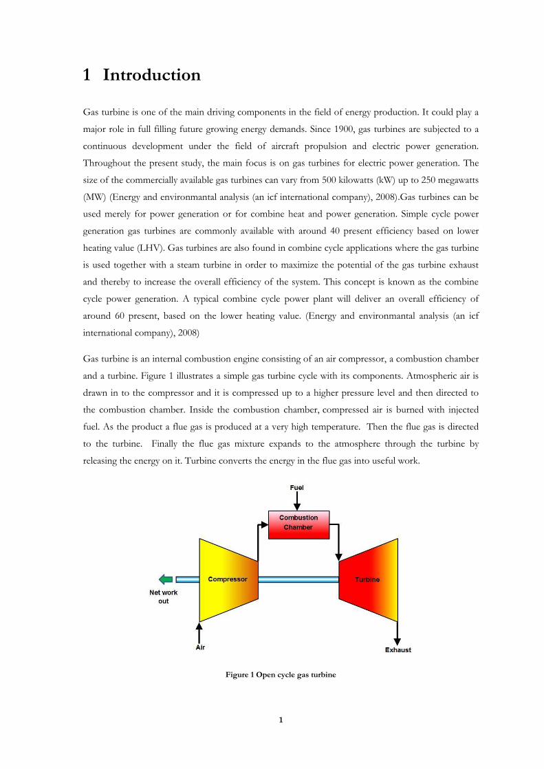
Gas turbine is an internal combustion engine consisting of an air compressor, a combustion chamber

and a turbine. Figure 1 illustrates a simple gas turbine cycle with its components. Atmospheric air is

drawn in to the compressor and it is compressed up to a higher pressure level and then directed to

the combustion chamber. Inside the combustion chamber, compressed air is burned with injected

fuel. As the product a flue gas is produced at a very high temperature. Then the flue gas is directed

to the turbine. Finally the flue gas mixture expands to the atmosphere through the turbine by

releasing the energy on it. Turbine converts the energy in the flue gas into useful work.

Figure 1 Open cycle gas turbine

2

1.1 Background

The data published by gas turbine manufactures are often found with certain exclusions due to

business reasons and thus only provide essential information for the general understanding of the

gas turbine. When referring to the manufacture’s catalogue, there are usually five main data that can

be identified for any industrially available gas turbine. Those are listed below;

Electrical power output

Overall thermal efficiency

Exhaust mass flow rate

Exhaust temperature of flue gas

Pressure ratio of the compressor

However, the important data which is essential to analyse the thermodynamic quality of a gas turbine

remains hidden. Therefore a need for such data exists among the users of gas turbines in order to be

able to compare the performances of different gas turbines.

1.2 Motivation

As a solution to the background situation described above, a program has been developed based on

the MATHCAD software to find the hidden thermodynamic properties of a gas turbine by using the

turbine catalogue data (Wettstein, 2007). That program nevertheless comes with a couple of

limitations. First and foremost it does not provide a clear problem solving procedure to the user and

hence a user will have to spend a considerable amount of time comprehending it. Having to recall

thermodynamic properties of fluids from external libraries is another limitation. This thesis work

therefore aims to develop a new program overcoming such demarcations and to develop a user

friendly graphical interface to run the program. It however uses the thermodynamic model developed

in the aforementioned MATHCAD program. The new program thereby, will be useful not only for

the industrial but also for academic purposes. It will provide more freedom for engineering students

to study and analysis gas turbines with more flexibility. Finally, this program is expected to be

incorporated into the CompEdu learning platform.

1.3 Objectives

In order to develop this new user friendly program, following objectives are met.

Develop a graphical user interface (GUI) where users can feed in a variety of input

parameters and compare the results in the same window against the input parameters.

3

A key limitation in the existing MATHCAD based program is that it can only perform

calculations for the fuel methane (CH4). The new program shall be able to accommodate for

several fuels.

Develop the program in such a way that it does not need to recall thermodynamic properties

of fluids from external libraries but use internal libraries. This will increase the versatility of

the program.

Enhance the analytical capacity compared to the existing MATHCAD program by

introducing more functions to perform detailed calculations.

Provide access for users to incorporate new functions to the program.

Perform a step by step elaboration of the calculation process for improved

comprehensibleness for users and also to make the program readily adoptable into education

platforms such as CompEdu (compedu, 2013).

Perform a detailed exergy analysis on the gas turbine by using the thermodynamic results

obtained by the programme.

4

2 Literature review

Under the subject of gas turbines, there is a vast amount of literature available regarding the topic of

gas turbines performance analysis. Most of the literature are focused on the performance variation of

gas turbines with respect to variables such as ambient temperature, ambient pressure, relative

humidity and turbine inlet temperature. The literature review revealed the fact that most published

literature refer to the Brayton cycle as the basic theoretical model for theoretical thermodynamic

analysis of gas turbines.

2.1 Basic Gas Turbine Operation

A schematic diagram of a simple cycle, single shaft gas turbine is shown in Figure 2. Air enters the

axial flow compressor through point 1 which is at ambient conditions. Then it is compressed up to a

higher pressure level. During this process there is no heat addition to the air, however the

compression of air raises the temperature. So that the compressed air at the compressor discharge is

at high pressure and temperature. The compressed air then enters the combustion chamber at point

2, where fuel is injected and combustion takes place. Either gaseous fuel (e.g. methane, natural gas,

etc.) or liquid fuels (e.g. diesel, heavy fuel) can be used in here. The combustion process occurs at

constant pressure. The combustion chamber is design to provide mixing, burning and dilution effects

to have proper combustion. The combustion product which is the flue gas leaves the combustion

chamber at very high temperature. (Brooks, 2005)

Figure 2 Simple cycle, single shaft gas turbine (Brooks, 2005)

At point 3 the flue gas enters the turbine. In the turbine section, energy of the hot gas is converted

into work. This conversion happens in two steps. In the first step, hot gases are expanding through

5

the nozzle by converting the thermal energy to the kinetic energy. Then the turbine blades are

converting this kinetic energy to mechanical work. The work delivered by the turbine blades is used

to run the compressor and the remaining power is available for useful work at the output shaft of the

turbine. As shown in the Figure 2 the output shaft can be coupled to an electrical generator to

produce electricity. After the expansion through the turbine, exhaust gas leaves the system to the

atmosphere at point 4. Still the exhaust gas is at a very high temperature and therefore has

considerable amount of energy content in it. An energy recovery unit can be used to recover this

energy for useful work. Heat recovery steam generator (HRSG) is a component which can be used to

capture the energy of exhaust gas from the gas turbine. Recovered energy can be used to run a steam

turbine and generate electricity.

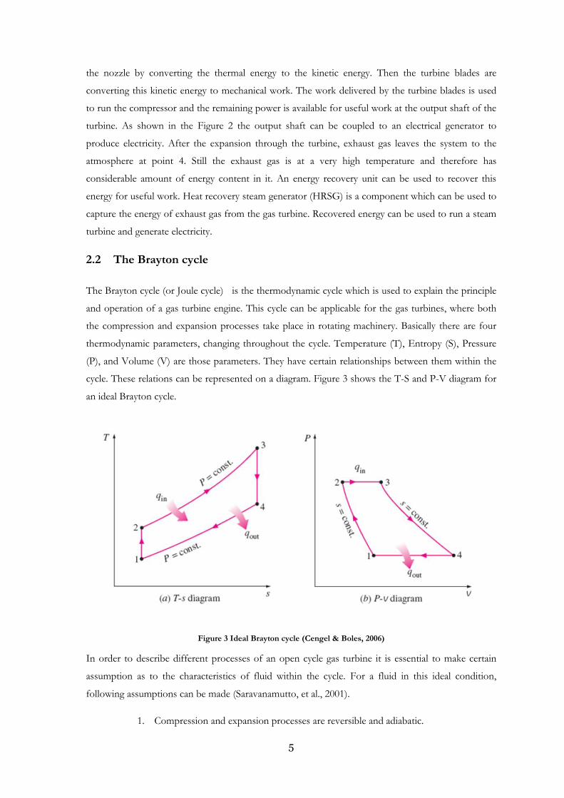
2.2 The Brayton cycle

The Brayton cycle (or Joule cycle) is the thermodynamic cycle which is used to explain the principle

and operation of a gas turbine engine. This cycle can be applicable for the gas turbines, where both

the compression and expansion processes take place in rotating machinery. Basically there are four

thermodynamic parameters, changing throughout the cycle. Temperature (T), Entropy (S), Pressure

(P), and Volume (V) are those parameters. They have certain relationships between them within the

cycle. These relations can be represented on a diagram. Figure 3 shows the T-S and P-V diagram for

an ideal Brayton cycle.

Figure 3 Ideal Brayton cycle (Cengel & Boles, 2006)

In order to describe different processes of an open cycle gas turbine it is essential to make certain

assumption as to the characteristics of fluid within the cycle. For a fluid in this ideal condition,

following assumptions can be made (Saravanamutto, et al., 2001).

1. Compression and expansion processes are reversible and adiabatic.

6

2. The change of kinetic energy of the working fluid between intake and outlet of each

component is negligible.

3. There are no pressure losses in the inlet ducting, combustion chamber, heat

exchangers, intercoolers, exhaust ducting and ducts connecting the component.

4. The working fluid has the same composition throughout the cycle and is a perfect

gas with constant specific heat.

5. The mass flow is constant throughout the cycle.

Thereby, the open cycle gas turbine which is described above can be modelled as a closed cycle

shown in Figure 3. The cycle is consists of four internally reversible processes.

1-2 Isentropic compression in the compressor

2-3 Constant pressure heat addition in the combustor

3-4 Isentropic expansion in the turbine

4-1 Constant pressure heat rejection

The following equations (equations 1 to 5) are used to describe the Brayton cycle (Saravanamutto, et

al., 2001).

Steady flow energy equation for ideal Brayton cycle is given in Equation 1, where Q and W represent

the heat and work transfers per unit mass, C is the air velocity and h is the enthalpy of fluid.

( )

(

) Equation 1

This equation can be applied separately to each component of the cycle to derive following equations

2, 3 and 4 with the assumption (2) mentioned above.

During the stage 1 to 2 ambient air get compressed through an isentropic compression process. The

amount of work done by the compressor can be calculated as follows;

( ) ( ) Equation 2

From the stage 2 to 3, compressed air is going through a constant pressure heat addition process.

Equation 3 represents the amount of heat supplied to the air during the combustion process in the

combustor.

( ) ( ) Equation 3

Finally in the turbine, hot gas is expanding through an isentropic process by releasing energy as

mechanical work. Equation 4 represents the amount of energy transfer to the turbine.

7

( ) ( ) Equation 4

With the use of above three equations, overall efficiency of the cycle can be calculated. Definition of

the efficiency for ideal gas turbine cycle is the ratio of “the network output by the system” to “the

input energy to the combustor”. Hence efficiency of the turbine can be represented as Equation 5

( ) ( ))

( )

Equation 5

2.3 Site dependent parameters

The ambient conditions are varying not only by location but also with time. Hence it is appropriate to

define a standard ambient condition. This is necessary to compare gas turbines and hence the

performance tests can be conducted in the same standard condition.

ISO Standard 3977-2 -Gas Turbines - Procurement - Part 2: Standard Reference Conditions and

Ratings, is the standard that defines the ambient conditions which can affect the inlet air density or

mass flow rates (brighthubengineering, 2013). According to the ISO standards there are three main

parameters identified as site dependent parameters. The parameters are listed below with the values

defied by ISO standard.

1. Ambient temperature 15 0C/590F

2. Relative humidity (RH) 60%

3. Ambient pressure 1.013 bar/14.7 psi

The given gas turbine performance data by the manufactures are based on these standard conditions.

When the gas turbine operates in different ambient conditions than the standard ambient conditions,

performance of the gas turbine is going to vary from standard values.

2.3.1 Ambient temperature

Ambient temperature can be simply explained as the temperature of the surrounding or the

temperature of the environment. Ambient air is used by both natural and manmade systems to

function their own cycles properly. Human body is a natural system which breath in ambient air to

absorbed oxygen for the function of human organ. In the same time manmade systems such as

internal combustion engines and gas turbines breathe air from the ambient environment for its

operation. Variation of the ambient temperature is going to change the properties of air. The

following paragraph is describing the effect of ambient temperature change on gas turbine

performance.

8

Gas turbine performance is directly affected by the change of ambient temperature. When the

ambient temperature is changed, the air density also changes correspondingly. Increase of ambient

temperature decreases the air density. Hence the mass flow rate of air is reduced. Thus the power

production of the turbine is reduced. Meanwhile the increase of ambient temperature increases the

power requirement of the compressor due to the increased air volume. Therefore more of the work

output from the turbine is used at the compressor which means the effective work output for

electricity production is affected ( Rahman, et al., 2011)

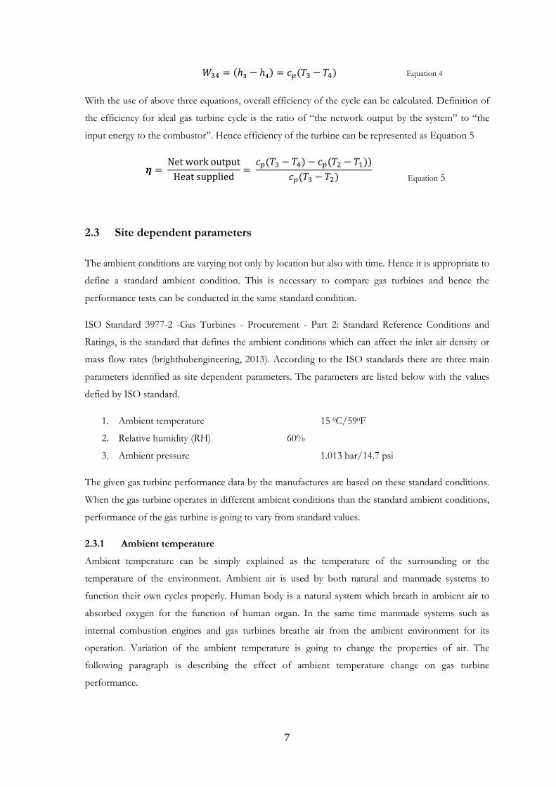
Figure 4 Effect of ambient temperature (Brooks, 2005)

Figure 4 shows the effect of ambient temperature on gas turbines. It clearly shows that the exhaust

mass flow rate, heat consumption and the power output is reducing with the increase of ambient

temperature but the heat rate of flue gas is increasing with the ambient temperature. The Y axis

indicates the variation of each factor as a percentage. 100% represents the standard ambient

conditions which are at the ambient temperature 15 0C (Brooks, 2005).

2.3.2 Relative humidity

The water content in air has a significant effect on the performance of a gas turbine because it

changes the density of the air (Brooks, 2005). Air density depends on the molecular mass of the air.

The molecular mass of water vapour (H2O) is less than the molecular mass of air. Hence higher

relative humidity or higher water content in air reduces the density of air. (wikipedia, 2013). As a

result of less density of air mass flow rate through the system is reduced. Hence power production of

the turbine also going to be reduced.

Figure 5 shows the variation of power output and the heat rate of exhaust gas with the change of

Specific humidity. Specific humidity is also a measure of water content in air. The standard relative

9

humidity of ambient air which is 60% corresponds to a value of 0.0064 in terms of specific humidity.

Y axis represents the correction factor of power output and heat rate. Power output of the turbine

reduces with the increasing water content in air nevertheless; it is evident that the effect of relative

humidity on turbine power output is significantly smaller than the effect of ambient air temperature.

Figure 5 Effect of Relative humidity (Brooks, 2005)

With the increasing size of gas turbines and the utilization of humidity for NOX control, relative

humidity has a great significance (Brooks, 2005) on it. Normally water or steam injection is used to

control the NOX production by controlling the firing temperature inside the combustion chamber.

(Brooks, 2005)

2.3.3 Ambient pressure

Ambient pressure is a site dependent parameter for the gas turbines and it changes with the

elevation/altitude. Sea level is considered as the standard elevation with a 1.013 bar pressure. With

the increase of altitude, ambient pressure gets reduced. As a result of reduced pressure,

simultaneously density of the air is also reduced. Due to the lower air density, mass flow rate through

the gas turbine cycle is reduced. Hence the output power is reduced correspondingly. The left axis of

Figure 6 shows the variation of ambient pressure with the altitude. It shows that the reduction of

ambient pressure with the increasing altitude. The zero altitude represent the see level. Right side axis

shows the power output as a correction factor. Therefore it is evident that the turbine power output

is reduced with the increasing altitude.

10

Figure 6 Altitude correction curve (Brooks, 2005)

2.4 Pressure ratio

The term pressure ratio (r) is used to represent the ratio between compressor outlet pressure and the

compressor inlet pressure. It indicates the compressibility of the compressor. In an ideal cycle,

ambient air enters the compressor intake without a pressure drop. Then it gets compressed and

leaves the compressor at a higher pressure. As shown in Figure 3(a) same pressure is maintained till

the inlet to the turbine while heat is added through the combustor at this constant pressure. Finally

pressurized hot gas expands to the ambient environment through the turbine. Hence pressure ratio

across the turbine and compressor is the same for ideal gas turbine cycle. Pressure ratio ( ) can be

presented in the Equation 21 6 as follows;

Equation 6

Due to the compression process happening through the compressor, air temperature increases from

the inlet temperature to a higher temperature. Equation 7 is representing the temperature and

pressure relationship for isentropic compression. Gamma ( ) represents the heat capacity ratio of the

working fluid (gas). In this case air acts as the working fluid.

(

)

( )

Equation 7

Same equation can be used to represent the turbine expansion process as follows.

11

(

)

( )

Equation 8

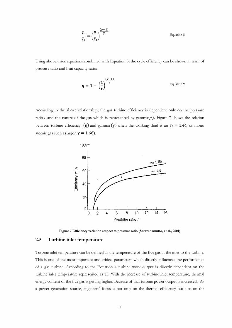
Using above three equations combined with Equation 5, the cycle efficiency can be shown in term of

pressure ratio and heat capacity ratio;

(

)

( )

Equation 9

According to the above relationship, the gas turbine efficiency is dependent only on the pressure

ratio and the nature of the gas which is represented by gamma( ). Figure 7 shows the relation

between turbine efficiency ( ) and gamma ( ) when the working fluid is air ( ), or mono

atomic gas such as argon ).

Figure 7 Efficiency variation respect to pressure ratio (Saravanamutto, et al., 2001)

2.5 Turbine inlet temperature

Turbine inlet temperature can be defined as the temperature of the flue gas at the inlet to the turbine.

This is one of the most important and critical parameters which directly influences the performance

of a gas turbine. According to the Equation 4 turbine work output is directly dependent on the

turbine inlet temperature represented as T3. With the increase of turbine inlet temperature, thermal

energy content of the flue gas is getting higher. Because of that turbine power output is increased. As

a power generation source, engineers’ focus is not only on the thermal efficiency but also on the

12

specific work output ( ) of the turbine. Useful work output of the turbine can be represented as the

difference of turbine power output and compressor power consumption.

( ) ( ) Equation 10

To understand the power production ability with respect to turbine inlet temperature, the Equation

10 can be further analysed. Equation 10 can be represented in terms of pressure ratio and

gamma( ) , which show the relations of turbine power output to pressure ratio and gamma.

(

( )

) ( ( ) ) Equation 11

Where “t” represents the ratio of T3/T1; and T1 is the ambient temperature and T3 is the turbine inlet

temperature. With the increase of the turbine inlet temperature, specific work output of the turbine is

increased. For each turbine inlet temperature, there is an optimum compressor pressure ratio. The

reason behind this is the power consumption of the compressor. Compressor consumes more power

when it needs to have higher pressure ratios. Because of that compressor pressure ratio has an

optimum value to maximize the specific power output. These relationships can be plotted on a

graph to see the variation of specific work output of turbine with the changing pressure ratios ( )

and “t”. Figure 8 represents the variation of specific power with respect to the parameters mention

above.

Figure 8 Variation of specific work output (Saravanamutto, et al., 2001)

13

2.6 Efficiency of the components

Individual components of the gas turbine play a major role in power output and in the plant’s overall

efficiency. The compressor, turbine, combustion chamber and electrical generator are the main

components of the cycle. By reducing the inefficiencies in individual components, plant efficiency

can be increased by a considerable amount. Among the main components, compressor and turbine

can be identified as most critical components. Isentropic efficiency and the polytropic efficiency are

two important factors related to the compressor and the turbine.

2.6.1 Isentropic efficiency

Many engineering processes or devices such as compressors, turbines, pumps, nozzles and diffusers

are related to work transfer processes. In ideal situation these systems work as adiabatic and internally

reversible systems. Hence these processes can be defined as isentropic process. An isentropic process

is a constant entropy process and the entropy does not change throughout the process. In reality

these processes are not internally reversible because of the friction associated to the process. Due to

the fact that the actual processes are not isentropic and hence there is an entropy change through the

process. Therefore the thermodynamic properties such as temperature and specific enthalpy are

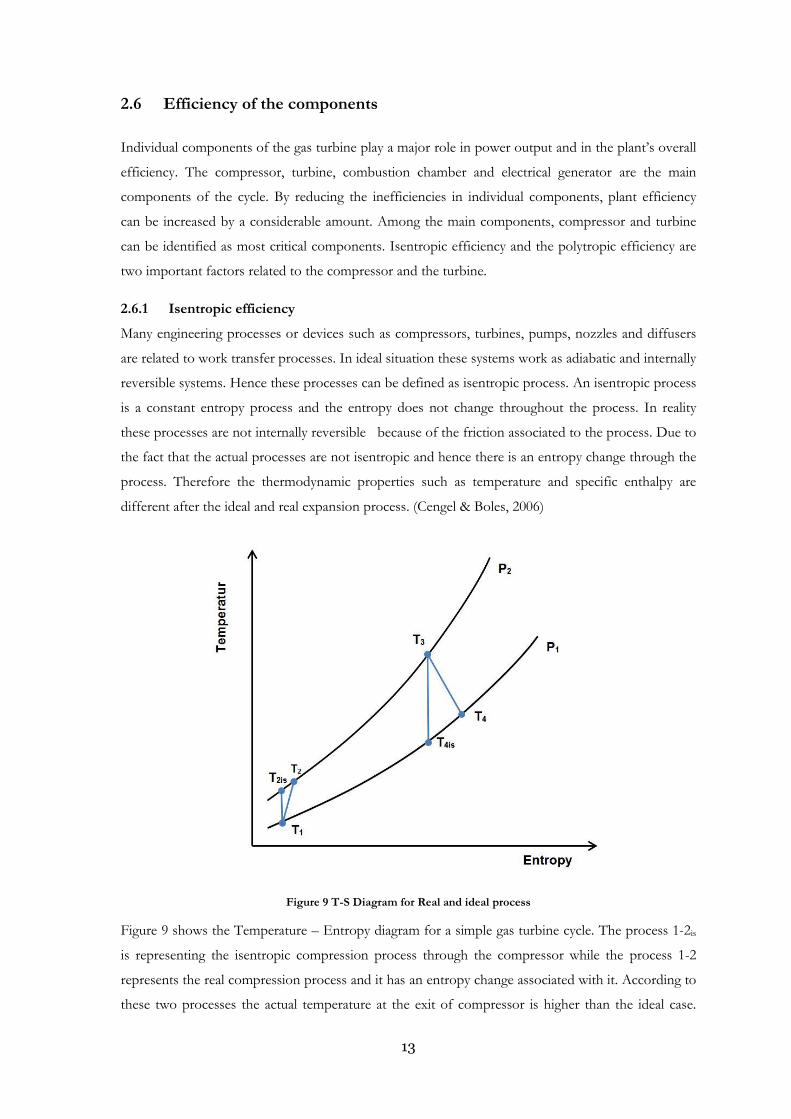
different after the ideal and real expansion process. (Cengel & Boles, 2006)

Figure 9 T-S Diagram for Real and ideal process

Figure 9 shows the Temperature – Entropy diagram for a simple gas turbine cycle. The process 1-2is

is representing the isentropic compression process through the compressor while the process 1-2

represents the real compression process and it has an entropy change associated with it. According to

these two processes the actual temperature at the exit of compressor is higher than the ideal case.

14

Hence the energy requirement to compress a fluid for a given pressure ratio is higher in the actual

process than the ideal case. Isentropic efficiency of the compressor can be defined based on the

actual and ideal energy requirements for the compression process as follows;

Equation 12

Ideal and actual turbine expansion processes are also represented in the same T-S diagram in Figure

9. Process 3-4is is the isentropic expansion process with constant entropy and the process 3-4 is the

actual turbine expansion process with an entropy change. The real turbine outlet temperature is

higher than the ideal case. So that the energy change or extraction through the turbine is going to be

less than the ideal case. Isentropic efficiency of the turbine can be defined based on the actual and

ideal energy change of the fluid through the expansion process. Equation 2113 is representing the

definition of isentropic efficiency of a turbine.

Equation 13

To find the compressor isentropic efficiency, Equation 12 can be modified as follows;

( )

( ) Equation 14

( )( ) Equation 15

( )[( )

( ) ] Equation 16

Similarly, Equation 13 can be used to show the turbine isentropic efficiency as follows;

( )

[ ( ⁄ )( ) ]

Equation 17

15

According to the Equation 16 and Equation 17, isentropic efficiency of the compressor and the

turbine are dependent on the compressor pressure ratio. In fact it is found out that the isentropic

efficiency of the compressor decreases and isentropic efficiency of the turbine increases

with the increase of compressor pressure ratio (Saravanamutto, et al., 2001) When performing a

calculation or a simulation with various pressure ratios it is better to assume a fixed typical value for

and for hence it helps to simplify the calculations. If not relevant isentropic efficiency

values should be changed according to the pressure ratios used in the calculation.

2.6.2 Polytropic efficiency

An axial flow compressor consists of a number of intermediate pressure stages to achieve the final

pressure ratio. The definition of isentropic efficiency can be applied to each intermediate pressure

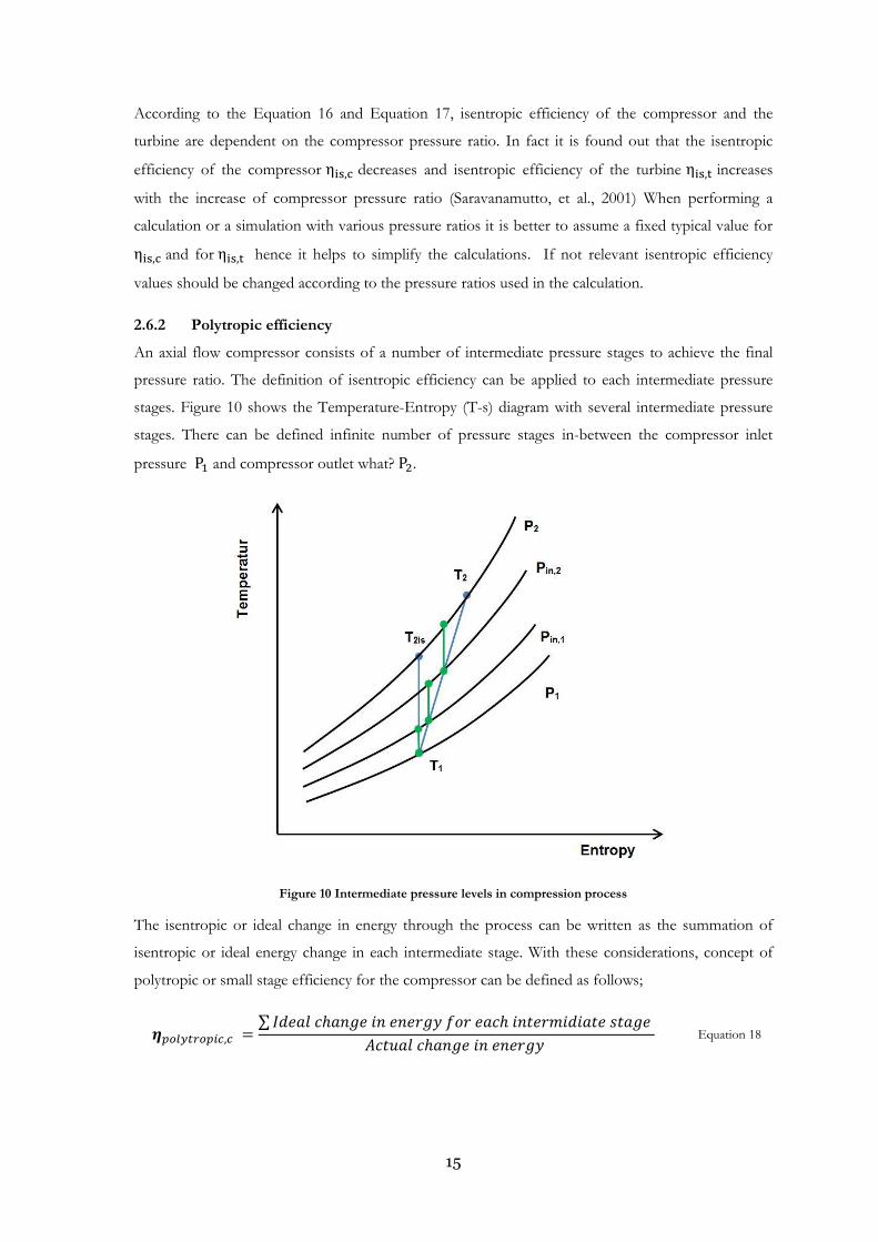
stages. Figure 10 shows the Temperature-Entropy (T-s) diagram with several intermediate pressure

stages. There can be defined infinite number of pressure stages in-between the compressor inlet

pressure and compressor outlet what? .

Figure 10 Intermediate pressure levels in compression process

The isentropic or ideal change in energy through the process can be written as the summation of

isentropic or ideal energy change in each intermediate stage. With these considerations, concept of

polytropic or small stage efficiency for the compressor can be defined as follows;

∑

Equation 18

16

The vertical distance between a pair of constant pressure lines in the T-s diagram, increases as the

entropy increases (Saravanamutto, et al., 2001). This shows as well in the Figure 10. Hence the

temperature difference of each intermediate stage increasing with the increase of entropy. Increase of

the temperature difference represents the increase of energy change in between the intermediate

pressure stages. Hence summation of ideal energy change in intermediate stages is going to be higher

than the ideal change in energy in-between compressor inlet and outlet. By considering this change of

energy in the Equation 12 and Equation 18 it shows that the polytropic efficiency of the compressor

( ) is greater than the isentropic efficiency of the compressor ( )

The same argument can be used to define the polytropic efficiency of the turbine as follows;

∑ Equation 19

Expansion process of the turbine is also happening through several intermediate stages. Hence the

ideal change in energy can be calculated for each stage. The summation of this intermediate ideal

energy changes is higher than the ideal energy change mention in the Equation 13. Due to that reason

the polytropic efficiency of the turbine ( ) is lesser than the isentropic efficiency of the

turbine ( )

2.7 Conclusion for the literature review

The topics discussed under the literature review are basic theories and concepts behind the gas

turbine cycles. It is helpful to understand the basic thermodynamic equations and terms related to the

gas turbine performance data analysis. Clear understandings of those facts are useful to recognize and

explain the results obtained by the gas turbine data analysis program.

Gas turbines used in the industry are having slight differences than the ideal gas turbine cycle

discussed in literature review chapter. Those conditions are not discussed in the literature review

chapter. As an example there are some pressures losses taking place at the air inlet to the compressor

and there are some heat extractions taking place in the turbine. Specially cooling air extraction lines

start from the compressor which bypass the combustion chamber and directed to the turbine blades

for cooing purposes. Effects of those differences were taken in to consideration, in developing the

program to determine the performance data of a gas turbine cycle.

17

3 Methodology

As mentioned abstract, there exists a MATHCAD program to find the hidden thermodynamic

properties of a gas turbine using the given data by the turbine manufacture. The task of this thesis is

to create a new program by improving and adding new features to the existing program. As a starting

point the existing program is studied together with related literature

3.1 Analysis of previous works

The existing MATHCAD program to analyse the simple cycle gas turbine and to find the hidden

thermodynamic parameters is made by Professor Hans E. Wettstein from ETH, Zürich Switzerland

MATHCAD program

MATHCAD is an industry standard calculation software for technical professionals, educators and

college students. MATHCAD is as versatile and powerful as the programming language (MathSoft,

2000). This programme was formulated to calculating hidden data of an open cycle gas turbine with

the use of available catalogue data and with some realistic assumptions.

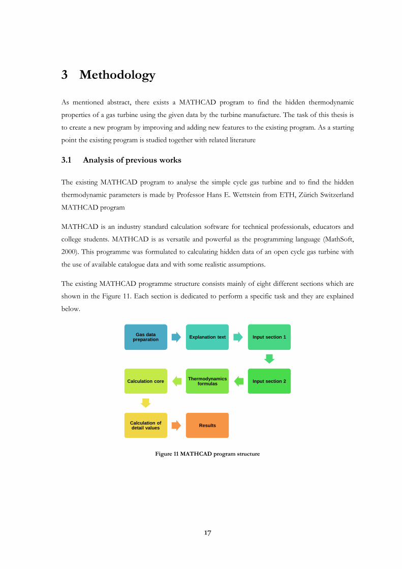
The existing MATHCAD programme structure consists mainly of eight different sections which are

shown in the Figure 11. Each section is dedicated to perform a specific task and they are explained

below.

Figure 11 MATHCAD program structure

Gas data preparation

Explanation text Input section 1

Input section 2 Thermodynamics

formulas Calculation core

Calculation of detail values

Results

18

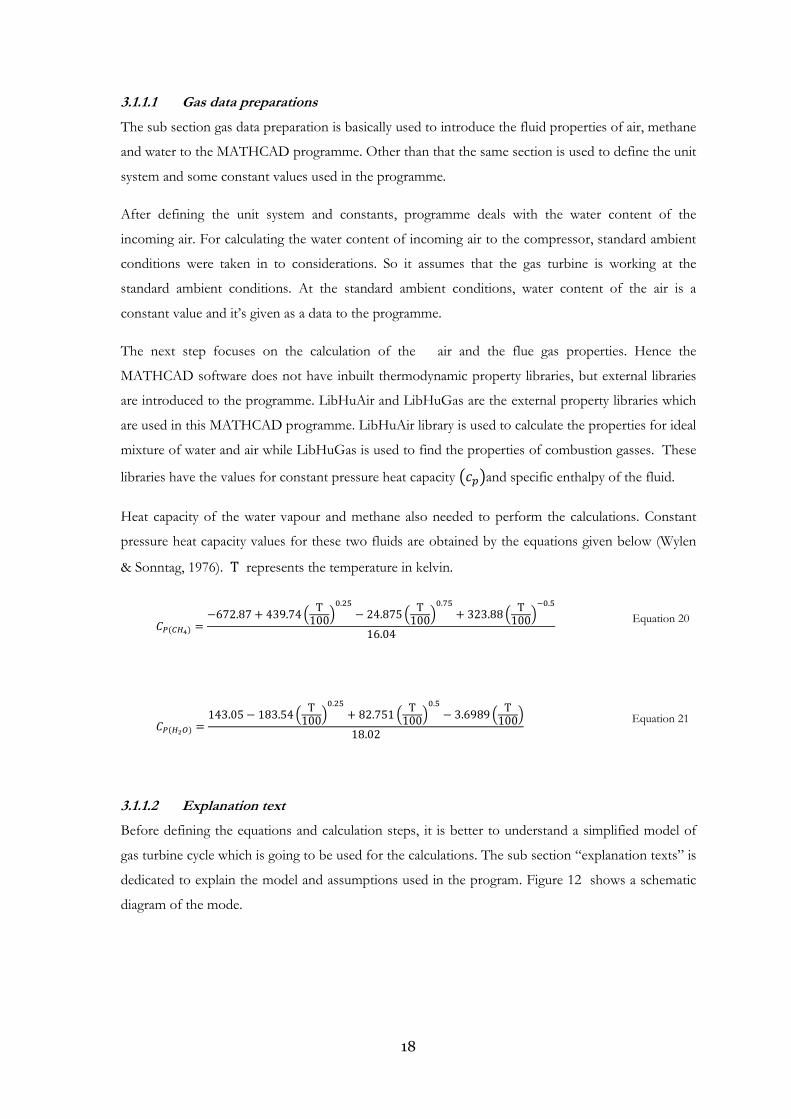
3.1.1.1 Gas data preparations

The sub section gas data preparation is basically used to introduce the fluid properties of air, methane

and water to the MATHCAD programme. Other than that the same section is used to define the unit

system and some constant values used in the programme.

After defining the unit system and constants, programme deals with the water content of the

incoming air. For calculating the water content of incoming air to the compressor, standard ambient

conditions were taken in to considerations. So it assumes that the gas turbine is working at the

standard ambient conditions. At the standard ambient conditions, water content of the air is a

constant value and it’s given as a data to the programme.

The next step focuses on the calculation of the air and the flue gas properties. Hence the

MATHCAD software does not have inbuilt thermodynamic property libraries, but external libraries

are introduced to the programme. LibHuAir and LibHuGas are the external property libraries which

are used in this MATHCAD programme. LibHuAir library is used to calculate the properties for ideal

mixture of water and air while LibHuGas is used to find the properties of combustion gasses. These

libraries have the values for constant pressure heat capacity ( )and specific enthalpy of the fluid.

Heat capacity of the water vapour and methane also needed to perform the calculations. Constant

pressure heat capacity values for these two fluids are obtained by the equations given below (Wylen

& Sonntag, 1976). represents the temperature in kelvin.

( ) (

)

(

)

(

)

Equation 20

( ) (

)

(

)

(

)

Equation 21

3.1.1.2 Explanation text

Before defining the equations and calculation steps, it is better to understand a simplified model of

gas turbine cycle which is going to be used for the calculations. The sub section “explanation texts” is

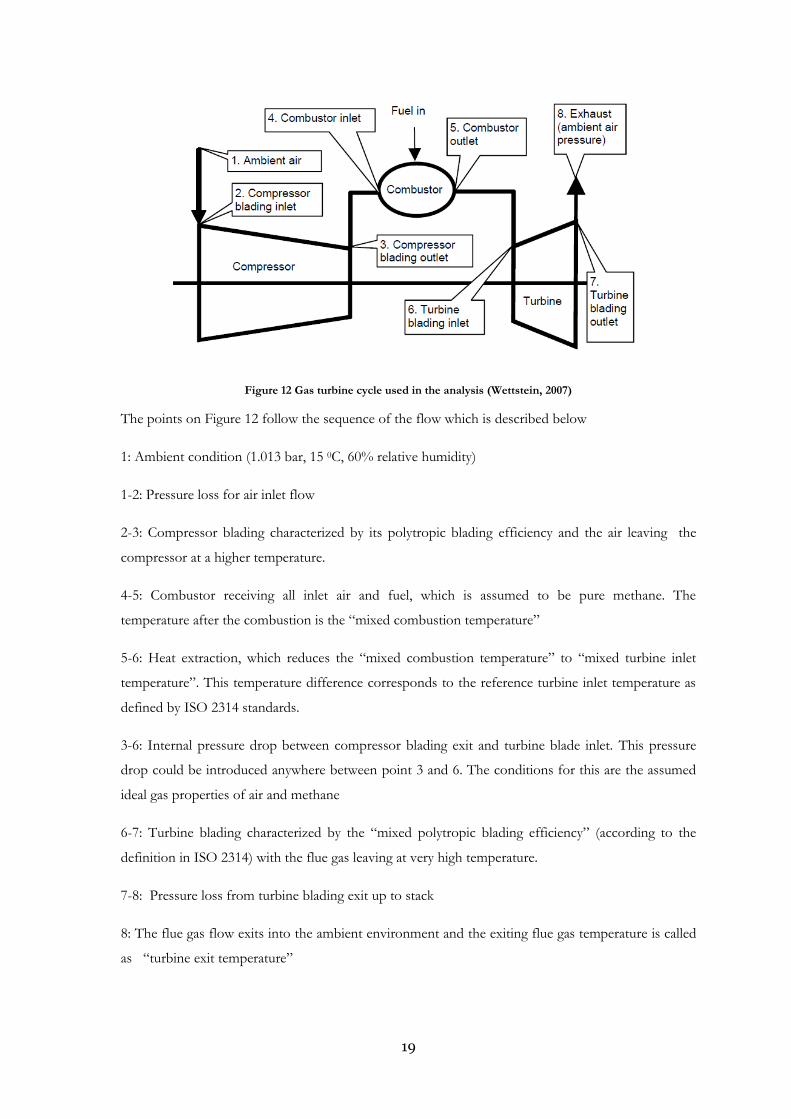
dedicated to explain the model and assumptions used in the program. Figure 12 shows a schematic

diagram of the mode.

19

Figure 12 Gas turbine cycle used in the analysis (Wettstein, 2007)

The points on Figure 12 follow the sequence of the flow which is described below

1: Ambient condition (1.013 bar, 15 0C, 60% relative humidity)

1-2: Pressure loss for air inlet flow

2-3: Compressor blading characterized by its polytropic blading efficiency and the air leaving the

compressor at a higher temperature.

4-5: Combustor receiving all inlet air and fuel, which is assumed to be pure methane. The

temperature after the combustion is the “mixed combustion temperature”

5-6: Heat extraction, which reduces the “mixed combustion temperature” to “mixed turbine inlet

temperature”. This temperature difference corresponds to the reference turbine inlet temperature as

defined by ISO 2314 standards.

3-6: Internal pressure drop between compressor blading exit and turbine blade inlet. This pressure

drop could be introduced anywhere between point 3 and 6. The conditions for this are the assumed

ideal gas properties of air and methane

6-7: Turbine blading characterized by the “mixed polytropic blading efficiency” (according to the

definition in ISO 2314) with the flue gas leaving at very high temperature.

7-8: Pressure loss from turbine blading exit up to stack

8: The flue gas flow exits into the ambient environment and the exiting flue gas temperature is called

as “turbine exit temperature”

20

The programme consists of some simplifications and assumptions as well. Above topics are also

discussed in detail within the present section “Explanation text”. This is the section where the

program explains that the calculations are limited to the use of pure methane as the fuel. It is also

assumed that the value of the specific heat capacity of flue gas is as same as the value of air-methane

mixture. That is because the reaction of pure methane with oxygen is happening without a volume

change (Wettstein, 2006). .

The same “Explanation text” section of the MATHCAD programme also mentions that for

simplification of the thermodynamic equations, constant pressure specific heat capacity is taken into

consideration. Pressure dependency of the heat capacity (real gas effect) is not considered throughout

the program.

3.1.1.3 Input section 1

Input section 1 is developed so that the user can insert the general data required to perform the

calculations. Then these values remain fixed throughout the program. In this section there are eleven

parameters taken in to consideration. They are listed in Table 1 with the values for a particular gas

turbine which is used for the calculations. These values can be changed by the users depending on

the gas turbine which is going to be analysed.

Table 1 parameters in the input section 1

Input parameter Value

Relative inlet pressure loss until blading 0.01

Relative outlet pressure loss (blading to ambient) 0.013

Relative internal pressure loss (shall include the compressor

diffuser loss)

0.065

Compressor relative diffuser loss (related to plenum pressure) 0.02

H2O content of Air at 15°C with 60% humidity

related to dry air:

0.0063

Ambient pressure: 1.013 bar

Ambient temperature: 288 K

Lower heating value of the fuel (methane): 50 MJ/kg

Fuel gas inlet temperature: 288 K

Electrical efficiency 0.986

Mechanical efficiency 0.995

21

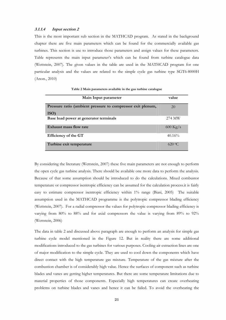
3.1.1.4 Input section 2

This is the most important sub section in the MATHCAD program. As stated in the background

chapter there are five main parameters which can be found for the commercially available gas

turbines. This section is use to introduce those parameters and assign values for these parameters.

Table represents the main input parameter’s which can be found from turbine catalogue data

(Wettstein, 2007). The given values in the table are used in the MATHCAD program for one

particular analysis and the values are related to the simple cycle gas turbine type SGT6-8000H

(Anon., 2010)

Table 2 Main parameters available in the gas turbine catalogue

Main Input parameter value

Pressure ratio (ambient pressure to compressor exit plenum,

ISO)

20

Base load power at generator terminals 274 MW

Exhaust mass flow rate 600 Kg/s

Efficiency of the GT 40.16%

Turbine exit temperature 620 0C

By considering the literature (Wettstein, 2007) these five main parameters are not enough to perform

the open cycle gas turbine analysis. There should be available one more data to perform the analysis.

Because of that some assumption should be introduced to do the calculations. Mixed combustor

temperature or compressor isentropic efficiency can be assumed for the calculation process.it is fairly

easy to estimate compressor isentropic efficiency within 1% range (Biasi, 2005) The suitable

assumption used in the MATHCAD programme is the polytropic compressor blading efficiency

(Wettstein, 2007). For a radial compressor the values for polytropic compressor blading efficiency is

varying from 80% to 88% and for axial compressors the value is varying from 89% to 92%

(Wettstein, 2006)

The data in table 2 and discussed above paragraph are enough to perform an analysis for simple gas

turbine cycle model mentioned in the Figure 12. But in reality there are some additional

modifications introduced to the gas turbines for various purposes. Cooling air extraction lines are one

of major modification to the simple cycle. They are used to cool down the components which have

direct contact with the high temperature gas mixture. Temperature of the gas mixture after the

combustion chamber is of considerably high value. Hence the surfaces of component such as turbine

blades and vanes are getting higher temperatures. But there are some temperature limitations due to

material properties of those components. Especially high temperatures can create overheating

problems on turbine blades and vanes and hence it can be failed. To avoid the overheating the

22

solution is to cool the component. So that the cooling air extraction lines are introduced as a

solution.

In the real gas turbine arrangement there are some air extractions from air compressor to use for

cooling purposes which are discussed above. This cooling air bypasses the combustion chamber and

directed to the turbine to cool down the turbine components. According to the MATHCAD

program there exist two main cooling lines existing and they are given as a ratio to the inlet air mass

flow rate.

1. Cooling air ratio of vane 1

2. Cooling air ratio downstream vane 1

In the input section 2, users can introduce the values for cooling air ratio vane 1 and downstream

vane 1 to the MATHCAD program.

3.1.1.5 Thermodynamics formulae

This section is used to define some of the thermodynamic equation in the MATHCAD programme.

There are eight different thermodynamic equations presented in this section. All the formulas are

written by using MATHCAD notations and most of the equations have integral functions as well.

These formulas are used to calculate the hidden thermodynamic parameters based on the model

explained by Figure 12. Descriptions of the formulas are written below and detailed description can

be found in the coming chapters.

1. Polytropic compressor blading efficiency as a function of pressure ratio, gas data ambient

temperature and exit temperature.

2. Specific compressor power related to the dry air mass flow rates.

3. Ratio of methane to dry air; this is an energy balance to the air fuel mixture by considering

the incoming and outgoing streams to the combustion chamber.

4. Heat extraction; there are some heat extractions happen due to the presence of external

cooling lines.(Steam cooling lines or external cooling air lines.)

5. Polytropic turbine blading efficiency as a function of pressure ratio, gas data, turbine inlet

temperature and turbine exit temperature.

6. Specific power of the turbine blading.

7. Specific electric net turbine power.

8. Net gas turbine efficiency.

This sub section does not perform any calculations but the related formula’s for the calculations

mentions above are stored in the programme. These equations are used in appropriate way to solve

the unknowns at the latter part of the programme.

23

3.1.1.6 Calculation core

The sub sections discussed above are used to define the main equations, to introduce all the input

parameters and to include the assumptions required for the programme to calculate unknown

thermodynamic parameters. All the input parameters are analysed within the calculation core section.

The calculations are carried out according to the simplified model discussed in the section

“explanation text”. According to the model it is assume that all the ambient air mass entered to the

compressor inlet is going through the combustion chamber and then expand to the ambient

environment through the turbine.

There are some additional equations required to solve the unknown parameters because there were

not enough number of equations which is already defined in previous sections. To full fill that

requirement some extra equations are introduced to the programme. As an example energy balance

to the turbine is introduce to the program.

Then all the required input parameters and equations can be used to precede the calculations by using

MATHCAD program. As a result of the calculations, several number of unknown or hidden gas

turbine thermodynamic parameters can be calculated. Some of the outcomes are listed below.

1. Compressor exit temperature

2. Specific power of the compressor blading

3. Mixed combustor temperature

4. Mixed turbine inlet temperature

5. Fuel to air ratio

6. Heat extraction from combustor

7. Specific power of the turbine blading

8. Polytropic blading efficiency.

3.1.1.7 Calculation of detail values

This section is a continuation of the calculation core. In the section above “calculation core”, basic

concern is to calculate the main important parameters which directly explain the gas turbine

behaviour. The parameters required for detail descriptions of the gas turbine are calculated separately

in this section. To achieve those parameters, set of equations are introduced in to the programme in

the section “calculation of detail values”

The effect of cooling air lines which bypass the combustion chamber and directed to the turbine is

taken in to consideration for some of the calculations carried out in this section. Mixed combustor

temperature which is calculated above is not considering the existence of cooling air lines. But the

combustor exit temperature calculated with in this section is considering the cooling air lines. Due to

the air extraction from the compressor, actual mass flow rate through the combustion chamber is less

than the ideal gas turbine cycle. But the amount of fuel injected to the combustion chamber remains

24

unchanged. Hence due to the less mass flow rate the “combustor exit temperature” increases more

than the value of “mixed combustion temperature” to maintain the energy balance across combustor.

Vane exit temperature is another unknown parameter which considers the effect of cooling air lines

when the calculations are carried out. The vane exit temperature represents the temperature of the

gas mixture directed to the first turbine blade. The value of vane exit temperature is higher than the

mixed turbine inlet temperature which is calculated in the section above. The reason behind is that

the consideration of cooling air line for the calculations. Due to the cooling mass flow rate of

downstream vane 1, actual mass flow rate through the first turbine blade is less than the ideal case.

To have the same energy content with less mass flow rate, vane exit temperature is getting higher

value than mixed turbine inlet temperature.

Gas turbines are emitting large amount of carbon dioxide (CO2) and some amount of other harmful

gases such as nitrogen oxides (NOx) to the atmosphere. Because of that the concern about

environmental effect by the gas turbines are very important. Composition of the harmful elements in

the flue gas can show a clear picture about the environmental effect by the gas turbine. Hence flue

gas analysis carried out to find the composition of the exhaust gas which is leaving the system. Basic

flue gas analysis is carried out with the available data by assuming complete combustion of fuel.

Lists of parameters calculated at this section are given below;

1. Dry air mass flow rate

2. Humid air inlet mass flow

3. Fuel mass flow rate

4. Compressor power

5. Mechanical turbine power

6. Exhaust heat flow

7. Combustor outlet temperature

8. Vane outlet temperature

9. Isentropic efficiency of turbine and compressor.

10. Carbon dioxide (CO2) production

11. Oxygen (O2) percentage in exhaust gas

12. Nitrogen oxides (NOx) in the exhaust gas

3.1.1.8 Results

This is the last section of the programme and it is dedicated to present all the parameters related to

gas turbine which are considered for the calculations. At the end of this section, MATHCAD

programme generate a table of results with the calculated values for unknown variables. It includes

not only the hidden thermodynamic parameters which are expected to be found out by the

programme but also the input parameters related to the gas turbine. Table 3 represents the result

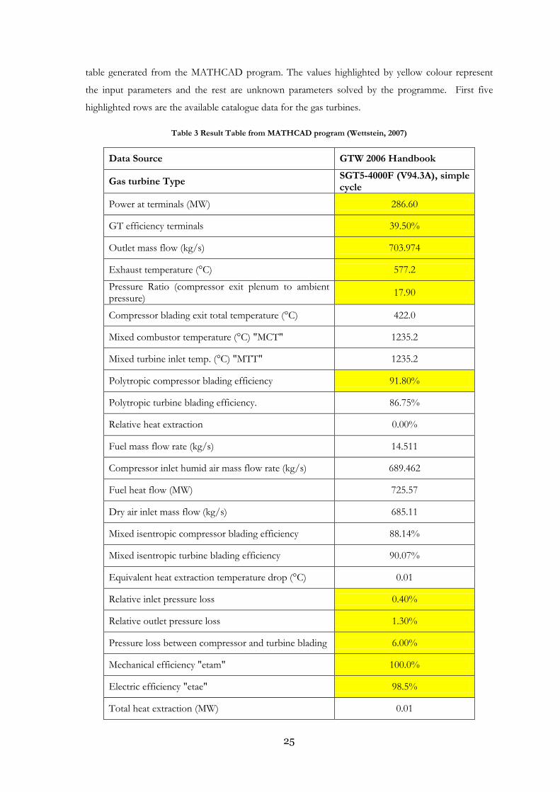
25

table generated from the MATHCAD program. The values highlighted by yellow colour represent

the input parameters and the rest are unknown parameters solved by the programme. First five

highlighted rows are the available catalogue data for the gas turbines.

Table 3 Result Table from MATHCAD program (Wettstein, 2007)

Data Source GTW 2006 Handbook

Gas turbine Type SGT5-4000F (V94.3A), simple cycle

Power at terminals (MW) 286.60

GT efficiency terminals 39.50%

Outlet mass flow (kg/s) 703.974

Exhaust temperature (°C) 577.2

Pressure Ratio (compressor exit plenum to ambient pressure)

17.90

Compressor blading exit total temperature (°C) 422.0

Mixed combustor temperature (°C) "MCT" 1235.2

Mixed turbine inlet temp. (°C) "MTT" 1235.2

Polytropic compressor blading efficiency 91.80%

Polytropic turbine blading efficiency. 86.75%

Relative heat extraction 0.00%

Fuel mass flow rate (kg/s) 14.511

Compressor inlet humid air mass flow rate (kg/s) 689.462

Fuel heat flow (MW) 725.57

Dry air inlet mass flow (kg/s) 685.11

Mixed isentropic compressor blading efficiency 88.14%

Mixed isentropic turbine blading efficiency 90.07%

Equivalent heat extraction temperature drop (°C) 0.01

Relative inlet pressure loss 0.40%

Relative outlet pressure loss 1.30%

Pressure loss between compressor and turbine blading 6.00%

Mechanical efficiency "etam" 100.0%

Electric efficiency "etae" 98.5%

Total heat extraction (MW) 0.01

26

Relative heat balance mismatch 8,1E-07

Cooling air ratio of vane 1 8.00%

Cooling air ratio downstream of vane 1 12.00%

Combustor outlet temperature, °C 1404.5

Vane outlet temperature, °C 1329.0

Fuel to dry air ratio 2.12%

Mole fraction of fuel in dry air 3.69%

Oxygen mass fraction in exhaust air 12.99%

CO2 mass fraction in exhaust air 5.67%

CO2 exhaust flow in kg/s 39.91

Overall equivalence ratio of combustion (1/lambda) 36.44%

Exergetic efficiency of the GT 89.28%

NOx ppm in exhaust corrected to 15%O2 25.0

Specific NOx production, kg/GT-MWh 0.282

Specific CO2 production, kg/GT-kWh 0.501

Fuel gas delivery temperature to GT in °C 15.00

Ambient temperature in °C 15

MATHCAD program allows opening the result table as a format of Microsoft Excel work sheet.

27

3.1.2 Review of the MATHCAD program

For the better understanding of the work, thorough study has been carried out of the MATHCAD

programme and the related documents such as Compedu chapter for the MATHCAD program. It is

considered important to understand the existing programme before developing new programme.

After the study the capabilities and limitations of the existing programme has been found out. As

well as some of the drawbacks related to the Mathcad programme can be identified, which are

explained below.

3.1.2.1 Lack of knowledge about the MATHCAD software by the user

The programme is used for educational purposes. Hence students should know the procedure or the

calculation method used by the MATHCAD programme .To understand the programme very well,

users should have a better understanding of the MATHCAD software, its behaviours and functions

as well. But most of the users are not familiar with the MATHCAD software. Those users will get

troubles since the first stage when they started to work with the programme. Hence lack of

knowledge about the MATHCAD software is a one of major drawback for the users to use the

programme.

3.1.2.2 Graphical user interface not present in the MATHCAD software

The MATHCAD software does not have features to create a graphical user interface. Hence the

programme based on MATHCAD used the same window which used to define the variables,

equations and explanations to insert the input variables. The users must search throughout the input

section 1 and the input section 2 to figure it out the variables for input parameters. This can confuse

the new users to the programme. The results appear in the last section of the programme as a

tabulated manner. If the users want to do a sensitivity analysis by varying input data, they want to go

up and down in between the input sections and result section. So that the absence of graphical user

interfaces make more troubles to the users.

3.1.2.3 Difficulties to understand the problem solving procedure

Equations presentenced in the MATHCAD programme body are not arranged in an appropriate

order. Equations can be found in four different sub sections which are gas data preparation,

thermodynamic formulas, calculation core and calculation of detail values. Because of that user can

not follow the flow of equations easily. They want to switch in-between the sub sections of the

programme mention above to find the connection among the various equations. So that the normal

users or specially the students who study about the programme must spend more time to understand

the programme.

3.1.2.4 Use of external library

The section of gas data preparation includes some external libraries. These libraries are used to

generate the gas data properties required for the calculations of constant pressure heat capacity

28

( )and specific enthalpy values. LibHuAir and LibHuGas are the external libraries which are used

in this program. Other than that there are some equations also presented in the same section to

generate gas properties for water vapour and methane. Also there is a table of constant pressure heat

capacity values for air and a graph which gives a heat capacity value for several pressure levels present

in the same section. User of the programme can be easily confused with the number of different

libraries and equations defined for the fluid property calculations. They cannot easily identify the

difference of each library and where are they going to be used within the programme. Even it is

much difficult to find a detail description about the external library functions used in the programme.

3.1.2.5 Comments in the program body is not clear enough

During the study some comments or small descriptions can be found out throughout the programme

body. Sometimes it helps to understand the steps of the each section. But in several places the

comments create some confusion to the users. Especially in the section of gas data preparation, users

can be easily confused with the comments included in it. As an example there is a comment regarding

the composition vector and the user cannot understand the meaning of this without going through

the description of LibHuGas library.

3.1.2.6 Limitations of the programme

The existing MATHCAD programme has its own limitations due to some reasons. Simple cycle gas

turbines can be analysed by the programme. But the analysis can be carried out only for the gas

turbines that run with methane as the fuel. It is harder to rearrange the programme for other types of

fuels since the fluid properties cannot be easily introduced to the programme as the programme does

not have own inbuilt library for fluid properties

By considering the above facts, for new user it is very hard to use the existing MATHCAD

programme to find the hidden thermodynamic parameters of a gas turbine . Especially when the

users are not familiar with the programme, they can make some errors or mistakes where entering the

input data. Users may enter part of the input data and rest of the input data stay same in previous

values which entered to the programme in the past. This can easily happen due to the difficulty of

finding the input data in the same section. Hence the answers for hidden thermodynamic parameters

can be inaccurate.

The users who have the better understand about the programme and have an idea about expected

thermodynamic properties from the programme can analysis the results. By considering some of the

results they can identify accuracy of the calculation. Turbine polytropic efficiency and heat extraction

temperature drop can be used for that purpose. Polytropic efficiency of the turbine should be

typically in the range of 83% to 88 % (remarks from the MATHCAD program). If the result for

turbine polytropic efficiency is not within the range mention above, it is an indication for an error in

the input data.

29

Results for heat extraction temperature drop should be less than 1 K if the relevant gas turbine does

not have external heat extractions. Also the value should be positive. Hence the heat extraction

temperature drop can also be used to check the accuracy of the results. If the results for polytropic

turbine efficiency or heat extraction temperature drop are not with in the ranges users must

crosscheck each and every input data to the programme. Exhaust mass flow rate, mechanical

efficiency and electrical efficiency are the main input data which can create inaccurate results.

3.2 Suggestions for the improvements

The MATHCAD programme to analysis hidden gas turbine thermodynamic properties is working

properly for the simple gas turbines with methane as a fuel. But for the users who do not have good

experience and understanding about the MATHCAD software faces difficulties and it is a major

drawback of the programme. According to the chapter “Review of the Mathcad program”, it is a

requirement to modify the existing program to make it more users friendly. There are several

suggestions that can be proposed to improve the existing MATHCAD program or to consider when

developing a new program with different software.

3.2.1 Graphical user interface

Most of the users of the program will use this as a calculation tool to generate the hidden

thermodynamic parameters by using the existing gas turbine catalogue data. Because of that they

might be not much interested in the programme codes and the way of arranging the equations. If

programme can provide the facility to insert the input data and see the results in the same window, it

will be very attractive to the users. Then they can directly access that window without going

throughout the programme body. This will allow changing the inputs and seeing the variation of

output parameters within a short period of time.

Graphical user interface provide a solution for the fact discussed above. But MATHCAD software

does not support for graphical user interface. There are some software’s which can provide the

facility to create a graphical user interface. Engineering Equation Solver (EES) is one of the

programme supports to create graphical user interface.

3.2.2 Well organized programme structure

The programme is going to be used for educational purpose. Hence students who are working with

the programme for study purposes must have the freedom to see the core of the programme. If the

programme body is not clear enough, student would have to invest enormous time in understanding

the programme. It is better to have comments for each step in the calculation procedure. These

comments can be used to explain the way of using particular function by the software to solve the

unknown parameters. The same way can be used to explain the thermodynamic equation involved in

the calculation steps. This will helps for the user who wants to understand the programme very well.

30

3.2.3 Ability to modify the programme

For educational purposes student should have a freedom to modify or make changes to the

programme. With a well explained programme structure, student can easily understand the way of

using the software or the programme. If users want they should have freedom to modify or rearrange

the program codes according to their own requirements. For that the new programme should allow

and support for the users to edit the programme. This is mainly depending on the features of

software which is used to create the program.

3.2.4 Convenient way of using Fluid properties

Thermodynamic formulations and concepts have a direct connection with fluid properties such as

specific enthalpy, entropy and heat capacity. The simplified analysis of simple cycle gas turbine use

number of thermodynamic equation and concept. Because of that the programme required fluid

properties for ambient air, water contend of ambient air and fuel used by the gas turbine. If the fluid

properties are inbuilt in the software and easy access to it is a main advantage for the programme.

Existing MATHCAD programme does not have inbuilt library for fluid properties. Use of external

libraries and some empirical equations allow overcoming that problem. But this is an inconvenient

way for the users who are trying to understand and modify the programme. A new programme based

on software with inbuilt fluid properties will solve the problem and provide some of advantages

when modifying the programme to analysis the gas turbine cycle with different fuels. In that moment

users can directly access for the inbuilt fluid property library to find values of the new fuel without

inserting extra external libraries.

3.3 New programme for the analysis

In order to achieve the above suggestions and improvements, basically two solutions exist. The first

one is modifying the existing programme based on MATHCAD software. All the equations and

comments can be arranged in an appropriate way for the benefit of users. There can be added more

comments and explanations to the programme body. But the absence of the features of inbuilt

property library and graphical user interface will remain same with a programme based on

MATHCAD software. Because of that, it is challenging to create user friendly programme to

overcome the drawbacks mention in the chapter “Review of the Mathcad program”.

As a solution second option can be proposed. A new programme based on software which provide

the facility for graphical user interface and consist of internal property library. Other than the

MATHCAD there exist some software such as math lab and engineering equation solver for

engineering calculation purposes. Among them Engineering Equation Solver (EES) identified as

potential software to create the gas turbine data analysis programme. Main motivation to choose EES

31

software is that, it has internal database for fluid property and it allows creating a graphical user

interface.

3.3.1 Engineering Equation Solver (EES)

EES is the term generally used as an abbreviation for the Engineering Equation Solver. The EES

software provides basic functions to solve set of algebraic equations. It can solve differential

equations, equations with complex variables, do optimization, provide linear and nonlinear

regression, generate publication-quality plots, simplify unnecessary analysed and provide animations.

It has also been developed to run under the 32 and 64-bit Microsoft Windows operating system. The

program can be run in Linux and on the Macintosh using emulation programs. (Klein, 2012)

There can be found two major differences between EES and existing numerical equation-solving

program. First, EES automatically identifies and groups equations that must be solved

simultaneously. This feature simplifies the process for the user and ensures that the solver will always

operate at optimum efficiency. Second, EES provides many built-in mathematical and thermo

physical property functions useful for engineering calculations. For example, the steam tables are

implemented such that any thermodynamic property can be obtained from a built-in function call, in

terms of any two other properties. Similar capability is provided for most organic refrigerants,

ammonia, methane, carbon dioxide and many other fluids (Klein, 2012)

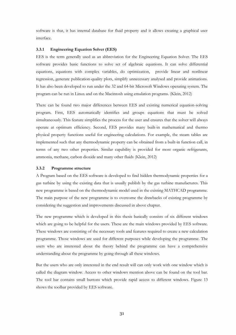
3.3.2 Programme structure

A Program based on the EES software is developed to find hidden thermodynamic properties for a

gas turbine by using the existing data that is usually publish by the gas turbine manufactures. This

new programme is based on the thermodynamic model used in the existing MATHCAD programme.

The main purpose of the new programme is to overcome the drawbacks of existing programme by

considering the suggestion and improvements discussed in above chapter.

The new programme which is developed in this thesis basically consists of six different windows

which are going to be helpful for the users. These are the main windows provided by EES software.

These windows are consisting of the necessary tools and features required to create a new calculation

programme. Those windows are used for different purposes while developing the programme. The

users who are interested about the theory behind the programme can have a comprehensive

understanding about the programme by going through all these windows.

But the users who are only interested in the end result will can only work with one window which is

called the diagram window. Access to other windows mention above can be found on the tool bar.

The tool bar contains small buttons which provide rapid access to different windows. Figure 13

shows the toolbar provided by EES software.

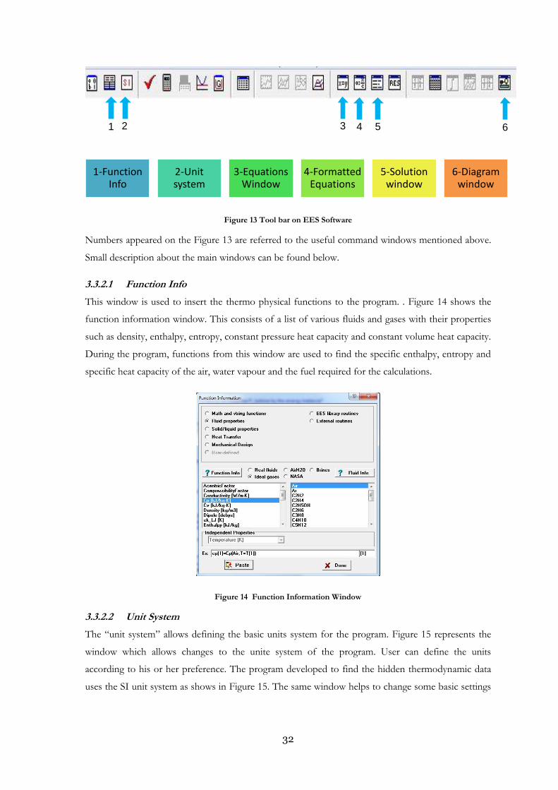
32

Figure 13 Tool bar on EES Software

Numbers appeared on the Figure 13 are referred to the useful command windows mentioned above.

Small description about the main windows can be found below.

3.3.2.1 Function Info

This window is used to insert the thermo physical functions to the program. . Figure 14 shows the

function information window. This consists of a list of various fluids and gases with their properties

such as density, enthalpy, entropy, constant pressure heat capacity and constant volume heat capacity.

During the program, functions from this window are used to find the specific enthalpy, entropy and

specific heat capacity of the air, water vapour and the fuel required for the calculations.

Figure 14 Function Information Window

3.3.2.2 Unit System

The “unit system” allows defining the basic units system for the program. Figure 15 represents the

window which allows changes to the unite system of the program. User can define the units

according to his or her preference. The program developed to find the hidden thermodynamic data

uses the SI unit system as shows in Figure 15. The same window helps to change some basic settings

1-Function Info

2-Unit system

3-Equations Window

4-Formatted Equations

5-Solution window

6-Diagram window

1 2 3 4 5 6

33

of the program such as display settings. These settings can be found by selecting the tabs shown

under the window.

Figure 15 Unit system Window

3.3.2.3 Equation window

This is the most important window for the program. Equation window is used to enter all

thermodynamic formulae and other related equations needed to be solved. EES allows the users to

enter the equations with unknown variables and it is not mandatory to rearrange the equation for the

variable to be solved. It is not needed to define the unknown variables in this program such as in

other software. EES will identify the unknown variables while running the program and will solve the

equations if there is enough number of equations to solve the unknowns.

There is a standard way to insert the equations to the equation window. EES software uses some

program cods to write equations in the equation window. The codes written in below can be

represented as an example for the way of writing the equations in equation window.

B=integral(((Cp(Air;T=T)+moisturecontent*Cp(H2O;T=T))/(T*(R_air+moisturecontent*R_H20)));T;Tin;T2)

3.3.2.4 Formatted Equations

Formatted window is an imported feature of EES software for the users. As explained above the

equations entered in the equation window are written using specific program codes. Formatted

window presents those equations in a graphical form with appropriate mathematical notations and

symbols. Figure 16 represents the formatted equation which is written above with program codes.

Figure 16: An example for a formatted equation

B = òT2

Tin

Cp ( 'Air' ; T =T ) + moisturecontent · Cp ( 'H2O' ; T =T )

T · ( Rair + moisturecontent · RH20 ) d T

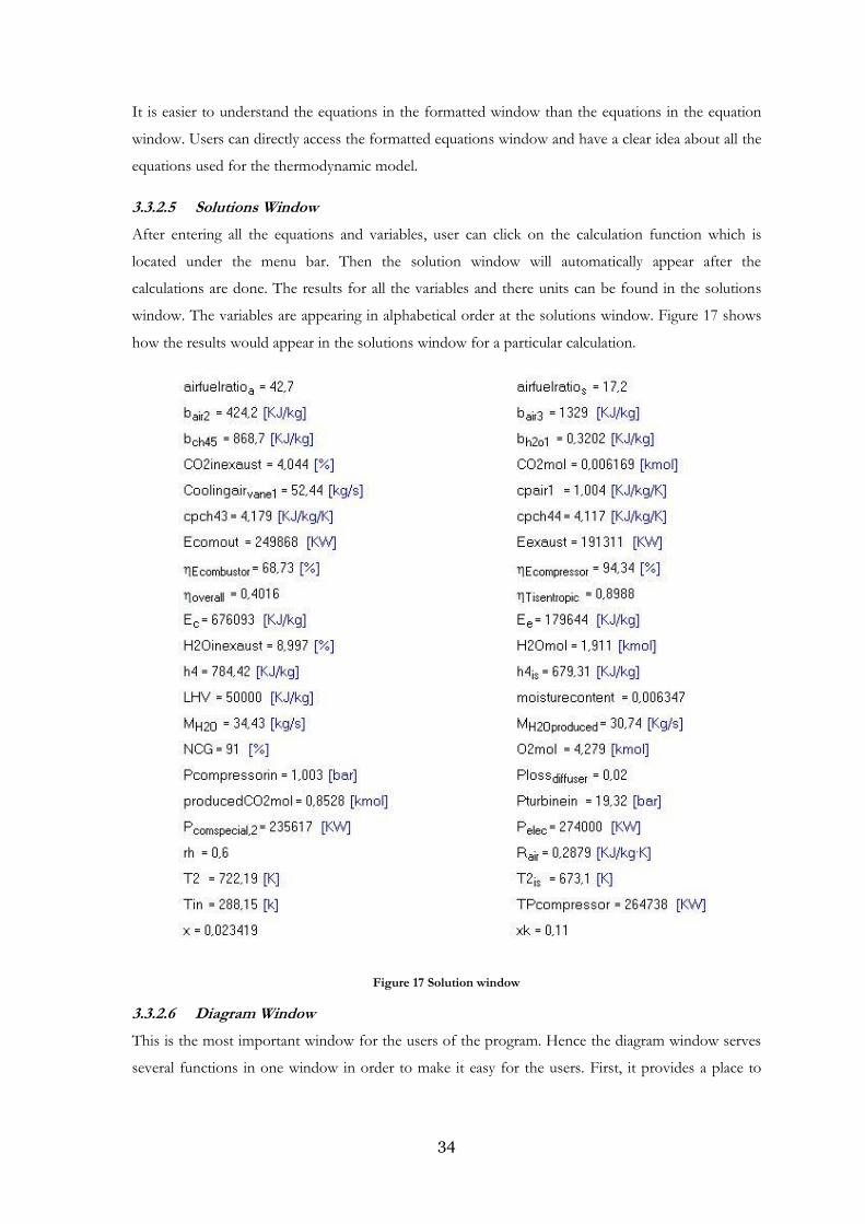
34

It is easier to understand the equations in the formatted window than the equations in the equation

window. Users can directly access the formatted equations window and have a clear idea about all the

equations used for the thermodynamic model.

3.3.2.5 Solutions Window

After entering all the equations and variables, user can click on the calculation function which is

located under the menu bar. Then the solution window will automatically appear after the

calculations are done. The results for all the variables and there units can be found in the solutions

window. The variables are appearing in alphabetical order at the solutions window. Figure 17 shows

how the results would appear in the solutions window for a particular calculation.

Figure 17 Solution window

3.3.2.6 Diagram Window

This is the most important window for the users of the program. Hence the diagram window serves

several functions in one window in order to make it easy for the users. First, it provides a place to

35

display graphics and text relating to the problem that is being solved. Users can observe and identify

the model for simple cycle gas turbine operation which is going to be used for the calculations.

Other than that the diagram window can be used to provide input data to the program and obtain the

results as outputs. Several functions are also added to the diagram window such as the calculate

button to run the program, the print button to print the results and a help button which allows to

open a help file or a website. Figure 18 shows the view of the diagram window of the new program.

Figure 18 Diagram window

3.3.3 Thermodynamic model

The new program based on EES software is also used to find the hidden thermodynamic parameters

by using available catalogue data publish by the manufacturer. To achieve this task a thermodynamic

model is defined for the gas turbine cycle. For that the same simple cycle gas turbine model which is

used in the Mathcad program is used for the new program. Figure 12 represent the thermodynamic

model used for the Mathcad program. The assumptions used for that model are also valid for the

new program. It also follows the same sequence of the flow as described under the Figure 12.

The model described in Figure 12 does not include the cooling air extraction lines used for the

cooling purposes of the turbine. Therefore, to analysis the effect from the cooling air extraction lines,

the above model is modified by adding two cooling air extraction lines form the compressor to the

turbine. Schematic diagram of the simple gas turbine cycle with cooling air extraction lines is shown

36

in Figure 19. The modified model is considered when finding the variables such as vane exit

temperature and the combustor exit temperature which are directly affected by the cooling air

extraction lines.

Figure 19 Model with cooling air extraction lines

3.3.3.1 Assumptions and simplifications

There are several assumptions and simplifications used while developing the programme. Some of

the assumptions were mentioned under chapter 3.1.1.2 which explains the thermodynamic model

used for the Mathcad programme.

1. Air, fuel and water contents in air are assumed as ideal gasses.

2. Constant pressure specific heat capacity ( ) is taken for the calculations.

3. All the thermodynamic properties were taken from the EES library.

4. It is assumed that the value of the specific heat capacity of flue gas is same as the value of

air-fuel mixture. This is valid for the fuels such as methane where the combustion process

happens without a volume change. Hence the flue gas mixture is replaced by air fuel mixture

for the energy calculations.

5. Flue gas analysis is done by considering the amount of moles of various gases in the flue gas.

Complete combustion of fuel in air is assumed for the calculations.

6. The temperature of the fuel is assumed to be at the ambient temperature.

3.3.4 Calculation procedure

Before understanding the calculation procedure, it is better to understand the input parameters to the

program. It will be useful to the users when they are working with the program. Mainly there are five

important input data which can be found in the turbine manufactures catalogue. The other input data

can be an assumption, standard or commonly available value in the field of gas turbine. Brief

37

description of each input parameters are given below. The variable name used in the EES program

also mention with the input parameter.

Electrical power output ( )

The electrical power output of the gas turbine is given in MW or KW. But the users should

input as KW to the programme. Sometimes the turbine manufacturers give the shaft power

of the turbine. At that time the shaft power can be added to the programme in KW with

putting the electrical efficiency (input data) as 1.

Plant overall efficiency ( )

The pant overall thermal efficiency can be added as an input data. The value for the thermal

efficiency should be in between 1 to 0.

Exhaust mass flow rate ( )

Exhaust mass flow rate of the power plant can be found in the turbine catalogue. Some

catalogues shows the mass flow rate in the unit of lb/sec while others give it as kg/sec. to

run the programme correctly this value should be entered in the unit of kg/sec. Sometimes

the turbine manufacturer gives the air inlet mass flow.so that the users must be careful about

that. The way of handling with inlet air mass flow rate discussed later.

Exhaust temperature of flue gas ( )

The exhaust temperature of the flue gas is given by the manufacturer and the value can be

found in the unit of 0C or 0F. For the programme the 0C value should be entered.

Pressure ratio of the compressor ( )

This represents the compressor pressure ratio and it is a given parameter in the gas turbine

catalogue. The most common definition of the pressure ratio is the ratio between

compressor exit plenum to ambient (Wettstein, 2006).

Inlet temperature ( )

This is the ambient temperature of the surrounding of the gas turbine. In ISO standards

conditions the value is equal to 288 K/ 15 0C. The units for the temperature values should

be in K (brighthubengineering, 2013).

38

Ambient pressure ( )

Pressure of the air at the air intake duct to the compressor named as the . In the

ISO standards the ambient pressure is 1.013 bars (brighthubengineering, 2013).

Relative humidity ( )

Relative humidity of the inlet air is also an input parameter. According to the standards value

for the relative humidity is 60% (brighthubengineering, 2013).

Compressor polytropic efficiency ( )

Compressor polytropic efficiency is the main assumption to the programme. Typical value

for axial compressor polytropic efficiency is in between 0.89 to 0.92 (Wettstein, 2006).

Electrical efficiency ( )

Electrical efficiency of the gas turbine can be varied with the gas turbine. It is depending on

the type of the electrical generator used in the gas turbine arrangement. If the value cannot

be found in the manufacture’s catalogue, realistic value for the can be used by the users

preference. Normally the electrical efficiency for an advanced air cooled generator is around

0.985 (Wettstein, 2006)

Mechanical efficiency ( )

Mechanical efficiency of the turbine also varies with the gas turbine arrangement. If the

turbine directly coupled to the generator, mechanical efficiency of the system is higher or if

there is a gear arrangement in between the turbine and generator, there can be 3% to 4%

mechanical energy loss (Wettstein, 2006). Because of that the user can choose suitable

value accordingly.

Relative inlet pressure loss ( )

This value refers the pressure loss occurred from ambient to compressor inlet. This pressure

loss occurs due to the presence of air filters to clean the inlet air. 0.004 is a typical value for

relative inlet pressure loss for a compressor with standard air filters. (Wettstein, 2006). If the

user can find better data for this value it can be used instead the typical value

above.

Compressor relative diffuser loss ( )

39

The compressor relative diffuser loss refers the pressure loss occurring at the diffuser or the

exit of the compressor. This value also depending upon the gas turbine and hence user can

use more realistic value for the . 0.02 is a realistic assumption for the

compressor relative diffuser loss.

Relative intermediate pressure loss ( )

The relative intermediate pressure loss represents the pressure loss occurring from

compressor exit to the turbine inlet. The values for can be found in the

order of 0.05 to 0.08 (Wettstein, 2006).

Relative outlet pressure loss( )

Relative outlet pressure loss indicates the pressure loss happens from turbine outlet to the

exit of the stack. The typical value for the outlet pressure loss is 0.013. This value is going to

change with the arrangement of the gas turbine. Presence of HRSG unit in the downstream

of the flue gas can increase the pressure loss up to 0.043 (Wettstein, 2006).

Lower heating value ( )

Lower heating value of the fuel used in the gas turbine should be entered to the programme.

The units should be KJ/Kg. Depending on the fuel the value going to be change. The value

can be found in the standard books or tables.

Chemical exergy ( )

Chemical exergy of the fuel is also an input parameter. The value for chemical exergy of the

fuel can found in the standard books.

Other than the above input parameters another two input data can be found in the programme. They

are related to cooling air extraction lines. These values should be given by the manufacture or the

user should know the values by his experience and knowledge. If the user does not know the real

value he can put zero by assuming there are no cooling air extraction lines. Then the programme

solves the unknowns or the hidden thermodynamic parameters by considering the all the air mass

flow rate leaving the compressor is going through the combustion chamber.

40

Cooling air ratio vane 1 ( )

This is the percentage of cooling air extraction mass flow rate to the first vane of the turbine.

The value is given as a percentage to inlet dry air mass flow rate. This value should be given

by the manufacture or the user must know. If the user does not know the value it is better to

put the value as zero.

Cooling air ratio downstream of vane 1 ( )

The value for cooling air ratio downstream of vane 1 represents the cooling air mass flow

rate to the turbine components after the first set of vanes. This value also should be given by

the manufacture or the user must know. If the user does not know the value it is better to

put the value as zero.

When a user wants to run the programme the first step is to insert the input data to the programme.

Graphical user interface of the EES programme which is displayed in the diagram window is used to

insert the input parameters to the program. User can find all the input parameters discussed above on

that diagram window. The input section is divided in to three sub sections. They were listed below.

1. Given data by the manufactures.

The main five input parameters given by the manufacturer can be entered here.

2. Related input data.

The other input data related to the calculations can be found here.

3. Assumption.

Compressor polythropic efficiency is the main assumption to the programme. That

value can be added here.

Figure 20 shows the figure of three different input sections appears in the diagram window. Users

can enter the values for the input variables by clicking on the boxes which appear in front of the

variable name.

41

Figure 20 Input section of the programme

After entering all the input data accordingly user can run the programme. There is a button which

name as “Calculate “can be found in the diagram window. User can click that button also shows in

Figure 21, to start the calculation process.

Figure 21 calculate button in the programme

After clicking that button the programme is started to run. Then suddenly there is a pop-up window

appearing on the screen. If there are no errors with the input data such as the mistakes of comma or

dot for the decimal point it takes several seconds to finish the calculations process. When the

calculation is done the pop-up window appear with a “Continue” button as in Figure 22.

Figure 22 popup window

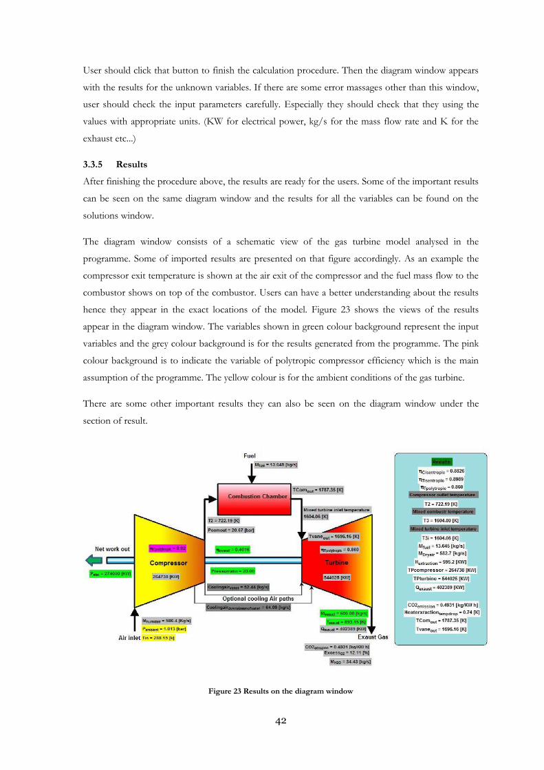
42

User should click that button to finish the calculation procedure. Then the diagram window appears

with the results for the unknown variables. If there are some error massages other than this window,

user should check the input parameters carefully. Especially they should check that they using the

values with appropriate units. (KW for electrical power, kg/s for the mass flow rate and K for the

exhaust etc...)

3.3.5 Results

After finishing the procedure above, the results are ready for the users. Some of the important results

can be seen on the same diagram window and the results for all the variables can be found on the

solutions window.

The diagram window consists of a schematic view of the gas turbine model analysed in the

programme. Some of imported results are presented on that figure accordingly. As an example the

compressor exit temperature is shown at the air exit of the compressor and the fuel mass flow to the

combustor shows on top of the combustor. Users can have a better understanding about the results

hence they appear in the exact locations of the model. Figure 23 shows the views of the results

appear in the diagram window. The variables shown in green colour background represent the input

variables and the grey colour background is for the results generated from the programme. The pink

colour background is to indicate the variable of polytropic compressor efficiency which is the main

assumption of the programme. The yellow colour is for the ambient conditions of the gas turbine.

There are some other important results they can also be seen on the diagram window under the

section of result.

Figure 23 Results on the diagram window

43

A brief description about some of the important results or variables can be found below. The

variable used in the EES programme also mention within the brackets.

Inlet air mass flow rate( )

This represents the total mass flow rate of air to the compressor. It includes the mass flow

rate of dry air and the water content of the incoming air.

Compressor outlet pressure( )

Compressor outlet pressure is indicated from this variable.

Mixed combustor temperature ( )

Mixed combustor temperature represents the temperature of the flue gas at the combustion

chamber outlet provided that the entire air flow at the compressor inlet enters the

combustion chamber. This is the definition according to the ISO 2314 (1989) (Wettstein,

2006).

Mixed turbine inlet temperature ( )

Mixed turbine inlet temperature represents the temperature of the flue gas at the turbine inlet

provided that the entire air flow at the compressor inlet enters the combustion chamber

(Wettstein, 2006).

44

Combustor outlet temperature ( )

This is the real flue gas temperature at the combustor exit. For the calculation of combustor

outlet temperature, cooling air extraction lines are taken into consideration. Hence the air

mass flow rate through the combustion chamber is less than the mass flow rate of air at the

compressor inlet and the value for combustion outlet temperature is higher than the mixed

combustor temperature.

Vane exit temperature ( )

Vane exit temperature is the temperature of the flue gas at the first vane of the turbine. At

the first vane of the turbine the flue gas from the combustor is mixed with the cooling air

mass flow to the vane one.

Heat extraction temperature drop ( )

Some of the gas turbines consist of external cooling air lines or steam cooling lines. These

cooling lines are placed in between the combustor and the turbine to protect the

components from high temperatures. Due to this cooling lines heat extraction can happen

(Wettstein, 2007). If there is a heat extraction there is also a temperature drop of the flue gas

due to the heat extraction. Heat extraction temperature drop shows the temperature

difference between mixed combustor temperature and the mixed turbine inlet temperature.

Heat extraction ( )

This indicates the amount of heat extracted from the gas turbine due to the presence of

external cooling lines. Even though there are no any external cooling lines it can have a small

heat loss to the surroundings.

Energy content of the exhaust( )

The heat energy content of the flue gas is given by this parameter.

Including above there are several important variables that can be seen on the diagram window. If the

users are interested on the results for all the variables, they can find all the results in the solution

window. Some of the variables are listed in Table 4 with the results generated by the EES

programme. The given input variables are exactly as same as the data given in Table 3 which are used

to run the Mathcad programme.

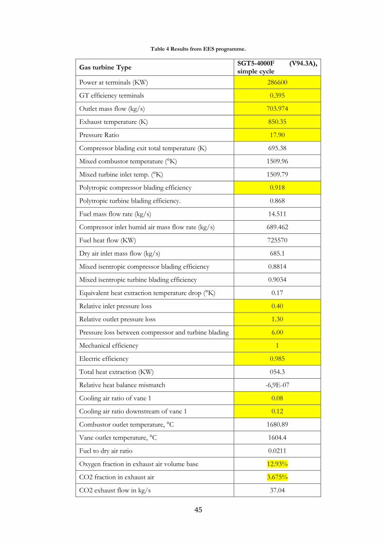
45

Table 4 Results from EES programme.

Gas turbine Type SGT5-4000F (V94.3A), simple cycle

Power at terminals (KW) 286600

GT efficiency terminals 0.395

Outlet mass flow (kg/s) 703.974

Exhaust temperature (K) 850.35

Pressure Ratio 17.90

Compressor blading exit total temperature (K) 695.38

Mixed combustor temperature (°K) 1509.96

Mixed turbine inlet temp. (°K) 1509.79

Polytropic compressor blading efficiency 0.918

Polytropic turbine blading efficiency. 0.868

Fuel mass flow rate (kg/s) 14.511

Compressor inlet humid air mass flow rate (kg/s) 689.462

Fuel heat flow (KW) 725570

Dry air inlet mass flow (kg/s) 685.1

Mixed isentropic compressor blading efficiency 0.8814

Mixed isentropic turbine blading efficiency 0.9034

Equivalent heat extraction temperature drop (°K) 0.17

Relative inlet pressure loss 0.40

Relative outlet pressure loss 1.30

Pressure loss between compressor and turbine blading 6.00

Mechanical efficiency 1

Electric efficiency 0.985

Total heat extraction (KW) 054.3

Relative heat balance mismatch -6,9E-07

Cooling air ratio of vane 1 0.08

Cooling air ratio downstream of vane 1 0.12

Combustor outlet temperature, °C 1680.89

Vane outlet temperature, °C 1604.4

Fuel to dry air ratio 0.0211

Oxygen fraction in exhaust air volume base 12.93%

CO2 fraction in exhaust air 3.675%

CO2 exhaust flow in kg/s 37.04

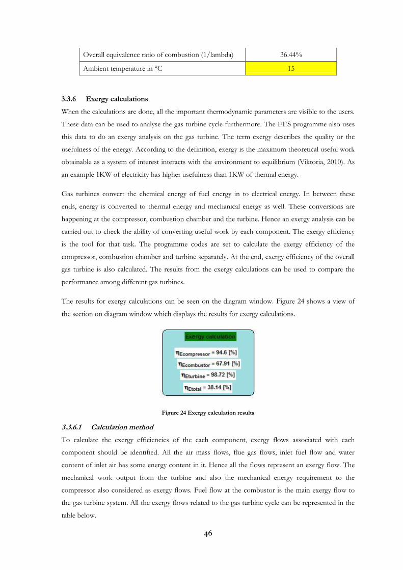
46

Overall equivalence ratio of combustion (1/lambda) 36.44%

Ambient temperature in °C 15

3.3.6 Exergy calculations

When the calculations are done, all the important thermodynamic parameters are visible to the users.

These data can be used to analyse the gas turbine cycle furthermore. The EES programme also uses

this data to do an exergy analysis on the gas turbine. The term exergy describes the quality or the

usefulness of the energy. According to the definition, exergy is the maximum theoretical useful work

obtainable as a system of interest interacts with the environment to equilibrium (Viktoria, 2010). As

an example 1KW of electricity has higher usefulness than 1KW of thermal energy.

Gas turbines convert the chemical energy of fuel energy in to electrical energy. In between these

ends, energy is converted to thermal energy and mechanical energy as well. These conversions are

happening at the compressor, combustion chamber and the turbine. Hence an exergy analysis can be

carried out to check the ability of converting useful work by each component. The exergy efficiency

is the tool for that task. The programme codes are set to calculate the exergy efficiency of the

compressor, combustion chamber and turbine separately. At the end, exergy efficiency of the overall

gas turbine is also calculated. The results from the exergy calculations can be used to compare the

performance among different gas turbines.

The results for exergy calculations can be seen on the diagram window. Figure 24 shows a view of

the section on diagram window which displays the results for exergy calculations.

Figure 24 Exergy calculation results

3.3.6.1 Calculation method

To calculate the exergy efficiencies of the each component, exergy flows associated with each

component should be identified. All the air mass flows, flue gas flows, inlet fuel flow and water

content of inlet air has some energy content in it. Hence all the flows represent an exergy flow. The

mechanical work output from the turbine and also the mechanical energy requirement to the

compressor also considered as exergy flows. Fuel flow at the combustor is the main exergy flow to

the gas turbine system. All the exergy flows related to the gas turbine cycle can be represented in the

table below.

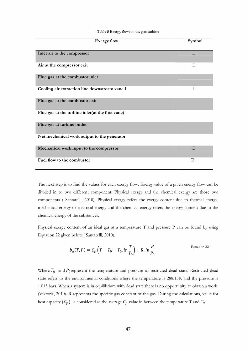
47

Table 5 Exergy flows in the gas turbine

Exergy flow Symbol

Inlet air to the compressor

Air at the compressor exit

Flue gas at the combustor inlet

Cooling air extraction line downstream vane 1

Flue gas at the combustor exit

Flue gas at the turbine inlet(at the first vane)

Flue gas at turbine outlet

Net mechanical work output to the generator

Mechanical work input to the compressor

Fuel flow to the combustor

The next step is to find the values for each exergy flow. Exergy value of a given energy flow can be

divided in to two different component. Physical exergy and the chemical exergy are those two

components ( Santarelli, 2010). Physical exergy refers the exergy content due to thermal energy,

mechanical energy or electrical energy and the chemical energy refers the exergy content due to the

chemical energy of the substances.

Physical exergy content of an ideal gas at a temperature T and pressure P can be found by using

Equation 22 given below ( Santarelli, 2010).

( ) (

)

Equation 22

Where and represent the temperature and pressure of restricted dead state. Restricted dead

state refers to the environmental conditions where the temperature is 288.15K and the pressure is

1.013 bars. When a system is in equilibrium with dead state there is no opportunity to obtain a work.

(Viktoria, 2010). R represents the specific gas constant of the gas. During the calculations, value for

heat capacity ( ) is considered as the average value in between the temperature T and T0.

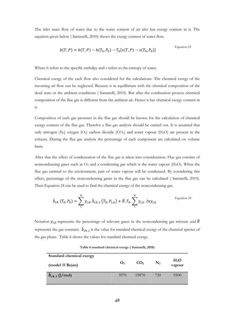
48

The inlet mass flow of water due to the water content of air also has exergy content in it. The

equation given below ( Santarelli, 2010) shows the exergy content of water flow.

( ) ( ) ( ) [ ( ) ( )]

Equation 23

Where h refers to the specific enthalpy and s refers to the entropy of water.

Chemical exergy of the each flow also considered for the calculations. The chemical exergy of the

incoming air flow can be neglected. Because it in equilibrium with the chemical composition of the

dead state or the ambient conditions ( Santarelli, 2010). But after the combustion process chemical

composition of the flue gas is different from the ambient air. Hence it has chemical exergy content in

it.

Composition of each gas presennt in the flue gas should be known for the calculation of chemical

exergy content of the flue gas. Therefor a flue gas analysis should be carried out. It is assumed that

only nitrogen (N2) oxygen (O2) carbon dioxide (CO2) and water vapour (H2O) are present in the

exhaust. During the flue gas analysis the percentage of each component are calculated on volume

basis.

After that the effect of condensation of the flue gas is taken into consideration. Flue gas consists of

noncondensing gases such as O2 and a condensing gas which is the water vapour (H2O). When the

flue gas emitted to the environment, part of water vapour will be condensed. By considering this

effect, percentage of the noncondensing gases in the flue gas can be calculated ( Santarelli, 2010).

Then Equation 24 can be used to find the chemical exergy of the noncondensing gas.

( ) ∑

( ) ∑

Equation 24

Notation represents the percentage of relevant gases in the noncondensing gas mixture and

represents the gas constant. is the value for standard chemical exergy of the chemical species of

the gas phase. Table 6 shows the values for standard chemical exergy.

Table 6 standard chemical exergy ( Santarelli, 2010)

Standard chemical exergy

(model 11 Bejan) O2 CO2 N2

H2O vapour

(J/mol) 3970 19870 720 9500

49

Part of the condensing gas or the water vapour will make liquid water when the flue gas gets cooled

down. That liquid water also has chemical exergy content on it. Considering the standard chemical

exergy of the liquid water phase the value is 900 (J/mol) ( Santarelli, 2010).

By considering both chemical exergy of the gas and condensation water, chemical exergy of the flue

gas can be calculated. Then the exergy flows of air and flue gas can be calculated. Chemical exergy of

the fuel also be found out from standard Tables.

Next step is to define the exergy efficiency for each component. As mentioned above there are three

main components in the gas turbine cycle. Each component has a fuel exergy to and a product

exergy. The exergy flow supplied to the component is called as the fuel and the product is the change

of exergy flow or the exergy output by the component. The ratio between the product and the fuel

can be given as the exergy efficiency of the component.

Compressor uses mechanical energy to increase the exergy of incoming air. The fuel for the

compressor is mechanical work. According to the exergy definition mechanical work can be

considered as pure exergy (Viktoria, 2010). The product is the increase of exergy in the air flow. Then

the exergy efficiency of the compressor can be given in the Equation 25 ( Santarelli, 2010).

Equation 25

The next component is the combustion chamber. It uses the chemical exergy content of the fuel flow

in order to increase the specific exergy content of the air entering to the combustion chamber.

Equation 26 gives the exergy efficiency for the combustion chamber.

Equation 26

There are two main exergy flows entering the turbine. First exergy flow is the flue gas at turbine inlet.

This is mixed with a fraction of the cooling air at vane 1. Both streams are mixed at the vane and

hence it is assumed as one flow. And the second exergy flow is the cooling air flow after vane one.

Both streams leave the turbine at the turbine exit as one stream. Turbine uses the above exergy flows

to produce the net mechanical work output to the generator and mechanical power requirement by

the compressor ( Santarelli, 2010). The equation below will give the exergy efficiency of the turbine.

Equation 27

At the end, overall exergy efficiency of the gas turbine cycle can be calculated. The exergy flow to the

overall gas turbine system is the fuel exergy from the fuel and the product is the net mechanical

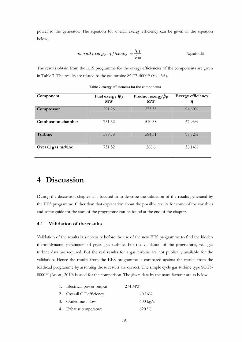
50

power to the generator. The equation for overall exergy efficiency can be given in the equation

below.

Equation 28

The results obtain from the EES programme for the exergy efficiencies of the components are given

in Table 7. The results are related to the gas turbine SGT5-4000F (V94.3A).

Table 7 exergy efficiencies for the components

Component Fuel exergy MW

Product exergy MW

Exergy efficiency

Compressor 291.26 275.53 94.60%

Combustion chamber 751.52 510.38 67.93%

Turbine 589.78 584.31 98.72%

Overall gas turbine 751.52 288.6 38.14%

4 Discussion

During the discussion chapter it is focused in to describe the validation of the results generated by

the EES programme. Other than that explanation about the possible results for some of the variables

and some guide for the uses of the programme can be found at the end of the chapter.

4.1 Validation of the results

Validation of the results is a necessity before the use of the new EES programme to find the hidden

thermodynamic parameters of given gas turbine. For the validation of the programme, real gas

turbine data are required. But the real results for a gas turbine are not publically available for the

validation. Hence the results from the EES programme is compared against the results from the

Mathcad programme by assuming those results are correct. The simple cycle gas turbine type SGT6-

8000H (Anon., 2010) is used for the comparison. The given data by the manufacturer are as below.

1. Electrical power output 274 MW

2. Overall GT efficiency 40.16%

3. Outlet mass flow 600 kg/s

4. Exhaust temperature 620 °C

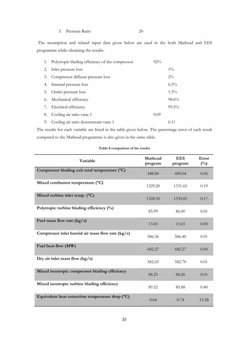
51

5. Pressure Ratio 20

The assumption and related input data given below are used in the both Mathcad and EES

programme while obtaining the results.

1. Polytropic blading efficiency of the compressor 92%

2. Inlet pressure loss 1%

3. Compressor diffuser pressure loss 2%

4. Internal pressure loss 6.5%

5. Outlet pressure loss 1.3%

6. Mechanical efficiency 98.6%

7. Electrical efficiency 99.5%

8. Cooling air ratio vane 1 0.09

9. Cooling air ratio downstream vane 1 0.11

The results for each variable are listed in the table given below. The percentage error of each result

compared to the Mathcad programme is also given in the same table.

Table 8 comparison of the results

Variable Mathcad program

EES program

Error (%)

Compressor blading exit total temperature (°C) 448.80 449.04 0.06

Mixed combustor temperature (°C) 1329.20 1331.65 0.19

Mixed turbine inlet temp. (°C) 1328.50 1330.85 0.17

Polytropic turbine blading efficiency (%) 85.99 86.00 0.01

Fuel mass flow rate (kg/s) 13.65 13.65 0.00

Compressor inlet humid air mass flow rate (kg/s) 586.36 586.40 0.01

Fuel heat flow (MW) 682.27 682.27 0.00

Dry air inlet mass flow (kg/s) 582.65 582.70 0.01

Mixed isentropic compressor blading efficiency 88.25 88.26 0.01

Mixed isentropic turbine blading efficiency 89.52 89.88 0.40

Equivalent heat extraction temperature drop (°C) 0.64 0.74 15.28

52

Total heat extraction (MW) 0.52 0.59 13.28

Relative heat balance mismatch 9.1 E-07 7.1 E-08 -92.20

Combustor outlet temperature, °C 1509.30 1514.20 0.33

Vane outlet temperature, °C 1419.50 1423.01 0.25

Fuel to dry air ratio (%) 2.34 2.34 0.00

The table shows that the deviations of the results from the benchmark figures are less than 0.5%.

However there are three exceptions. Those are total heat extraction, relative heat balance mismatch

and the heat extraction temperature drop. The values for these three variables are extremely small

compared to the other variables. Relative heat balance mismatch is in the order of minus seven (9.1E-

07),and the heat extraction temperature drop is less than 1 K, and the total heat extraction is only

0.59 MW which is negligible compared to the electrical power output (274 MW).

4.1.1 Effect of heat capacity ( ) on the temperature results

At the outset it can be seen that the percentage error for the temperature values increase with the

increase of the temperature. Table 9 shows all the variables representing the temperature values from

the programme. These variables are listed in the ascending order of the temperature vales.

Table 9 Temperature results

Variable Mathcad program

EES program

Error (%)

Compressor blading exit total temperature (°C) 448.80 449.04 0.06

Mixed turbine inlet temp. (°C) 1328.50 1330.85 0.17

Mixed combustor temperature (°C) 1329.20 1331.65 0.19

Vane outlet temperature, °C 1419.50 1423.01 0.25

Combustor outlet temperature, °C 1509.30 1514.20 0.33

The reason for this pattern has been revealed through a deep thermodynamic analysis. An error in

temperature can be the cause for the errors in the other variables as a thermodynamic system all the

parameters are influenced by the temperature. These temperature values are obtained mostly by

53

solving the thermodynamic equations most of which are dependent on the heat capacity ( ) of air.

Therefore it is predicted that the reason behind the temperature variation is the difference of heat

capacity ( ) value between both programs. It can be a possible prediction because the Mathcad

programme uses a different property library than the property libraries in the EES programme.

Hence to observe the difference of heat capacities between the two programs the variation of is

plotted against the temperature. Figure 25 shows the variation of for both Mathcad and EES

programs.

By observing the Figure 25 it can be seen that there is a difference between the values of dry air

used by the both programs. According to the figure value used by the Mathcad programme are

higher than the value used by the EES programme. The figure also shows that the difference of

value is increased with the temperature.

Figure 25 variation of Cp between the Mathcad and EES

The percentage of temperature difference given in the Table 9 and also the difference of value in

both programmes are increased with the temperature. Hence it can be shown that the error is

occurred due to the variation of .

Furthermore there is another argument which can prove the effect of . The temperature results are

obtained from EES programme are always higher than the results from Mathcad programme and the

value of EES programme is always lower than the Mathcad programme. There is a reason behind

that. Both programmes handle same amount of energy and an energy value represents a

0,9

0,95

1

1,05

1,1

1,15

1,2

1,25

1,3

1,35

1,4

1,45

1,5

0 200 400 600 800 1000 1200 1400 1600 1800 2000 2200

Cp

(K

J/kg

)

Temperature (K)

Cp of Dry air (EES vs Mathcad)

EES

MathCad

54

multiplication of temperature difference into heat capacity ( ) . To have same energy content in

particular components or streams, EES programme calculations should give higher temperature

differences because it has lower values.

By considering above arguments it can be verified that the temperature difference occurred in

between the Mathcad and EES programs is due to the difference of .So that the results that are

generated from the EES programme could have even smaller variations (smaller than 0.5%) from the

Mathcad programme. The differences of values for fuel and water vapour in air could have

imposed a similar effect on the validation process nevertheless such effects were not analysed due to

the very small mass flow rates compared to air mass flow rate.

4.1.2 Effect of heat capacity ( ) on the exergy calculations

Exergy calculations on gas turbine components are also included in the new EES program. The

exergy efficiency of the compressor, combustion chamber and the overall gas turbine was calculated.

Exergy calculations for a gas turbine have more value when used for the comparison of gas turbines.

Then the exergy efficiency of each component can be compared to each other separately.

The results obtained for the exergy efficiency of the compressor and turbine show high values.

Especially the exergy efficiency of the turbine has a value around 98%. But in practise it seems that

these values are little bit higher. The exergy calculations however are directly affected by the Cp value

as the equation which used to find the physical exergy (Equation 22) contains a heat capacity

component. Therefore an average cp value between the stream temperature (T) and dead state

temperature (T0) is taken.

To see the effect of , the program was rearranged with the value that corresponds to the

temperature of the stream (T) instead of the average value. Then the result for the exergy

efficiency of the turbine was around 87%. This is a considerable deviation from the previous result

which is 98%. It clearly shows that there is huge effect of on the exergy calculation. Hence the

programme uses the average value in the physical exergy equation.

4.2 Possible running errors and rectification measures

The main important step to generate acceptable results is that the input data should be entered

properly and accordingly. The proper way of entering the input data was already discussed in the

chapter “calculation procedure”. As clarified in the same chapter, if there were no mistakes such as

wrong use of coma or dot for decimal point the programme will run and deliver the results.

By looking at some of the results, further analysis can be done to verify the accuracy of the

calculations. Heat extraction temperature drop is one of the main variables that can be used for this

55

analysis. For the gas turbines which do not have external air or steam cooling lines, heat extraction

temperature drop should be approximately less than 1 K. If there is no any heat extraction in

between the combustion chamber and the turbine inlet the heat extraction temperature drop should

be minimal. But the results shouldn’t be less than zero.

After the results generation, users can check the value for the “heat extraction temperature drop”. If

the value is less than zero, input variables have some error. Main possible errors can be the exhaust

mass flow rate, electrical efficiency and mechanical efficiency. If the “heat extraction temperature

drop” value is considerably high value it can be due to two reasons. First one is that the turbine has

an external cooling system. Presence of external cooling lines creates the heat extraction and hence

creates a “heat extraction temperature drop”. If there is no error with the input values user can

predict that the gas turbine has an external cooling system. The result for heat extraction also gives

the same indication.

The heat extraction temperature drop can also be higher due to less exhaust air mass flow rate than

the actual value. This situation can happen when the user inserts the exhaust mass flow rate

inaccurately. Some manufactures publish the air inlet mass flow rate instead of the exhaust mass flow

rate in their catalogues. During such situations users can misunderstand the inlet mass flow rate as

the exhaust mass flow rate.But the programme does not give the freedom to the users to insert inlet

air mass flow rate as the exhaust mas flow rate. Users can overcome this situation by following the

procedure explained below.

Exhaust mass flow rate is the summation of inlet air mass flow rate and the inlet fuel flow rate. If the

users can find the inlet fuel flow rate they can predict the exhaust flow rate. So that the users can run

the programme by feeding the given mass flow rate and obtained the results for the inlet fuel flow

rate. According to the thermodynamic model and the formulae, fuel flow rate is not dependant on

the mass flow rate but on the electrical power output and the overall efficiency of the plant. Hence

the value for the fuel flow rate can be accepted.

Then the user can take the summation of inlet fuel flow rate found out by the program and the inlet

air flow rate by the manufacturer and insert as the exhaust mass flow rate. Then the programme can

be run with the corrected mass flow rate. The new results can be considered as accurate predictions

for the hidden thermodynamic variables.

Another similar mistake can be observed with the electrical power output. Some of the

manufacturers publish the shaft power of the turbine instead of the electrical power output. To

overcome the situation shaft power can be fed in to the programme with the electrical efficiency as

100%.

56

5 Conclusions

In this thesis work, the new EES program is developed by introducing improvements and additional

features to the existing Mathcad programme to find out the hidden performance data for a gas

turbine. Furthermore, the task has been achieved in accordance with the set of objectives defined in

the beginning of this report.

One of the main objectives was to develop a graphical user interface to improve the user friendliness.

Hence, the insertion of input data, running the programme, and observation of results can now be

done on the same graphical interface in a single window.

The existing programme is limited to the analysis of gas turbines that only use methane as the fuel.

New EES program can easily be modified to run other gaseous fuels as well. The availability of the

thermodynamic properties for a number of liquid and gaseous fuels is a main advantage for the new

EES programme. Also the Mathcad programme uses only certain external libraries to find out

required thermodynamic properties. In contrast the new EES program has inbuilt libraries to recall

fuel properties which reduces the complexity of the program by a great deal. And also the users can

modify the new EES program for different fuels because of the availability of thermodynamic

properties for several fuels. The EES program already runs with the fuel as ethane and obtained

results. Results are not yet validated, because of unavailability of the real results.

The new EES program has a higher analytical capacity than the existing Mathcad programme. A

complete flue gas analysis is carried out by the new program. Exergy calculation for each component

of the gas turbine is a newly introduced feature. The users can use exergy values for the comparison

of different gas turbine components and also for the comparison of different gas turbines as a whole.

The new program contains a step by step elaboration of the calculation process. Hence it improves

the comprehensibleness for the users. The pedagogical users can easily go through all the calculation

steps and can have a better understanding about the program. It also helps to make the program

readily adoptable into education platforms such as CompEdu.

The users are given the freedom to change the program according to their preferences. They can re-

arrange the thermodynamic model and equations to achieve their educational goals. The step by step

elaboration and explanations will help them to understand the program very well and do their

changes conveniently. Thereby, students can enhance their knowledge about the gas turbine by

working with this programme model. Other than that this programme can readily be used in the

industrial capacity for the comparison of gas turbines performances.

57

6 Bibliography

Rahman, M. M., Ibrahim, T. K. & Abdalla, A. N., 2011. Thermodynamic performance

analysis of gas-turbine. Volume 6.

Santarelli, M., 2010. Exergy Analysis on Applications in CHP. s.l.:s.n.

Anon., 2010. handbook, Gas turbine world 2010 GTW, s.l.: pequot Publication.

Anon., 2013. Gas Turbine Jet Engine Theory. [Online]

Available at: http://www.chrisbence.com/projects/gasturbine/gasturbine1.htm

[Accessed 23 04 2013].

Biasi, V. d., 2005. Catalog performance data can reveal hidden design features. Gas

Turbine World.

brighthubengineering, 2013. What is ISO rating of Gas Turbines. [Online]

Available at: http://www.brighthubengineering.com/power-plants/25425-what-is-iso-

rating-of-gas-turbines/

Brooks, F. J., 2005. GE Gas Turbine performance Charactristics, GE Power Systems

Schenecady;NY: s.n.

Cengel, Y. A. & Boles, M. A., 2006. Thermodynamics An Engineering Approach. s.l.:s.n.

compedu, 2013. [Online]

Available at: http://www.compedu.net/

Energy and environmantal analysis (an icf international company), 2008. Technology

charracterization:gas Turbines. Virginia: s.n.

Gandiglio M, et al., n.d. Thermoeconomic analysis of large solid oxide fuel cell plants:

atmospheric vs. pressurized performance. s.l., s.n.

Jan, s., Antonio, V., Wojciech, S. & Alicia, V., 2013. Towards an international Reference

Environment of Chemical Exergy. Zaragoza,Spain, s.n.

Klein, S., 2012. EES Engineering Equation Solver for Microsoft Operating Systems, s.l.:

s.n.

MathSoft, I., 2000. Mathcad User`s Guide, Massachusett: s.n.

58

Saravanamutto, H., Rogers, G. & Cohen, H., 2001. Gas Turbine Theory. s.l.:s.n.

Wettstein, H. E., 2006. CompEdu Chapter, s.l.: KTH.

Wettstein, H. E., 2007. Lecture on gas turbine cycle analysis aimed at application to

catalog data. ASME Turbo Expo 2007:.

wikipedia, 2013. [Online]

Available at: http://en.wikipedia.org/wiki/Density_of_air

Viktoria, M., 2010. The Exergy Concept – Physical Exergy. s.l.:s.n.

Wylen, G. V. & Sonntag, R., 1976. Fundamental of classical thermodynamics. New York:

John Wiley & Sons.

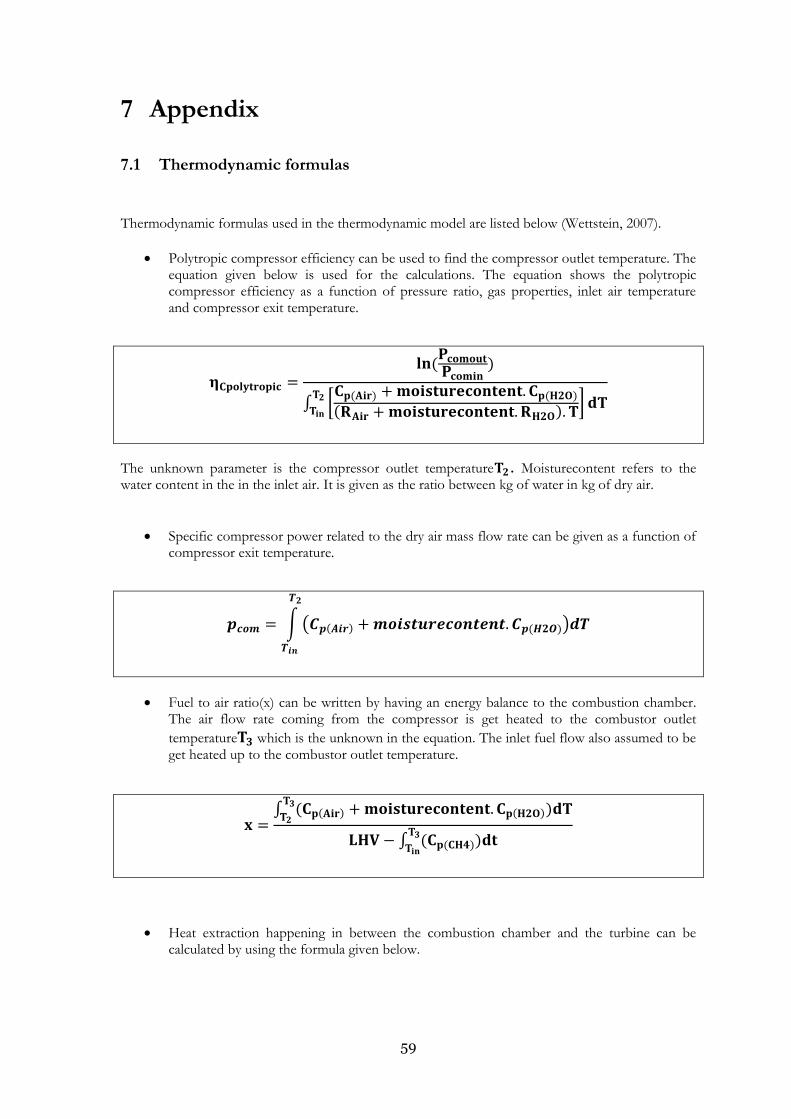
59

7 Appendix

7.1 Thermodynamic formulas

Thermodynamic formulas used in the thermodynamic model are listed below (Wettstein, 2007).

Polytropic compressor efficiency can be used to find the compressor outlet temperature. The equation given below is used for the calculations. The equation shows the polytropic compressor efficiency as a function of pressure ratio, gas properties, inlet air temperature and compressor exit temperature.

(

)

∫ [ ( ) ( )( )

]

The unknown parameter is the compressor outlet temperature . Moisturecontent refers to the water content in the in the inlet air. It is given as the ratio between kg of water in kg of dry air.

Specific compressor power related to the dry air mass flow rate can be given as a function of compressor exit temperature.

∫ ( ( ) ( ))

Fuel to air ratio(x) can be written by having an energy balance to the combustion chamber. The air flow rate coming from the compressor is get heated to the combustor outlet

temperature which is the unknown in the equation. The inlet fuel flow also assumed to be get heated up to the combustor outlet temperature.

∫ ( ( ) ( ))

∫ ( ( ))

Heat extraction happening in between the combustion chamber and the turbine can be calculated by using the formula given below.

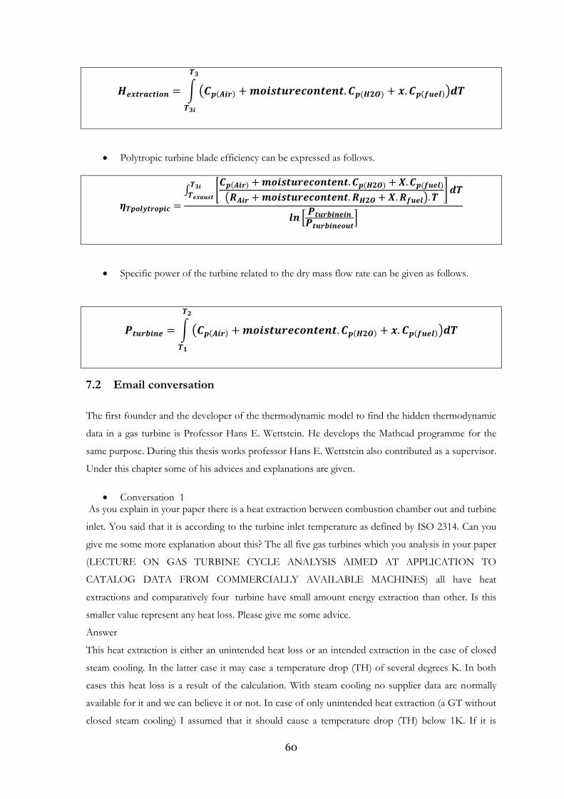
60

∫ ( ( ) ( ) ( ))

Polytropic turbine blade efficiency can be expressed as follows.

∫ [ ( ) ( ) ( )( )

]

[

]

Specific power of the turbine related to the dry mass flow rate can be given as follows.

∫ ( ( ) ( ) ( ))

7.2 Email conversation

The first founder and the developer of the thermodynamic model to find the hidden thermodynamic

data in a gas turbine is Professor Hans E. Wettstein. He develops the Mathcad programme for the

same purpose. During this thesis works professor Hans E. Wettstein also contributed as a supervisor.

Under this chapter some of his advices and explanations are given.

Conversation 1 As you explain in your paper there is a heat extraction between combustion chamber out and turbine

inlet. You said that it is according to the turbine inlet temperature as defined by ISO 2314. Can you

give me some more explanation about this? The all five gas turbines which you analysis in your paper

(LECTURE ON GAS TURBINE CYCLE ANALYSIS AIMED AT APPLICATION TO

CATALOG DATA FROM COMMERCIALLY AVAILABLE MACHINES) all have heat

extractions and comparatively four turbine have small amount energy extraction than other. Is this

smaller value represent any heat loss. Please give me some advice.

Answer

This heat extraction is either an unintended heat loss or an intended extraction in the case of closed

steam cooling. In the latter case it may case a temperature drop (TH) of several degrees K. In both

cases this heat loss is a result of the calculation. With steam cooling no supplier data are normally

available for it and we can believe it or not. In case of only unintended heat extraction (a GT without

closed steam cooling) I assumed that it should cause a temperature drop (TH) below 1K. If it is

61

larger, the cause is most probably an inconsistency of the GT data and you should check and correct

these data. I made no deep investigation on these heat losses, but they should be lowest in the larges

machines. Only the manufacturer has more accurate data on that, but he does not publish on it. In

the range below 1K the influence of TH is marginal as you can easily check with the program.

Conversation 2

Now I am planning to add exergy balance to the program. Please suggest me some related literature

which can help for more understanding.

Answer

Regarding exergy calculations please see my paper (attached) with the references therein. I sent it

already to Hina. Additionally you may check the following (chemical) exergy

calculator: http://www.exergoecology.com/excalc/index_html/new_calc_exergy . Its easy to use and

it allows you comparing the heating values with the chemical exergy of the fuels. The method is

described in the Szargut paper, attached, downloaded from above link. Their reference atmospheric

ambient temperature is 25°C, not 15°C as we use. But this is marginal. For methane the reference

Exergy per mol (25°C) gives (16.04kg/mol is the molecular weight of methane)This to compare with

the LHV of 50.0kJ/kg which we used. I did not dare referring my exergy calculations on the real

chemical fuel exergy, because the LHV is a good approximation and well known, while 99% of the

readers of the paper are not familiar with chemical exergy numbers. The difference forms an

additional part of the “combustor loss” as named in my paper. Side remark: The Natural gas prices

are based on the heating value and not on the chemical exergy.

Conversation 3

In my programme I assume that all the air mass flow going through the combustion chamber and

also through the turbine. But in this case some of air bypassing the combustion chamber hence it is

going to reduce the actual mass flow through combustion chamber. And for the calculation of the

power production in the turbine also going to effect by this change in air mass flow.

But as the definition of mixed combustor temperature and mixed turbine inlet temperature it is

assume that all air coming through the compressor is going through the combustion chamber. So I

think that the temperatures which I calculated are correct.

When I put theses bypass lines am I want to change any other calculations. As a example co2

percentage, equivalent ratio air to fuel ratio (AFR) and ect. Or can I keep same calculations which I

did assuming all the air going through the combustion chamber and turbine.

Please give me some clarification

62

Answer

You need to distinguish these two different cooling streams (xk and xkv), because in catalogs or

publications you find sometimes only one of the following firing temperature definitions. Please refer

to the definition slides sent.:

ISO mix: used especially in Europe and some US. This is the “thermodynamic average” with

which Chamila used to calculate and which works without modeling any cooling air flows

RIT (rotor inlet temperature): used by some US manufacturers, especially GE. This is the

average temperature downstream of the first vane entering the rotor first blade row.

Hot gas Temperature (average): used by Japanese manufacturers. This is the average

temperature entering the first turbine vane row.

It is convenient and realistic to define the polytropic turbine blading efficiency with the ISO mix

temperature and the complete air + fuel mass flow entering the turbine. The cooling air discharges

are distributed in reality all over the turbine and they contribute according to their downstream stages

to the turbine power. The polytropic efficiency defined like that reflects the thermodynamic quality

of the blading with its cooling best among all definitions. An uncooled turbine can achieve 92%

polytropic efficiency. With increasing cooling this drops to the current 83% (poor) up to 87%

(excellent). Of course the challenge becomes bigger with higher ISO mix temperature.

Conversation 4

Now I am started to write a draft report about the thesis and want to include the thermodynamic

equations which used in the program. I took theses formulas directly from your Mathcad program.

Please can you tell me that which resources or books are relevant to those equations? I am locking

for some reference related to these equations.

Now I am going through the book Gas turbine theory by HIH saravanamutto and also some other

books. Especially I didn’t find the equation for polytrophic and isentropic efficiencies (with cp values

and gas constant R) in that literature.

Answer

This is a well justified question. Unfortunately I cannot quote somebody like Sadi Carnot. I did not

find these formulas directly in open literature. It is astonishing, that the textbooks do not mention

such easy to use formulas, which are used in any of such gas turbine calculation programs. I got them

initially from Hans Ulrich Frutschi’ s private calculations. But they are probably older and stemming

from his thermodynamic professor in the 19fourties or even earlier. Similar formulas were also used

63

in Brown Boveri internal calculations. I assume they have been copied and copied until they became

a tradition. But I do not know any publication on that. The key formulas are also mentioned in my

ASME GT papers (sent already to you). The oldest publication on these formulas I made as an

interview in the GT World in 2005 (attached). But I did not describe the details of its derivation from

the basic textbook formulas because I had already a lot of evidence on the accuracy of the results.

You can find in textbooks like Traupel or Baehr the definitions of the polytropic and isentropic

efficiencies, which are the “mothers and fathers” of our formulas. I attach a scan of the

corresponding Traupel page. I wonder if Saravanamutto does not give these definitions. But I do not

have this book anymore.

Do not worry about Cp. Most formulas you find in literature base on enthalpy and entropy. In this

program I simply replaced it by Cp because then it easier to replace the Cp data. And the formulas do

not look optically longer in Mathcad because you have an integral instead of a difference.