This is a repository copy of Synchronization criteria of line-start permanent magnet synchronous motors: a revisit

Article: Chama, A., Sorgdrager, A.J., Wang, R-J., (2016) Synchronization criteria of line-start permanent magnet synchronous motors: a revisit, Proc. of the Southern African Universities Power Engineering Conference, (SAUPEC), Johannesburg, South Africa, 26-28 January 2016 http://dx.doi.org/10.13140/RG.2.1.3218.2803

Reuse Unless indicated otherwise, full text items are protected by copyright with all rights reserved. Archived content may only be used for academic research.

SYNCHRONIZATION CRITERIA OF LINE-START PERMANENTMAGNET SYNCHRONOUS MOTORS: A REVISIT

A. Chama, A.J. Sorgdrager R-J Wang ∗

∗ Dept of Electrical & Electronic Engineering, Stellenbosch University, Private Bag X1, Matieland7602, South Africa E-mail: chama@aims.ac.za, ajsorgdrager@gmail.com, rwang@sun.ac.za

Abstract: A main challenge in designing a line-start permanent magnet synchronous machine(LS-PMSM) is the synchronization analysis and determination. Often the use of time-consumingtransient time-step finite element (FE) simulations is unavoidable in the design process. An attractivealternative is to use an analytical synchronization model, which is efficient and can be included in anoptimization procedure. However, the implementation of the energy based synchronization criteria iscomplex as there is little explanation of mathematical principles and function estimations in literature.This paper attempts to revisit and evaluate the viability of the analytical synchronization model.

Key words: Line-start motor, permanent magnet machine, synchronization, analytical modelling, finiteelement method, transient performance

1. INTRODUCTION

When designing a LS-PMSM, both steady-state andtransient operations must be considered. This differs fromcommon synchronous machines design approaches, whereusually only the steady-state operation is considered,as a power electronic drive is used for precise motioncontrol. The self-starting capability is a key advantageand also a design challenge for LS-PMSMs. Traditionally,the design of an LS-PMSM starts from the steady-stateperformance optimization. When the optimum designhas been realized, the synchronization capability of themachine is then verified for the specific application. Thedesign is considered a success if the machine synchronizes,otherwise, another design iteration is necessary.

There is extensive published work on steady-state designand optimization of LS-PMSMs using both classicalmachine theory or finite element method (FEM). For val-idating the synchronization performance of LS-PMSMs,the more favored approach is the use of transient time-stepFEM simulations. However, this verification method iscomputationally expensive thus limiting the possibility fordesigners to incorporate it into an optimization procedure.

The use of an analytical synchronization model has beenproposed by researchers such as Honsinger [1], Miller[2], Rahman [3–5] and Soulard [6]. This energy basedsynchronization criteria model is very efficient and can bereadily implemented as part of an optimization framework,which will minimize the use of costly transient time-stepFEM simulations. However, the implementation of theenergy based synchronization criteria from past literaturecan be difficult to follow and repeat as authors useddifferent notations and symbols for the same parameterswithout clearly defining them. There is also a lackof clear explanation of mathematical principles andfunction estimations applied to determine certain keyparameters, which are required to determine an accuratesynchronization conformation.

Figure 1: LS PMSM with interior radial flux PMs

The aim of this paper is to revisit the energy basedsynchronization criteria as presented in past literature.In doing so a detailed explanation of each componentand implementation steps of the critical synchronizationcriteria for a LS-PMSM can be clarified. To checkthe viability of the analytical approach, the analyticallydetermined synchronization status for several LS-PMSMsis further verified by comparing it to results obtained fromtransient time-step FEM simulations.

2. ANALYTICAL SYNCHRONIZATION CRITERIA

In this section, the analytical torque equations of aLS-PMSM based on classical electric machine theory arefirst presented, based on which an analytical synchroniza-tion model is then formulated and implemented. Therelevant computational aspects are also described.

As shown in Fig. 1, a LS-PMSM has a hybrid rotor,which contains both cage winding and PMs. The transientstate of a LS-PMSM machine is rather complex as thebehavior of the machine is affected by a number of torquecomponents as illustrated in Fig. 2, where Tc, Tb and Tsstand for cage torque, braking torque and synchronoustorque respectively. According to [1, 5, 7], these torque

24th Southern African Universities Power Engineering Conference, 26 - 28 January 2016, Vereeniging, South Africa.

7B-1

Figure 2: LS-PMSM torque components as a function of slip

components can be expressed as functions of the slip s andload angle δ in radians as follows:

Tb(s) =mpE2

0 R1

ωs·[R2

1 +(1− s)2X2q](1− s)[

R21 +(1− s)2XqXd

]2 (1a)

Tc(s) =mpωs· sR′2Vph

(sR1 + c1R2)2 +(sX1 + c1X2)

2 (1b)

Ts(δ) = Ts0 +Ts1 sinδ+Ts2 sin2δ+Ts3 cosδ+

Ts4 cos2δ(1c)

where the components of Ts are the coefficient of thetrigonometrical functions in the explicit formulation of

Ts, see (A.10), and c1 =1+X1

Xm. From (A.7)-(A.9),

the average and instantaneous torques can be defined asfollows:

Ta(s) = Tc(s)+Tb(s) and Ti(s, δ) = Ts(δ)+Ta(s)−Tl(s)

with Tl(s) = Trated(1− s)2 being the load torque; Trated isthe rated torque of the machine at synchronous speed. Theinstantaneous torque Ti follows the equation of motion inthe s−δ plane, i.e.

−Jω2s

p× s

dsdδ

= Ti(s,δ) (2a)

The eqn. (2a) is a nonlinear ordinary differential equationand can be solved by the implicit Runge-Kutta-Felhlbergmethod. To implement the method, (2a) can be first writtenin the form:

dsdδ

=− pJω2

s sTi(s,δ) = f (s,δ) (2b)

Starting with an initial condition s0 = s(0) = 1, thesix-stage coefficient K j is evaluated at each ith iteration:

K j = h f (si +j−1

∑n=1

γ jnkn,δi +α jh j) , , j = 1, · · · ,6 ,

where γ jn and α j are the coefficients of Butcher table forthe Fehlberg’s 4−5 order method. Next the forth and firthorder Runge-Kutta approximate solutions yi+1 and ki+1 ofproblem (2b) are computed. The local discritization erroris then expressed as:

20 0 20 40 60 80 100 120

δ (rad.)

0.2

0.0

0.2

0.4

0.6

0.8

1.0

1.2

Slip

Runge-Kutta-Fehlberg

scr[sin1

2(δ ′s −δs )

]

Figure 3: Slip as a function of the load angle: solution by animplicit iterative Runge-Kutta-Fehlberg method.

102 103 104 105 106 107 108 109 110

δ (rad.)

0.02

0.00

0.02

0.04

0.06

0.08

0.10

0.12

Slip

δ ′s

δs

scr

Runge-Kutta-Fehlberg

scr[sin1

2(δ ′s −δs )

]

Figure 4: Slip-δ function in the synchronization region

τ =|yi+1− zi+1|

hi+1

If τ it greater than the set tolerance in the implementation,then the approximation is accepted; else a new step size ischosen for a better convergence. The program terminates ifthe value s = 0 is found within a tolerance less than 10−10.

Figure 3 shows the slip as a function of the loadangle obtained by the numerical implementation ofthe Runge-Kutta-Fehlberg method. Figure 4 comparesthis implementation with the approximation of thesynchronization region proposed in [5]. Clearly, thereexists a good agreement between the two approaches.However, to the contrary of [5], where the proof and errorestimate have been omitted, the proposed approximation iswell known to have at least a forth order of convergence.Choosing the mesh size h to be small enough would allowus to reach the critical synchronization state with a verysmall relative error.

One of the advantage of the direct resolution of the PDE’s(2) is that it allows in certain context to easily recognize thesynchronization capability of the machine without deepertreatment of the problem. Figures 5 and 6 show clearindication of non-synchronized machine, whereas Figure 7shows that the machine does indeed synchronize to operateat rated conditions of the machine.

24th Southern African Universities Power Engineering Conference, 26 - 28 January 2016, Vereeniging, South Africa.

7B-1

0 50 100 150 200 250 300 350

δ (in rd.)

0.0

0.2

0.4

0.6

0.8

1.0

Slip

Non Synchronized machine

Figure 5: Slip-δ curve of a non-synchronized machine.

0 200 400 600 800 1000 1200 1400 1600

mechanical speed (rd/s)

60

40

20

0

20

40

60

Inst

anta

neous

Torq

ue (

N)

Non Synchronized machine

Figure 6: Instantaneous torque of a non-synchronized machine.

200 0 200 400 600 800 1000 1200 1400 1600mechanical speed (rd/s)

20

0

20

40

60

80

100

120

Inst

anta

neou

s To

rque

(N)

Synchronized machine

Figure 7: Instantaneous torque of a synchronized machine.

2.1 Synchronization Conditions

The critical synchronization state of the machine isdetermined within the domain [δs, δ′s] [7], which isdepicted in Fig. 4. The necessary kinetic energy Ek topull the motor into synchronization is evaluated from thecritical slip s = sscr to zero slip, s = 0:

Ek =∫ 0

Scr− 1

pJω

2s s dx =

12p

Jω2s s2

scr (3a)

The synchronization energy from point δscr to δ′s is

Esyn =∫

δ′s

δscr

Ti(s(δ), δ) dδ , (3b)

where δscr is the x−axis component of the critical pointscr.

The machine synchronize for situation when: Escr ≤Esyn, otherwise it does not synchronize. A flow chartdescribing the implementation of synchronization criteriaas discussed in [5] is shown in Fig. 8.

Input Machine Parameters

Calculate the instantanous torque Ti(s, δ)

Calculate δs|s=0 and δ′s|s=0: Ti(0, δ) = 0

Calculate the local max scr of Ti in the interval [δs, δ′s]

Comput the kinetic and synchronous Energies Escr and Esyn

Test if: Escr ≤ Esyn

Does Synchronize

Does not Synchronize

Change themachineparameters

No

Yes

Figure 8: Flow chart describing the implementation ofsynchronization criteria in [5].

Input Machine Parameters

Calculate the instantanous torque Ti(s, δ)

Formulate the PDE’s into: s′ = f(s, δ)

Solve the PDE by applying the Runge-Kutta-Fehlber method

Interpolate the s-δ curve for an accurate defrivation of scr,δs and δ′s

Obtain δ′s by solving s(δ) = 0

Obtain scr and δs by solving ddδs(δ) = 0: δ ∈ [δ′s − 2π, δ′s]

Comput the kinetic and synchronous Energies Escr and Esyn

Test if: Escr ≤ Esyn Does not Synchronize

changemachineparameters

Does Synchronize

No

Yes

Figure 9: Flow chart describing the implementation ofsynchronization criteria using the proposed approach.

To evaluate the integrals (3a) and (3b), δ′s need to befound by solving the equation Ti(0,δ) = 0, the existenceof solutions of which can be analyzed from a graphicalrepresentation of the instantaneous torque Ti(0,δ), see

24th Southern African Universities Power Engineering Conference, 26 - 28 January 2016, Vereeniging, South Africa.

7B-1

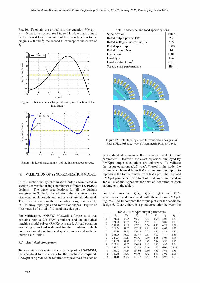
Fig. 10. To obtain the critical slip the equation Ti(s,δ′s−π) = 0 has to be solved, see Figure 11. Note that scr mustbe the closest local maximum of the s− δ function to theorigin s = 0 and δ′s the second x-intercept of the curve ofTi.

0.0 0.5 1.0 1.5 2.0 2.5 3.0

δ (rad.)

20

15

10

5

0

5

10

15

20

25

Inst

anta

nous

Torq

ue

δs δ ′s

Ti(0 , δ)

Figure 10: Instantaneous Torque at s = 0, as a function of theload angle.

0.0 0.2 0.4 0.6 0.8 1.0

slip

25

20

15

10

5

0

5

10

15

20

Inst

anta

nous

Torq

ue Scr

Ti (s , δ ,s−π)

Figure 11: Local maximum scr, of the instantaneous torque.

3. VALIDATION OF SYNCHRONIZATION MODEL

In this section the synchronization criteria formulated insection 2 is verified using a number of different LS-PMSMdesigns. The basic specifications for all the designsare given in Table 1. In addition, the machines’ rotordiameter, stack length and stator slot are all identical.The differences among these candidate designs are mainlyin PM array topologies and rotor slot shapes. Figure 12illustrates 4 of a total of 13 candidate designs.

For verification, ANSYS’ Maxwell software suite thatcontains both a 2D FEM simulator and an analyticalmachine model solver (RMXprt) is used. A load equationemulating a fan load is defined for the simulation, whichprovides a rated load torque at synchronous speed with theinertia as in Table 1.

3.1 Analytical comparison

To accurately calculate the critical slip of a LS-PMSM,the analytical torque curves for the machine is required.RMXprt can produce the required torque curves for each of

Table 1: Machine and load specificationsSpecification ValueRated output power, kW 2.2Rated voltage (line-to-line), V 525Rated speed, rpm 1500Rated torque, Nm 14Frame size 100LLoad type FanLoad inertia, kg.m2 0.15Steady state performance IE4

Figure 12: Rotor topology used for verification designs: a)Radial Flux, b)Spoke-type, c)Asymmetric Flux, d) V-type

the candidate designs as well as the key equivalent circuitparameters. However, the exact equations employed byRMXprt torque calculations are unknown. To validatethe torque equations (A.7) to (A.9) used in the study, theparameters obtained from RMXprt are used as inputs toreproduce the torque curves from RMXprt. The requiredRMXprt parameters for a total of 13 designs are listed inTable 2 (See the Appendix for detailed definition of eachparameter in the table).

For each machine Tc(s), Tb(s), Ta(s) and Ts(δ)were created and compared with those from RMXprt.Figures 13 to 16 compare the torque plots for the candidatedesign 6. Clearly there is a good correlation between the

Table 2: RMXprt output parametersE0 Xd Xq R1 R′2 X1 X2

1 171.20 33.25 99.53 6.63 3.99 3.07 1.802 171.20 33.25 99.53 6.63 2.1 3.07 1.803 232.40 50.08 107.21 6.64 4.11 4.29 1.524 218.36 51.03 107.55 9.91 4.11 4.63 1.525 247.86 51.53 159.32 9.92 2.35 4.22 1.456 241.26 55.22 153.49 7.61 3.22 4.19 2.437 224.94 37.11 99.72 3.69 2.45 3.06 1.988 189.60 37.70 101.37 8.42 2.74 3.96 1.859 227.41 39.07 106.88 8.42 2.85 3.95 2.64

10 233.03 35.99 172.59 9.66 1.97 6.06 0.83211 166.92 37.14 164.94 9.30 3.35 5.61 1.5612 187.65 33.63 99.75 8.42 2.89 3.92 2.0613 181.16 28.32 101.37 8.43 2.47 3.92 1.63

24th Southern African Universities Power Engineering Conference, 26 - 28 January 2016, Vereeniging, South Africa.

7B-1

0.0 0.2 0.4 0.6 0.8 1.0

slip

10

0

10

20

30

40

50

60

Cage T

orq

ue (

N)

Tc: RMXprt

Tc: Analytical

Figure 13: Torque curve comparison of Tc

0.0 0.2 0.4 0.6 0.8 1.0

slip

12

10

8

6

4

2

0

Bra

king T

orq

ue (

N)

Tb: RMXprt

Tb: Analytical

Figure 14: Torque curve comparison of Tb

results from equations (A.7) to (A.9) and RMXprt. Thesame was found to be true for the remaining 12 candidatedesigns, which means that these torque equations ofLS-PMSMs can be used to solve eqn. (2b).

3.2 Synchronization comparison

In this section the synchronization capabilities of all 13candidate designs are inspected with the proposed fan load.The analytical synchronization criteria model is applied toeach candidate design and the results are verified by usingANSYS’ Maxwell 2D transient FEM solver.

In 2D FEM, a load equation can be include in the transienttime-step simulation set-up. This was done by defining the

0.0 0.2 0.4 0.6 0.8 1.0

slip

20

10

0

10

20

30

40

50

Avera

ge T

orq

ue (

N)

Ta: RMXprt

Ta: Analytical

Figure 15: Torque curve comparison of Ta

0.5 0.0 0.5 1.0 1.5 2.0 2.5 3.0 3.5

δ (rad)

15

10

5

0

5

10

15

20

25

30

Synch

ronous

Torq

ue (

N)

Ts: RMXprt

Ts: Analitical

Figure 16: Torque curve comparison of Ts

0.0 0.5 1.0 1.5 2.0 2.5

time (s)

500

0

500

1000

1500

2000

Speed (

rd/s

)

Synch: 2D-FEM

Not synch: 2D-FEM

Figure 17: Synchronized vs non-synchronized FEM simulationrepresentations, where design 1 in blue, design 2 in yellow.

load equation as Tl = 14(1− (157.08−ωr)/157.08)2 withωr referring to the rotors angular velocity in rad/s. Thesystem inertia (Jl) was set at 0.15 kg.m2 and a time-step of1 ms was used in the analyses. Using the results from thesimulations both speed vs. time and instantaneous torquevs. speed graphs are compiled for each candidate design.Figure 17 represents two cases (designs 1 and 2) obtainedfrom the simulation results. The simulation results areinterpreted as follows:

• A machine is seen as synchronized once the rotationalspeed settles at 1500 rpm (yellow line);

• A machine is seen as not synchronized when therotational speed oscillates at a point below 1500 rpm(blue line).

Figures 18 and 19 are the instantaneous torque vs. speedplots for the two cases. It can be seen that it closelyresembles that of Figures 6 and 7 in Section 2 that wasobtained using the proposed analytical approach.

The comparison for all the candidate designs is presentedin Table 3. The synchronization state of a design isindicated under the method used. The first coulomb fromthe right states if the result of the proposed method matchesthat of ANSYS Maxwell 2D FEM. From the table it is clearthat a 100% match was achieved.

24th Southern African Universities Power Engineering Conference, 26 - 28 January 2016, Vereeniging, South Africa.

7B-1

500 0 500 1000 1500 2000

mechanical speed

100

50

0

50

100

150

Inst

anta

neous

Torq

ue (

N)

Ti: 2D-FEM

Figure 18: Torque vs speed characteristics obtained from FEM(design 2).

200 0 200 400 600 800 1000 1200 1400

mechanical speed

100

50

0

50

100

150

Inst

anta

neous

Torq

ue (

N)

Ti: 2D-FEM

Figure 19: Torque vs speed characteristics obtained from FEM(design 1).

4. CONCLUSION

This paper revisits the energy based synchronizationcriteria as presented in past literature. An improved andmore consistent approach for the study of synchronizationby using an energy based synchronization criteria modelhas been presented. Using an implicit non-linear solver,we have shown how to determine the s − δ planefunction, which can then be used to evaluate the state ofsynchronization. Despite the simplicity of the algorithmit provides highly accurate result with a large order ofconvergence. Indeed even the most popular numericalsolvers such as the finite element method rarely canprovide a second order of convergence, whereas thealgorithm used in our case has five order of convergence.

The new approach was verified by means of comparisonagainst 2D FEM transient time-step simulation andan alternative analytical LS-PMSM machine simulationtool. Results proved to compare well and as a resultthe proposed method can be deemed valid for theuse of synchronization estimation during the design ofLS-PMSMs. It does however still require experimentalvalidation. This can be done by implementing theproposed method during the design of LS-PMSM in futurework and as a result also limit the use of time-stepsimulations and decreasing design optimization time.

Table 3: Verification resultsID Synchronize? 2D FEM Analytical Match1 Synchronize? no no X2 Synchronize? yes yes X3 Synchronize? yes yes X4 Synchronize? no no X5 Synchronize? no no X6 Synchronize? yes yes X7 Synchronize? yes yes X8 Synchronize? yes yes X9 Synchronize? no no X10 Synchronize? no no X11 Synchronize? no no X12 Synchronize? no no X13 Synchronize? no no X

REFERENCES

[1] Honsinger, V.B., ”Permanent magnet machines:asynchronous operation,” IEEE Trans on PowerApparatus and Systems, PAS-99(4): 1503-1509, July1980.

[2] Miller, T.J.E., ”Synchronization of line-start perma-nent magnet AC motors,” IEEE Trans on PowerApparatus and Systems, PAS-103(7): 1822-1828,July 1984.

[3] Rahman, M.A., Osheiba, A.M., Radwan, T.S.,”Synchronization process of line-start permanentmagnet synchronous motors”, Electric Machines andPower Systems, 24(6):77-592, 1997.

[4] Isfahani, A.H., Vaez-Zadeh, S., Rahman, M.A.,”Evaluation of synchronization capability in line startpermanent magnet synchronous motors,” IEEE Inter-national Electric Machines and Drives Conference(IEMDC), pp.1346-1350, 15-18 May 2011.

[5] Rabbi, S.F., Rahman, M.A., ”Critical criteria forsuccessful synchronization of line-start IPM motors”, IEEE Journal of Emerging and Selected Topics inPower Electronics , 2(2):348-358, June 2014.

[6] Soulard, J., Nee, H.P., ”Study of the synchronizationof line-start permanent magnet synchronous motors,”Conference Record of the 2000 IEEE IndustryApplications Conference, 1:424-431, 2000.

[7] Tang, R.Y. Modern Permanent Magnet Machines:Theory and Design, China Machine Press, Beijing,December 1997.

24th Southern African Universities Power Engineering Conference, 26 - 28 January 2016, Vereeniging, South Africa.

7B-1

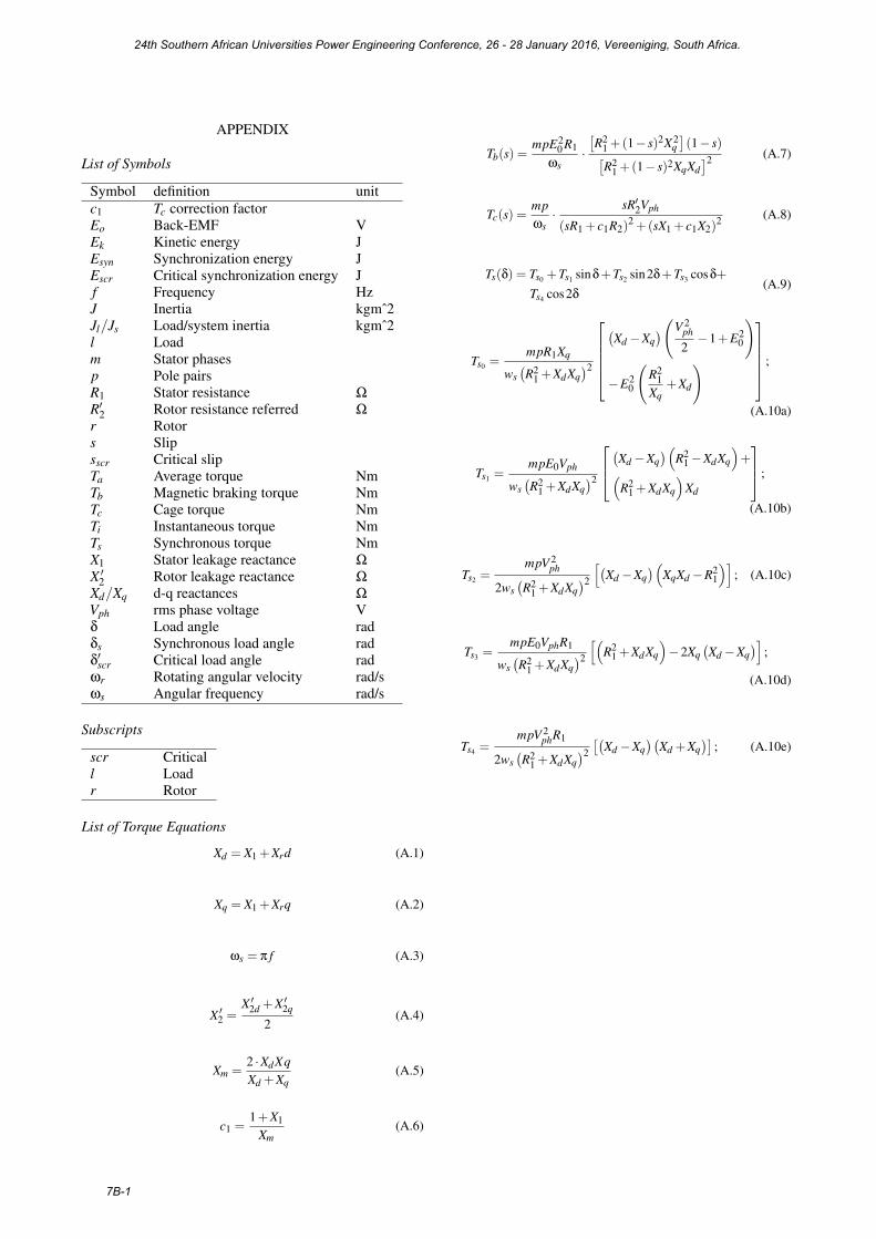
APPENDIX

List of Symbols

Symbol definition unitc1 Tc correction factorEo Back-EMF VEk Kinetic energy JEsyn Synchronization energy JEscr Critical synchronization energy Jf Frequency HzJ Inertia kgmˆ2Jl/Js Load/system inertia kgmˆ2l Loadm Stator phasesp Pole pairsR1 Stator resistance Ω

R′2 Rotor resistance referred Ω

r Rotors Slipsscr Critical slipTa Average torque NmTb Magnetic braking torque NmTc Cage torque NmTi Instantaneous torque NmTs Synchronous torque NmX1 Stator leakage reactance Ω

X ′2 Rotor leakage reactance Ω

Xd/Xq d-q reactances Ω

Vph rms phase voltage Vδ Load angle radδs Synchronous load angle radδ′scr Critical load angle radωr Rotating angular velocity rad/sωs Angular frequency rad/s

Subscripts

scr Criticall Loadr Rotor

List of Torque Equations

Xd = X1 +Xrd (A.1)

Xq = X1 +Xrq (A.2)

ωs = π f (A.3)

X ′2 =X ′2d +X ′2q

2(A.4)

Xm =2 ·XdXqXd +Xq

(A.5)

c1 =1+X1

Xm(A.6)

Tb(s) =mpE2

0 R1

ωs·[R2

1 +(1− s)2X2q](1− s)[

R21 +(1− s)2XqXd

]2 (A.7)

Tc(s) =mpωs· sR′2Vph

(sR1 + c1R2)2 +(sX1 + c1X2)

2 (A.8)

Ts(δ) = Ts0 +Ts1 sinδ+Ts2 sin2δ+Ts3 cosδ+

Ts4 cos2δ(A.9)

Ts0 =mpR1Xq

ws(R2

1 +XdXq)2

(Xd −Xq

)(V 2ph

2−1+E2

0

)

−E20

(R2

1Xq

+Xd

) ;

(A.10a)

Ts1 =mpE0Vph

ws(R2

1 +XdXq)2

(Xd −Xq

)(R2

1−XdXq

)+(

R21 +XdXq

)Xd

;

(A.10b)

Ts2 =mpV 2

ph

2ws(R2

1 +XdXq)2

[(Xd −Xq

)(XqXd −R2

1

)]; (A.10c)

Ts3 =mpE0VphR1

ws(R2

1 +XdXq)2

[(R2

1 +XdXq

)−2Xq

(Xd −Xq

)];

(A.10d)

Ts4 =mpV 2

phR1

2ws(R2

1 +XdXq)2

[(Xd −Xq

)(Xd +Xq

)]; (A.10e)

24th Southern African Universities Power Engineering Conference, 26 - 28 January 2016, Vereeniging, South Africa.

7B-1