Challenges of Turbocharging a Two-Cylinder Engine A...

Challenges of Turbocharging a Two-Cylinder Engine – A Computational Analysis of a Turbocharger Turbine by Transient CFD Methods

Valerius Boxberger1*, Roland Baar1, Maike Gern1, Rainer Zimmermann1

ISROMAC 2016

International

Symposium on

Transport

Phenomena and

Dynamics of

Rotating Machinery

Hawaii, Honolulu

April 10-15, 2016

Abstract

Drive train development is facing demands for reduced emissions and growing expectations for driving

dynamics coupled with declining fuel consumption. Downsizing in combination with turbocharging is a key

technology to ensure increased power density and efficiency, at reduced emission levels. Up to now, quasi-

steady behavior of the turbocharger has been assumed in the turbocharger design. However, the inflow

conditions for radial turbines are actually quite different for real pulsating engine operations, compared to

steady and quasi-steady conditions [1]. The aim of reducing the fuel consumption with fewer cylinders leads

to a further change in the boundary conditions for the turbocharger [7]. As a result, the quasi-steady

behavior, especially in two cylinder engines, does not seem to be valid and this has to be taken into account

during the design process [2], [3].

This paper presents a numerical investigation of a pulse charged turbocharger turbine to gain an

understanding of the aerodynamics at different pulse frequencies. A validated CFD-model is used to

compute two and four-cylinder pulses. The time dependent boundary conditions for pressure and

temperature are generated via 1D simulation. To make both pulse frequencies comparable, the turbine

simulations were run with the same specific exhaust cycle enthalpy.

The analyses of the results shows a significant deterioration of the turbine operating behavior at low

end torque due to the pulsating inflow of a two cylinder pulse compared to a four cylinder pulse. Higher

engine speeds reduce the disadvantages. Furthermore it can be shown that the storage effect of the

volute and the phase shift in temperature and pressure influences the throughput behavior of the

turbine. For that the specific pulsating flow conditions must be considered for an optimization of the

turbocharger of a two-cylinder engine.

Keywords

Turbocharging — Pulsating inflow — CFD

1 Department of Internal Combustion Engines, Technical University Berlin, Berlin, Germany

*Corresponding author: [email protected]

INTRODUCTION

More stringent emissions standards and a reduction in fuel consumption represent the major challenges for automotive industry. Displacement reduction is considered to be a suitable way to achieve the legal requirements. Schernus et. al [9] shows that the lowest CO2 emissions for vehicles with an inertia class less than 1130 kg occur at a displacement of 0.8 liter. Two-cylinder engines are at advantage because of their better single-cylinder volume and due to this light consumption benefits compared to three-cylinder engines.

The radial turbines operate under strongly non-steady exhaust pulses. The boundary conditions of a turbocharger turbine therefore changes depending on the engine firing frequency [4].

Furthermore, it has been found that test bench measurements do not match the pulsed conditions. Deviations of cycle averaged turbine performance; the efficiency and the mass flow rate differ from stationary measured turbochargers [2]. This makes an accurate the turbocharger modeling in the 1D simulation very complex. For two-cylinder engines, the pulsating exhaust gas flow has a particularly higher priority, since the bigger fluctuations in

the pressure of the exhaust gas, the mass flow and the temperature have a far greater impact on the turbocharger behavior than for engines with more than two cylinders. Real engine conditions are difficult to realize on turbocharger test benches. The experimental measurement of high-frequency temperatures and mass flows is still a major problem [1]. This can be attributed to the thermal inertia during temperature measurements. A reliable measurement of the data can still not be carried out satisfactorily. Changes in the flow direction of the fluid further complicate the measurements.

A detailed numerical analysis of the inlet conditions on a radial turbocharger turbine is performed. First a steady state validation with experimental test bench data is done. Furthermore transient real engine boundary conditions are generated for a two-cylinder engine in three different operating points via 1D simulation. Additionally, three artificial four-cylinder engine boundary conditions are generated which allow the usage as a reference to quantify the transient two-cylinder pulse turbine performance.

1 EXPERIMENT

Numerical methods such as 1D and 3D simulations require a

mailto:[email protected]

Challenges of Turbocharging a Two-Cylinder Engine – A Computational Analysis of a Turbocharger Turbine by Transient CFD

Methods — 2

preliminary validation of the models. In this context, both the engine and the turbocharger used were stationary measured on test benches (engine and turbocharger).

1.1 Test engine A 0.8 liter two-cylinder diesel engine with a performance

power of 35 kW was used for the validation of the 1D

simulation model. During the test bench measurements, the

speed of the turbocharger, the stationary pressure and

temperature were measured before and after the turbine for

different engine operating points. The pressure signal was

measured with high temporal resolution using pressure

quartz at the same place as the steady-state values. The

measurement result has been used for the validation of 1D

simulation engine model. Figure 1 shows the pressure

gradient over the crank angle in addition, the valve lift is

shown. More engine details can be found in [10].

1.2 Test turbocharger The turbocharger used is currently the smallest available

turbocharger on the market for diesel engines (type

designation: GT0632SZ, manufactured by the company

Honeywell Turbo Technologies). It is controlled via a waste

gate. The diameter of the turbine impeller is 30 mm, the

diameter of the compressor wheel is 32 mm. For the present

study, a standard map on the hot-gas test bench for

turbochargers was measured at the Department of Internal

Combustion Engines at the TU Berlin with a turbine inlet

temperature of Tturbine inlet = 600°C. Furthermore a second

adiabatic map was measured for the validation of the CFD

model.

Figure 1: Pressure indication before and after turbine

Finally a sensitivity analysis of the pulse was carried out. In

this, an artificial pressure pulse was generated by a cylinder

head which was fed with compressed air. Different pulses

frequencies could be modeled by changing the speed of the

camshaft. The sensitivity analysis was used to examine the

influence of the pulse frequency on the turbocharger speed. 2 NUMERICS METHODS AND VALIDATION

The detection of high-frequency flow phenomenon can currently be detected only on the numerical path. For this

reason, a stationary model is presented here. This corresponds geometrically exact to the turbocharger test bench. Additionally a second transient model is presented. This uses the same mesh for the impeller and the housing, only the inlet and the outlet have been changed to save simulation time. The transient simulations run with 1D simulation generated boundary conditions and for this does not require the test bead measuring tubes (inlet and outlet). 2.1 Numerical model The flow calculations of the turbocharger are based on a finite volume approach for solving steady and unsteady RANS/ URANS equations (Reynolds-Averaged-Navier-Stokes/ Unsteady-Reynolds-Averaged-Navier-Stokes).

The simulations were carried out with the commercial code ANSYS CFX, version 15.0.7. The tool uses an implicit discrete approach. The simulations were run with the setting high resolution which uses the second order backward Euler scheme when it is required to maintain a bounded solution it switch to the first order backward Euler.

The SST-turbulence model (SST = shear stress transport) was used in combination with the wall function. The transfer of information between the rotating and stationary domains was carried out by the frozen-rotor approach, which has been proven by [1] and [6] for steady and transient simulation. The walls were modelled as adiabatic and ideally smooth and the turbulence intensity was set to 5%. The break up criterion for the simulations has been set to the maximum residuals

(Rmax = 1.0 ∙ 10−3). During the simulation the mass flow, pressure ratio and the temperatures at the inlet and outlet was monitored. Table 1 shows the mesh types which were used for the discretization. Stationary CFD model: The test bench structure is modelled as shown in Figure 2 (left). The time step is calculated as follows:

time step =1

ωTC

(1)

ωTC describes the turbochargers angular velocity. Measuring tubes and the manifold was integrated into the model to consider the right pressure loss in the system. In addition a mesh independence study was carried out.

Table 1: Mesh overview

stat. model trans. model

inlet (hexa)

manifold (tetra)

volute (tetra)

impeller (hexa)

body (tetra)

outlet (hexa)

volute (tetra)

impeller (hexa)

body (tetra)

outlet (hexa)

The operating points were set by specifying a constant total

temperature, total pressure at the inlet and a static pressure at

the outlet. The data for the boundary conditions was imported

from the adiabatic turbocharger test bench measurements.

Finally the turbocharger speed and the material values for

exhaust gas were set.

Transient CFD model: The boundary conditions for the

transient simulation were derived from 1D simulation (crank

angle resolved). They are modelled as a time dependent

function. The temporally varying total pressure and the

Cyl. 1Cyl. 2

Cyl. 1Cyl. 2

Cyl. 1Cyl. 2

OP:1

OP:2

OP:3

CA [°]

-360 -300 -240 -180 -120 -60 0 60 120 180 240 300 360

Valv

e L

ift

[%]

0

20

40

60

80

100

120

Valv

e L

ift

[%]

0

40

80

120

Valv

e L

ift

[%]

0

40

80

120

Pre

ssure

[bar]

1.0

2.0

3.0

4.0

pbefor Turbine pafter Turbine OV fix OV var. IV fix

Pre

ssure

[bar]

1.0

2.0

3.0

4.0

Pre

ssure

[bar]

1.0

2.0

3.0

4.0


Methods — 3

temporally varying total temperature were set at the volute

inlet, see Figure 3.

Figure 2: 2.3 million model (left), 1.0 million model (right)

At the outlet, a constant steady pressure was defined. The

prior evaluation of the engine tests showed that the rotational

speed of the turbocharger during the 2C engine operation

varies by less than 1%, see Figure 4. The variation during

the 4C operating is estimated to be even lower. For that, the

turbocharger speed was set as constant.

Figure 3: Boundary conditions transient simulation

The time steps were adjusted to the operating point. Since

the simulation was run with the frozen rotor approach only

the pulse frequency had to be resolved which led to a bigger

time step. For the different operating points the time step has

been set as follows: ΔtOP1=8.0 ∙ 10−5𝑠, ΔtOP2=6.85 ∙ 10−5𝑠,

and ΔtOP3=5.33 ∙ 10−5𝑠. The transient simulations were

calculated with the 1.0 million mesh model. It has been used

in order to decrease simulation time. Figure 2 (right) shows

it. The initial conditions for the transient simulated were

taken from a previous calculated steady state simulation.

2.2 Validation High temperatures on the turbine side affect the oil in the bearing housing and also the compressed fresh air on the compressor side during the experimental measurement. It thus acts directly on the experimental determined efficiency.

Figure 4: TC speed reduction

Since an accurate numerical simulation of heat transfer in the

turbocharger is hard to achieve (detailed solid temperature,

solid materials and y+=1-2 required) commonly adiabatic

validation are carried out. In this case adiabatic conditions

could be reached by aligning the temperature of fluid in the

compressor, the turbine and the oil temperature to reduce

heat flux (TT,inlet = TOil = T𝐶,𝑜𝑢𝑡𝑙𝑒𝑡). In this way, nearly

adiabatic conditions are achieved for the turbocharger test

bench measurements.

Figure 5: Validation of the mass flow

To ensure a sufficient mesh density a grid independence

study was carried out. Every domain of the turbocharger

model was refined separately. The density was increased until

the changes in the monitored values were negligible. The

employed RANS code uses a wall-function for the boundary

layer resolution. To ensure an optimum functionality of it, at

least 10 nodes were places in the boundary layer. A preferably

small model was needed for keeping the transient simulation

feasible in a reasonable time.

The validation shows the qualification of the 2.3-million nodes

mesh for further investigations. To quantify the error of the

2.3-million-model a second model with a doubled mesh

number has been generated. The two models were compared

to each other. Only small deviations could be observed

between the integral values (reduced mass flow rate and a

deviation in the turbine efficiency of less than 2%, see Figure

5. The detailed analysis of the internal velocity distribution

OP:3

OP:1

OP:2

OP:1

OP:3

OP:2

OP:1

OP:3

OP:1

OP:3

2 Cylinder

4 CylinderCA [°]

-180 -120 -60 0 60 120 180

CA [°]

-180 -120 -60 0 60 120 180

p3t [b

ar]

1.0

1.5

2.0

2.5

3.0

3.5

4.0

T3t [°

C]

400

600

800

1000

1200

OP:2

OP:2

CA [°]

-180 -120 -60 0 60 120 180

CA [°]

-180 -120 -60 0 60 120 180

p3t [b

ar]

1.0

1.5

2.0

2.5

3.0

3.5

4.0

T3t [°

C]

400

600

800

1000

1200

1%

nEngine [1/min]

400 600 800 1000 1200 1400 1600

rpm

variation [

%]

0

2

4

6

8

10

12

turbocharger test bench:nTC=150.000 1/min

nA

TL [

1/m

in]

150000

152000

154000

156000

158000

160000

°CA

-360 -240 -120 0 120 240 360

engine test bench:nEngine=1500 1/min

1%

PT(t-s)

1.4 1.6 1.8 2.0 2.2 2.4 2.6

MF

P

0.38

0.40

0.42

0.44

0.46

0.48

TC test bench (adiabatic) CFD 2.3 mil. nodes CFD 3.8 mil. nodes

hT=h

T.is*h

m

0.40

0.44

0.48

0.52

0.56

0.60

8800 min-1*K-0,5

nTC,red=7670 min-1*K-0,5

10000 min-1*K-0,5

10950 min-1*K-0,5


Methods — 4

shows minor deviations, Figure 6. These were accepted to

shorten the computation time.

Figure 6: Internal velocity distribution

3 TRANSIENT BOUNDARY CONDITIONS

To create a valuation basis for the operating behavior of the

turbine during a 2C pulse, an additional artificial 4C pulse

was modeled. A 4C pulse was selected as reference

because of its high acceptance in the European market. Due

to this a 4C pulse counts as the standard operating

conditions for turbochargers. Two exhaust characteristics

(2C and 4C) were calculated for three engine operating

points.

The investigation of the thermodynamic behavior of the gas

turbine requires highly resolved pressure and temperature

gradients of the exhaust gas over time. These are set as

boundary conditions for the numerical simulation. Because of

the problematic detection of the experimental data, a 1D

simulation model of the 2C engine was used. The model had

previously been validated with the engine test bench data.

Three different operating points of the 2C engine were

calculated.

Table 2. Investigated engine operating points

OP #.

rpmEngine

[1/min]

pme

[bar]

rpmTC

[1/min]

1

2

3

1500

1750

2250

12.6

6.85

18.6

155.000

125.000

255.000

The artificial 4C pulse could be created by firstly adjusting the ignition angle. A change was made from 360 °CA (2C) to 180° CA (4C). Eq. 2 shows the approach for determining the specific exhaust gas enthalpy, equal to [8].

hexhaust,tt = h tt,3−4

= ∫ cp,3 ∙ T3t(φ) [1 − (p4t(φ)

p3t(φ))

κ−1κ

]720°

0°

∙ dφ

(2)

In addition the total inlet pressure and the total inlet

temperature were integrated over a cycle and then scaled

down to the level of the 2C pulse, see Eq. 3-7. As a result a

4C pulse with specific cycle exhaust gas enthalpy of a 2C

engine was created.

p3t,2 Cyl = ∫ p3t(φ)720°

0°

∙ dφ (3)

T3t,2 Cyl = ∫ T3t(φ)720°

0°

∙ dφ (4)

For both engine pulses, an equal turbocharger speed was set

for equal operating points. The mass flow of the turbine

adjusts itself according to expansion ratio and the efficiency.

p3t,2 Cyl = p3t,4 Cyl (5)

T3t,2 Cyl = T3t,4 Cyl (6)

hexhaust,tt,2 Cyl = hexhaust,tt,4 Cyl (7)

Dispersed engine operating points were selected to represent

a wide operating range on the engine performance map. The

selected points can be seen in Table 2. The first operating

point (OP: 1) is a full load point at lower engine speed (1500

rpm), while OP: 2 is a partial load point (1750 rpm) and OP: 3

describes the point with the maximum torque (2250 rpm).

Figure 7: specific exhaust enthalpy

Figure 7 (left) shows the specific enthalpy gradients over the crank angle. The variations of enthalpy during a working cycle can be seen. The full load point shows the greatest variations. Figure 7 (right) shows the integrals of the specific exhaust gas enthalpy. The conformity of the integral values allows the use of these boundary conditions for further investigations.

4 RESULTS AND DISCUSSION

4.1 Aerodynamics Four-cylinder pulses show higher turbine mass flow rates; see

Figure 8. The through flow difference is most evident in OP: 1;

here the value is 28% higher compared to the 2C. The other

operating points differ in the order of 16%. Schernus et. al [7]

made comparable observations. They note that the turbine at

2C pulses seems to ‘’behave’’ smaller than at pulses with a

higher cylinder number. The reduced through flow can also be

seen in Figure 9. Here the reduced turbine mass flow rate is

plotted against the expansion ratio.

Heat transfer influences on the housing, speed variations and

temperature effects on the mass flow can be excluded

because of the adiabatic boundary conditions and the reduced

mass flow. Furthermore, the reduced turbine mass flow in all

operating points is shown. The red hysteresis loop represents

the system boundary in the sections 3-4 (complete stage) for

the 2C pulse. Additionally the black hysteresis loop represents

CA [°]

0 180 360 540 720

htt, 3-4

[kJ/k

g]

0

100

200

300

400

htt, 3-4

[kJ/k

g]

0

100

200

300

400

htt, 3-4

[kJ/k

g]

0

100

200

300

400

CA [°]

0 180 360 540 720

2 Cylinder, 4 Cylinder

OP:1

OP:2

OP:3

OP:1

OP:3

ò h

tt, 3-4

[kJ/k

g]

0

40000

80000

120000

160000

ò h

tt, 3-4

[kJ/k

g]

0

40000

80000

120000

160000

ò h

tt, 3-4

[kJ/k

g]

0

40000

80000

120000

160000

ò h

tt, 3-4

[kJ/k

g]

0

40000

80000

120000

160000

OP:2


Methods — 5

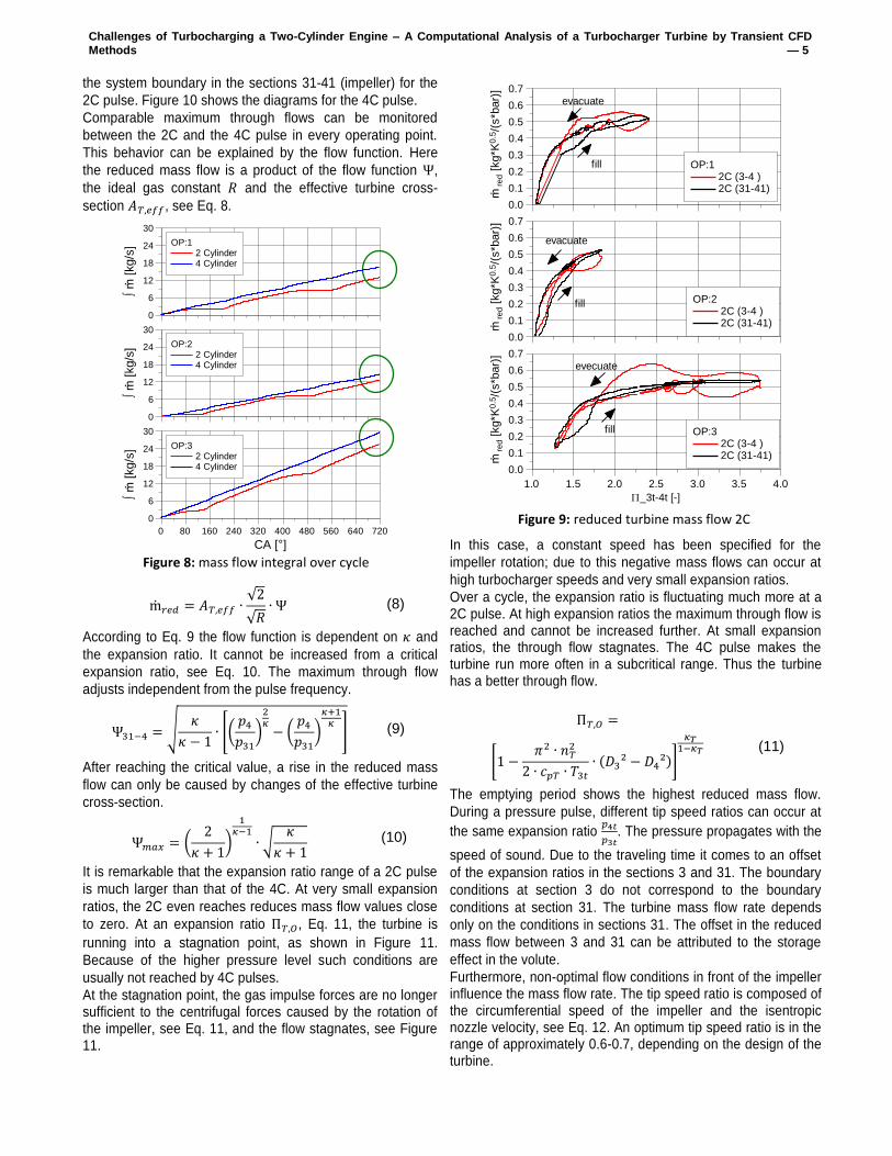
the system boundary in the sections 31-41 (impeller) for the

2C pulse. Figure 10 shows the diagrams for the 4C pulse.

Comparable maximum through flows can be monitored

between the 2C and the 4C pulse in every operating point.

This behavior can be explained by the flow function. Here

the reduced mass flow is a product of the flow function Ψ,

the ideal gas constant 𝑅 and the effective turbine cross-

section 𝐴𝑇,𝑒𝑓𝑓, see Eq. 8.

Figure 8: mass flow integral over cycle

m𝑟𝑒𝑑 = 𝐴𝑇,𝑒𝑓𝑓 ∙√2

√𝑅∙ Ψ (8)

According to Eq. 9 the flow function is dependent on 𝜅 and

the expansion ratio. It cannot be increased from a critical

expansion ratio, see Eq. 10. The maximum through flow

adjusts independent from the pulse frequency.

Ψ31−4 = √𝜅

𝜅 − 1∙ [(

𝑝4

𝑝31

)

2𝜅

− (𝑝4

𝑝31

)

𝜅+1𝜅

] (9)

After reaching the critical value, a rise in the reduced mass

flow can only be caused by changes of the effective turbine

cross-section.

Ψ𝑚𝑎𝑥 = (2

𝜅 + 1)

1𝜅−1

∙ √𝜅

𝜅 + 1 (10)

It is remarkable that the expansion ratio range of a 2C pulse

is much larger than that of the 4C. At very small expansion

ratios, the 2C even reaches reduces mass flow values close

to zero. At an expansion ratio Π𝑇,𝑂, Eq. 11, the turbine is

running into a stagnation point, as shown in Figure 11.

Because of the higher pressure level such conditions are

usually not reached by 4C pulses.

At the stagnation point, the gas impulse forces are no longer sufficient to the centrifugal forces caused by the rotation of the impeller, see Eq. 11, and the flow stagnates, see Figure 11.

Figure 9: reduced turbine mass flow 2C In this case, a constant speed has been specified for the

impeller rotation; due to this negative mass flows can occur at

high turbocharger speeds and very small expansion ratios.

Over a cycle, the expansion ratio is fluctuating much more at a 2C pulse. At high expansion ratios the maximum through flow is reached and cannot be increased further. At small expansion ratios, the through flow stagnates. The 4C pulse makes the turbine run more often in a subcritical range. Thus the turbine has a better through flow.

Π𝑇,𝑂 =

[1 −𝜋2 ∙ 𝑛𝑇

2

2 ∙ 𝑐𝑝𝑇 ∙ 𝑇3𝑡

∙ (𝐷3² − 𝐷4²)]

𝜅𝑇1−𝜅𝑇

(11)

The emptying period shows the highest reduced mass flow.

During a pressure pulse, different tip speed ratios can occur at

the same expansion ratio 𝑝4𝑡

𝑝3𝑡. The pressure propagates with the

speed of sound. Due to the traveling time it comes to an offset

of the expansion ratios in the sections 3 and 31. The boundary

conditions at section 3 do not correspond to the boundary

conditions at section 31. The turbine mass flow rate depends

only on the conditions in sections 31. The offset in the reduced

mass flow between 3 and 31 can be attributed to the storage

effect in the volute.

Furthermore, non-optimal flow conditions in front of the impeller influence the mass flow rate. The tip speed ratio is composed of the circumferential speed of the impeller and the isentropic nozzle velocity, see Eq. 12. An optimum tip speed ratio is in the range of approximately 0.6-0.7, depending on the design of the turbine.

ò ṁ

[kg/s

]

0

6

12

18

24

30

OP:1 2 Cylinder 4 Cylinder

ò ṁ

[kg/s

]

0

6

12

18

24

30


ò ṁ

[kg/s

]

0

6

12

18

24

30

CA [°]

0 80 160 240 320 400 480 560 640 720


ṁ r

ed [

kg*K

0.5

/(s*b

ar)

]

0.0

0.1

0.2

0.3

0.4

0.5

0.6

0.7

OP:1 2C (3-4 ) 2C (31-41)

evacuate

fill

ṁ r

ed [

kg*K

0.5

/(s*b

ar)

]

0.0

0.1

0.2

0.3

0.4

0.5

0.6

0.7

OP:2 2C (3-4 ) 2C (31-41)

evacuate

fill

evecuate

fill

ṁ r

ed [

kg*K

0.5

/(s*b

ar)

]

0.0

0.1

0.2

0.3

0.4

0.5

0.6

0.7

P_3t-4t [-]

1.0 1.5 2.0 2.5 3.0 3.5 4.0

OP:3 2C (3-4 ) 2C (31-41)


Methods — 6

Figure 10: reduced turbine mass flow 4C

Figure 11: stagnation point OP: 1

The tip speed ratio is an indicator for the optimum inflow angle. It affects both the turbine efficiency and the through flow performance.

𝑆31 =π ∙ D3 ∙ n𝑇

√2 ∙ cpT ∙ T31t ∙ [1 − (p41

p31t)

κ−1κ

]

(12)

Here the through flow is dependent on the effective turbine cross-section. The effective turbine cross-section can be determined as follows:

m𝑟𝑒𝑑,31 =m𝑇 ∙ √𝑇31𝑡

𝑝31𝑡

= 𝐴𝑇,𝑒𝑓𝑓 ∙√2

√𝑅

∙ Ψ (𝑝41

𝑝31𝑡

)

(13)

𝐴𝑇,𝑒𝑓𝑓 =m𝑟𝑒𝑑,31

√2

√𝑅∙ Ψ (

𝑝41

𝑝31𝑡)

(14)

According to [5] there is a relationship between the effective

turbine cross-section and the tip speed ratio. At constant expansion ratios, the effective turbine cross-section decreases with increasing speed ratio. Thus high tip speed ratios reduce the turbine through flow. The tip speed ratio depends on

cpT and κ and the total temperature. In accordance with the

numerical boundary conditions, cpT and κ can be considered

as constant. The temperature T31t and the expansion ratio p41

p31t change during a pressure pulse. The expansion ratio has

the greatest impact on the tip speed ratio.

Figure 12: Influence of the tip speed ratio (2C)

The comparison of the tip speed ratio in Figure 12 and Figure 13 show clearly the benefits of 4C pulse. The turbine is operating in a nearly constant tip speed ratio, close to the design point. Under 2C pulse the turbine is operating in poor regions, especially at low expansion ratios.

4.2 Specific power provision Due to the 1st main equation of turbocharging there is a equilibrium of power between turbine and compressor. Both are linked by a common shaft. In a steady state point the equilibrium determines the turbocharger speed. In a transient simulation a deviation of the compressor or turbine power leads to a change in turbocharger speed. Furthermore the equation for the equilibrium has to be expanded by the inertia power

which acts during acceleration or deceleration. The turbine power can be determined as follows:

PT = PC + PFr(+PIn) (15)

The power output of the turbine is in charge for the intake mass

flow, the specific heat capacities of the fluid and temperature. It

can be calculated as:

PT = ��𝑇 ∙ cp,exhaust ∙ (T3t − T4t) (16)

ṁre

d [

kg*K

0.5

/(s*b

ar)

]

0.0

0.1

0.2

0.3

0.4

0.5

0.6

0.7

OP:1 4C (3-4 ) 4C (31-41)

evacuate

fill

evacuate

fill

evacuate

fill

ṁre

d [

kg*K

0.5

/(s*b

ar)

]

0.0

0.1

0.2

0.3

0.4

0.5

0.6

0.7

OP:2 4C (3-4 ) 4C (31-41)

ṁre

d [

kg*K

0.5

/(s*b

ar)

]

0.0

0.1

0.2

0.3

0.4

0.5

0.6

0.7

P_3t-4t [-]

1.0 1.5 2.0 2.5 3.0 3.5 4.0

OP:3 4C (3-4 ) 4C (31-41)

ṁ3 [

kg/s

]

-0.01

0.00

0.01

0.02

0.03

0.04

0.05

0.06

0.07

CA [°]

0 60 120 180 240 300 360


ṁ3 [

kg/s

]

-0.01

0.00

0.01

0.02

0.03

0.04

0.05

0.06

0.07

CA [°]

0 60 120 180 240 300 360


P_31t-

41t

[-]

1.0

1.5

2.0

2.5

3.0

P_3t-4t [-]

1.0 1.5 2.0 2.5 3.0 3.5 4.0

ṁ r

ed [

kg*K

0.5

/(s*b

ar)

]

0.0

0.1

0.2

0.3

0.4

0.5

0.6

0.7

OP:3 2C (3-4 ) 2C (31-41)

storage effect

AT,eff

Sevacuate

Sfill

Pfill

Pevacuate

P=const P=const

S 3

1 [

-]

0.0

1.0

2.0

3.0

4.0

5.0

6.0

7.0


Methods — 7

Figure 13: Influence of the tip speed ratio (4C)

In the following the specific power output of the turbine will be

analyzed. To evaluate the specific power provision of the

radial turbine, the specific enthalpy over the entire turbine

stage was measured, see Figure 14.

The overall highest values for the turbine enthalpy can be

monitored at the 2C pulse. This is due to the partial higher

expansion ratio and temperature.

For both pulse frequencies very small or negative power

output could be determined. This can be traced back to small

expansion ratios and partly reversed flow for the 2C pulse.

The equation for the specific exhaust gas enthalpy is shown in

Eq. 17.

hT,is,tt = cp,exhaust ∙ (T3t − T4t) (17)

The consideration of enthalpy integral over the cycle shows

that the biggest advantages of the 4C pulse are at low speeds

and high loads. With increasing speed the specific enthalpy of

both pulses is equal.

The partially negative specific enthalpy of the 2C is

compensated to the higher speeds and higher inlet pressures

and temperatures.

4.3 Turbine efficiency

The determination of the isentropic efficiency under real

pulsating conditions represents a challenge and has been a

topic of research for many years; see [1], [2], [3], [4]. In this

chapter the problem of the determination of the temporal

resolved efficiency is demonstrated based on the operating

point BP: 3.

Turbine stage (section 4-3): The standard determination of

the pulsating efficiency leads to unphysical values as shown in

Figure 15.

Figure 14: Cycle integrated specific turbine power

Incorrect efficiency values are mainly due to storage effects.

These occur in the components of the turbine (e.g. volute

casing and turbine housing). Delayed gas exchange in the

volute affects the total temperature after the impeller; see

Figure 18 (top left).

ηT,is,tt =1 −

T4t

T3t

1 − (p4t

p3t)

κ−1κ

(18)

While the temperature 𝑇3𝑡 decreases in proportion to the

falling pressure (120 ° CA) the temperature 𝑇4𝑡 remains in this

area until 𝑇3𝑡 briefly falls below 𝑇4𝑡. The turbine housing is

filled with old hot exhaust gas at this point. When the

temperature of the gas is falling the mass flow is insufficient to

push out the old gas. The fresh cold gas mixes with the old

gas. A mixing temperature is measured at section 4, which

does not allow conclusions to be drawn about the turbine

efficiency.

Figure 15: Isentropical turbine efficiency section (3-4) (left),

section (31-41) (right)

P_31t-

41t

[-]

1.0

1.5

2.0

2.5

3.0

P_3t-4t [-]

1.0 1.5 2.0 2.5 3.0 3.5 4.0

ṁ r

ed [

kg*K

0.5

/(s*b

ar)

]

0.0

0.1

0.2

0.3

0.4

0.5

0.6

0.7

OP:3 4C (3-4 ) 4C (31-41)

storage effectS

31 [

-]

0.0

1.0

2.0

3.0

4.0

5.0

6.0

7.0

P=const

ò h

T, tt [

kJ/k

g]

-10000

0

10000

20000

30000

40000

50000

2 Cylinder, 4 Cylinder

OP:1

òhT

, tt [

kJ/k

g]

-10000

0

10000

20000

30000

40000

50000

OP:2

ò h

T, tt [

kJ/k

g]

-10000

0

10000

20000

30000

40000

50000

CA [°]

0 60 120 180 240 300 360

OP:3

hT.is>1

hT.is<0

hT

, tt [

J/k

g]

-50

50

150

250

350

450

550

exhaust (3-4) turbine (3-4)

hT

.is [

-]

-0.5

0.0

0.5

1.0

1.5

CA [°]

0 60 120 180 240 300 360

hT

, tt [

J/k

g]

-50

50

150

250

350

450

550

exhaust (31-41) turbine (31-41)

hT

.is [

-]

-0.5

0.0

0.5

1.0

1.5

CA [°]

0 60 120 180 240 300 360

hT.is>1


Methods — 8

Figure 16 shows the moment when the space behind the impeller is filled with warm gas and fresh cold gas is exiting the impeller. The efficiency becomes negative at this point.

Figure 16: Efficiency values eta<0 (cold filling)

Figure 17 shows the moment when the space behind the

impeller is filled with old cold gas and fresh warm gas is

entering the impeller. The old gas mixes with the fresh gas.

The resulting mixing temperature becomes lower than the

real turbine outlet temperature. The consequences are

isentropic efficiencies greater than one.

Figure 17: Efficiency values eta>1 (hot filling)

Turbine impeller (section 31-41): The influence of the

storage effects can be avoided by reducing the system

boundary to the sections 31-41. Figure 15 (right) and Figure

18 (right) show a corresponding attempt. The impeller can

be treated as quasi-stationary, [1], [2].

Figure 18: Temperature and mass flow behavior during a

pulse It shows no significant storage effects. The reduction of the

system boundary alone is not constructive. The pulsating

character of the exhaust gas flow causes another

phenomenon that distorts the efficiency consideration. The

turbine expansion ratio decrease until the stagnation point is

reached.

Figure 19: Temperature gradient at the stagnation point

The gas in front of the impeller starts recirculating and heats

up. 𝑇4𝑡,𝑖𝑠 increases in dependence to 𝑇3𝑡, and simultaneously

the pressure level decreases over the turbine. 𝑇31𝑡 remains

temporarily in the stagnation region at an elevated

temperature level, see Figure 19. This leads to isentropic

efficiencies greater than one.

5 CONCLUSION A numerical study of the turbine behavior of a turbocharger turbine at different engine pulse frequencies was carried out. The investigations were performed by transient 3D CFD simulations. A 2C engine pulse and a 4C pulse have been investigated. The artificial 4C pulse was created to give the analysis a quantitative reference.

2C engines have a doubled ignition angle compared to 4C engines. This results in a significantly increased time interval between the exhaust valve openings. The fluctuation of inlet pressure and temperature increases (more time for the impeller to reduce the pressure until the next valve opening). During this analysis the cycle averaged pressure and temperature and thus the specific exhaust enthalpy for both types of pulses were hold constant. As a result the pressure and temperature peaks were smaller at the 4C pulse (the pressure was spread over four instead of two cylinders.)

The analyses shows the biggest disadvantages of the 2C pulse in the area of low end torque. The variations in the expansion ratio are highest here. Small expansion ratios lead to stagnation or back flow, furthermore very high expansion ratios lead to choke. The influence on the cycle integrated reduced mass and specific power output is significant at high engine loads and small speeds. Operating points with higher engine speed reduce the 2C disadvantages.

The major finding in this paper is that the hysteresis loop is not only influenced by storage effects in the volute. Observing only the impeller in the system boundary does not make the hysteresis disappear. A second cause is the effect of phase shift in temperature and pressure in the volute. Upstream of the impeller the shift changes the blade speed ratio (high speed ratios lead to lower effective turbine cross-sections) and due to this reduces the swallowing capacity of the turbine.

The determination of the transient turbine efficiency is still a major problem. A reduced system boundary (only impeller)

T t [

K]

600

700

800

900

1000

1100

1200

T3 t

T4 t

T4 t, is

OP:3

ṁ [

kg/s

]

0.00

0.01

0.02

0.03

0.04

0.05

0.06

0.07

ṁ3

ṁ4

OP:3

P(t

-t) [-

]

1.0

1.5

2.0

2.5

3.0

3.5

4.0

CA [°]

0 60 120 180 240 300 360

OP:3

T t [

K]

600

700

800

900

1000

1100

1200

T31 t

T41 t

T41 t, is

OP:3

ṁ [

kg/s

]

0.00

0.01

0.02

0.03

0.04

0.05

0.06

0.07

ṁ31

ṁ41

OP:3

P(t

-t) [-

]

1.0

1.5

2.0

2.5

3.0

3.5

4.0

KW [°]

0 60 120 180 240 300 360

OP:3

CA [°]

0 60 120 180 240 300 360

T31 t [

K]

600

700

800

900

1000

1100

1200

OP:3

p31 t [

bar]

1.0

1.5

2.0

2.5

3.0

3.5

4.0


Methods — 9

eliminates the storage problem and is simply done by the CFD methods. During the investigations it is shown that this method is only valid for medium and high expansion ratios. The calculation of the transient efficiency close to the stagnation point is not possible. Due to reverse flow and friction caused heatup of the gas upstream the turbine impeller.

REFERENCES

[1] Aymanns, R. Scharf, J., Uhlmann, T., et al., A

Revision of Quasi Steady Modelling in the

Simulation of Pulse Charged Engines, 16.

Aufladetechnische Konferenz, September 2011

[2] Cao, T., Xu, L., Yang, M., et al., Radial Turbine

Rotor Response to Pulsating Inlet Flows, Journal of

Turbomachinery 2014, July 2014, Vol. 136/071003-1

[3] Lüddecke, B., Filsinger, D., Bargende, M., Engine

crank angle resolved turbocharger turbine

performance measurements by contactless shaft

torque detection, 11th International Conference on

Turbochargers and Turbocharging, May 2014

[4] Reuter, S., Koch, A., Erweiterung des

Turbinenkennfeldes durch ein innovatives

Messverfahren als Randbedingung für die

Ladungswechselsimulation, 15. Aufladetechnische

Konferenz, September 2010

[5] Pucher, P. Zinner K., Aufladung von

Verbrennungsmotoren, Springer Verlag, 4. Auflage,

February 2012

[6] Roclawski, H.; Gugau, M.; et al., Influence on

Degree of Reaction on Turbine Performance for

Pulsating Flow Conditions, ASME Turbo Expo, June

2014, GT2014-25829

[7] Schernus, C., Dietrich, C., Nebbia, C., et al.,

Turboaufladung für kleine Ottomotoren mit weniger

als vier Zylindern, Motorprozesssimulation und

Aufladung, III: Engine Process Simulation and Su-

percharging, May 2011

[8] Vogt, M., Aufladesysteme für Ottomotoren im

Vergleich, Dissertation, Fachgebiet

Verbrennungskraftmaschinen, Technische

Universität Berlin, December 2009

[9] Weinowski, R., Sehr, A., Wedowski, S., et al.,

Zukünftiges Downsizing bei Ottomotoren- Potentiale

und Grenzen von 2- und 3- Zylinder Konzepten, 30.

Internationales Wiener Motorsymposium, May 2009

[10] Zillmer, M., Hadler, J., Jelden, H., et al., The

Drivetrain for the New Volkswagen „1-Litre Car“,

20th Aachener Colloquium: Automobile and Engine

Technology 2011, October 2011

Challenges of Turbocharging a Two-Cylinder Engine A...

Documents

Transcript of Challenges of Turbocharging a Two-Cylinder Engine A...