Ch10 HMM Model 10.1 Discrete-Time Markov Process 10.2 Hidden Markov Models 10.3 The three Basic...

Ch10 HMM Model

• 10.1 Discrete-Time Markov Process

• 10.2 Hidden Markov Models

• 10.3 The three Basic Problems for HMMS and the solutions

• 10.4 Types of HMMS

• 10.5 Continuous observation Densities in HMMS

10.1 Discrete-Time Markov Process (1)

• A system at any time may be in one of a set of N distinct states indexed by {1,2,…,N}. The system undergoes a change of state (possibly back to the same state) according to a set of probability with the state.

• Time is represented by t=1,2,…, the state at t by qt.

Discrete-Time Markov Model (2)

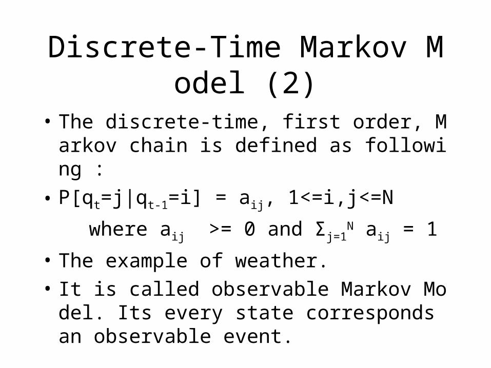
• The discrete-time, first order, Markov chain is defined as following :

• P[qt=j|qt-1=i] = aij, 1<=i,j<=N

where aij >= 0 and Σj=1N aij = 1

• The example of weather.

• It is called observable Markov Model. Its every state corresponds an observable event.


• By giving the state-transition matrix, it can answer a lot of questions.

• (1) What is the probability of a sequence of weather : Calculate P(O|Model) by

O = (sun,sun,sun,rain,rain,sun,cloudy,sun)

• (2) O = ( i, i, …i, j!=i )

1 2 d d+1


• What is the probability that the system is at state i for first d instances.

• pi(d)=(aii)d-1(1-aii)

• di = 1/(1-aii)

Hidden Markov Model (1)

• Extension : the observation is a probability function of the state.

• So there is a doubly embedded stochastic process : the underlying stochastic process is not directly observable(it is hidden), but can be observed only through another set of stochastic processes that produce the sequence of observations. The name comes.

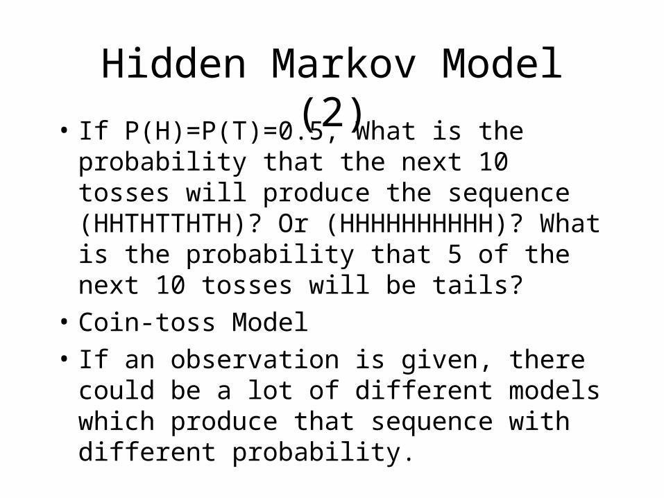
Hidden Markov Model (2)• If P(H)=P(T)=0.5, What is the probability

that the next 10 tosses will produce the sequence (HHTHTTHTH)? Or (HHHHHHHHHH)? What is the probability that 5 of the next 10 tosses will be tails?

• Coin-toss Model

• If an observation is given, there could be a lot of different models which produce that sequence with different probability.


• The Urn-and-Ball Model• There are a couple of urns in which there

are many balls with different colors.• If an observation sequence is given, there

are a lot of interpretation for it.• Here the urns are the states, the balls of

different color could be the observable events


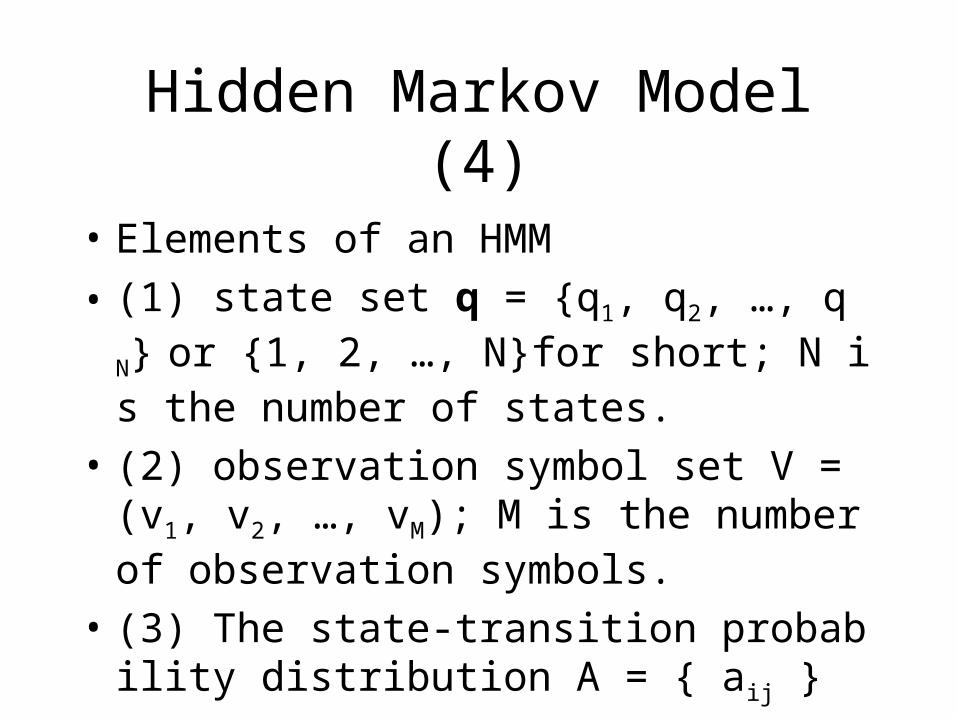
• Elements of an HMM

• (1) state set q = {q1, q2, …, qN} or {1, 2, …, N}for short; N is the number of states.

• (2) observation symbol set V = (v1, v2, …, v

M); M is the number of observation symbols.

• (3) The state-transition probability distribution A = { aij }


• aij = P[qt+1=j|qt=i] 1<=i,j<=N

• (4) The observation symbol distribution B={bj(k)} where bj(k) = P[ot=vk|qt=j] 1<=k<=M

• (5) The initial state distribution π={πi} where πi= P[q1=i] 1<=i<=N

• Sometime the model is presented by λ = ( A, B, π)


• If an HMM is given, it could be used as a generator to give an observation sequence O=(o1, o2, …, oT) where T is the number of observations, oi is one of the symbols from V (discrete case)

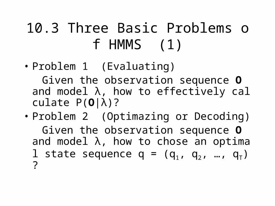
10.3 Three Basic Problems of HMMS (1)

• Problem 1 (Evaluating) Given the observation sequence O and mod

el λ, how to effectively calculate P(O|λ)? • Problem 2 (Optimazing or Decoding) Given the observation sequence O and mod

el λ, how to chose an optimal state sequence q = (q1, q2, …, qT) ?

Three Basic Problems of HMMS (2)

• Problem 3 (Training)

• How to adjust the model parameters • λ = ( A, B, π) to maximize P(O|λ)?

• The solution to problem 1• In fact, all possible state sequence will contr

ibute to P(O|λ). If a state sequence is :

• q = (q1, q2, …, qT)

Three Basic Problems of HMMS (4)• The Forward Procedure• Define αt(i) = P(o1, o2, …, ot, qt=i|λ) is the probabil

ity of the partial observation sequence, o1, o2, …, o

t, (until time t) and state i at time t, given the model λ.

• The Iterative procedure is as following :

(1) Initialization α1(i) = πibi(o1) 1<=i<=N

(2) Iteration αt+1(j) = [Σj=1Nαt(i)aij] bj(ot+1), t=1~T-1

(3) Termination P(O|λ) = Σi=1NαT(i)

• This procedure requires N2T calculations rather than 2TNT.

Three Basic Problems of HMMS (5)• The Backward Procedure

• Define βt(i) = P(ot+1, ot+2, …, oT| qt=i,λ) is the probability of the partial observation sequence from ot+1 to the end, given state i at time t and the model λ.

• The iterative procedure is as following :

(1) Initialization βT(i) = 1, 1<=i<=N

(2) Iteration βt(i) = Σj=1N aij bj(ot+1)βt+1(j), t=1~T-1

(3) Termination P(O|λ)= Σi=1N πiβ1(i)bi(o1)

• It also requires about N2T calculations.

Three Basic Problems of HMMS (6) • Solution to problem 2

• The first concept is how to define the ‘optimality’. The most widely used criterion is to find the single best state sequence ( path ) to maximize P(q|O,λ) which is equivalent to maximizing P(q,O|λ).

• The formal technique is based on dynamic programming methods and called Viterbi algorithm

• The Viterbi Algorithm

• Define δt(i) = max P(q1q2…qt-1, qt=i, o1 o2…ot|λ) for q1 q2…qt-1 is the best score along a path, at time t which accounts for the first t observations and ends in state i.


• δt+1(j) = max [δt(i)aij] bj(ot+1)

• The iterative procedure :

(1) Initialization δ1(i) = πibi(o1), ψ1(i)=0, i=1~N

(2) Iterationδt(j) = max [δt-1(i)aij] bj(ot) for i,j=1~N,t=2~T

ψt(j)= argmax [δt-1(i)aij], for i,j=1~N,t=2~N

• (3) Termination P* = maxi=1N [δT(i)]

ψT* = argmaxi=1

N [δT(i)]

• (4) Path backtracking qt* = ψt+1(qt+1

*) t=T-1~1

• An alterative Viterbi implementation uses logarithm to avoid underflow.


• Solution to Problem 3

• There is no analytic solution for that. Only iterative procedures are available, such as Baum-Welch method (or known as Expectation Maximization)

• Baum re-estimation procedure

• Define ξt(i,j) = P(qt=i, qt+1=j|O,λ)

• ξt(i,j) = P(qt=i, qt+1=j,O|λ)/P(O|λ)

=αt(i)aijbj(ot+1)βt+1(j)/ P(O|λ)

= αt(i)aijbj(ot+1)βt+1(j)/Σi=1NΣj=1

Nαt(i)aijbj(ot+1)βt+1(j)


• Define γt(i) = P(qt=i|O,λ) is the probability of being in state i at time t, given O and λ.

• γt(i) = P(qt=i,O|λ)/P(O|λ)

= P(qt=i,O|λ)/Σi=1N P(qt=i,O|λ)

= αt(i)βt(i)/ Σi=1Nαt(i)βt(i)

• So γt(i) = Σj=1Nξt(i,j)

• If we sum γt(i) over the time index t, we get the expected of times that state i is visited, or the expected number of transitions made from state i. The sum of ξt(i,j) over t is the expected number of transitions from i to j.


• So πj’ = γ1(j) , aij’ = Σt=1T-1ξt(i,j)/ Σt=1

T-1γt(i)

• bj’(k) = Σt=1Tγt’(j) / Σt=1

Tγt(j) t=1~T and the numerator only considers the cases that the observation ot is vk.

• These are the iterative formula for the model parameters.

• The initial parameters λ0 could be even distributions. Then

αt(i) and βt(i) (1<=i<=N, 1<=t<=T) could be calculated for

all samples, ξt(i,j) and γt(i) also could be calculated, so λgets updated as above.

10.4 Types of HMMS (1)

• Full connection A will be an n x n square matrix and all elements of A are not zero.

• But there are some different types. For example :

• The left-right HHM model. In this model the state index will be increased. For this model, aij = 0 for j<i and πi = 1 only for i=1, and aNN = 1, aNi = 0 for i<N.

• There could be some other types : more transfer with skip

10.5 Continuous Observation Densities in HMMS (1)

• In previous discussion we suppose the observation are discrete symbols. We must consider the continuous case.

• In this case, bj(k) will become probability density bj(o). The most general representation of the pdf is a finite mixture of the form

• bj(o) = Σk=1M cjkN(o, μjk,Ujk ) M is the number of d

istributions of the mixture, cjk > 0 and

Σk=1M cjk = 1, j=1~N

Continuous observation densities in HMMS (2)

• The re-estimation formulas are :

• cjk’ = Σt=1Tγt(j, k) / Σt=1

T Σk=1Mγt(j, k)

• μjk’ = Σt=1Tγt(j, k)*ot / Σt=1

T γt(j, k)

• Ujk’ = Σ t=1T γt(j, k)*(o-μjk) (o-μjk)’/ Σ t=1

T γt(j, k)

whereγt(j, k)=[αt(i)βt(i)/ Σi=1Nαt(i)βt(i)] *

[cjkN(o, μjk,Ujk )]/ Σk=1M cjkN(o, μjk,Ujk)]

Ch10 HMM Model 10.1 Discrete-Time Markov Process 10.2 Hidden Markov Models 10.3 The three Basic...

Documents

Transcript of Ch10 HMM Model 10.1 Discrete-Time Markov Process 10.2 Hidden Markov Models 10.3 The three Basic...