![Organizing [Compatibility Mode]](https://static.fdocuments.in/doc/165x107/553d1238550346e2498b4c66/organizing-compatibility-mode.jpg)
Ch01 Introduction Compatibility Mode
98
Introduction Introduction CHAPTER 1 1. .1 1 What is a signal? What is a signal? A signal is formally defined as a function of one or more variables that A signal is formally defined as a function of one or more variables that . . 1.2 What is a system? What is a system? A s stem i s f ormall defined as an enti t that mani ulates one or more A s stem i s f ormall defined as an enti t that mani ulates one or more signals to accomplish a function, thereby yielding new signals. signals to accomplish a function, thereby yielding new signals. Figure 1.1 (p. 2) oc agram representat on o a system. 1 1. .3 3 Overview of Specific Systems Overview of Specific Systems ★ .. 1 1. Analog communication system: modulator + channel + demodulator . Analog communication system: modulator + channel + demodulator Elements of a communication system Fig. Fig. 1 1. .2 2 Signals_and_Systems_Simon Haykin & Barry Van Veen 1
-
Upload
dechatorn-subcharoen -
Category
Documents
-
view
243 -
download
0
Transcript of Ch01 Introduction Compatibility Mode

8/13/2019 Ch01 Introduction Compatibility Mode
http://slidepdf.com/reader/full/ch01-introduction-compatibility-mode 1/98
IntroductionIntroductionCHAPTER
11..11 What is a signal?What is a signal?
A signal is formally defined as a function of one or more variables thatA signal is formally defined as a function of one or more variables that
. .
11..22 What is a system?What is a system?
A s stem is formall defined as an entit that mani ulates one or moreA s stem is formall defined as an entit that mani ulates one or more
signals to accomplish a function, thereby yielding new signals.signals to accomplish a function, thereby yielding new signals.
Figure 1.1 (p. 2)
oc agram representat on o a system.
11..33 Overview of Specific SystemsOverview of Specific Systems
★ .. ..
11. Analog communication system: modulator + channel + demodulator . Analog communication system: modulator + channel + demodulator
Elements of a communication system Fig.Fig. 11..22
Signals_and_Systems_Simon
Haykin & Barry Van Veen
1

8/13/2019 Ch01 Introduction Compatibility Mode
http://slidepdf.com/reader/full/ch01-introduction-compatibility-mode 2/98
IntroductionIntroductionCHAPTER
FigureFigure 11..22 (p.(p. 33))
Elements of a communication system. The transmitter changes the messageElements of a communication system. The transmitter changes the message
signal into a form suitable for transmission over the channel. The receiversignal into a form suitable for transmission over the channel. The receiver
processes the channel output (i.e., the received signal) to produce an estimateprocesses the channel output (i.e., the received signal) to produce an estimate
of the message signal.of the message signal.
Modulation:Modulation:
22. Di ital communication s stem:. Di ital communication s stem:
sampling + quantization + codingsampling + quantization + coding → transmitter transmitter → channelchannel → receiver receiver
Two basic modes of communication:Two basic modes of communication:
1.1. BroadcastingBroadcasting
2.2. PointPoint--toto--point communicationpoint communication
Radio, televisionRadio, television
Telephone, deep-space
Fig.Fig. 11..33
Signals_and_Systems_Simon
Haykin & Barry Van Veen
2
communication

8/13/2019 Ch01 Introduction Compatibility Mode
http://slidepdf.com/reader/full/ch01-introduction-compatibility-mode 3/98
IntroductionIntroductionCHAPTER
Figure 1.3 (p. 5)
(a) Snapshot of Pathfinder
ex lorin the surface of Mars.
(b) The 70-meter (230-foot)
diameter antenna located at
Canberra, Australia. The
surface of the 70-meter
reflector must remain accurate
within a fraction of the signal’s
wavelength. (Courtesy of JetPropulsion Laboratory.)
Signals_and_Systems_Simon
Haykin & Barry Van Veen
3
8/13/2019 Ch01 Introduction Compatibility Mode
http://slidepdf.com/reader/full/ch01-introduction-compatibility-mode 4/98
IntroductionIntroductionCHAPTER
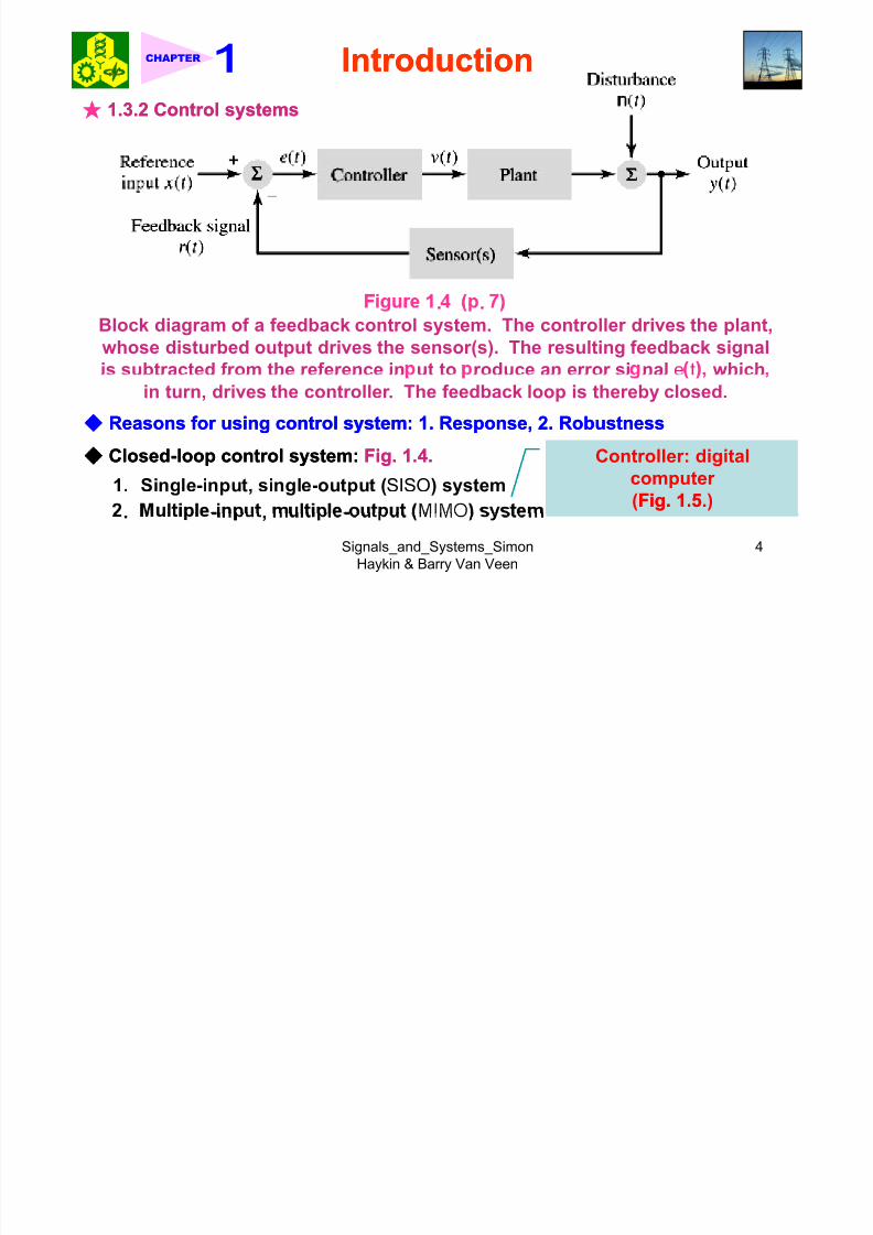
★ 11..33..22 Control systemsControl systems
. .
Block diagram of a feedback control system. The controller drives the plant,whose disturbed output drives the sensor(s). The resulting feedback signal
is subtracted from the reference in ut to roduce an error si nal e t which
in turn, drives the controller. The feedback loop is thereby closed.
Reasons for using control system:Reasons for using control system: 11. Response,. Response, 22. Robustness. Robustness ClosedClosed--loop control system:loop control system: Fig.Fig. 11..44..
1. Single-input, single-output (SISO) system
- -
Controller: digital
computer
(Fig.Fig. 11..55.)
Signals_and_Systems_Simon
Haykin & Barry Van Veen
4
. ,

8/13/2019 Ch01 Introduction Compatibility Mode
http://slidepdf.com/reader/full/ch01-introduction-compatibility-mode 5/98
IntroductionIntroductionCHAPTER
Figure 1.5 (p. 8)
NASA s ace shuttle launch.
(Courtesy of NASA.)
Signals_and_Systems_Simon
Haykin & Barry Van Veen
5

8/13/2019 Ch01 Introduction Compatibility Mode
http://slidepdf.com/reader/full/ch01-introduction-compatibility-mode 6/98
IntroductionIntroductionCHAPTER
★ 11..33..33MicroelectromechanicalMicroelectromechanical
Systems (Systems (MEMSMEMS))
Structure of lateral capacitiveStructure of lateral capacitive
accelerometers:accelerometers: Fig.Fig. 11--66 (a)(a)..
FigureFigure 11..66a (p.a (p. 88))
Structure of lateralStructure of lateralcapacitive accelerometers.capacitive accelerometers.
(Taken from Yazdi et al.,(Taken from Yazdi et al.,
Proc. IEEEProc. IEEE,, 19981998))
Signals_and_Systems_Simon
Haykin & Barry Van Veen
6

8/13/2019 Ch01 Introduction Compatibility Mode
http://slidepdf.com/reader/full/ch01-introduction-compatibility-mode 7/98
IntroductionIntroductionCHAPTER
SEM view ofSEM view of
Analog Device’sAnalog Device’s
--
micromachinedmicromachined
polysiliconpolysilicon
Fig.Fig. 11--66 (b).(b).
FigureFigure 11..66b (p.b (p. 99))SEM view of AnalogSEM view of Analog
Device’s ADXLODevice’s ADXLO55
surfacesurface--
micromachinedmicromachined
polysiliconpolysiliconaccelerometer.accelerometer.
(Taken from Yazdi et(Taken from Yazdi et
al.,al., Proc. IEEEProc. IEEE,, 19981998))
Signals_and_Systems_Simon
Haykin & Barry Van Veen
7

8/13/2019 Ch01 Introduction Compatibility Mode
http://slidepdf.com/reader/full/ch01-introduction-compatibility-mode 8/98
IntroductionIntroductionCHAPTER
★ 11..33..44 Remote SensingRemote SensingRemote sensing is defined as the process of acquiring information about an
object of interest without being in physical contact with it
1. Acquisition of information = detecting and measuring the changes that the
object imposes on the field surrounding it.. ypes o remo e sensor:. ypes o remo e sensor:
Radar sensor
Infrared sensor
Visible and near-infrared sensor X-ray sensor
SyntheticSynthetic--aperture radar (SAR)aperture radar (SAR)
Satisfactory operation See Fig.See Fig. 11..77
Ex. A stereo pair of SAR acquired from earth orbit with Shuttle Imaging Radar Ex. A stereo pair of SAR acquired from earth orbit with Shuttle Imaging Radar
SIRSIR--BB
Signals_and_Systems_Simon
Haykin & Barry Van Veen
8

8/13/2019 Ch01 Introduction Compatibility Mode
http://slidepdf.com/reader/full/ch01-introduction-compatibility-mode 9/98
IntroductionIntroductionCHAPTER
FigureFigure 11..77 (p.(p. 1111))
Perspectival view ofPerspectival view of
(California), derived(California), derived
from a pair of stereofrom a pair of stereo
from orbit with thefrom orbit with the
shuttle Imaging Radarshuttle Imaging Radar
SIRSIR--B . Courtes ofB . Courtes of
Jet PropulsionJet PropulsionLaboratory.)Laboratory.)
Signals_and_Systems_Simon
Haykin & Barry Van Veen
9

8/13/2019 Ch01 Introduction Compatibility Mode
http://slidepdf.com/reader/full/ch01-introduction-compatibility-mode 10/98
IntroductionIntroductionCHAPTER
★ 11..33..55 Biomedical Signal ProcessingBiomedical Signal ProcessingMorphological types of nerve cells:Morphological types of nerve cells: Fig.Fig. 11--88..
FigureFigure 11..88 (p.(p. 1212))
cortex, based on studies of primary somatic sensory and motor cortices.cortex, based on studies of primary somatic sensory and motor cortices.
(Reproduced from E. R. Kande, J. H. Schwartz, and T. M. Jessel,(Reproduced from E. R. Kande, J. H. Schwartz, and T. M. Jessel, Principles ofPrinciples of
Signals_and_Systems_Simon
Haykin & Barry Van Veen
10
,, .,., ..
8/13/2019 Ch01 Introduction Compatibility Mode
http://slidepdf.com/reader/full/ch01-introduction-compatibility-mode 11/98
IntroductionIntroductionCHAPTER
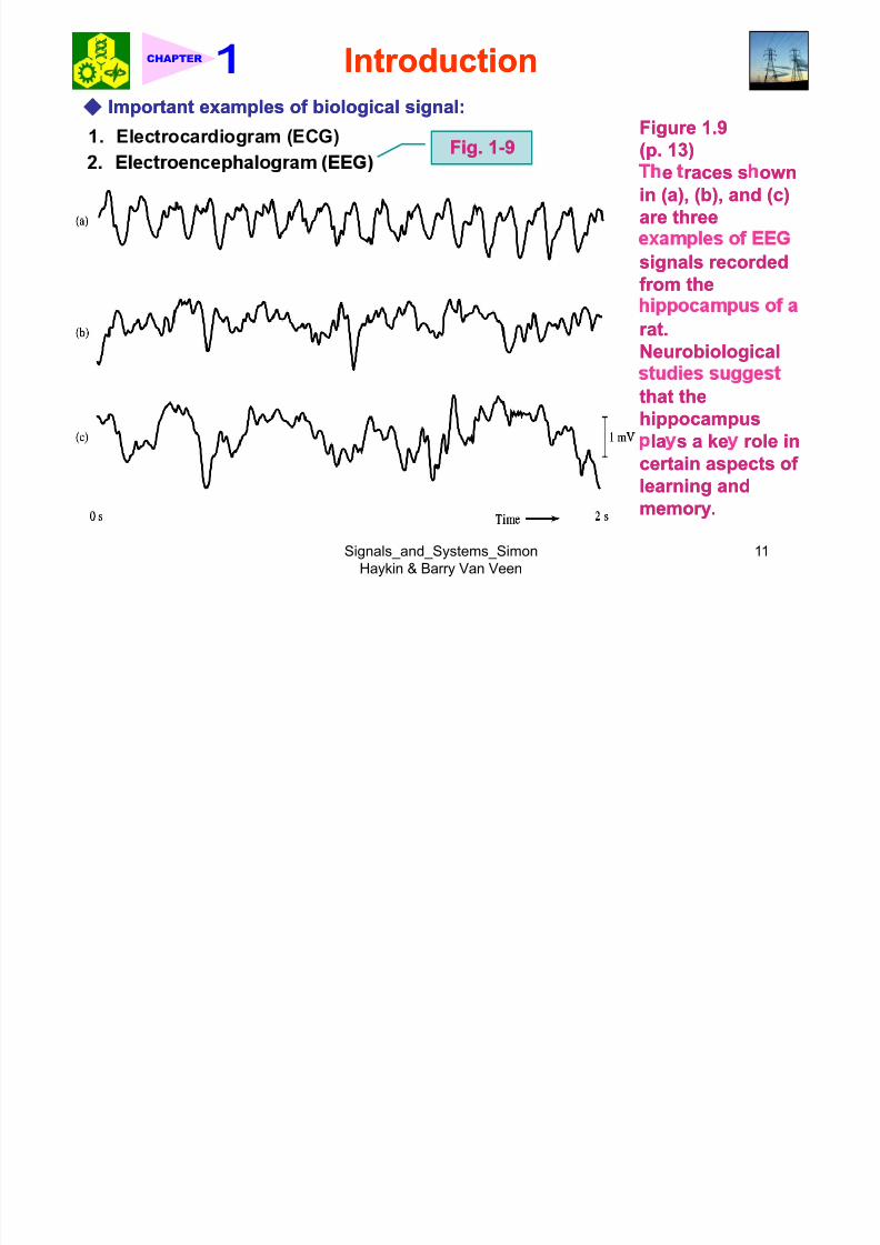
Important examples of biological signal:Important examples of biological signal:1. Electrocardiogram (ECG)
Fig.Fig. 11--99FigureFigure 11..99
(p.(p. 1313))
e races s owne races s own
in (a), (b), and (c)in (a), (b), and (c)
are threeare three
signals recordedsignals recorded
from thefrom the
rat.rat.NeurobiologicalNeurobiological
that thethat the
hippocampushippocampus
la s a ke role inla s a ke role incertain aspects ofcertain aspects of
learning andlearning and
memory.memory.
Signals_and_Systems_Simon
Haykin & Barry Van Veen
11

8/13/2019 Ch01 Introduction Compatibility Mode
http://slidepdf.com/reader/full/ch01-introduction-compatibility-mode 12/98
IntroductionIntroductionCHAPTER
★ Measurement artifacts:Measurement artifacts:11. Instrumental artifacts. Instrumental artifacts
22. Biolo ical artifacts. Biolo ical artifacts
33. Analysis artifacts. Analysis artifacts
★ 11..33..66 Auditory SystemAuditory System
Figure 1.10 (p. 14)
(a) In this diagram, the basilar
membrane in the cochlea is depicted
as if it were uncoiled and stretched
out flat; the “base” and “apex” refer
to the cochlea, but the remarks “stiff
reg on an ex e reg on re er o
the basilar membrane. (b) This
diagram illustrates the traveling ,
showing their envelopes induced by
incoming sound at three different
Signals_and_Systems_Simon
Haykin & Barry Van Veen
12
.
8/13/2019 Ch01 Introduction Compatibility Mode
http://slidepdf.com/reader/full/ch01-introduction-compatibility-mode 13/98
IntroductionIntroductionCHAPTER
★ The ear has three main parts:The ear has three main parts:1. Outer ear: collection of sound
.
Conveying the variations of the tympanic membrane (eardrum)
3. Inner ear: mechanical variations →→ electrochemical or neural signal
★ Basilar membrane: Traveling wave Fig.Fig. 11--1010..
★ 11..33..77 Analog Versus Digital Signal ProcessingAnalog Versus Digital Signal Processing
g a approac as wo a van ages over ana og approac :
1. Flexibility
2. Repeatability
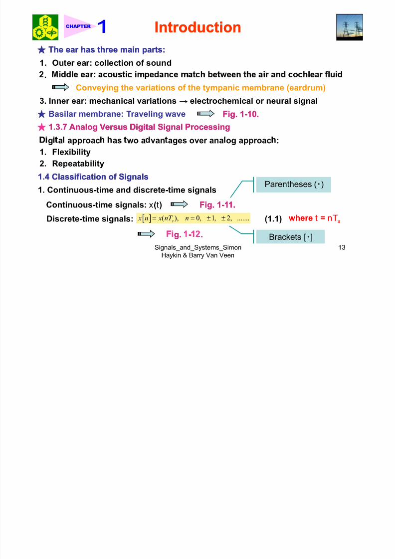
11..44 Classification of SignalsClassification of Signals
1. Continuous-time and discrete-time signalsParentheses (‧)
Continuous-time signals: x(t)
Discrete-time signals: [ ] ( ), 0, 1, 2, .......s
x n x nT n= = ± ± (1.1)
Fig.Fig. 11--1111..
where t = nTs
Signals_and_Systems_Simon
Haykin & Barry Van Veen
13
g.g. -- .. Brackets [‧]

8/13/2019 Ch01 Introduction Compatibility Mode
http://slidepdf.com/reader/full/ch01-introduction-compatibility-mode 14/98
IntroductionIntroductionCHAPTER
Figure 1.11 (p. 17)
Continuous-time signal.
gure . p.
(a) Continuous-time signal x(t). (b) Representation of x(t) as a
discrete-time signal x[n].
Signals_and_Systems_Simon
Haykin & Barry Van Veen
14

8/13/2019 Ch01 Introduction Compatibility Mode
http://slidepdf.com/reader/full/ch01-introduction-compatibility-mode 15/98
IntroductionIntroductionCHAPTER
2. Even and odd signals
Even signals: ( ) ( ) for all x t x t t − = (1.2)
− = − .
Antisymmetric about originExampleExample 11..11
Consider the signal
sin ,( )
t T t T
x t T
π ⎧ ⎞⎛ − ≤ ≤⎪ ⎜ ⎟= ⎝ ⎠⎨⎪ ,
Is the signal x(t) an even or an odd function of time?<Sol.><Sol.>
sint
T t T π ⎧ ⎞⎛ − − ≤ ≤
( )
0 , otherwise
x t T − =⎪⎩
sin ,=
0 , otherwise
T t T T
− − ≤ ≤⎪ ⎜ ⎟⎝ ⎠⎨
⎪⎩
Signals_and_Systems_Simon
Haykin & Barry Van Veen
15
= ( ) for all t x t −

8/13/2019 Ch01 Introduction Compatibility Mode
http://slidepdf.com/reader/full/ch01-introduction-compatibility-mode 16/98
IntroductionIntroductionCHAPTER
2( ) cost x t e t
−=
Even-odd decomposition of x(t):( ) ( ) ( )e o x t x t x t = +
ExampleExample 11..22Find the even and odd components
of the signale e x x− =
( ) ( )o o x t x t − = −
w ere2( ) cost
x t e t −=
<Sol.><Sol.>
( ) ( )
e o
e o
x t x t x t
x t x t
− = − + −
= − 2
cos
= cos( )t
x t e t
e t
− = −
(1.4)[ ]1 ( ) ( )2
e x x t x t = + −2 21
( ) ( cos cos )t t e x t e t e t
−= +Even component:
[ ]( ) ( )2
o x x t x t = − − (1.5)
cosh(2 ) cost t =
2 21( ) ( cos cos ) sinh(2 ) cost t
o x t e t e t t t −= − = −
Odd component:
Signals_and_Systems_Simon
Haykin & Barry Van Veen
16
8/13/2019 Ch01 Introduction Compatibility Mode
http://slidepdf.com/reader/full/ch01-introduction-compatibility-mode 17/98
IntroductionIntroductionCHAPTER
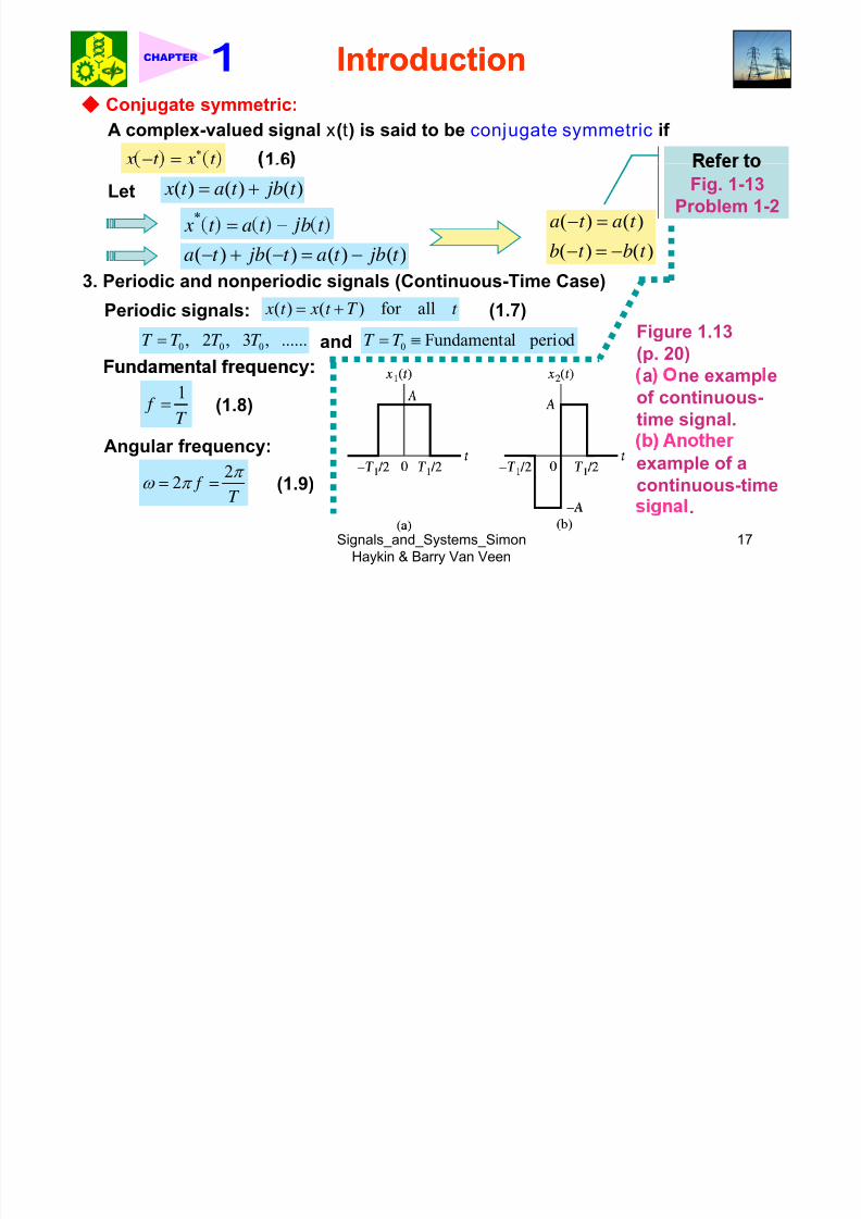
Conjugate symmetric:A complex-valued signal x(t) is said to be conjugate symmetric if
x t x t ∗− = 1.6
( ) ( ) ( ) x t a t jb t = +
* x t a t b t = −
Let
( ) ( )a t a t − =
Fig. 1-13
Problem 1-2
( ) ( ) ( ) ( )a t jb t a t jb t − + − = − ( ) ( )b t b t − = −
3. Periodic and nonperiodic signals (Continuous-Time Case)
Periodic signals: ( ) ( ) for all x t x t T t = + (1.7)
0 0 0, 2 , 3 , ......T T T T = 0 Fundamental period T T = ≡andFigure 1.13
(p. 20)
1 f
T =
(1.8)
a ne examp e
of continuous-
time signal.Angular frequency:
22 f
T
π ω π = = (1.9)
example of a
continuous-time
Signals_and_Systems_SimonHaykin & Barry Van Veen
17
.
8/13/2019 Ch01 Introduction Compatibility Mode
http://slidepdf.com/reader/full/ch01-introduction-compatibility-mode 18/98
IntroductionIntroductionCHAPTER
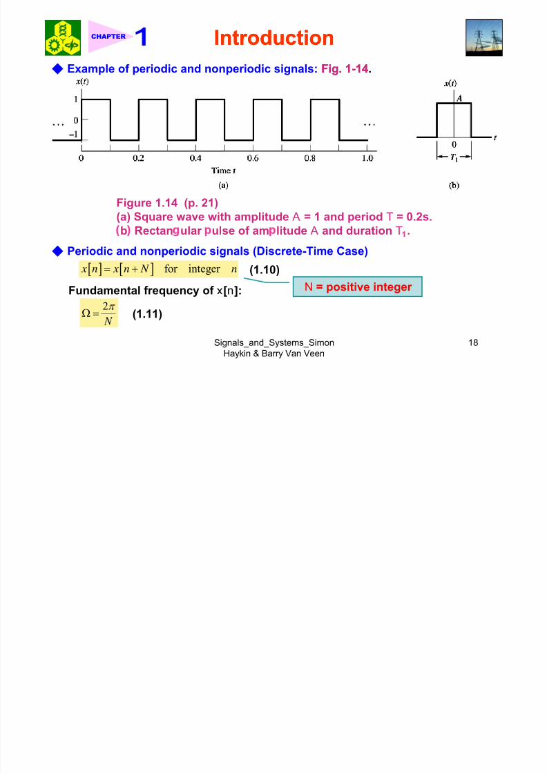
Example of periodic and nonperiodic signals: Fig.Fig. 11--1414.
Figure 1.14 (p. 21)(a) Square wave with amplitude A = 1 and period T = 0.2s.
b Rectan ular ulse of am litude A and duration T .
Periodic and nonperiodic signals (Discrete-Time Case)
[ ] [ ] for integer x n x n N n= + (1.10)N = positive integer Fundamental frequency of x[n]:
2π Ω = (1.11)
Signals_and_Systems_SimonHaykin & Barry Van Veen
18

8/13/2019 Ch01 Introduction Compatibility Mode
http://slidepdf.com/reader/full/ch01-introduction-compatibility-mode 19/98
IntroductionIntroductionCHAPTER
Figure 1.15 (p. 21)
Triangular wave alternative between –1 and +1 for Problem 1.3.
Fig.Fig. 11--1616 and Fig.and Fig. 11--1717.
Discrete-time square
wave alternative
between –1 and +1.
Signals_and_Systems_SimonHaykin & Barry Van Veen
19
8/13/2019 Ch01 Introduction Compatibility Mode
http://slidepdf.com/reader/full/ch01-introduction-compatibility-mode 20/98
IntroductionIntroductionCHAPTER
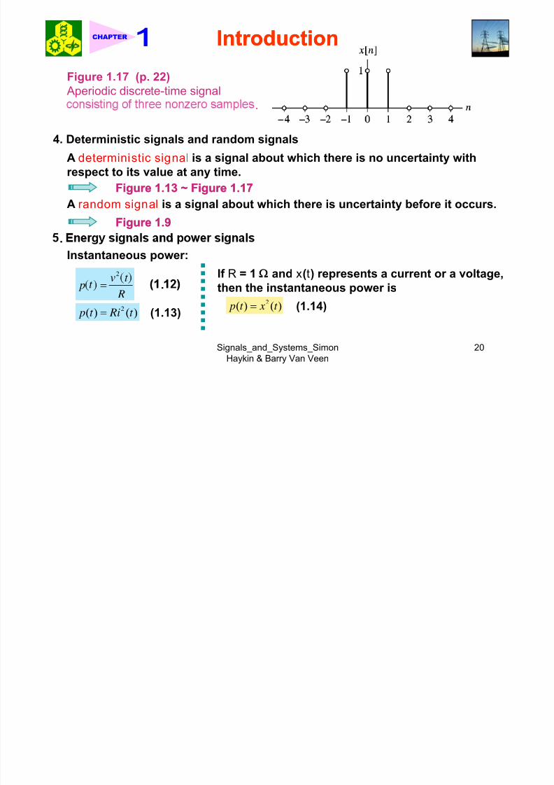
Figure 1.17 (p. 22)
Aperiodic discrete-time signal
.
4. Deterministic signals and random signalsA deterministic signal is a signal about which there is no uncertainty with
respect to its value at any time.
FigureFigure 11..1313 ~ Figure~ Figure 11..1717
A random signal is a signal about which there is uncertainty before it occurs.FigureFigure 11..99
.
Instantaneous power:
2v t If R = 1 Ω and x(t) represents a current or a voltage, p R
=
2( ) ( ) p t Ri t =
.
(1.13)
then the instantaneous power is2( ) ( ) p t x t = (1.14)
Signals_and_Systems_SimonHaykin & Barry Van Veen
20

8/13/2019 Ch01 Introduction Compatibility Mode
http://slidepdf.com/reader/full/ch01-introduction-compatibility-mode 21/98
IntroductionIntroductionCHAPTER
The total energy of the continuous-time signal x(t) is2 22lim ( ) ( )
T
T E x t dt x t dt ∞
− −∞∞= =∫ ∫ (1.15)
Discrete-time case:Total energy of x[n]:
2
Time-averaged, or average, power is
1 T
2[ ]n
E x n=−∞
= ∑ (1.18)
Avera e ower of x n :
2
m T T
x t t T
−→∞
=21
lim [ ]2
N
nn N
P x n N →∞
=−
= ∑(1.16)
For periodic signal, the time-averaged power is(1.19)
22
2
1 ( )T
T P x t dt T
−= ∫1
2
0
1 [ ] N
n
P x n N
−
== ∑(1.17)
.★ Energy signal:
If and only if the total energy of the signal satisfies the condition
★ Power signal:
If and only if the average power of the signal satisfies the condition
Signals_and_Systems_SimonHaykin & Barry Van Veen
21
∞

8/13/2019 Ch01 Introduction Compatibility Mode
http://slidepdf.com/reader/full/ch01-introduction-compatibility-mode 22/98
IntroductionIntroductionCHAPTER
11..55 Basic Operations on SignalsBasic Operations on Signals★ 11..55..11 Operations Performed on dependent VariablesOperations Performed on dependent Variables
Am litude scalin : x t t cx t = 1.21
c = scaling factor
Performed by amplifier Discrete-time case: x[n] [ ] [ ] y n cx n=
Addition:1 2 y x x= .
Discrete-time case: 1 2[ ] [ ] [ ] y n x n x n= +Multiplication:
1 2( ) ( ) ( ) y t x t x t =1 2[ ] [ ] [ ] y n x n x n=
(1.23)
x. mo u a on
Figure 1.18 (p. 26)
Inductor with current
i (t ), inducing voltage
Differentiation:
( ) ( )
d
y t x t = (1.24) Inductor:Inductor: ( ) ( )
d
v t L i t = (1.25)v (t ) across its
terminals.Integration:
t
=
Signals_and_Systems_SimonHaykin & Barry Van Veen
22
−∞.
8/13/2019 Ch01 Introduction Compatibility Mode
http://slidepdf.com/reader/full/ch01-introduction-compatibility-mode 23/98
IntroductionIntroductionCHAPTER
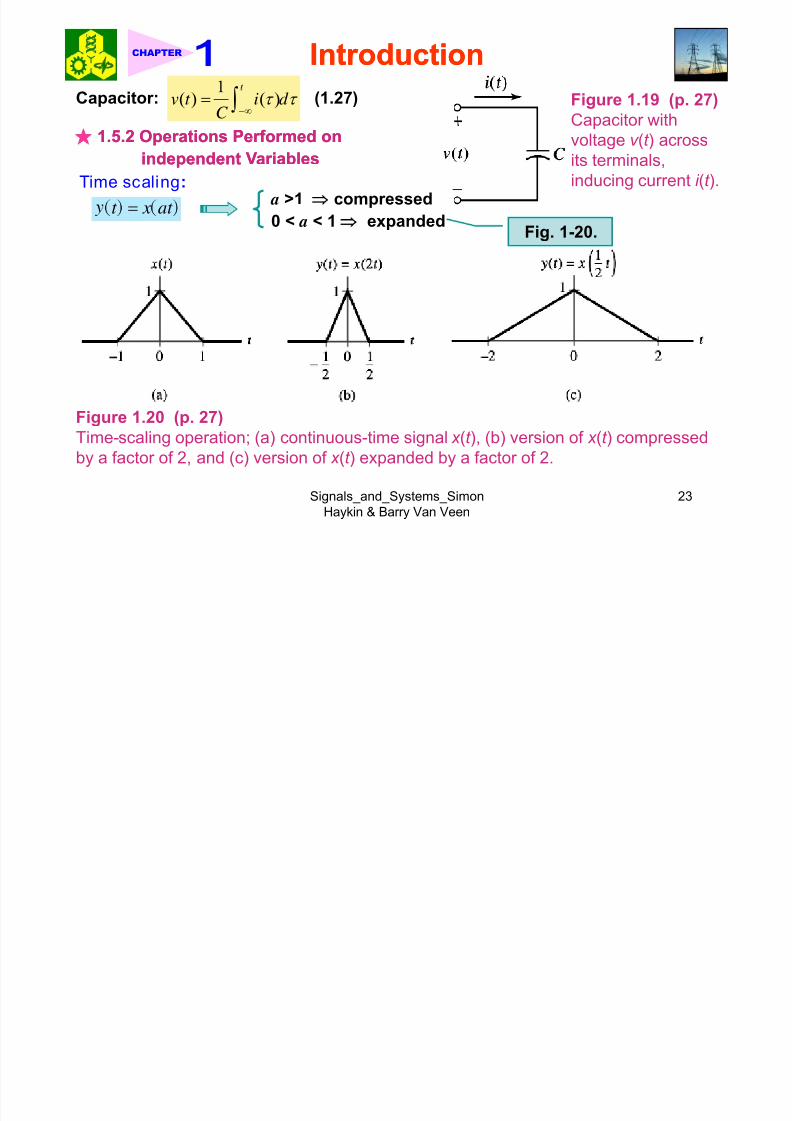
( ) ( )v t i d C τ τ −∞=Capacitor: (1.27) Figure 1.19 (p. 27)Capacitor with
voltage v (t ) across11..55..22 Operations Performed onOperations Performed on
its terminals,
inducing current i (t ).
independent Variablesindependent Variables
Time scaling:
t x at = a >1 ⇒ compressed0 < a < 1 ⇒ expanded
Fig. 1-20.
Figure 1.20 (p. 27)
Time-scaling operation; (a) continuous-time signal x (t ), (b) version of x (t ) compressed
by a factor of 2, and (c) version of x (t ) expanded by a factor of 2.
Signals_and_Systems_SimonHaykin & Barry Van Veen
23
8/13/2019 Ch01 Introduction Compatibility Mode
http://slidepdf.com/reader/full/ch01-introduction-compatibility-mode 24/98
IntroductionIntroductionCHAPTER
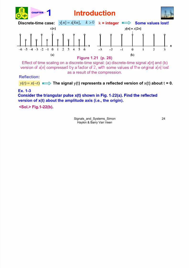
, y n x n= >Discrete-time case: k = integer Some values lost!
Figure 1.21 (p. 28)
Effect of time scaling on a discrete-time signal: (a) discrete-time signal x [n] and (b)
vers on o x n compresse y a ac or o , w some va ues o e or g na x n os
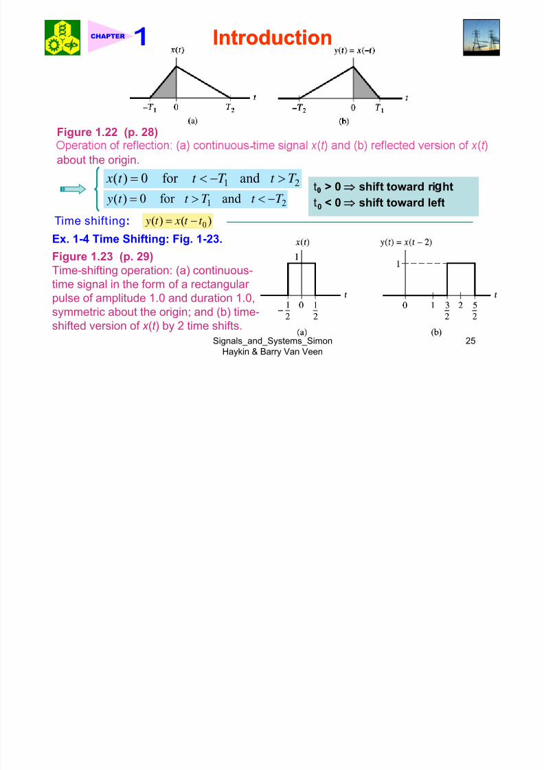
as a result of the compression.Reflection:
( ) ( ) y t x t = − The signal y(t) represents a reflected version of x(t) about t = 0.
Ex. 1-3
- version of x(t) about the amplitude axis (i.e., the origin).
<Sol.> Fig.<Sol.> Fig.11--2222(b)(b).
Signals_and_Systems_SimonHaykin & Barry Van Veen
24
8/13/2019 Ch01 Introduction Compatibility Mode
http://slidepdf.com/reader/full/ch01-introduction-compatibility-mode 25/98
IntroductionIntroductionCHAPTER
Figure 1.22 (p. 28) -
about the origin.
1 2( ) 0 for and x t t T t T = < − >t > 0 ⇒ shift toward ri ht
1 2( ) 0 for and y t t T t T = > < −Time shift ing: 0( ) ( ) y t x t t = −
⇒
t0 < 0 ⇒ shift toward left
Ex. 1-4 Time Shifting: Fig. 1-23.
Figure 1.23 (p. 29)
Time-shifting operation: (a) continuous-time signal in the form of a rectangular
pulse of amplitude 1.0 and duration 1.0,
symmetric about the origin; and (b) time-
Signals_and_Systems_SimonHaykin & Barry Van Veen
25
shifted version of x (t ) by 2 time shifts.
8/13/2019 Ch01 Introduction Compatibility Mode
http://slidepdf.com/reader/full/ch01-introduction-compatibility-mode 26/98

8/13/2019 Ch01 Introduction Compatibility Mode
http://slidepdf.com/reader/full/ch01-introduction-compatibility-mode 27/98
IntroductionIntroductionCHAPTER
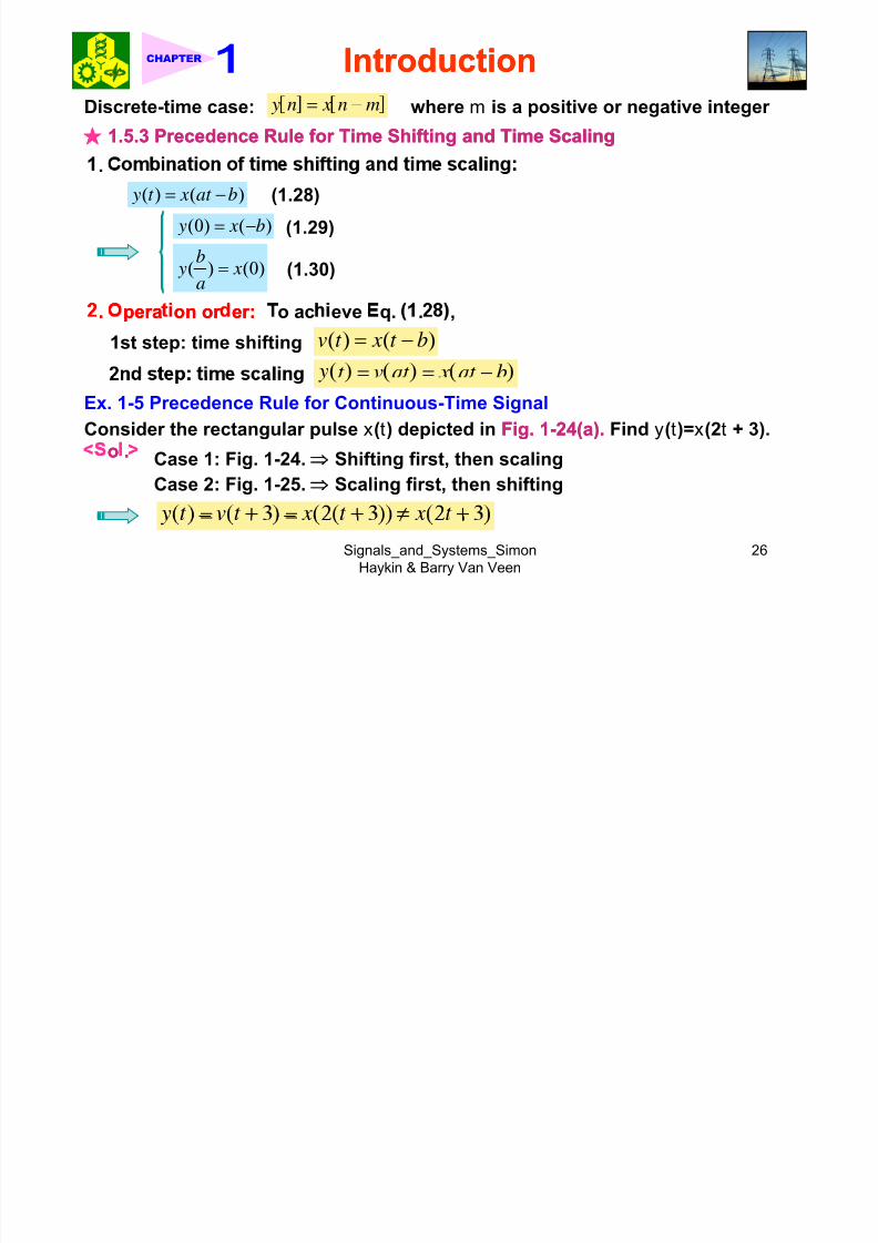
Figure 1.24 (p. 31)
The ro er order in which the o erations of time scalin and time shiftin
should be applied in the case of the continuous-time signal of Example 1.5.
(a) Rectangular pulse x (t ) of amplitude 1.0 and duration 2.0, symmetric
about the origin. (b) Intermediate pulse v (t ), representing a time-shiftedversion of x (t ). (c) Desired signal y (t ), resulting from the compression of v (t )
by a factor of 2.
Signals_and_Systems_SimonHaykin & Barry Van Veen
27

8/13/2019 Ch01 Introduction Compatibility Mode
http://slidepdf.com/reader/full/ch01-introduction-compatibility-mode 28/98
IntroductionIntroductionCHAPTER
Figure 1.25 (p. 31)
w y y u . .
(b) Time-scaled signal v (t ) = x (2t ). (c) Signal y (t ) obtained by shiftingv (t ) = x (2t ) by 3 time units, which yields y (t ) = x (2(t + 3)).
x. - rece ence u e or scre e- me gna
A discrete-time signal is defined by
1, 1,2n =⎧[ ] 1, 1, 2
0, 0 and | | 2
x n n
n n
= − = − −⎨⎪ = >⎩
Signals_and_Systems_SimonHaykin & Barry Van Veen
28
Find y[n] = x[2x + 3].

8/13/2019 Ch01 Introduction Compatibility Mode
http://slidepdf.com/reader/full/ch01-introduction-compatibility-mode 29/98
IntroductionIntroductionCHAPTER
<Sol.> See Fig.<Sol.> See Fig. 11--2727..
Figure 1.27 (p. 33)
The proper order of applying the operations of time scaling and time shifting for thecase of a discrete-time signal. (a) Discrete-time signal x [n], antisymmetric about the
origin. (b) Intermediate signal v (n) obtained by shifting x [n] to the left by 3 samples.
(c) Discrete-time signal y [n] resulting from the compression of v [n] by a factor of 2,
Signals_and_Systems_SimonHaykin & Barry Van Veen
29
as a result of which two samples of the original x [n], located at n = –2, +2, are lost.

8/13/2019 Ch01 Introduction Compatibility Mode
http://slidepdf.com/reader/full/ch01-introduction-compatibility-mode 30/98
IntroductionIntroductionCHAPTER
11..66 Elementary SignalsElementary Signals★ 11..66..11 Exponential SignalsExponential Signals ( ) a t
x t Be= (1.31)
a
1. Deca in ex onential for which < 0
2. Growing exponential, for which a > 0
Figure 1.28 (p. 34)
(a) Decaying exponential form of continuous-time signal. (b) Growing exponential
Signals_and_Systems_SimonHaykin & Barry Van Veen
30
orm o con nuous- me s gna .
8/13/2019 Ch01 Introduction Compatibility Mode
http://slidepdf.com/reader/full/ch01-introduction-compatibility-mode 31/98
IntroductionIntroductionCHAPTER
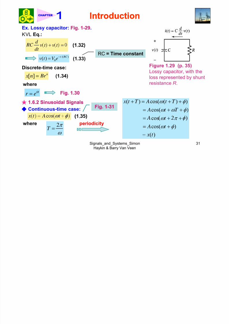
Ex. Lossy capacitor: Fig.Fig. 11--2929.
d
KVL Eq.:
v t v t dt
+ = .
/( )0( )
t RC
v t V e−
= (1.33)
RC = Time constant
Figure 1.29 (p. 35)
Lossy capacitor, with the
loss represented by shunt
Discrete-time case:
[ ] n x n Br = (1.34)
resistance R .
r eα =where
Fig.Fig. 11..3030
★ 11..66..22 Sinusoidal SignalsSinusoidal Signals ( ) cos( ( ) )
cos( )
x t T A t T
A t T
ω φ
ω ω φ
+ = + +
= + +Continuous-time case:Fig.Fig. 11--3131
2T
π
ω =
.
where cos
cos( )
t
A t
ω π
ω φ
= + +
= +periodicity
Signals_and_Systems_SimonHaykin & Barry Van Veen
31

8/13/2019 Ch01 Introduction Compatibility Mode
http://slidepdf.com/reader/full/ch01-introduction-compatibility-mode 32/98
IntroductionIntroductionCHAPTER
Figure 1.30 (p. 35)
a Deca in ex onential form of discrete-time si nal. b Growin exponential form of discrete-time signal.
Signals_and_Systems_SimonHaykin & Barry Van Veen
32
I d iI d i
8/13/2019 Ch01 Introduction Compatibility Mode
http://slidepdf.com/reader/full/ch01-introduction-compatibility-mode 33/98
IntroductionIntroductionCHAPTER
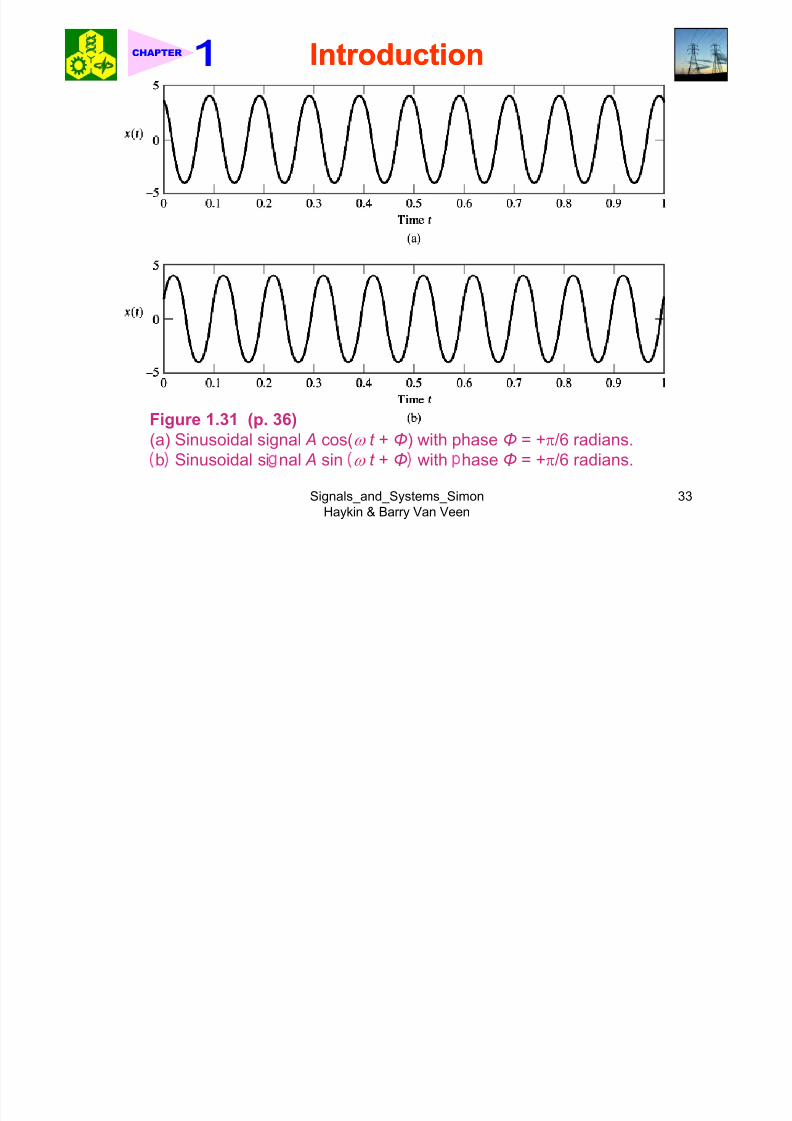
Figure 1.31 (p. 36)
(a) Sinusoidal signal A cos(ω t + Φ) with phase Φ = +π/6 radians.
b Sinusoidal si nal A sin ω t + Φ with hase Φ = +π/6 radians.
Signals_and_Systems_SimonHaykin & Barry Van Veen
33
I t d tiI t d ti

8/13/2019 Ch01 Introduction Compatibility Mode
http://slidepdf.com/reader/full/ch01-introduction-compatibility-mode 34/98
IntroductionIntroductionCHAPTER
Ex. Generation of a sinusoidal signal ⇒ Fig.Fig. 11--3232.Circuit Eq.:2d 2
0 LC v t v t dt
+ =
0 0( ) cos( ), 0v t V t t ω = ≥
(1.36)
(1.37)
Figure 1.32 (p. 37)
Parallel LC circuit,
assumin that the
where0
1
LC ω = (1.38)
Natural an ular fre uenc
inductor L and capacitorC are both ideal.
of oscillation of the circuit
Discrete-time case :
cos x n n= +
[ ] cos( ) x n N A n N φ + = Ω + Ω + (1.40)
(1.39)
Periodic condition:
2 N mπ Ω = radians/cycle, integer ,m
m N N
π Ω =or
- = φ= = --
(1.41)
Signals_and_Systems_SimonHaykin & Barry Van Veen
34
φ
I t d tiI t d ti

8/13/2019 Ch01 Introduction Compatibility Mode
http://slidepdf.com/reader/full/ch01-introduction-compatibility-mode 35/98
IntroductionIntroductionCHAPTER
Figure 1.33 (p. 38)
-
Signals_and_Systems_SimonHaykin & Barry Van Veen
35
.
I t d tiI t d ti

8/13/2019 Ch01 Introduction Compatibility Mode
http://slidepdf.com/reader/full/ch01-introduction-compatibility-mode 36/98
IntroductionIntroductionCHAPTER
Example 1.7 Discrete-Time Sinusoidal Signal
A pair of sinusoidal signals with a common angular frequency is defined by
sin 5 x n nπ = =and
(a) Both x1[n] and x2[n] are periodic. Find their common fundamental period.
(b) Express the composite sinusoidal signal1 2 y n x n x n= +
In the form y[n] = Acos(Ωn + φ), and evaluate the amplitude A and phase φ.
..
(a) Angular frequency of both x1[n] and x2[n]:
5 radians/c cleπ Ω = 2 2 2m m mπ π = = =
5 5π ΩThis can be only for m = 5, 10, 15, …, which results in N = 2, 4, 6, …
cos( ) cos( )cos( ) sin( )sin( )n A n A nφ φ φ Ω + = Ω − Ω
x n + x n with the above e uation to obtain thatLet Ω = 5π then com are
Signals_and_Systems_SimonHaykin & Barry Van Veen
36
Introd ctionIntrod ction

8/13/2019 Ch01 Introduction Compatibility Mode
http://slidepdf.com/reader/full/ch01-introduction-compatibility-mode 37/98
IntroductionIntroductionCHAPTER
sin( ) 1 and cos( ) 3 A Aφ φ = − =1sin( ) amplitude of [ ] 1
tan x nφ −
= = = = π
2cos( ) amplitude of [ ] 3 x nφ
sin( ) 1 A φ = −
π
( )1
2sin / 6
Aπ
−= =
−Accordingly, we may express y[n] as
[ ] 2cos 56
y n n π π ⎛ ⎞= −⎜ ⎟⎝ ⎠★ 11..66..33 Relation Between Sinusoidal and Complex Exponential SignalsRelation Between Sinusoidal and Complex Exponential Signals
1. Euler’s identity: cos sin je j
θ θ θ = + (1.41) j t
Be ω
e=
j t ω =
( )
j t
e e
Ae φ ω +
=
=( ) cos( ) x t A t ω φ = + (1.35)
Signals_and_Systems_SimonHaykin & Barry Van Veen
37
.cos( ) sin( )t jA t ω φ ω φ = + + +
IntroductionIntroductionCHAPTER
8/13/2019 Ch01 Introduction Compatibility Mode
http://slidepdf.com/reader/full/ch01-introduction-compatibility-mode 38/98
IntroductionIntroductionCHAPTER
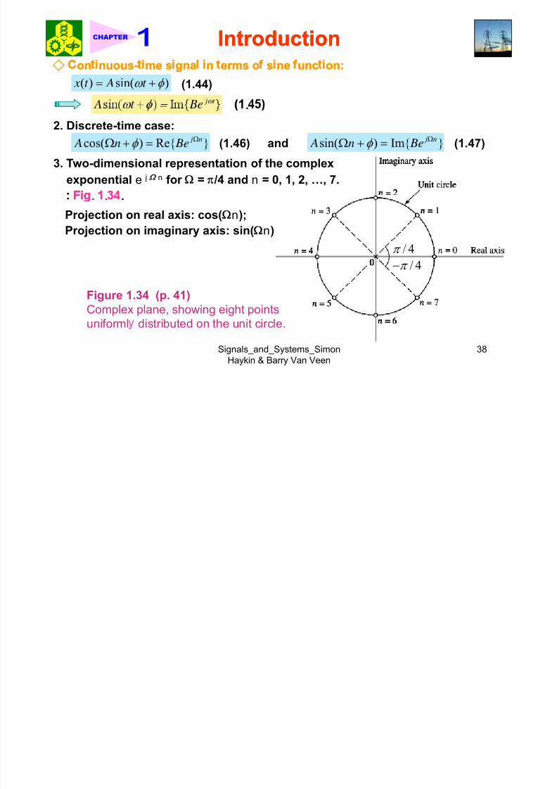
on nuouson nuous-- me s gna n erms o s ne unc on:me s gna n erms o s ne unc on:
( ) sin( ) x t A t ω φ = + (1.44)
j t ω = .
2. Discrete-time case:
cos( ) Re{ } j n
A n Beφ Ω
Ω + = (1.46) (1.47)and sin( ) Im{ } j n
A n Beφ Ω
Ω + =3. Two-dimensional representation of the complex
exponential e j n for Ω = π /4 and n = 0, 1, 2, …, 7.
.. .. .
Projection on real axis: cos(Ωn);Projection on imaginary axis: sin(Ωn)
/ 4π
/ 4π −
Figure 1.34 (p. 41)
Complex plane, showing eight points
uniforml distributed on the unit circle.
Signals_and_Systems_SimonHaykin & Barry Van Veen
38
IntroductionIntroductionCHAPTER
8/13/2019 Ch01 Introduction Compatibility Mode
http://slidepdf.com/reader/full/ch01-introduction-compatibility-mode 39/98
IntroductionIntroductionCHAPTER
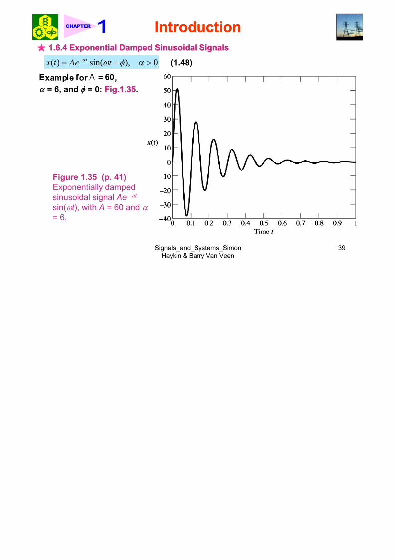
★ 11..66..44 Exponential Damped Sinusoidal SignalsExponential Damped Sinusoidal Signals
( ) sin( ), 0t x t Ae t
α ω φ α −= + > (1.48)
xamp e or = ,
α = 6, and φ = 0: Fig.Fig.11..3535.
Figure 1.35 (p. 41)
Exponentially damped
sinusoidal signal Ae−at
sin(ω t ), with A = 60 and α
= 6.
Signals_and_Systems_SimonHaykin & Barry Van Veen
39
IntroductionIntroductionCHAPTER

8/13/2019 Ch01 Introduction Compatibility Mode
http://slidepdf.com/reader/full/ch01-introduction-compatibility-mode 40/98
IntroductionIntroductionCHAPTER
( )v d L τ τ −∞Ex. Generation of an exponential damped sinusoidal signal
⇒ Fig.Fig. 11--3636.
1 1 t d rcu q.: v v v
dt R Lτ τ
−∞= .
/(2 )
0 0( ) cos( ) 0
t CR
v t V e t t ω
−
= ≥ (1.50)
Figure 1.36 (p. 42)0 2 2
1 1
4 LC C Rω = −where (1.51) /(4 ) R L C >
Parallel LRC, circuit, with
inductor L, capacitor C ,and resistor R all
ompar ng q. . an . , we ave
0 0, 1/(2 ), , and / 2 A V CRα ω ω φ π = = = = -
assume o e ea .
[ ] sin[ ]n x n Br n φ = Ω + (1.52)
★11..66..55 Step FunctionStep Function Figure 1.37 (p. 43)
x [n]
Discrete-time case:
{1, 00, 0[ ] n
nu n ≥
<= (1.53)
Discrete-time version
of step function of unit
amplitude. n
1
Signals_and_Systems_SimonHaykin & Barry Van Veen
40
Fig.Fig. 11--3737.. −−−
IntroductionIntroductionCHAPTER

8/13/2019 Ch01 Introduction Compatibility Mode
http://slidepdf.com/reader/full/ch01-introduction-compatibility-mode 41/98
IntroductionIntroductionCHAPTER
1, 0( )
t u t
>=
Continuous-time case:
(1.54)
Figure 1.38 (p. 44)
Continuous-time
version of the unit-step, unc on o un
amplitude.
Example 1.8 Rectangular PulseConsider the rectangular pulse x(t) shown in Fig.Fig. 11..3939 (a).(a). This pulse has an
amplitude A and duration of 1 second. Express x(t) as a weighted sum of two
step functions.
<Sol.><Sol.>
, 0 0.5( )0, 0.5 A t x t
t ⎧ ≤ <= ⎨ >⎩1. Rectangular pulse x(t): (1.55)
1 1( )
2 2 x t Au t Au t
⎞⎛ ⎛ = + − −⎜ ⎟ ⎜ ⎟⎝ ⎝ ⎠
(1.56)
Example 1.9 RC Circuit
Find the response v(t) of RC circuit shown in Fig.Fig. 11..4040 (a).(a).
<Sol.><Sol.>
Signals_and_Systems_SimonHaykin & Barry Van Veen
41
IntroductionIntroductionCHAPTER

8/13/2019 Ch01 Introduction Compatibility Mode
http://slidepdf.com/reader/full/ch01-introduction-compatibility-mode 42/98
IntroductionIntroductionCHAPTER
Figure 1.39 (p. 44)
(a) Rectangular pulse x (t ) of amplitude A and duration of 1 s, symmetric about the
origin. (b) Representation of x (t ) as the difference of two step functions of amplitude A, with one step function shifted to the left by ½ and the other shifted to the right by
½; the two shifted signals are denoted by x 1(t ) and x 2(t ), respectively. Note that x (t )
= x (t ) – x (t ).
Signals_and_Systems_SimonHaykin & Barry Van Veen
42
IntroductionIntroductionCHAPTER

8/13/2019 Ch01 Introduction Compatibility Mode
http://slidepdf.com/reader/full/ch01-introduction-compatibility-mode 43/98
IntroductionIntroduction
Figure 1.40 (p. 45)
,
the voltage source. (b) Equivalent circuit, using a step function to replace theaction of the switch.
1. Initial value: (0) 0v =
0( )v V ∞ =2. Final value:
( )/( )0( ) 1 ( )t RC
v t V e u t −= − (1.57)
. omp e e so u on:
Signals_and_Systems_SimonHaykin & Barry Van Veen
43
IntroductionIntroductionCHAPTER
8/13/2019 Ch01 Introduction Compatibility Mode
http://slidepdf.com/reader/full/ch01-introduction-compatibility-mode 44/98
IntroductionIntroduction
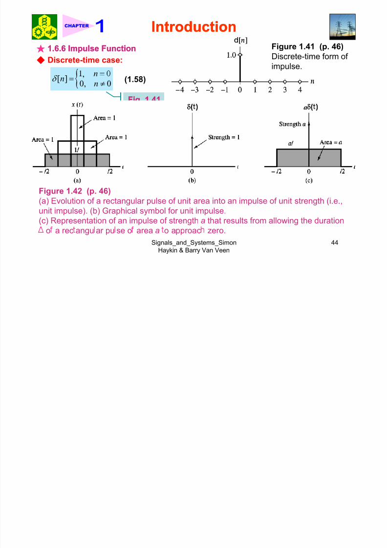
★11..66..66 Impulse FunctionImpulse Function
Figure 1.41 (p. 46)
Discrete-time form of
impulse. Discrete-time case:
,[ ]
0, 0n
nδ =
≠ (1.58)
Fig.Fig. 11..4141δ δ
Figure 1.41 (p. 46)
Discrete-time form of impulse.
δ aδ
Figure 1.42 (p. 46)
(a) Evolution of a rectangular pulse of unit area into an impulse of unit strength (i.e.,
unit impulse). (b) Graphical symbol for unit impulse.
(c) Representation of an impulse of strength a that results from allowing the duration
Signals_and_Systems_SimonHaykin & Barry Van Veen
44
o a rec angu ar pu se o area a o approac zero.
IntroductionIntroductionCHAPTER
8/13/2019 Ch01 Introduction Compatibility Mode
http://slidepdf.com/reader/full/ch01-introduction-compatibility-mode 45/98
IntroductionIntroduction
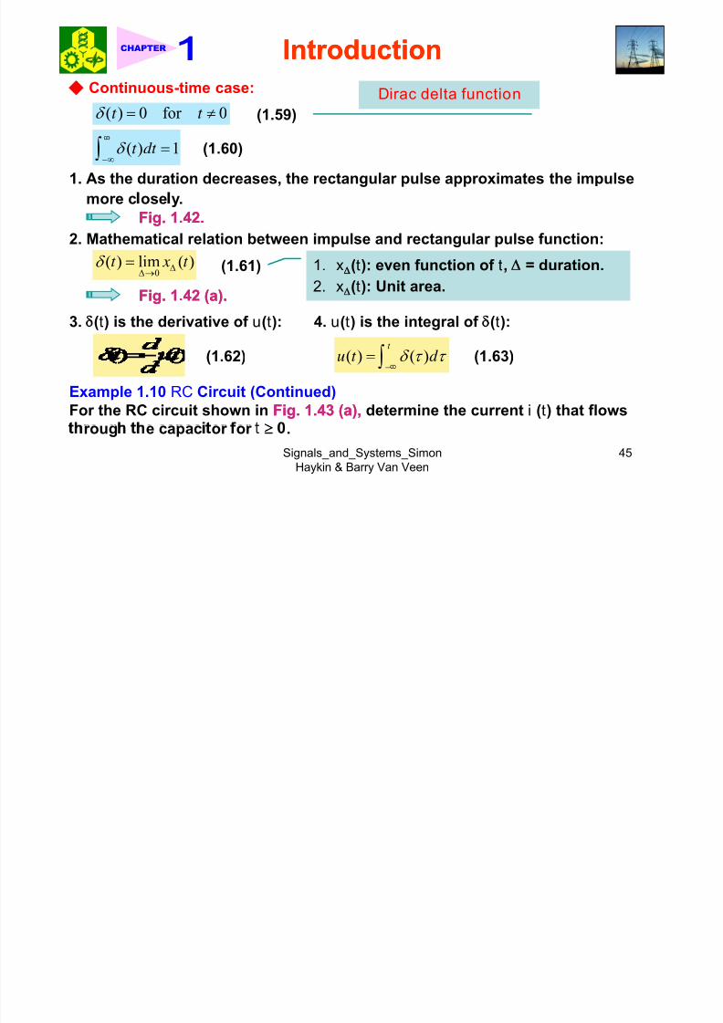
Continuous-time case:
( ) 0 for 0t t δ = ≠ (1.59)Dirac delta function
( ) 1t dt δ −∞
= (1.60)
1. As the duration decreases, the rectangular pulse approximates the impulse
more c ose y.
Fig.Fig. 11..4242..
2. Mathematical relation between impulse and rectangular pulse function:
0
( ) lim ( )t x t δ Δ
Δ→
= (1.61) 1. x (t): even function of t, = duration.
2. x (t): Unit area.Fig.Fig. 11..4242 (a).(a).
3. δ(t) is the derivative of u(t):
(1.62)
4. u(t) is the integral of δ(t):
( ) ( )t
u t d δ τ τ −
= (1.63)
Example 1.10 RC Circuit (Continued)
For the RC circuit shown in Fig.Fig. 11..4343 (a),(a), determine the current i (t) that flows
≥
Signals_and_Systems_SimonHaykin & Barry Van Veen
45
roug e capac or or ≥ .
IntroductionIntroductionCHAPTER

8/13/2019 Ch01 Introduction Compatibility Mode
http://slidepdf.com/reader/full/ch01-introduction-compatibility-mode 46/98
IntroductionIntroduction
<Sol.><Sol.>
Fi ure 1.43 . 47
(a) Series circuit consisting of a capacitor, a dc voltage source, and a switch; the
switch is closed at time t = 0. (b) Equivalent circuit, replacing the action of the
switch with a step function u(t ).
1. Voltage across the capacitor:
2. Current flowing through capacitor:
( )( )
dv t i t C = 0 0
( )( ) ( )
du t i t CV CV t δ = =
Signals_and_Systems_SimonHaykin & Barry Van Veen
46
t t
IntroductionIntroductionCHAPTER

8/13/2019 Ch01 Introduction Compatibility Mode
http://slidepdf.com/reader/full/ch01-introduction-compatibility-mode 47/98
IntroductionIntroduction
Properties of impulse function:
1. Even function: ( ) ( )t t δ δ − = (1.64)
2. Siftin ro ert :0
1lim ( ) ( ) x at t a
δ ΔΔ→= (1.68)
0 0( ) ( ) ( ) x t t t dt x t δ ∞
−∞− =∫ (1.65)
Ex. RLC circuit driven by impulsive
source: Fig.Fig. 11..4545..
. -
1( ) ( ), 0at t a
aδ δ = > (1.66)
001 I +
or g.g. .. aa , e vo age across
the capacitor at time t = 0+ is
<p.f.><p.f.> 0 00C C − .
Fig.Fig. 11..4444
1. Rectangular pulse approximation:
0ma x aΔΔ→
= (1.67)
2. Unit area pulse: Fig.Fig. 11..4444(a).(a).
me sca ng: g.g. .. ..
Area = 1/ a
Restoring unit area ax ( at)
Signals_and_Systems_SimonHaykin & Barry Van Veen
47
IntroductionIntroductionCHAPTER

8/13/2019 Ch01 Introduction Compatibility Mode
http://slidepdf.com/reader/full/ch01-introduction-compatibility-mode 48/98
IntroductionIntroduction
Figure 1.44 (p. 48)
- .
pulse x ∆
(t ) of amplitude 1/ ∆
and duration ∆
, symmetric about the origin. (b) Pulse x ∆
(t )compressed by factor a. (c) Amplitude scaling of the compressed pulse, restoring it to
unit area.
Figure 1.45 (p. 49)
(a) Parallel LRC circuit
r ven y an mpu s ve
current signal. (b) Series
LRC circuit driven by an
Signals_and_Systems_SimonHaykin & Barry Van Veen
48
u v v .
IntroductionIntroductionCHAPTER
8/13/2019 Ch01 Introduction Compatibility Mode
http://slidepdf.com/reader/full/ch01-introduction-compatibility-mode 49/98
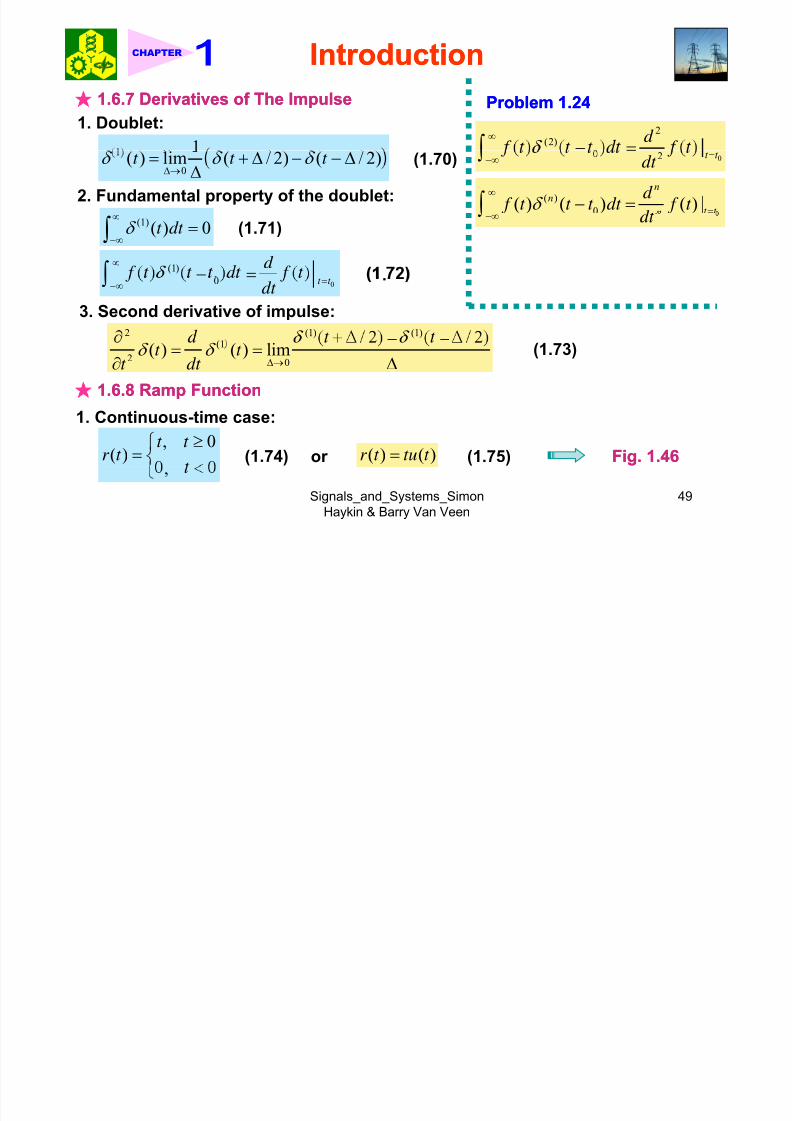
★ 11..66..77 Derivatives of The ImpulseDerivatives of The Impulse
1. Doublet:
1
ProblemProblem 11..24242
(2) d ∞− =
0( ) lim ( / 2) ( / 2)t t t δ δ δ
Δ→= + Δ − − Δ
Δ(1.70)
2. Fundamental property of the doublet:
02 t t dt
=−∞
( )0( ) ( ) ( ) |
nn
t t n
d
f t t t dt f t δ
∞
=− =(1)( ) 0t dt δ ∞
−∞=∫ (1.71)
(1) d ∞− =
−∞
00 t t dt
=−∞.
2 (1) (1)− −
3. Second derivative of impulse:
(1
2 0( ) ( ) limt t
t dt δ δ
Δ→= =
∂ Δ(1.73)
★ 11..66..88 Ramp FunctionRamp Function
1. Continuous-time case:
, 0( )
t t r t
≥⎧= ⎨ (1.74) ( ) ( )r t tu t =or (1.75) Fig.Fig. 11..4646
Signals_and_Systems_SimonHaykin & Barry Van Veen
49
,
IntroductionIntroductionCHAPTER

8/13/2019 Ch01 Introduction Compatibility Mode
http://slidepdf.com/reader/full/ch01-introduction-compatibility-mode 50/98
2. Discrete-time case:
, 0[ ]
n nr n
≥⎧= ⎨ (1.76)
Figure 1.46 (p. 51)
Ramp function of unit
slope.,
or
[ ] [ ]r n nu n= (1.77)
Figure 1.47 (p. 52)
-
x [n]Fig.Fig. 11..4747..
Example 1.11 Parallel Circuit
of the ramp function.ons er e para e c rcu o
Fig. 1-48 (a) involving a dccurrent source I0 and an
n1 2 3 40−1−2−3
n a y unc arge capac or .
The switch across the capacitor is suddenly
opened at time t = 0. Determine the current i(t)
ow ng roug e capac or an evoltage v(t) across it for t ≥ 0.
<Sol.><Sol.>
Signals_and_Systems_SimonHaykin & Barry Van Veen
50
. apac or curren : 0u=
IntroductionIntroductionCHAPTER

8/13/2019 Ch01 Introduction Compatibility Mode
http://slidepdf.com/reader/full/ch01-introduction-compatibility-mode 51/98
2. Capacitor voltage:
1( ) ( )
t
v t i d τ τ −∞
= ∫Figure 1.48 (p. 52)
(a) Parallel circuit
consisting of a
0
1( ) ( )
t
v t I u d τ τ −∞
=
∫
current source,
switch, and
capacitor, the
0 for 0
t
I
<⎧⎪
=
capacitor is initially
assumed to be
uncharged, and the
0
ort t
C I
>⎪⎩
sw c s opene a
time t = 0. (b)Equivalent circuit
0
C
I
r t =
action of opening
the switch with the
C .
Signals_and_Systems_SimonHaykin & Barry Van Veen
51
IntroductionIntroductionCHAPTER

8/13/2019 Ch01 Introduction Compatibility Mode
http://slidepdf.com/reader/full/ch01-introduction-compatibility-mode 52/98
11..77 Systems Viewed as Interconnections of OperationsSystems Viewed as Interconnections of Operations
A system may be viewed as an interconnection of operationsinterconnection of operations that transforms an
input signal into an output signal with properties different from those of the
input signal.
1. Continuous-time case:
2. Discrete-time case:
.
[ ] { [ ]} y n H x n= (1.79) Figure 1.49 (p. 53)
Block diagram representation of operator H for (a)
continuous time and (b) discrete time.Fig.Fig. 11--4949 (a) and (b).(a) and (b).Example 1.12 Moving-average system
Consider a discrete-time system whose output signal y[n] is the average of the
three most recent values of the input signal x[n], that is
[ ] ( [ ] [ 1] [ 2])3
y n x n x n x n= + − + −
Formulate the operator H for this system; hence, develop a block diagram
Signals_and_Systems_SimonHaykin & Barry Van Veen
52
representation for it.
IntroductionIntroductionCHAPTER

8/13/2019 Ch01 Introduction Compatibility Mode
http://slidepdf.com/reader/full/ch01-introduction-compatibility-mode 53/98
<Sol.><Sol.> 1. Discrete-time-shift operator Sk: Fig.Fig. 11..5050.
Shifts the input x[n] by k time units to
roduce an out ut e ual to x n k .
21=
Figure 1.50 (p. 54)
Discrete-time-shift operator
Sk o eratin on the discrete-
2. Overall operator HH for the moving-average
system:
3 time signal x [n] to produce
x [n – k ].
.. ..
Fig.Fig. 11--5151 (a): cascade form; Fig.(a): cascade form; Fig. 11--5151 (b): parallel(b): parallel
form.form.
11..88 Properties of SystemsProperties of Systems★ 11..88..11 StabilityStability
. - , -
only if every bounded input results in a bounded output.
2. The operator HH is BIBO stable if the output signal y(t) satisfies the condition
( ) for all y y t M t ≤ < ∞ (1.80)
whenever the input signals x(t) satisfy the condition Both Mx and My
represent some finite
Signals_and_Systems_SimonHaykin & Barry Van Veen
53
x . positive number

8/13/2019 Ch01 Introduction Compatibility Mode
http://slidepdf.com/reader/full/ch01-introduction-compatibility-mode 54/98
IntroductionIntroductionCHAPTER

8/13/2019 Ch01 Introduction Compatibility Mode
http://slidepdf.com/reader/full/ch01-introduction-compatibility-mode 55/98
One famous example of an unstableOne famous example of an unstablesystem:system:
. .
Dramatic photographs showing the
collapse of the Tacoma Narrows
, .(a) Photograph showing the twisting
motion of the bridge’s center span just
.
(b) A few minutes after the first piece of
concrete fell, this second photograph
shows a 600-ft section of the brid e
breaking out of the suspension span and
turning upside down as it crashed in Puget
Sound, Washin ton. Note the car in thetop right-hand corner of the photograph.
(Courtesy of the Smithsonian Institution.)
Signals_and_Systems_SimonHaykin & Barry Van Veen 55
IntroductionIntroductionCHAPTER

8/13/2019 Ch01 Introduction Compatibility Mode
http://slidepdf.com/reader/full/ch01-introduction-compatibility-mode 56/98
Example 1.13 Moving-average system (continued)
Show that the moving-average system described in Example 1.12 is BIBO stable.
<p.f.><p.f.>
1. Assume that: [ ] for all x x n M n≤ < ∞
2. Input-output relation:
( )1
[ ] [ ] [ 1] [ 2]3
y n x n x n x n= + − + −
[ ] [ ] [ 1] [ 2]3 y n x n x n x n= + − + −
[ ] [ 1] [ 2]3
1
x n x n x n≤ + − + − The movingThe moving--averageaverage
system is stable.system is stable.
3
x x x
x M =
Signals_and_Systems_SimonHaykin & Barry Van Veen 56
IntroductionIntroductionCHAPTER

8/13/2019 Ch01 Introduction Compatibility Mode
http://slidepdf.com/reader/full/ch01-introduction-compatibility-mode 57/98
Example 1.14 Unstable system
Consider a discrete-time system whose input-output relation is defined by
n
where r > 1. Show that this system is unstable.
<p.f.><p.f.>1. Assume that: [ ] for all x x n M n≤ < ∞
2. We find that
[ ] [ ] [ ] y n r x n r x n= = .
With r > 1, the multiplying factor r n diverges for increasing n.
The system is unstable.The system is unstable.
★ 11..88..22 MemoryMemory
sys em s sa o possess memory s ou pu s gna epen s on pas orfuture values of the input signal.
A system is said to possess memoryless if its output signal depends only on
Signals_and_Systems_SimonHaykin & Barry Van Veen 57
e presen va ues o e npu s gna .
IntroductionIntroductionCHAPTER

8/13/2019 Ch01 Introduction Compatibility Mode
http://slidepdf.com/reader/full/ch01-introduction-compatibility-mode 58/98
Ex.: Resistor 1
( ) ( )i t v t R= Memoryless !
Ex.: Inductor ( ) ( )t
i t v d L
τ τ −∞
= ∫ Memory !
Ex.: Movin -avera e s stem
1[ ] ( [ ] [ 1] [ 2])
3 y n x n x n x n= + − + − Memory !
Ex.: A system described by the input-output relation
2[ ] [ ] y n x n= Memoryless !
★ 11..88..33 CausalityCausality
A system is said to be causal if its present value of the output signal depends
on y on e presen or pas va ues o e npu s gna .A system is said to be noncausal if its output signal depends on one or more
future values of the input signal.
Signals_and_Systems_SimonHaykin & Barry Van Veen 58
IntroductionIntroductionCHAPTER

8/13/2019 Ch01 Introduction Compatibility Mode
http://slidepdf.com/reader/full/ch01-introduction-compatibility-mode 59/98
Ex.: Moving-average system
11 2n x n x n x n= + − + − Causal !
Ex.: Moving-average system
[ ] ( [ 1] [ ] [ 1])3
y n x n x n x n= + + + − Noncausal !
♣ A causal s stem must be ca able of o eratin in real timereal time.
★11..88..44 InvertibilityInvertibility
A system is said to be invertible if the
from the output.Figure 1.54 (p. 59)
The notion of system invertibility. The1. Continuous-time system: Fig.Fig. 11..5454.
second operator H inv is the inverse of the
first operator H . Hence, the input x (t ) is
passed through the cascade correction
x(t) = input; y(t) = output
H = first system operator;
H inv = second system operator
Signals_and_Systems_SimonHaykin & Barry Van Veen 59
o an nv comp e e y unc ange .
IntroductionIntroductionCHAPTER

8/13/2019 Ch01 Introduction Compatibility Mode
http://slidepdf.com/reader/full/ch01-introduction-compatibility-mode 60/98
2. Output of the second system:
{ } { }{ } { }( ) ( ) ( )inv inv inv H y t H H x t H H x t = = H
inv
= inverseoperator
3. Condition for invertible system:
inv H H I = (1.82)I = identity operator
.
Consider the time-shift system described by the input-output relation
0
0( ) ( ) ( )t y t x t t S x t = − =
where the operator S t0 represents a time shift of t0
seconds. Find the inverse of
this system.
<Sol.><Sol.>
1. Inverse operator S t 0:
0 0 0 0 0{ ( )} { { ( )}} { ( )}t t t t t
S y t S S x t S S x t − − −= =
2. Invertibility condition:
0 0t t S S I
− = 0t S
− ≡ Time shift of t0
Signals_and_Systems_SimonHaykin & Barry Van Veen 60
IntroductionIntroductionCHAPTER
8/13/2019 Ch01 Introduction Compatibility Mode
http://slidepdf.com/reader/full/ch01-introduction-compatibility-mode 61/98
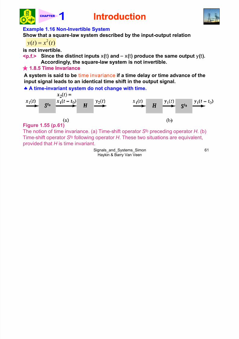
Example 1.16 Non-Invertible System
Show that a square-law system described by the input-output relation2( ) ( ) y t x t =
is not invertible.
<p.f.><p.f.> Since the distinct inputs x(t) and x(t) produce the same output y(t).
Accordingly, the square-law system is not invertible.★ 11..88..55 Time InvarianceTime Invariance
A system is said to be time invariance if a time delay or time advance of the
input signal leads to an identical time shift in the output signal.
♣ A time-invariant system do not change with time.
Figure 1.55 (p.61)
The notion of time invariance. (a) Time-shift operator St 0 preceding operator H . (b)
Time-shift operator St 0 following operator H . These two situations are equivalent,
Signals_and_Systems_SimonHaykin & Barry Van Veen 61
provided that H is time invariant.
IntroductionIntroductionCHAPTER

8/13/2019 Ch01 Introduction Compatibility Mode
http://slidepdf.com/reader/full/ch01-introduction-compatibility-mode 62/98
1. Continuous-time system:
1 1( ) { ( )} y t H x t =. 1 0
0
2 1 0 1( ) ( ) { ( )}t x t x t t S x t = − = S t 0 = operator of a time shift equal to t0
. u pu o sys em :
0
2 1 0( ) { ( )}t
y t H x t t = −
0
1
1{ ( )}t
HS x t =
.
4. For Fi .Fi . 11--5555 bb the out ut of s stem H is t t :
0
0
1 0 1( ) { ( )}t
t
y t t S y t
S H x t
− =
= 1.840
1{ ( )}t S H x t =
5. Condition for time-invariant system: 0 0t t HS S H = (1.85)
Signals_and_Systems_SimonHaykin & Barry Van Veen 62
IntroductionIntroductionCHAPTER
t = i t

8/13/2019 Ch01 Introduction Compatibility Mode
http://slidepdf.com/reader/full/ch01-introduction-compatibility-mode 63/98
t i tExample 1.17 Inductor
x (t) = v(t)
The inductor shown in figure is described
by the input-output relation: 1 t
1 1 y t x L
τ τ −∞
=
where L is the inductance. Show that the inductor so described is time invariant.
..
1. Let x1(t) x1(t t0) Response y2(t) of the inductor to x1(t t0) is
1 t
2 1 0 y x
L
τ τ −∞
= −
2. Let y1(t t0) = the original output of the inductor, shifted by t0 seconds:
0
1 0 1
1( ) ( )
t t
y t t x d L
τ τ −
−∞− = ∫ (B)
3. Changing variables: 0t τ τ = −
(A)01
' 't t
t x d τ τ −
= Inductor is time invariant.
Signals_and_Systems_SimonHaykin & Barry Van Veen 63
−∞
IntroductionIntroductionCHAPTER
y (t) = i(t)
8/13/2019 Ch01 Introduction Compatibility Mode
http://slidepdf.com/reader/full/ch01-introduction-compatibility-mode 64/98
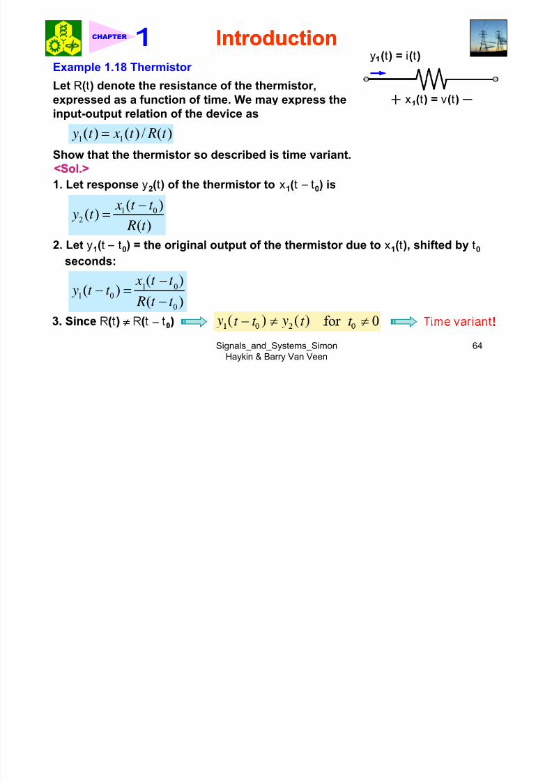
y ( ) ( )Example 1.18 Thermistor
Let R(t) denote the resistance of the thermistor,
expressed as a function of time. We may express the x1(t) = v(t)
input-output relation of the device as
1 1( ) ( ) / ( ) y t x t R t =
Show that the thermistor so described is time variant.
<Sol.><Sol.>
1. Let response y2(t) of the thermistor to x1(t t0) is
1 02
( )( ) ( )
x t t y t R t
−=
2. Let y1(t t0) = the original output of the thermistor due to x1(t), shifted by t0
seconds:
1 01 0
0
( )( )
y t t R t t
−− =−
≠ for 0t t t t − ≠ ≠
Signals_and_Systems_SimonHaykin & Barry Van Veen 64
≠
IntroductionIntroductionCHAPTER

8/13/2019 Ch01 Introduction Compatibility Mode
http://slidepdf.com/reader/full/ch01-introduction-compatibility-mode 65/98
★ .. .. near ynear y
A system is said to be linear in terms of the system input (excitation) x(t) andthe system output (response) y(t) if it satisfies the following two properties of
1. Superposition:
1( ) ( ) x t x t = 1( ) ( ) y t y t = 1 2( ) ( ) ( ) x t x t x t = +2( ) ( ) x t x t = 2( ) ( ) y t y t = 1 2( ) ( ) ( ) y t y t y t = +
2. Homogeneity: a = constant
( ) x t ( ) y t ( )ax t ( )ay t factor
♣ Linearity of continuous-time system
-. .
2. Input: N
x t a x t =
x1(t), x2(t), …, xN(t) ≡ input signal; a1, a2, …, aN ≡
Corresponding weighted factor
1i=
3. Output:( ) { ( )} { ( )}
N
i i y t H x t H a x t = = ∑ (1.87)
Signals_and_Systems_SimonHaykin & Barry Van Veen 65
1i=
IntroductionIntroductionCHAPTER
N

8/13/2019 Ch01 Introduction Compatibility Mode
http://slidepdf.com/reader/full/ch01-introduction-compatibility-mode 66/98
1( ) ( )
N
i ii
y t a y t == ∑ (1.88)
Superposition and
homogeneity
where
( ) { ( )}, 1, 2, ..., .i i y t H x t i N = = (1.89)
4. Commutation and Linearity:
1
( ) { ( )}i i
i
N
y t H a x t =
= ∑
1
{ ( )}i i
i N
a H x t
=
=
=
(1.90) Fig.Fig. 11..5656
1i i
i=
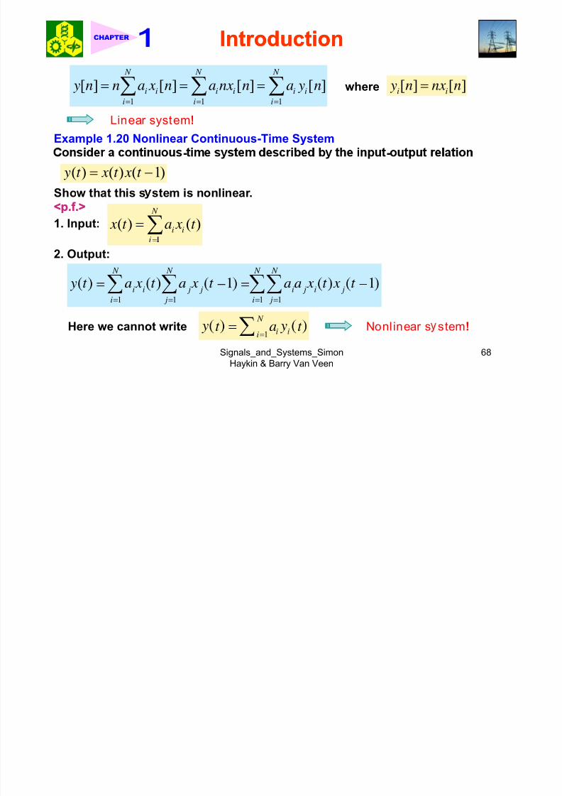
♣ Linearity of discrete-time system Same results, see ExampleExample 11..1919.
-.Consider a discrete-time system described by the input-output relation
[ ] [ ] y n nx n=
Signals_and_Systems_Simon
Haykin & Barry Van Veen
66
Show that this system is linear.
IntroductionIntroductionCHAPTER
8/13/2019 Ch01 Introduction Compatibility Mode
http://slidepdf.com/reader/full/ch01-introduction-compatibility-mode 67/98
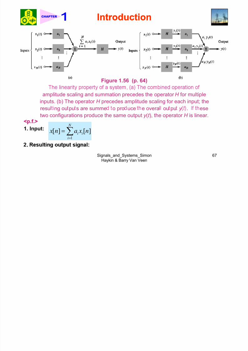
∑
Figure 1.56 (p. 64)
.
amplitude scaling and summation precedes the operator H for multipleinputs. (b) The operator H precedes amplitude scaling for each input; the
resu ng ou pu s are summe o pro uce e overa ou pu y . ese
two configurations produce the same output y (t ), the operator H is linear.<p.f.><p.f.>
N
1. Input:
1
[ ] [ ]i i
i
x n a x n=
= ∑
Signals_and_Systems_Simon
Haykin & Barry Van Veen
67
.
8/13/2019 Ch01 Introduction Compatibility Mode
http://slidepdf.com/reader/full/ch01-introduction-compatibility-mode 68/98
IntroductionIntroductionCHAPTER
Example 1 21 Impulse Response of RC Circuit

8/13/2019 Ch01 Introduction Compatibility Mode
http://slidepdf.com/reader/full/ch01-introduction-compatibility-mode 69/98
Example 1.21 Impulse Response of RC Circuit
For the RC circuit shown in Fig.Fig. 11..5757,determine the impulse response y(t).
FigureFigure 11..5757 (p.(p. 6666))
RC circuit for Example 1.20, in
<Sol.><Sol.>
1. Recall: Unit step response
/t RC −which we are given the capacitor
voltage y (t ) in response to the
step input x (t ) = y (t ) and the
,− .
2. Rectangular pulse input: Fig.Fig. 11..5858.
x t = x t
1/Δ
requirement is to find y (t ) in
response to the unit-impulseinput x (t ) = δ (t ).
11( ) ( ) x t u t Δ= +
Figure 1.58 (p. 66)
Rectangular pulse of unit2
1( ) ( )
2 x t u t
Δ= −
Δarea, w c , n e m ,approaches a unit impulse
as ∆→0.
3. Response to the step
functions x1(t) and x2(t):
Signals_and_Systems_Simon
Haykin & Barry Van Veen
69
−
IntroductionIntroductionCHAPTER
Δ ⎞⎛

8/13/2019 Ch01 Introduction Compatibility Mode
http://slidepdf.com/reader/full/ch01-introduction-compatibility-mode 70/98
/( )2
1 11 1 , ( ) ( )2
t RC
y e u t x t x t
Δ ⎞⎛ − +⎜ ⎟⎝ ⎠⎡ ⎤ Δ ⎞⎛ = − + =⎢ ⎥ ⎜ ⎟Δ ⎝ ⎠⎢ ⎥
/( )2
2 2
11 , ( ) ( )
t RC
y e u t x t x t
Δ ⎞⎛ − −⎜ ⎟⎝ ⎠
⎡ ⎤ Δ ⎞⎛ = − − =⎢ ⎥ ⎜ ⎟
Next, recognizing that
1 2 x x xΔ = −
( ) ( )( / 2) /( ) ( / 2) /( )1 1( ) (1 ) ( / 2) (1 ) ( / 2)
t RC t RC y t e u t e u t
− +Δ − −ΔΔ = − + Δ − − − Δ
( ) ( )( / 2) /( ) ( / 2) /( )1 1( ( / 2) ( / 2)) ( ( / 2) ) ( / 2))t RC t RC u t u t e u t e u t
− +Δ − −Δ= + Δ − − Δ − + Δ − − ΔΔ Δ
(1.92)i) δ(t) = the limiting form of the pulse x (t):
( ) lim ( )t x t δ =
Signals_and_Systems_Simon
Haykin & Barry Van Veen
70
0Δ→
IntroductionIntroductionCHAPTER
ii) The derivative of a continuous function of time say z(t):

8/13/2019 Ch01 Introduction Compatibility Mode
http://slidepdf.com/reader/full/ch01-introduction-compatibility-mode 71/98
ii) The derivative of a continuous function of time, say, z(t):
1lim
d z t z t z t
Δ Δ= + − −
0 2 2dt Δ→ Δ
0
( ) lim ( ) y t y t Δ
Δ→
=
/( ) ( ) ( ( ))t RC d t e u t
dt δ −= −
./( ) /( )
( ) ( ) ( ) ( )
t RC t RC d d
t e u t u t edt dt δ
− −
= − −/( ) /( ) ( ) ( ) ( ), ( ) ( )t RC t RC
t e t e u t x t t RC
δ δ δ − −= − + =
/( )1( ) ( ), ( ) ( )t RC y t e u t x t t
RC δ −= = (1.93)
Signals_and_Systems_Simon
Haykin & Barry Van Veen
71
IntroductionIntroductionCHAPTER
11 99 N iN i

8/13/2019 Ch01 Introduction Compatibility Mode
http://slidepdf.com/reader/full/ch01-introduction-compatibility-mode 72/98
11..99 NoiseNoiseNoise ⇒ Unwanted signals1. External sources of noise: atmospheric noise, galactic noise, and human-
made noise.2. Internal sources of noise: spontaneous fluctuations of the current or voltage
signal in electrical circuit. (electrical noise)
Fig.Fig. 11..6060..
★ 11..99..11 Thermal NoiseThermal Noise
Thermal noise arises from the random motion of electrons in a conductor.
Two characteristics of thermal noise:
1. Time-averaged value: 2T = total observation interval of noise
lim ( )2 T T
v v t dt T −→∞
= ∫ (1.94) As T → ∞, 0v → Refer to Fig.Refer to Fig. 11..6060..
2. Time-average-squared value: k = Boltzmann’s constant =
2 21lim ( )
2
T
T T v v t dt
T −→∞= ∫ (1.95)
→ 2 2
1.38 × 10 23 J/K
Tabs = absolute temperature
Signals_and_Systems_Simon
Haykin & Barry Van Veen
72
→ ∞, vo sabs
v = .
IntroductionIntroductionCHAPTER

8/13/2019 Ch01 Introduction Compatibility Mode
http://slidepdf.com/reader/full/ch01-introduction-compatibility-mode 73/98
Figure 1.60
(p. 68)
Sample waveform
of electrical noise
generated by a
thermionic diode
with a heated
cathode. Note
a e me-
averaged value ofthe noise voltage
approximately
zero.
Signals_and_Systems_Simon
Haykin & Barry Van Veen
73
IntroductionIntroductionCHAPTER
Thevenin’s equvalent circuit: Fig.Fig. 11..6161(a),(a), Norton’s equivalent circuit:

8/13/2019 Ch01 Introduction Compatibility Mode
http://slidepdf.com/reader/full/ch01-introduction-compatibility-mode 74/98
♣ Thevenin s equvalent circuit: Fig.Fig. 11..6161(a),(a), Norton s equivalent circuit:
Fig.Fig. 11..6161(b).(b).Noise voltage generator:
2( )v t v=Noise current generator:
2 2
2
lim ( )2
4 amps
T T
abs
i dt T R
kT G f
−→∞=
= Δ(1.97)
Figure 1.61 (p. 70)
where G = 1/R = conductance [S].
♣ Maximum power transfertheorem: the maximum
(a) Thévenin equivalent circuit of a noisy resistor.
(b) Norton equivalent circuit of the same resistor.possible power is transferred
from a source of internal
resistance Rl when R = Rl.
Under matched condition, the available power is
Signals_and_Systems_Simon
Haykin & Barry Van Veen
74
abs
IntroductionIntroductionCHAPTER
Two operating factor that affect available noise power:
8/13/2019 Ch01 Introduction Compatibility Mode
http://slidepdf.com/reader/full/ch01-introduction-compatibility-mode 75/98
♣ Two operating factor that affect available noise power:
1. The temperature at which the resistor is maintained.
2. The width of the fre uenc band over which the noise volta e across the
resistor is measured.
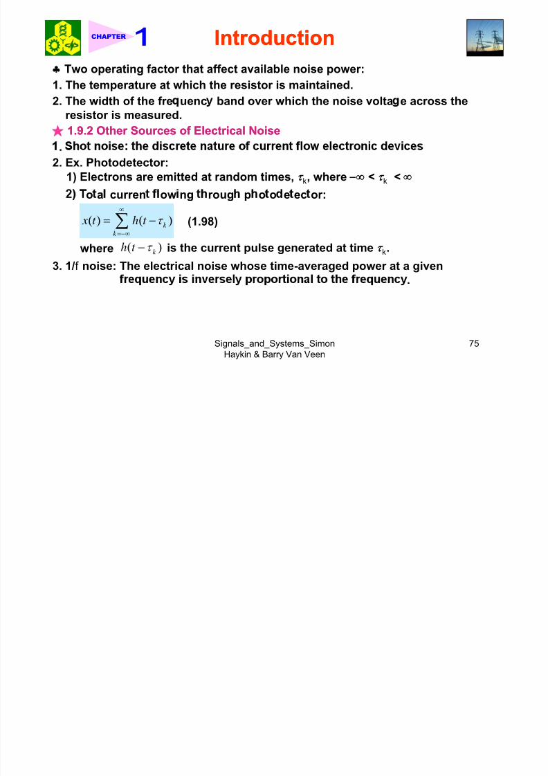
★ 11..99..22 Other Sources of Electrical NoiseOther Sources of Electrical Noise
.2. Ex. Photodetector:
1) Electrons are emitted at random times, τk, where ∞ < τk < ∞
o a curren ow ng roug p o o e ec or:
( ) ( )k
k
x t h t τ ∞
=−∞= −∑ (1.98)
( )k h t τ −where is the current pulse generated at time τk.
3. 1/f noise: The electrical noise whose time-averaged power at a given
.
Signals_and_Systems_Simon
Haykin & Barry Van Veen
75
IntroductionIntroductionCHAPTER
11..1010 Theme ExampleTheme Example

8/13/2019 Ch01 Introduction Compatibility Mode
http://slidepdf.com/reader/full/ch01-introduction-compatibility-mode 76/98
pp
★ 11..1010..11 Differentiation and Integration:Differentiation and Integration: RCRC CircuitsCircuits
1. Differentiator ⇒ Sharpening of a pulse
differentiator ( ) ( )
d y t x t
dt = (1.99)
mp e c rcu : g.g. .. .
2) Input-output relation:
1d d v t v t v t + = 1.100
Figure 1.62 (p. 71)
Simple RC circuit with small time
constant, used as an approximator
dt RC dt
If RC (time constant) is small enough
such that (1.100) is dominated by the
to a differentiator.second term v2(t)/RC, then
2 1
1( ) ( )
d v t v t ≈ 2 1( ) ( ) for small
d v t RC v t RC ≈ (1.101)
Signals_and_Systems_Simon
Haykin & Barry Van Veen
76
IntroductionIntroductionCHAPTER
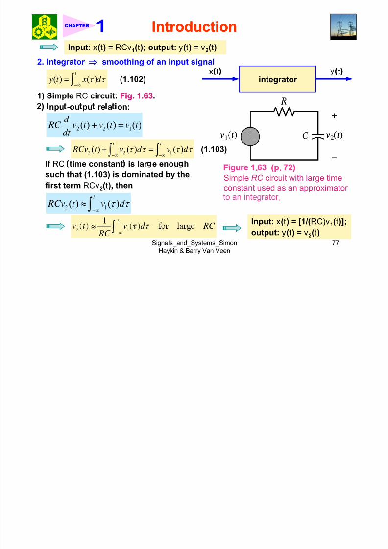
Input: x(t) = RCv1(t); output: y(t) = v2(t)
8/13/2019 Ch01 Introduction Compatibility Mode
http://slidepdf.com/reader/full/ch01-introduction-compatibility-mode 77/98
p ( ) 1( ) p y( ) 2( )
2. Integrator ⇒ smoothing of an input signal
x t t
1) Simple RC circuit: Fig.Fig. 11..6363.
integrator ( ) ( ) y t x d τ τ −∞
= (1.102)
npu -ou pu re a on:
2 2 1( ) ( ) ( )d
RC v t v t v t dt
+ =
2 2 1( ) ( ) ( )
t t
RCv t v d v d τ τ τ τ −∞ −∞+ =∫ ∫ (1.103)If RC time constant is lar e enou h
such that (1.103) is dominated by the
first term RCv2(t), then
. .
Simple RC circuit with large time
constant used as an approximator
2 1( ) ( ) RCv t v d τ τ −∞≈
1 t
≈
.
Input: x(t) = [1/(RC)v1(t)];
Signals_and_Systems_Simon
Haykin & Barry Van Veen
77
RC −∞ output: y(t) = v2(t)
IntroductionIntroductionCHAPTER
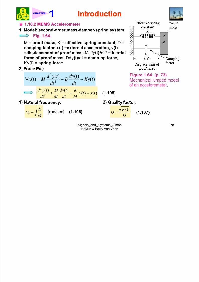
★ 11..1010..22 MEMS Accelerometer MEMS Accelerometer
8/13/2019 Ch01 Introduction Compatibility Mode
http://slidepdf.com/reader/full/ch01-introduction-compatibility-mode 78/98
1. Model: second-order mass-damper-spring system
Fig.Fig. 11..6464..
M = proof mass, K = effective spring constant, D =
damping factor, x(t) =external acceleration, y(t)
=dis lacement of roof mass Md2
t /dt2
= inertial force of proof mass, Ddy(t)/dt = damping force,
Ky(t) = spring force.
Figure 1.64 (p. 73)
Mechanical lumped model
. .2
2( ) ( )( ) ( )d y t dy t x t M D Ky t dt dt = + +
.2
2
( ) ( )( ) ( )
d y t D dy t K y t x t
dt M dt M + + = (1.105)
a ura requency:
n
K
M ω = (1.106)[rad/sec]
ua y ac or:KM
Q D
= (1.107)
Signals_and_Systems_Simon
Haykin & Barry Van Veen
78
IntroductionIntroductionCHAPTER
2
(1.105)2
2( ) ( )n
n
y y y t x t
ω ω + + = (1.108)

8/13/2019 Ch01 Introduction Compatibility Mode
http://slidepdf.com/reader/full/ch01-introduction-compatibility-mode 79/98
(1.105) 2( ) ( )n y
dt Q dt
(1.108)
★ 11..1010..33 Radar Range MeasurementRadar Range Measurement
1. A periodic sequence of radio frequency (RF) pulse: Fig.Fig. 11..6565.
T0 = duration [μsec], 1/T = repeated frequency, f c = RF frequency [MHz~GHz]
Figure 1.65 (p. 74)
Periodic train of rectangular FR pulses used for measuring molar ranges.
♣
Signals_and_Systems_Simon
Haykin & Barry Van Veen
79
♣ .

8/13/2019 Ch01 Introduction Compatibility Mode
http://slidepdf.com/reader/full/ch01-introduction-compatibility-mode 80/98
IntroductionIntroductionCHAPTER

8/13/2019 Ch01 Introduction Compatibility Mode
http://slidepdf.com/reader/full/ch01-introduction-compatibility-mode 81/98
Figure 1.66a(p. 75)
(a) Fluctuations in
the closing stock
price of Intel over
a three-year
period.
Signals_and_Systems_Simon
Haykin & Barry Van Veen
81
IntroductionIntroductionCHAPTER
8/13/2019 Ch01 Introduction Compatibility Mode
http://slidepdf.com/reader/full/ch01-introduction-compatibility-mode 82/98
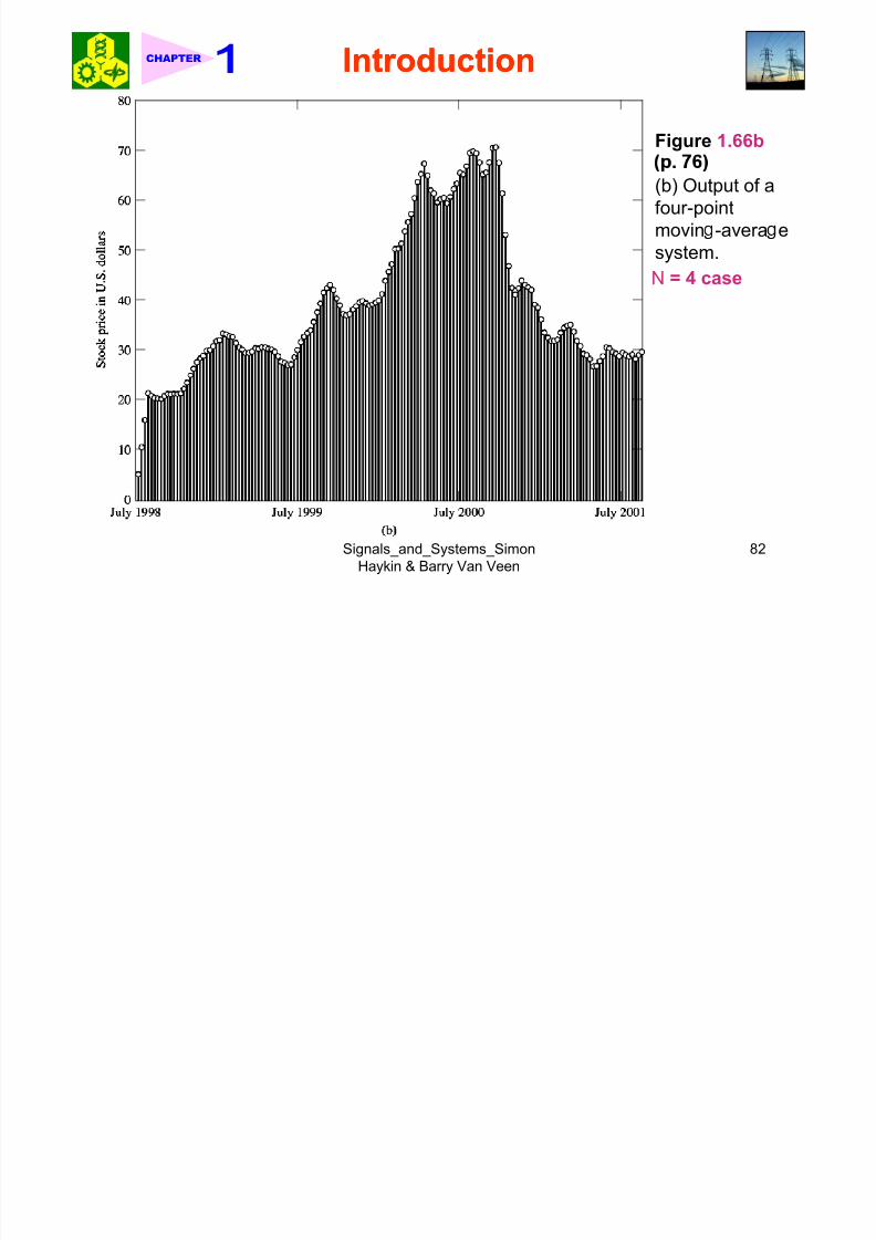
Figure 1.66b
(b) Output of a
four-point
movin -avera esystem.
N = 4 case
Signals_and_Systems_Simon
Haykin & Barry Van Veen
82
IntroductionIntroductionCHAPTER

8/13/2019 Ch01 Introduction Compatibility Mode
http://slidepdf.com/reader/full/ch01-introduction-compatibility-mode 83/98
Figure 1.66c(p. 76)
(c) Output of an
eight-point
moving-average
sys em.
N = 8 case
Signals_and_Systems_Simon
Haykin & Barry Van Veen
83
IntroductionIntroductionCHAPTER
2. For a general moving-average system, unequal weighting is applied to past

8/13/2019 Ch01 Introduction Compatibility Mode
http://slidepdf.com/reader/full/ch01-introduction-compatibility-mode 84/98
values of the input:1 N =
0k
k =
= − .
★ 11..1010..55 Multipath Communication ChannelsMultipath Communication Channels
. anne no se egra es e per ormance o a commun ca on sys em.
2. Another source of degradation of channel: dispersive nature, i.e., the channel
has memory.
3. For wireless system, the dispersive characteristics result from multipath
propagation.Fi .Fi . 11..6767..
♣ For a digital communication, multipath propagation manifests itself in the
form of intersymbol interference (ISI).
⇒. - ⇒ .. .. .
0
( ) ( ) p
i diff
i
y t x t iT ω =
= −∑ (1.112) Tdiff = smallest time difference
Signals_and_Systems_Simon
Haykin & Barry Van Veen
84
IntroductionIntroductionCHAPTER

8/13/2019 Ch01 Introduction Compatibility Mode
http://slidepdf.com/reader/full/ch01-introduction-compatibility-mode 85/98
Figure 1.67 (p. 77)
Signals_and_Systems_Simon
Haykin & Barry Van Veen
85
.
IntroductionIntroductionCHAPTER
8/13/2019 Ch01 Introduction Compatibility Mode
http://slidepdf.com/reader/full/ch01-introduction-compatibility-mode 86/98
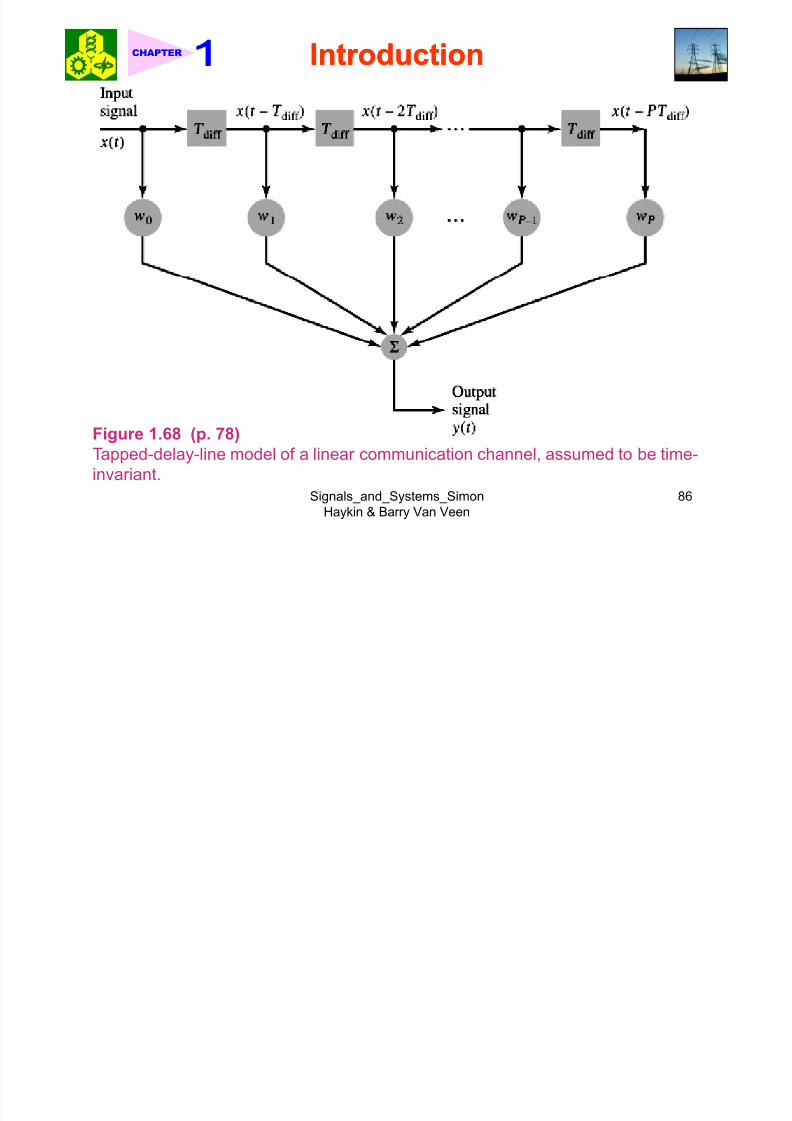
Figure 1.68 (p. 78)
Tapped-delay-line model of a linear communication channel, assumed to be time-
Signals_and_Systems_Simon
Haykin & Barry Van Veen
86
invariant.
IntroductionIntroductionCHAPTER
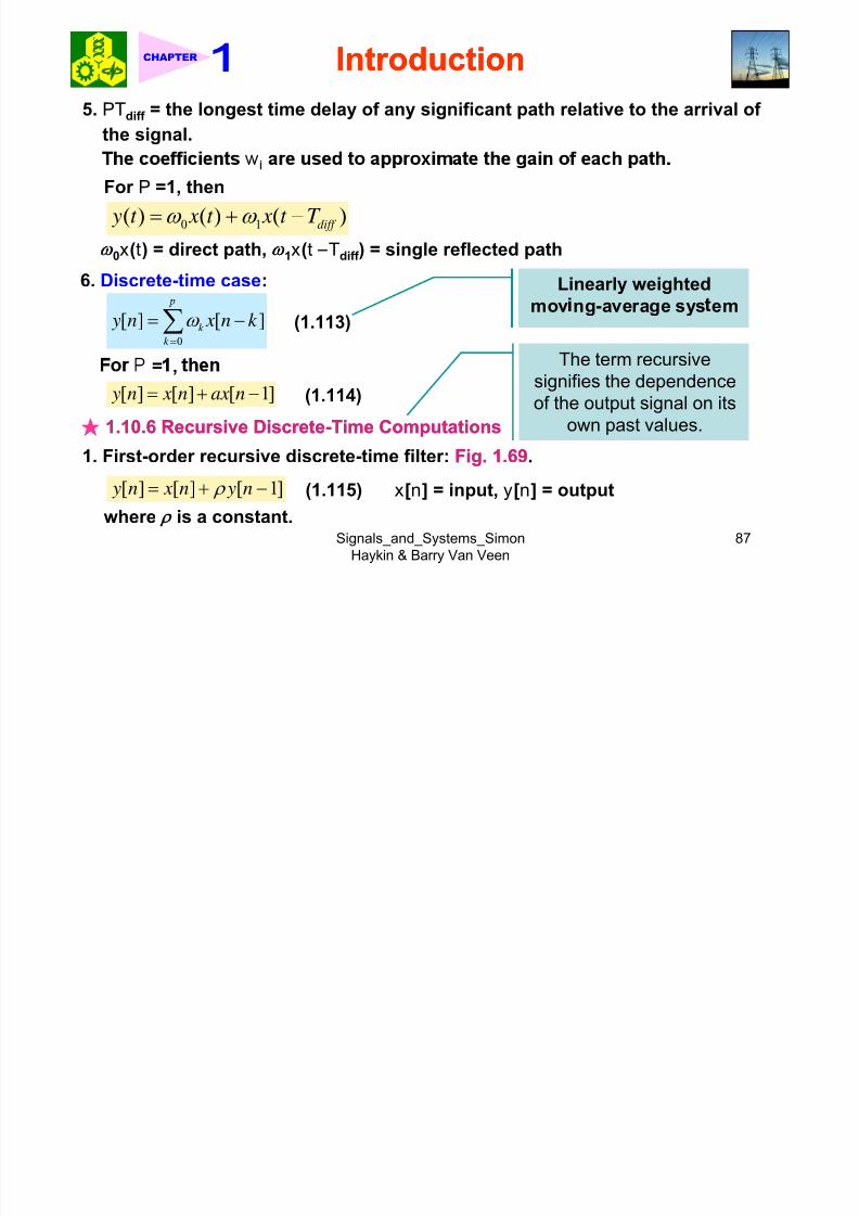
5. PTdiff = the longest time delay of any significant path relative to the arrival of
th i l
8/13/2019 Ch01 Introduction Compatibility Mode
http://slidepdf.com/reader/full/ch01-introduction-compatibility-mode 87/98
the signal.
For P =1, then
0 1( ) ( ) ( )diff
y t x t x t T ω ω = + −
ω0x(t) = direct path, ω1x(t Tdiff ) = single reflected path
6. Discrete-time case: Linearly weighted
0
[ ] [ ]k
k
y n x n k ω
=
= −∑ (1.113)
=
mov ng-average sys em
The term recursive,
[ ] [ ] [ 1] y n x n ax n= + − (1.114)
★ 11..1010..66 Recursive DiscreteRecursive Discrete--Time ComputationsTime Computations
signifies the dependence
of the output signal on its
own past values.
1. First-order recursive discrete-time filter: Fig.Fig. 11..6969.
x[n] = input, y[n] = output[ ] [ ] [ 1] y n x n y n ρ = + − (1.115)
Signals_and_Systems_Simon
Haykin & Barry Van Veen
87
where ρ is a constant.
IntroductionIntroductionCHAPTER
Figure 1.69 (p. 79)
Bl k di f fi t d

8/13/2019 Ch01 Introduction Compatibility Mode
http://slidepdf.com/reader/full/ch01-introduction-compatibility-mode 88/98
Block diagram of first-orderrecursive discrete-time filter. The
opera or s s e ou pu s gna
y [n] by one sampling interval,
producing y [n – 1]. The feedback
ρ stability of the filter.
♣ Fig. 1.69: linear discrete-time feedback system.
2. Solution of Eq.(1.115):
(1.116)[ ] [ ]k y n x n k ρ ∞
= −∑ r ≡ ρ
1
[ ] [ ] [ ]k
k
y n x n x n k ρ ∞
=
= + −∑
=
(1.117)
Setting k 1 = l , Eq.(1.117) becomes
1[ ] [ ] [ 1 ] [ ] [ 1 ]l l y n x n n l x n n l ρ ρ ρ
∞ ∞+= + − − = + − −∑ ∑ (1.118)
Signals_and_Systems_Simon
Haykin & Barry Van Veen
88
0 0l l= =
IntroductionIntroductionCHAPTER
[ ] [ ] [ 1] y n x n y n ρ = + −

8/13/2019 Ch01 Introduction Compatibility Mode
http://slidepdf.com/reader/full/ch01-introduction-compatibility-mode 89/98
3. Three special cases (depending on ρ):Accumulator
ρ = :
0
[ ] [ ]k
y n x n k ∞
=
= −∑(1.116) (1.119)
2) 1: ρ < Leaky accumulator
3) 1: ρ > Amplified accumulator
Stable in BIBO senseStable in BIBO sense
Unsatble inUnsatble in11..1111 Exploring Concepts with MATLABExploring Concepts with MATLAB
♣ MATLAB Signal Processing Toolbox1. Time vector: Sam lin interval T of 1 ms on the interval from 0 to 1 s
BIBO senseBIBO sense
t = 0:.001:1;
2. Vector n: n = 0:1000
★ 11..1111..11 Periodic SignalsPeriodic Signals
1. Square wave: A =amplitude, w0 = fundamental frequency, rho = duty cycle
Signals_and_Systems_Simon
Haykin & Barry Van Veen
89
square w , r o ;
IntroductionIntroductionCHAPTER
Ex. Obtain the square wave shown in Fig.Fig. 11..1414 (a)(a) by using MATLAB.
<Sol ><Sol > >> A = 1;

8/13/2019 Ch01 Introduction Compatibility Mode
http://slidepdf.com/reader/full/ch01-introduction-compatibility-mode 90/98
<Sol.><Sol.> >> A = 1;
>> w0 =10* i
>> rho = 0.5;
>> t = 0:.001:1;
>> s = A*s uare w0*t, rho ;
>> plot (t, sq)
>> axis([0 1 -1.1 1.1])
. , ,
A*sawtooth(w0*t, w);
Ex. Obtain the triangular wave shown in Fig.Fig. 11..1515 by using MATLAB.
>> A = 1;
>> w0 =10*pi;
=
<Sol.><Sol.>
.
>> t = 0:0.001:1;
>> tri = A*sawtooth(w0*t, w);
>>
Signals_and_Systems_Simon
Haykin & Barry Van Veen
90
,
IntroductionIntroductionCHAPTER
3. Discrete-time signal: stem(n, x);
x = vector n = discrete time vector

8/13/2019 Ch01 Introduction Compatibility Mode
http://slidepdf.com/reader/full/ch01-introduction-compatibility-mode 91/98
x = vector, n = discrete time vector Ex. Obtain the discrete-time s uare wave shown in Fi .Fi . 11..1616 b usin MATLAB.
>> A = 1;
>> omega =pi/4;
<Sol.><Sol.>
>> n = -10:10;>> x = A*square(omega*n);
>> stem(n, x)
4. Decaying exponential: B*exp(-a*t); Growing exponential: B*exp(a*t);
Ex. Obtain the decaying exponential signal shown in Fig.Fig. 11..2828 (a)(a) by using
.
>> B = 5;
>> a = 6;
<Sol.><Sol.>
>> = :. : ;>> x = B*exp(-a*t); % decaying exponential
>> plot (t, x)
Signals_and_Systems_Simon
Haykin & Barry Van Veen
91
IntroductionIntroductionCHAPTER
Ex. Obtain the growing exponential signal shown in Fig.Fig. 11..2828 (b)(b) by using
MATLAB

8/13/2019 Ch01 Introduction Compatibility Mode
http://slidepdf.com/reader/full/ch01-introduction-compatibility-mode 92/98
MATLAB.>> B = 1;
<Sol.><Sol.>
>> a = 5;
>> t = 0:0.001:1;
>> x = B*exp(a*t); % growing exponential
>> plot (t, x)
Ex. Obtain the decaying exponential sequence shown in Fig.Fig. 11..3030 (a)(a) by using
.<Sol.><Sol.>
>> B = 1;
>> r = 0.85;
>> n = - : ;
>> x = B*r.^n; % decaying exponential sequence
>> stem (n, x)
★ 11..1111..33 Sinusoidal SignalsSinusoidal Signals
1. Cosine signal: 2. Sine signal:
A = amplitude, w0 =frequency, phi =
phase angle
Signals_and_Systems_Simon
Haykin & Barry Van Veen
92
cos w p ; s n w p ;
IntroductionIntroductionCHAPTER
Ex. Obtain the sinusoidal signal shown in Fig.Fig. 11..3131 (a)(a) by using MATLAB.
>> A = 4;<Sol ><Sol >

8/13/2019 Ch01 Introduction Compatibility Mode
http://slidepdf.com/reader/full/ch01-introduction-compatibility-mode 93/98
>> A = 4;
>> w0 =20* i
<Sol.><Sol.>
>> phi = pi/6;
>> t = 0:.001:1;
>> cosine = A*cos w0*t + hi ;
>> plot (t, cosine)
Ex. Obtain the discrete-time sinusoidal signal shown in Fig.Fig. 11..3333 by using
.
>> A = 1;
>> omega =2*pi/12; % angular frequency
<Sol.><Sol.>
.*.* ≡ element-by-element>> n = - : ;
>> y = A*cos(omega*n);
>> stem (n, y)
mu p ca on
★ 11..1111..44 Exponential Damped Sinusoidal SignalsExponential Damped Sinusoidal Signals1. Exponentially damped sinusoidal signal:
at −= * * * - *
Signals_and_Systems_Simon
Haykin & Barry Van Veen
93
0 .
IntroductionIntroductionCHAPTER
Ex. Obtain the waveform shown in Fig.Fig. 11..3535 by using MATLAB.
<Sol ><Sol > >> A = 60;

8/13/2019 Ch01 Introduction Compatibility Mode
http://slidepdf.com/reader/full/ch01-introduction-compatibility-mode 94/98
<Sol.><Sol.> >> A 60;>> w0 =20* i
>> phi = 0;
>> a = 6;
>> t = 0:.001:1;
>> expsin = A*sin(w0*t + phi).*exp(-a*t);
>> plot (t, expsin)
. .. ..
using MATLAB.
<Sol.><Sol.> >> A = 1;
>> omega =2*pi/12; % angular frequency
>> n = -10:10;
>> y = A*cos(omega*n);
>> r = . ;>> x = A*r.^n; % decaying exponential sequence
>> z = x.*y; % elementwise multiplication
Signals_and_Systems_Simon
Haykin & Barry Van Veen
94
s em n, z
IntroductionIntroductionCHAPTER

8/13/2019 Ch01 Introduction Compatibility Mode
http://slidepdf.com/reader/full/ch01-introduction-compatibility-mode 95/98
Figure 1.70 (p. 84)
Signals_and_Systems_Simon
Haykin & Barry Van Veen
95
.
IntroductionIntroductionCHAPTER
★ 11..1111..55 Step, Impulse, and Ramp FunctionsStep, Impulse, and Ramp Functions
MATLAB command:
Ex.Ex. Generate a rectangular pulse
centered at origin on the interval[ 1 1]

8/13/2019 Ch01 Introduction Compatibility Mode
http://slidepdf.com/reader/full/ch01-introduction-compatibility-mode 96/98
MATLAB command:1. M-by-N matrix of ones: ones (M, N)
centered at origin on the interval[-1, 1].
2. M-by-N matrix of zeros: zeros (M, N)
♣ Unit amplitude step function:
<Sol.><Sol.>
= -u = zeros , , ones , ;
♣ Discrete-time impulse:
=
>> u1 = [zeros(1, 250), ones(1, 751)];
>> u2 = [zeros(1, 751), ones(1, 250)];
> > u = u 1 – u 2 , , , ,
♣ Ramp sequence:
ramp = 0:.1:10
★ 11..1111..66 User User--Defined FunctionsDefined Functions
1. Two types M-files exist: scripts and functions.
cr p s, or scr p es au oma e ong sequences o comman s; unc ons, orfunction files, provide extensibility to MATLAB by allowing us to add new functions.
2. Procedure for establishing a function M-file:
Signals_and_Systems_Simon
Haykin & Barry Van Veen
96
IntroductionIntroductionCHAPTER
1) It begins with a statement defining the function name, its input arguments, and
its output arguments.2) It also includes additional statements that compute the values to be returned

8/13/2019 Ch01 Introduction Compatibility Mode
http://slidepdf.com/reader/full/ch01-introduction-compatibility-mode 97/98
p g2) It also includes additional statements that compute the values to be returned.
e npu s may e sca ars, vec ors, or ma r ces.
Ex. Obtain the rectangular pulse depicted in Fig.Fig. 11..3939 (a)(a) with the use of an
M-file.
-< o .>< o .>>> function g = rect(x)
>> g = zeros(size(x));
>> = <=
. element vector containing the row
and column dimensions of a matrix.
.
>> g(set1) = ones(size(set1));
.
indices of a vector or matrix that
satisfy a prescribed relation3. The new function rect.m can be used
Ex. find(abs(x)<= T) returns the indices
of the vector x, where the absolute
.
>> = -
Ex. To generate a rectangular pulse:
.
>> plot(t, rect(t));
Signals_and_Systems_Simon
Haykin & Barry Van Veen
97
IntroductionIntroductionCHAPTER

8/13/2019 Ch01 Introduction Compatibility Mode
http://slidepdf.com/reader/full/ch01-introduction-compatibility-mode 98/98
Signals_and_Systems_Simon
Haykin & Barry Van Veen
98

![Electrochemistry [Compatibility Mode]](https://static.fdocuments.in/doc/165x107/54e793294a7959397d8b495f/electrochemistry-compatibility-mode.jpg)
![12 [compatibility mode]](https://static.fdocuments.in/doc/165x107/54454664afaf9f14098b45ce/12-compatibility-mode.jpg)
![Reciprocatingcom [Compatibility Mode]](https://static.fdocuments.in/doc/165x107/55cf8fca550346703b9fe10b/reciprocatingcom-compatibility-mode.jpg)
![SmallFarm.ppt [Compatibility Mode]](https://static.fdocuments.in/doc/165x107/5486beafb47959f10c8b52d4/smallfarmppt-compatibility-mode.jpg)
![salkind ppt ch01 - Troy Universityspectrum.troy.edu/drsmall/Class Stuff/Cp6691/Salkind/Mid-Term PP'… · Microsoft PowerPoint - salkind_ppt_ch01 [Compatibility Mode] Author: Lamon](https://static.fdocuments.in/doc/165x107/60099061a2786e0bcd750be9/salkind-ppt-ch01-troy-stuffcp6691salkindmid-term-pp-microsoft-powerpoint.jpg)
![Mitosis [compatibility mode]](https://static.fdocuments.in/doc/165x107/558d4aedd8b42aa9108b46e7/mitosis-compatibility-mode.jpg)
![iterative), in which the basic sciences, mathematics,erives/382_10/Ch01.pdf · Microsoft PowerPoint - Ch01.ppt [Compatibility Mode] Author: Hector Created Date: 1/21/2010 2:59:41](https://static.fdocuments.in/doc/165x107/5f9763eda7a3d56264274f67/iterative-in-which-the-basic-sciences-mathematics-erives38210ch01pdf-microsoft.jpg)
![Solution [Compatibility Mode]](https://static.fdocuments.in/doc/165x107/55cf8e3e550346703b900ca9/solution-compatibility-mode.jpg)
![Ch01 [Compatibility Mode]](https://static.fdocuments.in/doc/165x107/577d25651a28ab4e1e9eb28f/ch01-compatibility-mode.jpg)
![Connection_Design [Compatibility Mode]](https://static.fdocuments.in/doc/165x107/55cf8f33550346703b99ea87/connectiondesign-compatibility-mode.jpg)
![sISTEMOPERASI [Compatibility Mode]](https://static.fdocuments.in/doc/165x107/5571ff3249795991699ccfd9/sistemoperasi-compatibility-mode.jpg)
![09 [compatibility mode]](https://static.fdocuments.in/doc/165x107/55a5ad7d1a28aba5238b46e2/09-compatibility-mode.jpg)
![Meas.association [compatibility mode]](https://static.fdocuments.in/doc/165x107/55a7165c1a28ab1f358b48cf/measassociation-compatibility-mode.jpg)
![SIMPUSTRONIK [Compatibility Mode]](https://static.fdocuments.in/doc/165x107/547f5b55b47959a2508b4ea1/simpustronik-compatibility-mode.jpg)
![DTH [Compatibility Mode]](https://static.fdocuments.in/doc/165x107/544f4cd3af7959e51e8b52d5/dth-compatibility-mode.jpg)
![LOPA [Compatibility Mode]](https://static.fdocuments.in/doc/165x107/55cf9a0e550346d033a04659/lopa-compatibility-mode.jpg)
![CH01 [Compatibility Mode].pdf](https://static.fdocuments.in/doc/165x107/577cd68c1a28ab9e789cab39/ch01-compatibility-modepdf.jpg)
![Getting Started: Principals of Financepthistle.faculty.unlv.edu/FIN301_Spring2019/Slides_S2019/Ch01Full.pdfMicrosoft PowerPoint - Ch01.S19 (1) [Compatibility Mode] Author: pthistle](https://static.fdocuments.in/doc/165x107/5f43a07af5dfdf13347405ee/getting-started-principals-of-microsoft-powerpoint-ch01s19-1-compatibility.jpg)