Ch Mechanism Toolkit - softintegration.com
499
Ch Mechanism Toolkit Version 3.0 User’s Guide
Transcript of Ch Mechanism Toolkit - softintegration.com

Ch Mechanism ToolkitVersion 3.0
User’s Guide

How to Contact SoftIntegration
Mail SoftIntegration, Inc.
216 F Street, #68
Davis, CA 95616
Phone + 1 530 297 7398
Fax + 1 530 297 7392
Web http://www.softintegration.com
Email [email protected]
Copyright c©2004-2015 by SoftIntegration, Inc. All rights reserved.
Revision 3.0.0, December, 2015
No part of this publication may be reproduced, stored in a retrieval system, or transmitted, in any form
or by any means, electronic, mechanical, photocopying, recording, or otherwise, without the prior written
permission of the copyright holder.
SoftIntegration, Inc. is the holder of the copyright to the Ch Mechanism Toolkit described in this document.
SoftIntegration, Inc. makes no representations, expressed or implied, with respect to this documenta-
tion, or the software it describes, including without limitations, any implied warranty merchantability
or fitness for a particular purpose, all of which are expressly disclaimed. Users should be aware that
included in the terms and conditions under which SoftIntegration is willing to license the Ch Mech-
anism Toolkit as a provision that SoftIntegration, and their distribution licensees, distributors and
dealers shall in no event be liable for any indirect, incidental or consequential damages in connection
with, or arising out of, the furnishing, performance, or use of the Ch Mechanism Toolkit, and that lia-
bility for direct damages shall be limited to the amount of purchase price paid for the Ch Mechanism
Toolkit.
Ch, SoftIntegration, One Language for All, and Quick Animation are either registered trademarks or trade-
marks of SoftIntegration, Inc. in the United States and/or other countries. Microsoft, MS-DOS, Windows,
Windows 95, Windows 98, Windows Me, Windows NT, Windows 2000, and Windows XP are trademarks
of Microsoft Corporation. Solaris and Sun are trademarks of Sun Microsystems, Inc. Unix is a trademark
of the Open Group. HP-UX is either a registered trademark or a trademark of Hewlett-Packard Co. Linux
is a trademark of Linus Torvalds. All other trademarks belong to their respective holders.
ii

Table of Contents
1 Getting Started with Ch Mechanism Toolkit 1
1.1 Introduction . . . . . . . . . . . . . . . . . . . . . . . . . . . . . . . . . . . . . . . . . . . 1
1.2 Features . . . . . . . . . . . . . . . . . . . . . . . . . . . . . . . . . . . . . . . . . . . . . 1
1.3 Getting Started . . . . . . . . . . . . . . . . . . . . . . . . . . . . . . . . . . . . . . . . . 2
1.4 Solving Complex Equations . . . . . . . . . . . . . . . . . . . . . . . . . . . . . . . . . . 5
1.4.1 Solving for Two Angles Using complexsolveRR() . . . . . . . . . . . . . . . . . . 6
1.4.2 Solving for One Displacement and One Angle Using complexsolvePR() . . . . . . . 6
1.4.3 Solving for Two Displacements Using complexsolvePP() . . . . . . . . . . . . . . . 7
1.4.4 Solving for One Displacement and One Angle Using complexsolveRP() . . . . . . . 8
1.4.5 Solving for Two Angles Using complexsolveRRz() . . . . . . . . . . . . . . . . . . 9
2 Fourbar Linkage 11
2.1 Position Analysis . . . . . . . . . . . . . . . . . . . . . . . . . . . . . . . . . . . . . . . . 11
2.2 Transmission Angle Analysis . . . . . . . . . . . . . . . . . . . . . . . . . . . . . . . . . . 19
2.3 Velocity Analysis . . . . . . . . . . . . . . . . . . . . . . . . . . . . . . . . . . . . . . . . 21
2.4 Acceleration Analysis . . . . . . . . . . . . . . . . . . . . . . . . . . . . . . . . . . . . . . 23
2.5 Dynamics . . . . . . . . . . . . . . . . . . . . . . . . . . . . . . . . . . . . . . . . . . . . 24
2.6 Kinematics and Dynamics with Constant Angular Velocity for Link 2 . . . . . . . . . . . . 28
2.7 Three-Position Synthesis . . . . . . . . . . . . . . . . . . . . . . . . . . . . . . . . . . . . 34
2.8 Animation . . . . . . . . . . . . . . . . . . . . . . . . . . . . . . . . . . . . . . . . . . . . 36
2.9 Web-Based Fourbar Linkage Analysis . . . . . . . . . . . . . . . . . . . . . . . . . . . . . 40
2.9.1 Position Analysis . . . . . . . . . . . . . . . . . . . . . . . . . . . . . . . . . . . . 40
2.9.2 Coupler Curve Plotting . . . . . . . . . . . . . . . . . . . . . . . . . . . . . . . . . 40
2.9.3 Animation . . . . . . . . . . . . . . . . . . . . . . . . . . . . . . . . . . . . . . . 40
3 Crank-Slider Mechanism 48
3.1 Position Analysis . . . . . . . . . . . . . . . . . . . . . . . . . . . . . . . . . . . . . . . . 49
3.2 Transmission Angles . . . . . . . . . . . . . . . . . . . . . . . . . . . . . . . . . . . . . . 53
3.3 Velocity Analysis . . . . . . . . . . . . . . . . . . . . . . . . . . . . . . . . . . . . . . . . 53
3.4 Acceleration Analysis . . . . . . . . . . . . . . . . . . . . . . . . . . . . . . . . . . . . . . 55
3.5 Position, Velocity and Acceleration of Coupler Point . . . . . . . . . . . . . . . . . . . . . 56
3.6 Dynamic Force Analysis . . . . . . . . . . . . . . . . . . . . . . . . . . . . . . . . . . . . 57
3.7 Animation . . . . . . . . . . . . . . . . . . . . . . . . . . . . . . . . . . . . . . . . . . . . 63
3.8 Web-Based Crank-Slider Linkage Analysis . . . . . . . . . . . . . . . . . . . . . . . . . . 66
iii

4 Geared Five-Bar Linkage 82
4.1 Position Analysis . . . . . . . . . . . . . . . . . . . . . . . . . . . . . . . . . . . . . . . . 82
4.2 Velocity Analysis . . . . . . . . . . . . . . . . . . . . . . . . . . . . . . . . . . . . . . . . 83
4.3 Acceleration Analysis . . . . . . . . . . . . . . . . . . . . . . . . . . . . . . . . . . . . . . 85
4.4 Coupler Point Analysis . . . . . . . . . . . . . . . . . . . . . . . . . . . . . . . . . . . . . 85
4.5 Animation . . . . . . . . . . . . . . . . . . . . . . . . . . . . . . . . . . . . . . . . . . . . 86
4.6 Web-Based Geared Fivebar Linkage Analysis . . . . . . . . . . . . . . . . . . . . . . . . . 86
5 Multi-Loop Six-Bar Linkages 95
5.1 Fourbar/Slider-Crank Linkage . . . . . . . . . . . . . . . . . . . . . . . . . . . . . . . . . 95
5.1.1 Position Analysis . . . . . . . . . . . . . . . . . . . . . . . . . . . . . . . . . . . . 95
5.1.2 Velocity Analysis . . . . . . . . . . . . . . . . . . . . . . . . . . . . . . . . . . . . 98
5.1.3 Acceleration Analysis . . . . . . . . . . . . . . . . . . . . . . . . . . . . . . . . . 99
5.1.4 Animation . . . . . . . . . . . . . . . . . . . . . . . . . . . . . . . . . . . . . . . 102
5.1.5 Web-Based Fourbar-Slider Linkage Analysis . . . . . . . . . . . . . . . . . . . . . 103
5.2 Watt Six-bar (I) Linkage . . . . . . . . . . . . . . . . . . . . . . . . . . . . . . . . . . . . 110
5.2.1 Position Analysis . . . . . . . . . . . . . . . . . . . . . . . . . . . . . . . . . . . . 111
5.2.2 Velocity Analysis . . . . . . . . . . . . . . . . . . . . . . . . . . . . . . . . . . . . 111
5.2.3 Acceleration Analysis . . . . . . . . . . . . . . . . . . . . . . . . . . . . . . . . . 112
5.2.4 Coupler Position, Velocity, and Acceleration . . . . . . . . . . . . . . . . . . . . . 114
5.2.5 Animation . . . . . . . . . . . . . . . . . . . . . . . . . . . . . . . . . . . . . . . 116
5.2.6 Web-Based Analysis . . . . . . . . . . . . . . . . . . . . . . . . . . . . . . . . . . 119
5.3 Watt Six-bar (II) Linkage . . . . . . . . . . . . . . . . . . . . . . . . . . . . . . . . . . . . 127
5.3.1 Position Analysis . . . . . . . . . . . . . . . . . . . . . . . . . . . . . . . . . . . . 127
5.3.2 Velocity Analysis . . . . . . . . . . . . . . . . . . . . . . . . . . . . . . . . . . . . 128
5.3.3 Acceleration Analysis . . . . . . . . . . . . . . . . . . . . . . . . . . . . . . . . . 129
5.3.4 Coupler Point Position, Velocity, and Acceleration . . . . . . . . . . . . . . . . . . 131
5.3.5 Input/Output Ranges . . . . . . . . . . . . . . . . . . . . . . . . . . . . . . . . . . 135
5.3.6 Animation . . . . . . . . . . . . . . . . . . . . . . . . . . . . . . . . . . . . . . . 136
5.3.7 Web-Based Analysis . . . . . . . . . . . . . . . . . . . . . . . . . . . . . . . . . . 137
5.4 Stephenson Six-bar (I) Linkage . . . . . . . . . . . . . . . . . . . . . . . . . . . . . . . . . 144
5.4.1 Position Analysis . . . . . . . . . . . . . . . . . . . . . . . . . . . . . . . . . . . . 144
5.4.2 Velocity Analysis . . . . . . . . . . . . . . . . . . . . . . . . . . . . . . . . . . . . 145
5.4.3 Acceleration Analysis . . . . . . . . . . . . . . . . . . . . . . . . . . . . . . . . . 146
5.4.4 Coupler Point Position, Velocity, and Acceleration . . . . . . . . . . . . . . . . . . 151
5.4.5 Animation . . . . . . . . . . . . . . . . . . . . . . . . . . . . . . . . . . . . . . . 151
5.4.6 Web-Based Analysis . . . . . . . . . . . . . . . . . . . . . . . . . . . . . . . . . . 153
5.5 Stephenson Six-bar (III) Linkage . . . . . . . . . . . . . . . . . . . . . . . . . . . . . . . . 154
5.5.1 Position Analysis . . . . . . . . . . . . . . . . . . . . . . . . . . . . . . . . . . . . 161
5.5.2 Velocity Analysis . . . . . . . . . . . . . . . . . . . . . . . . . . . . . . . . . . . . 161
5.5.3 Acceleration Analysis . . . . . . . . . . . . . . . . . . . . . . . . . . . . . . . . . 162
5.5.4 Coupler Point Position, Velocity, and Acceleration . . . . . . . . . . . . . . . . . . 165
5.5.5 Animation . . . . . . . . . . . . . . . . . . . . . . . . . . . . . . . . . . . . . . . 165
5.5.6 Web-Based Analysis . . . . . . . . . . . . . . . . . . . . . . . . . . . . . . . . . . 167
iv

6 Cam Design 176
6.1 Introduction to Cam Design . . . . . . . . . . . . . . . . . . . . . . . . . . . . . . . . . . . 176
6.2 Cam Design with Class CCam . . . . . . . . . . . . . . . . . . . . . . . . . . . . . . . . . 180
6.3 Web-Based Cam Design . . . . . . . . . . . . . . . . . . . . . . . . . . . . . . . . . . . . 194
7 Quick Animation 201
7.1 The User Interface for QuickAnimationTM . . . . . . . . . . . . . . . . . . . . . . . . . . 202
7.2 Input Data Format . . . . . . . . . . . . . . . . . . . . . . . . . . . . . . . . . . . . . . . . 202
7.2.1 General Drawing Primitives . . . . . . . . . . . . . . . . . . . . . . . . . . . . . . 202
7.2.2 Mechanical Drawing Primitives . . . . . . . . . . . . . . . . . . . . . . . . . . . . 205
7.3 Quick Animation Examples . . . . . . . . . . . . . . . . . . . . . . . . . . . . . . . . . . . 207
8 Implementations of Interactive Web Pages for Mechanism Design and Analysis 220
8.1 Introduction to CGI Programming . . . . . . . . . . . . . . . . . . . . . . . . . . . . . . . 220
8.1.1 Writing HTML Files . . . . . . . . . . . . . . . . . . . . . . . . . . . . . . . . . . 220
8.1.2 Writing CGI Script Files . . . . . . . . . . . . . . . . . . . . . . . . . . . . . . . . 223
8.2 Web-Based Animation Example . . . . . . . . . . . . . . . . . . . . . . . . . . . . . . . . 225
8.2.1 Configuration and Setup of Web Servers . . . . . . . . . . . . . . . . . . . . . . . . 226
9 References 236
A Header File linkage.h 237
linkage.h . . . . . . . . . . . . . . . . . . . . . . . . . . . . . . . . . . . . . . . . . . . . . . . . 237
B Class CFourbar 239
CFourbar . . . . . . . . . . . . . . . . . . . . . . . . . . . . . . . . . . . . . . . . . . . . . . . 239
angularAccel . . . . . . . . . . . . . . . . . . . . . . . . . . . . . . . . . . . . . . . . . . 241
angularAccels . . . . . . . . . . . . . . . . . . . . . . . . . . . . . . . . . . . . . . . . . . 243
angularPos . . . . . . . . . . . . . . . . . . . . . . . . . . . . . . . . . . . . . . . . . . . . 244
angularPoss . . . . . . . . . . . . . . . . . . . . . . . . . . . . . . . . . . . . . . . . . . . 245
angularVel . . . . . . . . . . . . . . . . . . . . . . . . . . . . . . . . . . . . . . . . . . . . 247
angularVels . . . . . . . . . . . . . . . . . . . . . . . . . . . . . . . . . . . . . . . . . . . 248
animation . . . . . . . . . . . . . . . . . . . . . . . . . . . . . . . . . . . . . . . . . . . . 250
couplerCurve . . . . . . . . . . . . . . . . . . . . . . . . . . . . . . . . . . . . . . . . . . 258
couplerPointAccel . . . . . . . . . . . . . . . . . . . . . . . . . . . . . . . . . . . . . . . . 261
couplerPointPos . . . . . . . . . . . . . . . . . . . . . . . . . . . . . . . . . . . . . . . . . 262
couplerPointVel . . . . . . . . . . . . . . . . . . . . . . . . . . . . . . . . . . . . . . . . . 263
displayPosition . . . . . . . . . . . . . . . . . . . . . . . . . . . . . . . . . . . . . . . . . 265
displayPositions . . . . . . . . . . . . . . . . . . . . . . . . . . . . . . . . . . . . . . . . . 267
forceTorque . . . . . . . . . . . . . . . . . . . . . . . . . . . . . . . . . . . . . . . . . . . 267
forceTorques . . . . . . . . . . . . . . . . . . . . . . . . . . . . . . . . . . . . . . . . . . 269
getAngle . . . . . . . . . . . . . . . . . . . . . . . . . . . . . . . . . . . . . . . . . . . . . 272
getJointLimits . . . . . . . . . . . . . . . . . . . . . . . . . . . . . . . . . . . . . . . . . . 272
grashof . . . . . . . . . . . . . . . . . . . . . . . . . . . . . . . . . . . . . . . . . . . . . 274
plotAngularAccels . . . . . . . . . . . . . . . . . . . . . . . . . . . . . . . . . . . . . . . 275
plotAngularPoss . . . . . . . . . . . . . . . . . . . . . . . . . . . . . . . . . . . . . . . . . 276
plotAngularVels . . . . . . . . . . . . . . . . . . . . . . . . . . . . . . . . . . . . . . . . . 278
plotCouplerCurve . . . . . . . . . . . . . . . . . . . . . . . . . . . . . . . . . . . . . . . . 279
v

plotForceTorques . . . . . . . . . . . . . . . . . . . . . . . . . . . . . . . . . . . . . . . . 280
plotTransAngles . . . . . . . . . . . . . . . . . . . . . . . . . . . . . . . . . . . . . . . . . 281
printJointLimits . . . . . . . . . . . . . . . . . . . . . . . . . . . . . . . . . . . . . . . . . 282
setAngularVel . . . . . . . . . . . . . . . . . . . . . . . . . . . . . . . . . . . . . . . . . . 283
setCouplerPoint . . . . . . . . . . . . . . . . . . . . . . . . . . . . . . . . . . . . . . . . . 284
setGravityCenter . . . . . . . . . . . . . . . . . . . . . . . . . . . . . . . . . . . . . . . . 285
setInertia . . . . . . . . . . . . . . . . . . . . . . . . . . . . . . . . . . . . . . . . . . . . 285
setLinks . . . . . . . . . . . . . . . . . . . . . . . . . . . . . . . . . . . . . . . . . . . . . 286
setMass . . . . . . . . . . . . . . . . . . . . . . . . . . . . . . . . . . . . . . . . . . . . . 286
setNumPoints . . . . . . . . . . . . . . . . . . . . . . . . . . . . . . . . . . . . . . . . . . 287
synthesis . . . . . . . . . . . . . . . . . . . . . . . . . . . . . . . . . . . . . . . . . . . . . 287
transAngle . . . . . . . . . . . . . . . . . . . . . . . . . . . . . . . . . . . . . . . . . . . . 289
transAngles . . . . . . . . . . . . . . . . . . . . . . . . . . . . . . . . . . . . . . . . . . . 290
uscUnit . . . . . . . . . . . . . . . . . . . . . . . . . . . . . . . . . . . . . . . . . . . . . 291
C Class CCrankSlider 293
CCrankSlider . . . . . . . . . . . . . . . . . . . . . . . . . . . . . . . . . . . . . . . . . . . . . 293
angularAccel . . . . . . . . . . . . . . . . . . . . . . . . . . . . . . . . . . . . . . . . . . 294
angularPos . . . . . . . . . . . . . . . . . . . . . . . . . . . . . . . . . . . . . . . . . . . . 296
angularVel . . . . . . . . . . . . . . . . . . . . . . . . . . . . . . . . . . . . . . . . . . . . 297
animation . . . . . . . . . . . . . . . . . . . . . . . . . . . . . . . . . . . . . . . . . . . . 298
couplerCurve . . . . . . . . . . . . . . . . . . . . . . . . . . . . . . . . . . . . . . . . . . 299
couplerPointAccel . . . . . . . . . . . . . . . . . . . . . . . . . . . . . . . . . . . . . . . . 301
couplerPointPos . . . . . . . . . . . . . . . . . . . . . . . . . . . . . . . . . . . . . . . . . 302
couplerPointVel . . . . . . . . . . . . . . . . . . . . . . . . . . . . . . . . . . . . . . . . . 303
displayPosition . . . . . . . . . . . . . . . . . . . . . . . . . . . . . . . . . . . . . . . . . 304
forceTorque . . . . . . . . . . . . . . . . . . . . . . . . . . . . . . . . . . . . . . . . . . . 305
forceTorques . . . . . . . . . . . . . . . . . . . . . . . . . . . . . . . . . . . . . . . . . . 307
getJointLimits . . . . . . . . . . . . . . . . . . . . . . . . . . . . . . . . . . . . . . . . . . 310
plotCouplerCurve . . . . . . . . . . . . . . . . . . . . . . . . . . . . . . . . . . . . . . . . 311
plotForceTorques . . . . . . . . . . . . . . . . . . . . . . . . . . . . . . . . . . . . . . . . 312
setCouplerPoint . . . . . . . . . . . . . . . . . . . . . . . . . . . . . . . . . . . . . . . . . 314
setGravityCenter . . . . . . . . . . . . . . . . . . . . . . . . . . . . . . . . . . . . . . . . 314
setInertia . . . . . . . . . . . . . . . . . . . . . . . . . . . . . . . . . . . . . . . . . . . . 315
setAngularVel . . . . . . . . . . . . . . . . . . . . . . . . . . . . . . . . . . . . . . . . . . 315
setLinks . . . . . . . . . . . . . . . . . . . . . . . . . . . . . . . . . . . . . . . . . . . . . 316
setMass . . . . . . . . . . . . . . . . . . . . . . . . . . . . . . . . . . . . . . . . . . . . . 316
setNumPoints . . . . . . . . . . . . . . . . . . . . . . . . . . . . . . . . . . . . . . . . . . 317
sliderAccel . . . . . . . . . . . . . . . . . . . . . . . . . . . . . . . . . . . . . . . . . . . 317
sliderPos . . . . . . . . . . . . . . . . . . . . . . . . . . . . . . . . . . . . . . . . . . . . . 319
sliderVel . . . . . . . . . . . . . . . . . . . . . . . . . . . . . . . . . . . . . . . . . . . . . 320
transAngle . . . . . . . . . . . . . . . . . . . . . . . . . . . . . . . . . . . . . . . . . . . . 321
uscUnit . . . . . . . . . . . . . . . . . . . . . . . . . . . . . . . . . . . . . . . . . . . . . 322
vi

D Class CGearedFivebar 323
CGearedFivebar . . . . . . . . . . . . . . . . . . . . . . . . . . . . . . . . . . . . . . . . . . . . 323
angularAccel . . . . . . . . . . . . . . . . . . . . . . . . . . . . . . . . . . . . . . . . . . 324
angularPos . . . . . . . . . . . . . . . . . . . . . . . . . . . . . . . . . . . . . . . . . . . . 326
angularVel . . . . . . . . . . . . . . . . . . . . . . . . . . . . . . . . . . . . . . . . . . . . 328
animation . . . . . . . . . . . . . . . . . . . . . . . . . . . . . . . . . . . . . . . . . . . . 329
couplerCurve . . . . . . . . . . . . . . . . . . . . . . . . . . . . . . . . . . . . . . . . . . 331
couplerPointAccel . . . . . . . . . . . . . . . . . . . . . . . . . . . . . . . . . . . . . . . . 333
couplerPointPos . . . . . . . . . . . . . . . . . . . . . . . . . . . . . . . . . . . . . . . . . 335
couplerPointVel . . . . . . . . . . . . . . . . . . . . . . . . . . . . . . . . . . . . . . . . . 336
displayPosition . . . . . . . . . . . . . . . . . . . . . . . . . . . . . . . . . . . . . . . . . 337
plotCouplerCurve . . . . . . . . . . . . . . . . . . . . . . . . . . . . . . . . . . . . . . . . 339
setCouplerPoint . . . . . . . . . . . . . . . . . . . . . . . . . . . . . . . . . . . . . . . . . 341
setAngularVel . . . . . . . . . . . . . . . . . . . . . . . . . . . . . . . . . . . . . . . . . . 342
setLinks . . . . . . . . . . . . . . . . . . . . . . . . . . . . . . . . . . . . . . . . . . . . . 342
setNumPoints . . . . . . . . . . . . . . . . . . . . . . . . . . . . . . . . . . . . . . . . . . 343
uscUnit . . . . . . . . . . . . . . . . . . . . . . . . . . . . . . . . . . . . . . . . . . . . . 343
E Class CFourbarSlider 344
CFourbarSlider . . . . . . . . . . . . . . . . . . . . . . . . . . . . . . . . . . . . . . . . . . . . 344
angularAccel . . . . . . . . . . . . . . . . . . . . . . . . . . . . . . . . . . . . . . . . . . 345
angularPos . . . . . . . . . . . . . . . . . . . . . . . . . . . . . . . . . . . . . . . . . . . . 347
angularVel . . . . . . . . . . . . . . . . . . . . . . . . . . . . . . . . . . . . . . . . . . . . 349
animation . . . . . . . . . . . . . . . . . . . . . . . . . . . . . . . . . . . . . . . . . . . . 351
couplerPointAccel . . . . . . . . . . . . . . . . . . . . . . . . . . . . . . . . . . . . . . . . 353
couplerPointPos . . . . . . . . . . . . . . . . . . . . . . . . . . . . . . . . . . . . . . . . . 355
couplerPointVel . . . . . . . . . . . . . . . . . . . . . . . . . . . . . . . . . . . . . . . . . 357
displayPosition . . . . . . . . . . . . . . . . . . . . . . . . . . . . . . . . . . . . . . . . . 359
setCouplerPoint . . . . . . . . . . . . . . . . . . . . . . . . . . . . . . . . . . . . . . . . . 360
setAngularVel . . . . . . . . . . . . . . . . . . . . . . . . . . . . . . . . . . . . . . . . . . 361
setLinks . . . . . . . . . . . . . . . . . . . . . . . . . . . . . . . . . . . . . . . . . . . . . 362
setNumPoints . . . . . . . . . . . . . . . . . . . . . . . . . . . . . . . . . . . . . . . . . . 362
sliderAccel . . . . . . . . . . . . . . . . . . . . . . . . . . . . . . . . . . . . . . . . . . . 363
sliderPos . . . . . . . . . . . . . . . . . . . . . . . . . . . . . . . . . . . . . . . . . . . . . 364
sliderVel . . . . . . . . . . . . . . . . . . . . . . . . . . . . . . . . . . . . . . . . . . . . . 366
uscUnit . . . . . . . . . . . . . . . . . . . . . . . . . . . . . . . . . . . . . . . . . . . . . 368
F Class CWattSixbarI 369
CWattSixbarI . . . . . . . . . . . . . . . . . . . . . . . . . . . . . . . . . . . . . . . . . . . . . 369
angularAccel . . . . . . . . . . . . . . . . . . . . . . . . . . . . . . . . . . . . . . . . . . 370
angularPos . . . . . . . . . . . . . . . . . . . . . . . . . . . . . . . . . . . . . . . . . . . . 372
angularVel . . . . . . . . . . . . . . . . . . . . . . . . . . . . . . . . . . . . . . . . . . . . 373
animation . . . . . . . . . . . . . . . . . . . . . . . . . . . . . . . . . . . . . . . . . . . . 375
couplerPointAccel . . . . . . . . . . . . . . . . . . . . . . . . . . . . . . . . . . . . . . . . 377
couplerPointPos . . . . . . . . . . . . . . . . . . . . . . . . . . . . . . . . . . . . . . . . . 379
couplerPointVel . . . . . . . . . . . . . . . . . . . . . . . . . . . . . . . . . . . . . . . . . 381
displayPosition . . . . . . . . . . . . . . . . . . . . . . . . . . . . . . . . . . . . . . . . . 383
setCouplerPoint . . . . . . . . . . . . . . . . . . . . . . . . . . . . . . . . . . . . . . . . . 385
vii

setAngularVel . . . . . . . . . . . . . . . . . . . . . . . . . . . . . . . . . . . . . . . . . . 386
setLinks . . . . . . . . . . . . . . . . . . . . . . . . . . . . . . . . . . . . . . . . . . . . . 386
setNumPoints . . . . . . . . . . . . . . . . . . . . . . . . . . . . . . . . . . . . . . . . . . 387
uscUnit . . . . . . . . . . . . . . . . . . . . . . . . . . . . . . . . . . . . . . . . . . . . . 387
G Class CWattSixbarII 388
CWattSixbarII . . . . . . . . . . . . . . . . . . . . . . . . . . . . . . . . . . . . . . . . . . . . . 388
angularAccel . . . . . . . . . . . . . . . . . . . . . . . . . . . . . . . . . . . . . . . . . . 389
angularPos . . . . . . . . . . . . . . . . . . . . . . . . . . . . . . . . . . . . . . . . . . . . 391
angularVel . . . . . . . . . . . . . . . . . . . . . . . . . . . . . . . . . . . . . . . . . . . . 393
animation . . . . . . . . . . . . . . . . . . . . . . . . . . . . . . . . . . . . . . . . . . . . 395
couplerPointAccel . . . . . . . . . . . . . . . . . . . . . . . . . . . . . . . . . . . . . . . . 398
couplerPointPos . . . . . . . . . . . . . . . . . . . . . . . . . . . . . . . . . . . . . . . . . 400
couplerPointVel . . . . . . . . . . . . . . . . . . . . . . . . . . . . . . . . . . . . . . . . . 401
displayPosition . . . . . . . . . . . . . . . . . . . . . . . . . . . . . . . . . . . . . . . . . 401
getIORanges . . . . . . . . . . . . . . . . . . . . . . . . . . . . . . . . . . . . . . . . . . 403
setCouplerPoint . . . . . . . . . . . . . . . . . . . . . . . . . . . . . . . . . . . . . . . . . 404
setAngularVel . . . . . . . . . . . . . . . . . . . . . . . . . . . . . . . . . . . . . . . . . . 405
setLinks . . . . . . . . . . . . . . . . . . . . . . . . . . . . . . . . . . . . . . . . . . . . . 405
setNumPoints . . . . . . . . . . . . . . . . . . . . . . . . . . . . . . . . . . . . . . . . . . 406
uscUnit . . . . . . . . . . . . . . . . . . . . . . . . . . . . . . . . . . . . . . . . . . . . . 406
H Class CStevSixbarI 408
CStevSixbarI . . . . . . . . . . . . . . . . . . . . . . . . . . . . . . . . . . . . . . . . . . . . . 408
angularAccel . . . . . . . . . . . . . . . . . . . . . . . . . . . . . . . . . . . . . . . . . . 409
angularPos . . . . . . . . . . . . . . . . . . . . . . . . . . . . . . . . . . . . . . . . . . . . 411
angularVel . . . . . . . . . . . . . . . . . . . . . . . . . . . . . . . . . . . . . . . . . . . . 413
animation . . . . . . . . . . . . . . . . . . . . . . . . . . . . . . . . . . . . . . . . . . . . 415
couplerPointAccel . . . . . . . . . . . . . . . . . . . . . . . . . . . . . . . . . . . . . . . . 417
couplerPointPos . . . . . . . . . . . . . . . . . . . . . . . . . . . . . . . . . . . . . . . . . 419
couplerPointVel . . . . . . . . . . . . . . . . . . . . . . . . . . . . . . . . . . . . . . . . . 421
displayPosition . . . . . . . . . . . . . . . . . . . . . . . . . . . . . . . . . . . . . . . . . 423
setCouplerPoint . . . . . . . . . . . . . . . . . . . . . . . . . . . . . . . . . . . . . . . . . 425
setAngularVel . . . . . . . . . . . . . . . . . . . . . . . . . . . . . . . . . . . . . . . . . . 426
setLinks . . . . . . . . . . . . . . . . . . . . . . . . . . . . . . . . . . . . . . . . . . . . . 426
setNumPoints . . . . . . . . . . . . . . . . . . . . . . . . . . . . . . . . . . . . . . . . . . 427
uscUnit . . . . . . . . . . . . . . . . . . . . . . . . . . . . . . . . . . . . . . . . . . . . . 427
I Class CStevSixbarIII 429
CStevSixbarIII . . . . . . . . . . . . . . . . . . . . . . . . . . . . . . . . . . . . . . . . . . . . 429
angularAccel . . . . . . . . . . . . . . . . . . . . . . . . . . . . . . . . . . . . . . . . . . 430
angularPos . . . . . . . . . . . . . . . . . . . . . . . . . . . . . . . . . . . . . . . . . . . . 432
angularVel . . . . . . . . . . . . . . . . . . . . . . . . . . . . . . . . . . . . . . . . . . . . 433
animation . . . . . . . . . . . . . . . . . . . . . . . . . . . . . . . . . . . . . . . . . . . . 435
couplerPointAccel . . . . . . . . . . . . . . . . . . . . . . . . . . . . . . . . . . . . . . . . 437
couplerPointPos . . . . . . . . . . . . . . . . . . . . . . . . . . . . . . . . . . . . . . . . . 439
couplerPointVel . . . . . . . . . . . . . . . . . . . . . . . . . . . . . . . . . . . . . . . . . 440
displayPosition . . . . . . . . . . . . . . . . . . . . . . . . . . . . . . . . . . . . . . . . . 442
viii

setCouplerPoint . . . . . . . . . . . . . . . . . . . . . . . . . . . . . . . . . . . . . . . . . 444
setAngularVel . . . . . . . . . . . . . . . . . . . . . . . . . . . . . . . . . . . . . . . . . . 445
setLinks . . . . . . . . . . . . . . . . . . . . . . . . . . . . . . . . . . . . . . . . . . . . . 445
setNumPoints . . . . . . . . . . . . . . . . . . . . . . . . . . . . . . . . . . . . . . . . . . 446
uscUnit . . . . . . . . . . . . . . . . . . . . . . . . . . . . . . . . . . . . . . . . . . . . . 446
J Class CCam 448
CCam . . . . . . . . . . . . . . . . . . . . . . . . . . . . . . . . . . . . . . . . . . . . . . 448
addSection . . . . . . . . . . . . . . . . . . . . . . . . . . . . . . . . . . . . . . . . . . . . 450
angularVel . . . . . . . . . . . . . . . . . . . . . . . . . . . . . . . . . . . . . . . . . . . . 450
animation . . . . . . . . . . . . . . . . . . . . . . . . . . . . . . . . . . . . . . . . . . . . 452
baseRadius . . . . . . . . . . . . . . . . . . . . . . . . . . . . . . . . . . . . . . . . . . . 453
CNCCode . . . . . . . . . . . . . . . . . . . . . . . . . . . . . . . . . . . . . . . . . . . . 454
cutDepth . . . . . . . . . . . . . . . . . . . . . . . . . . . . . . . . . . . . . . . . . . . . . 455
cutter . . . . . . . . . . . . . . . . . . . . . . . . . . . . . . . . . . . . . . . . . . . . . . 455
cutterOffset . . . . . . . . . . . . . . . . . . . . . . . . . . . . . . . . . . . . . . . . . . . 456
deleteCam . . . . . . . . . . . . . . . . . . . . . . . . . . . . . . . . . . . . . . . . . . . . 456
feedrate . . . . . . . . . . . . . . . . . . . . . . . . . . . . . . . . . . . . . . . . . . . . . 457
followerType . . . . . . . . . . . . . . . . . . . . . . . . . . . . . . . . . . . . . . . . . . 457
getCamAngle . . . . . . . . . . . . . . . . . . . . . . . . . . . . . . . . . . . . . . . . . . 462
getCamProfile . . . . . . . . . . . . . . . . . . . . . . . . . . . . . . . . . . . . . . . . . . 463
getFollowerAccel . . . . . . . . . . . . . . . . . . . . . . . . . . . . . . . . . . . . . . . . 464
getFollowerJerk . . . . . . . . . . . . . . . . . . . . . . . . . . . . . . . . . . . . . . . . . 465
getFollowerPos . . . . . . . . . . . . . . . . . . . . . . . . . . . . . . . . . . . . . . . . . 467
getFollowerVel . . . . . . . . . . . . . . . . . . . . . . . . . . . . . . . . . . . . . . . . . 468
makeCam . . . . . . . . . . . . . . . . . . . . . . . . . . . . . . . . . . . . . . . . . . . . 469
plotCamProfile . . . . . . . . . . . . . . . . . . . . . . . . . . . . . . . . . . . . . . . . . 474
plotFollowerAccel . . . . . . . . . . . . . . . . . . . . . . . . . . . . . . . . . . . . . . . 475
plotFollowerJerk . . . . . . . . . . . . . . . . . . . . . . . . . . . . . . . . . . . . . . . . 476
plotFollowerPos . . . . . . . . . . . . . . . . . . . . . . . . . . . . . . . . . . . . . . . . . 478
plotFollowerVel . . . . . . . . . . . . . . . . . . . . . . . . . . . . . . . . . . . . . . . . . 479
plotTransAngle . . . . . . . . . . . . . . . . . . . . . . . . . . . . . . . . . . . . . . . . . 480
spindleSpeed . . . . . . . . . . . . . . . . . . . . . . . . . . . . . . . . . . . . . . . . . . 481
cam.ch . . . . . . . . . . . . . . . . . . . . . . . . . . . . . . . . . . . . . . . . . . . . . . 483
Index 487
ix

Chapter 1
Getting Started with Ch Mechanism Toolkit
Note: The source code for all examples described in this document are available in
CHHOME/toolkit/demos/mechanism. CHHOME is the directory where Ch is installed. It is rec-
ommended that you try these examples while reading this document.
1.1 Introduction
Mechanism design is an intriguing subject, through which one can gain some experience and physical appre-
ciation of mechanical design. Using this Ch Mechanism Toolkit, one can use its high-level building blocks
to conveniently build their own software programs to solve complicated practical engineering analysis and
design problems. It can also be used to develop software for Web-based design and analysis of complicated
mechanisms.
This Mechanism Toolkit is developed in Ch. Ch is an interpreter which provides a superset of C. Ch is
object-based with classes in C++. Unlike other mathematical software packages, Ch conforms to the open
C/C++ standards. Programming features such as complex numbers, pass-by-reference, and computational
arrays are very useful for engineering applications. These features are simple and easy to comprehend by
users who have only a first course in computer programming. Ch is the simplest possible solution for 2D/3D
graphical plotting and numerical computing in the domain of C/C++. Therefore, Ch is ideal for development
of mechanism toolkit which uses graphical plotting and numerical computing features extensively.
Ch is a very high-level language environment. Ch programs are created not by writing large programs
starting from scratch. Instead, they are combined by relatively small components. These components are
small and concentrate on simple tasks so that they are easy to build, understand, describe and maintain. In
this documentation, we will describe how the mechanism toolkit can be used as building blocks for analysis
and design of closed-loop planar mechanisms including four-bar, five-bar, and six-bar liankges as well as
cam mechanism. Although the presentation is focused on these commonly used planar mechanisms, the
ideas presented, however, are applicable to other complicated planar mechanisms as well. A user can either
write a computer program to solve problems in analysis and design of mechanisms, or use a web browser to
solve the problem interactively through the internet.
1.2 Features
Ch Mechanism Toolkit has the following salient features.
1. Variety of Mechanisms
Contain classes for design and analysis of four-bar, five-bar, six-bar linkages including fourbar/crank-
1

1.3. GETTING STARTEDCHAPTER 1. GETTING STARTED WITH CH MECHANISM TOOLKIT
slider, Watt six-bar, Stephenson six-bar, and cam-follower mechanism. Follow the examples of the
source code for these mechanisms, users can develop their own software for analysis and design of
other mechanisms.
2. Kinematic Analysis
Perform position, velocity, acceleration analysis for joint angles and coupler points.
3. Synthesis
Perform synthsis of mechanisms.
4. Dynamic Analysis
Perform dynamic analysis based on equations of motion.
5. Animation
Perform animation of mechanisms either in a local machine or through the internet. Easily build
animation for other mechanisms.
6. Web-Based
Design and analysis of commonly used mechanisms such as fourbar, fivebar, sixbar, and cam mech-
anisms can be performed through the internet using a Web brower, without any programming. The
user can develop other web-based applications easily using this mechanism toolkit.
7. Plotting Utilities
Provide many plotting functions to allow output visually displayed or exported as external files with a
variety of different file formats including postscript file, PNG, LaTeX, etc. They can readily be copied
and pasted in other applications such as Word.
8. C/C++ Compatible
Different from other software packages, programs written in Ch Mechansim Toolkit can work with
existing C/C++ programs and libraries seamlessly.
9. Object-Oriented
Implemented as classes for commonly used mechanisms, Ch Mechanism Toolkit is object-oriented.
10. Embeddable
With Embedded Ch, Ch programs using Mechanism Toolkit can be embedded in other C/C++ appli-
cation programs.
1.3 Getting Started
To help users to get familiar with Ch Mechanism Toolkit, a sample program will be used to illustrate basic
features and applications of Ch Mechanism Toolkit. In this example, a four-bar linkage is shown in Fig-
ure 1.1. Link lengths of the linkage are given as r1 = 12cm, r2 = 4cm, r3 = 10cm, r4 = 7cm. The phase
angle for the ground link is θ1 = 0, the coupler point P is defined by the distance rp = 5cm and constant
angle β = 20◦. This is a crank-rocker four-bar linkage. A branch of coupler curves for the coupler point
will be plotted and animation of the linkage will be created.
A Ch program for solving this problem is shown in Program 1. The first line of program
#include <fourbar.h>
2

1.3. GETTING STARTEDCHAPTER 1. GETTING STARTED WITH CH MECHANISM TOOLKIT
Figure 1.1: The four-bar linkage.
/* File: animationCR.ch */
#include <fourbar.h>
int main() {
/* specify a crank-rocker four-bar linkage */
double r1 = 0.12, r2 = 0.04, r3 = 0.10, r4= 0.07;
double theta1 = 0;
double rp = 0.05, beta = 20*M_PI/180;
int branchnum = 1;
CPlot plot;
CFourbar fourbar;
fourbar.setLinks(r1, r2, r3, r4, theta1);
fourbar.setCouplerPoint(rp, beta);
fourbar.plotCouplerCurve(&plot,branchnum);
fourbar.animation(branchnum);
}
Program 1: A sample program for plotting a coupler curve and animation of a crank-rocker four-bar linkage.
3

1.3. GETTING STARTEDCHAPTER 1. GETTING STARTED WITH CH MECHANISM TOOLKIT
0
0.01
0.02
0.03
0.04
0.05
0.06
0.07
-0.01 0 0.01 0.02 0.03 0.04 0.05 0.06 0.07
Py
(m)
Px (m)
Coupler curve
Figure 1.2: A coupler curve for a crank-rocker four-bar linkage.
includes the header file fourbar.h which defines the class CFourbar, macros, and prototypes of member
functions. Like a C/C++ program, a Ch program will start to execute at the main() function after the program
is parsed. The next three lines
double r1 = 0.12, r2 = 0.04, r3 = 0.10, r4= 0.07;
double theta1 = 0;
double rp = 0.05, beta = 20*M_PI/180;
define the four-linkage and coupler point. Note that the link lengths are specified in meters. The macro M PI
for π is defined in the header file math.h which is included in the header file fourbar.h. For a crank-rocker
four-bar linkage, there are two circuits or branches. The branch number is selected in the program by integer
variable branchnum. Line
CPlot plot;
defines a class CPlot for creating and manipulating two and three dimensional plots. The class CPlot is
defined in chplot.h which is included in fourbar.h header file. Line
CFourbar fourbar;
constructs an object of four-bar linkage. Lines
fourbar.setLinks(r1, r2, r3, r4, theta1);
fourbar.setCouplerPoint(rp, beta);
specify the demensions of the four-bar linkage. The member function setLinks() has five arguments.
The first four arguments specify the link lengths and the fifth one is the phase angle for link 1. The member
function setCouplerPoint() specifies a coupler point with two arguments, the first one for distance
and the second one for the phase angle as shown in Figure 1.1. Line
fourbar.plotCouplerCurve(&plot,branchnum);
computes and plots the coupler curve for the branch specified in the second argument. Member function
plotCouplerCurve() has two arguments. The first argument is a pointer to an existing object of the class
CPlot. The second argument is the branch number of the linkage. The coupler curve is displayed in Fig-
ure 1.2 when Program 1 is executed. Line
4

1.4. SOLVING COMPLEX EQUATIONSCHAPTER 1. GETTING STARTED WITH CH MECHANISM TOOLKIT
Figure 1.3: The animation for a crank-rocker four-bar linkage.
fourbar.animation(branchnum);
creates an animation of the four-bar linkage for the branch specified in its argument. The animation is shown
in Figure 1.3 when Program 1 is executed. The animation is performed by the QuickAnimationTM program
qanimate for quick animation. The menu bar in the qanimate window, as shown in Figure 1.3, contains
two menus, File and Options, and a series of buttons which manipulate the mechanism. The File
menu allows one to quit the program and the Optionsmenu allows one to change various display settings.
The Next and Prev buttons control the mechanism’s position, and the All button displays all mechanism
positions at once. The Fast and Slow buttons change the speed of animation. The Go and Stop buttons
start and stop animation, respectively. The mechanism can move in either direction by pressing the Prev
button for one direction and the Next button for the opposite direction. When the Go button is pressed, the
mechanism will move in the direction previously assigned by the Prev or Next button.
1.4 Solving Complex Equations
Complex numbers are used for analysis and design of planar linkages in Ch Mechanism Toolkit. Many
analysis and design problems for planar linkages need to solve a complex equation. A complex equation
can be expressed in a general polar form of
R1eiφ1 +R2e
iφ2 = z3 (1.1)
where z3 can be expressed in either Cartesian coordinates x3 + iy3 as complex(x3, y3), or polar
coordinates R3eiφ3 as polar(R3, phi3). Many analysis and design problems for planar mechanisms
can be formulated in this form or other forms presented in this section. Because a complex equation can
be partitioned into real and imaginary parts, two unknowns out of four parameters R1, φ1, R2, and φ2 can
be solved in this equation. Details of derivation for solving complex equations described in this section are
given in Ch Reference Guide available at CHHOME/docs/chref.pdf.
5

1.4. SOLVING COMPLEX EQUATIONSCHAPTER 1. GETTING STARTED WITH CH MECHANISM TOOLKIT
/* File: complexsolveRR.ch
solve for phi1 and phi2 in
polar(r1, phi1) + polar(r2, phi2) = z3
with r1 = 3, r2 = 4, z3 = 1+i2.
*/
#include <stdio.h>
#include <numeric.h>
int main () {
double r1, r2;
double complex z3;
double phi1, phi2, phi1_2, phi2_2;
r1 = 3;
r2 = 4;
z3 = complex(1, 2);
complexsolveRR(r1, r2, z3, phi1, phi2, phi1_2, phi2_2);
printf("phi1 = %7.4f (radian), phi2 = %7.4f (radian)\n", phi1, phi2);
printf("phi1 = %7.4f (radian), phi2 = %7.4f (radian)\n", phi1_2, phi2_2);
return 0;
}
Program 2: Solve for φ1 and φ2 in the complex equation (1.1).
1.4.1 Solving for Two Angles Using complexsolveRR()
Given R1, R2, and z3 in the complex equation (1.1), the function complexsolveRR() in Ch can be
conveniently used to solve for two sets of solutions for two angles φ1 and φ2. The function prototype for
the function complexsolveRR() is as follows:
int complexsolveRR(double r1, double r2, double complex z3,
double &phi1, double &phi2, double &phi1_2, double &phi2_2);
where r1, r2, z3 are for r1, r2, z3 in in equation (1.1), respectively. The variables phi1 and phi2
contain the first set of solutions for φ1 and φ2; whereas the variables phi1 2 and phi2 2 contain the
second set of solutions for φ1 and φ2, respectively.
For example, two unknowns φ1 and φ2 in equation
3eiφ1 + 4eiφ2 = 1 + i2
can be solved by Program 2. The output from Program 2 is given below.
phi1 = -0.6133 (radian), phi2 = 1.9426 (radian)
phi1 = 2.8276 (radian), phi2 = 0.2717 (radian)
1.4.2 Solving for One Displacement and One Angle Using complexsolvePR()
Given φ1 and R2, and z3 in the complex equation (1.1), the function complexsolvePR() in Ch can be
conveniently used to solve for two sets of solutions for the displacement r1 and angle φ2. The function
prototype for the function complexsolvePR() is as follows:
int complexsolvePR(double phi1, double r2, double complex z3,
double &r1, double &phi2, double &r1_2, double &phi2_2);
6

1.4. SOLVING COMPLEX EQUATIONSCHAPTER 1. GETTING STARTED WITH CH MECHANISM TOOLKIT
/* File: complexsolvePR.ch
solve for r1 and phi2 in
polar(r1, phi1) + polar(r2, phi2) = z3
with phi1 = 3, r2 = 4, z3 = 1+i2.
*/
#include <stdio.h>
#include <numeric.h>
int main () {
double phi1, r2;
double complex z3;
double r1, phi2, r1_2 , phi2_2;
phi1 = 3;
r2 = 4;
z3 = complex(1, 2);
complexsolvePR(phi1, r2, z3, r1, phi2, r1_2, phi2_2);
printf("r1 = %7.4f (m), phi2 = %7.4f (radian)\n", r1, phi2);
printf("r1 = %7.4f (m), phi2 = %7.4f (radian)\n", r1_2, phi2_2);
return 0;
}
Program 3: Solve for r1 and φ2 in the complex equation (1.1).
where phi1, r2, z3 are for φ1, r2, z3 in in equation (1.1), respectively. The variables r1 and phi2
contain the first set of solutions for r1 and φ2; whereas the variables r1 2 and phi2 2 contain the second
set of solutions for r1 and φ2, respectively.
For example, two unknowns r1 and φ2 in equation
r1ei3 + 4eiφ2 = 1 + i2
can be solved by Program 3. The output from Program 3 is given below.
r1 = -4.0991 (m), phi2 = 2.4411 (radian)
r1 = 2.6835 (m), phi2 = 0.4173 (radian)
1.4.3 Solving for Two Displacements Using complexsolvePP()
Given φ1 and φ2, and z3 in the complex equation (1.1), the function complexsolvePP() in Ch can be
conveniently used to solve for the displacements r1 and angle r2. The function prototype for the function
complexsolvePP() is as follows:
int complexsolvePP(double phi1, double phi2, double complex z3,
double &r1, double &r2);
where phi1, phi2, z3 are for φ1, φ2, z3 in in equation (1.1), respectively. The variables r1 and r2
contain the solutions for r1 and r2. This function can also be used to solve for angular velocities and
accelerations.
For example, two unknowns r1 and r22 in equation
r1ei3 + r2e
i4 = 1 + i2
can be solved by Program 4. The output from Program 4 is given below.
r1 = 0.6542 (m), r2 = -2.5207 (m)
7

1.4. SOLVING COMPLEX EQUATIONSCHAPTER 1. GETTING STARTED WITH CH MECHANISM TOOLKIT
/* File: complexsolvePP.ch
solve for r1 and r2 in
polar(r1, phi1) + polar(r2, phi2) = z3
with phi1 = 3, phi2 = 4, z3 = 1+i2.
*/
#include <stdio.h>
#include <numeric.h>
int main () {
double phi1, phi2;
double complex z3;
double r1, r2;
phi1 = 3;
phi2 = 4;
z3 = complex(1, 2);
complexsolvePP(phi1, phi2, z3, r1, r2);
printf("r1 = %7.4f (m), r2 = %7.4f (m)\n", r1, r2);
return 0;
}
Program 4: Solve for r1 and r2 in the complex equation (1.1).
1.4.4 Solving for One Displacement and One Angle Using complexsolveRP()
Some mechanism design and analysis problems can be formulated using a complex equation in the form of
polar form of
(a+ ir)eiθ = z (1.2)
where z can be expressed in either Cartesian coordinates x+ iy as complex(x, y), or polar coordinates
Reiφ as polar(R, phi).
Given a and z in the complex equation (1.2), the function complexsolveRP() in Ch can be conve-
niently used to solve for two sets of solutions for the displacement r and angle θ. The function prototype for
the function complexsolveRP() is as follows:
int complexsolveRP(double a, double complex z,
double &r, double &theta, double &r_2, double &theta_2);
where a, z are for a, z in in equation (1.2), respectively. The variables r and theta contain the first set
of solutions for r and θ; whereas the variables r 2 and theta 2 contain the second set of solutions for rand θ, respectively.
For example, two unknowns r and θ in equation
(3 + ir)eiθ = 5 + i3
can be solved by Program 5. The output from Program 5 is given below.
r1 = -4.0991 (m), phi2 = 2.4411 (radian)
r1 = 2.6835 (m), phi2 = 0.4173 (radian)
8
1.4. SOLVING COMPLEX EQUATIONSCHAPTER 1. GETTING STARTED WITH CH MECHANISM TOOLKIT
/* File: complexsolveRP.ch
solve for r and theta in
(a+i r)eˆ(i theta) = z
with a = 3 and z = 5+i3.
*/
#include <stdio.h>
#include <numeric.h>
int main () {
double a;
double complex z;
double r, theta, r_2, theta_2;
a = 3;
z = complex(5, 3);
complexsolveRP(a, z, r, theta, r_2, theta_2);
printf("r = %7.4f (m), theta = %7.4f (radian)\n", r, theta);
printf("r = %7.4f (m), theta = %7.4f (radian)\n", r_2, theta_2);
return 0;
}
Program 5: Solve for r and θ in the complex equation (1.2).
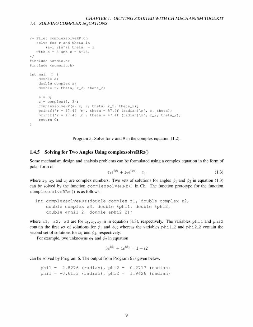
1.4.5 Solving for Two Angles Using complexsolveRRz()
Some mechanism design and analysis problems can be formulated using a complex equation in the form of
polar form of
z1eiφ1 + z2e
iφ2 = z3 (1.3)
where z1, z2, and z3 are complex numbers. Two sets of solutions for angles φ1 and φ2 in equation (1.3)
can be solved by the function complexsolveRRz() in Ch. The function prototype for the function
complexsolveRRz() is as follows:
int complexsolveRRz(double complex z1, double complex z2,
double complex z3, double &phi1, double &phi2,
double &phi1_2, double &phi2_2);
where z1, z2, z3 are for z1, z2, z3 in in equation (1.3), respectively. The variables phi1 and phi2
contain the first set of solutions for φ1 and φ2; whereas the variables phi1 2 and phi2 2 contain the
second set of solutions for φ1 and φ2, respectively.
For example, two unknowns φ1 and φ2 in equation
3eiφ1 + 4eiφ2 = 1 + i2
can be solved by Program 6. The output from Program 6 is given below.
phi1 = 2.8276 (radian), phi2 = 0.2717 (radian)
phi1 = -0.6133 (radian), phi2 = 1.9426 (radian)
9

1.4. SOLVING COMPLEX EQUATIONSCHAPTER 1. GETTING STARTED WITH CH MECHANISM TOOLKIT
/* solve for phi1 and phi2 in
z1 eˆ(i phi1) + z2 eˆ(i phi2) = z3
with z1 = 3, z2 = 4, z3 = 1+i2.
*/
#include <stdio.h>
#include <numeric.h>
int main () {
double complex z1, z2, z3;
double phi1, phi2, phi1_2, phi2_2;
z1 = complex(3, 0);
z2 = complex(4, 0);
z3 = complex(1, 2);
complexsolveRRz(z1, z2, z3, phi1, phi2, phi1_2, phi2_2);
printf("phi1 = %7.4f (radian), phi2 = %7.4f (radian)\n", phi1, phi2);
printf("phi1 = %7.4f (radian), phi2 = %7.4f (radian)\n", phi1_2, phi2_2);
return 0;
}
Program 6: Solve for φ1 and φ2 in the complex equation (1.3).
10

Chapter 2
Fourbar Linkage
The four-bar linkage, as shown in Figure 2.1, is the simplest closed-loop linkage. This section will describe
how to perform kinematic and dynamic analysis of four-bar linkages using the Ch Mechanism Toolkit.
2.1 Position Analysis
For the four-bar linkage shown in Figure 2.1, the displacement analysis can be formulated by the following
loop-closure equation
r2 + r3 = r1 + r4. (2.1)
Using complex numbers, equation (2.1) becomes
r2eiθ2 + r3e
iθ3 = r1eiθ1 + r4e
iθ4 , (2.2)
where link lengths r1, r2, r3, and r4 and angular position θ1 for the ground link are constants. Angle θ2 for
the input link is an independent variable; angles θ3 and θ4 for the coupler and output links, respectively, are
dependent variables. Equation (2.2) can be rearranged as
r3eiθ3 − r4e
iθ4 = r1eiθ1 − r2e
iθ2 . (2.3)
Let R1 = r3, φ1 = θ3, R2 = −r4, φ2 = θ4, z = (x3, y3) = r1eiθ1 − r2e
iθ2 , equation (2.3) becomes the
following general complex equation
R1eiφ1 +R2e
iφ2 = z. (2.4)
Given link lengths of a four-bar linkage and angles θ1 and θ2, the angular positions θ3 and θ4 can be solved
using function complexsolveRR() described in section 1.4. In general, there are two sets of solutions
for θ3 and θ4 for a given θ2, which correspond to two different circuits or two geometric inversions of a
circuit of the four-bar linkage [2]. A Non-Grashof linkage has one circuit with two geometric inversions. A
Grashof Crank-Rocker or Crank-Crank linkage has two circuits, each having only one geometric inversion.
However, a Grashof Rocker-Crank or Rocker-Rocker linkage has two circuits, each with two geometric
inversions.
Once the joint angle for θ3 is obtained, the position of coupler point P shown in Figure 2.1 can be
obtained. The position vector P for coupler point P can be expressed in vector form using complex numbers
as:
P = r2eiθ2 + rpe
i(θ3+β) (2.5)
A complex number z = (x, y) = reiθ in Ch can be constructed either by complex(x,y) or
polar(r,theta). Equation (2.5) can be translated into a Ch programming statement
11

2.1. POSITION ANALYSISCHAPTER 2. FOURBAR LINKAGE
Figure 2.1: The four-bar linkage.
P = polar(r2,theta2) + polar(rp,theta3+beta).
Using class CFourbar, a four-bar linkage analysis problem can be solved conveniently, which can be
illustrated by the following analysis problem.
Problem 1: Link lengths of a four-bar linkage, as shown in Figure 2.1, are given as follows:
r1 = 12cm, r2 = 4cm, r3 = 12cm, r4 = 7cm. The phase angle for the ground link is θ1 = 10◦,
the coupler point P is defined by the distance rp = 5cm and constant angle β = 20◦. Find the
angular positions θ3 and θ4 and the position for coupler point P when the input angle θ2 is 70◦.
Display the current position of the fourbar mechanism.
The four-bar linkage given in Problem 1 is a crank-rocker. There are two distinct circuits for each input
link position. The class CFourbar can be used to solve the analysis and design problems related to the four-
bar linkage as shown in Program 7. Two sets of solutions for angles θ3 and θ4 as well as the position vector
for coupler point P are calculated by the member functions angularPos() and couplerPointPos(),
respectively. Arrays in Ch are fully ISO C compatible, they are pointers. For consistency with text de-
scription, we use arrays with index starting with 1, instead of 0, in the mechanism toolkit. The output of
Program 7 is shown below:
theta3 = 0.459, theta4 = 1.527, P = complex( 4.822, 7.374) cm
theta3 = -0.777, theta4 = -1.845, P = complex( 5.917, 1.684) cm
Member function displayPosition() is called to graphically display the current position of the
fourbar linkage. It is prototyped as follows,
int CFourbar::displayPosition(double theta2, double theta3,
double theta4, ...
/*[int outputtype [, char *filename]]*/);
12

2.1. POSITION ANALYSISCHAPTER 2. FOURBAR LINKAGE
/* File: program1.ch */
#include <math.h>
#include <fourbar.h>
int main() {
CFourbar fourbar;
double r1 = 0.12, r2 = 0.04, r3 =0.12, r4 = 0.07,
theta1 = 10*M_PI/180;
double rp = 0.05, beta = 20*M_PI/180;
double theta_1[1:4], theta_2[1:4];
double complex p1, p2; // two solution of coupler point P
double theta2 = 70*M_PI/180;
theta_1[1] = theta1;
theta_1[2] = theta2; // theta2
theta_2[1] = theta1;
theta_2[2] = theta2; // theta2
fourbar.uscUnit(false);
fourbar.setLinks(r1, r2, r3, r4, theta1);
fourbar.setCouplerPoint(rp, beta);
fourbar.angularPos(theta_1, theta_2, FOURBAR_LINK2);
fourbar.couplerPointPos(theta2, p1, p2);
fourbar.displayPosition(theta2, theta_1[3], theta_1[4]);
fourbar.displayPosition(theta2, theta_2[3], theta_2[4]);
/**** the first set of solutions ****/
printf("theta3 = %6.3f, theta4 = %6.3f, P = %6.3f cm\n",
theta_1[3], theta_1[4], p1*100);
/**** the second set of solutions ****/
printf("theta3 = %6.3f, theta4 = %6.3f, P = %6.3f cm\n",
theta_2[3], theta_2[4], p2*100);
}
Program 7: Program for computing θ3, θ4 and position of the coupler point P of a four-bar linkage using
class CFourbar.
13

2.1. POSITION ANALYSISCHAPTER 2. FOURBAR LINKAGE
Figure 2.2: Current positions of the fourbar linkage.
where theta2,theta3, and theta4 are the current angular positions. It utilizes the QuickAnimationTM
program qanimate to display the fourbar mechanism. QuickAnimationTM will be discussed in further
detail in Chapter 7. Two optional arguments may be inputted into member function displayPosition()
after argument theta4. The value of the first optional argument may be either macro
QANIMATE OUTPUTTYPE DISPLAY, QANIMATE OUTPUTTYPE FILE, and
QANIMATE OUTPUTTYPE STREAM. Macro QANIMATE OUTPUTTYPE DISPLAY displays the fourbar
figure on the computer terminal, whereas macro QANIMATE OUTPUTTYPE STREAM sends the
qanimate data to the standard output stream. With macro QANIMATE OUTPUTTYPE FILE, the
qanimate data can be saved to a file with file name specified by the second optional input argument. The
default output value is QANIMATE OUTPUTTYPE DISPLAY. Figure 2.2 shows the current position for
both kinematic inversions of the fourbar linkage described in Problem 1. Note that fourbar linkage analysis
can be performed in either SI of US Customary units with class CFourbar. Member function uscUnit()
is called prior to any of the other member functions to specify whether US Customary units are desired. The
function prototype for member function uscUnit() is as follows,
void CFourbar::uscUnit(bool unit);
where the value of argument unit is either false or true. If unit is true, then the input and output values
are assumed to be in US Customary units. In this case, the length, time, force, and mass shall be specified in
foot, second, pound, and slug (lb− sec2/ft), respectively. If the value of unit is false, then the default
SI units are assumed. In this case, the length, time, force, and mass shall be specified in meter, second,
Newton, and kilogram, respectively. For example, the lengths, r1 to r4 for the linkage in Program 7 are
specified in meter.
Problem 2: Link lengths of a four-bar linkage, as shown in Figure 2.1, are given as follows:
r1 = 4.72in, r2 = 1.57in, r3 = 4.72in, r4 = 2.76in. The phase angle for the ground link
is θ1 = 10o, the coupler point P is defined by the distance rp = 1.97in and constant angle
β = 20o. Find the angular positions θ3 and θ4 and the position for coupler point P when the
input angle θ2 is 70o.
14

2.1. POSITION ANALYSISCHAPTER 2. FOURBAR LINKAGE
/* File: program2.ch */
#include <math.h>
#include <fourbar.h>
int main() {
CFourbar fourbar;
double r1 = 4.72/12.0, r2 = 1.57/12.0, r3 = 4.72/12.0, r4 = 2.76/12.0,
theta1 = 10*M_PI/180;
double rp = 1.97/12.0, beta = 20*M_PI/180;
double theta_1[1:4], theta_2[1:4];
double complex p1, p2; // two solution of coupler point P
double theta2 = 70*M_PI/180;
theta_1[1] = theta1;
theta_1[2] = theta2; // theta2
theta_2[1] = theta1;
theta_2[2] = theta2; // theta2
fourbar.uscUnit(true);
fourbar.setLinks(r1, r2, r3, r4, theta1);
fourbar.setCouplerPoint(rp, beta);
fourbar.angularPos(theta_1, theta_2, FOURBAR_LINK2);
fourbar.couplerPointPos(theta2, p1, p2);
/**** the first set of solutions ****/
printf("theta3 = %6.3f, theta4 = %6.3f, P = %6.3f in\n",
theta_1[3], theta_1[4], p1*12.0);
/**** the second set of solutions ****/
printf("theta3 = %6.3f, theta4 = %6.3f, P = %6.3f in\n",
theta_2[3], theta_2[4], p2*12.0);
}
Program 8: Program for computing θ3, θ4 and position of the coupler point P of a four-bar linkage using
US Customary units.
As another example, consider Problem 2 above, which requires the use of US Customary units for anal-
ysis. Problem 2 is similar to Problem 1, except that the link lengths are specified in inches rather than
centimeters. The solution to this problem is Program 8. In this program, the link lengths are converted from
inches to the desired unit of feet by multiplying a coefficient of 112 . In contrast to Program 7, the argument
of member function uscUnit() is true to indicate that US Customary units are desired for the results of
the fourbar analysis. The output of Program 8 is as follows:
theta3 = 0.462, theta4 = 1.529, P = complex( 1.894, 2.903) in
theta3 = -0.778, theta4 = -1.845, P = complex( 2.329, 0.656) in
Alternatively, fuunction complexsolveRR() can be used to solve the analysis and design problems
related to the four-bar linkage as shown in Program 7. Problem 1 can be solved by using Program 9. Two
sets of solutions for angles θ3 and θ4 as well as the position vector for coupler point P are calculated by
Program 9. The numerical output from Programs 7 and 9 are the same. Note that since Program 9 does not
use class CFourbar to solve Problem 1, the link dimensions may be specified in centimeters rather than
meters. However, the value for the coupler point position is in centimeters as well.
According to the IEEE 754 standard for binary floating-point arithmetic, any invalid solution in Ch
is symbolically represented as NaN. This can be very useful for analysis of mechanisms. For example,
15

2.1. POSITION ANALYSISCHAPTER 2. FOURBAR LINKAGE
/* File: fourbarTheta3Theta4P.ch */
#include <numeric.h>
int main() {
double r[1:4], theta[1:4], rp, beta;
double complex z, P;
double x1, x2, x3, x4;
/* specification of the four-bar linkage */
r[1] = 12; r[2] = 4; r[3] = 12; r[4] = 7; rp = 5; beta = 20*M_PI/180;
theta[1] = 10*M_PI/180; theta[2]=70*M_PI/180;
z = polar(r[1], theta[1]) - polar(r[2], theta[2]); /* z = r1-r2 */
complexsolveRR(r[3], -r[4], z, x1, x2, x3, x4);
/**** the first set of solutions ****/
theta[3] = x1; theta[4] = x2;
P = polar(r[2], theta[2]) + polar(rp, theta[3]+beta); /* P=r2+rp */
printf("theta3 = %6.3f, theta4 = %6.3f, P = %6.3f \n", theta[3], theta[4], P);
/**** the second set of solutions ****/
theta[3] = x3; theta[4] = x4;
P = polar(r[2], theta[2]) + polar(rp, theta[3]+beta); /* P=r2+rp */
printf("theta3 = %6.3f, theta4 = %6.3f, P = %6.3f \n", theta[3], theta[4], P);
}
Program 9: Program for computing θ3, θ4 and position of the coupler point P of a four-bar linkage.
if the link dimensions for the four-bar linkage in Problem 1 are changed to r1 = 12cm, r2 = 12cm, r3 =4cm, r4 = 7cm. The linkage then becomes a double-rocker. There are two circuits, each with two geometric
inversions, for this linkage. The input ranges for two separate circuits are 24.36◦ < θ2 < 64.56◦ and
315.44◦ < θ2 < 355.64◦. When the input angle θ2 is set to 70◦, there exist no solutions for θ3 and θ4 . This
can be gracefully handled in a Ch program. If the following programming statement
r[1] = 12; r[2] = 4; r[3] = 12; r[4] = 7;
in Program 9 is changed to
r[1] = 12; r[2] = 12; r[3] = 4; r[4] = 7;
the output from the program becomes
theta3 = NaN, theta4 = NaN, P = complex(NaN,NaN)
theta3 = NaN, theta4 = NaN, P = complex(NaN, NaN)
For motion analysis of a crank-rocker mechanism using Program 10, the output range of the rocker is
within 0 ∼ 2π. For this mechanism, the output may be as shown on the top part in Figure 2.3. There is a
jump when θ4 is π, because θ4 = π and θ4 = −π are the same point for the crank-rocker mechanism. If the
unwrap() function is used, a smooth curve for output angle θ4 can be obtained as shown on the lower part
in Figure 2.3.
Function unwrap() with the prototype of
int unwrap(array double &y, array double &x, ...
/* [double cutoff] */);
in the header file numeric.h unwraps the radian phase of each element of input array x by changing
its absolute jump greater than π to its 2π complement. The input array x can be of a vector or a two-
dimensional array. If it is a two-dimensional array, the function unwraps it through every row of the array.
Array argument y is the same dimension and size as x. It contains the unwrapped data. Optional argument
cutoff specifies the jump value. If the user does not specify this input, cutoff has a value of π by default.
16

2.1. POSITION ANALYSISCHAPTER 2. FOURBAR LINKAGE
/* File: unwrap.ch */
#include <numeric.h>
#include <chplot.h>
int main(){
double r[1:4],theta1,theta31;
int i;
double complex z,p,rb;
double x1,x2,x3,x4;
array double theta2[36],theta4[36],theta41[36];
CPlot subplot, *plot;
/* four-bar linkage*/
r[1]=5; r[2]=1.5; r[3]=3.5; r[4]=4;
theta1=30*M_PI/180;
linspace(theta2,0,2*M_PI);
for (i=0;i<36;i++) {
z=polar(r[1],theta1)-polar(r[2],theta2[i]);
complexsolveRR(r[3],-r[4],z,x1,x2,x3,x4);
theta4[i] = x2;
}
unwrap(theta41, theta4);
subplot.subplot(2,1);
plot = subplot.getSubplot(0,0);
plot->data2D(theta2, theta4);
plot->title("Wrapped");
plot->label(PLOT_AXIS_X,"Crank input: radians");
plot->label(PLOT_AXIS_Y,"Rocker output: radians");
plot = subplot.getSubplot(1,0);
plot->data2D(theta2, theta41);
plot->title("Unwrapped");
plot->label(PLOT_AXIS_X,"Crank input: radians");
plot->label(PLOT_AXIS_Y,"Rocker output: radians");
subplot.plotting();
}
Program 10: A program using unwrap().
17

2.1. POSITION ANALYSISCHAPTER 2. FOURBAR LINKAGE
-4
-3
-2
-1
0
1
2
3
4
0 1 2 3 4 5 6 7
Roc
ker
outp
ut: r
adia
ns
Crank input: radians
Wrapped
2.5
2.6
2.7
2.8
2.9
3
3.1
3.2
3.3
0 1 2 3 4 5 6 7
Roc
ker
outp
ut: r
adia
ns
Crank input: radians
Unwrapped
Figure 2.3: Comparison of results with and without using unwrap() function.
Function unwrap returns 0 on success and -1 on failure. The details about this function can be found in the
Ch Reference Guide.
A four-bar linkage may take form of a crank-rocker, double-crank (drag-link), double-rocker, or triple-
rocker [2]. Given the link dimensions and ground link, the type of the four-bar linkage can be determined
by Grashof criteria. The number of circuits and number of geometric inversions as well as the input and
output ranges for a given four-bar linkage can be determined. All these information can be determined by
member functions grashof() and getJointLimits() in the fourbar class. The function prototype
for member function grashof() is as follow:
int CFourbar::grashof(string_t &name)
where name of string type indicates the grashof type. The function returns a number that corresponds to
the distinct grashof type for the given link dimensions. If the fourbar links cannot form a valid linkage,
the return value is -1. Otherwise, it return a macro number which distinct the grashof type. The function
prototype for getJointLimits() is:
int CFourbar::getJointLimits(double inputmin[2], inputmax[2],
double outputmin[2], outputmax[2]);
where inputmin and inputmax are the minimum and maximum values for the ranges of motion for
input link 2, and
outputmin and outputmax are the minimum and maximum values for the ranges of motion for output
link 4. How these functions in the linkage toolbox is used for mechanism design can be demonstrated by
the following mechanism design problem.
Problem 3: The link lengths of a four-bar linkage, as shown in Figure 2.1, are given as follows:
r1 = 12cm, r2 = 4cm, r3 = 12cm, r4 = 7cm. The phase angle for link 1 is θ1 = 10◦, the
coupler point P is defined by distance rp = 5cm and constant angle β = 20◦, Determine the
type, and input and output ranges of the four-bar linkage. Plot the coupler curve for coupler
point P = (xp, yp) when input link 2 is rotated from θ2min to θ2max.
18

2.2. TRANSMISSION ANGLE ANALYSISCHAPTER 2. FOURBAR LINKAGE
/* File: program3.ch */
#include <fourbar.h>
int main() {
CFourbar fourbar;
double r1 = 0.12, r2 = 0.04, r3 = 0.10,
r4= 0.07;//crank-rocker
double theta1 = 10*M_PI/180;
double rp = 0.05, beta = 20*M_PI/180;
string_t fourbartype;
fourbar.uscUnit(false);
fourbar.setLinks(r1, r2, r3, r4, theta1);
fourbar.setCouplerPoint(rp, beta);
fourbar.setNumPoints(50);
fourbar.grashof(fourbartype);
printf("Linkage type: %s\n", fourbartype);
fourbar.printJointLimits();
int branchnum = 1;
CPlot plot1, plot2;
fourbar.plotCouplerCurve(&plot1, branchnum);
branchnum++;
plot2.outputType(PLOT_OUTPUTTYPE_FILE, "postscript eps", "couplerCurve.eps");
fourbar.plotCouplerCurve(&plot2, branchnum);
}
Program 11: Program couplerCurve() for generating coupler curves of a four-bar linkage.
You can solve this problem by Program 11. The output of Program 11 is shown in Figure 2.4. Note that
member function grashof() internally calls getJointLimits() to determine the input/output ranges
of the fourbar, so that member function printJointLimits() can display these values. Coupler curve
plots may also be saved to a file. For Program 11, the coupler curve plot for the second branch of the fourbar
mechanism is saved into an encapsulted postscript file by the following statement.
plot2.outputType(PLOT_OUTPUTTYPE_FILE, "postscript eps",
"couplerCurve.eps");
Function outputType() is a member of class CPlot. The first argument is a macro specifying that the
output plot should be saved to a file, with file type specified by the second input argument. The third input
argument is the file name. Note that member function CPlot::outputType() should be called prior
to member function CFourbar::plotCouplerCurve() as well as similar plotting functions for class
CFourbar and other mechanism classes.
2.2 Transmission Angle Analysis
The transmission angle for the fourbar mechanism is shown in Figure 2.1 as the angle γ. It is defined as
the acute angle between the velocity difference vector VBA (velocity of point B relative to point A) and the
absolute velocity vector Vout of the output link (link 4). Since vector VBA will always be perpendicular to
link 3 and Vout will always be perpendicular to link 4 at the 3-4 connection point (point B), the transmission
angle γ can be determined by using the following formula.
19

2.2. TRANSMISSION ANGLE ANALYSISCHAPTER 2. FOURBAR LINKAGE
Linkage type: Crank-Rocker
Input Characteristics: Input 360 degree rotation
Output Range:
Circuit: 1 2
(deg) (deg)
Lower limit: 98.98 -149.15
Upper limit: 169.15 -78.98
0
0.01
0.02
0.03
0.04
0.05
0.06
0.07
0.08
-0.01 0 0.01 0.02 0.03 0.04 0.05 0.06
Py
(m)
Px (m)
Coupler curve
-0.03
-0.025
-0.02
-0.015
-0.01
-0.005
0
0.005
0.01
0.015
0.02
0.025
0 0.01 0.02 0.03 0.04 0.05 0.06 0.07 0.08 0.09
Py
(m)
Px (m)
Coupler curve
Figure 2.4: The output of Program 11.
20

2.3. VELOCITY ANALYSISCHAPTER 2. FOURBAR LINKAGE
γ = θ4 − θ3 (2.6)
The CFourbar class contains three member functions for transmission angle analysis: transAngle(),
transAngles() and plotTransAngles(). Member function transAngle() can be used to cal-
culate the transmission angle of a fourbar linkage given the angular position of either link 2, 3, or 4. Its
function prototype is shown below.
void CFourbar::transAngle(double &gamma1, &gamma2, double theta,
int theta_id);
Output arguments gamma1 and gamma2 stores the two possible solutions of the transmission angle. Argu-
ment theta is the angular position value of the link specified by theta id.
The other two member functions, transAngles() and plotTransAngles(), can be used for
analysis of the transmission angle over the entire range of motion of the fourbar mechanism. The function
prototypes for transAngles() and plotTransAngles() are as follows.
void CFourbar::transAngles(int branchnum, double theta2[:],
double gamma[:]);
void CFourbar::plotTransAngles(class CPlot *pl, int branchnum);
For member function transAngle(), branchnum indicates the branch of the fourbar, and theta2
and gamma are arrays for storing values of θ2 and γ, respectively. The values of theta2 contains equally
incremented values ranging from θ2,min to θ2,max. The corresponding transmission angle values are stored
in array gamma. Note that the array size of theta2 and gamma must be the same.
Since the transmission angle γ is dependent on the input angle, θ2, it is convenient to be able to generate
a plot of the transmission angle for the entire range of motion of the input link. Although the two sets of data
values for θ2 and γ obtained by calling member function transAngle() can be used for plotting, member
function plotTransAngles() can be easily called to accomplish the same goal. Its first argument pl
is an object of class CPlot used for plotting.
Problem 4: Link lengths of a four-bar linkage, as shown in Figure 2.1, are given as follows:
r1 = 12cm, r2 = 4cm, r3 = 12cm, r4 = 7cm. The phase angle for the ground link is
θ1 = 10o. Generate a plot of the transmission angle for the valid range of motion for the
fourbar linkage.
The simplest solution to Problem 4 is use class CFourbar to first specify the fourbar linkage parame-
ters, and then call member function plotTransAngles() to generate the desired plot. Figure 2.5 shows
the two possible transmission angle plots for the fourbar linkage described in the above problem state-
ment. The source code for generating these two plots is listed as Program 12. Note that member function
setNumPoints() is used to specify the number of data points to generate for the plots.
2.3 Velocity Analysis
The velocity analysis for a closed-loop linkage can be carried out from its loop-closure equation. For
example, taking the derivative of the loop-closure equation (2.3), we get the following velocity relation
ω3r3eiθ3 − ω4r4e
iθ4 = −ω2r2eiθ2 (2.7)
21

2.3. VELOCITY ANALYSISCHAPTER 2. FOURBAR LINKAGE
/* File: transAngle.ch */
#include <fourbar.h>
int main() {
CFourbar fourbar;
double r1 = 0.12, r2 = 0.04, r3 = 0.12, r4 = 0.07, theta1 = 10*M_PI/180;
int numpoints = 50;
CPlot plota, plotb;
fourbar.setLinks(r1, r2, r3, r4, theta1);
fourbar.setNumPoints(numpoints);
fourbar.plotTransAngles(&plota, 1);
fourbar.plotTransAngles(&plotb, 2);
}
Program 12: Program for plotting the transmission angle for the valid range of motion of the fourbar mech-
anism.
30
40
50
60
70
80
90
100
110
120
0 50 100 150 200 250 300 350 400
gam
ma
(deg
)
theta2 (deg)
Transmission Angle Plot
-120
-110
-100
-90
-80
-70
-60
-50
-40
-30
0 50 100 150 200 250 300 350 400
gam
ma
(deg
)
theta2 (deg)
Transmission Angle Plot
Figure 2.5: Transmission angle plots.
22

2.4. ACCELERATION ANALYSISCHAPTER 2. FOURBAR LINKAGE
for the four-bar linkage shown in Figure 2.1. Given values of r2, r3, r4, θ2, θ3, θ4 and ω2, we can readily use
the function complexsolvePP() to compute angular velocities ω3 and ω4 for coupler and output links,
respectively. We can also derive analytical solutions for ω3 and ω4. Multiplying equation (2.7) with e−iθ4 ,
equation (2.7) becomes
ω3r3ei(θ3−θ4) − ω4r4 = −ω2r2e
i(θ2−θ4) (2.8)
The imaginary part of equation (2.8) gives
ω3r3 sin(θ3 − θ4) = −ω2r2 sin(θ2 − θ4) (2.9)
Then
ω3 = −ω2r2 sin(θ4 − θ2)
r3 sin(θ4 − θ3)(2.10)
Computation of the angular velocity ω3 can be programmed in Ch as function files or they can use a
single line of code. For example, ω3 can be calculated in foubar class using a member function named
angularVel().
Similarly, the following analytical expression for ω4 can be derived by multiplying equation (2.7) with
e−iθ3 ,
ω4 =ω2r2 sin(θ3 − θ2)
r4 sin(θ3 − θ4)(2.11)
ω4 also can be calculated in Ch using the fourbar class member function angularVel().
The derivative of equation (2.5) gives the following analytical expression for the velocity of coupler
point P .
Vp = iω2r2eiθ2 + iω3rpe
i(θ3+β) (2.12)
which can be translated into a Ch code fragment as
double r2, r3, theta2, theta3, rp, beta, omega2, omega3;
double complex I=complex(0,1), Vp;
Vp = I*omega2*polar(r2, theta2) + I*polar(omega3*rp, theta3+beta);
2.4 Acceleration Analysis
For a closed-loop planar linkage, the acceleration relation can be obtained by taking the second derivative of
the loop-closure equation. For example, by taking the second derivative of the loop-closure equation (2.3),
we get the following acceleration relation for the four-bar linkage shown in Figure 2.1.
iα3r3eiθ3 − ω2
3r3eiθ3 − iα4r4e
iθ4 + ω24r4e
iθ4 = iα2r2eiθ2 + ω2
2r2eiθ2 (2.13)
where α2, α3, and α4 are angular accelerations for input, coupler, and output links, respectively, Similar to
the derivation for ω3, the following analytical formulas for α3 and α4, respectively, can be derived:
α3 =−r2α2 sin(θ4 − θ2) + r2ω
22 cos(θ4 − θ2) + r3ω
23 cos(θ4 − θ3)− r4ω
24
r3 sin(θ4 − θ3)(2.14)
α4 =r2α2 sin(θ3 − θ2)− r2ω
22 cos(θ3 − θ2) + r4ω
24 cos(θ3 − θ4)− r3ω
23
r4 sin(θ3 − θ4)(2.15)
A fourbar class member function angularAccel() has been written for calculating α3 and α4. It is
included in the Ch Mechanism Toolkit.
23

2.5. DYNAMICSCHAPTER 2. FOURBAR LINKAGE
Figure 2.6: The four-bar linkage with offset gravity centers for moving links.
Figure 2.7: Free body diagrams for the moving links of the four-bar linkage.
2.5 Dynamics
The purpose of acceleration analysis is for inertia-force analysis. Given position, velocity, acceleration, and
inertia properties such as mass and mass moment of inertia for each moving link of a four-bar linkage, we are
able to perform force analysis for the linkage. Various formulations are available for dynamics. The matrix
method has been used in the formulation of the Ch Mechanism Toolkit [2]. To simplify the programming
burden, we have implemented computational arrays in the Ch programming language. Computational arrays
can be treated as single objects.
For the four-bar linkage shown in Figure 2.6, dynamic formulations can be derived to calculate the
required input torque Ts and joint reaction forces. Three free-body diagrams for links 2, 3, and 4 are given
in Figure 2.7. Three static equilibrium equations, in terms of forces in X and Y directions and moment about
the center of gravity of the link, can be written for each link.
24

2.5. DYNAMICSCHAPTER 2. FOURBAR LINKAGE
For link 2, we get
F12x + F32x + Fg2x = 0 (2.16)
−m2g + F12y + F32y + Fg2y = 0 (2.17)
Ts + (−rg2)× F12 + (r2 − rg2)× F32 + Tg2 = 0 (2.18)
where rg2 = rg2ei(θ2+δ2) is the position vector from joint A0 to the center of gravity of link 2. F12 and F32
are the joint forces acting on link 2 from the ground and link 3, respectively. Fg2 and Tg2 are the inertia
force and inertia moment, respectively, of link 2. m2 is the mass of link 2. Ts is the driving torque.
For link 3, we get
F23x + F43x + Fg3x = 0 (2.19)
−m3g + F23y + F43y + Fg3y = 0 (2.20)
(−rg3)×F23 + (r3 − rg3)× F43 + Tg3 = 0 (2.21)
where rg3 = rg3ei(θ3+δ3) is the position vector from joint A to the center of gravity of link 3. F23 and F43
are the joint forces acting on link 3 from links 2 and 4, respectively. Fg3 and Tg3 are the inertia force and
inertia moment, respectively, of link 3. m3 is the mass of link 3.
For link 4, we get
F34x + F14x + Fg4x = 0 (2.22)
−m4g + F34y + F14y + Fg4y = 0 (2.23)
(−rg4)× F14 + (r4 − rg4)× F34 + Tg4 + Tl = 0 (2.24)
where rg4 = rg4ei(θ4+δ4) is the position vector from joint B0 to the center of gravity of link 4. F14 and F34
are the joint forces acting on link 4 from the ground and link 3, respectively. Fg4 and Tg4 are the inertia
force and inertia moment, respectively, of link 4. m4 is the mass of link 4. Tl is the torque of external load.
Equations (2.18), (2.21), and (2.24) can be expressed explicitly as
Ts − rg2 cos(θ2 + δ2)F12y + rg2 sin(θ2 + δ2)F12x
+[r2 cos θ2 − rg2 cos(θ2 + δ2)]F32y − [r2 sin θ2 − rg2 sin(θ2 + δ2)]F32x + Tg2 = 0 (2.25)
−rg3 cos(θ3 + δ3)F23y + rg3 sin(θ3 + δ3)F23x
+[r3 cos θ3 − rg3 cos(θ3 + δ3)]F43y − [r3 sin θ3 − rg3 sin(θ3 + δ3)]F43x + Tg3 = 0 (2.26)
−rg4 cos(θ4 + δ4)F14y + rg4 sin(θ4 + δ4)F14x
+[r4 cos θ4 − rg4 cos(θ4 + δ4)]F34y − [r4 sin θ4 − rg4 sin(θ4 + δ4)]F34x + Tg4 + Tl = 0 (2.27)
Note that Fijx = −Fjix and Fijy = −Fjiy, equations (2.16-2.24) can be rewritten as nine linear equations in
terms of nine unknowns F12x, F12y , F23x, F23y, F34x, F34y , F14x, F14y , and Ts (8 joint reaction forces plus
one input torque). They can be expressed in a symbolic form
Ax = b (2.28)
where x = (F12x, F12y , F23x, F23y , F34x, F34y , F14x, F14y , Ts)T is a vector consisting of the unknown
forces and input torque, b = (Fg2x, Fg2y −m2g, Tg2 , Fg3x, Fg3y −m3g, Tg3 , Fg4x, Fg4y −m4g, Tg4 + Tl)T
is a vector that contains external load plus inertia forces and inertia torques, and A is a 9x9 square matrix
25

2.5. DYNAMICSCHAPTER 2. FOURBAR LINKAGE
A =
−1 0 1 00 −1 0 1
−rg2 sin(θ2 + δ2) rg2 cos(θ2 + δ2) rg2 sin(θ2 + δ2)− r2 sin θ2 r2 cos θ2 − rg2 cos(θ2 + δ2)0 0 −1 00 0 0 −10 0 −rg3 sin(θ3 + δ3) rg3 cos(θ3 + δ3)0 0 0 00 0 0 00 0 0 0
0 0 0 0 00 0 0 0 00 0 0 0 −11 0 0 0 00 1 0 0 0
rg3 sin(θ3 + δ3)− r3 sin θ3 r3 cos θ3 − rg3 cos(θ3 + δ3) 0 0 0−1 0 −1 0 00 −1 0 −1 0
r4 sin θ4 − rg4 sin(θ4 + δ4) rg4 cos(θ4 + δ4)− r4 cos θ4 −rg4 sin(θ4 + δ4) rg4 cos(θ4 + δ4) 0
(2.29)
formed using the angular position of each link and link parameters. What distinguish the above-derived
equations (2.16)-(2.24) from those in Erdman and Sandor [2] are that the center of gravity of each link is
not at the center line between two joints and the gravitation force for each link is included in formulations
explicitly. Because equation (2.28) has 9 unknowns, it should be solved numerically. This can be easily
implemented in Ch by only a single line of code shown below,
X = inverse(A)*B
A fourbar class member function force() has been written for the Ch Mechanism Toolkit. Function
force() can calculate the joint forces and required input torque to achieve the desired motion of the four-
bar linkage. The first three input arguments of the function force() are arrays, theta[i] for joint angle
θi, omega[i] for angular velocity ωi, alpha[i] for angular acceleration αi, tl is the external load
Tl. The output X from the function force() contains the joint forces and required input torque, which
is passed to the calling function as an argument of assumed-shape computational array. How to use this
function in the toolkit can be demonstrated by the following mechanism design problem given in [2].
Problem 5: Link parameters and inertia properties of a four-bar linkage, as shown in Figure 2.6,
are given in the chart below.
Length Weight Ig C. G.
Link r (in) (lb) (lbf ft sec2) rg (in) δ
1 12 — — — —
2 4 0.8 0.0010 2 0
3 12 2.4 0.0099 6 0
4 7 1.4 0.0032 3.5 0
The phase angle for link 1 is θ1 = 0. There is no external load. At one point the input
angular position θ2 = 150◦, angular velocity ω2 = 5 rad/sec ccw and angular acceleration
α2 = 5 rad/sec2 cw, find the joint reaction forces and required input torque at this moment.
26

2.5. DYNAMICSCHAPTER 2. FOURBAR LINKAGE
/* File: program4.ch */
#include <math.h>
#include <fourbar.h>
int main() {
CFourbar fourbar;
double r1 = 12/12.0, r2 = 4/12.0, r3 =12/12.0, r4 = 7/12.0, theta1 = 0;
double rp = 5/12.0, beta = 20*M_PI/180;
double theta_1[1:4], theta_2[1:4], omega[1:4], alpha[1:4];
array double X[9];
double g=32.2;
double rg2 = 2/12.0, rg3 = 6/12.0, rg4 = 3.5/12.0;
double delta2 = 0.0, delta3 = 0, delta4 = 0.0;
double m2 = 0.8/g, m3 = 2.4/g, m4 = 1.4/g;
double ig2 = 0.0010, ig3 = 0.0099, ig4 = 0.0032, tl=0;
/* initialization of link parameters and
inertia properties */
theta_1[1] = 0; theta_1[2]=150*M_PI/180;
theta_2[1] = 0; theta_2[2]=150*M_PI/180;
omega[2] = 5; alpha[2] = -5;
fourbar.uscUnit(true);
fourbar.setLinks(r1, r2, r3, r4, theta1);
fourbar.setCouplerPoint(rp, beta);
fourbar.setGravityCenter(rg2, rg3, rg4, delta2, delta3, delta4);
fourbar.setInertia(ig2, ig3, ig4);
fourbar.setMass(m2, m3, m4);
// find theta3, theta4
fourbar.angularPos(theta_1, theta_2, FOURBAR_LINK2);
// find omega3, omega4, first set
fourbar.angularVel(theta_1, omega, FOURBAR_LINK2);
// find alpha3, alpha4
fourbar.angularAccel(theta_1, omega, alpha, FOURBAR_LINK2);
// find forces, torque
fourbar.forceTorque(theta_1, omega, alpha, tl, X);
printf("first solution X = %.4f \n", X);
// find omega3, omega4, second set
fourbar.angularVel(theta_2, omega, FOURBAR_LINK2);
// find alpha3, alpha4
fourbar.angularAccel(theta_2, omega, alpha, FOURBAR_LINK2);
// find forces, torque
fourbar.forceTorque(theta_2, omega, alpha, tl, X);
printf("second solution X = %.4f \n", X);
}
Program 13: Program force() for computing joint reaction forces and required input torque.
27

2.6. KINEMATICS AND DYNAMICS WITH CONSTANT ANGULAR VELOCITY FOR LINK 2CHAPTER 2. FOURBAR LINKAGE
You can solve this problem by Program 13. Note that the various lengths, masses, and moments of inertia
are represented in feet, slugs, and lb−ft−sec2, respectively. The output of Program 13 is given as follows:
first solution X = 1.7993 2.3553 1.6993 1.5895 1.1643 -0.7428 -1.0273 2.1624 -0.8659
second solution X = -0.6161 2.4778 -0.7161 1.7120 -1.1555 -0.4193 1.2368 1.7218 -0.4987
Problem 6: Link parameters and inertia properties of a four-bar linkage are given in the chart
below.
Length Mass Ig C. G.
Link r (cm) (kg) (kg m2) rg (cm) δ
1 30.48 — — — —
2 10.16 0.3628 0.001356 5.08 0
3 30.48 1.0883 0.013445 15.24 0
4 17.78 0.6348 0.004293 8.89 0
The phase angle for link 1 is θ1 = 0. There is no external load. At one point the input
angular position θ2 = 150◦, angular velocity ω2 = 5 rad/sec ccw and angular acceleration
α2 = 5 rad/sec2 cw, find the joint reaction forces and required input torque at this moment.
Program 14 is the equivalent of Program 13, except that SI units are used rather than US Customary
units. The output of Program 14 is shown below. Note that this output is the SI equivalent to the output for
Program 13.
first solution X = 8.0075 10.4824 7.5624 7.0739 5.1815 -3.3056 -4.5716 9.6234 -1.1746
second solution X = -2.7421 11.0279 -3.1873 7.6194 -5.1427 -1.8663 5.5045 7.6627 -0.6765
2.6 Kinematics and Dynamics with Constant Angular Velocity for Link 2
Analysis of the fourbar mechanism described in the previous sections were performed for only one specific
position. Assuming constant angular velocity for the input link, link 2, this section will discuss analysis
of the fourbar linkage over the entire range of motion of this link. With constant angular velocity, the
relationships between the angular position, velocity, and acceleration for link 2 is as follows,
θ2 = ω0t+ θ2,min
ω2 = ω0
α2 = 0
where θ2,min is the minimum angular position value of the link, and ω0 is a constant value. Note that the
total time for one rotation of the input link, θ2 = θ2,min to θ2 = θ2,max, can be determined by the following
equation,
tmax =θ2,max − θ2,min
ω0
28

2.6. KINEMATICS AND DYNAMICS WITH CONSTANT ANGULAR VELOCITY FOR LINK 2CHAPTER 2. FOURBAR LINKAGE
/* File: program5.ch */
#include <math.h>
#include <fourbar.h>
int main() {
CFourbar fourbar;
double r1 = 0.3048, r2 = 0.1016, r3 = 0.3048, r4 = 0.1778,
theta1 = 0;
double rp = 0.1270, beta = 20*M_PI/180;
double theta_1[1:4], theta_2[1:4], omega[1:4], alpha[1:4];
array double X[9];
double g = 9.81;
double rg2 = 0.0508, rg3 = 0.1524, rg4 = 0.0889;
double delta2 = 0.0, delta3 = 0, delta4 = 0.0;
double m2 = 0.3628, m3 = 1.0883, m4 = 0.6348;
double ig2 = 0.001356, ig3 = 0.013445, ig4 = 0.004293, tl=0;
/* initialization of link parameters and
inertia properties */
theta_1[1] = 0; theta_1[2]=150*M_PI/180;
theta_2[1] = 0; theta_2[2]=150*M_PI/180;
omega[2] = 5; alpha[2] = -5;
fourbar.uscUnit(false);
fourbar.setLinks(r1, r2, r3, r4, theta1);
fourbar.setCouplerPoint(rp, beta);
fourbar.setGravityCenter(rg2, rg3, rg4, delta2, delta3, delta4);
fourbar.setInertia(ig2, ig3, ig4);
fourbar.setMass(m2, m3, m4);
// find theta3, theta4
fourbar.angularPos(theta_1, theta_2, FOURBAR_LINK2);
// find omega3, omega4, first set
fourbar.angularVel(theta_1, omega, FOURBAR_LINK2);
// find alpha3, alpha4
fourbar.angularAccel(theta_1, omega, alpha, FOURBAR_LINK2);
// find forces, torque
fourbar.forceTorque(theta_1, omega, alpha, tl, X);
printf("first solution X = %.4f \n", X);
// find omega3, omega4, second set
fourbar.angularVel(theta_2, omega, FOURBAR_LINK2);
// find alpha3, alpha4
fourbar.angularAccel(theta_2, omega, alpha, FOURBAR_LINK2);
// find forces, torque
fourbar.forceTorque(theta_2, omega, alpha, tl, X);
printf("second solution X = %.4f \n", X);
}
Program 14: Program force() for computing joint reaction forces and required input torque in SI units.
29

2.6. KINEMATICS AND DYNAMICS WITH CONSTANT ANGULAR VELOCITY FOR LINK 2CHAPTER 2. FOURBAR LINKAGE
/* File: constangvel.ch */
#include <math.h>
#include <stdio.h>
#include <fourbar.h>
int main() {
double r[1:4], theta1;
double omega2;
int numpoints = 50;
CFourbar fourbar;
CPlot plota, plotb, plotc;
/* default specification of the four-bar linkage */
r[1] = 12; r[2] = 4; r[3] = 12; r[4] = 7;
theta1 = 10*M_PI/180;
omega2 = 5; /* rad/sec */
fourbar.setLinks(r[1], r[2], r[3], r[4], theta1);
fourbar.setAngularVel(omega2);
fourbar.setNumPoints(numpoints);
fourbar.plotAngularPoss(&plota, 1);
fourbar.plotAngularVels(&plotb, 1);
fourbar.plotAngularAccels(&plotc, 1);
return 0;
}
Program 15: Program for plotting θ3, θ4, ω3, ω4, α3, and α4 with respect to time.
where θ2,max is the maximum angular position value for link 2.
Using the above relationships, member functions plotAngularPos(),plotAngularVel(), and
plotAngularAccel() of class CFourbar were developed for time-based kinematic analysis of links
3 and 4 of a fourbar mechanism . Given a constant value for ω2, these member functions can be used to
plot the angular positions, velocities, and accelerations of links 3 and 4 with respect to time. The function
prototypes for these member functions are as follows.
void CFourbar::plotAngularPoss(class CPlot *pl, int branchnum);
void CFourbar::plotAngularVels(class CPlot *pl, int branchnum);
void CFourbar::plotAngularAccels(class CPlot *pl, int branchnum);
Argument pl is an object of class CPlotused for plotting, and branchnum is the branch number of the
fourbar linkage to analyze.
Problem 7: Link lengths of a four-bar linkage, as shown in Figure 2.1, are given as follows:
r1 = 12cm, r2 = 4cm, r3 = 12cm, r4 = 7cm. The phase angle for the ground link is
θ1 = 10o, and the constant angular velocity of the input link is ω2 = 5rad/sec. Plot the
angular positions, velocities, and accelerations of links 3 and 4 with respect to time for the 1st
branch.
The solution to Problem 7 is Program 15. After specifying the required parameters for the fourbar class,
member functions plotAngularPoss(), plotAngularVels(), and plotAngularAccels()
are called to generate the desired plots. The outputs of Program 15 are Figures 2.8 - 2.10.
30

2.6. KINEMATICS AND DYNAMICS WITH CONSTANT ANGULAR VELOCITY FOR LINK 2CHAPTER 2. FOURBAR LINKAGE
20
40
60
80
100
120
140
160
0 0.2 0.4 0.6 0.8 1 1.2 1.4
thet
a (d
eg)
time (sec)
Angular Position Plots
theta3theta4
Figure 2.8: Angular position plot.
-250
-200
-150
-100
-50
0
50
100
150
200
0 0.2 0.4 0.6 0.8 1 1.2 1.4
omeg
a (d
eg/s
ec)
time (sec)
Angular Velocity Plots
omega3omega4
Figure 2.9: Angular velocity plot.
31

2.6. KINEMATICS AND DYNAMICS WITH CONSTANT ANGULAR VELOCITY FOR LINK 2CHAPTER 2. FOURBAR LINKAGE
-1000
-500
0
500
1000
1500
2000
0 0.2 0.4 0.6 0.8 1 1.2 1.4
alph
a (d
eg/s
ec^2
)
time (sec)
Angular Acceleration Plots
alpha3alpha4
Figure 2.10: Angular acceleration plot.
In addition to member functions plotAngularPoss(), plotAngularVels(), and
plotAngularAccels(), memeber functions angularPoss(), angularVels(), and
angularAccels() are also available for kinematic analysis of the fourbar linkage with constant an-
gular velocity for link 2. Instead of generating plots of the angular position, velocity, and acceleration
of links 3 and 4 as with the plotting functions described above, these other functions generates the data
used for plotting and store them into arrays for later use. For, example the generated data can be saved
to a data file or used to generate plots similar to plotAngularPoss(), plotAngularVels(), and
plotAngularAccels(). These functions have the following function prototypes.
int CFourbar::angularPoss(int branchnum, double time[:],
double theta3[:], double theta4[:]);
int CFourbar::angularVels(int branchnum, double time[:],
double omega3[:], double omega4[:]);
int CFourbar::angularAccels(int branchnum, double time[:],
double alpha3[:], double alpha4[:]);
Argument branchnum is an integer value specifying the branch of the fourbar. Array time is a set of
time values equally incremented from time t = 0 to t = tmax, where tmax is the total time required
for one complete motion of the fourbar. Arrays theta3, theta4, omega3, omega4, alpha3, and
alpha4 contains corresponding values for the angular positions, velocities, and accelerations of links 3
and 4, respectively. Note that the array arguments for the above member functions should all have the same
size.
For dynamic analysis of the fourbar linkage with a constant ω2 value, member functions forceTorques()
and plotForceTorques() are available. Member function forceTorques() determines the joint
forces and input torque for the entire valid range of motion of the fourbar mechanism, whereas
plotForceTorques() generates a graphical representation of these values. Their function prototypes
are as follows.
int CFourbar::forceTorques(int branchnum, double tl, array double time[:],
f12x[:], f12y[:], f23x[:], f23y[:],
32

2.6. KINEMATICS AND DYNAMICS WITH CONSTANT ANGULAR VELOCITY FOR LINK 2CHAPTER 2. FOURBAR LINKAGE
/*************************************************************
* File: forceTorques.ch
* This example plots the joint forces and output torque curves.
**************************************************************/
#include <math.h>
#include <fourbar.h>
int main()
{
CFourbar fourbar;
double r1 = 0.12, r2 = 0.04, r3 = 0.10, r4= 0.07;
double theta1 = 10;
double rg2 = 0.0508, rg3 = 0.1524, rg4 = 0.0889;
double delta2 = 0.0, delta3 = 0, delta4 = 0.0;
double m2 = 0.3628, m3 = 1.0833, m4 = 0.6348;
double ig2 = 0.001356, ig3 = 0.013445, ig4 = 0.004293, tl=0;
int numpoint = 50;
double omega2 = 5; /* constant omega2 */
CPlot plot;
/* initialization of link parameters and
inertia properties */
fourbar.uscUnit(true);
fourbar.setLinks(r1, r2, r3, r4, theta1);
fourbar.setGravityCenter(rg2, rg3, rg4, delta2, delta3, delta4);
fourbar.setInertia(ig2, ig3, ig4);
fourbar.setMass(m2, m3, m4);
fourbar.setNumPoints(numpoint);
fourbar.setAngularVel(omega2);
fourbar.plotForceTorques(&plot,1,tl); //first branch
}
Program 16: Program for plotting joint forces and output torque with respect to time.
f34x[:], f34y[:], f14x[:], f14y[:], ts[:]);
int CFourbar::plotForceTorques(class CPlot *pl, int branchnum,
double tl);
For these functions, tl is the load torque, time is an array to record time, and f12x, f12y, f23x, f23y,
f34x, f34y, f14x, f14y, and ts are arrays for the joint forces and input torque.
Problem 8: Link lengths of a four-bar linkage, as shown in Figure 2.1, are given as follows:
r1 = 12cm, r2 = 4cm, r3 = 10cm, r4 = 7cm. The phase angle for the ground link is θ1 = 0,
the constant angular velocity of the input link is ω2 = 5rad/sec, and load torque tl = 0.
Using the inertia properties provided in the prevous problems for dynamic analysis, plot the
joint forces and input torque for the valid range of motion of the fourbar mechanism for the 1st
branch.
Program 16 is the solution to the above problem statement. After indicating the link parameters and
inertia properties, member function plotForceTorques() is called to generate the desired plot. The
plot of the joint forces and input torque is listed as Figure 2.11.
33

2.7. THREE-POSITION SYNTHESISCHAPTER 2. FOURBAR LINKAGE
-80
-60
-40
-20
0
20
40
60
80
100
0 0.2 0.4 0.6 0.8 1 1.2 1.4
forc
e (lb
f)/to
rque
(lb
f-ft)
time t (seconds)
F12_xF12_yF23_xF23_yF34_xF34_yF14_xF14_y
Ts
Figure 2.11: Joint forces and input torque plot.
2.7 Three-Position Synthesis
Recall the loop-closure equation for the fourbar linkage rewritten below.
r1 + r4 = r2 + r3 (2.30)
r1eiθ1 + r4e
iθ4 = r2eiθ2 + r3e
iθ3 (2.31)
Previously, equation (2.31) was used to derive equations for calculating the angular positions, velocities, and
accelerations of the remaining links given the dynamic properties of one link. Similarly, the loop-closure
equation provides a basis for the synthesis of fourbar mechanisms given three sets of input/output angles.
Assuming θ1 = 0, equation (2.31) is rewritten as equations (2.32) and (2.33). The next step is to eliminate
θ3 in the equations, which can be done by first isolating the terms containing θ3 on the right-hand side.
r1 + r4 cos θ4 = r2 cos θ2 + r3 cos θ3 (2.32)
r4 sin θ4 = r2 cos θ2 + r3 cos θ3 (2.33)
r1 + r4 cos θ4 − r2 cos θ2 = r3 cos θ3 (2.34)
r4 sin θ4 − r2 sin θ2 = r3 sin θ3 (2.35)
Squaring and adding equations (2.34) and (2.35) together will then cancel out the θ3 term, which results in
equation (2.37),
r23 − r21 − r22 − r242r2r4
+r1r4
cos θ2 −r1r2
cos θ4 = − cos θ2 − θ4 (2.36)
k1 cos θ2 + k2 cos θ4 + k3 = − cos θ2 − θ4 (2.37)
where
k1 =r1r4
34

2.7. THREE-POSITION SYNTHESISCHAPTER 2. FOURBAR LINKAGE
k2 =−r1r2
k3 =r23 − r21 − r22 − r24
2r2r4.
Equation 2.37 is called Freudenstein’s equation.
φφ
φψ
ψψ
12
3
12
3
Figure 2.12: Freudenstein analysis.
The three unknowns in equation (2.37), k1, k2, and k3, can be solved for three-point function generation.
Thus, for three prescribed positions as shown in Figure 2.12, Freudenstein’s equation becomes,
k1 cosφ1 + k2 cosφ1 + k3 = − cosφ1 − ψ1 (2.38)
k1 cosφ2 + k2 cosφ2 + k3 = − cosφ2 − ψ2 (2.39)
k1 cosφ3 + k2 cosφ3 + k3 = − cosφ3 − ψ3 (2.40)
which can be simplified into Ax = b or equation (2.41).
cos(φ1) cos(ψ1) 1cos(φ2) cos(ψ2) 1cos(φ3) cos(ψ3) 1
k1k2k3
=
− cos(φ1 − ψ1)− cos(φ2 − ψ2)− cos(φ3 − ψ3)
(2.41)
Once the values for k1, k2, and k3 are obtained from equation (2.41, link dimensions r2, r3, and r4 can be
solved in terms of input link length r1 with equations (2.42) - (2.44). Typically, the length r1 is chosen to be
1.
r4 =r1k1
(2.42)
r2 =−r1k2
(2.43)
r3 =√
2k3r2r4 + r21 + r22 + r24 (2.44)
Class CFourbar also contains member function synthesis() to calculate the various link lenths
using Freudenstein’s equation. The function prototype for synthesis() is shown below.
int CFourbar::synthesis(double r[1:4], double phi[:], double psi[:]);
35

2.8. ANIMATIONCHAPTER 2. FOURBAR LINKAGE
Argument r is a 4-element array to store the values of the link lengths. Note that element r[1] shall be
a given value, and elements r[2], r[3], and r[4] shall contain the outputs of the function. Arguments
phi and psi are used to specify the sets of input and output angles, respectively.
Problem 9: Given r1 = 1m, φ = [105o, 157o, 209o], and ψ = [66.27o, 102.42o, 119.67o],calculate the link lengths r2, r3, and r4. Also display the fourbar linkage at the three specified
positions.
Problem 9 can be solved by using member function synthesis() described above and another mem-
ber function displayPositions(), which is similar to member function displayPosition() de-
scribed in Section 2.1. Its function prototype is as follows,
int CFourbar::displayPositions(double theta2[:], double theta3[:],
double theta4[:], ...
/*[int outputtype [, char *filename]]*/);
It is similar to member function displayPosition(), except that multiple positions may be displayed
in one figure. Arguments theta2, theta3, and theta4 shall have the same number of elements, and
the arrays’ argument size shall specify the number of positions to display.
The solution to Problem 9 is Program 17. After specifying the length of the ground link r1 and the
three sets of input/output angles, member function synthesis() is called to determine link dimensions
r2, r3, and r4. Next, the three θ3 values are calculated by using member function getAngle(). It has the
following function prototype,
int CFourbar::getAngle(double theta[1:], int theta_id);
where theta are the angular position values and theta id indicates the unknown link angle. Mem-
ber function setLinks() is then called to define the fourbar linkage in order to use member function
displayPositions() to display the fourbar mechanism in the three specified positions. The output of
Program 17 is shown in Figure 2.13.
2.8 Animation
The concepts discussed in Section 2.1 concerning position analysis of a fourbar linkage can be applied to
simulate the motion of a fourbar mechanism. By applying the Grashof criteria or calling member function
grashof(), the type of fourbar as well as the number of geometric inversions can be determined. Fur-
thermore, the range of the input link, link 2, can also be calculated by hand or by using member function
getJointLimits(), which is invoked internally when calling member function grashof(). With the
range of the input link known, the angular positions of the other links can be determined by applying the
equations developed in Section 2.1 for any instance of link 2. Thus, a for-loop can be utilized to obtain the
positions of links 3 and 4 for the entire range of the input link.
Utilizing the above observations, member function animation()was designed to simulate the motion
of a fourbar linkage. Its function prototype is as follows,
int CFourbar::animation(int branchnum, ...);
where branchnum indicates the branch number of the fourbar to simulate. For typical fourbar linkages,
branchnum can be either 1 or 2 for the first and second geometric inversions, respectively. However, for
36
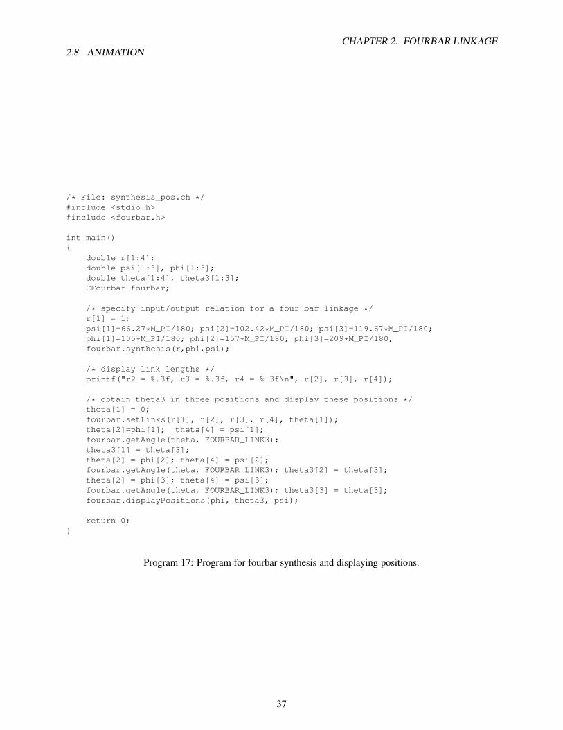
2.8. ANIMATIONCHAPTER 2. FOURBAR LINKAGE
/* File: synthesis_pos.ch */
#include <stdio.h>
#include <fourbar.h>
int main()
{
double r[1:4];
double psi[1:3], phi[1:3];
double theta[1:4], theta3[1:3];
CFourbar fourbar;
/* specify input/output relation for a four-bar linkage */
r[1] = 1;
psi[1]=66.27*M_PI/180; psi[2]=102.42*M_PI/180; psi[3]=119.67*M_PI/180;
phi[1]=105*M_PI/180; phi[2]=157*M_PI/180; phi[3]=209*M_PI/180;
fourbar.synthesis(r,phi,psi);
/* display link lengths */
printf("r2 = %.3f, r3 = %.3f, r4 = %.3f\n", r[2], r[3], r[4]);
/* obtain theta3 in three positions and display these positions */
theta[1] = 0;
fourbar.setLinks(r[1], r[2], r[3], r[4], theta[1]);
theta[2]=phi[1]; theta[4] = psi[1];
fourbar.getAngle(theta, FOURBAR_LINK3);
theta3[1] = theta[3];
theta[2] = phi[2]; theta[4] = psi[2];
fourbar.getAngle(theta, FOURBAR_LINK3); theta3[2] = theta[3];
theta[2] = phi[3]; theta[4] = psi[3];
fourbar.getAngle(theta, FOURBAR_LINK3); theta3[3] = theta[3];
fourbar.displayPositions(phi, theta3, psi);
return 0;
}
Program 17: Program for fourbar synthesis and displaying positions.
37

2.8. ANIMATIONCHAPTER 2. FOURBAR LINKAGE
r2 = 0.555, r3 = 1.441, r4 = 0.725
Figure 2.13: The output of Program 17.
a rocker-rocker mechanism, branchnum can have a maximum value of 4 for the four possible branches of
the rocker-rocker mechanism.
Additionally, member function animation() supports the option to store the data used for the gen-
erating the fourbar animation into a file. This file can be used by the Quick Animation program to simulate
the movement of the fourbar linkage at another time. The format for saving data to a file is shown below.
fourbar.animation(branchnum, QANIMATE_OUTPUTTYPE_FILE, "data.qnm");
Macro QANIMATE OUTPUTTYPE FILE specifies that the data to be generated by the animation()
function is to be stored into file "data.qnm", where .qnm is the file extension for the Quick Animation
program. A more in depth discussion of Quick Animation will be given in Chapter 7.
In order to simulate movement of the fourbar linkage, the number of frames to generate needs to be spec-
ified. This can be done by member function setNumPoints(), which is also used to specify the number
of data points to plot the coupler and force/torque curves with member functions plotCouplerCurve()
and plotForceTorques(). As an example, consider the crank-rocker mechanism described in Prob-
lem 3. Program 18 can be used to simulate the motion for each branch of this linkage. Figure 2.14 represents
the output of Program 18, which consists of two frames from the two geometric inversions of the fourbar
linkage in Problem 3. The third argument of member function setCouplerPoint() is an optional argu-
ment to indicate whether or not the coupler curve should be traced in the animation. This argument may be
either macro TRACE ON or TRACE OFF. For the case of Program 18, tracing of the coupler curve in the an-
imation is desired. by default, the tracing is turned off. Note that if the fourbar is a Grashof Rocker-Rocker,
there would exist a total of four branches, since a Rocker-Rocker mechanism has four possible input ranges.
If this is true, then the following code fragment would simulate the motion of the third and fourth branch
of the fourbar linkage. However, if a third or fourth branch is specified, and the fourbar is not a Grashof
Rocker-Rocker, then an error would occur.
fourbar.animation(3);
fourbar.animation(4);
38

2.8. ANIMATIONCHAPTER 2. FOURBAR LINKAGE
/* File: program3_ani.ch */
#include <fourbar.h>
int main() {
CFourbar fourbar;
double r1 = 0.12, r2 = 0.04, r3 = 0.10,
r4= 0.07; //crank-rocker
double theta1 = 10*M_PI/180;
double rp = 0.05, beta = 20*M_PI/180;
string_t fourbartype;
fourbar.uscUnit(false);
fourbar.setLinks(r1, r2, r3, r4, theta1);
fourbar.setCouplerPoint(rp, beta, TRACE_ON);
fourbar.setNumPoints(50);
fourbar.animation(1);
fourbar.animation(2);
}
Program 18: Program for simulating the motion of a fourbar linkage.
Figure 2.14: The animation from Program 18.
39

2.9. WEB-BASED FOURBAR LINKAGE ANALYSISCHAPTER 2. FOURBAR LINKAGE
2.9 Web-Based Fourbar Linkage Analysis
Fourbar linkage analysis can also be done through the World Wide Web. Web pages have been specifically
designed to perform the same types of analysis discussed in previous sections. The main web page for
mechanism design and analysis through the internet is shown as Figures 2.15. This web page contain links
to other web pages that include descriptions and examples of special fourbar linkages as well as links to web
pages to perform fourbar linkage analysis and synthesis.
2.9.1 Position Analysis
As an example of using the fourbar linkage analysis web pages, recall the problem statement of Problem 1
in Section 2.1. Given all the necessary link lenghts, r1 to r4, and angles θ1 and θ2, the problem asked
for the values of θ3 and θ4. This problem can easily be solved with the ”Interactive Four-Bar Linkage
Position Analysis” web page and corresponding Ch script, which can be directed by the ”Position Analysis”
link under the ”Four-Bar Linkage Analysis” section shown in Figure 2.15. The web page designed for
calculating θ3 and θ4 as well as the vector representing the coupler point position is shown in Figure 2.16.
The derivation of the analytical solution of θ3 and θ4 are provided in the first section of the page. The second
section allows the user to input data required for performing the position analysis. In this section, the user
can input the link lengths, θ1, and coupler point parameters rp and β. Note that angles θ1 and β can be
specified in either degrees or radians with the Degree Mode/Radian Mode tab. Furthermore, given any
known angle (θ2, θ3, θ4), this web page can be used to calculate the value of the two remaining angles. For
this example, r1 = 12cm, r2 = 4cm, r3 = 12cm, r4 = 7cm, rp = 5cm, θ1 = 10o, θ2 = 70o, and β = 20o.
After all the parameters have been entered, the user can click on the ”Run” button to execute the Ch script
for calculating θ3 and θ4 as well as the coupler point position. Output of the analysis are displayed directly
on the web page, which is shown Figure 2.17. Note that the ”Reset” button resets all the inputted values to
their default values.
2.9.2 Coupler Curve Plotting
Plotting the coupler curve can be done by the internet web page shown in Figure 2.18. All the user need
to do is input the values for the link lengths, θ1, and coupler point parameters, rp and β. Once all the
values have been entered, the user can click on the ”Run” button to plot the coupler curve for the specified
fourbar linkage. For example, using the parameters specified in Problem 2, the coupler curve plot for the
first geometric inversion is shown as Figure 2.19.
2.9.3 Animation
Figure 2.20 shows the web page that allows users to simulate the motion of a fourbar mechanism via the
internet. Like all the other web pages previously mentioned, the user can click on the ”Run” button after
inputting on the required parameters to generate the animation. Note that the number frames and branch
number may be indicated in their specified locations. Using the fourbar specifications of Problem 2, a frame
of the animation obtained from the web page is shown in Figure 2.21.
40

2.9. WEB-BASED FOURBAR LINKAGE ANALYSISCHAPTER 2. FOURBAR LINKAGE
Figure 2.15: Main web page for fourbar linkage analysis and synthesis.
41

2.9. WEB-BASED FOURBAR LINKAGE ANALYSISCHAPTER 2. FOURBAR LINKAGE
Figure 2.16: Web page for fourbar linkage position analysis.
42

2.9. WEB-BASED FOURBAR LINKAGE ANALYSISCHAPTER 2. FOURBAR LINKAGE
Figure 2.16: Web page for fourbar linkage position analysis (Contd.).
Figure 2.17: Output of fourbar linkage position analysis.
43

2.9. WEB-BASED FOURBAR LINKAGE ANALYSISCHAPTER 2. FOURBAR LINKAGE
Figure 2.18: Web page for coupler curve plotting.
44

2.9. WEB-BASED FOURBAR LINKAGE ANALYSISCHAPTER 2. FOURBAR LINKAGE
Figure 2.19: Coupler curve plot.
45

2.9. WEB-BASED FOURBAR LINKAGE ANALYSISCHAPTER 2. FOURBAR LINKAGE
Figure 2.20: Web page for fourbar animation.
46

2.9. WEB-BASED FOURBAR LINKAGE ANALYSISCHAPTER 2. FOURBAR LINKAGE
Figure 2.21: Fourbar animation.
47

Chapter 3
Crank-Slider Mechanism
For a crank-slider mechanism shown in Figure 3.1, the displacement R1 for the slider has constant angle and
variable length. the crank R2, has constant length and variable angle as does R3, often called the connecting
rod. The offset R4 for slider has constant length and angle. It is the variation in the length of R1 that causes
the translational motion. The offset R4 can be positive or negative. In most applications, the offset is zero.
The angle θ4 is related to θ1 as θ4 = θ1 + 90◦.
Often an intermediate type of motion between the pure rotation of the crank and the pure translation of
the slider is desired. This can be obtained at P , the coupler point, which is offset from link 3 by a constant
length and angle.
Figure 3.1: A crank-slider mechanism.
In order to have 360◦ rotation for the crank link, the length of link 3 shall be greater than link 2 and
the difference of the link lengths for links 3 and 2 shall be greater than the offset. That is r3 > r2 and
r3 − r2 > r4. If r2 is greater than r3, the limiting configuration shown in Figure 3.2 will be reached. The
value of θ2 at this limiting configuratoin is
θ2lim =
[
θ1 + sin−1(
r3 + r4r2
)]
(3.1)
48

3.1. POSITION ANALYSISCHAPTER 3. CRANK-SLIDER MECHANISM
Figure 3.2: A limiting position for a crank-slider mechanism for r2 > r3.
Figure 3.3: A limiting position for a crank-slider mechanism for r3 − r2 < r4.
If r3 − r2 < r4, a limiting configuration shown in Figure 3.3 will be reached. The value of θ2 for this
limiting configuration will be
θ2lim =
[
θ1 + sin−1(
r3 − r4r2
)]
(3.2)
If r2 + r3 = r4, no rotation is possible. If r2 + r3 > r4, the links cannot form a valid crank-slider
mechanism.
3.1 Position Analysis
Since the vectors describing the four links of the crank-slider mechanism form a complete loop, the describ-
ing equation is known as the loop equation. The loop equation is the foundation for the analysis of the four
bar linkage and its variations. The loop equation is
R2 +R3 = R1 +R4 (3.3)
A general vector R can be represented in complex polar with two parameters, a length r and an angle θ.
Thus each vector can be represented as
R = reiθ (3.4)
In complex polar form the loop equation becomes
r2eiθ2 + r3e
iθ3 = r1eiθ1 + r4e
iθ4 (3.5)
49

3.1. POSITION ANALYSISCHAPTER 3. CRANK-SLIDER MECHANISM
The first step in describing the motion of the crank slider is deriving the two unknown parameters as func-
tions of the known parameters. At this point θ1, θ2, θ4, r2, r3 and r4 are known. The unknown parameters
are r1 and θ3. Rearranging equation (3.5) so that the terms containing the unknown parameters are on the
left and the terms containing only known parameters are on the right gives
r1eiθ1 − r3e
iθ3 = r2eiθ2 − r4e
iθ4 (3.6)
Converting the right side into Cartesian form where
a = r2 cos θ2 − r4 cos θ4 (3.7)
and
b = r2 sin θ2 − r4 sin θ4 (3.8)
gives
r1eiθ1 − r3e
iθ3 = a+ ib (3.9)
Multiplying by e−iθ1 gives
r1 − r3ei(θ3−θ1) = e−iθ1(a+ ib) (3.10)
and equating the imaginary parts of both sides eliminates r1 and produces
−r3 sin(θ3 − θ1) = a sin(−θ1) + b cos(−θ1) (3.11)
Solving for θ3 yields two solutions below.
θ3 = θ1 + sin−1(
a sin θ1 − b cos θ1r3
)
(3.12)
θ3 = θ1 + π − sin−1(
a sin θ1 − b cos θ1r3
)
(3.13)
Equating the real parts of equation (3.9) gives
r1 cos θ1 − r3 cos θ3 = a (3.14)
and solving for r1 gives
r1 =a+ r3 cos θ3
cos θ1(3.15)
The slider position is determined by
R1 +R4 (3.16)
r1eiθ1 + r4e
iθ1+90◦ (3.17)
The x and y components of the slider position are the real and imaginary parts of equation(3.17).
The joint angle θ3 and slider position r1 can be determined by using member functions angularPos()
and sliderPos() of class CCrankSlider, respectively. The following problem illustrates how class
CCrankSlider can be used to calculate these two values.
Problem 1: For the crank-slider mechanism shown in Figure 3.1, if r2 = 1cm, r3 = 5cm, r4 =0.5cm, and θ1 = 10o, find the displacement r1 of the slider and the joint angle θ3 when θ2 =45o. Display the current position of the crank-slider mechanism.
50
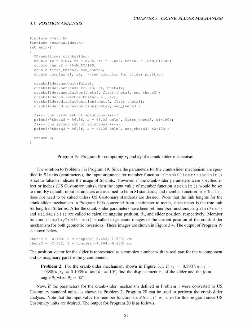
3.1. POSITION ANALYSISCHAPTER 3. CRANK-SLIDER MECHANISM
#include <math.h>
#include <crankslider.h>
int main()
{
CCrankSlider crankslider;
double r2 = 0.01, r3 = 0.05, r4 = 0.005, theta1 = 10*M_PI/180;
double theta2 = 45*M_PI/180;
double first_theta3, sec_theta3;
double complex s1, s2; //two solution for slider position
crankslider.uscUnit(false);
crankslider.setLinks(r2, r3, r4, theta1);
crankslider.angularPos(theta2, first_theta3, sec_theta3);
crankslider.sliderPos(theta2, s1, s2);
crankslider.displayPosition(theta2, first_theta3);
crankslider.displayPosition(theta2, sec_theta3);
/**** the first set of solutions ****/
printf("theta3 = %6.3f, S = %6.3f cm\n", first_theta3, s1*100);
/**** the second set of solutions ****/
printf("theta3 = %6.3f, S = %6.3f cm\n", sec_theta3, s2*100);
return 0;
}
Program 19: Program for computing r1 and θ3 of a crank-slider mechanism.
The solution to Problem 1 is Program 19. Since the parameters for the crank-slider mechanism are spec-
ified in SI units (centimeters), the input argument for member function CCrankSlider::uscUnit()
is set to false to indicate the usage of SI units. However, if the crank-slider parameters were specified in
feet or inches (US Customary units), then the input value of member function uscUnit() would be set
to true. By default, input parameters are assumed to be in SI standards, and member function uscUnit()
does not need to be called unless US Customary standards are desired. Note that the link lenghts for the
crank-slider mechanism in Program 19 is converted from centimeter to meter, since meter is the true unit
for length in SI terms. After the crank-slider parameters have been set, member functions angularPos()
and sliderPos() are called to calculate angular position, θ3, and slider position, respectively. Member
function displayPosition() is called to generate images of the current position of the crank-slider
mechanism for both geometric inversions. These images are shown in Figure 3.4. The output of Program 19
is shown below.
theta3 = 0.160, S = complex( 5.643, 1.503) cm
theta3 = -2.952, S = complex(-4.204,-0.233) cm
The position vector for the slider is represented as a complex number with its real part for the x-component
and its imaginary part for the y-component.
Problem 2: For the crank-slider mechanism shown in Figure 3.1, if r2 = 0.3937in, r3 =1.9685in, r4 = 0.1969in, and θ1 = 10o, find the displacement r1 of the slider and the joint
angle θ3 when θ2 = 45o.
Now, if the parameters for the crank-slider mechanism defined in Problem 1 were converted to US
Customary standard units, as shown in Problem 2, Program 20 can be used to perform the crank-slider
analysis. Note that the input value for member function uscUnit() is true for this program since US
Customary units are desired. The output for Program 20 is as follows.
51

3.1. POSITION ANALYSISCHAPTER 3. CRANK-SLIDER MECHANISM
Figure 3.4: Current positions of the crank-slider mechanism.
#include <math.h>
#include <crankslider.h>
int main()
{
CCrankSlider crankslider;
double r2 = 0.3937/12.0, r3 = 1.9685/12.0, r4 = 0.1969/12.0,
theta1 = 10*M_PI/180;
double theta2 = 45*M_PI/180;
double first_theta3, sec_theta3;
double complex s1, s2; //two solution for slider position
crankslider.uscUnit(true);
crankslider.setLinks(r2, r3, r4, theta1);
crankslider.angularPos(theta2, first_theta3, sec_theta3);
crankslider.sliderPos(theta2, s1, s2);
/**** the first set of solutions ****/
printf("theta3 = %6.3f, S = %6.3f in\n", first_theta3, s1*12);
/**** the second set of solutions ****/
printf("theta3 = %6.3f, S = %6.3f in\n", sec_theta3, s2*12);
return 0;
}
Program 20: Program for computing r1 and θ3 of a crank-slider mechanism in US Customary standard.
52

3.2. TRANSMISSION ANGLESCHAPTER 3. CRANK-SLIDER MECHANISM
Figure 3.5: Transmission angle for a crank-slider mechanism.
theta3 = 0.160, S = complex( 2.222, 0.592) in
theta3 = -2.952, S = complex(-1.655,-0.092) in
3.2 Transmission Angles
The transmission angle, γ, is a measure of how effectively force is transmitted to the output link. When γis 90◦ all of the force is transmitted to the output link and when γ is 0 no force is transmitted to the output
link. In the crank-slider there are two transmission angles; one where the slider is the output link and one
where the crank is the output link as shown in Figure 3.5.
If the slider is the output, the transmission angle γ1 can be obtained by
γ1 = 90◦ − (θ3 − θ1) (3.18)
γ1 = 90◦ + θ1 − θ3 (3.19)
If the crank is the output, the transmission angle γ2 can be obtained by
γ2 = (θ2 − θ1) + (θ3 − θ1) (3.20)
γ2 = θ2 + θ3 − 2θ1 (3.21)
The transmission angles can be computed by the member function transAngle(), whose prototype is as
follow:
void CCrankSlider::transAngle(double &gamma1, &gamma2, double theta2);
where the first two arguments are the first and second solution to the transmission angle and argument
theta2 is the angular position of link 2.
3.3 Velocity Analysis
The angular and translational velocities are the rates at which the positions of the links change with respect
to time.
53

3.3. VELOCITY ANALYSISCHAPTER 3. CRANK-SLIDER MECHANISM
Figure 3.6: Velocities for a crank-slider mechanism.
Beginning with the complex loop equation (3.5), the velocities can be derived by first taking the derivative
with respect to time.d
dt(r2e
iθ2 + r3eiθ3) =
d
dt(r1e
iθ1 + r4eiθ4) (3.22)
r2eiθ2 + iθ2r2e
iθ2 + r3eiθ3 + iθ3r3e
iθ3 = r1eiθ1 + iθ1r1e
iθ1 + r4eiθ4 + iθ4r4e
iθ4 (3.23)
For the crank-slider the parameters r2, r3, r4, θ1 and θ4 are constant, thus
r2 = r3 = r4 = 0 and θ1 = θ4 = 0
By definition
θ2 ≡ ω2 , θ3 ≡ ω3 and r1 ≡ v1
Thus upon substitution into equation (3.23), we obtain
V1 = v1eiθ1 = iω2r2e
iθ2 + iω3r3eiθ3 (3.24)
This is the vector describing the velocity of link 1, the slider. In order to find the scalar values ω3 and v1first multiply both sides by e−iθ1 to produce
v1 = iω2r2ei(θ2−θ1) + iω3r3e
i(θ3−θ1) (3.25)
Equating the imaginary parts of both sides in equation (3.25) and solving for ω3 gives
ω3 =−ω2r2 cos(θ2 − θ1)
r3 cos(θ3 − θ1)(3.26)
The x component of velocity of the slider is the real part of equation (3.24).
vx = ω2 sin θ2 + ω3 sin θ3 (3.27)
The y component of velocity of the slider is the imaginary part of equation (3.24).
vy = ω2 cos θ2 + ω3 cos θ3 (3.28)
54

3.4. ACCELERATION ANALYSISCHAPTER 3. CRANK-SLIDER MECHANISM
Figure 3.7: Accelerations for a crank-slider mechanism.
The absolute magnitude of V1 is the real part of equation (3.25).
|v1| = ω2r2 sin(θ2 − θ1) + ω3r3 sin(θ3 − θ1) (3.29)
The angular and linear velocities can also be computed by member functions angularVel() and
sliderVel(), respectively.
3.4 Acceleration Analysis
The accelerations of the links is the rate at which their velocities change with respect with time.
The accelerations are derived by taking the derivative with respect to time of the velocity vector V1, equation
(3.24).d
dtV1 =
d
dtv1e
iθ1 =d
dt(iω2r2e
iθ2 + iω3eiθ3) (3.30)
v1eiθ1 + iθ1v1e
iθ1 = iω2r2eiθ2 + iω2r2e
iθ2 + i2θ2ω2r2eiθ2 + iω3r3e
iθ3 + iω3r3eiθ3 + i2ω3r3e
iθ3 (3.31)
By definition
v1 ≡ a1, ω2 ≡ α2, ω3 ≡ α3 and i2 ≡ −1
Substituting these and the previously defined values gives
A1 = a1eiθ1 = iα2r2e
iθ2 − ω22r2e
iθ + iα3r3eiθ3 − ω2
3r3eiθ3 (3.32)
Multiplying equation (3.32) by e−iθ1 yields
a1 = iα2r2ei(θ2−θ1) − ω2
2r2ei(θ2−θ1) + iα3r3e
i(θ3−θ1) − ω23r3e
i(θ3−θ1) (3.33)
Equating the imaginary parts of equation (3.33) and solving for α3 gives
α3 =ω22r2 sin(θ2 − θ1) + ω2
3r3 sin(θ3 − θ1)− α2r2 cos(θ2 − θ1)
r3 cos(θ3 − θ1)(3.34)
55

3.5. POSITION, VELOCITY AND ACCELERATION OF COUPLER POINTCHAPTER 3. CRANK-SLIDER MECHANISM
Figure 3.8: Coupler Point of a crank-slider mechanism.
The real part of equation (3.32) gives the x component of the slider acceleration.
ax = α2r2 sin θ2 − ω22r2 cos θ2 + α3r3 sin θ3 − ω2
3r3 cos θ3 (3.35)
The imaginary part of equation (3.32) gives the y component of the slider acceleration.
ay = α2r2 cos θ2 − ω22r2 sin θ2 + α3r3 cos θ3 − ω2
3r3 sin θ3 (3.36)
The real part of equation (3.33) gives the absolute magnitude of the slider acceleration.
|a1| = α2r2 sin(θ2 − θ1)− ω22r2 cos(θ2 − θ1) + α3r3 sin(θ3 − θ1)− ω2
3r3 cos(θ3 − θ1) (3.37)
Similar to velocity analysis, the angular and linear accelerations are computed by member functions
angularAccel() and sliderAccel(), respectively.
3.5 Position, Velocity and Acceleration of Coupler Point
The motion of the coupler point is related to that of link 3. Its angle with respect to ground is that of link 3
plus a constant β.
θ5 = θ3 + β (3.38)
The vector P represents the location of the coupler point.
P = R2 +R5 = r2eiθ2 + r5e
i(θ3+β) (3.39)
The x coordinate of P is
px = r2 cos θ2 + r5 cos(θ3 + β) (3.40)
and the y coordinate is
py = r2 sin θ2 + r5 sin(θ3 + β) (3.41)
The time derivative of P gives the velocity vector Vp.
Vp =d
dtP = iω2r2e
iθ2 + iω3r5ei(θ3+β) (3.42)
56

3.6. DYNAMIC FORCE ANALYSISCHAPTER 3. CRANK-SLIDER MECHANISM
The x coordinate of the coupler velocity is
vpx = ω2r2 sin θ2 + ω3r5 sin(θ3 + β) (3.43)
and the y coordinate is
vpy = ω2r2 cos θ2 + ω3r5 cos(θ3 + β) (3.44)
The time derivative of Vp gives the acceleration vector Ap.
Ap =d
dtVp = iα2r2e
iθ2 − ω22r2e
iθ2 + iα3r5ei(θ3+β) − ω2
3r5ei(θ3+β) (3.45)
The x coordinate of the coupler acceleration is
apx = α2r2 sin θ2 − ω22r2 cos θ2 + α3r5 sin(θ3 + β)− ω2
3r5 cos(θ3 + β) (3.46)
and the y coordinate is
apy = α2r2 cos θ2 − ω22r2 sin θ2 + α3r5 cos(θ3 + β)− ω2
3r5 sin(θ3 + β) (3.47)
The position, velocity, and acceleration of a coupler point can be computed by the following member func-
tions: couplerPointPos(), couplerPointVel(), couplerPointAccel(), respectively. For
example, the following problem may be solved with Program 21.
Problem 3: For a crank-slider mechanism with properties r2 = 1cm, r3 = 5cm, r4 = 0.5cm,
θ1 = 10o, rp = 2.5cm, and β = 20o, find the position, velocity, and acceleration of the coupler
point, P, when θ2 = 45o, ω2 = 5rad/sec, and α2 = 0.
The output of Program 21 is as follows:
Circuit 1:
Coupler Position: complex(2.669,2.257) cm
Coupler Velocity: complex(-2.266,1.929) cm/s
Coupler Acceleration: complex(-23.424,-13.111) cm/sˆ2
Circuit 2:
Coupler Position: complex(2.574,2.370) cm
Coupler Velocity: complex(-4.898,5.065) cm/s
Coupler Acceleration: complex(-0.142,-0.241) cm/sˆ2
3.6 Dynamic Force Analysis
Dynamic force analysis can be performed based on D’Alembert’s Principle – the sum of the inertial or body
forces and torques and the external forces and torques together produce equilibrium. This is analogous to
the criteria for static equilibrium as
∑
F = 0 and∑
M = 0
except that now the inertial or dynamic forces must be included in the sum.
The summations can be expressed as∑
F + (−mag) = 0 (3.48)
and∑
M + (−Iαg) = 0 (3.49)
57

3.6. DYNAMIC FORCE ANALYSISCHAPTER 3. CRANK-SLIDER MECHANISM
#include <math.h>
#include <crankslider.h>
int main() {
CCrankSlider crankslider;
double r2 = 0.01, r3 = 0.05, r4 = 0.005, theta1 = 10*M_PI/180;
double rp = 0.025, beta = 20*M_PI/180;
double theta2 = 45*M_PI/180;
double complex P[1:2], Vp[1:2], Ap[1:2];
double omega2 = 5; /* rad/sec */
double alpha2 = 0; /* rad/sec*sec */
double first_theta3, sec_theta3;
double first_omega3, sec_omega3;
double first_alpha3, sec_alpha3;
crankslider.setLinks(r2, r3, r4, theta1);
crankslider.setCouplerPoint(rp, beta);
crankslider.angularPos(theta2, first_theta3, sec_theta3);
crankslider.couplerPointPos(theta2, P[1], P[2]);
first_omega3 = crankslider.angularVel(theta2, first_theta3, omega2);
sec_omega3 = crankslider.angularVel(theta2, sec_theta3, omega2);
Vp[1] = crankslider.couplerPointVel(theta2, first_theta3,
omega2, first_omega3);
Vp[2] = crankslider.couplerPointVel(theta2, sec_theta3,
omega2, sec_omega3);
first_alpha3 = crankslider.angularAccel(theta2, omega2,
first_theta3, first_omega3, alpha2);
sec_alpha3 = crankslider.angularAccel(theta2, omega2,
sec_theta3, sec_omega3, alpha2);
Ap[1] = crankslider.couplerPointAccel(theta2, first_theta3, omega2,
first_omega3, alpha2,
first_alpha3);
Ap[2] = crankslider.couplerPointAccel(theta2, sec_theta3, omega2,
sec_omega3, alpha2,
sec_alpha3);
printf("Circuit 1:\n");
printf(" Coupler Position: %.3f cm\n", P[1]*100);
printf(" Coupler Velocity: %.3f cm/s\n", Vp[1]*100);
printf(" Coupler Acceleration: %.3f cm/sˆ2\n", Ap[1]*100);
printf("Circuit 2:\n");
printf(" Coupler Position: %.3f cm\n", P[2]*100);
printf(" Coupler Velocity: %.3f cm/s\n", Vp[2]*100);
printf(" Coupler Acceleration: %.3f cm/sˆ2\n", Ap[2])*100;
return 0;
}
Program 21: Program for computing the coupler point properties of a crank-slider mechanism.
58

3.6. DYNAMIC FORCE ANALYSISCHAPTER 3. CRANK-SLIDER MECHANISM
Figure 3.9: The free body diagram for link 2 of a crank-slider mechanism.
In dynamic analysis, we assume that the position, velocity and acceleration of each moving body in the sys-
tem are already known. The free body diagram for link 2 with all forces acting on it is shown in Figure 3.9.
The real part of the complex acceleration vector at the mass center, Ag, is the x component of accelera-
tion and the imaginary part is the y component.
Acceleration at the mass center can be obtained by
Ag2 =d2
dt2(Rg2) =
d2
dt2(rg2e
iθ2) (3.50)
Ag2 = iα2rg2eiθ2 − ω2
2rg2eiθ2 (3.51)
Based on the Newton’s second law, we can obtain the dynamic equation
Fg2x = m2Re(Ag2) (3.52)
Fg2y = m2Im(Ag2) (3.53)
Tg2 = I2α2 (3.54)
where m is the mass of the body and I is the mass moment of inertia about the mass center. The above
equation can be expanded as∑
Fx = F1,2x + F3,2x + Fg2x = 0 (3.55)
∑
Fy = F1,2y + F3,2y + Fg2y = −m2g = 0 (3.56)
∑
Mg = F1,2xrg2 sin θ2 − F1,2yrg2 cos θ2 − F3,2x(r2 − rg2) sin θ2
+F3,2y(r2 − rg2) cos θ2 + Tin − Tg2 = 0 (3.57)
The free body diagram for link 3 with all forces acting on it is shown in Figure 3.10. Acceleration at the
center of the mass for link 3 is
Ag3 =d2
dt2(R2 +Rg3) =
d2
dt2(r2e
iθ2 + rg3ei(θ3+φ)) (3.58)
Ag3 = iα2r2eiθ2 − ω2
2r2eiθ2 + iα3rg3e
i(θ3+φ) − ω23rg3e
i(θ3+φ) (3.59)
59

3.6. DYNAMIC FORCE ANALYSISCHAPTER 3. CRANK-SLIDER MECHANISM
Figure 3.10: The free body diagram for link 3 of a crank-slider mechanism.
The equations of motion
Fg3x = m3Re(Ag3) (3.60)
Fg3y = m3Im(Ag3) (3.61)
Tg3 = I3α3 (3.62)
The alternative equations of motion
∑
Fx = F2,3x + F4,3x + Fg3x = 0 (3.63)
∑
Fy = F2,3y + F4,3y + Fg3y −m3g = 0 (3.64)
∑
Mg = F2,3xrg3 sin(θ3 + φ)− F2,3yrg3 cos(θ3 + φ)− F4,3x [r3 sin θ3 − rg3 sin(θ3 + φ)]
+F3,4y [r3 cos θ3 − rg3 cos(θ3 + φ)]− Tg3 = 0 (3.65)
The free body diagram for link 4 with all forces acting on it is shown in Figure 3.11.
The acceleration at the center of the mass for the slider of link 4 is
Ag4 = A1 = iα2r2eiθ2 − ω2
2r2eiθ2 + iα3r3e
iθ3 − ω23r3e
iθ3 (3.66)
The equations of motion
Fg4x + Fl cos θ1 = m4Re(Ag4) (3.67)
Fg4y + Fl sin θ1 = m4Im(Ag4) (3.68)
Tg2 = 0 (3.69)
The alternative equations of motion
∑
Fx = F3,4x + F1,4x + Fg4x + Fl cos θ1 = 0 (3.70)
∑
Fy = F3,4y + F1,4y −m4g + Fg4y + Fl sin θ1 = 0 (3.71)
60

3.6. DYNAMIC FORCE ANALYSISCHAPTER 3. CRANK-SLIDER MECHANISM
Figure 3.11: The free body diagram for link 4 of a crank-slider mechanism.
Figure 3.12: The reaction forces on slider.
61

3.6. DYNAMIC FORCE ANALYSISCHAPTER 3. CRANK-SLIDER MECHANISM
There is no moment acting on link 4 as its motion is completely translational. The third equation necessary
to describe the forces acting on link 4 comes from the fact that F1,4x and F1,4y are components of a force
F1,4N that always acts normal to the ground as shown in Figure 3.12.
F1,4n cos θ1 = F1,4x (3.72)
−F1,4n sin θ1 = F1,4y (3.73)
F1,4x cos θ1 = F1,4y sin θ1 (3.74)
F1,4x cos θ1 + F1,4y sin θ1 = 0 (3.75)
Let F3,2 = −F2,3 and F4,3 = −F3,4, we can get the following system of equations.
Fg2x = −F1,2x + F2,3x
Fg2y −m2g = −F1,2y + F2,3y
−Tg2 = −[(r2 − rg2) sin θ2]F2,3x + [(r2 − rg2) cos θ2]F2,3y
−(rg2 sin θ2)F1,2x + (rg2 cos θ2)− Tin
Fg3x = −F2,3x + F3,4x
Fg3y −m3g = −F2,3y + F3,4y
−Tg3 = −[rg3 sin(θ3 + φ)]F2,3x + [rg3 cos(θ3 + φ)]F2,3y
−[r3 sin θ3 − rg3 sin(θ3 + φ)]F3,4x
+[r3 cos θ3 − rg3 cos(θ3 + φ)]F3,4y
Fg4x + Fl cos θ1 = −F3,4x − F1,4x
Fg4y −m4g + Fl sin θ1 = −F3,4y − F1,4y
0 = cos θ1F1,4x + sin θ1F1,4y
For the convenience of equation writing, let
a = −rg2 sin θ2b = rg2 cos θ2c = −(r2 − rg2) sin θ2d = (r2 − rg2) cos θ2e = −rg3 sin(θ3 + φ)
f = rg3 cos(θ3 + φ)g = −(r3 sin θ3 − rg3 sin(θ3 + φ))h = r3 cos θ3 − rg3 cos(θ3 + φ)i = cos θ1j = sin θ1
the system of equations in a matrix form can be obtained as follows.
Fg2xFg2y −m2g
−Tg2Fg3x
Fg3y −m3g
−Tg3Fg4x + Fl cos θ1
Fg4y −m4g + Fl sin θ10
=
−1 0 1 0 0 0 0 0 00 −1 0 1 0 0 0 0 0a b c d 0 0 0 0 −10 0 −1 0 1 0 0 0 00 0 0 −1 0 1 0 0 00 0 e f g h 0 0 00 0 0 0 −1 0 −1 0 00 0 0 0 0 −1 0 −1 00 0 0 0 0 0 i j 0
F1,2xF1,2y
F2,3xF2,3y
F3,4xF3,4y
F1,4xF1,4y
Tin
62
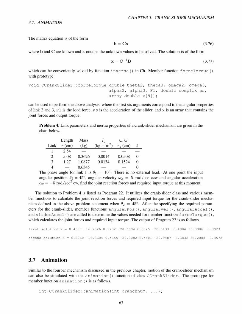
3.7. ANIMATIONCHAPTER 3. CRANK-SLIDER MECHANISM
The matrix equation is of the form
b = Cx (3.76)
where b and C are known and x ontains the unknown values to be solved. The solution is of the form
x = C−1
B (3.77)
which can be conveniently solved by function inverse() in Ch. Member function forceTorque()
with prototype
void CCrankSlider::forceTorque(double theta2, theta3, omega2, omega3,
alpha2, alpha3, Fl, double complex as,
array double x[9]);
can be used to perform the above analysis, where the first six arguments correspond to the angular properties
of link 2 and 3, Fl is the load force, as is the acceleration of the slider, and x is an array that contains the
joint forces and output torque.
Problem 4: Link parameters and inertia properties of a crank-slider mechanism are given in the
chart below.
Length Mass Ig C. G.
Link r (cm) (kg) (kg −m2) rg (cm) δ
1 2.54 — — — —
2 5.08 0.3626 0.0014 0.0508 0
3 1.27 1.0877 0.0134 0.1524 0
4 — 0.6345 — — 0
The phase angle for link 1 is θ1 = 10o. There is no external load. At one point the input
angular position θ2 = 45◦, angular velocity ω2 = 5 rad/sec ccw and angular acceleration
α2 = −5 rad/sec2 cw, find the joint reaction forces and required input torque at this moment.
The solution to Problem 4 is listed as Program 22. It utilizes the crank-slider class and various mem-
ber functions to calculate the joint reaction forces and required input torque for the crank-slider mecha-
nism defined in the above problem statement when θ2 = 45o. After the specifying the required param-
eters for the crank-slider, member functions angularPos(), angularVel(), angularAccel(),
and sliderAccel() are called to determine the values needed for member function forceTorque(),
which calculates the joint forces and required input torque. The output of Program 22 is as follows.
first solution X = 8.4397 -16.7026 8.1792 -20.6504 6.8925 -30.5133 -6.4904 36.8086 -0.3923
second solution X = 6.8260 -16.3604 6.5655 -20.3082 6.5401 -29.9487 -6.3832 36.2008 -0.3572
3.7 Animation
Similar to the fourbar mechanism discussed in the previous chapter, motion of the crank-slider mechanism
can also be simulated with the animation() function of class CCrankSlider. The prototype for
member function animation() is as follows.
int CCrankSlider::animation(int branchnum, ...);
63

3.7. ANIMATIONCHAPTER 3. CRANK-SLIDER MECHANISM
#include <crankslider.h>
int main() {
CCrankSlider crankslider;
double r2 = 0.0254, r3 = 0.0508, r4 = 0.0127, theta1 = 10*M_PI/180;
array double X[9];
double rg2 = 0.0508, rg3 = 0.1524;
double m2 = 0.3626, m3 = 1.0877, m4 = 0.6345;
double ig2 = 0.0014, ig3 = 0.0134, Fl=0;
double theta2 = 45*M_PI/180;
double omega2 = 5; /* rad/sec */
double alpha2 =-5; /* rad/sec*sec */
double first_theta3, sec_theta3;
double first_omega3, sec_omega3;
double first_alpha3, sec_alpha3;
double complex first_as, sec_as;
/* initialization of link parameters and
inertia properties */
crankslider.setLinks(r2, r3, r4, theta1);
crankslider.setGravityCenter(rg2, rg3);
crankslider.setInertia(ig2, ig3);
crankslider.setMass(m2, m3, m4);
crankslider.angularPos(theta2, first_theta3, sec_theta3);
first_omega3 = crankslider.angularVel(theta2, first_theta3, omega2);
sec_omega3 = crankslider.angularVel(theta2, sec_theta3, omega2);
first_alpha3 = crankslider.angularAccel(theta2, omega2, first_theta3, first_omega3,
alpha2);
sec_alpha3 = crankslider.angularAccel(theta2, omega2, sec_theta3, sec_omega3,
alpha2);
first_as = crankslider.sliderAccel(theta2, first_theta3, omega2, first_omega3,
alpha2, first_alpha3);
sec_as = crankslider.sliderAccel(theta2, sec_theta3, omega2, sec_omega3, alpha2,
sec_alpha3);
crankslider.force(theta2, first_theta3, omega2, first_omega3, alpha2,
first_alpha3, Fl, first_as, X);
printf("first solution X = %.4f \n", X);
crankslider.force(theta2, sec_theta3, omega2, sec_omega3, alpha2, sec_alpha3,
Fl, sec_as, X);
printf("second solution X = %.4f \n", X);
}
Program 22: Program for computing the joint reaction forces and required input torque of a crank-slider
mechanism.
64

3.7. ANIMATIONCHAPTER 3. CRANK-SLIDER MECHANISM
#include <stdio.h>
#include <crankslider.h>
int main() {
/* default specification of the four-bar linkage */
double r2 = 0.1, r3 = 0.5, r4= 0.05;//cranker-rocker
double theta1 = 10*M_PI/180;
double rp = 0.25, beta = 30*M_PI/180;
int numpoints = 50;
CCrankSlider crankslider;
crankslider.setLinks(r2, r3, r4, theta1);
crankslider.setCouplerPoint(rp, beta, TRACE_ON);
crankslider.setNumPoints(numpoints);
crankslider.animation(1);
crankslider.animation(2);
}
Program 23: Program for simulating the motion of a crank-slider mechanism.
It has the same features and functionality as that of function animation()of class CFourbar. Argument
branchnum indicates which geometric inversion of the crank-slider to animate. The animation data can
also be saved into a file similar to the method discussed in Section 2.8. For example, the following problem
will illustrate how to animate a crank-slider linkage with the given parameters.
Problem 5: For the crank-slider mechanism shown in Figure 3.1, given r2 = 1cm, r3 =5cm, r4 = 0.5cm, θ1 = 10o, rp = 2.5cm, and β = 30o, simulate the motion of this mechanism.
Do this for both geometric inversions.
The solution to the above problem is Program 23. After setting the parameters for the crank-slider
mechanism with member functions setLinks(), setCouplerPoint(), and setNumPoints(),
member function animation() is called twice to simulate the motion of the crank-slider mechanism.
Each function call corresponds to each geometric inversion. Frames from each animation are displayed in
Figure 3.7.
65

3.8. WEB-BASED CRANK-SLIDER LINKAGE ANALYSISCHAPTER 3. CRANK-SLIDER MECHANISM
3.8 Web-Based Crank-Slider Linkage Analysis
The main web page for the analysis and synthesis of a crank-slider mechanism is shown in Figure 3.13.
It contain links to web pages for analysis of the slider, coupler point, and angular properties. Furthermore,
there are web pages to calculate the transmission angle of a crank-slider and animate it as well. For example,
the web page shown in Figure 3.14 can be used to calculate the angular position of a crank-slider mechanism.
This page also contains the derivation for calculating θ3, so that the user may understand the steps taken by
the web-based solver.
As an example, recall the crank-slider mechanism defined in the previous problems, where r2 = 1cm,
r3 = 5cm, r4 = 0.5cm, θ1 = 10o, rp = 2.5cm, and β = 30o. Given θ2 = 45o, the angular position of link
3, θ3, can be solved by using the web page shown in Figure 3.14, which can be accessed by clicking on the
link after the derivation for θ3. After inputting the appropriate data, the output is shown in Figure 3.15.
Furthermore, analysis of the slider component can also be performed on the crank-slider mechanism
mentioned above. Figure 3.16 shows the slider position analysis web page, which again includes the deriva-
tion for determining r1. Note that the input parameters are the same as that of the page for solving for θ3.
After executing the script, the output is shown in Figure 3.17.
For analysis of the coupler point, the web pages shown in Figures 3.18 - 3.22 can be used. Similar to
the other web pages, these pages also contain derivations for calculation the coupler point position, velocity,
and acceleration. Entering the crank-slider parameters given by prior problem statements into Figure 3.18
results in the output shown in Figure 3.19. Now, for ω2 = 5rad/sec, the velocity of the coupler point can
be calculated by web the page of Figure 3.20 with the output shown in Figure 3.21. Similarly, if α2 = 0, the
coupler point acceleration can be determined by Figure 3.22. The output is shown as Figure 3.23.
Simulating the motion of the crank-slider mechanism may also be accomplished through web-based
analysis. Figure 3.24 is the HTML document for inputting data to animate the crank-slider linkage. Asides
from the link lengths and required angles, the user may also specify the number of animation frames to
generate, and the geometric inversion of the crank-slider mechanism. Using parameters specified in problem
statements of previous sections, Figure 3.25 is a snapshot of animation for the first geometric inversion of
the crank-slider mechanism.
66

3.8. WEB-BASED CRANK-SLIDER LINKAGE ANALYSISCHAPTER 3. CRANK-SLIDER MECHANISM
Figure 3.13: Main page for web-based crank-slider analysis.
67

3.8. WEB-BASED CRANK-SLIDER LINKAGE ANALYSISCHAPTER 3. CRANK-SLIDER MECHANISM
Figure 3.14: Slider-crank angular position analysis.
68

3.8. WEB-BASED CRANK-SLIDER LINKAGE ANALYSISCHAPTER 3. CRANK-SLIDER MECHANISM
Figure 3.14: Slider-crank angular position analysis (Contd.).
69

3.8. WEB-BASED CRANK-SLIDER LINKAGE ANALYSISCHAPTER 3. CRANK-SLIDER MECHANISM
Figure 3.15: Output of angular position analysis.
70

3.8. WEB-BASED CRANK-SLIDER LINKAGE ANALYSISCHAPTER 3. CRANK-SLIDER MECHANISM
Figure 3.16: Slider position analysis.
71

3.8. WEB-BASED CRANK-SLIDER LINKAGE ANALYSISCHAPTER 3. CRANK-SLIDER MECHANISM
Figure 3.16: Slider position analysis (Contd.).
72

3.8. WEB-BASED CRANK-SLIDER LINKAGE ANALYSISCHAPTER 3. CRANK-SLIDER MECHANISM
Figure 3.17: Output of slider position analysis.
73

3.8. WEB-BASED CRANK-SLIDER LINKAGE ANALYSISCHAPTER 3. CRANK-SLIDER MECHANISM
Figure 3.18: Coupler point position analysis.
74

3.8. WEB-BASED CRANK-SLIDER LINKAGE ANALYSISCHAPTER 3. CRANK-SLIDER MECHANISM
Figure 3.19: Output of coupler point position analysis.
75

3.8. WEB-BASED CRANK-SLIDER LINKAGE ANALYSISCHAPTER 3. CRANK-SLIDER MECHANISM
Figure 3.20: Coupler point velocity analysis.
76

3.8. WEB-BASED CRANK-SLIDER LINKAGE ANALYSISCHAPTER 3. CRANK-SLIDER MECHANISM
Figure 3.21: Output of coupler point velocity analysis.
77

3.8. WEB-BASED CRANK-SLIDER LINKAGE ANALYSISCHAPTER 3. CRANK-SLIDER MECHANISM
Figure 3.22: Coupler point acceleration analysis.
78

3.8. WEB-BASED CRANK-SLIDER LINKAGE ANALYSISCHAPTER 3. CRANK-SLIDER MECHANISM
Figure 3.23: Output of coupler point acceleration analysis.
79

3.8. WEB-BASED CRANK-SLIDER LINKAGE ANALYSISCHAPTER 3. CRANK-SLIDER MECHANISM
Figure 3.24: Slider-crank animation web page.
80

3.8. WEB-BASED CRANK-SLIDER LINKAGE ANALYSISCHAPTER 3. CRANK-SLIDER MECHANISM
Figure 3.25: Slider-crank animation output.
81

Chapter 4
Geared Five-Bar Linkage
A geared fivebar mechanism is defined as a fivebar linkage attached to a pair of gears similar to the one
shown in fig 4.1. There exists two different geometric inversions for the linkage. The origin of the Cartesian
axes are located at point A0 for both inversions. Similar to the fourbar and slidercrank mechanisms, analysis
of the geared fivebar will produce a set of equations to determine the kinematic properties of each link as
well as the coupler point.
Figure 4.1: Both Inversions of the Geared Fivebar Linkage
4.1 Position Analysis
Angular position analysis of the geared fivebar linkage begin by first writing its vector equation (4.1) and
then converting this equation to its polar form (4.2). The value for θ5 can be written as a function of θ2 to
eliminate a variable in the vector equation. Since the gears rotate in opposite directions, the angular velocity
and acceleration of link 5 are the negative values for link 2. Using the λθ2 + φ relation will account for
the negative value. The unknown terms of equation (4.2) are isolated to one side of the equation to produce
equation (4.3).
r1 + r4 + r5 = r2 + r3 (4.1)
r1eiθ1 + r4e
iθ4 + r5ei(λθ2+φ) = r2e
iθ2 + r3eiθ3 (4.2)
r3eiθ3 − r4e
iθ4 = r1eiθ1 − r2e
iθ2 + r5ei(λθ2+φ) (4.3)
82

4.2. VELOCITY ANALYSISCHAPTER 4. GEARED FIVE-BAR LINKAGE
With all the unknown quantities on the left-hand side, the polar equation (4.3) can now be solved using the
complexsolveRR() function. Two sets of values for θ3 and θ4 are found by complexsolveRR()
where the inputs are r3, −r4, and c3 = z = r1eiθ1 − r2e
iθ2 + r5ei(λθ2+φ). Furthermore, the angu-
lar positions can be determined by the member function angularPos() of the geared fivebar class,
CGearedFivebar. As an example, the following problem can be solved by using class CGearedFivebar.
Problem 1: A geared fivebar linkage has the following dimensions and relations: r1 = 7cm, r2 =5cm, r3 = 7cm, r4 = 6cm, r5 = 6cm, θ1 = 0, θ2 = 50o, λ = −4/3, φ = 35o. Determine the
angular positions θ3 and θ4.
The solution to this problem is written in Ch code and is referred to as Program 24. The answers are asfollow:
1st Circuit:
theta3 = -0.191 radians (-10.96 degrees)
theta4 = -1.227 radians (-70.32 degrees)
2nd Circuit:
theta3 = -1.140 radians (-65.30 degrees)
theta4 = -0.104 radians (-5.94 degrees)
4.2 Velocity Analysis
The angular velocities of the links are derived from the differential of equation (4.3). The derivative of
this equation (4.4) is then multiplied by one of the unknown angle’s exponential inverse, e−iθj , in order to
isolate the two unknown ω′s (4.5 and 4.6). The first one was multiplied by e−iθ4 while the second one was
multiplied by e−iθ3 . The i term factors out of these equations. The imaginary parts are separated to calculate
the angular velocities (4.7 and 4.8). The angular velocities are then solved (4.9 and 4.10). The value of θ5 is
used instead of λθ2 + φ because the value can be passed along with the theta array. This reduces one less
element that needs passing (φ). These calculations are carried out by member function angularVel(),
whose prototype is as follow:
void CGearedFivebar::angularVel(double theta[1:5], omega[1:5]);
The first argument is an array of double type containing the angular positions of each link, and argument
omega is an array storing the anguler velocity values. The calculated result of ω3 and ω4 is written into
omega[3] and omega[4], respectively.
ir3ω3eiθ3 − ir4ω4e
iθ4 = −ir2ω2eiθ2 + ir5ω2λe
iθ5 (4.4)
ir3ω3ei(θ3−θ4) − ir4ω4 = −ir2ω2e
i(θ2−θ4) + ir5ω2λei(θ5−θ4) (4.5)
ir3ω3 − ir4ω4ei(θ4−θ3) = −ir2ω2e
i(θ2−θ3) + ir5ω2λei(θ5−θ3) (4.6)
r3ω3 sin(θ3 − θ4) = −r2ω2 sin(θ2 − θ4) + r5ω2λ sin(θ5 − θ4) (4.7)
r4ω4 sin(θ4 − θ3) = r2ω2 sin(θ2 − θ4) + r5ω2λ sin(θ5 − θ4) (4.8)
ω3 =−r2ω2 sin(θ2 − θ4) + r5ω2λ sin(θ5 − θ4)
r3 sin(θ3 − θ4)(4.9)
ω4 =r2ω2 sin(θ2 − θ3) + r5ω2λ sin(θ5 − θ3)
r4 sin(θ4 − θ3)(4.10)
83

4.2. VELOCITY ANALYSISCHAPTER 4. GEARED FIVE-BAR LINKAGE
#include <fivebar.h>
int main()
{
double r[1:5],
theta_1[1:5], theta_2[1:5],
phi, lambda;
CGearedFivebar gearedbar;
/* Setup geared fivebar linkage. */
r[1] = 0.07; r[2] = 0.05; r[3] = 0.07; r[4] = 0.06; r[5] = 0.06;
phi = 35*M_PI/180; lambda = -4.0/3.0;
theta_1[1] = 0; theta_2[1] = 0;
theta_1[2] = 50*(M_PI/180); theta_2[2] = 50*(M_PI/180);
/* Perform geared fivebar linkage analysis. */
gearedbar.uscUnit(false);
gearedbar.setLinks(r[1], r[2], r[3], r[4], r[5], theta_1[1]);
gearedbar.setLambda(lambda);
gearedbar.setPhi(phi);
gearedbar.angularPos(theta_1, theta_2);
/* May run into problem with theta4 being in opposite quadrant. */
theta_1[4] += M_PI; theta_2[4] += M_PI;
if(theta_1[4] < -M_PI)
theta_1[4] += 2*M_PI;
if(theta_1[4] > M_PI)
theta_1[4] -= 2*M_PI;
if(theta_2[4] < -M_PI)
theta_2[4] += 2*M_PI;
if(theta_2[4] > M_PI)
theta_2[4] -= 2*M_PI;
/* Display the results. */
printf("1st Circuit:\n");
printf("\ttheta3 = %.3f radians (%.2f degrees)\n", theta_1[3], theta_1[3]*(180/M_PI));
printf("\ttheta4 = %.3f radians (%.2f degrees)\n", theta_1[4], theta_1[4]*(180/M_PI));
printf("2nd Circuit:\n");
printf("\ttheta3 = %.3f radians (%.2f degrees)\n", theta_2[3], theta_2[3]*(180/M_PI));
printf("\ttheta4 = %.3f radians (%.2f degrees)\n", theta_2[4], theta_2[4]*(180/M_PI));
return 0;
}
Program 24: Program for computing θ3 and θ4 using class CGearedFivebar.
84

4.3. ACCELERATION ANALYSISCHAPTER 4. GEARED FIVE-BAR LINKAGE
4.3 Acceleration Analysis
The angular accelerations are found by differentiating the angular velocity equation (4.4). This new equation
(4.11) is multiplied by the same inverse angle values as the velocity equations had to isolate the two angular
accelerations into two separate equations (4.12) and (4.13). The first one was multiplied by e−iθ4 and the
second by e−iθ3 . This time the real parts are separated to find the angular accelerations (4.14) and (4.15).
The angular accelerations are then solved (4.16) and (4.17). Calculations are carried out by the member
function, angularAccel(), whose prototype is shown below.
void CGearedFivebar::angularAccel(double theta[1:5], omega[1:5],
alpha[1:5]);
Arguments theta and omega are arrays containing previously calculated or given values of the angular
positions and velocities of the geared fivebar. alpha contains the angular acceleration values of the various
linkages and outputs of member function angularAccel() are written to alpha[3] and alpha[4]
for values, α3 and α4, respectively.
ir3α3eiθ3 − r3ω
23e
iθ3 − ir4α4eiθ4 + r4ω
24e
iθ4 = r2ω22e
iθ2 − ir2α2eiθ2 + ir5α2λe
iθ5
− r5ω22λ
2eiθ5 (4.11)
ir3α3ei(θ3−θ4) − r3ω
23e
i(θ3−θ4) − ir4α4 + r4ω24 = −ir2α2e
i(θ2−θ4) + r2ω22e
i(θ2−θ4)
+ ir5α2λei(θ5−θ4) − r5ω
22λ
2ei(θ5−θ4) (4.12)
ir3α3 − r3ω23 − ir4α4e
i(θ4−θ3) + r4ω24e
i(θ4−θ3) = −ir2α2ei(θ2−θ3) + r2ω
22e
i(θ2−θ3)
+ ir5α2λei(θ5−θ3) − r5ω
22λ
2ei(θ5−θ3) (4.13)
−r3α3 sin(θ3 − θ4)− r3ω23 cos(θ3 − θ4) + r4ω
24 = r2α2 sin(θ2 − θ4) + r2ω
22 cos(θ2 − θ4)
− r5α2λ sin(θ5 − θ4)
− r5ω22λ cos(θ5 − θ4) (4.14)
−r3ω23 + r4α4 sin(θ4 − θ3) + r4ω
24 cos(θ4 − θ3) = r2α2 sin(θ2 − θ3) + r2ω
22 cos(θ2 − θ3)
− r5α2λ sin(θ5 − θ3)
− r5ω22λ cos(θ5 − θ3) (4.15)
α3 =−r2α2 sin(θ2 − θ4)− r2ω
22 cos(θ2 − θ4)− r3ω
23 cos(θ3 − θ4)
r3 sin(θ3 − θ4)
+r4ω
24 + r5α2λ sin(θ5 − θ4) + r5ω
22λ
2 cos(θ5 − θ4)
r3 sin(θ3 − θ4)(4.16)
α4 =r2α2 sin(θ2 − θ3) + r2ω
22 cos(θ2 − θ3) + r3ω
23
r4 sin(θ4 − θ3)
+−r4ω
24 cos(θ4 − θ3)− r5α2λ sin(θ5 − θ3)− r5ω
22λ
2 cos(θ5 − θ3)
r4 sin(θ4 − θ3)(4.17)
4.4 Coupler Point Analysis
The vector equation of the coupler point can be written in its polar form, and direct substitution of the
angles that were solved in the earlier calculations will give the position of the coupler position. Likewise,
85

4.5. ANIMATIONCHAPTER 4. GEARED FIVE-BAR LINKAGE
the derivatives of this equation will give the coupler velocity and acceleration at the prescribed instant and
will be solved for by substituting angular velocities and angular accelerations previously calculated. The
calculations can be performed by member functions couplerPointPos(), couplerPointVel(),
and couplerPointAccel().
P = r2 + rp (4.18)
P = riθ22 + rpei(θ3+β) (4.19)
P = ir2ω2eiθ2 + irpω3e
i(θ3+β) (4.20)
P = ir2α2eiθ2 − r2ω
22e
iθ2 + irpα3ei(θ3+β) − rpω
23e
i(θ3+β) (4.21)
Consider the following problem:
Problem 2: Given a geared fivebar with parameters: r1 = 7cm, r2 = 5cm, r3 = 7cm, r4 =6cm, r5 = 6cm, rp = 5cm, θ1 = 0, θ2 = 50o, ω2 = 5rad/sec, α2 = 0, β = 45o, λ = −4/3,
and φ = 35o, find the coupler point position, velocity, and acceleration.
The above problem may be solved by Program 25 and the results are listed below.
Circuit 1:
P = complex(0.082,0.046)
Vp = complex(-0.189,0.147)
Ap = complex(-0.807,-0.960)
Circuit 2:
P = complex(0.067,0.003)
Vp = complex(-0.191,0.161)
Ap = complex(-0.805,-0.959)
4.5 Animation
Simulating the motion of the geared fivebar linkage can be performed with member function animation()
of class CGearedFiverbar. It is prototyped as follows,
void CGearedFiverbar::animation(int branchnum, ...);
where branchnum corresponds to the branch number of the fivebar to animate. Similar to the other
animation() member functions of classes CFourbar and CSliderCrank, this function also allows
the user to save data generated for the animation into a file. For example, Program 26 can be used to ani-
mation a geared fivebar linkage with parameters: r1 = 7m, r2 = 5m, r3 = 10m, r4 = 10m, r5 = 2m,
θ1 = 10o, φ = 35o, λ = −2.5, rp = 5m, and β = 45o. Figure 4.2 contain snapshots, or instances, of the
animation for the two possible geometric inversions of the linkage.
4.6 Web-Based Geared Fivebar Linkage Analysis
As with the fourbar and slider-crank mechanisms, there are also interactive web pages for analysis of the
geared fivebar linkage. Figure 4.3 shows the main web page for fivebar linkage analysis. It contains two
links: one for performing both the angular and coupler point analysis, as discussed in previous sections, and
one for simulating the motion of a geared fivebar mechanism.
86

4.6. WEB-BASED GEARED FIVEBAR LINKAGE ANALYSISCHAPTER 4. GEARED FIVE-BAR LINKAGE
#include <fivebar.h>
int main() {
CGearedFivebar gearedfivebar;
double r1 = 0.07, r2 = 0.05, r3 = 0.07, r4 = 0.06, r5 = 0.06,
theta1 = 0;
double rp = 0.05, beta = 20*M_PI/180;
double phi = 35*M_PI/180;
double lambda = -4.0/3.0;
double theta_1[1:5], theta_2[1:5];
double omega_1[1:5], omega_2[1:5];
double alpha_1[1:5], alpha_2[1:5];
double theta2 = 50*M_PI/180;
double complex P[1:2], Vp[1:2], Ap[1:2];
omega_1[2]=5; /* rad/sec */
alpha_1[2]=0; /* rad/sec*sec */
omega_2[2]=5; /* rad/sec */
alpha_2[2]=0; /* rad/sec*sec */
theta_1[1] = theta1;
theta_1[2] = theta2; // theta2
theta_2[1] = theta1;
theta_2[2] = theta2; // theta2
gearedfivebar.uscUnit(false);
gearedfivebar.setLinks(r1, r2, r3, r4, r5, theta1);
gearedfivebar.setCouplerPoint(COUPLER_LINK3, rp, beta);
gearedfivebar.setLambda(lambda);
gearedfivebar.setPhi(phi);
gearedfivebar.angularPos(theta_1, theta_2);
gearedfivebar.couplerPointPos(COUPLER_LINK3, theta2, P[1], P[2]);
gearedfivebar.angularVel(theta_1, omega_1);
gearedfivebar.angularVel(theta_2, omega_2);
Vp[1] = gearedfivebar.couplerPointVel(COUPLER_LINK3, theta_1, omega_1);
Vp[2] = gearedfivebar.couplerPointVel(COUPLER_LINK3, theta_2, omega_2);
gearedfivebar.angularAccel(theta_1, omega_1, alpha_1);
gearedfivebar.angularAccel(theta_2, omega_2, alpha_2);
Ap[1] = gearedfivebar.couplerPointAccel(COUPLER_LINK3, theta_1, omega_1,
alpha_1);
Ap[2] = gearedfivebar.couplerPointAccel(COUPLER_LINK3, theta_2, omega_2,
alpha_2);
printf("Circuit 1:\n");
printf(" P = %.3f\n", P[1]);
printf(" Vp = %.3f\n", Vp[1]);
printf(" Ap = %.3f\n", Ap[1]);
printf("Circuit 2:\n");
printf(" P = %.3f\n", P[2]);
printf(" Vp = %.3f\n", Vp[2]);
printf(" Ap = %.3f\n", Ap[2]);
return 0;
}
Program 25: Program for computing the position, velocity, and acceleration of the coupler point of a geared
fivebar linkage.
87

4.6. WEB-BASED GEARED FIVEBAR LINKAGE ANALYSISCHAPTER 4. GEARED FIVE-BAR LINKAGE
#include <fivebar.h>
int main()
{
double r[1:5],
theta_1[1:5], theta_2[1:5],
rp, beta, phi, lambda;
CGearedFivebar gearedbar;
/* Setup geared fivebar linkage. */
r[1] = 7; r[2] = 5; r[3] = 10; r[4] = 10; r[5] = 2;
rp = 5; beta = 45*(M_PI/180);
phi = 35*M_PI/180; lambda = -2.5;
theta_1[1] = 10*(M_PI/180); theta_2[1] = 10*(M_PI/180);
theta_1[2] = 50*(M_PI/180); theta_2[2] = 50*(M_PI/180);
/* Perform geared fivebar linkage analysis. */
gearedbar.setLinks(r[1], r[2], r[3], r[4], r[5], theta_1[1]);
gearedbar.setCouplerPoint(COUPLER_LINK3, rp, beta);
gearedbar.setLambda(lambda);
gearedbar.setPhi(phi);
gearedbar.setNumPoints(50);
gearedbar.animation(1);
gearedbar.animation(2);
return 0;
}
Program 26: Program for animating the geared fivebar linkage.
Figure 4.2: The animation from Program 26.
88

4.6. WEB-BASED GEARED FIVEBAR LINKAGE ANALYSISCHAPTER 4. GEARED FIVE-BAR LINKAGE
Figure 4.3: Main page for web-based geared fivebar linkage analysis.
89

4.6. WEB-BASED GEARED FIVEBAR LINKAGE ANALYSISCHAPTER 4. GEARED FIVE-BAR LINKAGE
Figure 4.4 is the web page for calculating the angular and coupler point positions, velocities, and accel-
erations. Input values can be entered for the link lengths, coupler point parameters, base and input angles, θ1and θ2, as well as the angular velocity and acceleration of input link 2. Furthermore, the angle parameters,
λ and φ, may also be specified. Using the parameters for the geared fivebar linkage defined in Problem 2,
Figure 4.5 shows the output of performing the web-based analysis for the angular and coupler point proper-
ties.
For animating the geared fivebar mechanism, the web page shown in Figure 4.6 can be used. Using
the same parameters as in Section 4.5, a snapshot, or instant, of the fivebar linkage animation is shown in
Figure 4.7.
90

4.6. WEB-BASED GEARED FIVEBAR LINKAGE ANALYSISCHAPTER 4. GEARED FIVE-BAR LINKAGE
Figure 4.4: Web-based geared fivebar linkage analysis.
91

4.6. WEB-BASED GEARED FIVEBAR LINKAGE ANALYSISCHAPTER 4. GEARED FIVE-BAR LINKAGE
Figure 4.5: Output of web-based analysis.
92

4.6. WEB-BASED GEARED FIVEBAR LINKAGE ANALYSISCHAPTER 4. GEARED FIVE-BAR LINKAGE
Figure 4.6: Web-based geared fivebar linkage animation.
93

4.6. WEB-BASED GEARED FIVEBAR LINKAGE ANALYSISCHAPTER 4. GEARED FIVE-BAR LINKAGE
Figure 4.7: Output of web-based animation.
94

Chapter 5
Multi-Loop Six-Bar Linkages
5.1 Fourbar/Slider-Crank Linkage
A fourbar-slider linkage is assembled from a fourbar linkage and a slider-crank mechanism, where the
output link of the fourbar linkage is also the input link of the slider linkage. For the fourbar-slider shown
in Figure 5.1, a coupler is attached to the output link of the slider. Although the analysis of this mechanism
is more complex than analyzing a simple fourbar linkage, the concepts applied to both are essentially the
same.
Figure 5.1: Barslider Linkage
5.1.1 Position Analysis
As with any linkage mechanism, position analysis of the fourbar-slider is performed by applying geometry,
complex arithmetic, and vector analysis. Utilizing these three mathematical concepts allows the angular
positions θ3, θ4, θ5, and θ6 as well as the slider position, r7, to be determined. First, the vector equation for
the fourbar section is written and reduced.
r1 + r4 = r2 + r3 (5.1)
r1eiθ1 + r4e
iθ4 = r2eiθ2 + r3e
iθ3 (5.2)
r3eiθ3 − r4e
iθ4 = r1eiθ1 − r2e
iθ2 (5.3)
95

5.1. FOURBAR/SLIDER-CRANK LINKAGECHAPTER 5. MULTI-LOOP SIX-BAR LINKAGES
The latest equation (5.3) has all the unknown quantities on the left-hand side, which can now be solved using
the function complexsolveRR(). Two sets of values for θ3 and θ4 are found by complexsolveRR()
where the inputs are r3, −r4, and c3 = z = r1eiθ1 − r2e
iθ2 . Using each set of θ′s separately, the angle θ5can be found by subtracting the angle ψ from θ4. A second set of vector equations is derived from the slider
section of the linkage.
θ5 = θ4 − ψ (5.4)
r5 + r6 = rs (5.5)
r5eiθ5 + r6e
iθ6 = rse0 (5.6)
rs − r6eiθ6 = r5e
iθ5 (5.7)
Again the latest equation (5.7) has the unknown terms on the left-hand side. Two sets of two values of rsand θ6 can then be determined. The value of r7 is found by adding the horizontal component of r1 to rs. The
angular positions and slider position can also be calculated by the fourbar-slider class, CFourbarSlider,
member functions angularPos() and sliderPos(), respectively.
r7 = r1x + rs (5.8)
r7 = r1 cos θ1 + rs (5.9)
As an example, the following problem can be solved with the Ch code labeled as Program 27.
Problem 1: The parameters of a fourbar-slider mechanism are r1 = 12cm, r2 = 4cm, r3 =12cm, r4 = 7cm, r5 = 6cm, r6 = 9cm, θ1 = 10o, θ2 = 70o, and ψ = 30o, determine the
angular positions of the rest of the links. Also determine the horizontal distance between the
origin, A0, and the slider labeled as r7 in Figure 5.1.
The solutions are as follow:
Circuit 1:
theta3 = 0.459
theta4 = 1.527
theta5 = 1.003
theta6 = -0.597
r7 = 2.249
Circuit 2:
theta3 = 0.459
theta4 = 1.527
theta5 = 1.003
theta6 = -2.545
r7 = 0.760
Circuit 3:
theta3 = -0.777
theta4 = -1.845
theta5 = -2.368
theta6 = 0.484
r7 = 1.549
Circuit 4:
theta3 = -0.777
theta4 = -1.845
theta5 = -2.368
theta6 = 2.657
r7 = -0.044
96

5.1. FOURBAR/SLIDER-CRANK LINKAGECHAPTER 5. MULTI-LOOP SIX-BAR LINKAGES
#include<stdio.h>
#include<sixbar.h>
int main()
{
double r[1:6], theta[1:4][1:6];
double r7[1:4];
double psi;
int i;
CFourbarSlider fslider;
/* Default specification of the fourbar-slider linkage. */
r[1] = 0.12; r[2] = 0.04; r[3] = 0.12;
r[4] = 0.07; r[5] = 0.06; r[6] = 0.09;
for(i = 1; i <= 4; i++)
{
theta[i][1] = M_DEG2RAD(10.0);
theta[i][2] = M_DEG2RAD(70.0);
}
psi = M_DEG2RAD(30.0);
/* Perform fourbar-slider linkage analysis. */
fslider.uscUnit(false);
fslider.setLinks(r, theta[1][1], psi);
fslider.angularPos(theta[1], theta[2], theta[3], theta[4]);
r7[1] = fslider.sliderPos(theta[1]);
r7[2] = fslider.sliderPos(theta[2]);
r7[3] = fslider.sliderPos(theta[3]);
r7[4] = fslider.sliderPos(theta[4]);
/* Display the results. */
printf("Circuit 1:\n");
printf(" theta3 = %.3f\n", theta[1][3]);
printf(" theta4 = %.3f\n", theta[1][4]);
printf(" theta5 = %.3f\n", theta[1][5]);
printf(" theta6 = %.3f\n", theta[1][6]);
printf(" r7 = %.3f\n", r7[1]);
printf("Circuit 2:\n");
printf(" theta3 = %.3f\n", theta[2][3]);
printf(" theta4 = %.3f\n", theta[2][4]);
printf(" theta5 = %.3f\n", theta[2][5]);
printf(" theta6 = %.3f\n", theta[2][6]);
printf(" r7 = %.3f\n", r7[2]);
printf("Circuit 3:\n");
printf(" theta3 = %.3f\n", theta[3][3]);
printf(" theta4 = %.3f\n", theta[3][4]);
printf(" theta5 = %.3f\n", theta[3][5]);
printf(" theta6 = %.3f\n", theta[3][6]);
printf(" r7 = %.3f\n", r7[3]);
printf("Circuit 4:\n");
printf(" theta3 = %.3f\n", theta[4][3]);
printf(" theta4 = %.3f\n", theta[4][4]);
printf(" theta5 = %.3f\n", theta[4][5]);
printf(" theta6 = %.3f\n", theta[4][6]);
printf(" r7 = %.3f\n", r7[4]);
return 0;
}
Program 27: Program for computing θ3, θ4, θ5, θ6, and r7 using class CFourbarSlider.97

5.1. FOURBAR/SLIDER-CRANK LINKAGECHAPTER 5. MULTI-LOOP SIX-BAR LINKAGES
5.1.2 Velocity Analysis
The first step in performing the velocity analysis of the fourbar-slider is to take the derivatives of the position
vector equations of the two linkages. Taking the derivative of equations (5.3) and (5.7) gives the vector
velocity equations (5.10) and (5.11).
ir3ω3eiθ3 − ir4ω4e
iθ4 = −ir2ω2eiθ2 (5.10)
rs − ir6ω6eiθ6 = ir5ω5e
iθ5 (5.11)
To find the values for ω3, ω4, ω6, and r7, the velocity equations (5.10) and (5.11) must be multiplied by
an e−iθj term in order to isolate a particular ωj term. Note that ω5 = ω4 and rs = r7. Multiplying
equation (5.10) by e−iθ4 and e−iθ3 will generate equations (5.12) and (5.13). After factoring out the i term,
the imaginary parts of equations (5.12) and (5.13) are separated in order to calculate the angular velocities
(5.14) and (5.15). Rearranging these last two equations will give the values of ω3 and ω4 (5.16) and (5.17).
The terms ω6 and r7 are found by isolating the imaginary and real parts of equation (5.11). The imaginary
parts are given in equation 5.18 and solves for ω6 in equation (5.20), and the real terms are given in equation
(5.19) and solves for r7 in equation (5.21). Note that r7 is independent of ω3.
ir3ω3ei(θ3−θ4) − ir4ω4 = −ir2ω2e
i(θ2−θ4) (5.12)
ir3ω3 − ir4ω4ei(θ4−θ3) = −ir2ω2e
i(θ2−θ3) (5.13)
r3ω3 sin(θ3 − θ4) = −r2ω2 sin(θ2 − θ4) (5.14)
r4ω4 sin(θ4 − θ3) = r2ω2 sin(θ2 − θ3) (5.15)
ω3 = −r2ω2 sin(θ4 − θ2)
r3 sin(θ4 − θ3)(5.16)
ω4 =r2ω2 sin(θ3 − θ2)
r4 sin(θ3 − θ4)(5.17)
r6ω6 cos θ6 = −r5ω4 cos θ5 (5.18)
r7 + r6ω6 sin θ6 = −r5ω4 sin θ5 (5.19)
ω6 = −r5ω4 cos θ5r6 cos(θ6)
(5.20)
r7 = − (r6ω6 sin θ6 + r5ω4 sin θ5) (5.21)
The values of the ω3, ω4, and ω6 are solved by member functions angularVel(), while the value of r7is solved by member function sliderVel(). Thus given the link lengths and angular positions, which
can be calculated by CFourbarSlider::angularPos(), and initial angular velocity, ω2, the angular
velocity of the rest of the links and the velocity of the slider can easily be determined.
98

5.1. FOURBAR/SLIDER-CRANK LINKAGECHAPTER 5. MULTI-LOOP SIX-BAR LINKAGES
5.1.3 Acceleration Analysis
The first step of acceleration analysis is to take the derivative of equations (5.10) and (5.11). Similar to
the velocity equations, these derivatives (5.22) and (5.23) are then multiplied by an e−iθj term in order to
isolate a particular αj term. Note that α5 = α4 and rs = r7. Multiplying equation (5.22) by e−iθ4 and
e−iθ3 will generate equations (5.24) and (5.25). The real parts of equations (5.24) and (5.25) are separated
in order to calculate the angular accelerations (5.26) and (5.27). Rearranging these last two equations will
give the values of α3 and α4 (5.28) and (5.29). The terms α6 and r7 are found by isolating the imaginary
and real parts of equation (5.23). The imaginary parts are given in equation (5.30) and solves for α6 in
equation (5.32), and the real terms are given in equation (5.31) and solves for r7 in equation (5.33). Note
that r7 is independent of α3, but is dependent on ω3. All the angular acceleration and slider acceleration
derivations have been written to member functions angularAccel() and sliderAccel(). So instead
of personally calculating the numerous angular acceleration properties of the fourbar slider (α3, α4, α5, α6,
r7), class CFourbarSlider’s member functions can be utilized to quickly determine the desired values.
(iα3 − ω23)r3e
iθ3 − (iα4 − ω24)r4e
iθ4 = (ω22 − iα2)r2e
iθ2 (5.22)
rs − (iα6 − ω26)r6e
iθ6 = (iα5 − ω25)r5e
iθ5 (5.23)
ir4α4 − r4ω24 − ir3α3e
i(θ3−θ4) + r3ω23e
i(θ3−θ4) = ir2α2ei(θ2−θ4) − r2ω
22e
i(θ2−θ4) (5.24)
ir4α4ei(θ4−θ3) − r4ω
24e
i(θ4−θ3) − ir3α3 + r3ω23 = ir2α2e
i(θ2−θ3) − r2ω22e
i(θ2−θ3) (5.25)
r3α3 sin(θ3 − θ4) = −r2α2 sin(θ2 − θ4)− r2ω22 cos(θ2 − θ4)− r3ω
23 cos(θ3 − θ4) + r4ω
24 (5.26)
r4α4 sin(θ4 − θ3) = r2α2 sin(θ2 − θ3) + r2ω22 cos(θ2 − θ3) + r3ω
23 − r4ω
24 cos(θ4 − θ3) (5.27)
α3 =−r2ω
22 cos(θ2 − θ4)− r2α2 sin(θ2 − θ4)− r3ω
23 cos(θ3 − θ4) + r4ω
24
r3 sin(θ3 − θ4)(5.28)
α4 =r2α2 sin(θ2 − θ3) + r2ω
22 cos(θ2 − θ3) + r3ω
23 − r4ω
24 cos(θ4 − θ3)
r4 sin(θ4 − θ3)(5.29)
r6ω26 sin θ6 − r6α6 cos θ6 = r5α4 cos θ5 − r5ω
24 sin θ5 (5.30)
r7 + r6ω26 cos θ6 + r6α6 sin θ6 = −r5α5 sin θ5 − r5ω
24 cos θ5 (5.31)
α6 =r5ω
25 sin θ5 − r5α5 cos θ5 + r6ω
26 sin θ6
r6 cos θ6(5.32)
r7 = −r5α5 sin θ5 − r5ω25 cos θ5 − r6α6 sin θ6 − r6ω
26 cos θ6 (5.33)
(c) Coupler Position, Velocity, and Acceleration: The vector equation of the coupler point can be writ-
ten in its polar form, and direct substitution of the angles that were solved in the earlier calculations will
give the position of the coupler position. Likewise, the derivatives of this equation will give the coupler
velocity and acceleration at the prescribed instant and will be solved for by substituting angular veloc-
ities and angular accelerations previously calculated. The calculations are performed by member func-
tions couplerPointPos(), couplerPointVel(), and couplerPointAccel(). Note again
99

5.1. FOURBAR/SLIDER-CRANK LINKAGECHAPTER 5. MULTI-LOOP SIX-BAR LINKAGES
that there are four possible coupler positions from two possible positions each of the fourbar linkage and the
slidercrank linkage, and there are four possible angular velocities and accelerations for the system.
P = r1 + r5 + rp (5.34)
P = r1eiθ1 + r5e
iθ5 + rpei(θ6+β) (5.35)
P = ir5ω5eiθ5 + irpω6e
i(θ6+β) (5.36)
P = ir5α5eiθ5 − r5ω
25e
iθ5 + irpα6ei(θ6+β) − rpω
26e
i(θ6+β) (5.37)
Problem 2: A fourbar-slider has the following parameters: r1 = 12cm, r2 = 4cm, r3 =12cm, r4 = 7cm, r5 = 6cm, r6 = 9cm, rp = 5cm, θ1 = 10o, θ2 = 70o, ω2 = 10rad/sec,α2 = 0, β = 45o, and ψ = 30o. Calculate the coupler point position, velocity, and acceleration.
The solution to the above problem is Program 28, and the results are given below.
Circuit 1: Coupler Point Acceleration
P = complex(0.200,0.081)
Vp = complex(-0.210,0.049)
Ap = complex(-2.741,-0.089)
Circuit 2: Coupler Point Acceleration
P = complex(0.141,0.022)
Vp = complex(-0.132,0.127)
Ap = complex(-2.299,0.352)
Circuit 3: Coupler Point Acceleration
P = complex(0.090,0.027)
Vp = complex(-0.096,0.207)
Ap = complex(2.736,-0.825)
Circuit 4: Coupler Point Acceleration
P = complex(0.027,-0.036)
Vp = complex(-0.201,0.102)
Ap = complex(3.766,0.204)
100

5.1. FOURBAR/SLIDER-CRANK LINKAGECHAPTER 5. MULTI-LOOP SIX-BAR LINKAGES
#include<stdio.h>
#include<sixbar.h>
int main()
{
double r[1:6], theta[1:4][1:6];
double omega[1:4][1:6], alpha[1:4][1:6];
double rp, beta;
double psi;
double complex P[1:4], Vp[1:4], Ap[1:4];
int i;
CFourbarSlider fslider;
/* Default specification of the fourbar-slider linkage. */
r[1] = 0.12; r[2] = 0.04; r[3] = 0.12;
r[4] = 0.07; r[5] = 0.06; r[6] = 0.09;
for(i = 1; i <= 4; i++)
{
theta[i][1] = M_DEG2RAD(10.0);
theta[i][2] = M_DEG2RAD(70.0);
omega[i][2] = 10.0; // rad/sec
alpha[i][2] = 0; // rad/secˆ2
}
psi = M_DEG2RAD(30.0);
rp = 0.05; beta = M_DEG2RAD(45.0);
/* Perform fourbar-slider linkage analysis. */
fslider.uscUnit(false);
fslider.setLinks(r, theta[1][1], psi);
fslider.setCouplerPoint(COUPLER_LINK6, rp, beta);
fslider.angularPos(theta[1], theta[2], theta[3], theta[4]);
fslider.couplerPointPos(COUPLER_LINK6, theta[1][2], P);
fslider.angularVel(theta[1], omega[1]);
fslider.angularVel(theta[2], omega[2]);
fslider.angularVel(theta[3], omega[3]);
fslider.angularVel(theta[4], omega[4]);
Vp[1] = fslider.couplerPointVel(COUPLER_LINK6, theta[1], omega[1]);
Vp[2] = fslider.couplerPointVel(COUPLER_LINK6, theta[2], omega[2]);
Vp[3] = fslider.couplerPointVel(COUPLER_LINK6, theta[3], omega[3]);
Vp[4] = fslider.couplerPointVel(COUPLER_LINK6, theta[4], omega[4]);
fslider.angularAccel(theta[1], omega[1], alpha[1]);
fslider.angularAccel(theta[2], omega[2], alpha[2]);
fslider.angularAccel(theta[3], omega[3], alpha[3]);
fslider.angularAccel(theta[4], omega[4], alpha[4]);
Ap[1] = fslider.couplerPointAccel(COUPLER_LINK6, theta[1], omega[1], alpha[1]);
Ap[2] = fslider.couplerPointAccel(COUPLER_LINK6, theta[2], omega[2], alpha[2]);
Ap[3] = fslider.couplerPointAccel(COUPLER_LINK6, theta[3], omega[3], alpha[3]);
Ap[4] = fslider.couplerPointAccel(COUPLER_LINK6, theta[4], omega[4], alpha[4]);
Program 28: Program for computing the point position, velocity, and acceleration of the coupler point of a
fourbar-slider mechanism.
101

5.1. FOURBAR/SLIDER-CRANK LINKAGECHAPTER 5. MULTI-LOOP SIX-BAR LINKAGES
/* Display the results. */
printf("Circuit 1: Coupler Point Acceleration\n");
printf(" P = %.3f\n", P[1]);
printf(" Vp = %.3f\n", Vp[1]);
printf(" Ap = %.3f\n\n", Ap[1]);
printf("Circuit 2: Coupler Point Acceleration\n");
printf(" P = %.3f\n", P[2]);
printf(" Vp = %.3f\n", Vp[2]);
printf(" Ap = %.3f\n\n", Ap[2]);
printf("Circuit 3: Coupler Point Acceleration\n");
printf(" P = %.3f\n", P[3]);
printf(" Vp = %.3f\n", Vp[3]);
printf(" Ap = %.3f\n\n", Ap[3]);
printf("Circuit 4: Coupler Point Acceleration\n");
printf(" P = %.3f\n", P[4]);
printf(" Vp = %.3f\n", Vp[4]);
printf(" Ap = %.3f\n\n", Ap[4]);
return 0;
}
Program 28: Program for computing the point position, velocity, and acceleration of the coupler point of a
fourbar-slider mechanism (Contd.).
5.1.4 Animation
Animation of the fourbar-slider mechanism, or any other type of linkage, typically provides a better un-
derstanding of its operation. Simulating the movement of a fourbar-slider will help determine whether its
parameters meet the desired design requirements. Analysis of the following problem problem will provide
a better understanding of how animation can be handled by class CFourbarSlider.
Problem 2: Given the dimensions of a barslider linkage, trace the path of the coupler point
P throughout the allowable input range of link 2. The dimensions of the system are r1 = 12cm,
r2 = 4cm, r3 = 12cm, r4 = 7cm, r5 = 6cm, r6 = 9cm, rp = 5cm, θ1 = 10deg, β = 45deg,
and ψ = 30deg. (See Figure 5.1 for one of the layouts.)
The first step in creating an animation of the define the linkage parameters and set values to the fourbar-slider
class. This is done with member functions setLinks(),setCouplerPoint(), and setNumPoints().
Notice that setCouplerPoint() has two macros as arguments. The first macro, COUPLER LINK6
specifies that the coupler is attached to link 6. The other macro argument, TRACE ON, is a special macro for
animation purposes. It specifies that the coupler point attached to link 6 should be traced, which is what the
above problem requires. Member function setNumPoints() is also specifically for the animation feature
of class CFourbarSlider. The argument numpoints specify the number of frames that the animation
should include. Thus, after setting all the required parameters, the fourbar-slider can be animated with mem-
ber function animation(), whose only argument describes the branch number of the mechanism to be
animated.
Notice that the range of motion of input link 2 is determined internally by function animation().
However, if it was desired to calculate the input range of motion, class CFourbar member functions
grashof() and getJointLimits() can be used. grashof() is used to determine the type of
linkage, while getJointLimits() can compute the input/output ranges of the fourbar section of the
mechanism. Also keep in mind that if the fourbar section was a Grashof Rocker-Rocker, then there would
exist a total of eight branches for the fourbar-slider since there would be four possible input ranges.
102

5.1. FOURBAR/SLIDER-CRANK LINKAGECHAPTER 5. MULTI-LOOP SIX-BAR LINKAGES
5.1.5 Web-Based Fourbar-Slider Linkage Analysis
Figure 5.2 shows the internet web page for the analysis and animation of fourbar-slider mechanisms. The
web page shown in Figure 5.3 can be used for performing analysis on the various links, slider, and coupler
point of the fourbar-slider linkage. Using the parameters specified in Problem 2, the values for the slider,
coupler point, and angular properties for the previously defined fourbar-slider mechanism are shown in
Figure 5.4.
For simulating the motion of the fourbar-slider mechanism, Figure 5.5 can be used. Figure 5.6 is a
snapshot for the first geometric inversion of the fourbar-slider linkage defined in the previous problems.
Note that if the fourbar section of the fourbar-slider mechanism is classified as a Grashof Rocker-Rocker
mechanism, there would be a total of 8 geometric inversions.
103

5.1. FOURBAR/SLIDER-CRANK LINKAGECHAPTER 5. MULTI-LOOP SIX-BAR LINKAGES
#include<sixbar.h>
int main()
{
double r[1:6], theta[1:4][1:6];
double rp, beta;
double omega2, alpha2;
double complex P[1:4];
double psi;
int numpoints = 50;
int i;
CFourbarSlider fslider;
/* Default specification of the fourbar-slider linkage. */
r[1] = 0.12; r[2] = 0.04; r[3] = 0.12;
r[4] = 0.07; r[5] = 0.06; r[6] = 0.09;
for(i = 1; i <= 4; i++)
{
theta[i][1] = M_DEG2RAD(10.0);
}
psi = M_DEG2RAD(30.0);
rp = 0.05; beta = M_DEG2RAD(45.0);
omega2 = 5.0; // rad/sec
alpha2 = 0.0; // rad/secˆ2
/* Perform fourbar-slider linkage analysis. */
fslider.uscUnit(false);
fslider.setLinks(r, theta[1][1], psi);
fslider.setCouplerPoint(COUPLER_LINK6, rp, beta, TRACE_ON);
fslider.setNumPoints(numpoints);
fslider.animation(1);
fslider.animation(2);
fslider.animation(3);
fslider.animation(4);
return 0;
}
Program 29: Program using animation to trace the coupler curve attached to link 6 of the fourbar-slider
mechanism.
104

5.1. FOURBAR/SLIDER-CRANK LINKAGECHAPTER 5. MULTI-LOOP SIX-BAR LINKAGES
Figure 5.2: Main web page for fourbar-slider linkage analysis.
105

5.1. FOURBAR/SLIDER-CRANK LINKAGECHAPTER 5. MULTI-LOOP SIX-BAR LINKAGES
Figure 5.3: Web page for fourbar-slider linkage analysis.
106

5.1. FOURBAR/SLIDER-CRANK LINKAGECHAPTER 5. MULTI-LOOP SIX-BAR LINKAGES
Figure 5.4: Output of web-based fourbar-slider linkage analysis.
107

5.1. FOURBAR/SLIDER-CRANK LINKAGECHAPTER 5. MULTI-LOOP SIX-BAR LINKAGES
Figure 5.4: Output of web-based fourbar-slider linkage analysis (Contd.).
108

5.1. FOURBAR/SLIDER-CRANK LINKAGECHAPTER 5. MULTI-LOOP SIX-BAR LINKAGES
Figure 5.5: Web page for fourbar-slider linkage animation.
109

5.2. WATT SIX-BAR (I) LINKAGECHAPTER 5. MULTI-LOOP SIX-BAR LINKAGES
Figure 5.6: Snapshot of fourbar-slider animation for branch 1.
5.2 Watt Six-bar (I) Linkage
A Watt (I) sixbar linkage is assembled from two fourbar mechanisms. All four links r”3, r′4, r5, and r6 of
the second fourbar linkage are movable. For the Watt (I) sixbar in Figure 5.7, note that there are two coupler
points attached to the mechanism at links 5 and 6.
Figure 5.7: Watt (I) Sixbar Linkage
110

5.2. WATT SIX-BAR (I) LINKAGECHAPTER 5. MULTI-LOOP SIX-BAR LINKAGES
5.2.1 Position Analysis
By applying geometry, complex arithmetic and vector analysis similar to the previous sections, equations
for calculating all unknown angles of the mechanism can be found. Analyzing the Watt (I) linkage shows
that two loop closure equations may be utilized to perform the desired task. The first loop equation shown
below can be used to solve for θ3 and θ4. The vector equation (5.38) is rewritten so that the two unknown
angles are on the left-hand side of the equation (5.40).
r1 + r4 = r2 + r3 (5.38)
r1eiθ1 + r4e
iθ4 = r2eiθ2 + r3e
iθ3 (5.39)
r3eiθ3 − r4e
iθ4 = r1eiθ1 − r2e
iθ2 (5.40)
From equation (5.40), the two sets of θ3 and θ4 can now be solved with function complexsolveRR(),
where the inputs are r3, −r4, and z = r1eiθ1 − r2e
iθ2 . By obtaining solutions for θ3 and θ4, the second loop
equation (5.41) can be analyzed to determine values for θ5 and θ6. Rewritting equation (5.41) and again
isolating all the terms with unknown values on the left-hand side, complexsolveRR() can be used to
solve for θ5 and θ6.
r1 + r′′
4 + r6 = r2 + r′
3 + r5 (5.41)
r1eiθ1 + r′′4e
iθ′′4 + r6e
iθ6 = r2eiθ2 + r′3e
iθ′3 + r5e
iθ5 (5.42)
r5eiθ5 − r6e
iθ6 = r1eiθ1 − r2e
iθ2 − r′3eiθ′
3 + r′′4eiθ′′
4 (5.43)
where
θ′3 = θ3 + β3 (5.44)
θ′′4 = θ4 − β4 (5.45)
Note that there are four sets of solutions for θ5 and θ6. The reason is that there are two geometric inversions
for each fourbar linkage assembly. Calculating the angular position of the various links of the Watt (I)
Sixbar linkage can also be done by using member fuction angularPos() of class CWattSixbarI. Its
prototype is as follow:
void CWattSixbarI::angularPos(double theta_1[1:], theta_2[1:],
theta_3[1:], theta_4[1:]);
where each of the four arguments is an array of double type used to store the four different angular position
solutions of the Watt (I) sixbar linkage.
5.2.2 Velocity Analysis
The angular velocity values of each link can be determined by first obtaining the derivatives of equations
(5.40) and (5.43). The results of differentiating equations (5.40) and (5.43) are equations (5.46) and (5.47),
respectively.
ir3ω3eiθ3 − ir4ω4e
iθ4 = −ir2ω2eiθ2 (5.46)
ir5ω5eiθ5 − ir6ω6e
iθ6 = −ir2ω2eiθ2 − ir′3ω3e
iθ′3 + ir′′4ω4e
iθ′′4 (5.47)
In order to solve for ω3, ω4, ω5, and ω6, the above equations must be multiplied by the term e−iθj (for
j = 3, 4, 5, 6). By separately multiplying equation (5.46) with e−iθ3 and e−iθ4 , equations (5.48) and (5.49)
111

5.2. WATT SIX-BAR (I) LINKAGECHAPTER 5. MULTI-LOOP SIX-BAR LINKAGES
are generated. Notice that the imaginary i term has also been factored out of equations (5.46) and (5.47).
By only considering the imaginary part of equations (5.48) and (5.49), ω3 and ω4 can then be calculated.
Rearranging equations (5.50) and (5.51) to determine the analytical solution of ω3 and ω4 will result in
equations (5.52) and (5.53).
r3ω3ei(θ3−θ4) − r4ω4 = −r2ω2e
i(θ2−θ4) (5.48)
r3ω3 − r4ω4ei(θ4−θ3) = −r2ω2e
i(θ2−θ3) (5.49)
r3ω3 sin(θ3 − θ4) = −r2ω2 sin(θ2 − θ4) (5.50)
−r4ω4 sin(θ4 − θ3) = −r2ω2 sin(θ2 − θ3) (5.51)
ω3 = −r2ω2 sin(θ2 − θ4)
r3 sin(θ3 − θ4)(5.52)
ω4 =r2ω2 sin(θ2 − θ3)
r4 sin(θ4 − θ3)(5.53)
After determining ω3 and ω4, the above process can be repeated on equation (5.47) to find ω5 and ω6.
Equation (5.47) is separatedly multiplied by e−iθ5 and e−iθ6 in order to determine the two desired ω’s (5.54)
and (5.55). The terms ω5 and ω6 can now be found by isolating the imaginary parts of equations (5.54)
and (5.55) to result in equations (5.56) and (5.57), respectively, and then rearranging these two equations to
obtain equations (5.58) and (5.59). Similar to the calculating the angular positions, solutions to ω3, ω4, ω5,
and ω6 can be determined by member function angularVel() of the Watt (I) Sixbar class. The prototype
for function angularVel() is
void CWattSixbarI::angularVel(double theta[1:], omega[1:]);
where theta is an array that contains the angular position values of each link, and omega stores the
angular velocity values. Note that each call of function angularVel() only produces one set of solution
for angular velocity. Thus, angularVel() needs to be called four times, each time using a different set
of theta solutions, to obtain the four possible angular velocity solutions.
r5ω5ei(θ5−θ6) − r6ω6 = −r2ω2e
i(θ2−θ6) − r′3ω3ei(θ′
3−θ6) + r′′4ω4e
i(θ′′4−θ6) (5.54)
r5ω5 − r6ω6ei(θ6−θ5) = −r2ω2e
i(θ2−θ5) − r′3ω3ei(θ′
3−θ5) + r′′4ω4e
i(θ′′4−θ5) (5.55)
r5ω5 sin(θ5 − θ6) = −r2ω2 sin(θ2 − θ6)− r′3ω3 sin(θ′
3 − θ6) + r′′4ω4 sin(θ′′
4 − θ6) (5.56)
−r6ω6 sin(θ6 − θ5) = −r2ω2 sin(θ2 − θ5)− r′3ω3 sin(θ′
3 − θ5) + r′′4ω4 sin(θ′′
4 − θ5) (5.57)
ω5 = −r2ω2 sin(θ2 − θ6) + r′3ω3 sin(θ
′
3 − θ6)− r′′4ω4 sin(θ′′
4 − θ6)
r5 sin(θ5 − θ6)(5.58)
ω6 =r2ω2 sin(θ2 − θ5) + r′3ω3 sin(θ
′
3 − θ5)− r′′4ω4 sin(θ′′
4 − θ5)
r6 sin(θ6 − θ5)(5.59)
5.2.3 Acceleration Analysis
The values for the angular accelerations of the links are found by differentiating the angular velocity equa-
tions (5.46) and (5.47). The results are equations (5.60) and (5.61). Similar to the velocity equations, these
are then multiplied by an e−iθj term to isolate a particular αj term.
(iα3 − ω23)r3e
iθ3 − (iα4 − ω42)r4eiθ4 = (−iα2 + ω2
2)r2eiθ2 (5.60)
112

5.2. WATT SIX-BAR (I) LINKAGECHAPTER 5. MULTI-LOOP SIX-BAR LINKAGES
(iα5 − ω25)r5e
iθ5 − (iα6 − ω26)r6e
iθ6 = (−iα2 + ω22)r2e
iθ2 − (iα3 − ω23)r
′
3eiθ′
3
+ (iα4 − ω24)r
′′
4eiθ′′
4 (5.61)
Multiplying equation (5.60) by e−iθ3 and e−iθ4 will generate equations (5.62) and (5.63), which can then
be used to find for α3 and α4. By only considering the real parts of these equations, the desired angular
acceleration values are isolated, and equations (5.64) and (5.65) can be evaluated and solve for α3 and α4,
respectively (5.66) and (5.67). Note that the imaginary i term is replaced by ei(π/2), an equivalent term, in
the subsequent equations.
r3α3ei(θ3−θ4+π/2) − r4α4e
i(π/2) = −r2α2ei(θ2−θ4+π/2) + r2ω
22e
i(θ2−θ4) + r3ω23e
i(θ3−θ4)
− r4ω24 (5.62)
r3α3ei(π/2) − r4α4e
i(θ4−θ3+π/2) = −r2α2ei(θ2−θ4+π/2) + r2ω
22e
i(θ2−θ4) + r3ω23
− r4ω24e
i(θ4−θ3) (5.63)
−r3α3 sin(θ3 − θ4) = r2α2 sin(θ2 − θ4) + r2ω22 cos(θ2 − θ4) + r3ω
23 cos(θ3 − θ4)
− r4ω24 (5.64)
r4α4 sin(θ4 − θ3) = r2α2 sin(θ2 − θ3) + r2ω22 cos(θ2 − θ3) + r3ω
23
− r4ω24 sin(θ4 − θ3) (5.65)
α3 = −r2α2 sin(θ2 − θ4) + r2ω
22 cos(θ2 − θ4) + r3ω
23 cos(θ3 − θ4)
r3 sin(θ3 − θ4)
+r4ω
24
r3 sin(θ3 − θ4)(5.66)
α4 =r2α2 sin(θ2 − θ3) + r2ω
22 cos(θ2 − θ3) + r3ω
23
r4 sin(θ4 − θ3)
−r4ω
24 sin(θ4 − θ3)
r4 sin(θ4 − θ3)(5.67)
With a similar process, angular accelerations α5 and α6 can be solved from equation (5.61) by first
multiplying it by e−iθ5 and e−iθ6 to result in equations (5.68) and (5.69). Again, the imaginary i terms have
been replaced by ei(π/2).
r5α5ei(θ5−θ6+π/2) − r6α6e
i(π/2) = −r2α2ei(θ2−θ6+π/2) + r2ω
22e
i(θ2−θ6) − r′3α3ei(θ′
3−θ6+π/2)
+ r′3ω23e
i(θ′3−θ6) + r′′4α4e
i(θ′′4−θ6+π/2) − r′′4ω
24e
i(θ′′4−θ6)
+ r5ω25e
i(θ5−θ6) − r6ω26 (5.68)
r5α5ei(π/2) − r6α6e
i(θ6−θ5+π/2) = −r2α2ei(θ2−θ5+π/2) + r2ω
22e
i(θ2−θ5) − r′3α3ei(θ′
3−θ5+π/2)
+ r′3ω23e
i(θ′3−θ5) + r′′4α4e
i(θ′′4−θ6+π/2) − r′′4ω
24e
i(θ′′4−θ6)
+ r5ω25 − r6ω
26e
i(θ6−θ5) (5.69)
Considering only the real parts of the previous two equations, α5 and α6 can be isolated and determined
(5.72) and (5.73).
−r5α5 sin(θ5 − θ6) = r2α2 sin(θ2 − θ6) + r2ω22 cos(θ2 − θ6) + r′3α3 sin(θ
′
3 − θ6) + r′3ω23 cos(θ
′
3 − θ6)
− r′′4α4 sin(θ′′
4 − θ6)− r′′4ω24 cos(θ
′′
4 − θ6) + r5ω25 cos(θ5 − θ6)− r6ω
26 (5.70)
r6α6 sin(θ6 − θ5) = r2α2 sin(θ2 − θ5) + r2ω22 cos(θ2 − θ5) + r′3α3 sin(θ
′
3 − θ5) + r′3ω23 cos(θ
′
3 − θ6)
− r′′4α4 sin(θ′′
4 − θ6)− r′′4ω24 cos(θ
′′
4 − θ6) + r5ω25 − r6ω
26 cos(θ6 − θ5) (5.71)
113

5.2. WATT SIX-BAR (I) LINKAGECHAPTER 5. MULTI-LOOP SIX-BAR LINKAGES
α5 = −r2α2 sin(θ2 − θ6) + r2ω
22 cos(θ2 − θ6) + r′3α3 sin(θ
′
3 − θ6) + r′3ω23 cos(θ
′
3 − θ6)
r5 sin(θ5 − θ6)
+r′′4α4 sin(θ
′′
4 − θ6) + r′′4ω24 cos(θ
′′
4 − θ6)− r5ω25 cos(θ5 − θ6) + r6ω
26
r5 sin(θ5 − θ6)(5.72)
α6 =r2α2 sin(θ2 − θ5) + r2ω
22 cos(θ2 − θ5) + r′3α3 sin(θ
′
3 − θ5) + r′3ω23 cos(θ
′
3 − θ5)
+−r′′4α4 sin(θ
′′
4 − θ6)− r′′4ω24 cos(θ
′′
4 − θ6) + r5ω25 − r6ω
26 cos(θ6 − θ5)
r6 sin(θ6 − θ5)(5.73)
Note that the angular acceleration calculations can also be performed by member function angularAccel()
with prototype
void CWattSixbarI::angularAccel(double theta[1:], omega[1:], alpha[1:]);
Arguments theta and omega are double arrays used to store the angular position and velocity values,
respectively. The last argument alpha is used to store the angular acceleration values calculated by member
function angularAccel(). Similar to angularVel(), this function also has to be called four times in
order to acquire the four different set of angular acceleration solutions.
To help illustrate the benerfit of using class CWattSixbarI, consider the problem below.
Problem 1: A Watt (I) sixbar linkage has parameters: r1 = 8cm, r2 = 4cm, r3 = 10cm, r4 =7cm, r5 = 7cm, r6 = 8cm, θ1 = 10o, θ2 = 25o, r′3 = 4cm, r′′4 = 9cm, β3 = 30o, β4 = 50o,
ω2 = 10o/sec, and α2 = 0. Find the angular accelerations α3, α4, α5, α6.
Now, in order to find α3, α4, α5, and α6, the angular position and velocity of the various angles have
to be known. Calculating all these values is time consuming if the previously derived equations are used
instead of class CWattSixbarI. However, using the class specifically written for analysis of a Watt (I)
sixbar linkage, the above probelm can easily be solved. Program 30 utilizes the member functions of class
CWattSixbarI to calculate the desired values and the solution is shown below.
Solution #1:
alpha5 = 0.008 rad/secˆ2 (0.47 deg/secˆ2),
alpha6 = 0.117 rad/secˆ2 (6.69 deg/secˆ2);
Solution #2:
alpha5 = 0.128 rad/secˆ2 (7.32 deg/secˆ2),
alpha6 = 0.019 rad/secˆ2 (1.10 deg/secˆ2);
Solution #3:
alpha5 = 0.069 rad/secˆ2 (3.95 deg/secˆ2),
alpha6 = 0.026 rad/secˆ2 (1.48 deg/secˆ2);
Solution #4:
alpha5 = 0.016 rad/secˆ2 (0.93 deg/secˆ2),
alpha6 = 0.059 rad/secˆ2 (3.40 deg/secˆ2);
5.2.4 Coupler Position, Velocity, and Acceleration
The position of the two coupler points in Figure 5.7 can be derived directly from vector analysis. The posi-
tion of the coupler point, P1, is simply the vector sum of r2, r′3, and r′
5 shown in equation (5.74). Likewise,
the position of P2 is written as equation (5.75). Writing these two equations in their polar form (5.76) and
(5.77) reveal that the position of either point can be determined given the required link lengths and angles.
The first and second derivatives of equations (5.76) and (5.77) will produce the equation for the coupler
point velocities (5.78) and (5.79) and coupler point accelerations (5.80) and (5.81), respectively. Similar
114

5.2. WATT SIX-BAR (I) LINKAGECHAPTER 5. MULTI-LOOP SIX-BAR LINKAGES
#include<stdio.h>
#include<sixbar.h>
int main()
{
double r[1:6];
double rP3, beta3,
rPP4, beta4;
double theta[1:4][1:6], omega[1:4][1:6], alpha[1:4][1:6];
double theta1 = M_DEG2RAD(10), theta2 = M_DEG2RAD(25);
double omega2 = M_DEG2RAD(10), alpha2 = 0;
CWattSixbarI wattI;
int i;
/* Define Watt (I) Sixbar linkage. */
r[1] = 0.08; r[2] = 0.04;
r[3] = 0.10; r[4] = 0.07;
r[5] = 0.07; r[6] = 0.08;
rP3 = 0.04; beta3 = M_DEG2RAD(30);
rPP4 = 0.09; beta4 = M_DEG2RAD(50);
for(i = 1; i <= 4; i++)
{
theta[i][1] = theta1;
theta[i][2] = theta2;
omega[i][2] = omega2;
}
/* Perform analysis. */
wattI.setLinks(r, theta1, rP3, beta3, rPP4, beta4);
wattI.angularPos(theta[1], theta[2], theta[3], theta[4]);
wattI.angularVel(theta[1], omega[1]);
wattI.angularVel(theta[2], omega[2]);
wattI.angularVel(theta[3], omega[3]);
wattI.angularVel(theta[4], omega[4]);
wattI.angularAccel(theta[1], omega[1], alpha[1]);
wattI.angularAccel(theta[2], omega[2], alpha[2]);
wattI.angularAccel(theta[3], omega[3], alpha[3]);
wattI.angularAccel(theta[4], omega[4], alpha[4]);
/* Display results. */
for(i = 1; i <= 4; i++)
{
printf("Solution #%d:\n", i);
printf("\t alpha5 = %.3f rad/secˆ2 (%.2f deg/secˆ2),\n",
alpha[i][5], M_RAD2DEG(alpha[i][5]));
printf("\t alpha6 = %.3f rad/secˆ2 (%.2f deg/secˆ2);\n",
alpha[i][6], M_RAD2DEG(alpha[i][6]));
}
return 0;
}
Program 30: Program for computing α3, α4, α5, and α6 using class CWattSixbarI.
115

5.2. WATT SIX-BAR (I) LINKAGECHAPTER 5. MULTI-LOOP SIX-BAR LINKAGES
to the coupler point positions, the velocities and accelerations of the two coupler points can be determined
given the required angular velocity and acceleration values. Coupler point position, velocity, and accelera-
tion can also be calculated by using member functions couplerPointPos(),couplerPointVel(),
and couplerPointAccel(), respectively.
P1 = r2 + r′
3 + r′
5 (5.74)
P2 = r1 + r′′
4 + r′′
6 (5.75)
P1 = r2eiθ2 + r′3e
i(θ3+β3) + r′5ei(θ5+β5) (5.76)
P2 = r1eiθ1 + r′′4e
i(θ4−β4) + r′′6ei(θ6−β6) (5.77)
P1 = ir2ω2eiθ2 + ir′3ω3e
i(θ3+β3) + ir′5ω5ei(θ5+β5) (5.78)
P2 = ir′′4ω4ei(θ4−β4) + ir′′6ω6e
i(θ6−β6) (5.79)
P1 = ir2α2eiθ2 − r2ω
22e
iθ2 + ir′3α3ei(θ3+β3) − r′3ω
23e
i(θ3+β3)
+ ir′5α5ei(θ5+β5) − r′5ω
25e
i(θ5+β5) (5.80)
P2 = ir′′4α4ei(θ4−β4) − r′′4ω
24e
i(θ4−β4) + ir′′6α6ei(θ6−β6)
− r′′6ω26e
i(θ6−β6) (5.81)
Problem 2: Consider a Watt (I) sixbar linkage with parameters given in Problem 1. If two
coupler points are attached to links 5 and 6 (see Figure 5.7) with properties r′5 = 6cm, β5 = 30o,
r′′6 = 4cm, and β6 = 45o, find the coupler point position, velocity, and acceleration at this
moment in time.
The solution to the above problem is listed as Program 31. Since there are two coupler points for the
specified linkage, the member functions used to calculate the coupler point properties must be called for
each point. The results is shown below.
Solution #1:
P1 = complex(0.090,0.101), P2 = complex(0.173,0.058)
Vp1 = complex(-0.001,-0.005), Vp2 = complex(0.003,-0.003)
Ap1 = complex(-0.004,0.001), Ap2 = complex(-0.005,0.007)
Solution #2:
P1 = complex(0.108,0.024), P2 = complex(0.133,0.036)
Vp1 = complex(-0.008,0.003), Vp2 = complex(0.003,0.002)
Ap1 = complex(0.005,0.001), Ap2 = complex(-0.000,0.006)
Solution #3:
P1 = complex(0.133,-0.009), P2 = complex(0.083,-0.087)
Vp1 = complex(-0.013,-0.003), Vp2 = complex(-0.024,0.001)
Ap1 = complex(0.001,0.003), Ap2 = complex(0.001,0.007)
Solution #4:
P1 = complex(0.029,-0.028), P2 = complex(0.057,-0.032)
Vp1 = complex(-0.004,0.023), Vp2 = complex(-0.016,0.007)
Ap1 = complex(-0.001,-0.001), Ap2 = complex(-0.001,0.005)
5.2.5 Animation
The Watt (I) sixbar linkage shown in Figure 5.7 can be animated with member function animation().
Using the parameters given in the problem statements above, Program 32 can be used to simulate the motion
of the Watt (I) sixbar. After specifying the parameters for the sixbar, member function animation() is
116

5.2. WATT SIX-BAR (I) LINKAGECHAPTER 5. MULTI-LOOP SIX-BAR LINKAGES
#include<stdio.h>
#include<sixbar.h>
int main()
{
double r[1:6];
double rP3, beta3,
rPP4, beta4;
double rP5, beta5,
rPP6, beta6;
double theta[1:4][1:6], omega[1:4][1:6], alpha[1:4][1:6];
double complex P1[1:4], P2[1:4],
Vp1[1:4], Vp2[1:4],
Ap1[1:4], Ap2[1:4];
double theta1 = M_DEG2RAD(10), theta2 = M_DEG2RAD(25);
double omega2 = M_DEG2RAD(10), alpha2 = 0;
CWattSixbarI wattI;
int i;
/* Define Watt (I) Sixbar linkage. */
r[1] = 0.08; r[2] = 0.04;
r[3] = 0.10; r[4] = 0.07;
r[5] = 0.07; r[6] = 0.08;
rP3 = 0.04; beta3 = M_DEG2RAD(30);
rPP4 = 0.09; beta4 = M_DEG2RAD(50);
rP5 = 0.06; beta5 = M_DEG2RAD(30);
rPP6 = 0.04; beta6 = M_DEG2RAD(45);
for(i = 1; i <= 4; i++)
{
theta[i][1] = theta1;
theta[i][2] = theta2;
omega[i][2] = omega2;
}
/* Perform analysis. */
wattI.setLinks(r, theta1, rP3, beta3, rPP4, beta4);
wattI.setCouplerPoint(COUPLER_LINK5, rP5, beta5);
wattI.setCouplerPoint(COUPLER_LINK6, rPP6, beta6);
wattI.angularPos(theta[1], theta[2], theta[3], theta[4]);
wattI.couplerPointPos(COUPLER_LINK5, theta2, P1);
wattI.couplerPointPos(COUPLER_LINK6, theta2, P2);
wattI.angularVel(theta[1], omega[1]);
wattI.angularVel(theta[2], omega[2]);
wattI.angularVel(theta[3], omega[3]);
wattI.angularVel(theta[4], omega[4]);
Vp1[1] = wattI.couplerPointVel(COUPLER_LINK5, theta[1], omega[1]);
Vp1[2] = wattI.couplerPointVel(COUPLER_LINK5, theta[2], omega[2]);
Vp1[3] = wattI.couplerPointVel(COUPLER_LINK5, theta[3], omega[3]);
Vp1[4] = wattI.couplerPointVel(COUPLER_LINK5, theta[4], omega[4]);
Vp2[1] = wattI.couplerPointVel(COUPLER_LINK6, theta[1], omega[1]);
Vp2[2] = wattI.couplerPointVel(COUPLER_LINK6, theta[2], omega[2]);
Vp2[3] = wattI.couplerPointVel(COUPLER_LINK6, theta[3], omega[3]);
Vp2[4] = wattI.couplerPointVel(COUPLER_LINK6, theta[4], omega[4]);
Program 31: Program for computing the positions, velocities, and accelerations of the two coupler points
specified in Figure 5.7.
117

5.2. WATT SIX-BAR (I) LINKAGECHAPTER 5. MULTI-LOOP SIX-BAR LINKAGES
wattI.angularAccel(theta[1], omega[1], alpha[1]);
wattI.angularAccel(theta[2], omega[2], alpha[2]);
wattI.angularAccel(theta[3], omega[3], alpha[3]);
wattI.angularAccel(theta[4], omega[4], alpha[4]);
Ap1[1] = wattI.couplerPointAccel(COUPLER_LINK5, theta[1], omega[1],
alpha[1]);
Ap1[2] = wattI.couplerPointAccel(COUPLER_LINK5, theta[2], omega[2],
alpha[2]);
Ap1[3] = wattI.couplerPointAccel(COUPLER_LINK5, theta[3], omega[3],
alpha[3]);
Ap1[4] = wattI.couplerPointAccel(COUPLER_LINK5, theta[4], omega[4],
alpha[4]);
Ap2[1] = wattI.couplerPointAccel(COUPLER_LINK6, theta[1], omega[1],
alpha[1]);
Ap2[2] = wattI.couplerPointAccel(COUPLER_LINK6, theta[2], omega[2],
alpha[2]);
Ap2[3] = wattI.couplerPointAccel(COUPLER_LINK6, theta[3], omega[3],
alpha[3]);
Ap2[4] = wattI.couplerPointAccel(COUPLER_LINK6, theta[4], omega[4],
alpha[4]);
/* Display results. */
for(i = 1; i <= 4; i++)
{
printf("Solution #%d:\n", i);
printf(" P1 = %.3f, P2 = %.3f\n", P1[i], P2[i]);
printf(" Vp1 = %.3f, Vp2 = %.3f\n", Vp1[i], Vp2[i]);
printf(" Ap1 = %.3f, Ap2 = %.3f\n", Ap1[i], Ap2[i]);
}
return 0;
}
Program 31: Program for computing the positions, velocities, and accelerations of the two coupler points
specified in Figure 5.7 (Contd.).
118

5.2. WATT SIX-BAR (I) LINKAGECHAPTER 5. MULTI-LOOP SIX-BAR LINKAGES
called multiple times to produce animations of the defined sixbar for the four possible geometric inversions.
Tracing is also set for motion of the coupler point of link 6, but not for link 5. Figure 5.8 contains snapshots
of the animations for each geometric inversion.
5.2.6 Web-Based Analysis
All the analysis methods discussed in the previous sections for the Watt (I) sixbar linkage can be performed
with a couple of interactive web pages. Figure 5.9 shows the main web page for web-based analysis of the
Watt (I) sixbar linkage. The web page shown in Figure 5.10 can be used to calculate the angular properties
of links 3-6 of the Watt (I) sixbar. Also, the position, velocity, and acceleration values can be determined
for the coupler point(s) associated with link(s) 5 and/or 6. For example, consider the Watt (I) sixbar linkage
defined in previous problems. By entering the given values for the link lengths, θ1, β3 and β4, coupler point
properties, and angular properties of the input link, link 2, the output of running the web-based analysis is
shown in Figure 5.11.
Simulating the motion of the Watt (I) sixbar mechanism can also be done using the internet. Figure 5.12
shows the web page designed for animating the Watt (I) sixbar. Again, using the parameters specified by
previous problem statements, Figure 5.13 is a snapshot of the animation for the first geometric inversion of
the Watt (I) sixbar linkage.
119

5.2. WATT SIX-BAR (I) LINKAGECHAPTER 5. MULTI-LOOP SIX-BAR LINKAGES
#include<stdio.h>
#include<sixbar.h>
int main()
{
double r[1:6];
double rP3, beta3,
rPP4, beta4,
rP5, beta5,
rPP6, beta6;
double theta[1:4][1:6];
double theta1 = M_DEG2RAD(10), theta2 = M_DEG2RAD(25);
double complex P1[1:4], P2[1:4];
CWattSixbarI wattI;
int i;
/* Define Watt (I) Sixbar linkage. */
r[1] = 0.08; r[2] = 0.04;
r[3] = 0.10; r[4] = 0.07;
r[5] = 0.07; r[6] = 0.08;
rP3 = 0.04; beta3 = M_DEG2RAD(30);
rPP4 = 0.09; beta4 = M_DEG2RAD(50);
rP5 = 0.06; beta5 = M_DEG2RAD(30);
rPP6 = 0.04; beta6 = M_DEG2RAD(45);
for(i = 1; i <= 4; i++)
{
theta[i][1] = theta1;
theta[i][2] = theta2;
}
/* Perform analysis. */
wattI.setLinks(r, theta1, rP3, beta3, rPP4, beta4);
wattI.setCouplerPoint(COUPLER_LINK5, rP5, beta5, TRACE_OFF);
wattI.setCouplerPoint(COUPLER_LINK6, rPP6, beta6, TRACE_ON);
wattI.animation(1);
wattI.animation(2);
wattI.animation(3);
wattI.animation(4);
return 0;
}
Program 32: Program for animating the Watt (I) sixbar linkage.
120

5.2. WATT SIX-BAR (I) LINKAGECHAPTER 5. MULTI-LOOP SIX-BAR LINKAGES
Figure 5.8: Output of Program 32.
121

5.2. WATT SIX-BAR (I) LINKAGECHAPTER 5. MULTI-LOOP SIX-BAR LINKAGES
Figure 5.9: Main web page for Watt (I) sixbar analysis.
122

5.2. WATT SIX-BAR (I) LINKAGECHAPTER 5. MULTI-LOOP SIX-BAR LINKAGES
Figure 5.10: Web page for Watt (I) sixbar kinematic analysis.
123

5.2. WATT SIX-BAR (I) LINKAGECHAPTER 5. MULTI-LOOP SIX-BAR LINKAGES
Figure 5.11: Output of web-based Watt (I) sixbar kinematic analysis.
124

5.2. WATT SIX-BAR (I) LINKAGECHAPTER 5. MULTI-LOOP SIX-BAR LINKAGES
Figure 5.11: Output of web-based Watt (I) sixbar kinematic analysis (Contd.).
125

5.2. WATT SIX-BAR (I) LINKAGECHAPTER 5. MULTI-LOOP SIX-BAR LINKAGES
Figure 5.12: Web page for Watt (I) sixbar linkage animation.126

5.3. WATT SIX-BAR (II) LINKAGECHAPTER 5. MULTI-LOOP SIX-BAR LINKAGES
Figure 5.13: Snapshot of Watt (I) sixbar animation for branch 1.
5.3 Watt Six-bar (II) Linkage
A Watt (II) sixbar linkage is from two fourbar mechanisms where the output link of the first fourbar is also
the input link of the second fourbar linkage. For the Watt (II) linkage in Figure 5.14, note that there is also
a coupler point located on the floating link of the second fourbar linkage.
Figure 5.14: Watt (II) Sixbar Linkage
5.3.1 Position Analysis
Derivation of the angular positions of the links begin by applying geometry, complex arithmetic and vector
analysis. Thus, the values θ3, θ4, θ6, θ7, and θ8 can be found. First, the vector equation for the fourbar
127

5.3. WATT SIX-BAR (II) LINKAGECHAPTER 5. MULTI-LOOP SIX-BAR LINKAGES
section is written and reduced.
r1 + r4 = r2 + r3 (5.82)
r1eiθ1 + r4e
iθ4 = r2eiθ2 + r3e
iθ3 (5.83)
r3eiθ3 − r4e
iθ4 = r1eiθ1 − r2e
iθ2 (5.84)
The latest equation has all the unknown quantities on the left-hand side, which can now be solved using the
function complexsolveRR(). Two sets of values for θ3 and θ4 are found by complexsolveRR()
where the inputs are r3, −r4, and c3 = z = r1eiθ1 − r2e
iθ2 . Using each set of θ′s separately, the angle θ6can be found by subtracting the angle ψ from θ4. A similar set of vector equations is derived for the second
fourbar section.
θ6 = θ4 − ψ (5.85)
r5 + r8 = r6 + r7 (5.86)
r5eiθ5 + r8e
iθ8 = r6eiθ6 + r7e
iθ7 (5.87)
r7eiθ7 − r8e
iθ8 = r5eiθ5 − r6e
iθ6 (5.88)
Again, the latest equation has all the unknown quantities on the left-hand side, which can now be solved us-
ing the function complexsolveRR(). Two sets of values for θ7 and θ8 are found by complexsolveRR()
where the inputs are r7, −r8, and c3 = z = r5eiθ5 − r6e
iθ6 . Note that angular positions can also be deter-
mined by angularPos(), which is a member function of the Watt (II) sixbar class, CWattSixbarII.
This class is similar to the class CWattSixbarI, but it specifically handles analysis for a Watt (II) sixbar.
With the given dimensions of the two fourbar linkages, it can be found that four different Watt (II) sixbar
linkages can be assembled from them. This is possible because each fourbar linkage has two geometric
inversions, and the output ranges of the first fourbar linkage intersect with the input ranges of the second
with consideration to the included angle ψ.
5.3.2 Velocity Analysis
The values of the rotational velocities of the linkage can be found by taking the derivative of position vector
equations of the two fourbar linkages. Taking the derivative of equations (5.84) and (5.88) gives the vector
velocity equations (5.89) and (5.90).
ir3ω3eiθ3 − ir4ω4e
iθ4 = −ir2ω2eiθ2 (5.89)
ir7ω7eiθ7 − ir8ω8e
iθ8 = −ir6ω6eiθ6 (5.90)
To find the values for ω3, ω4, ω7, and ω8, the equations must be multiplied by an e−iθj term in order to
isolate a particular ωj term. Note that ω6 = ω4. Multiplying equation (5.89) by e−iθ4 and e−iθ3 will
generate equations (5.91) and (5.92). After factoring out the i term, the imaginary parts of equations 5.91
and 5.92 are separated in order to calculate the angular velocities (5.93) and (5.94). Rearranging these last
two equations will give the values of ω3 and ω4 (5.95) and (5.96). The terms ω7 and ω8 are found in the
same manner as ω3 and ω4. The difference is that the “3” and “4” subscripts are replaced by those of “7”
and “8,” respectively. The equations derived from equation (5.90) are equations (5.97) through (5.102).
The angular velocity values for ω3, ω4, ω7, and ω8 are calculated in member function angularVel().
128

5.3. WATT SIX-BAR (II) LINKAGECHAPTER 5. MULTI-LOOP SIX-BAR LINKAGES
Member function angularVel() can also be used to calculate the angular velocity values for ω3, ω4, ω7,
and ω8 given the link lengths, their angular positions and angular velocity of the input link.
ir3ω3ei(θ3−θ4) − ir4ω4 = −ir2ω2e
i(θ2−θ4) (5.91)
ir3ω3 − ir4ω4ei(θ4−θ3) = −ir2ω2e
i(θ2−θ3) (5.92)
r3ω3 sin(θ3 − θ4) = −r2ω2 sin(θ2 − θ4) (5.93)
r4ω4 sin(θ4 − θ3) = r2ω2 sin(θ2 − θ3) (5.94)
ω3 = −r2ω2 sin(θ4 − θ2)
r3 sin(θ4 − θ3)(5.95)
ω4 =r2ω2 sin(θ3 − θ2)
r4 sin(θ3 − θ4)(5.96)
ir7ω7ei(θ7−θ8) − ir8ω8 = −ir6ω6e
i(θ6−θ8) (5.97)
ir7ω7 − ir8ω8ei(θ8−θ7) = −ir6ω6e
i(θ6−θ7) (5.98)
r7ω7 sin(θ7 − θ8) = −r6ω6 sin(θ6 − θ8) (5.99)
r8ω8 sin(θ8 − θ7) = r6ω6 sin(θ6 − θ7) (5.100)
ω7 = −r6ω6 sin(θ8 − θ6)
r7 sin(θ8 − θ7)(5.101)
ω8 =r6ω6 sin(θ7 − θ6)
r8 sin(θ7 − θ8)(5.102)
5.3.3 Acceleration Analysis
The acceleration relationships of the Watt (II) sixbar linkage can be found by performing the derivatives of
equations (5.89) and (5.90). Similar to the velocity equations, these derivatives (5.103) and (5.104) are then
multiplied by an e−iθj term in order to isolate a particular αj term. Note that α6 = α4. Multiplying equation
(5.103) by e−iθ4 and e−iθ3 will generate equations (5.105) and (5.106). The real parts of equations (5.105)
and (5.106) are separated in order to calculate the angular accelerations (5.107) and (5.108). Rearranging
these last two equations will give the values of α3 and α4 (5.109) and (5.110). The values of α7 and α8 are
found in the same manner by performing similar steps on equation (5.104) to get equations (5.111) through
(5.116). Similar to the ωi values, the angular acceleration values can be determined by member function
angularAccel().
(iα3 − ω23)r3e
iθ3 − (iα4 − ω24)r4e
iθ4 = (ω22 − iα2)r2e
iθ2 (5.103)
(iα7 − ω27)r7e
iθ7 − (iα8 − ω28)r8e
iθ8 = (ω26 − iα6)r6e
iθ6 (5.104)
ir4α4 − r4ω24 − ir3α3e
i(θ3−θ4) + r3ω23e
i(θ3−θ4) = ir2α2ei(θ2−θ4) − r2ω
22e
i(θ2−θ4) (5.105)
ir4α4ei(θ4−θ3) − r4ω
24e
i(θ4−θ3) − ir3α3 + r3ω23 = ir2α2e
i(θ2−θ3) − r2ω22e
i(θ2−θ3) (5.106)
129

5.3. WATT SIX-BAR (II) LINKAGECHAPTER 5. MULTI-LOOP SIX-BAR LINKAGES
r3α3 sin(θ3 − θ4) = −r2α2 sin(θ2 − θ4)− r2ω22 cos(θ2 − θ4)− r3ω
23 cos(θ3 − θ4)
+ r4ω24 (5.107)
r4α4 sin(θ4 − θ3) = r2α2 sin(θ2 − θ3) + r2ω22 cos(θ2 − θ3) + r3ω
23 − r4ω
24 cos(θ4 − θ3)(5.108)
α3 =−r2ω
22 cos(θ2 − θ4)− r2α2 sin(θ2 − θ4)− r3ω
23 cos(θ3 − θ4) + r4ω
24
r3 sin(θ3 − θ4)(5.109)
α4 =r2α2 sin(θ2 − θ3) + r2ω
22 cos(θ2 − θ3) + r3ω
23 − r4ω
24 cos(θ4 − θ3)
r4 sin(θ4 − θ3)(5.110)
ir8α8 − r8ω28 − ir7α7e
i(θ7−θ8) + r7ω27e
i(θ7−θ8) = ir6α6ei(θ6−θ8) − r6ω
26e
i(θ6−θ8) (5.111)
ir8α8ei(θ8−θ7) − r8ω
28e
i(θ8−θ7) − ir7α7 + r7ω27 = ir6α6e
i(θ6−θ7) − r6ω26e
i(θ6−θ7) (5.112)
r7α7 sin(θ7 − θ8) = −r6α6 sin(θ6 − θ8)− r6ω26 cos(θ6 − θ8)− r7ω
27 cos(θ7 − θ8)
+ r8ω28 (5.113)
r8α8 sin(θ8 − θ7) = r6α6 sin(θ6 − θ7) + r6ω26 cos(θ6 − θ7) + r7ω
27 − r8ω
28 cos(θ8 − θ7)(5.114)
α7 =−r6ω
26 cos(θ6 − θ8)− r6α6 sin(θ6 − θ8)− r7ω
27 cos(θ7 − θ8) + r8ω
28
r7 sin(θ7 − θ8)(5.115)
α8 =r6α6 sin(θ6 − θ7) + r6ω
26 cos(θ6 − θ7) + r7ω
27 − r8ω
28 cos(θ8 − θ7)
r8 sin(θ8 − θ7)(5.116)
Problem 1: A Watt (II) sixbar mechanism has the following parameters: r1 = 12cm, r2 =4cm, r3 = 12cm, r4 = 7cm, r5 = 7cm, r6 = 5cm, r7 = 8cm, r8 = 6cm, θ1 = 10o, θ2 = 70o,
θ5 = −10o, ψ = 30o, ω2 = 10o/sec, and α2 = 0. Determine the angular accelerations of the
various links for the sixbar linkage.
In order to calculate the angular acceleration values for the Watt (II) sixbar specified in the problem,
each link’s angular position and velocity has to be determined. This can be accomplished by utilizing mem-
ber functions angularPos() and angularVel() of class CWattSixbarII. Then member function
angularAccel()would be used to calculate α3, α4, α6, α7, and α8. The solutions to the above problem
are listed below. Program 33 was used to determine these values.
Circuit 1: Angular Accelerations
alpha[3]= 0.007
alpha[4]= 0.012
alpha[6]= 0.012
alpha[7]= 0.001
alpha[8]= 0.010
Circuit 2: Angular Accelerations
alpha[3]= 0.007
alpha[4]= 0.012
alpha[6]= 0.012
alpha[7]= 0.009
130

5.3. WATT SIX-BAR (II) LINKAGECHAPTER 5. MULTI-LOOP SIX-BAR LINKAGES
alpha[8]=-0.000
Circuit 3: Angular Accelerations
alpha[3]= 0.019
alpha[4]= 0.014
alpha[6]= 0.014
alpha[7]= 0.009
alpha[8]=-0.003
Circuit 4: Angular Accelerations
alpha[3]= 0.019
alpha[4]= 0.014
alpha[6]= 0.014
alpha[7]= 0.001
alpha[8]= 0.013
5.3.4 Coupler Point Position, Velocity, and Acceleration
The position of the coupler point can be determined by first writing its vector equation (5.117), which is
then converted to polar form (5.118). Direct substitution of the link lengths and angles previously derived
will give the position of the coupler point. The equations for the coupler point velocity and acceleration
(5.119) and (5.120), respectively, are simply the first and second derivatives of equation (5.118). Exact
numbers can be determined by substituting known and calculated values into the respective equations. In-
stead of direct calculation, the properties of the coupler point can be found by using member functions
couplerPointPos(),couplerPointVel(), and couplerPointAccel().
P = r1 + r6 + rp (5.117)
P = r1eiθ1 + r6e
iθ6 + rpei(θ7+β) (5.118)
P = ir6ω6eiθ6 + irpω7e
i(θ7+β) (5.119)
P = ir6α6eiθ6 − r6ω
26e
iθ6 + irpα7ei(θ7+β) − rpω
27e
i(θ7+β) (5.120)
For a better understanding of how class CWattSixbarII can be used to determine the coupler point
position, velocity, and acceleration, refer to the following problem.
Problem 2: For the Watt (II) sixbar in figure 5.14 with parameters: r1 = 12cm, r2 = 4cm, r3 =12cm, r4 = 7cm, r5 = 7cm, r6 = 5cm, r7 = 8cm, r8 = 6cm, rp = 5cm, θ1 = 10o, θ2 = 70o,
θ5 = −10o, ω2 = 10o/sec, α2 = 0, β = 45o, and ψ = 30o, determine the position, velocity,
and acceleration of the coupler point.
The solutions for this problem is show below. Program 34 was used to find these values.
P[1] = complex(0.184,0.095)
Vp[1] = complex(-0.004,0.002)
Ap[1] = complex(-0.001,0.000)
P[2] = complex(0.174,0.023)
Vp[2] = complex(-0.002,0.003)
Ap[2] = complex(-0.000,0.000)
P[3] = complex(0.082,0.036)
131

5.3. WATT SIX-BAR (II) LINKAGECHAPTER 5. MULTI-LOOP SIX-BAR LINKAGES
#include <sixbar.h>
int main() {
CWattSixbarII wattbar;
double r[1:8], theta[1:8],theta_2[1:8],theta_3[1:8],theta_4[1:8];
double omega[1:8],omega_2[1:8],omega_3[1:8],omega_4[1:8];
double alpha[1:8],alpha_2[1:8],alpha_3[1:8],alpha_4[1:8];
double theta1, theta5;
double psi;
int i;
/* default specification of the four-bar linkage */
r[1] = 0.12; r[2] = 0.04; r[3] = 0.12; r[4] = 0.07;
r[5] = 0.07; r[6] = 0.05; r[7] = 0.08; r[8] = 0.06;
theta1 = 10*M_PI/180;
theta5 = -10*M_PI/180;
theta[2]=70*M_PI/180;
omega[2]=10*M_PI/180; /* rad/sec */
alpha[2]=0; /* rad/sec*sec */
psi = 30*M_PI/180;
theta_2[2] = theta_3[2] = theta_4[2] = theta[2];
omega_2[2] = omega_3[2] = omega_4[2] = omega[2];
alpha_2[2] = alpha_3[2] = alpha_4[2] = alpha[2];
wattbar.setLinks(r, theta1, theta5, psi);
wattbar.angularPos(theta, theta_2,theta_3,theta_4);
wattbar.angularVel(theta, omega);
wattbar.angularAccel(theta, omega, alpha);
printf("\n Circuit 1: Angular Accelerations\n\n");
for(i=3; i<=8; i++) {
if(i!=5)
printf("alpha[%d]=%6.3f\n", i, alpha[i]);
}
wattbar.angularVel(theta_2, omega_2);
wattbar.angularAccel(theta_2, omega_2, alpha_2);
printf("\n Circuit 2: Angular Accelerations\n\n");
for(i=3; i<=8; i++) {
if(i!=5)
printf("alpha[%d]=%6.3f\n", i, alpha_2[i]);
}
wattbar.angularVel(theta_3, omega_3);
wattbar.angularAccel(theta_3, omega_3, alpha_3);
printf("\n Circuit 3: Angular Accelerations\n\n");
for(i=3; i<=8; i++) {
if(i!=5)
printf("alpha[%d]=%6.3f\n", i, alpha_3[i]);
}
wattbar.angularVel(theta_4, omega_4);
wattbar.angularAccel(theta_4, omega_4, alpha_4);
printf("\n Circuit 4: Angular Accelerations\n\n");
for(i=3; i<=8; i++) {
if(i!=5)
printf("alpha[%d]=%6.3f\n", i, alpha_4[i]);
}
}
Program 33: Program for computing the individual link’s angular acceleration for the Watt (II) sixbar.
132

5.3. WATT SIX-BAR (II) LINKAGECHAPTER 5. MULTI-LOOP SIX-BAR LINKAGES
Vp[3] = complex(-0.000,0.004)
Ap[3] = complex(0.000,-0.000)
P[4] = complex(0.128,0.006)
Vp[4] = complex(-0.003,0.003)
Ap[4] = complex(0.001,-0.000)
133

5.3. WATT SIX-BAR (II) LINKAGECHAPTER 5. MULTI-LOOP SIX-BAR LINKAGES
#include <sixbar.h>
int main() {
CWattSixbarII wattbar;
double r[1:8];
double theta1 = 10*M_PI/180;
double theta5 = -10*M_PI/180;
double rp = 0.5, beta = 45*M_PI/180;
double psi = 30*M_PI/180;
double theta_1[1:8], theta_2[1:8], theta_3[1:8], theta_4[1:8];
double omega_1[1:8], omega_2[1:8], omega_3[1:8], omega_4[1:8];
double alpha_1[1:8], alpha_2[1:8], alpha_3[1:8], alpha_4[1:8];
double theta2 = 70*M_PI/180;
double complex p[1:4], vp[1:4], ap[1:4];
int i;
r[1] = 0.12, r[2] = 0.04, r[3] = 0.12, r[4] = 0.07;
r[5] = 0.07, r[6] = 0.05, r[7] = 0.08, r[8] = 0.06;
omega_1[2] = 10*M_PI/180; /* rad/sec */
alpha_1[2] = 0; /* rad/sec*sec */
theta_1[1] = theta1;
theta_1[2] = theta2; // theta2
omega_2[2] = omega_3[2] = omega_4[2] = omega_1[2];
alpha_2[2] = alpha_3[2] = alpha_4[2] = alpha_1[2];
wattbar.setLinks(r, theta1, theta5, psi);
wattbar.setCouplerPoint(COUPLER_LINK7, rp, beta);
wattbar.angularPos(theta_1, theta_2, theta_3, theta_4);
wattbar.couplerPointPos(COUPLER_LINK7, theta_1[2], p);
/* first solution */
wattbar.angularVel(theta_1, omega_1);
wattbar.angularAccel(theta_1, omega_1, alpha_1);
vp[1] = wattbar.couplerPointVel(COUPLER_LINK7, theta_1, omega_1);
ap[1] = wattbar.couplerPointAccel(COUPLER_LINK7, theta_1, omega_1, alpha_1);
/* second solution */
wattbar.angularVel(theta_2, omega_2);
wattbar.angularAccel(theta_2, omega_2, alpha_2);
vp[2] = wattbar.couplerPointVel(COUPLER_LINK7, theta_2, omega_2);
ap[2] = wattbar.couplerPointAccel(COUPLER_LINK7, theta_2, omega_2, alpha_2);
/* third solution */
wattbar.angularVel(theta_3, omega_3);
wattbar.angularAccel(theta_3, omega_3, alpha_3);
vp[3] = wattbar.couplerPointVel(COUPLER_LINK7, theta_3, omega_3);
ap[3] = wattbar.couplerPointAccel(COUPLER_LINK7, theta_3, omega_3, alpha_3);
/* fouth solution */
wattbar.angularVel(theta_4, omega_4);
wattbar.angularAccel(theta_4, omega_4, alpha_4);
vp[4] = wattbar.couplerPointVel(COUPLER_LINK7, theta_4, omega_4);
ap[4] = wattbar.couplerPointAccel(COUPLER_LINK7, theta_4, omega_4, alpha_4);
Program 34: Program for computing the coupler point properties using class CWattSixbarII.
134

5.3. WATT SIX-BAR (II) LINKAGECHAPTER 5. MULTI-LOOP SIX-BAR LINKAGES
/* print solutions */
for (i=1; i<=4; i++) {
printf("P[%d] = %.3f\n", i, p[i]);
printf("Vp[%d] = %.3f\n", i, vp[i]);
printf("Ap[%d] = %.3f\n", i, ap[i]);
}
return 0;
}
Program 34: Program for computing the coupler point properties using class CWattSixbarII (Contd.).
5.3.5 Input/Output Ranges
Often times, it is desirable to know the input/output ranges of a mechanism. A mechanism’s range of motion
is usually part of the criteria of a design. To determine the possible input/output ranges of the Watt (II) sixbar,
each fourbar portion of the linkage must be considered. The output range of the first fourbar linkage must
intersect the input range of the second fourbar linkage with respect to the included angle ψ. These ranges
are found by applying Grashof’s Criteria of fourbar-linkage rotability. This is done by applying the member
functions grashof() and getJointLimits() of class CFourbar. These functions will determine
the fourbar linkage type and its consequent input and output ranges. Class CFourbar member function
getJointLimits() will also calculate the input and output ranges of each geometric inversion should
more than one linkage inversion exist.
The possible output range of the first fourbar linkage and the input range of the second linkage is then
compared to find the intersection range. The comparison may run into a little trouble if negative angle values
are compared to positive angle values. For comparison purposes only, all negative range values were made
positive by adding 2π (1 revolution) to prevent any comparison error.
After finding the intersection ranges, the input ranges of the first fourbar linkage and the output ranges
of the second fourbar linkage that corresponds to these intersection ranges can be found. The vector equa-
tions (5.82) and (5.86) can be solved to find these values. This is accomplished by inputting the necessary
conditions into the function complexsolveRR(). This Watt (II) sixbar linkage has four different pos-
sible input/output ranges. Each input/output range corresponds to one of the possible geometric-inversion
combinations of the two fourbar linkages. The input and output ranges of the Watt (II) sixbar linkage can
also be determined by member function getIORanges(). Its function prototype is as follows,
int CWattSixbarII::getIORanges(double in[1:][:], end[1:][:]);
where in and end are two-dimensional arrays containing the range of motion for the input and output links
of a Watt (II) sixbar linkage. As shown in Figure 5.14, the input and output links refer to links 2 and 8,
respectively. Note that if the first fourbar portion is a Grashof Rocker-Rocker, there will exist eight possible
input/output ranges.
Problem 3: Determine all the possible input/output ranges of the Watt (II) sixbar defined in
Problem 1.
If the input/output ranges of a Watt (II) sixbar is desired, such as in Problem 3, a Ch program like Program 35
can be used to find these values. After specifying the parameters for the sixbar linkage with memeber
function setLinks(), member function getIORanges() is called to determine the input/output ranges
of the linkage. For the Watt (II) sixbar defined in Problem 1, there are four possible input/output ranges,
since there are four possible geometric inversions . Thus, variables input and output are defined as
135

5.3. WATT SIX-BAR (II) LINKAGECHAPTER 5. MULTI-LOOP SIX-BAR LINKAGES
#include <sixbar.h>
int main()
{
double r[1:8], theta[1:8], psi, beta, rp;
double input[1:4][2], output[1:4][2];
int i, j, num_range;
CWattSixbarII wattbar;
/* specifications of the first four-bar linkage */
r[1] = 0.12; r[2] = 0.04; r[3] = 0.12; r[4] = 0.07;
theta[1] = 10*M_PI/180;
/* specifications of the second four-bar linkage */
r[5] = 0.07; r[6] = 0.05; r[7] = 0.08; r[8] = 0.06;
theta[5] = -10*M_PI/180;
/* adjoining angle */
psi = 30*M_PI/180;
/* input values */
theta[2] = 70*M_PI/180;
/* setup Watt (II) sixbar linkage. */
wattbar.setLinks(r, theta[1], theta[5], psi);
wattbar.getIORanges(r, theta, psi, input, output);
return 0;
}
Program 35: Program for determining the input/output ranges of the Watt (II) sixbar defined in Problem 1.
4×2 arrays, where the first index refers to the four possible inversions, and the second index corresponds to
the lower and upper range limits for the input/output links. For example, the input/output range for the first
geometric inversion is in[1][0] ≤ θ2 ≤ in[1][1] and out[1][0] ≤ θ8 ≤ out[1][1]. The results of this program
is shown below.
0.591 <= theta2 <= 3.911, 0.746 <= theta8 <= 1.808
0.593 <= theta2 <= 3.911, -2.640 <= theta8 <= -2.873
2.724 <= theta2 <= 6.040, 2.485 <= theta8 <= 2.430
2.718 <= theta2 <= 6.040, -2.402 <= theta8 <= -1.405
5.3.6 Animation
Like the other classes for multiloop linkage analysis, class CWattSixbarII has member function
animation() to simulate the motion of a Watt (II) sixbar mechanism. Its function prototype is the same
as those that have already been discussed, which is shown below.
int CWattSixbarII::animation(int branchnum, ...);
Again, argument branchnum specifies the branch number of the Watt (II) sixbar linkage to animate. Pro-
gram 36 is an example program that simulates the motion of the Watt (II) sixbar defined in previous prob-
lem statements. Snapshots of animation for the various branches are shown in Figure 5.15. Note that for
136

5.3. WATT SIX-BAR (II) LINKAGECHAPTER 5. MULTI-LOOP SIX-BAR LINKAGES
#include <sixbar.h>
int main() {
/* default specification of the four-bar linkage */
double r[1:8];
r[1] = 0.12; r[2] = 0.04; r[3] = 0.12; r[4] = 0.07;
r[5] = 0.07; r[6] = 0.05; r[7] = 0.08; r[8] = 0.06;
double theta1 = 10*M_PI/180, theta5 = -10*M_PI/180;
double psi = 30*M_PI/180;
double rp = 0.05, beta = 45*M_PI/180;
double omega2 = 10*M_PI/180; /* rad/sec */
double alpha2 = 0; /* rad/sec*sec */
int numpoints = 50;
CWattSixbarII WattSixbar;
WattSixbar.setLinks(r, theta1, theta5, psi);
WattSixbar.setCouplerPoint(COUPLER_LINK7, rp, beta, TRACE_ON);
WattSixbar.setNumPoints(numpoints);
WattSixbar.animation(1);
WattSixbar.animation(2);
WattSixbar.animation(3);
WattSixbar.animation(4);
}
Program 36: Program for animating the Watt (II) sixbar linkage.
Program 36, the first argument of member function setCouplerPoint() indicates the position of the
coupler link, which is link 7 in this case.
5.3.7 Web-Based Analysis
Figure 5.16 shows the main web page for web-based analysis of the Watt (II) sixbar mechanism. The web
pages for analyzing and animating the Watt (II) sixbar are shown in Figures 5.17 and 5.18, respectively.
Based on the Watt (II) sixbar defined in the problem statement of Problem 2, the result of executing the
analysis of Figure 5.17 is shown in Figure 5.19. The output of the Watt (II) linkage analysis web page
contains values for the angular positions, velocities, and accelerations of all the links as well as values for
the coupler point position, velocity, and acceleration. Note that the coupler link is assumed to be link 7,
which corresponds to the Watt (II) sixbar figure shown on the web page.
For the animation web page shown in Figure 5.18, Figure 5.20 shows the output of running the web
page to simulate the motion of Watt (II) sixbar linkage. The output is a snapshot of animation for the first
geometric inversion of the defined mechanism.
137

5.3. WATT SIX-BAR (II) LINKAGECHAPTER 5. MULTI-LOOP SIX-BAR LINKAGES
Figure 5.15: Output of Program 36.
138

5.3. WATT SIX-BAR (II) LINKAGECHAPTER 5. MULTI-LOOP SIX-BAR LINKAGES
Figure 5.16: Main web page for the Watt (II) sixbar.
139

5.3. WATT SIX-BAR (II) LINKAGECHAPTER 5. MULTI-LOOP SIX-BAR LINKAGES
Figure 5.17: Web page for Watt (II) sixbar kinematic analysis.
140

5.3. WATT SIX-BAR (II) LINKAGECHAPTER 5. MULTI-LOOP SIX-BAR LINKAGES
Figure 5.18: Web page for Watt (II) sixbar linkage animation.
141

5.3. WATT SIX-BAR (II) LINKAGECHAPTER 5. MULTI-LOOP SIX-BAR LINKAGES
Figure 5.19: Output of web-based Watt (II) sixbar kinematic analysis.
142

5.3. WATT SIX-BAR (II) LINKAGECHAPTER 5. MULTI-LOOP SIX-BAR LINKAGES
Figure 5.19: Output of web-based Watt (II) sixbar kinematic analysis (Contd.).
Figure 5.20: Snapshot of Watt (II) sixbar animation for branch 1.
143

5.4. STEPHENSON SIX-BAR (I) LINKAGECHAPTER 5. MULTI-LOOP SIX-BAR LINKAGES
5.4 Stephenson Six-bar (I) Linkage
A Stephenson (I) mechanism composed of a fourbar linkage and a restricted moving fivebar linkage is shown
in Figure 5.21. The rigid-body input and output links of fourbar linkage are also the moving links of the
fivebar linkage, thus the inputs and outputs of the two linkages are related.
Figure 5.21: Stephenson (I) Sixbar Linkage
5.4.1 Position Analysis
By applying geometry, complex arithmetic and vector analysis, the angular positions θ3, θ4, θ5, and θ6 can
be found. From vector analysis, we find that there are two sets of loop equations that will solve the system.
Each of these sets of loop equations will generate the same answers. Both sets of loop equations will be
derived in the discussion. The next step is to write and reduce the vector equations (5.121)-(5.123) of the
fourbar linkage.
r1 + r4 = r2 + r3 (5.121)
r1eiθ1 + r4e
iθ4 = r2eiθ2 + r3e
iθ3 (5.122)
r3eiθ3 − r4e
iθ4 = r1eiθ1 − r2e
iθ2 (5.123)
The last equation has all the unknown quantities on the left-hand side, which can now be solved using the
function complexsolveRR(). Two sets of values for θ3 and θ4 are found by complexsolveRR()
where the inputs are r3, −r4, and c3 = z = r1eiθ1 − r2e
iθ2 . The angles θ′2, θ′′2 , θ′4, and θ′′4 can be found by
subtracting the various unknown angles β, β′, and β′′ from the θ′s.
144

5.4. STEPHENSON SIX-BAR (I) LINKAGECHAPTER 5. MULTI-LOOP SIX-BAR LINKAGES
β′′2 = β2 + β′2 (5.124)
β′′4 = β4 (5.125)
θ′2 = θ2 + β′2 (5.126)
θ′4 = θ4 − β′4 (5.127)
θ′′2 = θ2 + β′′2 (5.128)
θ′′4 = θ′4 − β′′4 (5.129)
Now, we proceed to a second loop equation to find the values of θ5 and θ6. We have a choice of which fivebar
linkage to use in this vector equation. The two possible equations are given in equations (5.130) and (5.131).
The derivations of these two different equations to solve for the angles of links 5 and 6 are very similar, so
we will proceed deriving the first one in its entirety (positions, velocities, and accelerations) for now and
briefly go over the second later. Let’s start by translating equation (5.130) into its polar form (5.132). After
doing this, we identify the unknown terms and isolate them to one side of the equation (5.133). With
the two unknowns on the left-hand side of the equation, the polar equation can be solved by the function
complexsolveRR(). The inputs for complexsolveRR() are: r5, r6, and c3 = r1eiθ1 − r′2e
iθ′4 +
r′4eiθ′
4 . There are two sets of values for θ5 and θ6 solved for each of the two θ4’s which totals four sets of
values. The values of θ5 and θ6, along with θ3 and θ4 are solved by the member function angularPos()
of the Stephenson (I) sixbar class, CStevSixbarI. This function incorporates the process mentioned
above.
r′
2 + r5 + r6 = r1 + r′
4 (5.130)
r′′
2 + r5 + r6 = r3 + r′′
4 (5.131)
r′2eiθ′
2 + r5eiθ5 + r6e
iθ6 = r1eiθ1 + r′4e
iθ′4 (5.132)
r5eiθ5 + r6e
iθ6 = r1eiθ1 − r′2e
iθ′2 + r′4e
iθ′4 (5.133)
5.4.2 Velocity Analysis
The values of the angular velocities of the floating links 5 and 6 can be found through equations (5.123) and
(5.133). Taking the derivative of equations (5.123) and (5.133) gives the vector velocity equations (5.134)
and (5.135). Note that ω′
2 = ω2 and ω′
4 = ω4.
ir3ω3eiθ3 − ir4ω4e
iθ4 = −ir2ω2eiθ2 (5.134)
ir5ω5eiθ5 + ir6ω6e
iθ6 = −ir′2ω2eiθ′
2 + ir′4ω4eiθ′
4 (5.135)
To find the values for ω3, ω4, ω5, and ω6, the equations must be multiplied by an e−iθj term in order
to isolate a particular ωj term. Multiplying equation (5.134) by e−iθ4 and e−iθ3 separately will generate
equations (5.136) and (5.137). These equations have the exponential product term eliminated from the ω3
and ω4 terms. The imaginary i term can be factored out of the equation also. After factoring out the iterm, the imaginary parts of equations (5.136) and (5.137) are separated in order to calculate the angular
velocities (5.138) and (5.139). Rearranging these last two equations will give the values of ω3 and ω4 (5.140)
and (5.141). Knowing these values, we can then find ω5 and ω6. Again, we want to eliminate the exponential
145

5.4. STEPHENSON SIX-BAR (I) LINKAGECHAPTER 5. MULTI-LOOP SIX-BAR LINKAGES
term to isolate the ω′s, so equation (5.135) is multiplied by e−iθ6 and e−iθ5 separately to generate equations
(5.142) and (5.143). The terms ω5 and ω6 are found by isolating the imaginary parts of equations (5.142)
and (5.143). Since all terms in equations (5.142) and (5.143) have a common imaginary term, this term can
be factored out from both sides resulting in equations without the i term in the product. The imaginary parts
are given in equations (5.144) and (5.145). Using these last two equations, we can isolate and solve for ω5
and ω6 (5.146) and (5.147).
ir3ω3ei(θ3−θ4) − ir4ω4 = −ir2ω2e
i(θ2−θ4) (5.136)
ir3ω3 − ir4ω4ei(θ4−θ3) = −ir2ω2e
i(θ2−θ3) (5.137)
r3ω3 sin(θ3 − θ4) = −r2ω2 sin(θ2 − θ4) (5.138)
r4ω4 sin(θ4 − θ3) = r2ω2 sin(θ2 − θ3) (5.139)
ω3 = −r2ω2 sin(θ4 − θ2)
r3 sin(θ4 − θ3)(5.140)
ω4 =r2ω2 sin(θ3 − θ2)
r4 sin(θ3 − θ4)(5.141)
ir5ω5ei(θ5−θ6) + ir6ω6 = −ir′2ω2e
i(θ′2−θ6) + ir′4ω4e
i(θ′4−θ6) (5.142)
ir5ω5 + ir6ω6ei(θ6−θ5) = −ir′2ω2e
i(θ′2−θ5) + ir′4ω4e
i(θ′4−θ5) (5.143)
r5ω5 sin(θ5 − θ6) = −r′2ω2 sin(θ′
2 − θ6) + r′4ω4 sin(θ′
4 − θ6) (5.144)
r6ω6 sin(θ6 − θ5) = −r′2ω2 sin(θ′
2 − θ5) + r′4ω4 sin(θ′
4 − θ5) (5.145)
ω5 =−r′2ω2 sin(θ
′
2 − θ6) + r′4ω4 sin(θ′
4 − θ6)
r5 sin(θ5 − θ6)(5.146)
ω6 =−r′2ω2 sin(θ
′
2 − θ5) + r′4ω4 sin(θ′
4 − θ5)
r6 sin(θ6 − θ5)(5.147)
The values for ω3, ω4, ω5, and ω6 are solved by member function angularVel(). Note that ω5 and ω6
are independent of ω3 for this particular loop equation (5.130). However, this will not be the case if the
second loop equation (5.131) was used instead.
5.4.3 Acceleration Analysis
The angular accelerations of the floating links are found by differentiating the angular velocity equations
(5.134) and (5.135). Similar to the velocity equations, these derivatives (5.148) and (5.149) are then multi-
plied by an e−iθj term in order to isolate a particular αj term. Note that α′
2 = α2 and α′
5 = α5. Multiplying
equation (5.148) by e−iθ4 and e−iθ3 will generate equations (5.150) and (5.151). The real parts of equa-
tions (5.150) and (5.151) are separated in order to calculate the angular accelerations (5.152) and (5.153).
Rearranging these last two equations will give the values of α3 and α4 (5.154) and (5.155). To find the
146

5.4. STEPHENSON SIX-BAR (I) LINKAGECHAPTER 5. MULTI-LOOP SIX-BAR LINKAGES
angular accelerations of links 5 and 6, we multiply equation 5.149 by e−iθ6 and e−iθ5 separately (5.156) and
(5.157). The terms α5 and α6 are then found by isolating the real parts of equations (5.156) and (5.157).
The real parts are given in equations (5.158) and (5.159). These last two equations are rearranged to solve
for α5 and α6 (5.160) and (5.161). The values for α3, α4, α5, and α6 are solved by member function
angularAccel(). Similar to the angular velocities, note that α5 and α6 are independent of α3 for this
loop equation.
(iα3 − ω23)r3e
iθ3 − (iα4 − ω24)r4e
iθ4 = (ω22 − iα2)r2e
iθ2 (5.148)
(iα5 − ω25)r5e
iθ5 + (iα6 − ω26)r6e
iθ6 = −(iα2 − ω22)r
′
2eiθ′
2 + (iα4 − ω24)r
′
4eiθ′
4 (5.149)
ir4α4 − r4ω24 − ir3α3e
i(θ3−θ4) + r3ω23e
i(θ3−θ4) = ir2α2ei(θ2−θ4) − r2ω
22e
i(θ2−θ4) (5.150)
ir4α4ei(θ4−θ3) − r4ω
24e
i(θ4−θ3) − ir3α3 + r3ω23 = ir2α2e
i(θ2−θ3) − r2ω22e
i(θ2−θ3) (5.151)
r3α3 sin(θ3 − θ4) = −r2α2 sin(θ2 − θ4)− r2ω22 cos(θ2 − θ4)− r3ω
23 cos(θ3 − θ4)
+ r4ω24 (5.152)
r4α4 sin(θ4 − θ3) = r2α2 sin(θ2 − θ3) + r2ω22 cos(θ2 − θ3) + r3ω
23 − r4ω
24 cos(θ4 − θ3)(5.153)
α3 =−r2ω
22 cos(θ2 − θ4)− r2α2 sin(θ2 − θ4)− r3ω
23 cos(θ3 − θ4) + r4ω
24
r3 sin(θ3 − θ4)(5.154)
α4 =r2α2 sin(θ2 − θ3) + r2ω
22 cos(θ2 − θ3) + r3ω
23 − r4ω
24 cos(θ4 − θ3)
r4 sin(θ4 − θ3)(5.155)
(ir5α5 − r5ω25)e
i(θ5−θ6) + ir6α6 − r6ω26 = −(ir′2α2 − r′2ω
22)e
i(θ′2−θ6)
+ (ir′4α4 − r′4ω24)e
i(θ′4−θ6) (5.156)
ir5α5 − r5ω25 + (ir6α6 − r6ω
26)e
i(θ6−θ5) = −(ir′2α2 − r′2ω22)e
i(θ′2−θ5)
+ (ir′4α4 − r′4ω24)e
i(θ′4−θ5) (5.157)
−r5α5 sin(θ5 − θ6)− r5ω25 cos(θ5 − θ6)− r6ω
26 = r′2α2 sin(θ
′
2 − θ6) + r′2ω22 cos(θ
′
2 − θ6)
− r′4α4 sin(θ′
4 − θ6)
− r′4ω24 cos(θ
′
4 − θ6) (5.158)
−r5ω25 − r6α6 sin(θ6 − θ5)− r6ω
26 cos(θ6 − θ5) = r′2α2 sin(θ
′
2 − θ5) + r′2ω22 cos(θ
′
2 − θ5)
− r′4α4 sin(θ′
4 − θ5)
− r′4ω24 cos(θ
′
4 − θ5) (5.159)
α5 =−r′2α2 sin(θ
′
2 − θ6)− r′2ω22 cos(θ
′
2 − θ6) + r′4α4 sin(θ′
4 − θ6)
r5 sin(θ5 − θ6)
+r′4ω
24 cos(θ
′
4 − θ6)− r5ω25 cos(θ5 − θ6)− r6ω
26
r5 sin(θ5 − θ6)(5.160)
α6 =−r′2α2 sin(θ
′
2 − θ5)− r′2ω22 cos(θ
′
2 − θ5) + r′4α4 sin(θ′
4 − θ5)
r6 sin(θ6 − θ5)
+r′4ω
24 cos(θ
′
4 − θ5)− r5ω25 − r6ω
26 cos(θ6 − θ5)
r6 sin(θ6 − θ5)(5.161)
147

5.4. STEPHENSON SIX-BAR (I) LINKAGECHAPTER 5. MULTI-LOOP SIX-BAR LINKAGES
If we had chosen equation (5.131) as our second loop equation, the derivations for the link properties of
links 5 and 6 would differ from those derived from equation (5.130) by having extra terms relating to link
3. These extra terms exist because link 3 is a moving link whereas link 1 in equation (5.130) is stationary.
The velocity and acceleration terms for link 1 are equal to zero, so they drop out of the derivation. Also
similar to the first loop equation, the terms ω′′
j and α′′
j in the second loop equation are equal to ωj and
αj , respectively. Equations (5.162) and (5.163) are the position derivations of the second loop equation,
equations (5.164) through (5.170) are the velocity derivations, and equations (5.171) through (5.177) are the
acceleration derivations. The answers calculated by using the second loop equation would the same as those
calculated using equation (5.130).
r′′2eiθ′′
2 + r5eiθ5 + r6e
iθ6 = r3eiθ3 + r′′4e
iθ′′4 (5.162)
r5eiθ5 + r6e
iθ6 = −r′′2eiθ′′
2 + r3eiθ3 + r′′4e
iθ′′4 (5.163)
ir5ω5eiθ5 + ir6ω6e
iθ6 = −ir′′2ω2eiθ′′
2 + ir3ω3eiθ3 + ir′′4ω4e
iθ′′4 (5.164)
ir5ω5ei(θ5−θ6) + ir6ω6 = −ir′′2ω2e
i(θ′′2−θ6) + ir3ω3e
i(θ3−θ6) + ir′′4ω4ei(θ′′
4−θ6) (5.165)
ir5ω5 + ir6ω6ei(θ6−θ5) = −ir′′2ω2e
i(θ′′2−θ5) + ir3ω3e
i(θ3−θ5) + ir′′4ω4ei(θ′′
4−θ5) (5.166)
r5ω5 sin(θ5 − θ6) = −r′′2ω2 sin(θ′′
2 − θ6) + r3ω3 sin(θ3 − θ6) + r′′4ω4 sin(θ′′
4 − θ6) (5.167)
r6ω6 sin(θ6 − θ5) = −r′′2ω2 sin(θ′′
2 − θ5) + r3ω3 sin(θ3 − θ5) + r′′4ω4 sin(θ′′
4 − θ5) (5.168)
ω5 =−r′′2ω2 sin(θ
′′
2 − θ6) + r3ω3 sin(θ3 − θ6) + r′′4ω4 sin(θ′′
4 − θ6)
r5 sin(θ5 − θ6)(5.169)
ω6 =−r′′2ω2 sin(θ
′′
2 − θ5) + r3ω3 sin(θ3 − θ5) + r′′4ω4 sin(θ′′
4 − θ5)
r6 sin(θ6 − θ5)(5.170)
(iα5 − ω25)r5e
iθ5 + (iα6 − ω26)r6e
iθ6 = −(iα2 − ω22)r
′′
2eiθ′′
2 + (iα3 − ω23)r3e
iθ3
+ (iα4 − ω24)r
′′
4eiθ′′
4 (5.171)
(ir5α5 − r5ω25)e
i(θ5−θ6) + ir6α6 − r6ω26 = −(ir′′2α2 − r′′2ω
22)e
i(θ′′2−θ6) + (ir3α3 − r3ω
23)e
i(θ3−θ6)
+ (ir′′4α4 − r′′4ω24)e
i(θ′′4−θ6) (5.172)
ir5α5 − r5ω25 + (ir6α6 − r6ω
26)e
i(θ6−θ5) = −(ir′′2α2 − r′′2ω22)e
i(θ′′2−θ5) + (ir3α3 − r3ω
23)e
i(θ3−θ5)
+ (ir′′4α4 − r′′4ω24)e
i(θ′′4−θ5) (5.173)
−r5α5 sin(θ5 − θ6)− r5ω25 cos(θ5 − θ6)− r6ω
26 = r′′2α2 sin(θ
′′
2 − θ6) + r′′2ω22 cos(θ
′′
2 − θ6)
− r3α3 sin(θ3 − θ6)− r3ω23 cos(θ3 − θ6)
− r′′4α4 sin(θ′′
4 − θ6)
− r′′4ω24 cos(θ
′′
4 − θ6) (5.174)
−r5ω25 − r6α6 sin(θ6 − θ5)− r6ω
26 cos(θ6 − θ5) = r′′2α2 sin(θ
′′
2 − θ5) + r′′2ω22 cos(θ
′′
2 − θ5)
− r3α3 sin(θ3 − θ5)− r3ω23 cos(θ3 − θ5)
− r′′4α4 sin(θ′′
4 − θ5)
− r′′4ω24 cos(θ
′′
4 − θ5) (5.175)
148

5.4. STEPHENSON SIX-BAR (I) LINKAGECHAPTER 5. MULTI-LOOP SIX-BAR LINKAGES
α5 =−r′′2α2 sin(θ
′′
2 − θ6)− r′′2ω22 cos(θ
′′
2 − θ6) + r3α3 sin(θ3 − θ6) + r3ω23 cos(θ3 − θ6)
r5 sin(θ5 − θ6)
+r′′4α4 sin(θ
′′
4 − θ6) + r′′4ω24 cos(θ
′′
4 − θ6)− r5ω25 cos(θ5 − θ6)− r6ω
26
r5 sin(θ5 − θ6)(5.176)
α6 =−r′′2α2 sin(θ
′′
2 − θ5)− r′′2ω22 cos(θ
′′
2 − θ5) + r3α3 sin(θ3 − θ5) + r3ω23 cos(θ3 − θ5)
r6 sin(θ6 − θ5)
+r′′4α4 sin(θ
′′
4 − θ5) + r′′4ω24 cos(θ
′′
4 − θ5)− r5ω25 − r6ω
26 cos(θ6 − θ5)
r6 sin(θ6 − θ5)(5.177)
Problem 1: Consider a Stephenson (I) sixbar linkage with the following parameters: r1 =12cm, r2 = 4cm, r′2 = 6cm, r3 = 12cm, r4 = 7cm, r′4 = 10cm, r5 = 11cm, r6 = 9cm,
θ1 = 10o, θ2 = 70o, ω2 = 10o/sec, α2 = 0, β′2 = 15o, and β′4 = 30o. Determine the angular
acceleration of the various links of the sixbar.
The solution to the above problem is Program 37. This program utilizes class CStevSixbarI to solve
the problem. The results are listed below. Note that the units for the angular accelerations are rad/sec2.
Solution Set #1:
alpha3 = 0.007, alpha4 = 0.012,
alpha5 = 0.010, alpha6 = 0.015
Solution Set #2:
alpha3 = 0.007, alpha4 = 0.012,
alpha5 = 0.014, alpha6 = 0.009
Solution Set #3:
alpha3 = 0.019, alpha4 = 0.014,
alpha5 = 0.023, alpha6 = 0.028
Solution Set #4:
alpha3 = 0.019, alpha4 = 0.014,
alpha5 = 0.025, alpha6 = 0.020
149

5.4. STEPHENSON SIX-BAR (I) LINKAGECHAPTER 5. MULTI-LOOP SIX-BAR LINKAGES
#include<sixbar.h>
int main()
{
double r[1:6];
double theta[1:4][1:6], omega[1:4][1:6], alpha[1:4][1:6];
double theta1, theta2, omega2, alpha2;
double rp2, rp4, betaP2, betaP4, rp, delta;
CStevSixbarI stevbar;
int i;
/* Specifications for the Stephenson I sixbar linkage. */
r[1] = 0.12; r[2] = 0.04; r[3] = 0.12; r[4] = 0.07; r[5] = 0.11; r[6] = 0.09;
rp2 = 0.06; rp4 = 0.10;
theta1 = 10*M_PI/180; theta2 = 70*M_PI/180;
betaP2 = 15*M_PI/180; betaP4 = 30*M_PI/180;
rp = 0.05; delta = 30*M_PI/180;
omega2 = 10*M_PI/180; /* rad/sec */
alpha2 = 0; /* rad/secˆ2 */
for(i = 1; i <= 4; i++)
{
theta[i][1] = theta1; theta[i][2] = theta2;
omega[i][2] = omega2; alpha[i][2] = alpha2;
}
/* Perform analysis. */
stevbar.setLinks(r, rp2, rp4, betaP2, betaP4, theta1);
stevbar.angularPos(theta[1], theta[2], theta[3], theta[4]);
stevbar.angularVel(theta[1], omega[1]);
stevbar.angularVel(theta[2], omega[2]);
stevbar.angularVel(theta[3], omega[3]);
stevbar.angularVel(theta[4], omega[4]);
stevbar.angularAccel(theta[1], omega[1], alpha[1]);
stevbar.angularAccel(theta[2], omega[2], alpha[2]);
stevbar.angularAccel(theta[3], omega[3], alpha[3]);
stevbar.angularAccel(theta[4], omega[4], alpha[4]);
/* Display the results. */
for(i = 1; i <= 4; i++)
{
printf("Solution Set #%d:\n", i);
printf("\talpha3 = %.3f, alpha4 = %.3f,\n", alpha[i][3], alpha[i][4]);
printf("\talpha5 = %.3f, alpha6 = %.3f\n\n", alpha[i][5], alpha[i][6]);
}
return 0;
}
Program 37: Program for computing α3, α4, α5, and α6 using class CStevSixbarI.
150

5.4. STEPHENSON SIX-BAR (I) LINKAGECHAPTER 5. MULTI-LOOP SIX-BAR LINKAGES
5.4.4 Coupler Point Position, Velocity, and Acceleration
The vector equation for the coupler point, P, in Figure 5.21 is shown as equation (5.178). Rewriting this
equation into polar form results in equation (5.179). Thus, given the required link lengths and θ’s, the
coupler point position can easily be determined. Likewise, one can find the coupler point velocity and
acceleration by taking the derivatives of equation (5.179) and substituting the required values. The equations
for the coupler point velocity and acceleration are listed as equations (5.180) and (5.181), respectively.
Member functions couplerPointPos(), couplerPointVel(), and couplerPointAccel()
utilizes equations (5.179)-(5.181) to determine the coupler point properties. Thus, one can use these member
functions to determine the coupler point position, velocity, and accelerartion instead of the derived equations.
P = r′
2 + r5 + rp (5.178)
P = rei(θ2+β′
2) + r5e
iθ5 + rpei(θ6+δ) (5.179)
P = ir′2ω2ei(θ2+β′
2) + ir5ω5e
iθ5 + irpω6ei(θ6+δ) (5.180)
P = ir′2α2ei(θ2+β′
2) − r′2ω
22e
i(θ2+β′
2) + ir5α5e
iθ5 − r5ω25e
iθ5
+ irpα6ei(θ6+δ) − rpω
26e
i(θ6+δ) (5.181)
As an example, consider the following problem.
Problem 2: Given rp = 5cm and δ = 30o, determine the coupler point position, velocity, and
acceleration of the Stephenson (I) sixbar shown in Figure 5.21.
The above problem can easily be solved if class CStevSixbarI is utilized. It contains the necessary
member functions to calculate all the coupler point properties. Additionally, all the intermediate steps, such
as calculating the links’ angular positions, can be handled by this class. Below are the solutions for this
problem, which was calculated by Program 38.
Solution Set #1:
P = complex(0.122,0.086)
Vp = complex(-0.007,0.006)
Ap = complex(-0.001,-0.001)
Solution Set #2:
P = complex(0.136,0.144)
Vp = complex(-0.009,0.002)
Ap = complex(-0.002,-0.000)
Solution Set #3:
P = complex(0.003,-0.019)
Vp = complex(-0.010,0.004)
Ap = complex(0.001,-0.002)
Solution Set #4:
P = complex(0.096,-0.031)
Vp = complex(-0.007,0.008)
Ap = complex(0.001,0.001)
5.4.5 Animation
Member function animation() of class CStevSixbarIwith function prototype
int CStevSixbarI::animation(int branchnum, ...);
151

5.4. STEPHENSON SIX-BAR (I) LINKAGECHAPTER 5. MULTI-LOOP SIX-BAR LINKAGES
#include<sixbar.h>
int main()
{
double r[1:6];
double theta[1:4][1:6], omega[1:4][1:6], alpha[1:4][1:6];
double theta1, theta2, omega2, alpha2;
double rp2, rp4;
double betaP2, betaP4, rp, delta;
double complex P[1:4], Vp[1:4], Ap[1:4];
CStevSixbarI stevbar;
int i;
/* Specifications for the Stephenson I sixbar linkage. */
r[1] = 0.12; r[2] = 0.04; r[3] = 0.12; r[4] = 0.07;
r[5] = 0.11; r[6] = 0.09;
rp2 = 0.06; rp4 = 0.10;
theta1 = 10*M_PI/180; theta2 = 70*M_PI/180;
betaP2 = 15*M_PI/180; betaP4 = 30*M_PI/180;
rp = 0.05; delta = 30*M_PI/180;
omega2 = 10*M_PI/180; /* rad/sec */
alpha2 = 0; /* rad/secˆ2 */
for(i = 1; i <= 4; i++)
{
theta[i][1] = theta1; theta[i][2] = theta2;
omega[i][2] = omega2; alpha[i][2] = alpha2;
}
/* Perform analysis. */
stevbar.setLinks(r, rp2, rp4, betaP2, betaP4, theta1);
stevbar.setCouplerPoint(COUPLER_LINK6, rp, delta);
stevbar.angularPos(theta[1], theta[2], theta[3], theta[4]);
stevbar.angularVel(theta[1], omega[1]);
stevbar.angularVel(theta[2], omega[2]);
stevbar.angularVel(theta[3], omega[3]);
stevbar.angularVel(theta[4], omega[4]);
stevbar.angularAccel(theta[1], omega[1], alpha[1]);
stevbar.angularAccel(theta[2], omega[2], alpha[2]);
stevbar.angularAccel(theta[3], omega[3], alpha[3]);
stevbar.angularAccel(theta[4], omega[4], alpha[4]);
Program 38: Program for computing the position, velocity, and acceleration of the coupler point using class
CStevSixbarI.
152

5.4. STEPHENSON SIX-BAR (I) LINKAGECHAPTER 5. MULTI-LOOP SIX-BAR LINKAGES
/* Determine coupler point properties. */
stevbar.couplerPointPos(COUPLER_LINK6, theta2, P);
for(i = 1; i <= 4; i++)
{
Vp[i] = stevbar.couplerPointVel(COUPLER_LINK6, theta[i], omega[i]);
Ap[i] = stevbar.couplerPointAccel(COUPLER_LINK6, theta[i], omega[i],
alpha[i]);
}
/* Display the results. */
for(i = 1; i <= 4; i++)
{
printf("Solution Set #%d:\n", i);
printf("\t P = %.3f\n", P[i]);
printf("\t Vp = %.3f\n", Vp[i]);
printf("\t Ap = %.3f\n", Ap[i]);
}
return 0;
}
Program 38: Program for computing the position, velocity, and acceleration of the coupler point using class
CStevSixbarI (Contd.).
can be used to simulate the motion of a Stephenson (I) sixbar linkage. For the Stephenson (I) sixbar mech-
anism defined in earlier problem statements, with the coupler link being link 6, Program 39 can be used to
simulate its motion. Snapshots of animation for the four possible geometric inversions are shown in Fig-
ure 5.22. Note that if the fourbar portion of the sixbar linkage was a Grashof Rocker-Rocker, the possible
number of geometric inversions would be 8, not 4.
5.4.6 Web-Based Analysis
Analysis of the Stephenson (I) sixbar linkage can also be performed through the world wide web. Figure 5.23
is the main web page for analyzing the Stephenson (I) sixbar. Figure 5.24 shows the internet web page used
for kinematic analysis of the sixbar mechanism discussed in this section. Figure 5.25 shows the result of
using the web page of Figure 5.24 to analyze the Stephenson (I) sixbar linkage defined in the problems
above.
For animating the Stephenson (I) sixbar linkage, the web page shown in Figure 5.26 can be used. Similar
to the other web pages for simulating the motion of linkage mechanisms, this page requires of the input of
parameters to define the Stephenson (I) sixbar. The number of animation frames to generate as well as the
branch number may also be specified. Again, using the parameters defined in previous examples, Figure 5.27
shows an instant of animation for one branch of the Stephenson (I) sixbar mechanism.
153

5.5. STEPHENSON SIX-BAR (III) LINKAGECHAPTER 5. MULTI-LOOP SIX-BAR LINKAGES
#include <sixbar.h>
int main() {
/* default specification of the StevesonI linkage */
double r[1:6];
r[1] = 0.12; r[2] = 0.04; r[3] = 0.12;
r[4] = 0.07; r[5] = 0.11; r[6] = 0.09;
double theta1 = 10*M_PI/180;
double rp2 = 0.06, rp4 = 0.10;
double betaP2 = 15*M_PI/180, betaP4 = 30*M_PI/180;
double rp = 0.05, delta = 30*M_PI/180;
double omega2=10*M_PI/180; /* rad/sec */
double alpha2=0; /* rad/sec*sec */
int numpoints =50;
CStevSixbarI StevSixbar;
StevSixbar.setLinks(r, rp2, rp4, betaP2, betaP4, theta1);
StevSixbar.setCouplerPoint(COUPLER_LINK6, rp, delta, TRACE_ON);
StevSixbar.setNumPoints(numpoints);
StevSixbar.animation(1);
StevSixbar.animation(2);
StevSixbar.animation(3);
StevSixbar.animation(4);
}
Program 39: Program for animating the Stephenson (I) sixbar linkage.
5.5 Stephenson Six-bar (III) Linkage
A Stephenson (III) mechanism is composed of a normal fourbar linkage and a restricted moving fourbar as
shown in Figure 5.28. Similar to a Watt (II) sixbar, the output link of the first fourbar linkage, r4, becomes
the input link of the second fourbar linkage. The limited motion of the fourth link results in the restrictive
motion of the second fourbar.
154

5.5. STEPHENSON SIX-BAR (III) LINKAGECHAPTER 5. MULTI-LOOP SIX-BAR LINKAGES
Figure 5.22: Output of Program 39.
155

5.5. STEPHENSON SIX-BAR (III) LINKAGECHAPTER 5. MULTI-LOOP SIX-BAR LINKAGES
Figure 5.23: Main web page for the Stephenson (I) sixbar.
156

5.5. STEPHENSON SIX-BAR (III) LINKAGECHAPTER 5. MULTI-LOOP SIX-BAR LINKAGES
Figure 5.24: Web page for Stephenson (I) sixbar kinematic analysis.157

5.5. STEPHENSON SIX-BAR (III) LINKAGECHAPTER 5. MULTI-LOOP SIX-BAR LINKAGES
Figure 5.25: Output of web-based Stephenson (I) sixbar kinematic analysis.
158

5.5. STEPHENSON SIX-BAR (III) LINKAGECHAPTER 5. MULTI-LOOP SIX-BAR LINKAGES
Figure 5.25: Output of web-based Stephenson (I) sixbar kinematic analysis (Contd).
Figure 5.28: Stephenson (III) Sixbar Linkage159

5.5. STEPHENSON SIX-BAR (III) LINKAGECHAPTER 5. MULTI-LOOP SIX-BAR LINKAGES
Figure 5.26: Web page for Stephenson (I) sixbar linkage animation.
160

5.5. STEPHENSON SIX-BAR (III) LINKAGECHAPTER 5. MULTI-LOOP SIX-BAR LINKAGES
Figure 5.27: Snapshot of a Stephenson (I) sixbar animation.
5.5.1 Position Analysis
In order to determine the angular position (θ3, θ4, θ6, and θ7) of the various links of a Stephenson (III)
sixbar, two loop closure equations (5.182 and 5.183) are needed. Since the analysis of the fourbar linkage
has previously been described, consider that angular positions θ3 and θ4 are known values so that only the
second loop equation need to be analyzed to find a solution for θ6 and θ7.
r1 + r4 = r2 + r3 (5.182)
r2 + r′
3 + r6 = r1 + r5 + r7 (5.183)
By rewriting and isolating the unknown values, equation (5.183) becomes equation (5.185). In this form,
the solutions for θ6 and θ7 can be determined by function complexsolveRR(). Note that there are four
possible solutions to the assembled linkage, two geometric inversions for each fourbar linkage. Also, the
angular positions of this sixbar linkage can be determined by member function angularPos() of class
CStevSixbarIII.
r2eiθ2 + r′3e
i(θ3+β3) + r6eiθ6 = r1e
iθ1 + r5eiθ5 + r7e
iθ7 (5.184)
r6eiθ6 − r7e
iθ7 = r1eiθ1 − r2e
iθ2 − r′3ei(θ3+β3) + r5e
iθ5 (5.185)
5.5.2 Velocity Analysis
The initial step of velocity analysis of the Stephenson (III) sixbar linkage is to differentiate equation (5.185)
to determine ω6 as well as ω7 (assume that ω3 and ω4 are known values). With the unknown terms already
on the left-hand side, equation (5.187) is multiplied by e−iθ6 and e−iθ7 so that equations (5.188) and (5.189)
can be used to solve for ω6 and ω7, respectively. The solutions for these values are shown below (5.192)
161

5.5. STEPHENSON SIX-BAR (III) LINKAGECHAPTER 5. MULTI-LOOP SIX-BAR LINKAGES
and (5.193). Calculating the angular velocities, ω3, ω4, ω6, and ω7 can also be done with member function
angularVel().
ir6ω6eiθ6 − ir7ω7e
iθ7 = −ir2ω2eiθ2 − ir′3ω3e
i(θ3+β3) (5.186)
r6ω7eiθ6 − r7ω7e
iθ7 = −r2ω2eiθ2 − r′3ω3e
i(θ3+β3) (5.187)
r6ω6ei(θ6−θ7) − r7ω7 = −r2ω2e
i(θ2−θ7) − r′3ω3ei(θ3+β3−θ7) (5.188)
r6ω6 − r7ω7ei(θ7−θ6) = −r2ω2e
i(θ2−θ6) − r′3ω3ei(θ3+β3−θ6) (5.189)
r6ω6 sin(θ6 − θ7) = −r2ω2 sin(θ2 − θ7)− r′3ω3 sin(θ3 + β3 − θ7) (5.190)
−r7ω7 sin(θ7 − θ6) = −r2ω2 sin(θ2 − θ6)− r′3ω3 sin(θ3 + β3 − θ6) (5.191)
ω6 = −r2ω2 sin(θ2 − θ7) + r′3ω3 sin(θ3 + β3 − θ7)
r6 sin(θ6 − θ7)(5.192)
ω7 =r2ω2 sin(θ2 − θ6) + r′3ω3 sin(θ3 + β3 − θ6)
r7 sin(θ7 − θ6)(5.193)
5.5.3 Acceleration Analysis
Acceleration analysis of the Stephenson (III) sixbar can be simplified by assuming that α3 and α4 have
already been solved by evaluating the second derivative to the first loop closure equation. Thus, angular
accelerations, α6 and α7, can be determined by considering the second derivative of the second loop closure
equation (5.183). Afer some rearrangement to place the two unknown terms on the left-hand side, this
becomes equation (5.194). Multiplying equation (5.194) by e−iθ6 and e−iθ7 and then only considering the
real part of equations (5.199) and (5.200) will allow for the isolation of α6 and α7, respectively. With the
two desired angular acceleration values isolated, solutions can be found for these two values using equations
(5.201) and (5.202).
ir6α6eiθ6 − ir7α7e
iθ7 = −ir2α2eiθ2 + r2ω
22e
iθ2 − ir′3α3ei(θ3+β3)
+ r′3ω23e
i(θ3+β3) + r6ω26e
iθ6 − r7ω27e
iθ7 (5.194)
r6α6ei(θ6−θ7+π/2) − r7α7e
i(π/2) = −r2α2ei(θ2−θ7+π/2) + r2ω
22e
i(θ2−θ7)
− r′3α3ei(θ3+β3−θ7+π/2) + r′3ω
23e
i(θ3+β3−θ7)
+ r6ω26e
i(θ6−θ7) − r7ω27 (5.195)
r6α6ei(π/2) − r7α7e
i(θ7−θ6+π/2) = −r2α2ei(θ2−θ6+π/2) + r2α2e
i(θ2−θ6)
− r′3α3ei(θ3+β3−θ6+π/2) + r′3ω
23e
i(θ3+β3−θ6+π/2)
+ r6ω26 − r7ω
27e
i(θ7−θ6) (5.196)
r6α6 cos(θ6 − θ7 + π/2) = −r2α2 cos(θ2 − θ7 + π/2) + r2ω22 cos(θ2 − θ7)
− r′3α3 cos(θ3 + β3 − θ7 + π/2) + r′3ω23 cos(θ3 + β3 − θ7)
+ r6ω26 cos(θ6 − θ7)− r7ω
27 (5.197)
−r7α7 cos(θ7 − θ6 + π/2) = −r2α2 cos(θ2 − θ6 + π/2) + r2ω22 cos(θ2 − θ6)
− r′3α3 cos(θ3 + β3 − θ6 + π/2) + r′3ω23 cos(θ3 + β3 − θ6)
+ r6ω26 − r7ω
27 cos(θ7 − θ6) (5.198)
−r6α6 sin(θ6 − θ7) = r2α2 cos(θ2 − θ7) + r2ω22 cos(θ2 − θ7) + r′3α3 sin(θ3 + β3 − θ7)
162

5.5. STEPHENSON SIX-BAR (III) LINKAGECHAPTER 5. MULTI-LOOP SIX-BAR LINKAGES
+ r′3ω23 cos(θ3 + β3 − θ7) + r6ω
26 cos(θ6 − θ7)− r7ω
27 (5.199)
r7α7 sin(θ7 − θ6) = r2α2 sin(θ2 − θ6) + r2ω22 cos(θ2 − θ6) + r′3α3 sin(θ3 + β3 − θ6)
+ r′3ω22 cos(θ3 + β3 − θ6) + r6ω
26 − r7ω
27 cos(θ7 − θ6) (5.200)
α6 = −r2α2 sin(θ2 − θ7) + r2ω
22 cos(θ2 − θ7) + r′3α3 sin(θ3 + β3 − θ7)
r6 sin(θ6 − θ7)
+−r′3ω
23 cos(θ3 + β3 − θ7) + r6ω
26 cos(θ6 − θ7)− r7ω
27
r6 sin(θ6 − θ7)(5.201)
α7 =r2α2 sin(θ2 − θ6) + r2ω
22 cos(θ2 − θ6) + r′3α3 sin(θ3 + β3 − θ6)
r7 sin(θ7 − θ6)
+r′3ω
23 cos(θ3 + β3 − θ6) + r6ω
26 − r7ω
27 cos(θ7 − θ6)
r7 sin(θ7 − θ6)(5.202)
Similar to the position and velocity analysis, member function angularAccel() can be used to solve
for θ3, θ4, θ6, and θ7.
Problem 1: The Stephenson (III) sixbar shown in Figure 5.28 has parameters r1 = 9cm, r2 =4cm, r3 = 10cm, r′3 = 3cm, r4 = 6cm, r5 = 8cm, r6 = 9cm, r7 = 12cm, θ1 = 0, θ2 = 25o,
ω2 = 10o/sec, α2 = 0, θ5 = 15o, and β3 = 20o. Compute the angular acceleration of links
3,4,6, and 7.
Although α3, α4, α5, and α7 can be calculated with the equations previously derived, the process is tedious
and undesirable since intermediate terms, such as angular positions and velocities, must also be calcu-
lated. That is why class CStevSixbarIII is available to simply this task. Program 40 utilizes class
CStevSixbarIII to calculate the angular acceleration values of the Stephenson (III) sixbar linkage, and
the solutions are listed below.
Solution #1:
alpha3 = 0.027 rad/sˆ2, alpha4 = 0.047 rad/sˆ2,
alpha6 = -0.017 rad/sˆ2, alpha7 = 0.006 rad/sˆ2
Solution #2:
alpha3 = 0.027 rad/sˆ2, alpha4 = 0.047 rad/sˆ2,
alpha6 = 0.018 rad/sˆ2, alpha7 = -0.004 rad/sˆ2
Solution #3:
alpha3 = -0.027 rad/sˆ2, alpha4 = -0.074 rad/sˆ2,
alpha6 = -0.014 rad/sˆ2, alpha7 = 0.012 rad/sˆ2
Solution #4:
alpha3 = -0.027 rad/sˆ2, alpha4 = -0.074 rad/sˆ2,
alpha6 = 0.026 rad/sˆ2, alpha7 = 0.001 rad/sˆ2
163

5.5. STEPHENSON SIX-BAR (III) LINKAGECHAPTER 5. MULTI-LOOP SIX-BAR LINKAGES
#include<sixbar.h>
int main()
{
double r[1:7];
double rP3, beta3;
double theta[1:4][1:7], omega[1:4][1:7], alpha[1:4][1:7];
double theta1 = 0, theta5 = M_DEG2RAD(15), theta2 = M_DEG2RAD(25);
double omega2 = M_DEG2RAD(10), alpha2 = 0;
CStevSixbarIII stevIII;
int i;
/* Define Stephenson (III) Sixbar linkage. */
r[1] = 0.09; r[2] = 0.04;
r[3] = 0.10; r[4] = 0.06;
r[5] = 0.08; r[6] = 0.09;
r[7] = 0.12;
rP3 = 0.03; beta3 = M_DEG2RAD(20);
for(i = 1; i <= 4; i++)
{
theta[i][1] = theta1;
theta[i][2] = theta2;
theta[i][5] = theta5;
omega[i][2] = omega2;
}
/* Perform analysis. */
stevIII.setLinks(r, rP3, beta3, theta1, theta5);
stevIII.angularPos(theta[1], theta[2], theta[3], theta[4]);
stevIII.angularVel(theta[1], omega[1]);
stevIII.angularVel(theta[2], omega[2]);
stevIII.angularVel(theta[3], omega[3]);
stevIII.angularVel(theta[4], omega[4]);
stevIII.angularAccel(theta[1], omega[1], alpha[1]);
stevIII.angularAccel(theta[2], omega[2], alpha[2]);
stevIII.angularAccel(theta[3], omega[3], alpha[3]);
stevIII.angularAccel(theta[4], omega[4], alpha[4]);
/* Display results. */
for(i = 1; i <= 4; i++)
{
printf("Solution #%d:\n", i);
printf("\t alpha3 = %.3f rad/sˆ2, alpha4 = %.3f rad/sˆ2,\n",
alpha[i][3], alpha[i][4]);
printf("\t alpha6 = %.3f rad/sˆ2, alpha7 = %.3f rad/sˆ2\n",
alpha[i][6], alpha[i][7]);
}
return 0;
}
Program 40: Program for computing α3, α4, α6, and α7 using class CStevSixbarIII.
164

5.5. STEPHENSON SIX-BAR (III) LINKAGECHAPTER 5. MULTI-LOOP SIX-BAR LINKAGES
5.5.4 Coupler Point Position, Velocity, and Acceleration
Coupler point analysis begin by writing the vector equation of coupler point, P, and then converting it to
polar form (5.204). This is the equation for the coupler point position. The velocity and acceleration of
the coupler point can be determined by taking the derivatives of equation (5.204). Thus, equations (5.205)
and (5.206) are equations for the coupler point velocity and acceleration, respectively. The coupler point
position can be calculated by member function couplerPointPos() of class CStevSixbarIII.
Similarly, this class also have member functions to determine the coupler point velocity and acceleration
(couplerPointVel() and couplerPointAccel(), respectively).
P = r2 + r′
3 + rp (5.203)
P = r2eiθ2 + r′3e
i(θ3+β3) + rpei(θ6+β) (5.204)
Vp = ir2ω2eiθ2 + ir′3ω3e
i(θ3+β3) + irpei(θ6+β) (5.205)
Ap = ir2α2eiθ2 − r2ω
22e
iθ2 + ir′3α3ei(θ3+β3) − r′3ω
22e
i(θ3+β3)
+ irpα6ei(θ6+β) − rpω
26e
i(θ6+β) (5.206)
The member functions that handles coupler point analysis of a Stephenson (III) sixbar linkage are uti-
lized to solve the following problem.
Problem 2: The Stephenson (III) sixbar shown in Figure 5.28 has parameters r1 = 9cm, r2 =4cm, r3 = 10cm, r′3 = 3cm, r4 = 6cm, r5 = 8cm, r6 = 9cm, r7 = 12cm, θ1 = 0, θ2 = 25o,
ω2 = 10o/sec, α2 = 0, θ5 = 15o, and β3 = 20o. The coupler point parameters are rp = 5cmand β = 30o. Compute the coupler point position, velocity, and acceleration.
The Ch code that solves this problem is labeled as Program 41, and its results are shown below.
Solution #1:
P = complex(0.067,0.084)
Vp = complex(0.001,0.006)
Ap = complex(-0.001,0.000)
Solution #2:
P = complex(0.087,-0.009)
Vp = complex(-0.004,0.003)
Ap = complex(-0.001,0.001)
Solution #3:
P = complex(0.051,0.051)
Vp = complex(-0.003,0.004)
Ap = complex(-0.001,-0.001)
Solution #4:
P = complex(0.098,-0.033)
Vp = complex(-0.006,0.002)
Ap = complex(-0.001,0.000)
5.5.5 Animation
The CStevSixbarIII class contains member function animation() for the purpose of simulating the
motion of the Stephenson (III) sixbar linkage. The function prototype for animation() is as follows.
int CStevSixbarIII::animation(int branchnum, ...);
165

5.5. STEPHENSON SIX-BAR (III) LINKAGECHAPTER 5. MULTI-LOOP SIX-BAR LINKAGES
#include<stdio.h>
#include<sixbar.h>
int main()
{
double r[1:7], rP3, beta3;
double rp, beta;
double theta[1:4][1:7], omega[1:4][1:7], alpha[1:4][1:7];
double theta1 = 0, theta5 = M_DEG2RAD(15), theta2 = M_DEG2RAD(25);
double omega2 = M_DEG2RAD(10), alpha2 = 0;
double complex P[1:4], Vp[1:4], Ap[1:4];
CStevSixbarIII stevIII;
int i;
/* Define Stephenson (III) Sixbar linkage. */
r[1] = 0.09; r[2] = 0.04;
r[3] = 0.10; r[4] = 0.06;
r[5] = 0.08; r[6] = 0.09;
r[7] = 0.12;
rP3 = 0.03; beta3 = M_DEG2RAD(20);
rp = 0.05; beta = M_DEG2RAD(30);
for(i = 1; i <= 4; i++)
{
theta[i][1] = theta1;
theta[i][2] = theta2;
theta[i][5] = theta5;
omega[i][2] = omega2;
}
/* Perform analysis. */
stevIII.setLinks(r, rP3, beta3, theta1, theta5);
stevIII.setCouplerPoint(rp, beta);
stevIII.angularPos(theta[1], theta[2], theta[3], theta[4]);
stevIII.angularVel(theta[1], omega[1]);
stevIII.angularVel(theta[2], omega[2]);
stevIII.angularVel(theta[3], omega[3]);
stevIII.angularVel(theta[4], omega[4]);
stevIII.angularAccel(theta[1], omega[1], alpha[1]);
stevIII.angularAccel(theta[2], omega[2], alpha[2]);
stevIII.angularAccel(theta[3], omega[3], alpha[3]);
stevIII.angularAccel(theta[4], omega[4], alpha[4]);
/* Determine coupler point properties. */
stevIII.couplerPointPos(theta2, P);
for(i = 1; i <= 4; i++)
{
Vp[i] = stevIII.couplerPointVel(theta[i], omega[i]);
Ap[i] = stevIII.couplerPointAccel(theta[i], omega[i], alpha[i]);
}
Program 41: Program for calculating the coupler point position, velocity, and acceleration.
166

5.5. STEPHENSON SIX-BAR (III) LINKAGECHAPTER 5. MULTI-LOOP SIX-BAR LINKAGES
/* Display results. */
for(i = 1; i <= 4; i++)
{
printf("Solution #%d:\n", i);
printf("\t P = %.3f\n", P[i]);
printf("\t Vp = %.3f\n", Vp[i]);
printf("\t Ap = %.3f\n", Ap[i]);
}
return 0;
}
Program 41: Program for calculating the coupler point position, velocity, and acceleration (Contd.).
The first argument, branchnum, corresponds to the branch number of the Stephenson (III) sixbar linkage.
That is, the value of branchnum specifies which geometric inversion to animate. Similar to the animation
functions of the other classes for mechanism analysis, additional arguments may be inputted into member
function animation() to store the generated animation data into a file for later use. For example, Pro-
gram 42 can be used to simulate the motion of the Stephenson (III) sixbar linkage that has been defined in
previous examples. Figure 5.29 contains snapshots of the four possible geometric inversions for this sixbar
linkage. Note that the number of frames of animation is specified by member function setNumPoints()
in Program 42.
5.5.6 Web-Based Analysis
Analysis of the Stephenson (III) sixbar linkage can also be performed interactively on the internet. Fig-
ure 5.30 shows the main web page for web-based analysis of the sixbar mechanism. Figure 5.31 is the web
page used for calculating the unknown instantaneous angular positions, velocities, and accelerations of the
Stephenson (III) sixbar linkages. Also, if a coupler is attached to the mechanism, this web page can calculate
the coupler point position, velocity, and acceleration as well. The user only needs to specify the link lengths,
angles θ1, θ5, and β3, and angular position, velocity, and acceleration of the input link, link 2. Using the
specifications of the Stephenson (III) sixbar linkage defined in the above problem statements, the result of
using the web-based kinematic analysis is shown in Figure 5.32. Note that for the purpose of this example,
the coupler vector was defined as rp = 5cm and β = 30o.
For web-based animation of the Stephenson (III) sixbar linkage, Figure 5.33 can be used. Similar to
animating the sixbar mechanism with class CStevSixbarIII in the previous section, the parameters of
the sixbar needs to be specified along with the number of animation frames to generate. Furthermore, the
specific branch number of the Stephenson (III) sixbar may also be indicated prior to execution. Again,
using the parameters of the linkage that has already been defined, a snapshot of the animation for the first
geometric inversion is shown in Figure 5.34.
167

5.5. STEPHENSON SIX-BAR (III) LINKAGECHAPTER 5. MULTI-LOOP SIX-BAR LINKAGES
#include<stdio.h>
#include<sixbar.h>
#define NUMPOINTS 50
int main()
{
double r[1:7];
double rP3, beta3,
rp, beta;
double theta1 = 0, theta5 = M_DEG2RAD(15);
CStevSixbarIII stevIII;
int i;
/* Define Stephenson (III) Sixbar linkage. */
r[1] = 0.09; r[2] = 0.04;
r[3] = 0.10; r[4] = 0.06;
r[5] = 0.08; r[6] = 0.09;
r[7] = 0.12;
rP3 = 0.03; beta3 = M_DEG2RAD(20);
rp = 0.05; beta = M_DEG2RAD(30);
/* Perform analysis. */
stevIII.setLinks(r, rP3, beta3, theta1, theta5);
stevIII.setCouplerPoint(rp, beta, TRACE_ON);
stevIII.setNumPoints(NUMPOINTS);
stevIII.animation(1);
stevIII.animation(2);
stevIII.animation(3);
stevIII.animation(4);
return 0;
}
Program 42: Program for animating the Stephenson (III) sixbar linkage.
168

5.5. STEPHENSON SIX-BAR (III) LINKAGECHAPTER 5. MULTI-LOOP SIX-BAR LINKAGES
Figure 5.29: Output of Program 42.
169

5.5. STEPHENSON SIX-BAR (III) LINKAGECHAPTER 5. MULTI-LOOP SIX-BAR LINKAGES
Figure 5.30: Main web page for the Stephenson (III) sixbar linkage.
170

5.5. STEPHENSON SIX-BAR (III) LINKAGECHAPTER 5. MULTI-LOOP SIX-BAR LINKAGES
Figure 5.31: Web page for Stephenson (III) sixbar kinematic analysis.
171

5.5. STEPHENSON SIX-BAR (III) LINKAGECHAPTER 5. MULTI-LOOP SIX-BAR LINKAGES
Figure 5.32: Output of web-based Stephenson (III) sixbar kinematic analysis.
172

5.5. STEPHENSON SIX-BAR (III) LINKAGECHAPTER 5. MULTI-LOOP SIX-BAR LINKAGES
Figure 5.32: Output of web-based Stephenson (III) sixbar kinematic analysis (Contd.).
173

5.5. STEPHENSON SIX-BAR (III) LINKAGECHAPTER 5. MULTI-LOOP SIX-BAR LINKAGES
Figure 5.33: Web page for Stephenson (III) sixbar linkage animation.
174

5.5. STEPHENSON SIX-BAR (III) LINKAGECHAPTER 5. MULTI-LOOP SIX-BAR LINKAGES
Figure 5.34: Snapshot of a Stephenson (III) sixbar animation.
175

Chapter 6
Cam Design
6.1 Introduction to Cam Design
Cams are some of the most commonly used mechanisms in automation and assembly systems. A cam
mechanism, consisting of a cam lobe and a follower, typically transforms rotational motion to oscillatory
motion, translational motion, or a combination of both. Cam synthesis is the process of designing a cam
which moves a follower in the desired manner.
Header file cam.h contains functions for design of a cam/follower system. The member functions of the
cam class allow for selection of cam and follower parameters, CNC manufacturing parameters, and output
options. The cam class can be used directly or accessed through the cam program using command line
arguments or through a web browser.
All of the parameters used in Ch programs and web interface described in this chapter, for both the
translating and oscillating follower cams, are outlined below. Figures 6.1 — 6.4 illustrate these parameters.
β2
β3
β1
1ββ
2
3β
= Section Duration 1= Section Duration 2= Section Duration 3
Reference
e = Follower Offset
RadialR
PositionFollower
e R = Cam Base Radius
Figure 6.1: Translating flat-faced follower parameters
176

6.1. INTRODUCTION TO CAM DESIGN CHAPTER 6. CAM DESIGN
PositionFollower
rf
fr = Roller Radius
1ββ
2
3β
= Section Duration 1= Section Duration 2= Section Duration 3
e = Follower OffsetR = Cam Base Radius
ReferenceR
Radial
e
2β
3
1
β
β
Figure 6.2: Translating roller follower parameters
2β
3β
ReferenceRadial
1β
Cam and Follower
fζ
m
R
β2
β1
β3
= Follower Positionζ= Section Duration 1
= Section Duration 2
= Section Duration 3
R = Base Radius
f = Follower Offsetm = Distance Between
Figure 6.3: Oscillating flat-faced follower parameters
177

6.1. INTRODUCTION TO CAM DESIGN CHAPTER 6. CAM DESIGN
2β
ReferenceRadial
rf
A = Arm Lengthr = Roller Radius
β2
β1
β3
= Follower Positionζ= Section Duration 1
= Section Duration 2
= Section Duration 3
R = Base Radius
m = Distance BetweenCam and Follower
β
A
1R
m
ζ
3β
Figure 6.4: Oscillating roller follower parameters
• The following cam parameters are common to both the translating and oscillating follower
types.
Base Radius The base radius is the initial radius of the cam. The cam profile is built up from a disk
of this size.
Profile Points The number of points used to calculate the cam profile.
Cam Angular Velocity The angular velocity of the cam in rad/s. Positive clockwise.
Duration The duration is the angular size of the section.
Motion Type The shape of the displacement profile may be chosen to be either harmonic or cycloidal.
For sections with a Lift or Oscillation Angle of zero, the section is circular and this parameter
has no effect.
• The translating follower specific parameters are listed below.
Follower Offset The distance between the cam center and the follower line of motion. Positive to the
right for flat followers and positive to the left for roller followers.
Roller Radius For roller followers, the radius of the roller.
Lift Lift specifies the change in the follower output for the section. This is specified as a positive
number if the follower is to move away from the cam, or as a negative number if the cam is to
move towards the cam. A lift of zero is entered if the follower displacement is to remain constant
for the duration of the cam section. For the last section of the cam, the duration and change in
lift will be chosen automatically to form a continuous cam profile.
• The oscillating follower parameters are listed below.
Follower Offset For a flat-face follower, the follower offset is the distance from the follower face to
the follower pivot point.
Distance Between the Cam and Follower The distance between the cam and follower is measured
from the cam center to the follower pivot point.
178

6.1. INTRODUCTION TO CAM DESIGN CHAPTER 6. CAM DESIGN
Follower Arm Length For roller followers, the length of the arm connecting the pivot point and the
roller center.
Roller Radius For roller followers, the radius of the roller.
Oscillation Angle Oscillation angle specifies the change in the follower output for the section. This
is specified as a positive number if the follower is to move away from the cam, or as a negative
number if the cam is to move towards the cam. A oscillation angle of zero is entered if the
follower displacement is to remain constant for the duration of the cam section. For the last
section of the cam, the duration and change in oscillation angle will be chosen automatically to
form a continuous cam profile.
• Parameters for generation of CNC code are listed below.
Cutter Radius As shown in Figure 6.5, the cutter radius is the radius of the mill bit used by the CNC
machine (in).
Cutter Length As shown in Figure 6.5, the cutter length is the length of the mill bit used by the CNC
machine (in).
Cam Thickness This parameter is the thickness of the material used to manufacture the cam, and,
for CNC code generation, is also used as the depth to which the cam is cut (in).
Feedrate Feedrate is the rate at which the workpiece is moved during machining (in/min).
Spindle Speed The spindle speed is rotational speed of the cutter (rpm).
CNC Home Position Offset The CNC home position offset may be changed if the CNC home posi-
tion does not coincide with the desired location of the cam center. As shown in Figure 6.6, the
home position offset is measured from the old home position to the new home position. It is
important that these parameters be chosen properly, incorrect selection can cause damage to the
tools and CNC machine.
L = Cutter LengthR = Cutter Radius
L
R
Figure 6.5: Cutter dimensions
179

6.2. CAM DESIGN WITH CLASS CCAM CHAPTER 6. CAM DESIGN
Offset = (x, y, z)
Old Home Position
Y
X
Z
x
y
z
New Home Position
Figure 6.6: Home position offset
6.2 Cam Design with Class CCam
As with the classes for analyzing and designing linkage mechanisms, class CCam can be used to aid in
the design of cam/follower systems. After specifying the parameters for the cam mechanism, various mem-
ber functions can be called to plot or obtain data for the cam profile, follower position, follower velocity,
follower acceleration, follower jerk, and transmission angle. Furthermore, CNC code can be produced to
manufacture the desired cam. Animation of the cam/follower system may also be generated with class
CCam.
The base radius and angular velocity of the cam can be specified by member function baseRadius() and
angularVel(), respectively. Their function prototypes are as follows.
void CCam::baseRadius(double base_radius);
void CCam::angularVel(double omega);
Member function followerType() is used to indicate the follower type and specify the parameter(s) associ-
ated with the given type. The follower may be a flat-face or roller type and translating or oscillating. The
function prototype for member function followerType() is shown below.
int CCam::followerType(int follower_type, ...
/* [double e],
[double e, double rf],
[double m, double f],
[double m, double A, double rf] */);
Argument follower type may be either CAM FOLLOWER TRANS FLAT,
CAM FOLLOWER TRANS ROLL, CAM FOLLOWER OSC FLAT, or
CAM FOLLOWER OSC ROLL for a translating flat-face follower, translating roller follower, oscillating
flat-face follower, and oscillating roller follower, respectively. For a translating follower, parameter e spec-
ifies the distance from the cam center to the line of follower motion. If the translating follower is a roller
type, then parameter rf is used to indicate its radius as well. For an oscillating flat-face follower, parameter
m specifies the distance between the cam center and the follower pivot point, whereas parameter f is the
value of the follower face offset measured from the follower pivot point. If the follower is an oscillating
180

6.2. CAM DESIGN WITH CLASS CCAM CHAPTER 6. CAM DESIGN
roller type, then parameters m, A, and rf needs to be indicated, where A is the length of the arm connecting
the pivot point and roller center.
Another member function of class CCam is addSection(), which is called to add a cam section to a
previously declared instance of the cam class. It is prototyped as follows.
int CCam::addSection(double duration, double displacement,
int motion_type);
Argument duration is the angular duration of the cam section in degrees, and displacement is the
change in position of the cam follower. A positive value indicates that the added section is away from the cam
center, whereas a negative value means that it is towards the center. The displacementvalue is measured
in inches for translating followers and degrees for oscillating followers. The last argument, motion type,
is used to describe the shape of the displacement profile for the cam section. The value of motion type
may be either one of two macros: CAM MOTION HARMONIC or CAM MOTION CYCLOIDAL for
harmonic and cycloidal motion, respectively.
The member function that performs all the calculations for generating the cam data is makeCam(). This
function shall be called after all the desired cam parameters have been set and prior to any output function
calls. The function prototype for member function makeCam() is shown below.
int CCam::makeCam(int steps);
Argument steps indicates the number of steps to use in calculating cam results, such as the cam profile.
The cam results are stored internally within arrays which may be later accessed by the user or for plotting
purposes. Furthermore, if a file name was specified by member function CNCCode(), then calling make-
Cam() would generate and store CNC code for manufacturing the cam into a file specified by the given file
name. Other results that member function makeCam() calculates are the cam profile, follower position,
follower velocity, follower acceleration, jerk, and transmission angle. For example, consider the following
problem statement.
Problem 1: Using class CCam, generate a cam profile for a translating flat-face follower. The
cam should have a base radius of 2.25 inches, no follower offset, and an angular velocity of
1 rad/s. During the first 90◦ of cam rotation the follower should move outward 0.75 inches
with harmonic motion. During the next 90◦ the follower should move inward 0.75 inches
with harmonic motion. For the remainder of the cam rotation the follower should not change
position. 360 points should be used to calculate the results. Generate plots for the follower
position, follower velocity, follower acceleration, follower jerk, the transmission angle, and
the cam profile. Also generate an animation of the cam using 12 positions and produce CNC
code using the following parameters. The cutter has a radius of 0.25 inches and a length of
0.75 inches. The spindle speed should be set to 4000 RPM and the feedrate should be 15
inches/minute. The thickness of the cam is 0.375 inches. No home position offset is used.
Problem 1 defines a cam mechanism with a translating flat-face follower. Given a set of parameters,
the program requires various outputs, including plot of the cam profile, CNC code, and animation of the
cam/follower system. The solution for Problem 1 is listed as Program 43. Member function uscUnit() is
called prior to any of the other member functions to indicate that the cam analysis needs to be performed with
US Customary units rather than SI units. Note that member functions cutter(), spindleSpeed(), feedrate(),
cutDepth(), and cutterOffset() are used to set the cutter parameters, spindle speed, feedrate, cut depth, and
cutter home position offset for CNC code generation, respectively. The cutter parameters include the radius
and length, in feet, of the cutter as well as the tool number of the cutter used. The function prototypes for
each of the above member functions are shown below.
181

6.2. CAM DESIGN WITH CLASS CCAM CHAPTER 6. CAM DESIGN
void CCam::cutter(double cutter_radius, double cutter_length,
int tool_num);
void CCam::spindleSpeed(double spindle_speed);
void CCam::feedrate(double feedrate);
void CCam::cutDepth(double cut_depth);
void CCam::cutterOffset(double x_offset, double y_offset,
double z_offset);
Member functions plotCamProfile(), plotFollowerPos(), plotFollowerVel(), plotFollowerAccel(), and
plotTransAngle() are called to output the desired plots. Each plotting function requires a single argument,
which is a pointer to an object of class CPlot, or CPlot *. For simulating the motion of the cam mechanism,
member function animation() is used. Its functionality and syntax is similar to those of the classes for four-
bar and other linkage mechanisms. The difference is that its required input argument indicates the number
of frames to generate for the animation. Member function animation() may also have an additional second
and/or third input argument. The second optional argument is one of the following macros:
QANIMATE OUTPUTTYPE DISPLAY, QANIMATE OUTPUTTYPE FILE, or
QANIMATE OUTPUTTYPE STREAM for sending the animation to the monitor screen, saving the an-
imation data to a file, or streaming the animation to the standard output. If the second optional argument
is QANIMATE OUTPUTTYPE FILE, a string may be entered as the third optional argument to specify
the file name to store the animation data. The outputs of Problem 1 are listed as Figures 6.7-6.14, where
Figure 6.14 is an instance of the cam animation. Figure 6.15 shows a cam manufactured from the CNC code
generated by Program 43.
Problem 2: Using class CCam, generate a cam profile for a translating flat-face follower.
The cam should have a base radius of 5.72 cm, no follower offset, and an angular velocity of
1 rad/s. During the first 90◦ of cam rotation the follower should move outward 1.91 cm with
harmonic motion. During the next 90◦ the follower should move inward 1.91 cm with harmonic
motion. For the remainder of the cam rotation the follower should not change position. 360
points should be used to calculate the results. Generate plots for the follower position, follower
velocity, follower acceleration, follower jerk, the transmission angle, and the cam profile. Also
generate an animation of the cam using 12 positions and produce CNC code using the following
parameters. The cutter has a radius of 0.64 cm and a length of 1.91 cm. The spindle speed
should be set to 4000 RPM and the feedrate should be 38.10 cm/minute. The thickness of the
cam is 0.95 cm. No home position offset is used.
The above problem statement is similar to that of Problem 1. The difference is that parameters for
the cam mechanism is defined in SI units instead of US Customary units. The solution to Problem 2 is
Program 44. The program’s outputs are equivalent to the outputs of Program 43 in SI units.
Problem 3: Using class CCam, generate a cam profile for an oscillating roller follower. The
base radius of the cam should be four inches. The follower should have a radius of two inches,
should have an arm length of 12 inches and should be located 10 inches from the cam center.
400 points and an angular velocity of 1 rad/s should be used. During the first 120◦ of cam
rotation the follower should move out five degrees with cycloidal motion. During the next 120◦
the follower should move back to its original position with cycloidal motion. The follower
will remain at rest for the remainder of the cam rotation. Plot the follower position, follower
velocity, follower acceleration, follower jerk, transmission angle and the cam profile. Animate
the cam/follower system.
182

6.2. CAM DESIGN WITH CLASS CCAM CHAPTER 6. CAM DESIGN
#include <cam.h>
int main() {
class CCam cam;
class CPlot plotc, plotp, plotv, plota, plotj, plott;
int steps = 360;
double x[steps+1], y[steps+1];
int i;
cam.uscUnit(true);
cam.followerType(CAM_FOLLOWER_TRANS_FLAT, 0);
cam.baseRadius(2.25/12.0);
cam.angularVel(1);
cam.addSection(90, .75/12.0, CAM_MOTION_HARMONIC);
cam.addSection(90, -.75/12.0, CAM_MOTION_HARMONIC);
cam.addSection(CAM_DURATION_FILL, 0, CAM_MOTION_HARMONIC);
cam.CNCCode("cam_code.nc");
cam.cutter(.25/12.0, .75/12.0, 1);
cam.spindleSpeed(4000);
cam.feedrate(15/12.0);
cam.cutDepth(.375/12.0);
cam.cutterOffset(0, 0, 0);
cam.makeCam(steps);
cam.plotFollowerPos(&plotp);
cam.plotFollowerVel(&plotv);
cam.plotFollowerAccel(&plota);
cam.plotFollowerJerk(&plotj);
cam.plotTransAngle(&plott);
cam.plotCamProfile(&plotc);
cam.animation(12);
}
Program 43: Ch program for Problem 1.
0.18
0.19
0.2
0.21
0.22
0.23
0.24
0.25
0 50 100 150 200 250 300 350
posi
tion
[ft]
theta [deg]
Position vs. Theta
Figure 6.7: Translating follower position.
183

6.2. CAM DESIGN WITH CLASS CCAM CHAPTER 6. CAM DESIGN
-0.08
-0.06
-0.04
-0.02
0
0.02
0.04
0.06
0.08
0 50 100 150 200 250 300 350
velo
city
[ft/s
]
theta [deg]
Vel vs. Theta
Figure 6.8: Translating follower velocity.
-0.15
-0.1
-0.05
0
0.05
0.1
0.15
0 50 100 150 200 250 300 350
acce
lera
tion
[ft/s
^2]
theta [deg]
Acceleration vs. Theta
Figure 6.9: Translating follower acceleration.
184

6.2. CAM DESIGN WITH CLASS CCAM CHAPTER 6. CAM DESIGN
-0.3
-0.2
-0.1
0
0.1
0.2
0.3
0 50 100 150 200 250 300 350
jerk
[ft/s
^3]
theta [deg]
Jerk vs. Theta
Figure 6.10: Translating follower jerk.
72
74
76
78
80
82
84
86
88
90
0 50 100 150 200 250 300 350
Tra
nsm
issi
on A
ngle
[deg
]
theta [deg]
Transmission Angle vs. Theta
Figure 6.11: Transmission angle of the cam.
185

6.2. CAM DESIGN WITH CLASS CCAM CHAPTER 6. CAM DESIGN
-0.2
-0.15
-0.1
-0.05
0
0.05
0.1
0.15
0.2
0.25
-0.2 -0.15 -0.1 -0.05 0 0.05 0.1 0.15 0.2
y [ft
]
x [ft]
Cam Profile
Figure 6.12: Cam profile.
Another example to consider is Problem 3. This problem statement is similar to Problem 1 since it re-
quires the same types of outputs. However, the cam being specified consists of an oscillating roller follower,
which means that the parameters to set up are slightly different. For example, member function follower-
Type() now requires a few additional parameters to clearly define the oscillating roller follower. Likewise,
cycloidal motion needs to be specified when calling the addSection() member function. The number of
steps for calculating the cam results is now 400 instead of 360 according to the previous problem statement.
The solution to Problem 3 is Program 45. The outputs for this program are Figures 6.16-6.22.
186

6.2. CAM DESIGN WITH CLASS CCAM CHAPTER 6. CAM DESIGN
N10 G90 G00 X0.000 Y0.000 Z0.000; move to home
N20 M08; coolant on
N25 S1085227008 M3; spindle on
N30 X0.000 Y0.000; move to starting point
N35 G01 Z-0.010 F0.381;
N40 X0.064 Y0.000
N45 X0.063 Y0.002
N50 X0.063 Y0.004
N55 X0.063 Y0.005
N60 X0.063 Y0.007
N65 X0.063 Y0.009
N70 X0.063 Y0.011
N75 X0.063 Y0.012
N80 X0.063 Y0.014
N85 X0.062 Y0.016
N90 X0.062 Y0.018
N95 X0.062 Y0.019
N100 X0.061 Y0.021
N105 X0.061 Y0.023
N110 X0.061 Y0.024
N115 X0.060 Y0.026
N120 X0.060 Y0.028
N125 X0.059 Y0.029
N130 X0.059 Y0.031
N135 X0.058 Y0.032
N140 X0.058 Y0.034
N145 X0.057 Y0.036
N150 X0.056 Y0.037
N155 X0.056 Y0.039
N160 X0.055 Y0.040
N165 X0.054 Y0.042
N170 X0.054 Y0.043
N175 X0.053 Y0.044
N180 X0.052 Y0.046
N185 X0.052 Y0.047
N190 X0.051 Y0.048
N195 X0.050 Y0.050
N200 X0.049 Y0.051
N205 X0.049 Y0.052
N210 X0.048 Y0.053
N215 X0.047 Y0.055
N220 X0.046 Y0.056
N225 X0.045 Y0.057
N230 X0.044 Y0.058
N235 X0.043 Y0.059
N240 X0.043 Y0.060
N245 X0.042 Y0.061
N250 X0.041 Y0.062
N255 X0.040 Y0.063
N260 X0.039 Y0.064
N265 X0.038 Y0.065
N270 X0.037 Y0.066
N275 X0.036 Y0.067
N280 X0.035 Y0.068
N285 X0.035 Y0.068
N290 X0.034 Y0.069
N295 X0.033 Y0.070
N300 X0.032 Y0.071
N305 X0.031 Y0.071
N310 X0.030 Y0.072
N315 X0.029 Y0.073
N320 X0.028 Y0.073
N325 X0.027 Y0.074
N330 X0.026 Y0.075
N335 X0.025 Y0.075
N340 X0.025 Y0.076
N345 X0.024 Y0.076
N350 X0.023 Y0.077
N355 X0.022 Y0.077
N360 X0.021 Y0.077
N365 X0.020 Y0.078
N370 X0.019 Y0.078
N375 X0.019 Y0.079
N380 X0.018 Y0.079
N385 X0.017 Y0.079
187

6.2. CAM DESIGN WITH CLASS CCAM CHAPTER 6. CAM DESIGN
Figure 6.14: Animation of cam with translating follower.
Figure 6.15: Manufactured cam.
188

6.2. CAM DESIGN WITH CLASS CCAM CHAPTER 6. CAM DESIGN
#include <cam.h>
int main() {
class CCam cam;
class CPlot plotc, plotp, plotv, plota, plott;
int steps = 360;
double x[steps+1], y[steps+1];
int i;
cam.uscUnit(false);
cam.followerType(CAM_FOLLOWER_TRANS_FLAT, 0);
cam.baseRadius(0.0572);
cam.angularVel(1);
cam.addSection(90, 0.0191, CAM_MOTION_HARMONIC);
cam.addSection(90, -0.0191, CAM_MOTION_HARMONIC);
cam.addSection(CAM_DURATION_FILL, 0, CAM_MOTION_HARMONIC);
cam.CNCCode("cam_code.nc_test");
cam.cutter(0.0064, 0.0191, 0.0254);
cam.spindleSpeed(4000);
cam.feedrate(0.3810);
cam.cutDepth(0.0095);
cam.cutterOffset(0, 0, 0);
cam.makeCam(steps);
cam.plotFollowerPos(&plotp);
cam.plotFollowerVel(&plotv);
cam.plotFollowerAccel(&plota);
cam.plotTransAngle(&plott);
cam.plotCamProfile(&plotc);
cam.animation(12);
}
Program 44: Ch program for Problem 1 using SI units.
189

6.2. CAM DESIGN WITH CLASS CCAM CHAPTER 6. CAM DESIGN
#include <cam.h>
int main() {
class CCam cam;
class CPlot plotc, plotp, plotv, plota, plotj, plott;
cam.uscUnit(true);
cam.followerType(CAM_FOLLOWER_OSC_ROLL, 10/12.0, 12/12.0, 2/12.0);
cam.baseRadius(4/12.0);
cam.angularVel(1);
cam.addSection(120, 5, CAM_MOTION_CYCLOIDAL);
cam.addSection(120, -5, CAM_MOTION_CYCLOIDAL);
cam.addSection(CAM_DURATION_FILL, 0, CAM_MOTION_CYCLOIDAL);
cam.spindleSpeed(4000);
cam.makeCam(400);
cam.plotFollowerPos(&plotp);
cam.plotFollowerVel(&plotv);
cam.plotFollowerAccel(&plota);
cam.plotFollowerJerk(&plotj);
cam.plotTransAngle(&plott);
cam.plotCamProfile(&plotc);
cam.animation(12);
}
Program 45: Ch program for Problem 2.
0.52
0.53
0.54
0.55
0.56
0.57
0.58
0.59
0.6
0.61
0 50 100 150 200 250 300 350
Zet
a [r
ad]
theta [deg]
Oscillating Angle vs. Theta
Figure 6.16: Oscillating follower position.
190

6.2. CAM DESIGN WITH CLASS CCAM CHAPTER 6. CAM DESIGN
-0.1
-0.08
-0.06
-0.04
-0.02
0
0.02
0.04
0.06
0.08
0.1
0 50 100 150 200 250 300 350
angu
lar
velo
city
[rad
/s]
theta [deg]
Vel vs. Theta
Figure 6.17: Oscillating follower velocity.
-0.15
-0.1
-0.05
0
0.05
0.1
0.15
0 50 100 150 200 250 300 350
angu
lar
acce
lera
tion
[rad
/s^2
]
theta [deg]
Acceleration vs. Theta
Figure 6.18: Oscillating follower acceleration.
191

6.2. CAM DESIGN WITH CLASS CCAM CHAPTER 6. CAM DESIGN
-50
-40
-30
-20
-10
0
10
20
30
40
50
0 50 100 150 200 250 300 350
angu
lar
jerk
[rad
/s^3
]
theta [deg]
Jerk vs. Theta
Figure 6.19: Oscillating follower jerk.
48
50
52
54
56
58
60
62
64
66
0 50 100 150 200 250 300 350
Tra
nsm
issi
on A
ngle
[deg
]
theta [deg]
Transmission Angle vs. Theta
Figure 6.20: Transmission angle of the cam.
192

6.2. CAM DESIGN WITH CLASS CCAM CHAPTER 6. CAM DESIGN
-5
-4
-3
-2
-1
0
1
2
3
4
5
-5 -4 -3 -2 -1 0 1 2 3 4 5
y [m
]
x [m]
Cam Profile
Figure 6.21: Cam profile.
Figure 6.22: Animation of cam with Oscillating follower.193

6.3. WEB-BASED CAM DESIGN CHAPTER 6. CAM DESIGN
6.3 Web-Based Cam Design
User Interface
The web-based user interface provides a quick and easy means of generating a cam profile. The web inter-
face consists of a number of web pages, some of which are created dynamically, to guide the user through
the creation of the cam.
As shown in Figure 6.23, the first of these pages allows the user to select the type of cam follower motion
that is desired. These choices are presented in a graphical format representing a flat face radially translat-
ing follower, which converts rotational motion to linear motion, and a flat faced oscillating follower, which
converts rotational motion to angular motion.
Figure 6.23: Opening cam synthesis page
After one of these choices is selected, the user is next prompted to input the follower type and the number
of cam sections (a change in follower position or a dwell) that is desired, as shown in Figure 6.24. Alterna-
tively, the user may select a sample cam design with all parameters preselected.
Figures 6.25 and 6.26 show the subsequent page where the user can input the cam parameters, some of
which are dependent on the follower type, and the CNC cutter parameters. Note that Figures 6.25, 6.26, and
6.27 are the same Web page. All cam parameters must be set for the program to work properly. However, if
the user does not want the CNC code for manufacturing the designed cam as an output, no modifications to
the CNC parameters are needed, as they do not affect the calculations of the cam profile.
Following selection of the cam parameters, as shown in Figure 6.27, the output options are chosen. The
output options include: plots of cam profile, follower position, follower velocity, and follower acceleration,
transmission angle, CNC code for manufacturing of the designed cam, and animation of the cam/follower
system.
When the cam parameters are submitted to the WWW server, they are sent to CGI programs
cgi osc results.ch or cgi trans results.ch, depending on the follower type, and processed.
These CGI programs then execute a second CGI program named cgi make osc cam.ch or
cgi make trans cam.ch which in turn executes cam.ch on the server and sends it the processed
parameters. The cam program then performs the calculations for cam design and generates the data for the
desired output. Plots of the results, CNC code, and animations can be viewed, but only one of them can be
viewed for each submission to the cam program.
194

6.3. WEB-BASED CAM DESIGN CHAPTER 6. CAM DESIGN
Figure 6.24: Translating cam page
Plots of the cam profile, follower position, follower velocity, follower acceleration, and transmission
angle are sent to the browser. These plots are also generated using the Ch CPlot class. The cam.ch
program passes the data to the CPlot class with an option set for generating an image as the standard output
stream. The Web browser then takes the data from this stream and displays it directly in the browser window.
The CNC code, if selected, is also displayed in the browser window, where it may be saved for later use.
Sample Cam Generation
In this section two sample cam design problems will be presented to illustrate the features and applica-
tions of Web-based cam design.
Problem 4: Repeat Problem 1 using the CGI-based cam design Web pages.
Problem 1 required the generation of plots for the follower position, follower velocity, and follower
acceleration, transmission angle, as well as a plot for the cam profile. It also asked for the output of the
CNC code and animation of the follower and cam. The Web pages used for entry of the parameters for this
problem are shown in Figures 6.23– 6.27 in the previous sections. The outputs are identical to those for
Problem 1.
Problem 5: Using the cam design web pages, generate a cam profile for an oscillating roller
follower. The parameters for this cam/follower system is the same as those defined for the
system in Problem 3. Also plot the follower position, follower velocity, follower acceleration,
transmission angle and the cam profile as well as animate the cam/follower system.
The Web pages for entry of the oscillating follower parameters are similar to those for the translating
follower. The primary difference is that the oscillating follower has a few additional parameters. To produce
the desired output, the parameters must be submitted a total of six times, once for each plot and once for the
animation. The resulting plots of follower position, follower velocity, and follower acceleration are shown
195
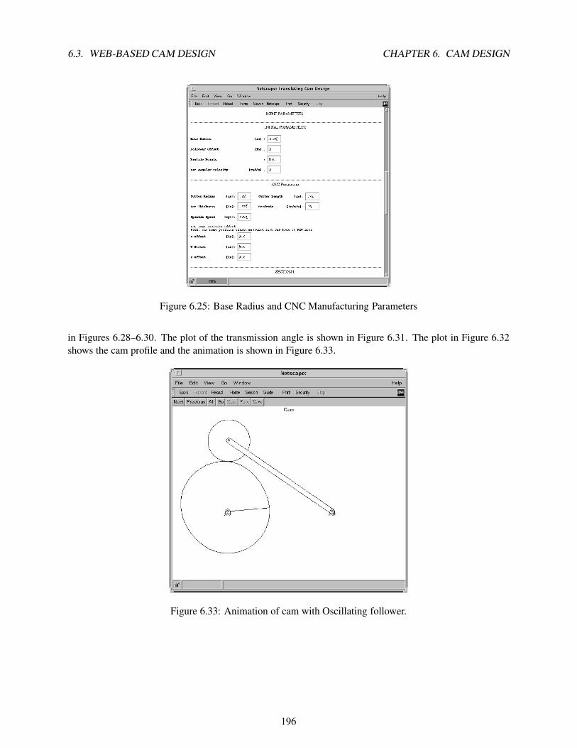
6.3. WEB-BASED CAM DESIGN CHAPTER 6. CAM DESIGN
Figure 6.25: Base Radius and CNC Manufacturing Parameters
in Figures 6.28–6.30. The plot of the transmission angle is shown in Figure 6.31. The plot in Figure 6.32
shows the cam profile and the animation is shown in Figure 6.33.
Figure 6.33: Animation of cam with Oscillating follower.
196

6.3. WEB-BASED CAM DESIGN CHAPTER 6. CAM DESIGN
Figure 6.26: Section Parameters
Figure 6.27: Translating cam output options
197

6.3. WEB-BASED CAM DESIGN CHAPTER 6. CAM DESIGN
Figure 6.28: Oscillating follower position.
Figure 6.29: Oscillating follower velocity.
198

6.3. WEB-BASED CAM DESIGN CHAPTER 6. CAM DESIGN
Figure 6.30: Oscillating follower acceleration.
Figure 6.31: Transmission angle of the cam.
199

6.3. WEB-BASED CAM DESIGN CHAPTER 6. CAM DESIGN
Figure 6.32: Cam profile.
200

Chapter 7
Quick Animation
Figure 7.1: Quick Animation window showing a four-bar linkage
All animations of Ch Mechanism Toolkit are handled by QuickAnimationTM. QuickAnimationTM
can display and animate various planar mechanical systems based on specified x-y coordinate data. For
example, the QuickAnimationTM window shown in Figure 7.1 displays a menu bar and a four-bar mecha-
nism. The mechanism is drawn in the largest area of the window with the name of the mechanism above it.
Links are drawn as lines, joints are drawn as open circles, and coupler points are drawn as filled circles. The
triangular area represents one solid link to which a coupler point is attached. The coupler curve is drawn
to indicate the motion of the coupler point. The details on how to use the QuickAnimationTM program of
qanimate for animation of planar mechanisms are described in this chapter.
201

7.1. THE USER INTERFACE FOR QUICKANIMATIONTM CHAPTER 7. QUICK ANIMATION
7.1 The User Interface for QuickAnimationTM
The menu bar in the Quick Animation window, as shown in Fig. 7.1, contains two menus, File and
Options, and a series of buttons which manipulate the mechanism. The File menu allows one to quit
the program and the Options menu allows one to change various display settings. The Next and Prev
buttons control the mechanism’s position, and the All button displays all mechanism positions at once. The
Fast and Slow buttons change the speed of animation. The Go and Stop buttons start and stop animation,
respectively. The mechanism can move in either direction by pressing the Prev button for one direction
and the Next button for the opposite direction. When the Go button is pressed, the mechanism will move
in the direction previously assigned by the Prev or Next button.
7.2 Input Data Format
The typical format for a Quick Animation data file is displayed in Figure 7.2. It is specified with the
following typographical notation:
• Typewriter text specifies actual keywords.
• Emphasized text is specified by the user.
• Text between square brackets ‘[]’ are optional.
• The line character ‘|’ specifes an “OR” condition.
The character ‘#’ on the first line delimits a comment. QuickAnimation will ignore anything on that line
following the ‘#’ character. The title of the mechanical system is specified by the title keyword fol-
lowed by the title string delimited by the double quotation character, ‘"’. Keyword fixture allows the
following lines to define the fixed objects. The primitives are commands used to define general and
mechanical components of the displayed or animated system. The animate begins the inputting of of data
for animation. Each line following keyword animate represents one frame of the animation, as indicated
by the superscript on primitive. The option restart specifies that when the animation is finished, it
starts again from the beginning. The option reverse specifies that when the animation is finished, it starts
the animatin backwards from the last frame till the first frame. The primitives following the keyword
stopped will be displayed only when animation is stopped. A frame consists of a data set that can con-
tain multiple primitives. The continuation character ’\’ can be used to span premitives in a data set over
multiple lines. An animation with n number of frames requres n number of data sets.
7.2.1 General Drawing Primitives
Figure 7.3 shows the various drawing primitives available for Quick Animation. These primitives allow
for the drawing of an arc, line, segment, circle, polygon, and rectangle as well as the insertion of text into
a Quick Animation program. The syntax for drawing such primitives are displayed in Figure 7.4. As an
example, consider the sytax for drawing a line. One may specify a line by typing line followed by the
x- and y-coordinates of the starting and ending points of the line (i.e. line 0 0 2 3 draws a line from
the origin to point (2,3) in the Cartesian coordinate system). Multiple lines may be linked together by
adding more coordinate points after the line statement. Similarly, a circle may be drawn by specifying
its center point and radius according to the syntax in Figure 7.4. The various options available for each
general drawing primitives are displayed in Figure 7.5, and an example of color and font options is listed in
Figure 7.6.
202

7.2. INPUT DATA FORMAT CHAPTER 7. QUICK ANIMATION
# comment
title "title string"
fixture
primitives
animate [ restart | reverse ]
primitives1 [ stopped primitives1 ]
primitives2 [ stopped primitives2 ]
.
.
.
primitivesn [ stopped primitivesn ]
Figure 7.2: Quick Animation data format.
2(x , y )
2
Segment
1(x , y )
1
nn(x , y )
2(x , y )
2
Line
(x, y) string
Text
(x, y)radius
Circle
Polygon
(x, y)
(x, y)
height
angle
width
1(x , y )
1
2(x , y )
2
nn(x , y )
1(x , y )
1
Arc
width
angle1
angle2
height
Rectangle
Figure 7.3: Graphical representation of general drawing primitives
203

7.2. INPUT DATA FORMAT CHAPTER 7. QUICK ANIMATION
line x1 y1 x2 y2 [ . . . xn yn ]arc x y width height angle1 angle2
segment x1 y1 x2 y2rectangle x y width height [ angle angle ]
polygon x1 y1 x2 y2 x3 y3 . . . xn yntext x y string
circle x y radius
dot x y
Figure 7.4: Syntax for general drawing primitives
line
segment . . .[ pen color ]
[ linewidth pixelwidth ]
[ linestyle solid |
dashed [ length pixellength ] |
dotted [ gap pixelgap ] ]
[ capstyle butt | round | projecting ]
[ joinstyle miter | round | bevel ]
[ depth depth ]
arc
circle
polygon
rectangle . . .[ pen color ]
[ fill color [ intensity percent ]
[ pattern number ] ]
[ linewidth pixelwidth ]
[ linestyle solid |
dashed [ length pixellength ] |
dotted [ gap pixelgap ] ]
[ capstyle butt | round | projecting ]
[ joinstyle miter | round | bevel ]
[ depth depth ]
text . . .[ pen color ]
[ depth depth ]
[ font fontname ]
dot . . .[ pen color ]
[ depth depth ]
Figure 7.5: Options for general drawing primitives
204
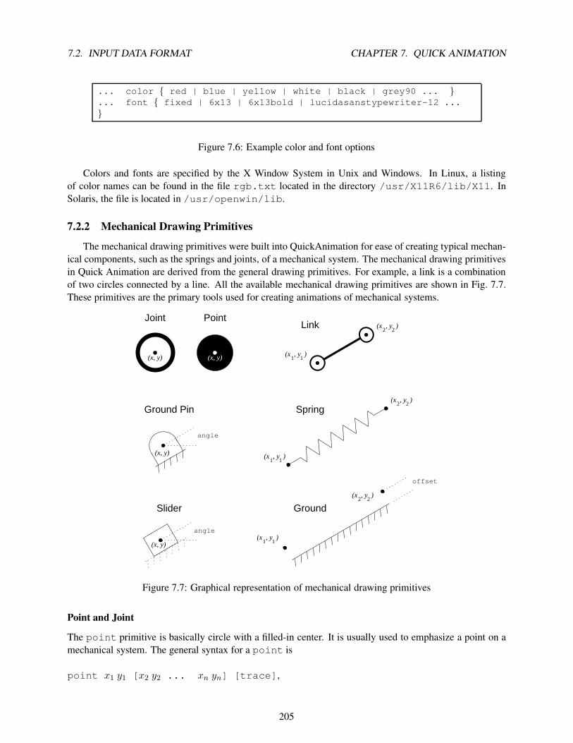
7.2. INPUT DATA FORMAT CHAPTER 7. QUICK ANIMATION
... color { red | blue | yellow | white | black | grey90 ... }
... font { fixed | 6x13 | 6x13bold | lucidasanstypewriter-12 ...
}
Figure 7.6: Example color and font options
Colors and fonts are specified by the X Window System in Unix and Windows. In Linux, a listing
of color names can be found in the file rgb.txt located in the directory /usr/X11R6/lib/X11. In
Solaris, the file is located in /usr/openwin/lib.
7.2.2 Mechanical Drawing Primitives
The mechanical drawing primitives were built into QuickAnimation for ease of creating typical mechan-
ical components, such as the springs and joints, of a mechanical system. The mechanical drawing primitives
in Quick Animation are derived from the general drawing primitives. For example, a link is a combination
of two circles connected by a line. All the available mechanical drawing primitives are shown in Fig. 7.7.
These primitives are the primary tools used for creating animations of mechanical systems.
offset
2(x , y )
2
1(x , y )
1
2(x , y )
2
1(x , y )
1
1
Slider
(x, y)
Point
2
angle
(x, y)
angle
(x, y)
(x , y )2
1(x , y )
Spring
LinkJoint
(x, y)
Ground Pin
Ground
Figure 7.7: Graphical representation of mechanical drawing primitives
Point and Joint
The point primitive is basically circle with a filled-in center. It is usually used to emphasize a point on a
mechanical system. The general syntax for a point is
point x1 y1 [x2 y2 ... xn yn] [trace],
205
7.2. INPUT DATA FORMAT CHAPTER 7. QUICK ANIMATION
where x1y1...xnyn specify the coordinate(s) of the joint(s), trace is an optional parameter used to specify
whether the point is to be traced during animation. For example, to create a point at coordinate (1,3) with a
trace the following command would be required:
point 1 3 trace.
Primitive joint is very similar to point. It is syntatically the same as the point primitive, but
is comprised of a circle that is not filled-in. The joint represents a connection between two links or other
mechanical components.
Link
As previously mentioned, the link primitive is a mechanical component formed by two circle primitives
and a line primitive. This primitive is normally used for generating animations of mechanical linkages such
as fourbar mechanisms. The general syntax for a link is given by the following:
link x1 x2 x2 y2 [... xn yn].
The coordinates of the endpoints of the first link is specified by (x1,y1) and (x2,y2). Addition links may
be attached to the last link by indicating the coordinates of the links’ other endpoints. A typical example of
creating two links adjoined at a common endpoint would be
link 1 1 1 4 4 4
In this example, the endpoints of the first link are at coordinates (1,1) and (1,4). The second link is then
attached to the first link at (1,4), and its other endpoint is located at (4,4). Note that the extra space between
the endpoint coordinates are ignored during execution of the Quick Animation program. They are present
in the example to help distinguish the endpoints.
Ground
The ground primitive represents a reference area of the animation. It is stationary and fixed to its location.
The syntax for ground is
ground x1 y1 x2 y2 [offset pixeloffset]
[ticks forward | backward]
For option offset, pixeloffset specifies the distance that the ground should be placed away for the x-
and y-coordinates of the ground. Additionally, if the ticks option is used, and its value is ”forward”, then
the ground is specified as going from (x1,y1) to (x2,y2). Likewise, the opposite is true if the value of ticks
is ”backward”. The default value for option ticks is ”forward”. For example,
ground 0 0 10 0 offset 2
will produce a ”ground” section from x=0 to x=10 and two units below the line, y=0.
Ground Pin
In order to directly connect a mechanical system to ”ground”, the groundpin primitive is used to specify
the desired connection. The syntax for this primitive is given below as
206

7.3. QUICK ANIMATION EXAMPLES CHAPTER 7. QUICK ANIMATION
groundpin x y [angle angle]
Coordinate (x,y) is the center point of the ground pin, and the optional argument angle angle describes
the angular offset, in radians, relative to a horizontal position. In order to create a ground pin at the origin
with a 45◦ rotational offset, the following statement should be declared:
groundpin 0 0 angle 45
Slider
The slider primitive is generated from the rectangle drawing primitive. It represents a block member of
a mechanical system that is only capable of translation displacement. Similar to the ground pin, the slider
can have an angular displacement that would allow it to translate on a sloped surface. Its syntax is defined
as follow:
slider x y [angle angle]
As an example, consider a crank-slider mechanism that requires the slider to slide on a sloped surface,
located at (3,4) that is about 30◦ relative to the ground. The slider portion of the mechanism can be created
with the following statement:
slider 3 4 angle 30
Spring
The spring is a typical component of many mechanical systems. The availability of a spring primitive in
Quick Animation greatly increases the number of mechanical systems that can be modeled and animated.
Its syntax is given as
spring x1 y1 x2 y2,
where coordinates (x1,y1) and (x2,y2) specifies the endpoints of the spring. To create a spring from (1,1) to
(3,5), the following should be entered in the Quick Animation data file:
spring 1 1 3 5
7.3 Quick Animation Examples
The data file in Figure 7.8 illusrates how general and mechanical primitives are specified in a quick animation
file. Figure 7.9 show the display when this data file is processed by the program.
The sample code shown in Figure 7.10 can be used to create an animation of a fourbar linkage similar
to the one in Figure 7.11. A comment line in an animation file starts with #qanimate. Next, the title
of the animation is set, and the fixtures are specified as ground pins at points (Ax, Ay) and (Dx,Dy).Line animate restart is used to begin the input of the animation. Each line beginning with (line
...) and ending after (polygon ...) represents one snap shot, or one position, of the fourbar linkage
animation. The links are drawn with the link keyword. Each coordinate pair represents a joint of the
mechanism. On each line, the coordinate pairs are arranged in order so that two adjacent joints form a link.
207

7.3. QUICK ANIMATION EXAMPLES CHAPTER 7. QUICK ANIMATION
# this is a comment
title "This is a Title"
fixture
#no fixture
animate
# low level primitives:
line 0 0 1 1.5 2 2 pen red \
line 3 3 4 4
line 5 5 12 5 linestyle dashed length 2 pen green linewidth 1
line 5 6 12 6 linestyle dashed length 5 pen green linewidth 1
line 5 7 12 7 linestyle dotted gap 1 pen red linewidth 2
line 5 8 12 8 linestyle dotted gap 5 pen red linewidth 2
arc 11 11 4 4 0 270 fill grey90 linewidth 5
arc 12 12 10 11 0 90 13 13 5 5 0 360 linewidth 2 pen blue
segment 14 14 15 15 16 16 17 17 pen red
#color of text cannot be changed in Windows for now
text 18 5 string1 pen rgb:ffff/ffff/0
text 18 7 "This is a string2" pen red
text 18 9 "This is a string3" \
font -*-lucidatypewriter-medium-*-*-*-12-*-*-*-*-*-*-*circle 22 16 2 \
stopped line 14 17 17 20 text 17.2 20 "center of circle"
rectangle 15 18 1 1 pen red fill grey
rectangle 17 20 2 1 angle 30
# higher linkage primitives
joint 18 18
point 19 19
link 20 20 21 21
groundpin 22 22 25 25 angle 30
link 22 22 25 25
polygon 4 10 5 10 6 13 3.5 14 fill green
spring 10 1 15 1
ground 17 1.0 19 2.0
# The traced trajectory shown on the upper left
point 0 20 trace
point 3 23 trace
point 6 25 trace
point 10 20 trace
Figure 7.8: A sample data file sample.1nm.
208

7.3. QUICK ANIMATION EXAMPLES CHAPTER 7. QUICK ANIMATION
Figure 7.9: The quick animation display based on the sample data file sample.qnm.
209

7.3. QUICK ANIMATION EXAMPLES CHAPTER 7. QUICK ANIMATION
#qanimate animation file
title "Crank-Rocker"
fixture
groundpin Ax Ay Dx Dy
animate restart
link A1x A
1y B1
x B1y C1
x C1y D1
x D1y \
point trace P 1x P
1y \
polygon fill grey B1x B
1y C1
x C1y P 1
x P1y
link A2x A
2y B2
x B2y C2
x C2y D2
x D2y \
point trace P 2x P
2y \
polygon fill grey B2x B
2y C2
x C2y P 2
x P2y
.
.
.
link Anx A
ny Bn
x Bny Cn
x Cny Dn
x Dny \
point trace Pnx Pn
y \
polygon fill grey Bnx B
ny Cn
x Cny Pn
x Pny
Figure 7.10: Input data format for a four-bar linkage with a single coupler point
210

7.3. QUICK ANIMATION EXAMPLES CHAPTER 7. QUICK ANIMATION
The path of the coupler point, specified as point P in Figure 7.11, is shown with a point trace. The
polygon keyword was used to create the coupler attachment.
Figure 7.11: General fourbar linkage
Before viewing a complete Ch program for creating a Quick Animation data file, consider the Ch code
listed as Figure 7.12. This Ch code can be executed to create one frame of animation data. First, the
variables for the fourbar parameters are declared and initialized. Then printf() statements are used to write
the typical heading of an animation data file. Note that the links and coupler point vector are represented
as complex variables R and P, where R is an array of complex type. The positions of the links and coupler
point are calculated by the complexsolveRR() function and vector analysis. Additional calls to function
printf() completes writing to the animation data file. The resulting animation code of the program shown in
Figure 7.12 can be used by the Quick Animation application to generate a single frame of animation, which
is shown as Figure 7.13.
211

7.3. QUICK ANIMATION EXAMPLES CHAPTER 7. QUICK ANIMATION
/* Filename: fourbar_pos.ch */
#include <stdio.h>
#include <math.h>
#include <complex.h>
#define deg2rad(a) ((a)*M_PI/180.0) // macros
#define rad2deg(a) ((a)*180.0/M_PI)
int main() {
double theta1 = deg2rad(20.0), // given data
r1 = 5.5,
r2 = 1.5,
r3 = 4.5,
r4 = 5,
rp = 3,
beta = deg2rad(25.0);
double theta2,theta3,theta4, theta3_2, theta4_2;
double complex z;
double complex R[1:3]; // link vectors
double complex P; // coupler vector
R[1] = polar(r1,theta1);
/* The comment */
printf("#qanimate animation data\n");
/* The title displayed on the animation */
printf("title Crank-Rocker\n");
printf("fixture\n");
/* The primitives following fixture */
printf("groundpin 0 0 %g %g\n", real(R[1]), imag(R[1]));
/* For crank-rocker, crank-crank, use animate restart.
For rocker-rocker, rocker-crank, use animate reverse */
printf("animate restart\n");
theta2 = deg2rad(10.0);
z = polar(r1,theta1) - polar(r2,theta2);
complexsolveRR(r3,-r4,z,theta3, theta4, theta3_2, theta4_2);
R[2] = polar(r2,theta2);
R[3] = R[2] + polar(r3,theta3);
P = R[2] + polar(rp,theta3+beta);
/* output coordinates for animation */
printf("link 0 0 %f %f %f %f %f %f \\\n",
real(R[2]), imag(R[2]),
real(R[3]), imag(R[3]),
real(R[1]), imag(R[1]) );
printf("point trace %f %f \\\n", real(P), imag(P));
printf("polygon fill grey90 %f %f %f %f %f %f \\\n",
real(R[2]), imag(R[2]),
real(R[3]), imag(R[3]),
real(P), imag(P));
printf("\n");
}
Figure 7.12: List of program fourbar pos.ch.
212

7.3. QUICK ANIMATION EXAMPLES CHAPTER 7. QUICK ANIMATION
Figure 7.13: Single animation frame of a fourbar linkage.
Figure 7.14 lists a sample Ch code used to create a Quick Animation data file. The animation can be
created by typing the following in the Ch command prompt:
fourbar_pos.ch | qanimate
or
fourbar_pos.ch > tmp1.qnm
qanimate tmp1.qnm
The result of fourbar pos.ch is shown in Figure 7.15. The data sets for creating the fourbar linkage
animation is typically generated by a for loop in Ch code. Figure 7.16 displays a snapshot of the Quick
Animation animation generated by the animation data file.
213

7.3. QUICK ANIMATION EXAMPLES CHAPTER 7. QUICK ANIMATION
/**********************************************************************
* fourbar_ani1.ch
*
* Purpose:
* - fourbar linkage analysis
* - output animation coordinate data
* Run this program in CH as follows:
* in Unix:
* fourbar_ani1.ch | qanimate
* or
* fourbar_ani1.ch > tmp1.qnm
* qanimate tmp1.qnm
* in Windows:
* fourbar_ani1.ch | qanimate
* or
* fourbar_ani1.ch > tmp1.qnm
* qanimate tmp1.qnm
* or
* fourbar_ani1.ch > tmp1.qnm
* tmp1.qnm
**********************************************************************/
#include <stdio.h>
#include <math.h>
#include <complex.h>
#define deg2rad(a) ((a)*M_PI/180.0) // macros
#define rad2deg(a) ((a)*180.0/M_PI)
int main() {
double theta1 = deg2rad(20.0), // given data
r1 = 5.5,
r2 = 1.5,
r3 = 4.5,
r4 = 5,
rp = 3,
beta = deg2rad(25.0);
double theta2,theta3,theta4, theta3_2, theta4_2;
double complex z;
double complex R[1:3]; // link vectors
double complex P; // coupler vector
R[1] = polar(r1,theta1);
/* The comment */
printf("#qanimate animation data\n");
/* The title displayed on the animation */
printf("title Crank-Rocker\n");
printf("fixture\n");
/* The primitives following fixture */
printf("groundpin 0 0 %g %g\n", real(R[1]), imag(R[1]));
/* For crank-rocker, crank-crank, use animate restart.
For rocker-rocker, rocker-crank, use animate reverse */
printf("animate restart\n");
for (theta2=0.0; theta2<=deg2rad(360.0); theta2+=deg2rad(10.0)) {
z = polar(r1,theta1) - polar(r2,theta2);
complexsolveRR(r3,-r4,z,theta3, theta4, theta3_2, theta4_2);
R[2] = polar(r2,theta2);
R[3] = R[2] + polar(r3,theta3);
P = R[2] + polar(rp,theta3+beta);
/* output coordinates for animation */
printf("link 0 0 %f %f %f %f %f %f \\\n",
real(R[2]), imag(R[2]),
real(R[3]), imag(R[3]),
real(R[1]), imag(R[1]) );
printf("point trace %f %f \\\n", real(P), imag(P));
printf("polygon fill grey90 %f %f %f %f %f %f \\\n",
real(R[2]), imag(R[2]),
real(R[3]), imag(R[3]),
real(P), imag(P));
printf("\n");
}
}
214
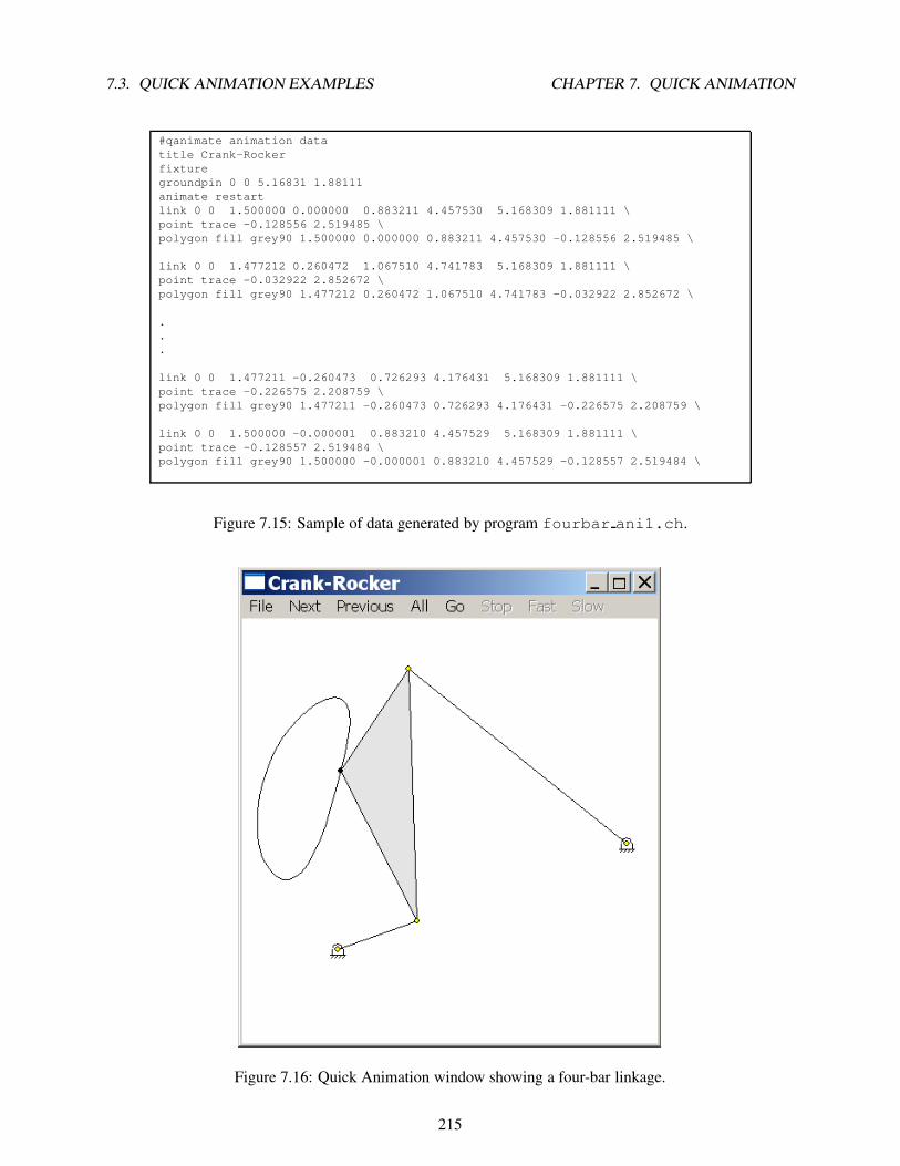
7.3. QUICK ANIMATION EXAMPLES CHAPTER 7. QUICK ANIMATION
#qanimate animation data
title Crank-Rocker
fixture
groundpin 0 0 5.16831 1.88111
animate restart
link 0 0 1.500000 0.000000 0.883211 4.457530 5.168309 1.881111 \
point trace -0.128556 2.519485 \
polygon fill grey90 1.500000 0.000000 0.883211 4.457530 -0.128556 2.519485 \
link 0 0 1.477212 0.260472 1.067510 4.741783 5.168309 1.881111 \
point trace -0.032922 2.852672 \
polygon fill grey90 1.477212 0.260472 1.067510 4.741783 -0.032922 2.852672 \
.
.
.
link 0 0 1.477211 -0.260473 0.726293 4.176431 5.168309 1.881111 \
point trace -0.226575 2.208759 \
polygon fill grey90 1.477211 -0.260473 0.726293 4.176431 -0.226575 2.208759 \
link 0 0 1.500000 -0.000001 0.883210 4.457529 5.168309 1.881111 \
point trace -0.128557 2.519484 \
polygon fill grey90 1.500000 -0.000001 0.883210 4.457529 -0.128557 2.519484 \
Figure 7.15: Sample of data generated by program fourbar ani1.ch.
Figure 7.16: Quick Animation window showing a four-bar linkage.
215

7.3. QUICK ANIMATION EXAMPLES CHAPTER 7. QUICK ANIMATION
Two additional examples of creating Quick Animation animation files are given below. They generate
the same fourbar linkage animation as that of program fourbar ani1.ch, but with special handling of
the animation data. Program fourbar ani2.ch outputs the animation coordinate data to two data files
fourbar ani1.qnm and fourbar ani2.qnm, one file for each kinematic inversion of the fourbar
linkage. These animation data files are then processed by program qanimate. Program fourbar ani3.ch
will also produce two data files, but these data files are piped directly to the Quick Animation program to
automatically generate the fourbar linkage animations. No extra commands are required to implement an-
imation for the third sample program. Execution of the program will simply generate the desired animations.
Listing of program fourba ani2.ch
/**********************************************************************
* fourbar_ani2.ch
* Purpose:
* - fourbar linkage analysis
* - output animation coordinate data to two data files and run animation
* Run this program in Ch as follows:
* fourbar_ani2.ch
**********************************************************************/
#include <stdio.h>
#include <math.h>
#include <complex.h>
#define deg2rad(a) ((a)*M_PI/180.0) // macros
#define rad2deg(a) ((a)*180.0/M_PI)
int main() {
double theta1 = deg2rad(20.0), // given data
r1 = 5.5,
r2 = 1.5,
r3 = 4.5,
r4 = 5,
rp = 3,
beta = deg2rad(25.0);
int i;
double theta2,theta3,theta4,theta3_2,theta4_2;
double complex z;
double complex R[1:3]; // link vectors
double complex P; // coupler vector
FILE *out[2];
R[1] = polar(r1,theta1);
out[0] = fopen("fourbar_ani1.qnm","w"); // open fourbar_ani1.qnm
if (!out[0]) {
perror("fopen()");
exit(1);
}
out[1] = fopen("fourbar_ani2.qnm","w"); // open fourbar_ani2.qnm
if (!out[1]) {
perror("fopen()");
exit(1);
}
for (i=0; i<2; i++) {
/* The first line of the animation file must start with #qanimate */
fprintf(out[i],"#qanimate animation data\n");
/* The title displayed on the animation */
216

7.3. QUICK ANIMATION EXAMPLES CHAPTER 7. QUICK ANIMATION
fprintf(out[i],"title Crank-Rocker\n");
fprintf(out[i],"fixture\n");
/* The primitives following fixture */
fprintf(out[i],"groundpin 0 0 %g %g\n", real(R[1]), imag(R[1]));
/* For crank-rocker, crank-crank, use animate restart.
For rocker-rocker, rocker-crank, use animate reverse */
fprintf(out[i],"animate restart\n");
}
for (theta2=0.0; theta2<=deg2rad(360.0); theta2+=deg2rad(10.0)) {
R[2] = polar(r2,theta2);
z = polar(r1,theta1) - polar(r2,theta2);
complexsolveRR(r3,-r4,z,theta3,theta4, theta3_2, theta4_2);
/* first solution */
R[3] = R[2] + polar(r3,theta3);
P = R[2] + polar(rp,theta3+beta);
/* output coordinates for animation */
fprintf(out[0],"link 0 0 %f %f %f %f %f %f \\\n",
real(R[2]), imag(R[2]),
real(R[3]), imag(R[3]),
real(R[1]), imag(R[1]) );
fprintf(out[0],"point trace %f %f \\\n", real(P), imag(P));
fprintf(out[0],"polygon fill grey90 %f %f %f %f %f %f \\\n",
real(R[2]), imag(R[2]),
real(R[3]), imag(R[3]),
real(P), imag(P));
fprintf(out[0],"\n");
/* second solution */
R[3] = R[2] + polar(r3,theta3_2);
P = R[2] + polar(rp,theta3_2+beta);
/* output coordinates for animation */
fprintf(out[1],"link 0 0 %f %f %f %f %f %f \\\n",
real(R[2]), imag(R[2]),
real(R[3]), imag(R[3]),
real(R[1]), imag(R[1]) );
fprintf(out[1],"point trace %f %f \\\n", real(P), imag(P));
fprintf(out[1],"polygon fill grey90 %f %f %f %f %f %f \\\n",
real(R[2]), imag(R[2]),
real(R[3]), imag(R[3]),
real(P), imag(P));
fprintf(out[1],"\n");
}
fclose(out[0]);
fclose(out[1]);
qanimate fourbar_ani1.qnm
remove("fourbar_ani1.qnm"); // remove the data file
qanimate fourbar_ani2.qnm
remove("fourbar_ani2.qnm"); // remove the data file
}
Listing of program fourbar ani3.ch
/**********************************************************************
217

7.3. QUICK ANIMATION EXAMPLES CHAPTER 7. QUICK ANIMATION
* fourbar_ani3.ch
*
* Purpose:
* - fourbar linkage analysis
* - output animation coordinate data to two pipes
* Run this program in Ch as follows:
* fourbar_ani3.ch
**********************************************************************/
#include <stdio.h>
#include <math.h>
#include <complex.h>
#define deg2rad(a) ((a)*M_PI/180.0) // macros
#define rad2deg(a) ((a)*180.0/M_PI)
int main() {
double theta1 = deg2rad(20.0), // given data
r1 = 5.5,
r2 = 1.5,
r3 = 4.5,
r4 = 5,
rp = 3,
beta = deg2rad(25.0);
int i;
double theta2,theta3,theta4,theta3_2,theta4_2;
double complex z;
double complex R[1:3]; // link vectors
double complex P; // coupler vector
FILE *out[2];
R[1] = polar(r1,theta1);
out[0] = popen("qanimate","w"); // open qanimate pipe
if (!out[0]) {
perror("popen()");
exit(1);
}
out[1] = popen("qanimate","w");
if (!out[1]) {
perror("popen()");
exit(1);
}
for (i=0; i<2; i++) {
/* The comment */
fprintf(out[i],"#qanimate animation data\n");
/* The title displayed on the animation */
fprintf(out[i],"title Crank-Rocker\n");
fprintf(out[i],"fixture\n");
/* The primitives following fixture */
fprintf(out[i],"groundpin 0 0 %f %f\n", real(R[1]), imag(R[1]));
/* For crank-rocker, crank-crank, use animate restart.
For rocker-rocker, rocker-crank, use animate reverse */
fprintf(out[i],"animate restart\n");
}
for (theta2=0.0; theta2<=deg2rad(360.0); theta2+=deg2rad(10.0)) {
R[2] = polar(r2,theta2);
z = polar(r1,theta1) - polar(r2,theta2);
218

7.3. QUICK ANIMATION EXAMPLES CHAPTER 7. QUICK ANIMATION
complexsolveRR(r3,-r4,z,theta3,theta4, theta3_2, theta4_2);
/* first solution */
R[3] = R[2] + polar(r3,theta3);
P = R[2] + polar(rp,theta3+beta);
/* output coordinates for animation */
fprintf(out[0],"link 0 0 %f %f %f %f %f %f \\\n",
real(R[2]), imag(R[2]),
real(R[3]), imag(R[3]),
real(R[1]), imag(R[1]) );
fprintf(out[0],"point trace %f %f \\\n", real(P), imag(P));
fprintf(out[0],"polygon fill grey90 %f %f %f %f %f %f \\\n",
real(R[2]), imag(R[2]),
real(R[3]), imag(R[3]),
real(P), imag(P));
fprintf(out[0],"\n");
/* second solution */
R[3] = R[2] + polar(r3,theta3_2);
P = R[2] + polar(rp,theta3_2+beta);
/* output coordinates for animation */
fprintf(out[1],"link 0 0 %f %f %f %f %f %f \\\n",
real(R[2]), imag(R[2]),
real(R[3]), imag(R[3]),
real(R[1]), imag(R[1]) );
fprintf(out[1],"point trace %f %f \\\n", real(P), imag(P));
fprintf(out[1],"polygon fill grey90 %f %f %f %f %f %f \\\n",
real(R[2]), imag(R[2]),
real(R[3]), imag(R[3]),
real(P), imag(P));
fprintf(out[1],"\n");
}
pclose(out[0]);
pclose(out[1]);
}
219

Chapter 8
Implementations of Interactive Web Pages
for Mechanism Design and Analysis
Interactive web-based mechanism analysis for various linkages have been introduced in the previous chap-
ters. From those brief introductions, it can be seen that web-based analysis was a convenient tool for per-
forming kinematic and dynamic analysis of the mechanisms. Users only have to input specific values for
the mechanism they want to study and then click on the ”run” button to begin the mechanism analysis. This
saves the user valuable time since the computer is performing all the required calculations, and he/she does
not need to have any prior programming experiences.
This chapter will provide a more in depth discussion on how the interactive mechanism analysis web
pages are designed and implemented. At the end of the chapter, the user should have a clear understanding
of the functionality of interactive web-based analysis programs and be able to develop similar web pages.
8.1 Introduction to CGI Programming
The basis behind the concept of interactive web-based mechanism analysis is CGI programming. CGI,
or Common Gateway Interface, allows web servers to execute scripts and programs using data sent by a
client and then returns the results to the client. The web pages for mechanism analysis utilizes Ch scripts to
perform the desired analysis. CGI programming involves the interaction between two files: an HTML file
and a script/program file.
8.1.1 Writing HTML Files
HTML files allows for the creation of internet web pages that web servers utilize to prompt users to input
data required by CGI scripts. For example, consider the ”fill-out form” web page shown in Figure 8.1. It is
a simple HTML document for sending data through a web page.
HTML is not a programming language, but a formatting language. Formatting is specified by tags in
HTML files. Tags can be easily distinguished from other text in HTML files because they are enclosed
within a pair of angle brackets, <...>. For example, <TITLE> and <BODY> are two HTML tags used in
Program 46. Furthermore, tags and other elements in HTML code are case insensitive. Thus, <TITLE> is
equivalent to <Title> or <Title>. Table 8.1 lists some of the common HTML tags along with a brief
description. Note that some format tags requires an ending statement, such as <BODY>...</BODY>.
All HTML documents should have a clearly defined head and body. The head of an HTML document
usually includes the title of the document. Note that the title does not appear inside the body of document,
but instead, displayed in the window’s title bar for the web browser. The head and title are delimited by
220
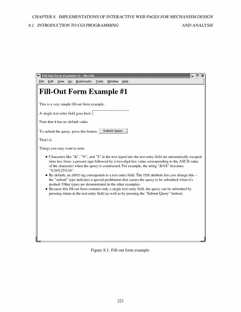
8.1. INTRODUCTION TO CGI PROGRAMMING
CHAPTER 8. IMPLEMENTATIONS OF INTERACTIVE WEB PAGES FOR MECHANISM DESIGN
AND ANALYSIS
Figure 8.1: Fill-out form example.
221

8.1. INTRODUCTION TO CGI PROGRAMMING
CHAPTER 8. IMPLEMENTATIONS OF INTERACTIVE WEB PAGES FOR MECHANISM DESIGN
AND ANALYSIS
<HEAD>
<TITLE>Fill-Out Form Example #1</TITLE>
</HEAD>
<BODY bgcolor="#FFFFFF" text="#000000" vlink="#FF0000">
<H1>Fill-Out Form Example #1</H1>
This is a very simple fill-out form example. <P>
<FORM METHOD="POST" ACTION="/cgi-bin/chcgi/form.ch">
A single text entry field goes here: <INPUT NAME="entry"> <P>
Note that it has no default value. <P>
To submit the query, press this button: <INPUT TYPE="submit"
VALUE="Submit Query">. <P>
</FORM>
That’s it. <P>
Things you may want to note: <P>
<UL>
<LI> Characters like "&", "%", and "$" in the text typed into the
text entry field are automatically escaped (into hex form: a
percent sign followed by a two-digit hex value corresponding to
the ASCII value of the character) when the query is constructed.
For example, the string "&%$" becomes "%26%25%24".
<LI> By default, an <CODE>INPUT</CODE> tag corresponds to a text entry
field. The <CODE>TYPE</CODE> attribute lets you change this --
the "submit" type indicates a special pushbutton that causes the
query to be submitted when it’s pushed. Other types are
demonstrated in the other examples.
<LI> Because this fill-out form contains only a single text entry
field, the query can be submitted by pressing return in the text
entry field (as well as by pressing the "Submit Query" button).
</UL>
</BODY>
Program 46: HTML source code for Figure 8.1.
222

8.1. INTRODUCTION TO CGI PROGRAMMING
CHAPTER 8. IMPLEMENTATIONS OF INTERACTIVE WEB PAGES FOR MECHANISM DESIGN
AND ANALYSIS
<HEAD>...</HEAD> and <TITLE>...</TITLE>, respectively. For example, the title of the HTML
document shown in Figure 8.1 is ”Fill-Out Form Example #1”.
The source code for the HTML document of Figure 8.1 is Program 46. As can be seen from this source
code, the body of an HTML document contains all the information displayed on the internet web page.
Notice that some attributes have been specified for the HTML document within the <BODY> tag. The
bgcolor= attribute sets the background color of the web page, whereas attribute text= defines the color
of the text to be displayed. The last attribute, vlink=, specifies the color of a previously visited hyperlink.
In order to have a visible title displayed on the web page, the header tag <H1>...</H1> has been used.
Creating a form begins with the <FORM> tag. Within the <FORM> tag, there is typically two attributes
associated with it: method= and action=. For the example of Program 46, the form method is set to
post, which means that the data are to be passed via the standard input method. The action= attribute is
used to indicate the program or script to process the data collected by the HTML form. Inside the form, data
entry fields are specified with the <INPUT> tag. Note that data entry fields may be distinguished by names
with the name= attribute, as in Program 46. Submission of data is accomplished through the <INPUT> tag
with type= attribute set to ”submit”.
Table 8.1: Description of HTML tags.
Tags Description
<TITLE>...</TITLE> Specify title of an HTML document.
<HEAD>...</HEAD> Indicates the head section of an HTML document.
<BODY>...</BODY> Indicates the body section of an HTML document.
<H[#]>...</H[#]> Heading format; value of [#] can range from 1 to 6,
with <H1> being the highest setting.
<HR> Horizontal rule; inserts a horizontal line between
sections of text.
<CENTER>...</CENTER> Horizontal centering.
<IMG> Insert an in-line image.
<PRE>...</PRE> Display text in preformatted form.
<P> Paragraph tag; inserts a blank line between sections
of text.
<UL>...<LI>...</UL> Unordered, or unnumbered, list.
<BR> Break tag; starts new line, but does not insert a blank
one.
<B>...</B> Bold text.
<I>...</I> Italics text.
<U>...</U> Underline text.
<FORM>...</FORM> Define a form field within an HTML document.
<INPUT> Define an input field.
<SELECT>...</SELECT> Define a selection field.
8.1.2 Writing CGI Script Files
Processing data sent from an HTML document with the <FORM> tag requires a script file, which is located
on the server side. Once data are passed to the server through CGI, the necessary procedures are performed
and the result is returned to the client. As an example, Program 47 is the Ch script associated with the
223

8.1. INTRODUCTION TO CGI PROGRAMMING
CHAPTER 8. IMPLEMENTATIONS OF INTERACTIVE WEB PAGES FOR MECHANISM DESIGN
AND ANALYSIS
#!/bin/ch
#include <cgi.h>
int main() {
int i, num;
chstrarray name, value;
class CResponse Response;
class CRequest Request;
Response.begin();
Response.title("CGI FORM results");
printf("<H1>CGI FORM test script reports:</H1>\n");
num = Request.getFormNameValue(name, value);
if(num == 0) {
printf("No name/value has been submitted<P>\n");
exit(0);
}
else if(num < 0) {
printf("Error: in Request.getFormNameValue() <P>\n");
exit(0);
}
printf("The following %d name/value pairs are submitted<P>\n",num);
printf("<UL>\n");
for(i=0; i < num; i++) {
printf("<LI> <CODE>%s = ",name[i]);
if(value[i])
printf("%s",value[i]);
printf("</CODE>\n");
}
printf("</UL>\n");
Response.end();
}
Program 47: Example CGI program.
form filling example in the above section. It is used to process the data collected from the HTML document
shown in Figure 8.1, which is generated by Program 46.
The first line of Program 47, #!/bin/ch, indicates that this program is a Ch script file. Header file
cgi.h contains the definitions for classes CResponse and CRequest, which are convenient for CGI pro-
gramming. Class CRequest can be used to obtain data from HTML documents, whereas class CResponse
can be used to output data as an HTML document. Two generic data types chchar and chstrarray are also
type-defined in this header file. They are type-defined as follows.
typedef char chchar;
typedef char** chstrarray;
Program 47 declares two variables, name and value, of data type chstrarray to store the name and
value data passed by the form of Program 46. Member function begin() of class CResponse indicates the
start of the output. The title of the dynamically generated HTML document may be added with member
function title(), which requires a string for its input argument. For the document generated by Program 47,
the title is specified as "CGI FORM results". Lines of HTML codes are added with the C printf()
function. The names and values submitted in a fill-out form can be obtained by the CGI program by member
functions CResquest::getForm(), CResquest::getForms(), or CResquest::getFormNameValue(). For
224

8.2. WEB-BASED ANIMATION EXAMPLE
CHAPTER 8. IMPLEMENTATIONS OF INTERACTIVE WEB PAGES FOR MECHANISM DESIGN
AND ANALYSIS
Figure 8.2: Output of submitting form of Figure 8.1.
the example of Program 47, member function getFormNameValue() is used. The prototype for member
function getFormNameValue() is shown below.
int CRequest::getFormNameValue(chstrarray &names,
chstrarray &values);
The getFormNameValue() member function obtains all the name/value pairs from the HTML form doc-
ument and stores them into arguments names and values, which are treated as string arrays. After
obtaining the name/value pair(s) from the form-filling document, the rest of the code is used for checking
input errors and displaying the values that have been entered. Note that the primary function of HTML tag
<CODE> is to display codes extracted from programming files. Text are displayed as they are typed within
the tag. Figure 8.2 shows the dynamically generated HTML document after submitting the form shown in
Figure 8.1 with the entered value ”something”.
8.2 Web-Based Animation Example
Although the form-filling example in the above section provides a good introduction to CGI programming,
an in depth example is given in this section to show how to write a more effective CGI program. One such
example would be the fourbar animation web page discussed in Section 2.9. The HTML document for
animating the fourbar linkage mechanism via the internet is shown in Figure 2.20. Its source code is listed
as Program 48.
Program 48 concisely specifies the layout of Figure 2.20. After the head and title of the HTML doc-
ument, a figure of the fourbar linkage is displayed with the <IMG> tag, where option src= indicates the
location of the image file on the web server. Next, the <FORM> tag allows for the user to input data required
for generating the fourbar animation. The initial <SELECT> tag allow users to specify the use of SI of
US Customary units. Text input areas are created for link lengths and ground angle θ1. Furthermore, input
areas have been allocated for the coupler point properties if the user decides to specify a coupler link. Note
that each <INPUT> tag is associated with a name describing the required parameter. This allows the CGI
script, fourbar ani.ch, to easily identify the type of data being passed into it. For example, the CGI
script would be able to distinguish between link lengths r1 and r2. Along with the name= option for tag
<INPUT>, the options value= and size= specifies the default values and the field-width for each input,
respectively. Thus, the input for link length r4 has a default value of "5.0" and field width size of 5.
225

8.2. WEB-BASED ANIMATION EXAMPLE
Following the link lengths area, ground angle θ1 and the phase angle for the coupler point β may be
specified. The <SELECT> tag allows the user to specify whether the angles are in degrees or radians. The
branch number selection of the fourbar linkage is also created in this manner.
The CGI script for processing the data collected from the HTML form created by Program 48 is listed
as Program 49. Program 49 consists of the main() function and two other functions, errorHandler()
and fourbar ani(). In the main() function, an object of class CRequest, Request, is instantiated in
order to obtain the data submitted by the HTML form for animation of the fourbar mechanism. Member
function Request::getForm() is used to acquire the submitted data one value at a time. Member function
getForm() takes the name associated with the value to be acquired as an input value, and then the acquired
value becomes the member function’s return value. Note that the data values are read and stored as strings.
If, for some reason, the value submitted from the HTML form is invalid, function errorHandler() is
called to display an error message in HTML document form by using class CResponse.
If the values collected from the HTML form are all valid, then they are passed into function
fourbar ani() to simulate the motion of the fourbar linkage via the world wide web. In function
fourbar ani(), the data values passed in as strings are now converted to double precision floating-
point numbers, with the exceptions of arguments mode and branchnum. These two variables can be used
directly as strings. If the values for θ1 and β were submitted in degrees, then they are converted to radians
in function fourbar ani(). The next step to simulate the motion of the fourbar mechanism is to set the
parameters of object fourbar of class CFourbar. Once this is done, and the branch number of the fourbar
is determined from string branchnum, class CResponse can be used to stream the linkage animation to an
HTML document. Note that only a Rocker-Rocker mechanism may have a branch number greater than 2.
The statement
Response.setContentType("application/x-qnm");
indicates that the output is a Quick Animation application. Recall that member function
CFourbar:::animation() has a variable argument list. Also recall that if the second argument of member
function animation() is QANIMATE OUTPUTTYPE FILE, then the data for generating the fourbar ani-
mation can be saved into a file whose name is specified by a third function argument. For Program 49, the
second argument of member function animation() is QANIMATE OUTPUTTYPE STREAM, which indicates
that the animation data should be streamed directly to the HTML document.
An alternative CGI program for animating the fourbar linkage is Program 50. It is similar to Program 49,
except that this CGI program independently generates the animation data rather than use member function
CFourbar::animation(). However, Program 50 still incorporates the use of class CFourbar in order to
determine the joint limits and type of the fourbar. Vectors of double complex types are used to define the
various positions of the links and coupler point. In order to stream the animation to the web browser file
pointer animation is set to point to stdout. Program 50 is provided to show the reader how to create and
display animations on the internet with Quick Animation and CGI programming.
8.2.1 Configuration and Setup of Web Servers
In order to run the Quick Animation application from a Netscape Web server in a Unix operating system,
the following line has to be added to the Netscape WWW server configuration file mime.types located in
directory server home dir/https-80 or http/config.
type=application/x-qnm exts=qnm
For the Apache Web server, the line
226

8.2. WEB-BASED ANIMATION EXAMPLE
<HEAD>
<TITLE>
Interactive Four-Bar Linkage Animation
</TITLE>
</HEAD>
<BODY bgcolor="#FFFFFF">
<H1>
Interactive Four-Bar Linkage Animation
</H1>
<HR>
The four-bar linkage below can be animated on your screen.
<CENTER>
<IMG SRC="/chhtml/toolkit/mechanism/fig/fourbar/fourbar_trans.gif">
</CENTER>
<P>
<HR>
<FORM method="POST" action="/cgi-bin/chcgi/toolkit/mechanism/fourbar/fourbar_ani.ch">
<BR>
Unit Type:
<SELECT name="unit">
<OPTION value="SI">SI
<OPTION value="USC">US Customary
</SELECT>
<BR>
Link lengths (m or ft):
<B>r1:</B> <INPUT name="r1" value="0.12" size=5>
<B>r2:</B> <INPUT name="r2" value="0.04" size=5>
<B>r3:</B> <INPUT name="r3" value="0.10" size=5>
<B>r4:</B> <INPUT name="r4" value="0.07" size=5>
<B>rp:</B> <INPUT name="rp" value="0.05" size=5>
<BR>
Angles:
<B>theta1:</B> <INPUT name="th" value="0" size=6>
<B>beta:</B> <INPUT name="beta" value="20" size=6>
<SELECT name="mode">
<OPTION value="deg">Degree Mode
<OPTION value="rad">Radian Mode
</SELECT>
<BR>
Number of points: <INPUT name="n" value="30" size=3>
<BR><BR>
Program 48: Source code for web-based fourbar linkage animation.
227

8.2. WEB-BASED ANIMATION EXAMPLE
Branch Number:
<SELECT name="branchnum">
<OPTION value="1st">1
<OPTION value="2nd">2
<OPTION value="3rd">3
<OPTION value="4th">4
</SELECT>
<BR>
<P>
<INPUT TYPE=submit VALUE="Run">
<INPUT TYPE=reset VALUE="Reset">
</FORM>
<P>
<HR size=4>
<A HREF="http://www.softintegration.com" target="_top">
<img src="/chhtml/images/poweredbych.gif" alt="Powered by Ch"></A>
</FONT>
</BODY>
Program 48: Source code for web-based fourbar linkage animation (Contd.).
application/x-qnm qnm
may be added to file server home dir/conf/mime.types. Note that the Web server needs to restart
in order for the changes to be effective.
228

8.2. WEB-BASED ANIMATION EXAMPLE
#!/bin/ch
#include<stdio.h>
#include<string.h>
#include<cgi.h>
#include<fourbar.h>
void errorHandler(char *reason)
{
class CResponse Response;
Response.begin();
Response.title("Fourbar Animation");
fprintf stdout << ENDFILE
<H3>Fourbar Animation Failed</H3>
Your fourbar animation has not been generated
because: $reason.<BR>
<A HREF="/chhtml/toolkit/mechanism/fourbar/fourbar_ani.html">Try again.</A>
<P><HR SIZE=4>
<hr>
<A HREF="http://www.softintegration.com" target="_top">
<img src="/chhtml/images/poweredbych.gif" alt="Powered by Ch"></A>
ENDFILE
Response.end();
exit(0);
}
void fourbar_ani(char *unit, char *rr1, char *rr2, char *rr3, char *rr4, char *rrp,
char *mode, char* ttheta1, char *bbeta, char *n,
char *branchnum)
{
class CResponse Response;
double r[1:4], rpp;
double beta;
double theta2_min[2], theta2_max[2],
theta4_min[2], theta4_max[2];
double theta[1:2][1:4];
double complex P1, P2;
int num_pts;
int theta_id = FOURBAR_LINK2;
int fourbartype;
FILE *animation;
CFourbar fourbar;
double complex R[1:4];
int i;
/* Define the fourbar-linkage. */
r[1] = streval(rr1); r[2] = streval(rr2);
r[3] = streval(rr3); r[4] = streval(rr4);
rpp = streval(rrp);
theta[1][1] = streval(ttheta1);
beta = streval(bbeta);
num_pts = streval(n);
Program 49: CGI program for web-based fourbar linkage animation.
229

8.2. WEB-BASED ANIMATION EXAMPLE
if(strcmp(mode, "deg") == 0)
{
theta[1][1] = M_DEG2RAD(theta[1][1]);
beta = M_DEG2RAD(beta);
}
theta[2][1] = theta[1][1];
/* Perform position analysis of fourbar. */
if(strcmp(unit, "USC") == 0)
fourbar.uscUnit(true);
fourbar.setLinks(r[1], r[2], r[3], r[4], theta[1][1]);
fourbar.setCouplerPoint(rpp, beta, TRACE_ON);
fourbartype = fourbar.getJointLimits(theta2_min, theta2_max, theta4_min, theta4_max);
fourbar.setNumPoints(num_pts);
/* Determine branch number. */
if(strcmp(branchnum, "1st") == 0)
i = 1;
else if(strcmp(branchnum, "2nd") == 0)
i = 2;
else if(strcmp(branchnum, "3rd") == 0)
i = 3;
else
i = 4;
/* Determine whether branchnum > 2 is possible. */
if((fourbartype != FOURBAR_ROCKERROCKER) && (i > 2))
errorHandler("This linkage only have two branches.");
/* Display the results onto the browser. */
Response.setContentType("application/x-qnm");
Response.begin();
fourbar.animation(i, QANIMATE_OUTPUTTYPE_STREAM);
Response.end();
}
int main()
{
class CRequest Request;
chchar *r1, *r2, *r3, *r4;
chchar *theta1;
chchar *rp, *beta;
chchar *mode, *n, *branchnum;
chchar *unit;
unit = Request.getForm("unit");
r1 = Request.getForm("r1");
if(!r1)
errorHandler("You didn’t input a ’r1’ value.");
else if(!isnum(r1))
errorHandler("’r1’ is not a valid number.");
r2 = Request.getForm("r2");
if(!r2)
errorHandler("You didn’t input a ’r2’ value.");
else if(!isnum(r2))
errorHandler("’r2’ is not a valid number.");
Program 49: CGI program for web-based fourbar linkage animation (Contd.).
230

8.2. WEB-BASED ANIMATION EXAMPLE
r3 = Request.getForm("r3");
if(!r3)
errorHandler("You didn’t input a ’r3’ value.");
else if(!isnum(r3))
errorHandler("’r3’ is not a valid number.");
r4 = Request.getForm("r4");
if(!r4)
errorHandler("You didn’t input a ’r4’ value.");
else if(!isnum(r4))
errorHandler("’r4’ is not a valid number.");
rp = Request.getForm("rp");
if(!rp)
errorHandler("You didn’t input a ’rp’ value.");
else if(!isnum(rp))
errorHandler("’rp’ is not a valid number.");
theta1 = Request.getForm("th");
if(!theta1)
errorHandler("You didn’t input a ’th’ value.");
else if(!isnum(theta1))
errorHandler("’th’ is not a valid number.");
beta = Request.getForm("beta");
if(!beta)
errorHandler("You didn’t input a ’beta’ value.");
else if(!isnum(beta))
errorHandler("’beta’ is not a valid number.");
mode = Request.getForm("mode");
n = Request.getForm("n");
if(!n)
errorHandler("You didn’t input a ’n’ value.");
else if(!isnum(n))
errorHandler("’n’ is not a valid number.");
branchnum = Request.getForm("branchnum");
fourbar_ani(unit, r1, r2, r3, r4, rp, mode, theta1, beta, n, branchnum);
return 0;
}
Program 49: CGI program for web-based fourbar linkage animation (Contd.).
231

8.2. WEB-BASED ANIMATION EXAMPLE
#!/bin/ch
#include<stdio.h>
#include<string.h>
#include<cgi.h>
#include<fourbar.h>
#define deg2rad(a) (a*(M_PI/180))
void errorHandler(char *reason)
{
class CResponse Response;
Response.begin();
Response.title("Fourbar Animation");
fprintf stdout << ENDFILE
<H3>Fourbar Animation Failed</H3>
Your fourbar animation has not been generated
because: $reason.<BR>
<A HREF="/chhtml/toolkit/mechanism/fourbar/fourbar_ani.html">Try again.</A>
<P><HR SIZE=4>
<hr>
<A HREF="http://www.softintegration.com" target="_top">
<img src="/chhtml/images/poweredbych.gif" alt="Powered by Ch"></A>
ENDFILE
Response.end();
exit(0);
}
void fourbar_ani(char *unit, char *rr1, char *rr2, char *rr3, char *rr4,
char *rrp, char *mode, char* ttheta1, char *bbeta, char *n,
char *branchnum)
{
class CResponse Response;
double r[1:4], rpp;
double beta;
double theta2;
double theta2_min[2], theta2_max[2],
theta4_min[2], theta4_max[2];
double min, max;
double theta[1:2][1:4];
double incr;
int num_pts;
int fourbartype;
string_t grashof_name;
FILE *animation;
double complex R[1:4];
double complex z;
double complex P;
int n1 = 2, n2 = 4;
CFourbar fourbar;
int i;
Program 50: Alternative CGI program for web-based fourbar linkage animation.
232

8.2. WEB-BASED ANIMATION EXAMPLE
/* Define the fourbar-linkage. */
r[1] = streval(rr1); r[2] = streval(rr2);
r[3] = streval(rr3); r[4] = streval(rr4);
rpp = streval(rrp);
theta[1][1] = streval(ttheta1);
beta = streval(bbeta);
num_pts = streval(n);
if(strcmp(mode, "deg") == 0)
{
theta[1][1] = deg2rad(theta[1][1]);
beta = deg2rad(beta);
}
theta[2][1] = theta[1][1];
/* Determine branch number. */
if(strcmp(branchnum, "1st") == 0)
i = 1;
else if(strcmp(branchnum, "2nd") == 0)
i = 2;
else if(strcmp(branchnum, "3rd") == 0)
i = 3;
else
i = 4;
/* Simulate motion of fourbar. */
if(strcmp(unit, "USC") == 0)
fourbar.uscUnit(true);
fourbar.setLinks(r[1], r[2], r[3], r[4], theta[1][1]);
fourbartype = fourbar.getJointLimits(theta2_min, theta2_max, theta4_min, theta4_max);
fourbar.grashof(grashof_name);
/* Determine whether branchnum > 2 is possible. */
if((fourbartype != FOURBAR_ROCKERROCKER) && (i > 2))
errorHandler("This linkage only have two branches.");
if(i < 3) {
min = theta2_min[0];
max = theta2_max[0];
}
else {
min = theta2_min[1];
max = theta2_max[1];
}
animation = stdout;
Response.setContentType("application/x-qnm");
Response.begin();
R[1] = polar(r[1], theta[1][1]);
fprintf(animation, "#qanimate animation data\n");
fprintf(animation, "title \"%s\"\n", grashof_name);
fprintf(animation, "fixture\n");
fprintf(animation, "groundpin 0 0 %f %f\n", real(R[1]), imag(R[1]));
Program 50: Alternative CGI program for web-based fourbar linkage animation (Contd.).
233

8.2. WEB-BASED ANIMATION EXAMPLE
if((fourbartype == FOURBAR_ROCKERROCKER)
|| (fourbartype == FOURBAR_ROCKERCRANK))
{
fprintf(animation, "animate reverse \n");
}
else
{
fprintf(animation, "animate restart \n");
}
incr = abs((max-min)/num_pts);
for(theta2 = min; theta2 <= max; theta2+=incr) {
theta[1][2] = theta2; theta[2][2] = theta2;
R[2] = polar(r[2], theta2);
z = R[1] - R[2];
complexsolve(n1, n2, r[3], -r[4], z, theta[1][3], theta[1][4],
theta[2][3], theta[2][4]);
if((i == 1) || (i == 3)) {
R[3] = R[2] + polar(r[3], theta[1][3]);
P = R[2] + polar(rpp, theta[1][3]+beta);
}
else {
R[3] = R[2] + polar(r[3], theta[2][3]);
P = R[2] + polar(rpp, theta[2][3]+beta);
}
/* Animation coordinates. */
fprintf(animation, "link 0 0 %f %f %f %f %f %f \\\n",
real(R[2]), imag(R[2]),
real(R[3]), imag(R[3]),
real(R[1]), imag(R[1]));
fprintf(animation, "point trace %f %f \\\n", real(P), imag(P));
fprintf(animation, "polygon fill grey90 %f %f %f %f %f %f \\\n",
real(R[2]), imag(R[2]),
real(R[3]), imag(R[3]),
real(P), imag(P));
fprintf(animation, "\n");
}
Response.end();
}
int main()
{
class CRequest Request;
chchar *r1, *r2, *r3, *r4;
chchar *theta1;
chchar *rp, *beta;
chchar *mode, *n, *branchnum;
chchar *unit;
Program 50: Alternative CGI program for web-based fourbar linkage animation (Contd.).
234

8.2. WEB-BASED ANIMATION EXAMPLE
unit = Request.getForm("unit");
r1 = Request.getForm("r1");
if(!r1)
errorHandler("You didn’t input a ’r1’ value.");
else if(!isnum(r1))
errorHandler("’r1’ is not a valid number.");
r2 = Request.getForm("r2");
if(!r2)
errorHandler("You didn’t input a ’r2’ value.");
else if(!isnum(r2))
errorHandler("’r2’ is not a valid number.");
r3 = Request.getForm("r3");
if(!r3)
errorHandler("You didn’t input a ’r3’ value.");
else if(!isnum(r3))
errorHandler("’r3’ is not a valid number.");
r4 = Request.getForm("r4");
if(!r4)
errorHandler("You didn’t input a ’r4’ value.");
else if(!isnum(r4))
errorHandler("’r4’ is not a valid number.");
rp = Request.getForm("rp");
if(!rp)
errorHandler("You didn’t input a ’rp’ value.");
else if(!isnum(rp))
errorHandler("’rp’ is not a valid number.");
theta1 = Request.getForm("th");
if(!theta1)
errorHandler("You didn’t input a ’th’ value.");
else if(!isnum(theta1))
errorHandler("’th’ is not a valid number.");
beta = Request.getForm("beta");
if(!beta)
errorHandler("You didn’t input a ’beta’ value.");
else if(!isnum(beta))
errorHandler("’beta’ is not a valid number.");
mode = Request.getForm("mode");
n = Request.getForm("n");
if(!n)
errorHandler("You didn’t input a ’n’ value.");
else if(!isnum(n))
errorHandler("’n’ is not a valid number.");
branchnum = Request.getForm("branchnum");
fourbar_ani(unit, r1, r2, r3, r4, rp, mode, theta1, beta, n, branchnum);
return 0;
}
Program 50: Alternative CGI program for web-based fourbar linkage animation (Contd.).
235

Chapter 9
References
1. Hrones, J.A., and Nelson, G. L., Analysis of the Four-Bar Linkage, MIT Press and John Wiley and Sons,
Inc., New York, 1951.
2. Erdman, A. G., Sandor, G. N, and Kota, S., Mechanism Design, Analysis and Synthesis, vol. 1, 4th
edition, Prentice Hall, Englewood Cliffs, New Jersey, 2001.
3. Kabileshkumar G Cheetancheri, Harry H. Cheng, Spreadsheet-Based Interactive Design and Analysis
of Mechanisms, Advances in Engineering Software, Vol. 40, Issue 4, April 2009, pp. 274-280.
4. Matt Campbell, Harry H. Cheng, Teaching Computer-Aided Mechanism Design and Analysis Using a
High-Level Mechanism Toolkit, Computer Applications in Engineering Education, 2007, Vol. 15, No.
4, pp. 277-288.
5. Harry H. Cheng, Dung Trang, Object-Oriented Interactive Mechanism Design and Analysis, Engineer-
ing with Computers, An International Journal for Simulation-Based Engineering, May 2006, Vol. 21,
No. 3, pp. 237-246.
6. Harry H. Cheng, Dung Trang, Web-Based Interactive Analysis and Animation of Mechanisms, ASME
Trans. Journal of Computing and Information Science in Engineering, March 2006, Vol. 6, No. 1, pp.
84-90.
7. Larson, J., and Cheng, H. H., Object-Oriented Cam Design through the Internet, Journal of Intelligent
Manufacturing, Vol. 11, No. 6, December 2000, pp. 515-534.
8. Cheng, H. H., Pedagogically Effective Programming Environment for Teaching Mechanism Design,
Computer Applications in Engineering Education, Vol. 2, No. 1, 1994, pp. 23-39.
9. Cheng, H. H., Scientific Computing in the Ch Programming Language, Scientific Programming, Vol. 2,
No. 3, Fall, 1993, pp. 49-75.
10. Cheng, H. H., Handling of Complex Numbers in the Ch Programming Language, Scientific Program-
ming, Vol. 2, No. 3, Fall, 1993, pp. 76-106.
11. Harry H. Cheng, The Ch Language Environment, — User’s Guide, version 6.3, SoftIntegration, Inc.,
2009; http://www.softintegration.com.
12. The Ch Language Environment, — Reference Guide, version 6.3, SoftIntegration, Inc., 2009.
13. Th Ch Language Environment CGI Toolkit, — User’s Guide, version 3.7, SoftIntegration, Inc., 2008
236

Appendix A
Header File linkage.h
linkage.h
The header file linkage.h contains macros and definitions commonly used by all the mechanism classes. It
is included in each class header file.
Functions
Macros Description
M DEG2RAD(a) Converts input value a from degrees to radians.
M RAD2DEG(a) Converts input value a from radians to degrees.
Constants
Macros Descriptions
M FT2M Multiplication factor for conversion from foot (ft) to
meter (m).
M LB2N Multiplication factor for conversion from pound (lb) to
Newton (N).
M SLUG2KG Multiplication factor for conversion from slug to
kilogram (kg).
M LBFTSS2KGMM Multiplication factor for conversion from lb− ft/s2
to kg −m2.
M LBFT2NM Multiplication factor for conversion from lb− ft to
N −m.
TRACE OFF Identifier for tracing of coupler curve option to be ”off”
for animation.
TRACE ON Identifier for tracing of coupler curve option to be ”on”
for animation.
QANIMATE OUTPUTTYPE DISPLAY Output qanimate to the screen.
237

Chapter A: Linkage Header File <linkage.h> linkage.h
QANIMATE OUTPUTTYPE FILE Save qanimate data to file.
QANIMATE OUTPUTTYPE STREAM Output qanimate to the standard output stream.
COUPLER LINK3 Coupler attached to link 3.
COUPLER LINK4 Coupler attached to link 4.
COUPLER LINK5 Coupler attached to link 5.
COUPLER LINK6 Coupler attached to link 6.
COUPLER LINK7 Coupler attached to link 7.
238

Appendix B
Class CFourbar
CFourbar
The header file fourbar.h includes header file linkage.h. The header file fourbar.h also contains a decla-
ration of class CFourbar. The CFourbar class provides a means to analyze four-bar linkage within a Ch
language environment.
Public Data
None.
Public Member Functions
Functions Descriptions
angularAccel Given the angular acceleration of one link, calculate the angular acceleration of other
239

Chapter B: Fourbar Linkage <fourbar.h> CFourbar
links.
angularAccels Calculate angular acceleration values of links 3 and 4 with respect to time.
angularPos Given the angle of one link, caculate the angle of other links.
angularPoss Calculate angular poisition values for links 3 and 4 with respect to time.
angularVel Given the angular velocity of one link, calculate the angular velocity of other links.
angularVels Calculate angular velocity values for links 3 and 4 with respect to time.
animation Fourbar linkage animation.
couplerCurve Calculate the coordinates of the coupler curve.
couplerPointAccel Calculate the acceleration of the coupler point.
couplerPointPos Calculate the position of the coupler point.
couplerPointVel Calculate the velocity of the coupler point.
forceTorque Caculate the joint force and output torque at a given point.
forceTorques Caculate the joint force and output torque in the valid range of motion.
getAngle Calculate the angle of a given link.
getJointLimits Calculate fourbar linkage input and output joint limits.
grashof Calculate joint limits and decide Grashof type.
plotAngularAccels Plot angular accelerations α3 and α4 vs time.
plotAngularPoss Plot angular positions θ3 and θ4 vs time.
plotAngularVels Plot angular velocities ω3 and ω4 vs time.
plotCouplerCurve Plot the coupler curves.
plotForceTorques Plot the joint forces and input torque curves.
plotTransAngles Plot transmission angle vs θ2.
printJointLimits Print the joint limits of the input and output joints.
setCouplerPoint Set parameters for the coupler point.
setGravityCenter Set parameters for mass centers of links.
setInertia Set inerita parameters of links.
setAngularVel Set angular velocity of linkage 2.
setLinks Set lengths of links.
setMass Set masses of links.
setNumPoints Set number of points for animation and plot coupler curve.
synthesis Fourbar linkage position synthesis.
transAngle Given input link position, calculate the transmission angle.
transAngles Calculate transmission angle values for the valid range of motion.
uscUnit Specify the use of SI or US Customary units.
Constants
The following defined constants are used by the CFourbar class.
Macros Descriptions
FOURBAR LINK1 Identifier for link 1.
FOURBAR LINK2 Identifier for link 2.
FOURBAR LINK3 Identifier for link 3.
FOURBAR LINK4 Identifier for link 4.
FOURBAR INVALID Not a valid linkage.
FOURBAR CRANKROCKER Identifier for Crank-Rocker.
240

Chapter B: Fourbar Linkage <fourbar.h> CFourbar::angularAccel
FOURBAR CRANKCRANK Identifier for Crank-Crank.
FOURBAR ROCKERCRANK Identifier for Rocker-Crank.
FOURBAR ROCKERROCKER Identifier for Rocker-Rocker.
FOURBAR INWARDINWARD Identifier for Inward-Inward limited.
FOURBAR INWARDOUTWARD Identifier for Inward-Outward limited.
FOURBAR OUTWARDINWARD Identifier for Outward-Inward limited.
FOURBAR OUTWARDOUTWARD Identifier for Outward-Outward limited.
See Also
CFourbar::angularAccel
Synopsis
#include <fourbar.h>int angularAccel(double theta[1:4], double omega[1:4], double alpha[1:4], int alpha id);
Purpose
Given the angular acceleration of one link, calculate the angular acceleration of other links.
Parameters
theta An array of double data type with angles of links.
omega An array of double data type with angular velocities of links.
alpha An array of double data type with angular accelerations of links.
alpha id An integer number indicating the link number with a given angular acceleration.
Return Value
This function returns 0 on success and -1 on failure.
Description
Given the angular acceleration of one link, this function calculates the angular acceleration of the remaining
two moving links of the fourbar. theta is a one-dimensional array of size 4 which stores the angle of each
link. omega is a one-dimensional array of size 4 which stores the angular velocity of each link. alpha is a
one-dimensional array of size 4 which stores the angular acceleration of each link. The result of calculation
is stored in array alpha.
Example
A fourbar linkage has link lengths r1 = 12m, r2 = 4m, r3 = 12m, r4 = 7m, and θ1 = 0. Given the
angle θ2, the angular velocity ω2 and the angular acceleration α2, determine the Grashof type of the fourbar
linkage, and calculate the angular acceleration α3 and α4 of link3 and link4 for each circuit of the linkage.
/*****************************************************************
* This example is for calculating the angular acceleration of
* link3 and link4.
******************************************************************/
241

Chapter B: Fourbar Linkage <fourbar.h> CFourbar::angularAccel
#include <math.h>
#include <stdio.h>
#include <fourbar.h>
int main() {
double r[1:4], theta[1:4],theta_2[1:4],omega[1:4],omega_2[1:4];
double alpha[1:4],alpha_2[1:4];
/* default specification of the four-bar linkage */
r[1] = 12; r[2] = 4; r[3] = 12; r[4] = 7;
theta[1] = 0*M_PI/180; theta[2]=150*M_PI/180;
omega[2]=5; /* rad/sec */
alpha[2]=-5; /* rad/sec*sec */
int fourbartype;
CFourbar fourbar;
fourbartype = fourbar.grashof(NULL);
if (fourbartype== FOURBAR_INVALID) {
exit(1);
}
//##############################
// print_alpha34( )
//##############################
void print_alpha34(double a3,a4)
{
printf("\tDeg/sec*sec:\t alpha3=%6.3f, \t alpha4=%6.3f\t\n",a3*180/M_PI,
a4*180/M_PI);
printf("\tRad/sec*sec:\t alpha3=%6.4f, \t alpha4=%6.4f\t\n",a3,a4);
}
theta_2[2] = theta[2];
omega_2[2] = omega[2];
alpha_2[2] = alpha[2];
/*find alpha3, alpha4*/
fourbar.angularPos(theta, theta_2, FOURBAR_LINK2);
if((fourbartype==FOURBAR_ROCKERROCKER)||(fourbartype==FOURBAR_ROCKERCRANK)) {
fourbar.angularVel(theta, omega, FOURBAR_LINK2);
fourbar.angularAccel(theta, omega, alpha, FOURBAR_LINK2);
fourbar.angularVel(theta_2, omega_2, FOURBAR_LINK2);
fourbar.angularAccel(theta_2, omega_2, alpha_2, FOURBAR_LINK2);
printf("\n Circuit 1: Angular Accelerations\n\n");
print_alpha34(alpha[3],alpha[4]);
printf("\n Circuit 2: Angular Accelerations\n\n");
print_alpha34(alpha_2[3],alpha_2[4]);
} else {
fourbar.angularVel(theta, omega, FOURBAR_LINK2);
fourbar.angularAccel(theta, omega, alpha, FOURBAR_LINK2);
fourbar.angularVel(theta_2, omega_2, FOURBAR_LINK2);
fourbar.angularAccel(theta_2, omega_2, alpha_2, FOURBAR_LINK2);
printf("\n Circuit 1: Angular Accelerations\n\n");
print_alpha34(alpha[3],alpha[4]);
printf("\n Circuit 2: Angular Accelerations\n\n");
print_alpha34(alpha_2[3],alpha_2[4]);
}
}
242

Chapter B: Fourbar Linkage <fourbar.h> CFourbar::angularAccels
Output
Circuit 1: Angular Accelerations
Deg/sec*sec: alpha3=230.218, alpha4=-558.101
Rad/sec*sec: alpha3=4.0181, alpha4=-9.7407
Circuit 2: Angular Accelerations
Deg/sec*sec: alpha3=-217.011, alpha4=571.309
Rad/sec*sec: alpha3=-3.7875, alpha4=9.9712
CFourbar::angularAccels
Synopsis
#include <fourbar.h>int angularAccels(int branchnum, double time[:], double alpha3[:], double alpha4[:]);
Purpose
Calculate α3 and α4 values for the valid range of motion.
Parameters
branchnum An integer used to indicate the branch of the fourbar.
time An array for time values.
alpha3 An array for α3 values.
alpha4 An array for α4 values.
Return Value
This function returns 0 on success and -1 on failure.
Description
This function calculates the values for α3 and α4 for the valid range of motion. branchnum is the branch
of the fourbar. time is an array to record time. alpha3 and alpha4 are arrays for storing the angular
position values for links 3 and 4.
Example
For a fourbar linkage with link lengths r1 = 12m, r2 = 4m, r3 = 12m, r4 = 7m, and angle θ1 = 10o, plot
the angular acceleration curves for links 3 and 4.
/***************************************************************
* This example is for generating angular acceleration values
* for alpha3 and alpha4 within the valid range of motion.
****************************************************************/
#include <math.h>
#include <fourbar.h>
243

Chapter B: Fourbar Linkage <fourbar.h> CFourbar::angularPos
int main() {
CFourbar fourbar;
double r1 = 12, r2 = 4, r3 =12, r4 = 7, theta1 = 10*M_PI/180;
double omega2 = 5; // rad/sec
int i, numpoints = 50;
double t[numpoints], alpha3[numpoints], alpha4[numpoints];
CPlot plot;
fourbar.setLinks(r1, r2, r3, r4, theta1);
fourbar.setAngularVel(omega2);
fourbar.angularAccels(1, t, alpha3, alpha4);
for(i = 0; i < numpoints; i++) {
alpha3[i] = M_RAD2DEG(alpha3[i]);
alpha4[i] = M_RAD2DEG(alpha4[i]);
}
plot.data2D(t, alpha3);
plot.data2D(t, alpha4);
plot.title("Angular Accelerations Plots");
plot.label(PLOT_AXIS_X, "time (sec)");
plot.label(PLOT_AXIS_Y, "alpha (deg/secˆ2)");
plot.legend("alpha3", 0);
plot.legend("alpha4", 1);
plot.border(PLOT_BORDER_ALL, PLOT_ON);
plot.plotting();
}
Output
see output for CFourbar::plotAngularAccels() example.
CFourbar::angularPos
Synopsis
#include <fourbar.h>int angularPos(double theta 1[1:], double theta 2[1:], int theta id);
Purpose
Given the angle of one link, calculate the angle of other links.
Parameters
theta 1 A double array with dimension size of 4 for the first solution.
theta 2 A double array with dimension size of 4 for the second solution.
theta id An integer number indicating the known link number with a position angle.
Return Value
This function returns 0 on success and -1 on failure.
Description
Given the angular position of one link of a fourbar linkage, this function computes the angular positions of
the remaining two moving links. theta 1 is a one-dimensional array of size 4 which stores the first solution
of angular. theta 2 is a one-dimensional array of size 4 which stores the second solution of angular. theta id
is an integer number indicating the link number of the known angular position.
244

Chapter B: Fourbar Linkage <fourbar.h> CFourbar::angularPoss
ExampleA fourbar linkage has link lengths r1 = 12m, r2 = 4m, r3 = 12m, r4 = 7m, and θ1 = 10. Given the angleθ2, calculate the angular position θ3 and θ4 of link3 and link4, and the coupler point position for each circuitof the linkage.
/***************************************************************
* This example is for calculating the theta3 and theta4 with
* given theta2.
****************************************************************/
#include <math.h>
#include <fourbar.h>
int main() {
CFourbar fourbar;
double r1 = 12, r2 = 4, r3 =12, r4 = 7, theta1 = 10*M_PI/180;
double rp = 5, beta = 20*M_PI/180;
double theta_1[1:4], theta_2[1:4];
double complex p1, p2; // tow solution of coupler point P
double theta2 = 70*M_PI/180;
theta_1[1] = theta1;
theta_1[2] = theta2; // theta2
theta_2[1] = theta1;
theta_2[2] = theta2; // theta2
fourbar.setLinks(r1, r2, r3, r4, theta1);
fourbar.setCouplerPoint(rp, beta);
fourbar.angularPos(theta_1, theta_2, FOURBAR_LINK2);
fourbar.couplerPointPos(theta2, p1, p2);
/**** the first set of solutions ****/
printf("theta3 = %6.3f, theta4 = %6.3f, P = %6.3f \n", theta_1[3], theta_1[4], p1);
/**** the second set of solutions ****/
printf("theta3 = %6.3f, theta4 = %6.3f, P = %6.3f \n", theta_2[3], theta_2[4], p2);
}
Output
theta3 = 0.459, theta4 = 1.527, P = complex( 4.822, 7.374)
theta3 = -0.777, theta4 = -1.845, P = complex( 5.917, 1.684)
CFourbar::angularPoss
Synopsis
#include <fourbar.h>int angularPoss(int branchnum, double time[:], double theta3[:], double theta4[:]);
Purpose
Calculate θ3 and θ4 values for the valid range of motion.
Parameters
branchnum An integer used to indicate the branch of the fourbar.
245

Chapter B: Fourbar Linkage <fourbar.h> CFourbar::angularVel
time An array for time values.
theta3 An array for θ3 values.
theta4 An array for θ4 values.
Return Value
This function returns 0 on success and -1 on failure.
Description
This function calculates the values for θ3 and θ4 for the valid range of motion. branchnum is the branch
of the fourbar. time is an array to record time. theta3 and theta4 are arrays for storing the angular
position values for links 3 and 4.
Example
For a fourbar linkage with link lengths r1 = 12m, r2 = 4m, r3 = 12m, r4 = 7m, and angle θ1 = 10o, plot
the angular position curves for links 3 and 4.
/***************************************************************
* This example is for generating angular position values
* for theta3 and theta4 within the valid range of motion.
****************************************************************/
#include <math.h>
#include <fourbar.h>
int main() {
CFourbar fourbar;
double r1 = 12, r2 = 4, r3 =12, r4 = 7, theta1 = 10*M_PI/180;
double omega2 = 5; // rad/sec
int i, numpoints = 50;
double t[numpoints], theta3[numpoints], theta4[numpoints];
CPlot plot;
fourbar.setLinks(r1, r2, r3, r4, theta1);
fourbar.setAngularVel(omega2);
fourbar.angularPoss(1, t, theta3, theta4);
for(i = 0; i < numpoints; i++) {
theta3[i] = M_RAD2DEG(theta3[i]);
theta4[i] = M_RAD2DEG(theta4[i]);
}
plot.data2D(t, theta3);
plot.data2D(t, theta4);
plot.title("Angular Position Plots");
plot.label(PLOT_AXIS_X, "time (sec)");
plot.label(PLOT_AXIS_Y, "theta (deg)");
plot.legend("theta3", 0);
plot.legend("theta4", 1);
plot.border(PLOT_BORDER_ALL, PLOT_ON);
plot.plotting();
}
Output
see output for CFourbar::plotAngularPoss() example.
246

Chapter B: Fourbar Linkage <fourbar.h> CFourbar::angularVel
CFourbar::angularVel
Synopsis
#include <fourbar.h>int angularVel(double theta[1:4], double omega[1:4], int omega id);
Purpose
Given the angular velocity of one link, calculate the angular velocity of other links.
Parameters
theta A double array used for the input angle of links.
omega A doulbe array used for the angular velocities of links.
omega id An integer number indicating the link number with a given angular velocity.
Return Value
This function returns 0 on success and -1 on failure.
Description
Given the angular velocity of one link, this function calculates the angular velocities of the remaining two
moving links of the fourbar. theta is an array for link positions. omega is an array for angular velocity of
links. omega id is an integer number for identifier for known link angular velocity.
ExampleA fourbar linkage has link lengths r1 = 12m, r2 = 4m, r3 = 12m, r4 = 7m, and θ1 = 0. Given the angleθ2 and the angular velocity ω2, determine the Grashof type of the fourbar linkage, and calculate the angularvelocities ω3 and ω4 of link3 and link4 for each circuit of the linkage.
/***********************************************************************
* This example is for calculating the angular velocity of
* link3 and link4.
***********************************************************************/
#include <math.h>
#include <stdio.h>
#include <fourbar.h>
int main(int argc, char* argv[]) {
double r[1:4], theta[1:4],theta_2[1:4],omega[1:4],omega_2[1:4];
int fourbartype;
CFourbar fourbar;
/* default specification of the four-bar linkage */
r[1] = 12; r[2] = 4; r[3] = 12; r[4] = 7;
theta[1] = 0*M_PI/180; theta[2]=150*M_PI/180;
omega[2]=5; /* rad/sec */
fourbar.setLinks(r[1], r[2], r[3], r[4], theta[1]);
/* grashof analysis */
fourbartype = fourbar.grashof(NULL);
if (fourbartype == FOURBAR_INVALID) {
exit(1);
247

Chapter B: Fourbar Linkage <fourbar.h> CFourbar::angularVels
}
theta_2[2]=theta[2]; /* second circuit */
fourbar.angularPos(theta, theta_2, FOURBAR_LINK2);
//##############################
// print_omega34( )
//##############################
void print_omega34(double w3,w4)
{
printf("\tDeg/sec:\t omega3=%6.3f, \t omega4=%6.3f\t\n",w3*180/M_PI,
w4*180/M_PI);
printf("\tRad/sec:\t omega3=%6.4f, \t omega4=%6.4f\t\n",w3,
w4);
}
/*find omega3, omega4*/
omega_2[2] = omega[2];
if((fourbartype == FOURBAR_ROCKERCRANK)||(fourbartype == FOURBAR_ROCKERROCKER)) {
fourbar.angularVel(theta, omega, FOURBAR_LINK2);
fourbar.angularVel(theta_2, omega_2, FOURBAR_LINK2);
printf("\n Circuit 1: Angular Velocities\n\n");
print_omega34(omega[3],omega[4]);
printf("\n Circuit 2: Angular Velocities\n\n");
print_omega34(omega_2[3],omega_2[4]);
} else {
fourbar.angularVel(theta, omega, FOURBAR_LINK2);
fourbar.angularVel(theta_2, omega_2, FOURBAR_LINK2);
printf("\n Circuit 1: Angular Velocities\n\n");
print_omega34(omega[3],omega[4]);
printf("\n Circuit 2: Angular Velocities\n\n");
print_omega34(omega_2[3],omega_2[4]);
}
}
Output
Circuit 1: Angular Velocities
Deg/sec: omega3=41.706, omega4=127.465
Rad/sec: omega3=0.7279, omega4=2.2247
Circuit 2: Angular Velocities
Deg/sec: omega3=93.957, omega4= 8.197
Rad/sec: omega3=1.6399, omega4=0.1431
CFourbar::angularVels
Synopsis
#include <fourbar.h>int angularVels(int branchnum, double time[:], double omega3[:], double omega4[:]);
Purpose
Calculate ω3 and ω4 values for the valid range of motion.
Parameters
248

Chapter B: Fourbar Linkage <fourbar.h> CFourbar::animation
branchnum An integer used to indicate the branch of the fourbar.
time An array for time values.
omega3 An array for ω3 values.
omega4 An array for ω4 values.
Return Value
This function returns 0 on success and -1 on failure.
Description
This function calculates the values for ω3 and ω4 for the valid range of motion. branchnum is the branch
of the fourbar. time is an array to record time. omega3 and omega4 are arrays for storing the angular
positions values for links 3 and 4.
Example
For a fourbar linkage with link lengths r1 = 12m, r2 = 4m, r3 = 12m, r4 = 7m, and angle θ1 = 10o, plot
the angular velocity curves for links 3 and 4.
/***************************************************************
* This example is for generating angular velocity values
* for omega3 and omega4 within the valid range of motion.
****************************************************************/
#include <math.h>
#include <fourbar.h>
int main() {
CFourbar fourbar;
double r1 = 12, r2 = 4, r3 =12, r4 = 7, theta1 = 10*M_PI/180;
double omega2 = 5; // rad/sec
int i, numpoints = 50;
double t[numpoints], omega3[numpoints], omega4[numpoints];
CPlot plot;
fourbar.setLinks(r1, r2, r3, r4, theta1);
fourbar.setAngularVel(omega2);
fourbar.angularVels(1, t, omega3, omega4);
for(i = 0; i < numpoints; i++) {
omega3[i] = M_RAD2DEG(omega3[i]);
omega4[i] = M_RAD2DEG(omega4[i]);
}
plot.data2D(t, omega3);
plot.data2D(t, omega4);
plot.title("Angular Velocity Plots");
plot.label(PLOT_AXIS_X, "time (sec)");
plot.label(PLOT_AXIS_Y, "omega (deg/rad)");
plot.legend("omega3", 0);
plot.legend("omega4", 1);
plot.border(PLOT_BORDER_ALL, PLOT_ON);
plot.plotting();
}
Output
see output for CFourbar::plotAngularVels() example.
249

Chapter B: Fourbar Linkage <fourbar.h> CFourbar::animation
CFourbar::animation
Synopsis
#include <fourbar.h>int animation(int branchnum, ... /* [int outputtype, string t datafilename] */);
Syntax
animation(branchnum)
animation(branchnum, outputtype)
animation(branchnum, outputtype, datafilename)
Purpose
An animation of a fourbar mechanism.
Parameters
branchnum an integer used to indicate which branch will be drawn. Each fourbar linkage has 2 branches
except the Rocker-Rocker, which has 4 branches.
outputtype an optional parameter to specify the output type of the animation.
datafilename an optional parameter to specify the output file name.
Return Value
This function returns 0 on success and -1 on failure.
Description
This function simulates the motion of a fourbar mechanism. branchnum is an integer number which indi-
cates the branch to be drawn. outputtype is an optional parameter used to specify how the animation should
be outputted. outputtype can be either of the following macros: QANIMATE OUTPUTTYPE DISPLAY,
QANIMATE OUTPUTTYPE FILE, QANIMATE OUTPUTTYPE STREAM.
QANIMATE OUTPUTTYPE DISPLAY outputs the animation onto the computer terminal.
QANIMATE OUTPUTTYPE FILE writes the animation data onto a file.
QANIMATE OUTPUTTYPE STREAM outputs the animation to the standard out. datafilename is an op-
tional parameter to specify the output file name.
Example 1For a Crank-Rocker fourbar linkage with r1 = 12m, r2 = 4m, r3 = 12m, r4 = 7m,andθ1 = 0, simulatethe motion of the fourbar linkage.
/* Crank - Rocker */
#include <stdio.h>
#include <fourbar.h>
int main() {
/* default specification of the four-bar linkage */
double r1 = 12, r2 = 4, r3 = 10, r4= 7;//cranker-rocker
double theta1 = 0*M_PI/180;
double rp = 5, beta = 20*M_PI/180;
int numpoints =50;
250

Chapter B: Fourbar Linkage <fourbar.h> CFourbar::animation
CFourbar fourbar;
fourbar.setLinks(r1, r2, r3, r4, theta1);
fourbar.setCouplerPoint(rp, beta, TRACE_ON);
fourbar.setNumPoints(numpoints);
fourbar.animation(1);
}
Output
Example 2For a Crank-Crank fourbar linkage with r1 = 4m, r2 = 12m, r3 = 7m, r4 = 10m,andθ1 = 0, simulatethe motion of the fourbar linkage.
/* Crank - Crank */
#include <stdio.h>
#include <fourbar.h>
int main() {
/* default specification of the four-bar linkage */
double r1 = 4, r2 = 12, r3 = 7, r4 = 10; // crank-crank
double theta1 = 0*M_PI/180;
double rp = 5, beta = 20*M_PI/180;
int numpoints =50;
CFourbar fourbar;
fourbar.setLinks(r1, r2, r3, r4, theta1);
fourbar.setCouplerPoint(rp, beta, TRACE_ON);
fourbar.setNumPoints(numpoints);
fourbar.animation(1);
}
Output
251

Chapter B: Fourbar Linkage <fourbar.h> CFourbar::animation
Example 3For a Rocker-Crank fourbar linkage with r1 = 12m, r2 = 7m, r3 = 10m, r4 = 4m,andθ1 = 0, simulatethe motion of the fourbar linkage.
/* Rocker - Crank */
#include <stdio.h>
#include <fourbar.h>
int main() {
/* default specification of the four-bar linkage */
double r1 = 12, r2 = 7, r3 = 10, r4= 4; // rocker - crank
double theta1 = 0*M_PI/180;
double rp = 5, beta = 20*M_PI/180;
int numpoints =50;
CFourbar fourbar;
fourbar.setLinks(r1, r2, r3, r4, theta1);
fourbar.setCouplerPoint(rp, beta, TRACE_ON);
fourbar.setNumPoints(numpoints);
fourbar.animation(1);
}
Output
252

Chapter B: Fourbar Linkage <fourbar.h> CFourbar::animation
Example 4For a Rocker-Rocker fourbar linkage with r1 = 12m, r2 = 7m, r3 = 4m, r4 = 10m,andθ1 = 0, simulatethe motion of the fourbar linkage.
/* Rocker - Rocker */
#include <stdio.h>
#include <fourbar.h>
int main() {
/* default specification of the four-bar linkage */
double r1 = 12, r2 = 7, r3 = 4, r4= 10; // rocker - rocker
double theta1 = 0*M_PI/180;
double rp = 5, beta = 20*M_PI/180;
int numpoints =50;
CFourbar fourbar;
fourbar.setLinks(r1, r2, r3, r4, theta1);
fourbar.setCouplerPoint(rp, beta, TRACE_ON);
fourbar.setNumPoints(numpoints);
fourbar.animation(1);
fourbar.animation(2, QANIMATE_OUTPUTTYPE_FILE, "data.qnm"); // output the animation
// data to file
fourbar.animation(3);
fourbar.animation(4);
}
Output
253

Chapter B: Fourbar Linkage <fourbar.h> CFourbar::animation
Example 5For an Inward-Outward fourbar linkage with r1 = 4m, r2 = 10m, r3 = 5m, r4 = 12m,andθ1 = 0, simu-late the motion of the fourbar linkage.
/* Inward - Outward */
#include <stdio.h>
#include <fourbar.h>
int main() {
/* default specification of the four-bar linkage */
double r1 = 4, r2 = 10, r3 = 5, r4 = 12; // inward /outward
double theta1 = 0*M_PI/180;
double rp = 5, beta = 20*M_PI/180;
int numpoints = 50;
CFourbar fourbar;
254

Chapter B: Fourbar Linkage <fourbar.h> CFourbar::animation
fourbar.setLinks(r1, r2, r3, r4, theta1);
fourbar.setCouplerPoint(rp, beta, TRACE_ON);
fourbar.setNumPoints(numpoints);
fourbar.animation(1);
}
Output
Example 6For an Inward-Inward fourbar linkage with r1 = 4m, r2 = 5m, r3 = 12m, r4 = 10m,andθ1 = 0, simulatethe motion of the fourbar linkage.
/* Inward - Inward */
#include <stdio.h>
#include <fourbar.h>
int main() {
/* default specification of the four-bar linkage */
double r1 = 4, r2 = 5, r3 = 12, r4 = 10; // inward /inward
double theta1 = 0*M_PI/180;
double rp = 5, beta = 20*M_PI/180;
int numpoints =50;
CFourbar fourbar;
fourbar.setLinks(r1, r2, r3, r4, theta1);
fourbar.setCouplerPoint(rp, beta, TRACE_ON);
fourbar.setNumPoints(numpoints);
255

Chapter B: Fourbar Linkage <fourbar.h> CFourbar::animation
fourbar.animation(1);
}
Output
Example 7For an Outward-Inward fourbar linkage with r1 = 4m, r2 = 12m, r3 = 5m, r4 = 10m,andθ1 = 0, simu-late the motion of the fourbar linkage.
/* Outward - Inward */
#include <stdio.h>
#include <fourbar.h>
int main() {
/* default specification of the four-bar linkage */
double r1 = 4, r2 = 12, r3 = 5, r4 = 10; // outward /inward
double theta1 = 0*M_PI/180;
double rp = 5, beta = 20*M_PI/180;
int numpoints =50;
CFourbar fourbar;
fourbar.setLinks(r1, r2, r3, r4, theta1);
fourbar.setCouplerPoint(rp, beta, TRACE_ON);
fourbar.setNumPoints(numpoints);
fourbar.animation(1);
}
Output
256

Chapter B: Fourbar Linkage <fourbar.h> CFourbar::animation
Example 8For an Outward-Outward fourbar linkage with r1 = 12m, r2 = 10m, r3 = 4m, r4 = 5m,andθ1 = 0,simulate the motion of the fourbar linkage.
/* Outward - Outward */
#include <stdio.h>
#include <fourbar.h>
int main() {
/* default specification of the four-bar linkage */
double r1 = 12, r2 = 10, r3 = 4, r4 = 5; // outward /outward
double theta1 = 0*M_PI/180;
double rp = 5, beta = 20*M_PI/180;
int numpoints =50;
CFourbar fourbar;
fourbar.setLinks(r1, r2, r3, r4, theta1);
fourbar.setCouplerPoint(rp, beta, TRACE_ON);
fourbar.setNumPoints(numpoints);
fourbar.animation(1);
}
Output
257

Chapter B: Fourbar Linkage <fourbar.h> CFourbar::couplerCurve
CFourbar::couplerCurve
Synopsis
#include <fourbar.h>void couplerCurve(int branchnum, double curvex[:], double curvey[:]);
Purpose
Calculate the coordinates of the coupler curve.
Parameters
branchnum An integer number used for the branch which will be calculated.
curvex[:] A double array used for the x coordinate of coupler point with different input angles.
curvey[:] A double array used for the y coordinate of coupler point with different input angles.
Return Value
None.
Description
This function calculate the coupler point position by looping the input angle. curvex ,curvey is the solution
258

Chapter B: Fourbar Linkage <fourbar.h> CFourbar::couplerCurve
of the coupler point positon.
ExampleFor different types of the fourbar linkages, given the length of each link, draw the coupler point positioncurve.
/* Crank - Crank */
#include <fourbar.h>
int main() {
CFourbar fourbar;
double r1, r2, r3, r4;
double theta1 = 0;
double rp = 5, beta = 20*M_PI/180;
class CPlot pl, *spl;
int num_range;
double RetCurvex[50], RetCurvey[50];
fourbar.setCouplerPoint(rp, beta);
fourbar.setNumPoints(50);
pl.subplot(2,4);
// Crank - Rocker
r1 = 12; r2 = 4; r3 = 10; r4= 7;
spl = pl.getSubplot(0,0);
fourbar.setLinks(r1, r2, r3, r4, theta1);
fourbar.couplerCurve(1, RetCurvex, RetCurvey);
spl->label(PLOT_AXIS_X,"Px (ft)");
spl->label(PLOT_AXIS_Y,"Py (ft)");
spl->title("Crank - Rocker");
spl->data2D(RetCurvex, RetCurvey);
// Crank - Crank
r1 = 4; r2 = 12; r3 = 7; r4 = 10;
spl = pl.getSubplot(0,1);
fourbar.setLinks(r1, r2, r3, r4, theta1);
fourbar.couplerCurve(1, RetCurvex, RetCurvey);
spl->title("Crank - Crank");
spl->data2D(RetCurvex, RetCurvey);
//Inward - Inward
r1 = 4; r2 = 5; r3 = 12; r4 = 10;
spl = pl.getSubplot(0,2);
fourbar.setLinks(r1, r2, r3, r4, theta1);
fourbar.couplerCurve(1, RetCurvex, RetCurvey);
spl->title("Inward - Inward");
spl->data2D(RetCurvex, RetCurvey);
//Inward - Outward
r1 = 4; r2 = 10; r3 = 5; r4 = 12;
spl = pl.getSubplot(0,3);
fourbar.setLinks(r1, r2, r3, r4, theta1);
fourbar.couplerCurve(1, RetCurvex, RetCurvey);
spl->title("Inward - Outward");
spl->data2D(RetCurvex, RetCurvey);
//Outward - Inward
259

Chapter B: Fourbar Linkage <fourbar.h> CFourbar::couplerPointAccel
r1 = 4; r2 = 12; r3 = 5; r4 = 10;
spl = pl.getSubplot(1,0);
fourbar.setLinks(r1, r2, r3, r4, theta1);
fourbar.couplerCurve(1, RetCurvex, RetCurvey);
spl->title("Outward - Inward");
spl->data2D(RetCurvex, RetCurvey);
//Outward - Outward
r1 = 12; r2 = 10; r3 = 4; r4 = 5;
spl = pl.getSubplot(1,1);
fourbar.setLinks(r1, r2, r3, r4, theta1);
fourbar.couplerCurve(1, RetCurvex, RetCurvey);
spl->title("Outward - Inward");
spl->data2D(RetCurvex, RetCurvey);
//Rocker - Crank
r1 = 12; r2 = 7; r3 = 10; r4= 4;
spl = pl.getSubplot(1,2);
fourbar.setLinks(r1, r2, r3, r4, theta1);
fourbar.couplerCurve(1, RetCurvex, RetCurvey);
spl->title("Rocker - Crank");
spl->data2D(RetCurvex, RetCurvey);
//Rocker - Rocker
r1 = 12; r2 = 7; r3 = 4; r4= 10;
spl = pl.getSubplot(1,3);
fourbar.setLinks(r1, r2, r3, r4, theta1);
fourbar.couplerCurve(1, RetCurvex, RetCurvey);
spl->title("Rocker - Rocker");
spl->data2D(RetCurvex, RetCurvey);
pl.sizeRatio(-1);
pl.border(PLOT_BORDER_ALL, PLOT_ON);
pl.plotting();
}
Output
01234567
-1 0 1 2 3 4 5 6 7
Py
(ft)
Px (ft)
Crank - Rocker
-15
-10
-5
0
5
10
15
-10 -5 0 5 10 15
y
x
Crank - Crank
-4
-2
0
2
4
6
8
-6-4-2 0 2 4 6 810
y
x
Inward - Inward
-15
-10
-5
0
5
10
15
-10 -5 0 5 10 15
y
x
Inward - Outward
-15
-10
-5
0
5
10
15
-10-5 0 5 101520
y
x
Outward - Inward
-3-2-101234567
5 6 7 8 91011121314
y
x
Outward - Inward
1
2
3
4
5
6
7
8
4 5 6 7 8 9 101112
y
x
Rocker - Crank
23456789
1011
1.522.533.544.555.566.5
y
x
Rocker - Rocker
See Also
260

Chapter B: Fourbar Linkage <fourbar.h> CFourbar::couplerPointAccel
CFourbar::couplerPointAccel
Synopsis
#include <fourbar.h>double complex couplerPointAccel(double theta2, double theta3, double omega2, double omega3, dou-
ble alpha2, double alpha3);
Purpose
Calculate the acceleration of the coupler point.
Parameters
theta2 A double number used for the angle of link 2.
theta3 A double number used for the angle of link 3.
omega2 A double number used for the angular velocity of link 2.
omega3 A double number used for the angular velocity of link 3.
alpha2 A double number used for the angular acceleration of link 2.
alpha3 A double number used for the angular acceleration of link 3.
Return Value
This function returns the acceleration of the coupler.
Description
This function calculates the acceleration of the coupler point. theta2, theta3, omega2, omega3, alpha2, al-
pha3 are double numbers. The return value is a complex number.
ExampleA fourbar linkage has link lengths r1 = 12m, r2 = 4m, r3 = 12m, r4 = 7m, rp = 5m, and angles β = 20,θ1 = 10. Given the angle θ2, the angular velocity ω2 and the angular acceleration α2, determine the Grashoftype of the fourbar linkage, and calculate the acceleration of the coupler point for each circuit, respectively.
/****************************************************************
* This example calculates the acceleration of coupler point.
****************************************************************/
#include <fourbar.h>
int main()
{
CFourbar fourbar;
int fourbartype;
double r1 = 12, r2 = 4, r3 =12, r4 = 7, theta1 = 10*M_PI/180;
double rp = 5, beta = 20*M_PI/180;
double theta_1[1:4], theta_2[1:4];
double omega[1:4], alpha[1:4], omega_2[1:4], alpha_2[1:4];
double theta2 = 70*M_PI/180;
double complex Ap[1:2];
omega[2]=5; /* rad/sec */
alpha[2]=-5; /* rad/sec*sec */
261

Chapter B: Fourbar Linkage <fourbar.h> CFourbar::couplerPointPos
theta_1[1] = theta1;
theta_1[2] = theta2; // theta2
theta_2[1] = theta1;
theta_2[2] = theta2; // theta2
fourbar.setLinks(r1, r2, r3, r4, theta1);
fourbar.setCouplerPoint(rp, beta);
fourbartype = fourbar.grashof(NULL);
if (fourbartype == FOURBAR_INVALID) {
exit(1);
}
omega_2[2] = omega[2];
alpha_2[2] = alpha[2];
/*find alpha3, alpha4*/
fourbar.angularPos(theta_1, theta_2, FOURBAR_LINK2);
if((fourbartype == FOURBAR_ROCKERCRANK) || (fourbartype == FOURBAR_ROCKERROCKER)) {
fourbar.angularVel(theta_1, omega, FOURBAR_LINK2);
fourbar.angularAccel(theta_1, omega, alpha, FOURBAR_LINK2);
fourbar.angularVel(theta_2, omega_2, FOURBAR_LINK2);
fourbar.angularAccel(theta_2, omega_2, alpha_2, FOURBAR_LINK2);
Ap[1] = fourbar.couplerPointAccel(theta_1[2], theta_1[3],
omega[2], omega[3], alpha[2], alpha[3]);
printf("Circuit 1: \n CouplerAccleration: %f \n", Ap[1]);
Ap[2] = fourbar.couplerPointAccel(theta_2[2], theta_2[3],
omega_2[2], omega_2[3], alpha_2[2], alpha_2[3]);
printf("Circuit 2: \n CouplerAccleration: %f \n", Ap[2]);
} else {
fourbar.angularVel(theta_1, omega, FOURBAR_LINK2);
fourbar.angularAccel(theta_1, omega, alpha, FOURBAR_LINK2);
fourbar.angularVel(theta_2, omega_2, FOURBAR_LINK2);
fourbar.angularAccel(theta_2, omega_2, alpha_2, FOURBAR_LINK2);
Ap[1] = fourbar.couplerPointAccel(theta_1[2], theta_1[3],
omega[2], omega[3], alpha[2], alpha[3]);
printf("Circuit 1: \n CouplerAccleration: %f \n", Ap[1]);
Ap[2] = fourbar.couplerPointAccel(theta_2[2], theta_2[3],
omega_2[2], omega_2[3], alpha_2[2], alpha_2[3]);
printf("Circuit 2: \n CouplerAccleration: %f \n", Ap[2]);
}
}
Output
Circuit 1:
CouplerAccleration: complex(-39.835109,-79.731271)
Circuit 2:
CouplerAccleration: complex(16.618619,-30.354696)
CFourbar::couplerPointPos
262

Chapter B: Fourbar Linkage <fourbar.h> CFourbar::couplerPointVel
Synopsis
#include <fourbar.h>void couplerPointPos(double theta2, double complex &p1, double complex &p2);
Purpose
Calculate the position of coupler point.
Parameters
theta2 A double number used for the input angle of link.
p1 A double complex number for the first solution of coupler point.
p2 A double complex number for the second solution of coupler point. x.
Return ValueNone.
DescriptionThis function calculates the position of the coupler point. theta2 is the input angle. p1,p2 are the two solu-tions of coupler point position, respectively. Each is a complex number indicating the vector of the couplerpoint.
ExampleA fourbar linkage has link lengths r1 = 12m, r2 = 4m, r3 = 12m, r4 = 7m, rp = 5m, and angles β = 20,and θ1 = 10. Given the angle θ2, calculate the position of the coupler point for each circuit, respectively.
see CFourbar::angularPos().
CFourbar::couplerPointVel
Synopsis
#include <fourbar.h>double complex couplerPointVel(double theta2, double theta3, double omega2, double omega3);
Purpose
Calculate the velocity of the coupler point.
Parameters
theta2 A double number used for the angle of link 2.
theta3 A double number used for the angle of link 3.
omega2 A double number used for the angular velocity of link 2.
omega3 A double number used for the angular velocity of link 3.
Return Value
This function returns the vector of the coupler point’s velocity.
Description
This function calculates the vector of the coupler point’s velocity. theta2 is the angle of link2, theta3 is the
263

Chapter B: Fourbar Linkage <fourbar.h> CFourbar::couplerPointVel
angle of link3. omega2 is the angular velocity of link2, and omega3 is the angular velocity of link3. The
vector of coupler point’s velocity is returned.
ExampleA fourbar linkage has link lengths r1 = 12m, r2 = 4m, r3 = 12m, r4 = 7m, rp = 5m, and angles β = 20,and θ1 = 10. Given the angle θ2 and the angular velocity ω2, determine the Grashof type of the fourbarlinkage, and calculate the velocity of the coupler point for each circuit, respectively.
/*******************************************************************
* This example calculates the velocity of coupler point.
*******************************************************************/
#include <fourbar.h>
int main()
{
CFourbar fourbar;
int fourbartype;
double r1 = 12, r2 = 4, r3 =12, r4 = 7, theta1 = 10*M_PI/180;
double rp = 5, beta = 20*M_PI/180;
double theta_1[1:4], theta_2[1:4];
double omega[1:4], alpha[1:4], omega_2[1:4], alpha_2[1:4];
double theta2 = 70*M_PI/180;
double complex Vp[1:2];
omega[2]=5; /* rad/sec */
alpha[2]=-5; /* rad/sec*sec */
theta_1[1] = theta1;
theta_1[2] = theta2; // theta2
theta_2[1] = theta1;
theta_2[2] = theta2; // theta2
fourbar.setLinks(r1, r2, r3, r4, theta1);
fourbar.setCouplerPoint(rp, beta);
fourbartype = fourbar.grashof(NULL);
if (fourbartype == FOURBAR_INVALID) {
exit(1);
}
omega_2[2] = omega[2];
alpha_2[2] = alpha[2];
/*find alpha3, alpha4*/
fourbar.angularPos(theta_1, theta_2, FOURBAR_LINK2);
if((fourbartype == FOURBAR_ROCKERCRANK)||(fourbartype == FOURBAR_ROCKERROCKER)) {
fourbar.angularVel(theta_1, omega, FOURBAR_LINK2);
fourbar.angularVel(theta_2, omega_2, FOURBAR_LINK2);
Vp[1] = fourbar.couplerPointVel(theta_1[2], theta_1[3], omega[2], omega[3]);
printf("Circuit 1: \n CouplerVelocity: %f \n", Vp[1]);
Vp[2] = fourbar.couplerPointVel(theta_2[2], theta_2[3], omega_2[2], omega_2[3]);
printf("Circuit 2: \n CouplerVelocity: %f \n", Vp[2]);
} else {
fourbar.angularVel(theta_1, omega, FOURBAR_LINK2);
fourbar.angularVel(theta_2, omega_2, FOURBAR_LINK2);
Vp[1] = fourbar.couplerPointVel(theta_1[2], theta_1[3], omega[2], omega[3]);
264

Chapter B: Fourbar Linkage <fourbar.h> CFourbar::displayPosition
printf("Circuit 1: \n CouplerVelocity: %f \n", Vp[1]);
Vp[2] = fourbar.couplerPointVel(theta_2[2], theta_2[3], omega_2[2], omega_2[3]);
printf("Circuit 2: \n CouplerVelocity: %f \n", Vp[2]);
}
}
Output
Circuit 1:
CouplerVelocity: complex(-16.727763,4.866514)
Circuit 2:
CouplerVelocity: complex(-19.090173,6.190806)
CFourbar::displayPosition
Synopsis
#include <fourbar.h>int displayPosition(double theta2, double theta3, double theta4, ... /* [int outputtype [, [char * filename]]
*/);
Syntax
displayPosition(theta2, theta3, theta4)
displayPosition(theta2, theta3, theta4, outputtype)
displayPosition(theta2, theta3, theta4, outputtype, filename)
Purpose
Given θ2, θ3, and θ4, display the current position of the fourbar linkage.
Parameters
theta2 θ2 angle.
theta3 θ3 angle.
theta4 θ4 angle.
outputtype an optional argument for the output type.
filename an optional argument for the output file name.
Return Value
This function returns 0 on success and -1 on failure.
Description
Given θ2, θ3, and θ4, display the current position of the fourbar linkage. outputtype is an optional pa-
rameter used to specify how the output should be handled. It may be one of the following macros:
QANIMATE OUTPUTTYPE DISPLAY, QANIMATE OUTPUTTYPE FILE,
QANIMATE OUTPUTTYPE STREAM. QANIMATE OUTPUTTYPE DISPLAY outputs the figure to the
computer terminal. QANIMATE OUTPUTTYPE FILE writes the qanimate data onto a file.
QANIMATE OUTPUTTYPE STREAM outputs the qanimate data to the standard out stream. filename
is an optional parameter to specify the output file name.
265

Chapter B: Fourbar Linkage <fourbar.h> CFourbar::displayPositions
ExampleA fourbar linkage has link lengths r1 = 12m, r2 = 4m, r3 = 12m, r4 = 7m, θ1 = 10 and coupler pointproperties rp = 5, β = 20o. Given the angle θ2, calculate the angular position θ3 and θ4 of link3 and link4,display the fourbar linkage in its current position.
/***************************************************************
* This example displays the current position of the fourbar
* mechanism given theta2, theta3, and theta4.
****************************************************************/
#include <math.h>
#include <fourbar.h>
int main() {
CFourbar fourbar;
double r1 = 12, r2 = 4, r3 =12, r4 = 7, theta1 = 10*M_PI/180;
double rp = 5, beta = 20*M_PI/180;
double theta_1[1:4], theta_2[1:4];
double theta2 = 70*M_PI/180;
theta_1[1] = theta1;
theta_1[2] = theta2; // theta2
theta_2[1] = theta1;
theta_2[2] = theta2; // theta2
fourbar.setLinks(r1, r2, r3, r4, theta1);
fourbar.setCouplerPoint(rp, beta);
fourbar.angularPos(theta_1, theta_2, FOURBAR_LINK2);
fourbar.displayPosition(theta_1[2], theta_1[3], theta_1[4]);
fourbar.displayPosition(theta_2[2], theta_2[3], theta_2[4]);
return 0;
}
Output
266

Chapter B: Fourbar Linkage <fourbar.h> CFourbar::forceTorque
CFourbar::displayPositions
Synopsis
#include <fourbar.h>int displayPositions(double theta2[:], double theta3[:], double theta4[:], ... /* [int outputtype [, [char *
filename]] */);
Syntax
displayPositions(theta2, theta3, theta4)
displayPositions(theta2, theta3, theta4, outputtype)
displayPositions(theta2, theta3, theta4, outputtype, filename)
Purpose
Given θ2s, θ3s, and θ4s, display the respective positions of the fourbar linkage.
Parameters
theta2 θ2 angles.
theta3 θ3 angles.
theta4 θ4 angles.
outputtype an optional argument for the output type.
filename an optional argument for the output file name.
Return Value
This function returns 0 on success and -1 on failure.
Description
Given θ2s, θ3s, and θ4s, display the relative positions of the fourbar linkage. outputtype is an optional
parameter used to specify how the output should be handled. It may be one of the following macros:
QANIMATE OUTPUTTYPE DISPLAY, QANIMATE OUTPUTTYPE FILE,
QANIMATE OUTPUTTYPE STREAM. QANIMATE OUTPUTTYPE DISPLAY outputs the figure to the
computer terminal. QANIMATE OUTPUTTYPE FILE writes the qanimate data onto a file.
QANIMATE OUTPUTTYPE STREAM outputs the qanimate data to the standard out stream. filename
is an optional parameter to specify the output file name.
Example
see CFourbar::synthesis().
CFourbar::forceTorque
Synopsis
#include <fourbar.h>void forceTorque(double theta[1:4], double omega[1:4], double alpha[1:4], double tl, array double
x[9]);
267

Chapter B: Fourbar Linkage <fourbar.h> CFourbar::forceTorque
Purpose
Calculate the joint force and output torque at a given point.
Parameters
theta A double array used for angles of links.
omega A double array used for the angular velocities of links.
alpha A double array used for the angular accelerations of links.
tl A double number used for load torque.
x A double array used for forces in four joints and output torque on link 2 as represented
x = (F12x, F12y , F23x, F23y , F34x, F34y, F14x, F14y , Ts)T
Return ValueNone.
DescriptionThis function calculates the joint force and ouput torque at a given load torque. theta is a one-dimensionalarray of size 4 for the angles of links. omega is a one-dimensional array of size 4 for the angular velocitiesof links. alpha is a one-dimensional array of size 4 for the angular acclerations of links. tl is the load torque.x contains the force and output torque.
ExampleA fourbar linkage has link lengths r1 = 12in, r2 = 4in, r3 = 12in, r4 = 7in, rp = 5, and angles β = 20,and θ1 = 10. Given the angle θ2, angular velocity ω2, and angular acceleration α2, calculate the requiredtorque applied to the input link 2 in order to achieve the desired motion. Also calculate the joint forcesexerted on the ground from links 1 and 4.
/***************************************************************
* This example calcuates the joint force and output torque at
* a given point.
***************************************************************/
#include <math.h>
#include <fourbar.h>
int main() {
CFourbar fourbar;
double r1 = 12/12.0, r2 = 4/12.0, r3 =12/12.0, r4 = 7/12.0, theta1 = 0;
double rp = 5/12.0, beta = 20*M_PI/180;
double theta_1[1:4], theta_2[1:4], omega[1:4], alpha[1:4];
array double X[9];
double g=32.2;
double rg2 = 2/12.0, rg3 = 6/12.0, rg4 = 3.5/12.0;
double delta2 = 0.0, delta3 = 0, delta4 = 0.0;
double m2 = 0.8/g, m3 = 2.4/g, m4 = 1.4/g;
double ig2 = 0.012/12, ig3 = 0.119/12, ig4 = 0.038/12, tl=0;
/* initialization of link parameters and
inertia properties */
theta_1[1] = 0; theta_1[2]=150*M_PI/180;
theta_2[1] = 0; theta_2[2]=150*M_PI/180;
omega[2] = 5; alpha[2] = -5;
fourbar.uscUnit(true);
268

Chapter B: Fourbar Linkage <fourbar.h> CFourbar::forceTorques
fourbar.setLinks(r1, r2, r3, r4, theta1);
fourbar.setCouplerPoint(rp, beta);
fourbar.setGravityCenter(rg2, rg3, rg4, delta2, delta3, delta4);
fourbar.setInertia(ig2, ig3, ig4);
fourbar.setMass(m2, m3, m4);
// find theta3, theta4
fourbar.angularPos(theta_1, theta_2, FOURBAR_LINK2);
// find omega3, omega4
fourbar.angularVel(theta_1, omega, FOURBAR_LINK2);
// find alpha3, alpha4
fourbar.angularAccel(theta_1, omega, alpha, FOURBAR_LINK2);
// find forces, torque
fourbar.forceTorque(theta_1, omega, alpha, tl, X);
printf("first solution X = %.4f \n", X);
// find omega3, omega4
fourbar.angularVel(theta_2, omega, FOURBAR_LINK2);
// find alpha3, alpha4
fourbar.angularAccel(theta_2, omega, alpha, FOURBAR_LINK2);
// find forces, torque
fourbar.forceTorque(theta_2, omega, alpha, tl, X);
printf("second solution X = %.4f \n", X);
}
Output
first solution X = 1.7993 2.3553 1.6993 1.5895 1.1643 -0.7428 -1.0273 2.1624 -0.8659
second solution X = -0.6161 2.4778 -0.7161 1.7120 -1.1555 -0.4193 1.2368 1.7218 -0.4987
CFourbar::forceTorques
Synopsis
#include <fourbar.h>void forceTorques(int branchnum, double tl,array double time[:], array double f12x[:], array double
f12y[:], array double f23x[:], array double f23y[:], array double f34x[:], array double f34y[:], array
double f14x[:], array double f14y[:], array double ts[:]);
Purpose
Calculate the joint force and output torque in the valid range of motion.
Parameters
branchnum An integer number used to indicate the branch to be calculated.
tl A double number for the load torque.
time A double array to record time.
f12x, f12y, f23x, f23y, f34x, f34y, f14x, f14y Double arrays for forces.
ts A double array for input torque.
269

Chapter B: Fourbar Linkage <fourbar.h> CFourbar::forceTorques
Return Value
None.
Description
This function calculates the joint force and output torque in the valid range of motion. branchnum is the
branch which will be plotted. tl is the load torque. time is an array to record time. f12x, f12y, f23x, f23y,
f34x, f34y, f14x, f14y are arrays for forces. ts is a double array for input torque.
ExampleA fourbar linkage has link lengths r1 = 12in, r2 = 4in, r3 = 12in, r4 = 7in, rp = 5in, and angles β = 20,and θ1 = 10. Given the angle θ2 and constant angular velocity ω2, using a loop to calculate the requiredtorques applied to the input link 2 in order to achieve the constant angular velocity for link 2. Also calculatethe joint forces exerted on the ground from links 1 and 4.
/*****************************************************************
* This example calculates the joint force and output torque
* in the valid range of motion.
*****************************************************************/
#include <math.h>
#include <fourbar.h>
int main()
{
CFourbar fourbar;
double r1 = 12/12.0, r2 = 4/12.0, r3 =12/12.0, r4 = 7/12.0, theta1 = 0;
double rp = 5/12.0, beta = 20*M_PI/180;
double g=32.2;
double rg2 = 2/12.0, rg3 = 6/12.0, rg4 = 3.5/12.0;
double delta2 = 0.0, delta3 = 0, delta4 = 0.0;
double m2 = 0.8/g, m3 = 2.4/g, m4 = 1.4/g;
double ig2 = 0.012/12, ig3 = 0.119/12, ig4 = 0.038/12, tl=0;
int numpoint = 50;
double omega2 = 5; /* constant omega2 */
array double time[numpoint], ts[numpoint];
array double f12x[numpoint], f12y[numpoint];
array double f23x[numpoint], f23y[numpoint];
array double f34x[numpoint], f34y[numpoint];
array double f14x[numpoint], f14y[numpoint];
int branchnum = 1;
int i;
class CPlot pl;
/* initialization of link parameters and
inertia properties */
fourbar.uscUnit(true);
fourbar.setLinks(r1, r2, r3, r4, theta1);
fourbar.setCouplerPoint(rp, beta);
fourbar.setGravityCenter(rg2, rg3, rg4, delta2, delta3, delta4);
fourbar.setInertia(ig2, ig3, ig4);
fourbar.setMass(m2, m3, m4);
fourbar.setNumPoints(numpoint);
fourbar.setAngularVel(omega2);
fourbar.forceTorques(branchnum, tl, time, f12x,
f12y, f23x, f23y, f34x, f34y, f14x, f14y, ts); // calculate the forces
// and torque
270

Chapter B: Fourbar Linkage <fourbar.h> CFourbar::forceTorques
plotxy(time, ts, NULL, "time t (seconds)", "input torque Ts (ft.lbf)", &pl);
pl.border(PLOT_BORDER_ALL, PLOT_ON);
pl.plotting();
plotxy(time, f12x, NULL, "time t (seconds)", "Joint force (lbf)", &pl);
pl.data2D(time, f12y);
pl.data2D(time, f23x);
pl.data2D(time, f23y);
pl.data2D(time, f34x);
pl.data2D(time, f34y);
pl.data2D(time, f14x);
pl.data2D(time, f14y);
pl.legend("f12x",0);
pl.legend("f12y",1);
pl.legend("f23x",2);
pl.legend("f23y",3);
pl.legend("f34x",4);
pl.legend("f34y",5);
pl.legend("f14x",6);
pl.legend("f14y",7);
pl.border(PLOT_BORDER_ALL, PLOT_ON);
pl.plotting();
}
Output
-1
-0.8
-0.6
-0.4
-0.2
0
0.2
0.4
0.6
0.8
0 0.2 0.4 0.6 0.8 1 1.2 1.4
inpu
t tor
que
Ts
(ft.l
bf)
time t (seconds)
271

Chapter B: Fourbar Linkage <fourbar.h> CFourbar::getJointLimits
-3
-2
-1
0
1
2
3
4
5
0 0.2 0.4 0.6 0.8 1 1.2 1.4
Join
t for
ce (
lbf)
time t (seconds)
f12xf12yf23xf23yf34xf34yf14xf14y
CFourbar::getAngle
Synopsis
#include <fourbar.h>int getAngle(double theta[1:] int theta id);
Purpose
Given angles of two moving links, calculate the angle of the remaining moving link.
Parameters
theta A double array with dimension size of 4 for angular positions.
theta id An integer number indicating the link number of the unknown position angle.
Return Value
This function returns 0 on success and -1 on failure.
Description
Given the angular positions of two links of a fourbar linkage, this function computes the angular position of
the remaining moving link. theta is a one-dimensional array of size 4 which stores the angular positions of
the links. theta id is an integer number indicating the link number of the known angular position.
Example
see CFourbar::synthesis().
CFourbar::getJointLimits
Synopsis
#include <fourbar.h>
272

Chapter B: Fourbar Linkage <fourbar.h> CFourbar::getJointLimits
int getJointLimits(double inputmin[2], double inputmax[2], double ouputmin[2], double outputmax[2]);
Purpose
Calculate the input and output joint limits of a fourbar linkage.
Parameters
inputmin A double array used for the minimum input angle.
inputmax A double array used for the maximum input angle.
outputmin A double array used for the minimum output angle.
outputmax A double array used for the maximum output angle.
Return Value
This function returns the type of linkage.
The return value are: FOURBAR INVALID, FOURBAR CRANKCRANK, FOURBAR ROCKERCRANK,
FOURBAR ROCKERROCKER, FOURBAR INWARDINWARD, FOURBAR INWARDOUTWARD,
FOURBAR OUTWARDINWARD, FOURBAR OUTWARDOUTWARD
Description
This function calculates fourbar linkage input and output joint limits. inputmin, inputmax, outputmin out-
putmax are arrays for the limit of the fourbar linkage. The function returns the type of linkage.
ExampleFor a fourbar linkage with link lengths r1 = 12m, r2 = 4m, r3 = 12m, r4 = 7m, and angle θ1 = 0,determine the input limit and output limit for each circuit.
/******************************************************************
* This example calculates the input and output joint limits
* of fourbar linkage.
******************************************************************/
#include <math.h>
#include <fourbar.h>
int main() {
CFourbar fourbar;
double r1 = 12, r2 = 4, r3 =12, r4 = 7, theta1 = 0;
class CPlot pl;
int fourbartype;
double inputlimitmin[2], inputlimitmax[2],
outputlimitmin[2], outputlimitmax[2];
fourbar.setLinks(r1, r2, r3, r4, theta1);
fourbartype = fourbar.getJointLimits(inputlimitmin, inputlimitmax,
outputlimitmin, outputlimitmax);
printf("input Range:\n");
printf(" Circuit: %8s %8s\n","1","2");
printf(" %8s %8s\n","(deg)", "(deg)");
printf(" Lower limit: %7.2f %8.2f\n",
inputlimitmin[0]*180./M_PI, inputlimitmin[1]*180./M_PI);
printf(" Upper limit: %7.2f %8.2f\n",
273

Chapter B: Fourbar Linkage <fourbar.h> CFourbar::grashof
inputlimitmax[0]*180./M_PI, inputlimitmax[1]*180./M_PI);
printf("output Range:\n");
printf(" Circuit: %8s %8s\n","1","2");
printf(" %8s %8s\n","(deg)", "(deg)");
printf(" Lower limit: %7.2f %8.2f\n",
outputlimitmin[0]*180./M_PI, outputlimitmin[1]*180./M_PI);
printf(" Upper limit: %7.2f %8.2f\n",
outputlimitmax[0]*180./M_PI, outputlimitmax[1]*180./M_PI);
}
Output
input Range:
Circuit: 1 2
(deg) (deg)
Lower limit: 0.00 0.00
Upper limit: 360.00 360.00
output Range:
Circuit: 1 2
(deg) (deg)
Lower limit: 67.98 -140.16
Upper limit: 140.16 -67.98
CFourbar::grashof
Synopsis
#include <fourbar.h>int grashof(string t &name);
Purpose
Determine the Grashof type of the fourbar linkage.
Parameters
name A string indicating the Grashof type of linkage.
Return Value
This function returns the Grashof type of the linkage.
The return values are: FOURBAR INVALID, FOURBAR CRANKROCKER, FOURBAR CRANKCRANK,
FOURBAR ROCKERCRANK, FOURBAR ROCKERROCKER, FOURBAR INWARDINWARD,
FOURBAR INWARDOUTWARD, FOURBAR OUTWARDINWARD, FOURBAR OUTWARDOUTWARD
Description
This function determines the Grashof type of the linkage. name is a string indicating the Grashof type. The
fuction returns the type of linkage.
ExampleFor a fourbar linkage with link lengths r1 = 12m, r2 = 4m, r3 = 12m, r4 = 7m, and angle θ1 = 10,determine the Grashof type of the linkage.
/********************************************************************
274

Chapter B: Fourbar Linkage <fourbar.h> CFourbar::plotAngularAccels
* This example calculate joint limits and decide Grashof type of
* linkage.
********************************************************************/
#include <stdio.h>
#include <fourbar.h>
int main() {
double theta1, theta2;
double gamma1, gamma2;
int fourbartype; /* the type of linkage */
string_t GrashofName;
CFourbar fourbar;
/* default specification of the four-bar linkage */
double r1 = 12, r2 = 4, r3 = 10, r4= 7;//cranker-rocker
theta1 = 10*M_PI/180; theta2=45*M_PI/180;
fourbar.setLinks(r1, r2, r3, r4, theta1);
/* Grashof Analysis */
fourbartype = fourbar.grashof(GrashofName);
printf("linkage type is %s \n", GrashofName);
}
Output
linkage type is Crank-Rocker
CFourbar::plotAngularAccels
Synopsis
#include <fourbar.h>void plotAngularAccels(CPlot *plot, int branchnum);
Purpose
Plot angular accelerations α3 and α4 with respect to time.
Parameters
&plot A pointer to a CPlot class variable for formatting the plot of the branch to be drawn.
branchnum An integer used to indicate the branch to be drawn.
Return Value
None.
Description
This function plots angular accelerations α3 and α4 with respect to time. &plot is a pointer to a CPlot class
variable for formatting the plot of the branch to be drawn. branchnum is an integer number used to indicate
the branch to be drawn.
Example
For a fourbar linkage with link lengths r1 = 12m, r2 = 4m, r3 = 12m, r4 = 7m, angle θ1 = 10o, and
275

Chapter B: Fourbar Linkage <fourbar.h> CFourbar::plotAngularPoss
constant angular velocity ω2 = 5rad/s, plot the angular acceleration curves for links 3 and 4.
/***********************************************************************
* This example is for plotting angular accelerations alpha3 and
* alpha4 with respect to time.
***********************************************************************/
#include <math.h>
#include <stdio.h>
#include <fourbar.h>
int main() {
double r[1:4], theta1;
double omega2;
int numpoints = 50;
CFourbar fourbar;
CPlot plot;
/* default specification of the four-bar linkage */
r[1] = 12; r[2] = 4; r[3] = 12; r[4] = 7;
theta1 = 10*M_PI/180;
omega2 = 5; /* rad/sec */
fourbar.setLinks(r[1], r[2], r[3], r[4], theta1);
fourbar.setAngularVel(omega2);
fourbar.setNumPoints(numpoints);
fourbar.plotAngularAccels(&plot, 1);
}
Output
-1000
-500
0
500
1000
1500
2000
0 0.2 0.4 0.6 0.8 1 1.2 1.4
alph
a (d
eg/s
ec^2
)
time (sec)
Angular Acceleration Plots
alpha3alpha4
CFourbar::plotAngularPoss
Synopsis
#include <fourbar.h>void plotAngularPoss(CPlot *plot, int branchnum);
276

Chapter B: Fourbar Linkage <fourbar.h> CFourbar::plotAngularVels
Purpose
Plot angular positions θ3 and θ4 with respect to time.
Parameters
&plot A pointer to a CPlot class variable for formatting the plot of the branch to be drawn.
branchnum An integer used to indicate the branch to be drawn.
Return Value
None.
Description
This function plots angular positions θ3 and θ4 with respect to time. &plot is a pointer to a CPlot class
variable for formatting the plot of the branch to be drawn. branchnum is an integer number used to indicate
the branch to be drawn.
Example
For a fourbar linkage with link lengths r1 = 12m, r2 = 4m, r3 = 12m, r4 = 7m, and angle θ1 = 10o, plot
the angular position curves for links 3 and 4.
/***************************************************************
* This example is for plotting angular positions theta3 and
* theta4 with respect to time.
****************************************************************/
#include <math.h>
#include <fourbar.h>
int main() {
CFourbar fourbar;
double r1 = 12, r2 = 4, r3 =12, r4 = 7, theta1 = 10*M_PI/180;
double omega2 = 5; // rad/sec
int numpoints = 50;
CPlot plot;
fourbar.setLinks(r1, r2, r3, r4, theta1);
fourbar.setAngularVel(omega2);
fourbar.setNumPoints(numpoints);
fourbar.plotAngularPoss(&plot, 1);
}
Output
277

Chapter B: Fourbar Linkage <fourbar.h> CFourbar::plotAngularVels
20
40
60
80
100
120
140
160
0 0.2 0.4 0.6 0.8 1 1.2 1.4
thet
a (d
eg)
time (sec)
Angular Position Plots
theta3theta4
CFourbar::plotAngularVels
Synopsis
#include <fourbar.h>void plotAngularVels(CPlot *plot, int branchnum);
Purpose
Plot angular velocities ω3 and ω4 with respect to time.
Parameters
&plot A pointer to a CPlot class variable for formatting the plot of the branch to be drawn.
branchnum An integer used to indicate the branch to be drawn.
Return Value
None.
Description
This function plots angular velocities ω3 and ω4 with respect to time. &plot is a pointer to a CPlot class
variable for formatting the plot of the branch to be drawn. branchnum is an integer number used to indicate
the branch to be drawn.
Example
For a fourbar linkage with link lengths r1 = 12m, r2 = 4m, r3 = 12m, r4 = 7m, angle θ1 = 10o, and
constant angular velocity ω2 = 5rad/s, plot the angular velocity curves for links 3 and 4.
/***********************************************************************
* This example is for plotting angular velocities omega3 and omega4
* with respect to time.
***********************************************************************/
#include <math.h>
#include <stdio.h>
278

Chapter B: Fourbar Linkage <fourbar.h> CFourbar::plotCouplerCurve
#include <fourbar.h>
int main() {
double r[1:4], theta1;
double omega2;
int numpoints = 50;
CFourbar fourbar;
CPlot plot;
/* default specification of the four-bar linkage */
r[1] = 12; r[2] = 4; r[3] = 12; r[4] = 7;
theta1 = 10*M_PI/180;
omega2 = 5; /* rad/sec */
fourbar.setLinks(r[1], r[2], r[3], r[4], theta1);
fourbar.setAngularVel(omega2);
fourbar.setNumPoints(numpoints);
fourbar.plotAngularVels(&plot, 1);
}
Output
-250
-200
-150
-100
-50
0
50
100
150
200
0 0.2 0.4 0.6 0.8 1 1.2 1.4
omeg
a (d
eg/s
ec)
time (sec)
Angular Velocity Plots
omega3omega4
CFourbar::plotCouplerCurve
Synopsis
#include <fourbar.h>void plotCouplerCurve(CPlot *plot, int branchnum);
Purpose
Plot the coupler curve.
Parameters
&plot A pointer to a CPlot class variable for formatting the plot of the branch to be drawn.
branchnum An integer used to indicate the branch to be drawn.
279

Chapter B: Fourbar Linkage <fourbar.h> CFourbar::plotForceTorques
Return Value
None.
Description
This function plots the coupler curve. &plot is a pointer to a CPlot class variable for formatting the plot of
the branch to be drawn. branchnum is an integer number used to indicate the branch to be drawn.
Example
For a fourbar linkage with link lengths r1 = 12m, r2 = 4m, r3 = 10m, r4 = 7m, rp = 5, and angles
θ1 = 0, and β = 20, plot the curve of the coupler point’s position.
/***********************************************************
* This example plot the coupler curve.
***********************************************************/
#include <math.h>
#include <fourbar.h>
int main() {
CFourbar fourbar;
double r1 = 12, r2 = 4, r3 = 10, r4= 7;//cranker-rocker
double theta1 = 0;
double rp = 5, beta = 20*M_PI/180;
class CPlot plot;
fourbar.setLinks(r1, r2, r3, r4, theta1);
fourbar.setCouplerPoint(rp, beta);
fourbar.setNumPoints(50);
fourbar.plotCouplerCurve(&plot, 1); //display a coupler curve
}
Output
0
1
2
3
4
5
6
7
-1 0 1 2 3 4 5 6 7
Py
(m)
Px (m)
Coupler curve
CFourbar::plotForceTorques
280
Chapter B: Fourbar Linkage <fourbar.h> CFourbar::plotTransAngles
Synopsis
#include <fourbar.h>void plotForceTorques(CPlot *plot, int branchnum, double tl);
Purpose
Plot output torque curve.
Parameters
&plot A pointer to a class used for formatting plot of the branch to be drawn.
branchnum An integer number used for indicating the branch that will be plotted.
tl A double number for the load torque.
Return Value
None.
Description
This function plots the output torque curve. &plot is a pointer to a CPlot class for formatting the plot of the
branch to be plotted. branchnum is an integer for the branch that will be plotted. tl is a double number for
the load torque. The first point and the last point are removed when plotting for all linkages except types
crank-rocker and crank-crank because of sigularities.
Example
A fourbar linkage has link lengths r1 = 12in, r2 = 4in, r3 = 10in, r4 = 7in, and angle θ1 = 10o. Given
constant angular velocity ω2 = 5rad/sec, load torque tl = 0 and inertia properties of the fourbar, plot the
joint forces and output torque versus time t.
See Program 16.
Output
See Figure 2.11.
CFourbar::plotTransAngles
Synopsis
#include <fourbar.h>void plotTransAngles(CPlot *plot, int branchnum);
Purpose
Plot the transmission angle γ with respect to θ2.
Parameters
&plot A pointer to a CPlot class variable for formatting the plot of the branch to be drawn.
branchnum An integer used to indicate the branch to be drawn.
Return Value
None.
281

Chapter B: Fourbar Linkage <fourbar.h> CFourbar::printJointLimits
Description
This function plots the transmission angle curve as a function of θ2. &plot is a pointer to a CPlot class
variable for formatting the plot of the branch to be drawn. branchnum is an integer number used to indicate
the branch to be drawn.
Example
For a fourbar linkage with link lengths r1 = 12m, r2 = 4m, r3 = 12m, r4 = 7m, and angle θ1 = 10o, plot
the transmission angle curve for the first branch.
/***************************************************************
* This example is for plotting the transmission angle vs
* theta2.
****************************************************************/
#include <math.h>
#include <fourbar.h>
int main() {
CFourbar fourbar;
double r1 = 12, r2 = 4, r3 = 12, r4 = 7, theta1 = 10*M_PI/180;
int numpoints = 50;
CPlot plot;
fourbar.setLinks(r1, r2, r3, r4, theta1);
fourbar.setNumPoints(numpoints);
fourbar.plotTransAngles(&plot, 1);
}
Output
30
40
50
60
70
80
90
100
110
120
0 50 100 150 200 250 300 350 400
gam
ma
(rad
)
theta2 (rad)
Transmission Angle Plot
CFourbar::printJointLimits
Synopsis
#include <fourbar.h>void printJointLimits();
282

Chapter B: Fourbar Linkage <fourbar.h> CFourbar::setAngularVel
Purpose
Prints the range of motion for the input and output joints.
Parameters None.
Return Value
None.
Description
This function prints the range of motion of the input and output links.ExampleFor a fourbar linkage with link lengths r1 = 12m, r2 = 4m, r3 = 12m, r4 = 7m, and angle θ1 = 10, printout the joint limits for the input and output joints.
/********************************************************************
* This example calculate joint limits and decide Grashof type of
* linkage.
********************************************************************/
#include <stdio.h>
#include <fourbar.h>
int main() {
double theta1, theta2;
double gamma1, gamma2;
int fourbartype; /* the type of linkage */
string_t GrashofName;
CFourbar fourbar;
/* default specification of the four-bar linkage */
double r1 = 12, r2 = 4, r3 = 10, r4= 7;//cranker-rocker
theta1 = 10*M_PI/180; theta2=45*M_PI/180;
fourbar.setLinks(r1, r2, r3, r4, theta1);
/* Grashof Analysis */
fourbar.printJointLimits();
}
Output
Input Characteristics: Input 360 degree rotation
Output Range:
Circuit: 1 2
(deg) (deg)
Lower limit: 98.98 -149.15
Upper limit: 169.15 -78.98
CFourbar::setAngularVel
Synopsis
#include <fourbar.h>void setAngularVel(double omega2);
283

Chapter B: Fourbar Linkage <fourbar.h> CFourbar::setCouplerPoint
Purpose
Set the constant angular velocity of link 2.
Parameters
omega2 A double number used for the constant input angular velocity of link 2.
Return Value
None.
Description
This function sets the constant angular velocity of link 2. It is used in conjunction with member functions
plotAngularPoss(), plotAngularVels(), plotAngularAccels(), plotForceTorques(), and forceTorques().
The relationships between θ2, ω2, and α2 are as follows,
θ2 = ω0t+ θ2,min
ω2 = ω0
α2 = 0
where θ2,min is the minimum angular position of the input link, and ω0 is a constant.
Example
see CFourbar::plotForceTorques().
CFourbar::setCouplerPoint
Synopsis
#include <fourbar.h>void setCouplerPoint(double rp, beta, ... /* [int trace] */);
Syntax
setCouplerPoint(rp, beta)
setCouplerPoint(rp, beta, trace)
Purpose
Set parameters for the coupler point.
Parameters
rp A double number used for rp.
beta A double number for beta.
it trace An optional parameter of int type specifying either macro TRACE OFF or TRACE ON to indicate
whether the coupler curve should be traced during animation.
Return Value
None.
284

Chapter B: Fourbar Linkage <fourbar.h> CFourbar::setInertia
Description
This function sets the parameters of the coupler point.
Example
see CFourbar::plotCouplerCurve(), CFourbar::animation().
CFourbar::setGravityCenter
Synopsis
#include <fourbar.h>void setGravityCenter(double rg2, double rg3, double rg4, double delta2, double delta3, double delta4);
Purpose
Set parameters for the mass centers of links.
Parameters
rg2 A double number used for the distance from joint A0 to the center of gravity of link 2.
rg3 A double number used for the distance from joint A to the center of gravity of link 3.
rg4 A double number used for the distance from joint B0 to the center of gravity of link 4.
delta2 A double used for the angle between vector rg2 and link 2.
delta3 A double used for the angle between vector rg3 and link 3.
delta4 A double used for the angle between vector rg4 and link 4.
Return Value
None.
Description
This function sets parameters for the mass centers of links.
Example
see CFourbar::plotForceTorques().
CFourbar::setInertia
Synopsis
#include <fourbar.h>void setInertia(double ig2, double ig3, double ig4);
Purpose
Set inertia parameters of the links.
Parameters
ig2 A double number used for the inertia of link 2.
285

Chapter B: Fourbar Linkage <fourbar.h> CFourbar::setMass
ig3 A double number used for the inertia of link 3.
ig4 A double number used for the inertia of link 4.
Return Value
None.
Description
This function sets inertia parameters of the links.
Example
see CFourbar::plotForceTorques().
CFourbar::setLinks
Synopsis
#include <fourbar.h>int setLinks(double r1, double r2, double r3, double r4, double theta1);
Purpose
Set the lengths of links.
Parameters
r1,r2,r3,r4 A double number used for the length of links.
theta1 A double number for the angle between link1 and horizontal.
Return Value
This function returns 0 on success and -1 on failure.
Description
This function sets the lengths of links and determines if the links can construct a fourbar mechanism. If not,
return -1.
Example
see CFourbar::plotCouplerCurve().
CFourbar::setMass
Synopsis
#include <fourbar.h>void setMass(double m2, double m3, double m4);
Purpose
Set masses of the links.
Parameters
m2,m3,m4 double numbers used for the masses of links.
286

Chapter B: Fourbar Linkage <fourbar.h> CFourbar::synthesis
Return Value
None.
Description
This function sets masses of links.
Example
see CFourbar::plotForceTorques().
CFourbar::setNumPoints
Synopsis
#include <fourbar.h>void setNumPoints(int numpoints);
Purpose
Set the number of points for animation and plotting coupler curves.
Parameters
numpoints An integer number used for the number of points.
Return Value
None.
Description
This function sets the number of points for animation and plotting coupler curves.
Example
see CFourbar::animation().
CFourbar::synthesis
Synopsis
#include <fourbar.h>int synthesis(double r[1:4], double phi[:], double psi[:]);
Purpose
Fourbar linkage position synthesis.
Parameters
r A double array used for the length of links.
phi A double array used for the input angles.
psi A double array used for the output angles.
Return Value
This function returns 0 on success and -1 on failure.
287

Chapter B: Fourbar Linkage <fourbar.h> CFourbar::transAngle
Description
This function synthesizes fourbar linkage position. r is an array for the length of the links. phi is an array
for the input angles. psi is an array for the output angles.
ExampleGiven input angles ψ1 = 66.27, ψ2 = 102.42, ψ3 = 119.67 and output angles φ1 = 105, φ2 = 157, φ3 =209, calculate the length of the links. Then display the fourbar at these three positions.
#include <stdio.h>
#include <fourbar.h>
int main()
{
double r[1:4];
double psi[1:3], phi[1:3];
double theta[1:4], theta3[1:3];
CFourbar fourbar;
/* specify input/output relation for a four-bar linkage */
r[1] = 1;
psi[1]=66.27*M_PI/180; psi[2]=102.42*M_PI/180; psi[3]=119.67*M_PI/180;
phi[1]=105*M_PI/180; phi[2]=157*M_PI/180; phi[3]=209*M_PI/180;
fourbar.synthesis(r,phi,psi);
/* display link lengths */
printf("r2 = %.3f, r3 = %.3f, r4 = %.3f\n", r[2], r[3], r[4]);
/* obtain theta3 in three positions and display these positions */
theta[1] = 0;
fourbar.setLinks(r[1], r[2], r[3], r[4], theta[1]);
theta[2]=phi[1]; theta[4] = psi[1];
fourbar.getAngle(theta, FOURBAR_LINK3);
theta3[1] = theta[3];
theta[2] = phi[2]; theta[4] = psi[2];
fourbar.getAngle(theta, FOURBAR_LINK3); theta3[2] = theta[3];
theta[2] = phi[3]; theta[4] = psi[3];
fourbar.getAngle(theta, FOURBAR_LINK3); theta3[3] = theta[3];
fourbar.displayPositions(phi, theta3, psi);
return 0;
}
Output
Results: Interactive Four-Bar Linkage Position Synthesis
Link 1 = 1.000
Link 2 = 0.555
Link 3 = 1.441
Link 4 = 0.725
288

Chapter B: Fourbar Linkage <fourbar.h> CFourbar::transAngle
CFourbar::transAngle
Synopsis
#include <fourbar.h>void transAngle(double &gamma1, double &gamma2, double theta, int given theta);
Purpose
Given input link position, calculate the transmission angle.
Parameters
gamma1 A double number used for the first solution.
gamma2 A double number used for the second solution.
theta A double number used for a given link position.
given theta An integer number used as an identifier for a known link.
Return Value
None.
Description
This function calculates the transmission angle, given the position of the input link. gamm1, gamm2 are
used for the two solutions of the transmission angle for each circuit of the linkage, respectively. theta is the
given input link position. given theta is an idetifier for the known angle theta.
ExampleA fourbar linkage has link lengths r1 = 5m, r2 = 1.5m, r3 = 4m, r4 = 4.5m, and an angle θ1 = 10. Giventhe angle θ2, determine the Grashof type of the fourbar linkage and calculate the transmission angle for eachcircuit, respectively.
/**************************************************************************
* This example calculate the transmission angle with given input
* link position.
***************************************************************************/
289

Chapter B: Fourbar Linkage <fourbar.h> CFourbar::transAngles
#include <math.h>
#include <stdio.h>
#include <fourbar.h>
int main() {
double r[1:4], theta1, theta2;
double gamma1, gamma2;
int fourbartype;
CFourbar fourbar;
/* default specification of the four-bar linkage */
r[1] = 5; r[2] = 1.5; r[3] = 4; r[4] = 4.5;
theta1 = 10*M_PI/180; theta2=45*M_PI/180;
printf("Results: Interactive Four-Bar Linkage Transmission Angle Analysis\n\n");
fourbar.setLinks(r[1], r[2], r[3], r[4], theta1);
/* Grashof Analysis */
fourbartype = fourbar.grashof(NULL);
if (fourbartype == FOURBAR_INVALID) exit(1);
fourbar.transAngle(gamma1, gamma2, theta2, FOURBAR_LINK2);
printf("\n Circuit 1: Transmission Angle\n\n");
printf("\tDegrees:\t gamma=%6.3f \n",gamma1*180/M_PI);
printf("\tRadians:\t gamma=%6.4f \n",gamma1);
printf("\n Circuit 2: Transmission Angle\n\n");
printf("\tDegrees:\t gamma=%6.3f \n",gamma2*180/M_PI);
printf("\tRadians:\t gamma=%6.4f \n",gamma2);
}
Output
Results: Interactive Four-Bar Linkage Transmission Angle Analysis
Circuit 1: Transmission Angle
Degrees: gamma=53.750
Radians: gamma=0.9381
Circuit 2: Transmission Angle
Degrees: gamma=53.750
Radians: gamma=0.9381
CFourbar::transAngles
Synopsis
#include <fourbar.h>void transAngles(int branchnum, double theta2[:], double gamma[:]);
Purpose
Calculate transmission angle values for the valid range of motion.
Parameters
290

Chapter B: Fourbar Linkage <fourbar.h> CFourbar::uscUnit
branchnum An integer used to indicate the branch of the fourbar.
theta2 An array for θ2 values.
gamma An array for γ values.
Return Value
This function returns 0 on success and -1 on failure.
Description
This function calculates the values for γ for the valid range of motion. branchnum is the branch of the
fourbar. theta2 is an array for θ2 values. theta3 are arrays for storing the calculated transmission angle
values.
Example
For a fourbar linkage with link lengths r1 = 12m, r2 = 4m, r3 = 12m, r4 = 7m, and angle θ1 = 10o, plot
the transmission angle curve for the first branch.
/***************************************************************
* This example is for generating transmission angle values
* for the valid range of motion.
****************************************************************/
#include <math.h>
#include <fourbar.h>
int main() {
CFourbar fourbar;
double r1 = 12, r2 = 4, r3 =12, r4 = 7, theta1 = 10*M_PI/180;
int i, numpoints = 50;
double theta2[numpoints], gamma[numpoints];
CPlot plot;
fourbar.setLinks(r1, r2, r3, r4, theta1);
fourbar.transAngles(1, theta2, gamma);
for(i = 0; i < numpoints; i++) {
theta2[i] = M_RAD2DEG(theta2[i]);
gamma[i] = M_RAD2DEG(gamma[i]);
}
plot.data2D(theta2, gamma);
plot.title("Transmission Angle Plot");
plot.label(PLOT_AXIS_X, "theta2 (deg)");
plot.label(PLOT_AXIS_Y, "gamma (deg)");
plot.border(PLOT_BORDER_ALL, PLOT_ON);
plot.plotting();
}
Output
see output for CFourbar::plotTransAngles() example.
CFourbar::uscUnit
Synopsis
#include <fourbar.h>
291

crankslider.h CFourbar::uscUnit
void uscUnit(bool unit);
Purpose
Specify the use of SI or US Customary units in analysis.
Parameters
unit A boolean argument, where true indicates US Customary units are desired and false indicates SI
units.
Return Value
None.
Description
This function specifies the whether SI or US Customary units are used. If unit = true, then US Cus-
tomary units are used; otherwise, SI units are used. By default, SI units are assumed. This member function
shall be called prior any other member function calls.
Example
see CFourbar::forceTorque().
292

Appendix C
Class CCrankSlider
CCrankSlider
The header file crankslider.h includes header file linkage.h. The header file crankslider.h also contains
a declaration of class CCrankSlider. The CCrankSlider class provides a means to analyze crank-slider
within a Ch language environment.
Public Data
None.
Public Member Functions
Functions Descriptions
293

crankslider.h CCrankSlider::angularAccel
angularAccel Given the angular acceleration of link2, calculate the angular acceleration of link3.
angularPos Given the angle of link2, calculate the angle of link3.
angularVel Given the angular velocity of link2, calculate the angular velocity of link3.
animation Crank-slider animation.
couplerCurve Calculate the coordinates of the coupler curve.
couplerPointAccel Calculate the acceleration of the coupler point.
couplerPointPos Calculate the position of the coupler point.
couplerPointVel Calculate the velocity of the coupler point.
displayPosition Display position of the crank-slider mechanism.
forceTorque Calculate the joint forces and input torque at a given point.
forceTorques Calculate the joint forces and input torque in the valid range of motion.
getJointLimits Calculate crank-slider linkage input and output joint limits.
plotCouplerCurve Plot the coupler curves.
plotForceTorques Plot the joint forces and input torque curves.
setCouplerPoint Set parameters for the coupler point.
setGravityCenter Set parameters for mass centers of links.
setInertia Set inerita parameters of links.
setAngularVel Set constant angular velocity of linkage 2.
setLinks Set lengths of links.
setMass Set masses of links.
setNumPoints Set number of points for animation and plot coupler curve.
sliderAccel Given the angular acceleration of link2, calculate the acceleration of the slider.
sliderPos Given the angular position of link2, calculate the position of the slider.
sliderVel Given the angular velocity of link 2, calculate the velocity of the slider.
transAngle Given input link position, calculate the transmission angle.
uscUnit Specify the use of SI or US Customary units.
See Also
CCrankSlider::angularAccel
Synopsis
#include <crankslider.h>double angularAccel(double theta2, double theta3, double omega2, double omega3, double alpha2);
Purpose
Given the angular acceleration of link2, calculate the angular acceleration of link 3.
Parameters
theta2, theta3 Double numbers indicating the angular position of link2 and link 3, respective.
omega2, omega3 Double numbers indicating the angular velocity of link2 and link3, respective.
alpha2 A double number indicating the angular acceleration of link2.
Return Value
This function returns the angular acceleration of link3.
294

crankslider.h CCrankSlider::angularPos
Description
Given the angular acceleration of one link, this function calculates the angular acceleration of link3 of the
crank-slider. theta2, theta3 are double numbers which store the angle of link2 and link3, respective. omega2,
omega3 are double numbers which store the angular velocity of link2 and link3, respective. alpha2 is a dou-
ble number which stores the angular acceleration of link2. The returned value is the result of calculation.
ExampleA crank-slider linkage has link lengths r2 = 1m, r3 = 2m, r4 = 0.5m, and angle θ1 = 10o. Given theangle θ2, the angular velocity ω2 and the angular acceleration α2, calculate the angular acceleration α3 oflink3 for one circuit.
#include <math.h>
#include <stdio.h>
#include <crankslider.h>
int main() {
double r2 = 1, r3 = 2, r4 = 0.5, theta1 = 10*M_PI/180;
double rp = 2.5, beta = 20*M_PI/180;
double theta2 = 50*M_PI/180;
double omega2 = 5; /* rad/sec */
double alpha2 =-5; /* rad/sec*sec */
CCrankSlider crankslider;
double first_theta3, sec_theta3;
double omega3;
double alpha3;
crankslider.setLinks(r2, r3, r4, theta1);
crankslider.angularPos(theta2, first_theta3, sec_theta3);
//first solution
omega3 = crankslider.angularVel(theta2, first_theta3, omega2);
alpha3 = crankslider.angularAccel(theta2, omega2, first_theta3, omega3, alpha2);
printf("First Solution:\n");
printf("\tDeg/sec*sec:\t alpha3=%6.3f\n",alpha3*180/M_PI);
printf("\tRad/sec*sec:\t alpha3=%6.4f\n",alpha3);
//second solution
omega3 = crankslider.angularVel(theta2, sec_theta3, omega2);
alpha3 = crankslider.angularAccel(theta2, omega2, sec_theta3, omega3, alpha2);
printf("Second Solution:\n");
printf("\tDeg/sec*sec:\t alpha3=%6.3f\n",alpha3*180/M_PI);
printf("\tRad/sec*sec:\t alpha3=%6.4f\n",alpha3);
}
Output
First Solution:
Deg/sec*sec: alpha3=556.431
Rad/sec*sec: alpha3=9.7115
Second Solution:
Deg/sec*sec: alpha3=-556.431
Rad/sec*sec: alpha3=-9.7115
295

crankslider.h CCrankSlider::angularVel
CCrankSlider::angularPos
Synopsis
#include <crankslider.h>void angularPos(double theta2, double &first solution, double &sec solution);
Purpose
Given the angle of one link, calculate the angle of the other links.
Parameters
theta2 A double number used for the angular positon of link2.
first solution A double number used for the first solution of theta3.
sec solution A double number used for the second solution of theta3.
Return Value
This function returns 0 on success and -1 on failure.
Description
Given the angular position of link2, this function computes the angular positions of link3.ExampleA crank-slider linkage has link lengths r2 = 1m, r3 = 2m, r4 = 0.5m, and angle θ1 = 10o. Given theangle θ2, calculate the angular position θ3 and θ4 of link3 and link4, as well as, the coupler point positionfor each circuit, respectively.
#include <math.h>
#include <crankslider.h>
int main()
{
CCrankSlider crankslider;
double r2 = 1, r3 = 2, r4 = 0.5, theta1 = 10*M_PI/180;
double rp = 2.5, beta = 20*M_PI/180;
double theta2 = 70*M_PI/180;
double first_theta3, sec_theta3;
double complex p1, p2; //two solution of coupler point P
crankslider.setLinks(r2, r3, r4, theta1);
crankslider.setCouplerPoint(rp, beta);
crankslider.angularPos(theta2, first_theta3, sec_theta3);
crankslider.couplerPointPos(theta2, p1, p2);
/**** the first set of solutions ****/
printf("theta3 = %6.3f, P = %6.3f \n", first_theta3, p1);
/**** the second set of solutions ****/
printf("theta3 = %6.3f, P = %6.3f \n", sec_theta3, p2);
}
Output
theta3 = -0.010, P = complex( 2.707, 1.750)
theta3 = -2.783, P = complex( 1.551, 3.128)
296

crankslider.h CCrankSlider::angularVel
CCrankSlider::angularVel
Synopsis
#include <crankslider.h>double angularVel(double theta2, double theta2, double omega2);
Purpose
Given the angular velocity of link2, calculate the angular velocity of link3.
Parameters
theta2, theta3 Double numbers used for the input angles of link2 and link3 respectively.
omega2 A double number used for the angular velocity of link2.
Return Value
This function returns the angular velocity of link3.
Description
Given the angular velocity of link2, this function calculates the angular velocities of link3. theta2, theta3
are double numbers for link positions. omega2 is a double number for angular velocity of link2.
ExampleA crank-slider linkage has link lengths r2 = 1m, r3 = 2m, r4 = 0.5m, and angle θ1 = 10o. Given theangle θ2 and the angular velocity ω2, determine the Grashof type of the crank-slider linkage and calculatethe angular velocities ω3 and ω4 of link3 and link4 for each circuit, respectively.
#include <math.h>
#include <stdio.h>
#include <crankslider.h>
int main()
{
CCrankSlider crankslider;
double r2 =1, r3 =2, r4 = 0.5, theta1 = 10*M_PI/180;
double theta2 = 45*M_PI/180;
double omega2 = 5; /* rad/sec */
double first_theta3, sec_theta3;
double omega3;
crankslider.setLinks(r2, r3, r4, theta1);
crankslider.angularPos(theta2, first_theta3, sec_theta3);
omega3 = crankslider.angularVel(theta2, first_theta3, omega2);
printf("First Solution:\n");
printf("\tDeg/sec:\t omega3=%6.3f\n", omega3*180/M_PI);
printf("\tRad/sec:\t omega3=%6.3f\n", omega3);
omega3 = crankslider.angularVel(theta2, sec_theta3, omega2);
printf("Second Solution:\n");
printf("\tDeg/sec:\t omega3=%6.3f\n", omega3*180/M_PI);
printf("\tRad/sec:\t omega3=%6.3f\n", omega3);
}
297
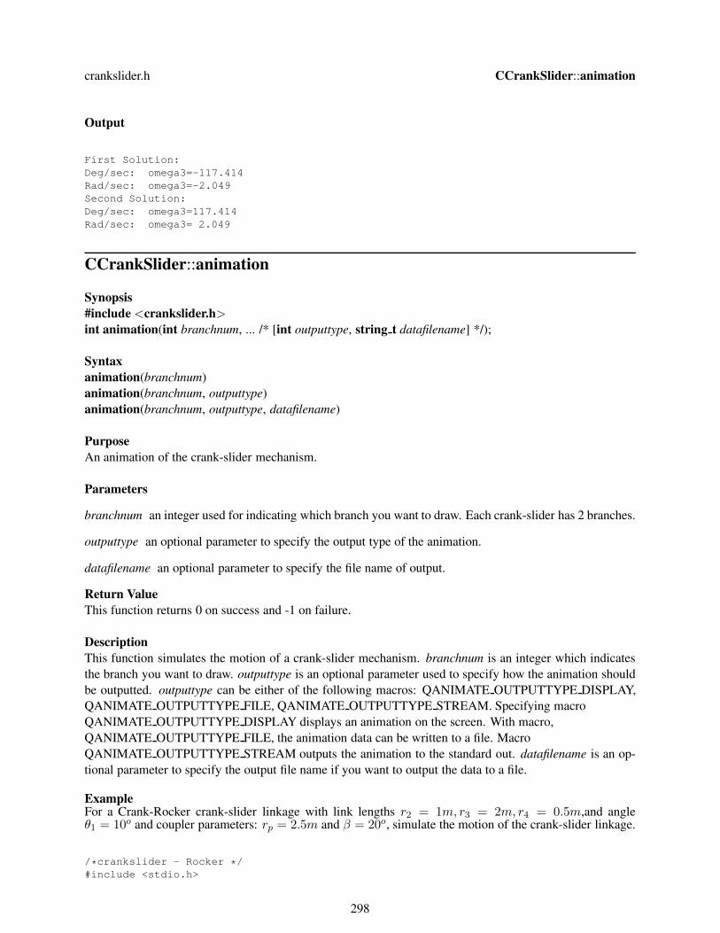
crankslider.h CCrankSlider::animation
Output
First Solution:
Deg/sec: omega3=-117.414
Rad/sec: omega3=-2.049
Second Solution:
Deg/sec: omega3=117.414
Rad/sec: omega3= 2.049
CCrankSlider::animation
Synopsis
#include <crankslider.h>int animation(int branchnum, ... /* [int outputtype, string t datafilename] */);
Syntax
animation(branchnum)
animation(branchnum, outputtype)
animation(branchnum, outputtype, datafilename)
Purpose
An animation of the crank-slider mechanism.
Parameters
branchnum an integer used for indicating which branch you want to draw. Each crank-slider has 2 branches.
outputtype an optional parameter to specify the output type of the animation.
datafilename an optional parameter to specify the file name of output.
Return Value
This function returns 0 on success and -1 on failure.
Description
This function simulates the motion of a crank-slider mechanism. branchnum is an integer which indicates
the branch you want to draw. outputtype is an optional parameter used to specify how the animation should
be outputted. outputtype can be either of the following macros: QANIMATE OUTPUTTYPE DISPLAY,
QANIMATE OUTPUTTYPE FILE, QANIMATE OUTPUTTYPE STREAM. Specifying macro
QANIMATE OUTPUTTYPE DISPLAY displays an animation on the screen. With macro,
QANIMATE OUTPUTTYPE FILE, the animation data can be written to a file. Macro
QANIMATE OUTPUTTYPE STREAM outputs the animation to the standard out. datafilename is an op-
tional parameter to specify the output file name if you want to output the data to a file.
ExampleFor a Crank-Rocker crank-slider linkage with link lengths r2 = 1m, r3 = 2m, r4 = 0.5m,and angleθ1 = 10o and coupler parameters: rp = 2.5m and β = 20o, simulate the motion of the crank-slider linkage.
/*crankslider - Rocker */
#include <stdio.h>
298
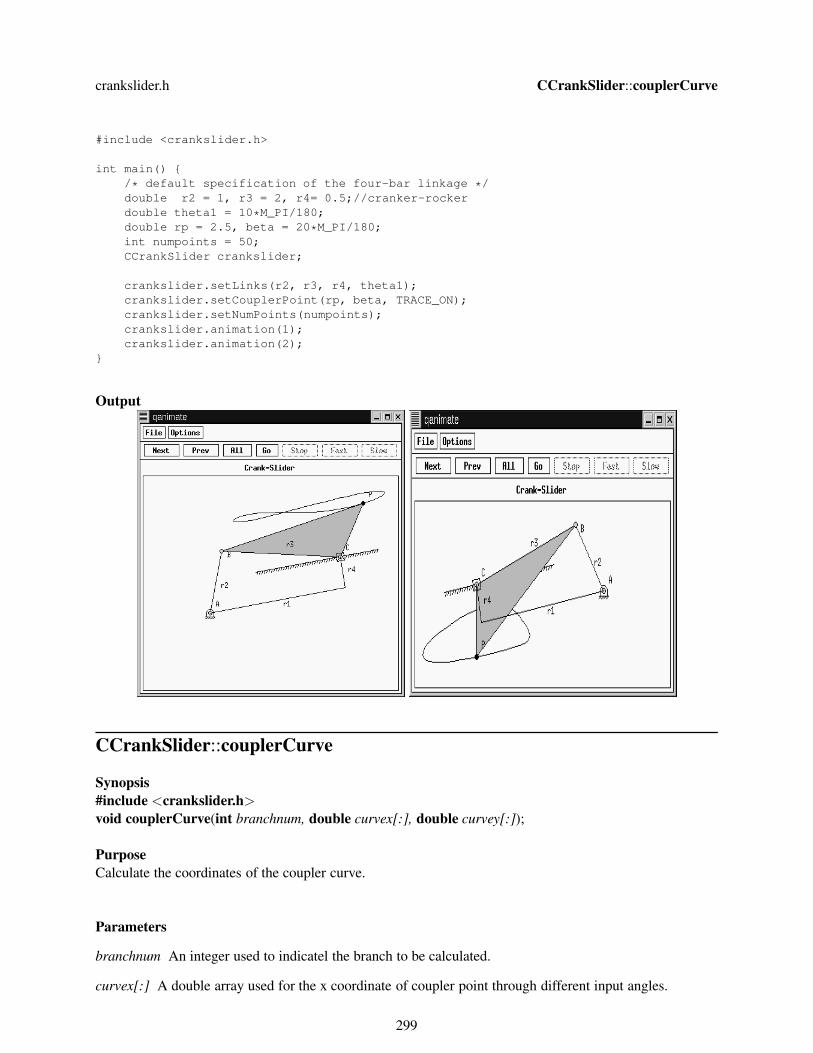
crankslider.h CCrankSlider::couplerCurve
#include <crankslider.h>
int main() {
/* default specification of the four-bar linkage */
double r2 = 1, r3 = 2, r4= 0.5;//cranker-rocker
double theta1 = 10*M_PI/180;
double rp = 2.5, beta = 20*M_PI/180;
int numpoints = 50;
CCrankSlider crankslider;
crankslider.setLinks(r2, r3, r4, theta1);
crankslider.setCouplerPoint(rp, beta, TRACE_ON);
crankslider.setNumPoints(numpoints);
crankslider.animation(1);
crankslider.animation(2);
}
Output
CCrankSlider::couplerCurve
Synopsis
#include <crankslider.h>void couplerCurve(int branchnum, double curvex[:], double curvey[:]);
Purpose
Calculate the coordinates of the coupler curve.
Parameters
branchnum An integer used to indicatel the branch to be calculated.
curvex[:] A double array used for the x coordinate of coupler point through different input angles.
299

crankslider.h CCrankSlider::couplerCurve
curvey[:] A double array used for the y coordinate of coupler point through different input angle.
Return Value
None.
Description
This function calculates the coupler point position by looping the input angle. curvex ,curvey are the coor-
dinate solutions of the coupler point positon.
ExampleFor a crank-slider with link lengths r2 = 1m, r3 = 2m, r4 = 0.5m, rp = 2.5m and angles θ1 = 0, andβ = 20o, plot the position curve of the coupler point.
#include <stdio.h>
#include <crankslider.h>
#include <chplot.h>
int main() {
CCrankSlider crankslider;
double r2 = 1, r3 = 2, r4 = 0.5; // crank-crank
double theta1 = 0;
double rp = 2.5, beta = 20*M_PI/180;
class CPlot pl;
double RetCurvex[50], RetCurvey[50];
crankslider.setLinks(r2, r3, r4, theta1);
crankslider.setCouplerPoint(rp, beta);
crankslider.setNumPoints(50);
// use coupler points plot curve
crankslider.couplerCurve(1, RetCurvex, RetCurvey);
plotxy(RetCurvex,RetCurvey,"Coupler curve ",
"Px (m)", "Py (m)", &pl);
pl.sizeRatio(-1);
pl.border(PLOT_BORDER_ALL, PLOT_ON);
pl.plotting();
}
Output
300
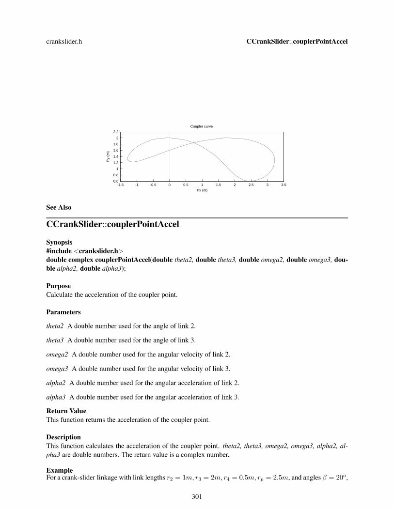
crankslider.h CCrankSlider::couplerPointAccel
0.6
0.8
1
1.2
1.4
1.6
1.8
2
2.2
-1.5 -1 -0.5 0 0.5 1 1.5 2 2.5 3 3.5
Py
(m)
Px (m)
Coupler curve
See Also
CCrankSlider::couplerPointAccel
Synopsis
#include <crankslider.h>double complex couplerPointAccel(double theta2, double theta3, double omega2, double omega3, dou-
ble alpha2, double alpha3);
Purpose
Calculate the acceleration of the coupler point.
Parameters
theta2 A double number used for the angle of link 2.
theta3 A double number used for the angle of link 3.
omega2 A double number used for the angular velocity of link 2.
omega3 A double number used for the angular velocity of link 3.
alpha2 A double number used for the angular acceleration of link 2.
alpha3 A double number used for the angular acceleration of link 3.
Return Value
This function returns the acceleration of the coupler point.
Description
This function calculates the acceleration of the coupler point. theta2, theta3, omega2, omega3, alpha2, al-
pha3 are double numbers. The return value is a complex number.
ExampleFor a crank-slider linkage with link lengths r2 = 1m, r3 = 2m, r4 = 0.5m, rp = 2.5m, and angles β = 20o,
301

crankslider.h CCrankSlider::couplerPointPos
and θ1 = 10o. Given the angle θ2, the angular velocity ω2 and the angular acceleration α2, calculate theacceleration of the coupler point for each circuit, respectively.
#include <math.h>
#include <crankslider.h>
int main() {
CCrankSlider crankslider;
double r2 = 1, r3 = 2, r4 = 0.5, theta1 = 10*M_PI/180;
double rp = 2.5, beta = 20*M_PI/180;
double theta2 = 70*M_PI/180;
double complex Ap[1:2];
double omega2 = 5; /* rad/sec */
double alpha2 =-5; /* rad/sec*sec */
double first_theta3, sec_theta3;
double first_omega3, sec_omega3;
double first_alpha3, sec_alpha3;
crankslider.setLinks(r2, r3, r4, theta1);
crankslider.setCouplerPoint(rp, beta);
crankslider.angularPos(theta2, first_theta3, sec_theta3);
first_omega3 = crankslider.angularVel(theta2, first_theta3, omega2);
sec_omega3 = crankslider.angularVel(theta2, sec_theta3, omega2);
first_alpha3 = crankslider.angularAccel(theta2, omega2, first_theta3, first_omega3,
alpha2);
sec_alpha3 = crankslider.angularAccel(theta2, omega2, sec_theta3, sec_omega3,
alpha2);
Ap[1] = crankslider.couplerPointAccel(theta2, first_theta3, omega2, first_omega3,
alpha2, first_alpha3);
Ap[2] = crankslider.couplerPointAccel(theta2, sec_theta3, omega2, sec_omega3, alpha2,
sec_alpha3);
printf("Circuit 1: \n CouplerAccleration: %f \n", Ap[1]);
printf("Circuit 2: \n CouplerAccleration: %f \n", Ap[2]);
}
Output
Circuit 1:
CouplerAccleration: complex(-17.383000,1.825762)
Circuit 2:
CouplerAccleration: complex(20.415886,-43.221212)
CCrankSlider::couplerPointPos
Synopsis
#include <crankslider.h>void couplerPointPos(double theta2, double complex &p1, double complex &p2);
Purpose
Calculate the position of the coupler point.
Parameters
theta2 A double number used for the input angle of link2.
302

crankslider.h CCrankSlider::couplerPointVel
p1 A double complex number for the first solution of the coupler point.
p2 A double complex number for the second solution of the coupler point. x.
Return Value
None.
Description
This function calculates the position of the coupler point. theta2 is the input angle. p1,p2 are the two so-
lutions of the coupler point position, respectively. Each is a complex number indicating the vector of the
coupler point.
Example
see CCrankSlider::angularPos().
CCrankSlider::couplerPointVel
Synopsis
#include <crankslider.h>double complex couplerPointVel(double theta2, double theta3, double omega2, double omega3);
Purpose
Calculate the velocity of the coupler point.
Parameters
theta2 A double number used for the angle of link 2.
theta3 A double number used for the angle of link 3.
omega2 A double number used for the angular velocity of link 2.
omega3 A double number used for the angular velocity of link 3.
Return Value
This function returns the vector of the coupler velocity.
Description
This function calculates the vector of the coupler velocity. theta2 is the angle of link2, theta3 is the angle
of link3. omega2 is the angular velocity of link2, omega3 is the angular velocity of link3. The vector ofthe
coupler point velocity is returned.
ExampleFor a crank-slider linkage with link lengths r2 = 1m, r3 = 2m, r4 = 0.5m, rp = 2.5m, and angles β = 20o,and θ1 = 10o. Given the angle θ2 and the angular velocity ω2, calculate the velocity of the coupler point foreach circuit, respectively.
303

crankslider.h CCrankSlider::displayPosition
#include <math.h>
#include <crankslider.h>
int main() {
CCrankSlider crankslider;
double r2 = 1, r3 = 2, r4 = 0.5, theta1 = 10*M_PI/180;
double rp = 2.5, beta = 20*M_PI/180;
double theta2 = 70*M_PI/180;
double complex Vp[1:2];
double omega2 = 5; /* rad/sec */
double first_theta3, sec_theta3;
double first_omega3, sec_omega3;
crankslider.setLinks(r2, r3, r4, theta1);
crankslider.setCouplerPoint(rp, beta);
crankslider.angularPos(theta2, first_theta3, sec_theta3);
first_omega3 = crankslider.angularVel(theta2, first_theta3, omega2);
sec_omega3 = crankslider.angularVel(theta2, sec_theta3, omega2);
Vp[1] = crankslider.couplerPointVel(theta2, first_theta3, omega2, first_omega3);
Vp[2] = crankslider.couplerPointVel(theta2, sec_theta3, omega2, sec_omega3);
printf("Circuit 1: \n CouplerVelocity: %f \n", Vp[1]);
printf("Circuit 2: \n CouplerVelocity: %f \n", Vp[2]);
}
Output
Circuit 1:
CouplerVelocity: complex(-3.668337,-1.297038)
Circuit 2:
CouplerVelocity: complex(-7.481037,3.246762)
CCrankSlider::displayPosition
Synopsis
#include <crankslider.h>int displayPosition(double theta2, double theta3, ... /* [int outputtype [, [char * filename]] */);
Syntax
displayPosition(theta2, theta3)
displayPosition(theta2, theta3, outputtype)
displayPosition(theta2, theta3, outputtype, filename)
Purpose
Given θ2 and θ3, display the current position of the crank-slider mechanism.
Parameters
theta2 θ2 angle.
theta3 θ3 angle.
outputtype an optional argument for the output type.
filename an optional argument for the output file name.
304

crankslider.h CCrankSlider::forceTorque
Return Value
This function returns 0 on success and -1 on failure.
Description
Given θ2 and θ3, display the current position of the crank-slider mechanism. outputtype is an optional
parameter used to specify how the output should be handled. It may be one of the following macros:
QANIMATE OUTPUTTYPE DISPLAY, QANIMATE OUTPUTTYPE FILE,
QANIMATE OUTPUTTYPE STREAM. QANIMATE OUTPUTTYPE DISPLAY outputs the figure to the
computer terminal. QANIMATE OUTPUTTYPE FILE writes the qanimate data onto a file.
QANIMATE OUTPUTTYPE STREAM outputs the qanimate data to the standard out stream. filename
is an optional parameter to specify the output file name.
ExampleA crank-slider mechanism has link lengths r2 = 1m, r3 = 2m, r4 = 0.5m, and θ1 = 10o. Given the an-gle θ2 = 45o, calculate the angular position θ3 and display the crank-slider mechanism in its current position.
#include <math.h>
#include <crankslider.h>
int main()
{
CCrankSlider crankslider;
double r2 = 1, r3 = 2, r4 = 0.5, theta1 = 10*M_PI/180;
double theta2 = 45*M_PI/180;
double theta3_1, theta3_2;
double complex rs_1, rs_2;
crankslider.setLinks(r2, r3, r4, theta1);
crankslider.angularPos(theta2, theta3_1, theta3_2);
crankslider.displayPosition(theta2, theta3_1);
crankslider.displayPosition(theta2, theta3_2);
return 0;
}
Output
CCrankSlider::forceTorque
Synopsis
#include <crankslider.h>
305

crankslider.h CCrankSlider::forceTorque
void forceTorque(double theta2, double theta3, double omega2, double omega3, double alpha2, double
alpha3, double Fl, double complex as, array double x[9]);
Purpose
Calculate the joint forces and input torque at a given point.
Parameters
theta2, theta3 Double numbers used for the angles of link2 and link3 respectively.
omega2, omega3 Double numbers used for the angular velocities of link2 and link3 respectively.
alpha2, alpha3 Double numbers used for the angular accelerations of link2 and link3 respectively.
Fl A double number used for the load force.
as A double number used for the acceleration of the slider.
x A double array used for forces and torque.
Return Value
None.
Description
This function calculates the joint forces and input torque for a given load torque. theta is a one-dimensional
array of size 4 for the angles of the links. omega is a one-dimensional array of size 4 for the angular veloci-
ties of the links. alpha is a one-dimensional array of size 4 for the angular acclerations of the links. Fl is the
load force. x contains the joint forces and input torque.
ExampleFor a crank-slider linkage with link lengths r2 = 1”, r3 = 2”, r4 = 0.5”, rp = 5”, and angles β = 20o, andθ1 = 10o. Given the angle θ2, the angular velocity ω2 and the angular acceleration α2, calculate the requiredtorque applied to the input link2 in order to achieve the constant angular velocity for link2. Also calculatethe joint forces exerted on the ground from links 1 and 4.
#include <math.h>
#include <crankslider.h>
int main() {
CCrankSlider crankslider;
double r2 = 1/12.0, r3 = 2/12.0, r4 = 0.5/12.0, theta1 = 10*M_PI/180;
double rp = 2.5/12.0, beta = 20*M_PI/180;
array double X[9];
double g = 32.2;
double rg2 = 2/12.0, rg3 = 6/12.0;
double m2 = 0.8/g, m3 = 2.4/g, m4 = 1.4/g;
double ig2 = 0.012/12.0, ig3 = 0.119/12.0, Fl=0;
double theta2 = 45*M_PI/180;
double omega2 = 5; /* rad/sec */
double alpha2 =-5; /* rad/sec*sec */
double first_theta3, sec_theta3;
double first_omega3, sec_omega3;
double first_alpha3, sec_alpha3;
306

crankslider.h CCrankSlider::forceTorques
double complex first_as, sec_as;
/* initialization of link parameters and
inertia properties */
crankslider.uscUnit(1);
crankslider.setLinks(r2, r3, r4, theta1);
crankslider.setCouplerPoint(rp, beta);
crankslider.setGravityCenter(rg2, rg3);
crankslider.setInertia(ig2, ig3);
crankslider.setMass(m2, m3, m4);
crankslider.angularPos(theta2, first_theta3, sec_theta3);
first_omega3 = crankslider.angularVel(theta2, first_theta3, omega2);
sec_omega3 = crankslider.angularVel(theta2, sec_theta3, omega2);
first_alpha3 = crankslider.angularAccel(theta2, omega2, first_theta3, first_omega3,
alpha2);
sec_alpha3 = crankslider.angularAccel(theta2, omega2, sec_theta3, sec_omega3,
alpha2);
first_as = crankslider.sliderAccel(theta2, first_theta3, omega2, first_omega3,
alpha2, first_alpha3);
sec_as = crankslider.sliderAccel(theta2, sec_theta3, omega2, sec_omega3, alpha2,
sec_alpha3);
crankslider.forceTorque(theta2, first_theta3, omega2, first_omega3, alpha2,
first_alpha3, Fl, first_as, X);
printf("first solution X = %.4f \n", X);
crankslider.forceTorque(theta2, sec_theta3, omega2, sec_omega3, alpha2, sec_alpha3,
Fl, sec_as, X);
printf("second solution X = %.4f \n", X);
}
Output
first solution X = 1.8977 -3.7569 1.8391 -4.6443 1.5499 -6.8617 -1.4595 8.2770 -0.2894
second solution X = 1.5349 -3.6799 1.4763 -4.5674 1.4706 -6.7348 -1.4354 8.1403 -0.2634
CCrankSlider::forceTorques
Synopsis
#include <crankslider.h>void forceTorques(int branchnum, double Fl,array double time[:], array double f12x[:], array double
f12y[:], array double f23x[:], array double f23y[:], array double f34x[:], array double f34y[:], array
double f14x[:], array double f14y[:], array double ts[:]);
Purpose
Calculate the joint forces and input torque in the valid range of motion.
Parameters
branchnum An integer number used for the branch that will be calculated.
307

crankslider.h CCrankSlider::forceTorques
Fl A double number for the load force.
time A double array to record time.
f12x, f12yble f23x, f23y, f34x, f34y, f14x, f14y Double arrays for forces.
ts A double array for input torque.
Return Value
None.
Description
This function calculates the joint forces and input torque in the valid range of motion. branchnum is the
branch which will be plotted. Fl is the load force. time is an array to record time. f12x, f12y, f23x, f23y,
f34x, f34y, f14x, f14y are arrays for forces. ts is a double array for input torque.
ExampleFor a crank-slider linkage with link lengths r2 = 1”, r3 = 2”, r4 = 0.5”, rp = 2.5”, and angles β = 20o,and θ1 = 10o. Given the angle θ2, use a loop to calculate the required torque applied to the input link2 inorder to achieve the constant angular velocity for link2. Also calculate the joint forces exerted on the groundfrom links 1 and 4.
#include <math.h>
#include <crankslider.h>
int main()
{
CCrankSlider crankslider;
double r2 = 1/12.0, r3 = 2/12.0, r4 = 0.5/12.0, theta1 = 10*M_PI/180;
double rp = 2.5/12.0, beta = 20*M_PI/180;
double g = 32.2;
double rg2 = 2/12.0, rg3 = 6/12.0;
double m2 = 0.8/g, m3 = 2.4/g, m4 = 1.4/g;
double ig2 = 0.012/12.0, ig3 = 0.119/12.0, Fl=0;
int numpoint = 50;
double omega2 = 5; /* constant omega2 */
array double time[numpoint], ts[numpoint];
array double f12x[numpoint], f12y[numpoint];
array double f23x[numpoint], f23y[numpoint];
array double f34x[numpoint], f34y[numpoint];
array double f14x[numpoint], f14y[numpoint];
int branchnum = 2;
int i;
class CPlot pl;
/* initialization of link parameters and
inertia properties */
crankslider.uscUnit(1);
crankslider.setLinks(r2, r3, r4, theta1);
crankslider.setCouplerPoint(rp, beta);
crankslider.setGravityCenter(rg2, rg3);
crankslider.setInertia(ig2, ig3);
crankslider.setMass(m2, m3, m4);
crankslider.setNumPoints(numpoint);
crankslider.setAngularVel(omega2);
308

crankslider.h CCrankSlider::forceTorques
crankslider.forceTorques(branchnum, Fl, time, f12x, f12y, f23x, f23y,
f34x, f34y, f14x, f14y, ts); // calculate the forces and torque
plotxy(time, ts, NULL, "time t (seconds)", "input torque Ts (ft-lbf)", &pl);
pl.border(PLOT_BORDER_ALL, PLOT_ON);
pl.plotting();
plotxy(time, f12x, NULL, "time t (seconds)", "Joint force (lbf)", &pl);
pl.data2D(time, f12y);
pl.data2D(time, f23x);
pl.data2D(time, f23y);
pl.data2D(time, f34x);
pl.data2D(time, f34y);
pl.data2D(time, f14x);
pl.data2D(time, f14y);
pl.legend("f12x",0);
pl.legend("f12y",1);
pl.legend("f23x",2);
pl.legend("f23y",3);
pl.legend("f34x",4);
pl.legend("f34y",5);
pl.legend("f14x",6);
pl.border(PLOT_BORDER_ALL, PLOT_ON);
pl.plotting();
}
Output
-0.4
-0.3
-0.2
-0.1
0
0.1
0.2
0.3
0.4
0 0.2 0.4 0.6 0.8 1 1.2 1.4
inpu
t tor
que
Ts
(ft-
lbf)
time t (seconds)
309

crankslider.h CCrankSlider::getJointLimits
-10
-5
0
5
10
15
0 0.2 0.4 0.6 0.8 1 1.2 1.4
Join
t for
ce (
lbf)
time t (seconds)
f12xf12yf23xf23yf34xf34yf14x
CCrankSlider::getJointLimits
Synopsis
#include <crankslider.h>int getJointLimits(double &inputmin, double &inputmax);
Purpose
Calculate the crank-slider linkage input and output joint limits.
Parameters
inputmin A double number used for the minimum input angle.
inputmax A double number used for the maximum input angle.
Return Value
If the crank can fully rotate, return 1, otherwise return FOURBAR INVALID.
Description
This function calculates the crank-slider linkage input limits. inputmin, inputmax are numbers for the limits
of the crank-slider linkage.
ExampleFor a crankslider linkage with link lengths r2 = 1m, r3 = 2m, r4 = 0.5m, and angle θ1 = 0, determine theinput limit and output limit for each circuit.
#include <math.h>
#include <crankslider.h>
int main() {
CCrankSlider crankslider;
double r2 = 1, r3 = 2, r4 = 0.5, theta1 = 0;
double inputlimitmin, inputlimitmax;
310

crankslider.h CCrankSlider::plotCouplerCurve
crankslider.setLinks(r2, r3, r4, theta1);
crankslider.getJointLimits(inputlimitmin, inputlimitmax);
printf("input Range:\n");
printf(" Lower limit: %7.2f\n",
inputlimitmin*180./M_PI);
printf(" Upper limit: %7.2f\n",
inputlimitmax*180./M_PI);
}
Output
input Range:
Lower limit: 0.00
Upper limit: 360.00
CCrankSlider::plotCouplerCurve
Synopsis
#include <crankslider.h>void plotCouplerCurve(CPlot *plot, int branchnum);
Syntax
plotCouplerCurve(&plot, branchnum)
Purpose
Plot the coupler curve.
Parameters
&plot A pointer to a CPlot class variable used to format the plot of the branch to be drawn.
branchnum An integer used for indicating the branch which you want to draw.
Return Value
None.
Description
This function plots the coupler curve. &plot is a pointer to a CPlot class variable used to format the plot of
the branch to be drawn. branchnum is an integer number which indicates the branch you want to draw.
Example
For a crank-slider linkage with link lengths r2 = 1m, r3 = 2m, r4 = 0.5m, rp = 2.5m, and angles θ1 = 0,
and β = 20o, plot the position curve of the coupler point.
#include <stdio.h>
#include <crankslider.h>
311

crankslider.h CCrankSlider::plotForceTorques
int main() {
CCrankSlider Slidercrank;
double r2 = 1, r3 = 2, r4 = 0.5;
double theta1 = 0;
double rp = 2.5, beta = 20*M_PI/180;
class CPlot plot;
Slidercrank.setLinks(r2, r3, r4, theta1);
Slidercrank.setCouplerPoint(rp, beta);
Slidercrank.setNumPoints(50);
Slidercrank.plotCouplerCurve(&plot, 1); //display a coupler curve
}
Output
0.6
0.8
1
1.2
1.4
1.6
1.8
2
2.2
-1.5 -1 -0.5 0 0.5 1 1.5 2 2.5 3 3.5
Py
(m)
Px (m)
Coupler Curve
CCrankSlider::plotForceTorques
Synopsis
#include <crankslider.h>void plotForceTorques(CPlot *plot, int branchnum, double Fl);
Syntax
plotForceTorques(&plot, branchnum,Fl)
Purpose
Plot the joint forces and input torque curves.
Parameters
&plot A CPlot class variable used to format the plot of the branch to be drawn.
branchnum An integer number used for idicating the branch which will be plotted.
Fl A double number for the load Force.
312

crankslider.h CCrankSlider::setCouplerPoint
Return Value
None.
Description
This function plots the joint forces and input torque curve. &plot is a CPlot class variable used to format the
plot of the branch to be drawn. branchnum is an integer for the branch which will be plotted.
ExampleA crank-slider linkage has link length r2 = 1”, r3 = 2”, r4 = 0.5”, and angle θ1 = 0o. Plot the jointforces and input torque versus time t, when the input link θ2 is rotated counterclockwise with a constantinput angular velocity.
#include <math.h>
#include <crankslider.h>
int main()
{
CCrankSlider crankslider;
double r2 = 1/12.0, r3 = 2/12.0, r4= 0.5/12.0;//cranker-rocker
double theta1 = 0;
double g = 32.2;
double rg2 = 2/12.0, rg3 = 6/12.0;
double m2 = 0.8/g, m3 = 2.4/g, m4 = 1.4/g;
double ig2 = 0.012/12.0, ig3 = 0.119/12.0, Fl=0;
int numpoint = 50;
double omega2 = 5; /* constant omega2 */
class CPlot plot;
/* initialization of link parameters and
inertia properties */
crankslider.uscUnit(1);
crankslider.setLinks(r2, r3, r4, theta1);
crankslider.setGravityCenter(rg2, rg3);
crankslider.setInertia(ig2, ig3);
crankslider.setMass(m2, m3, m4);
crankslider.setNumPoints(numpoint);
crankslider.setAngularVel(omega2);
crankslider.plotForceTorques(&plot,1,Fl); //first branch
}
Output
313

crankslider.h CCrankSlider::setGravityCenter
-10
-8
-6
-4
-2
0
2
4
6
8
10
12
0 0.2 0.4 0.6 0.8 1 1.2 1.4
forc
e (lb
f)/to
rque
(lb
f-ft)
time t (seconds)
F12_xF12_yF23_xF23_yF34_xF34_yF14_xF14_y
Ts
CCrankSlider::setCouplerPoint
Synopsis
#include <crankslider.h>void setCouplerPoint(double rp, beta, ... /* [int trace] */);
Syntax
setCouplerPoint(rp, beta)
setCouplerPoint(rp, beta, trace)
Purpose
Set parameters for the coupler point.
Parameters
rp A double number used for rp.
beta A double number for beta.
trace An optional parameter of int type specifying either macro TRACE OFF or TRACE ON to indicte
whether the coupler curve should be traced during animation.
Return Value
None.
Description
This function sets the parameters of the coupler point.
Example
see CCrankSlider::plotCouplerCurve().
CCrankSlider::setGravityCenter
314

crankslider.h CCrankSlider::setAngularVel
Synopsis
#include <crankslider.h>void setGravityCenter(double rg2, double rg3);
Purpose
Set the mass center parameters of the links.
Parameters
rg2 A double number used for the distance from joint A0 to the center of gravity of link 2.
rg3 A double number used for the distance from joint A to the center of gravity of link 3.
Return Value
None.
Description
This function sets parameters for mass centers of links.
Example
see CCrankSlider::plotForceTorques().
CCrankSlider::setInertia
Synopsis
#include <crankslider.h>void setInertia(double ig2, double ig3);
Purpose
Set inertia parameters of the links.
Parameters
ig2 A double number used for the inertia of link 2.
ig3 A double number used for the inertia of link 3.
Return Value
None.
Description
This function sets inertia parameters of the links.
Example
see CCrankSlider::plotForceTorques().
CCrankSlider::setAngularVel
Synopsis
#include <crankslider.h>
315

crankslider.h CCrankSlider::setMass
void setAngularVel(double omega2);
Purpose
Set the constant angular velocity of link2.
Parameters
omega2 A double number used for the constant input angular velocity of link2.
Return Value
None.
Description
This function sets the constant angular velocity of link2. It is used in conjunction with member functions
forceTorques() and plotForceTorques().
Example
see CCrankSlider::plotForceTorques().
CCrankSlider::setLinks
Synopsis
#include <crankslider.h>int setLinks(double r2, double r3, double r4, double theta1);
Purpose
Set the lengths of the links.
Parameters
r2,r3,r4 Double numbers used for the lengths of each link.
theta1 A double number representing the angle between link1 and horizontal.
Return Value
This function returns 0 on success and -1 on failure.
Description
This function sets the lengths of links and detects if the lengths can construct a crank-slider mechanism. If
not, return -1.
Example
see CCrankSlider::plotCouplerCurve().
CCrankSlider::setMass
Synopsis
#include <crankslider.h>void setMass(double m2, double m3, double m4);
316

crankslider.h CCrankSlider::sliderAccel
Purpose
Set the mass of each link.
Parameters
m2,m3,m4 Double numbers used for the mass of the links.
Return Value
None.
Description
This function sets the masses of links.
Example
see CCrankSlider::plotForceTorques().
CCrankSlider::setNumPoints
Synopsis
#include <crankslider.h>void setNumPoints(int numpoints);
Purpose
Set the number of points for the animation and the coupler curve.
Parameters
numpoints An integer number used for the number of points.
Return Value
None.
Description
This function sets the number of points for the animation and the coupler curve plot.
Example
see CCrankSlider::animation().
CCrankSlider::sliderAccel
Synopsis
#include <crankslider.h>double sliderAccel(double theta2, double theta3, double omega2, double omega3, double alpha2, double
alpha3);
Purpose
Given the angular acceleration of link2, calculate the acceleration of the slider.
Parameters
317

crankslider.h CCrankSlider::sliderAccel
theta2, theta3 Double numbers indicating the angular position of link2 and link 3, respective.
omega2, omega3 Double numbers indicating the angular velocity of link2 and link3, respective.
alpha2, alpha3 Double numbers indicating the angular acceleration of link2 and link3, respective.
Return Value
This function returns the acceleration of the slider.
Description
Given the angular acceleration of one link, this function calculates the acceleration of slider. theta2, theta3
are double numbers which store the angle of link2 and link3, respective. omega2, omega3 are double num-
bers which store the angular velocity of link2 and link3, respective. alpha2, alpha3 are double numbers
which store the angular acceleration of link2. The returned value is the result of calculation.
ExampleA crank-slider linkage has link lengths r2 = 1m, r3 = 2m, r4 = 0.5m, and angle θ1 = 10o. Given theangle θ2, the angular velocity ω2 and the angular acceleration α2, calculate the acceleration of the slider foreach circuit.
#include <math.h>
#include <crankslider.h>
int main() {
CCrankSlider crankslider;
double r2 = 1, r3 = 2, r4 = 0.5, theta1 = 10*M_PI/180;
double rp = 2.5, beta = 20*M_PI/180;
double theta2 = 70*M_PI/180;
double complex As[1:2];
double omega2 = 5; /* rad/sec */
double alpha2 =-5; /* rad/sec*sec */
double first_theta3, sec_theta3;
double first_omega3, sec_omega3;
double first_alpha3, sec_alpha3;
crankslider.setLinks(r2, r3, r4, theta1);
crankslider.setCouplerPoint(rp, beta);
crankslider.angularPos(theta2, first_theta3, sec_theta3);
first_omega3 = crankslider.angularVel(theta2, first_theta3, omega2);
sec_omega3 = crankslider.angularVel(theta2, sec_theta3, omega2);
first_alpha3 = crankslider.angularAccel(theta2, omega2, first_theta3,
first_omega3, alpha2);
sec_alpha3 = crankslider.angularAccel(theta2, omega2, sec_theta3, sec_omega3,
alpha2);
As[1] = crankslider.sliderAccel(theta2, first_theta3, omega2, first_omega3,
alpha2, first_alpha3);
As[2] = crankslider.sliderAccel(theta2, sec_theta3, omega2, sec_omega3,
alpha2, sec_alpha3);
printf("Circuit 1: \n SliderAccleration: %f \n", As[1]);
printf("Circuit 2: \n SliderAccleration: %f \n", As[2]);
}
Output
318

crankslider.h CCrankSlider::sliderPos
Circuit 1:
SliderAcceleration: complex(-6.857122, -1.209097)
Circuit 2:
SliderAcceleration: complex(-9.234371, -1.628269)
CCrankSlider::sliderPos
Synopsis
#include <crankslider.h>void sliderPos(double theta2, double complex &first solution, double complex &sec solution,);
Purpose
Given the angular velocity of link2, calculate the position of the slider.
Parameters
theta2 Double numbers used for the input angle of link2.
first solution Double complex number used to store the first solution of the slider position.
sec solution Double complex number used to store the second solution of the slider position.
Return Value
No return value.
Description
Given the angular position of link2, this function calculates the position of the slider. theta2 is a double
number for the position of link 2. first solution, sec solution are double complex numbers for the two pos-
sible solutions to the position of the slider.
ExampleA crank-slider linkage has link lengths r2 = 1m, r3 = 2m, r4 = 0.5m, and angle θ1 = 10o. Given theangle θ2, determine the position of the slider for each circuit.
#include <math.h>
#include <crankslider.h>
int main() {
CCrankSlider crankslider;
double r2 = 1, r3 = 2, r4 = 0.5, theta1 = 10*M_PI/180;
double rp = 2.5, beta = 20*M_PI/180;
double theta2 = 70*M_PI/180;
double complex Ps[1:2];
double first_theta3, sec_theta3;
crankslider.setLinks(r2, r3, r4, theta1);
crankslider.setCouplerPoint(rp, beta);
crankslider.angularPos(theta2, first_theta3, sec_theta3);
crankslider.sliderPos(theta2, Ps[1], Ps[2]);
printf("Circuit 1: \n Slider Position: %f \n", Ps[1]);
printf("Circuit 2: \n Slider Position: %f \n", Ps[2]);
return 0;
}
319

crankslider.h CCrankSlider::sliderVel
Output
Circuit 1:
Slider Position: complex(2.341929,0.920659)
Circuit 2:
Slider Position: complex(-1.530770,0.237797)
CCrankSlider::sliderVel
Synopsis
#include <crankslider.h>double sliderVel(double theta2, double theta3, double omega2, double omega3);
Purpose
Given the angular velocity of link2, calculate the velocity of the slider.
Parameters
theta2, theta3 Double numbers used for the input angles of link2 and link3 respectively.
omega2, omega3 Double numbers used for the angular velocity of link2 and link3 respectively.
Return Value
This function returns the velocity of the slider.
Description
Given the angular velocity of link2, this function calculates the velocity of the slider. theta2, theta3 are
double numbers for link positions. omega2, omega3 are double numbers for the angular velocities of links.
ExampleA crank-slider linkage has link lengths r2 = 1m, r3 = 2m, r4 = 0.5m, and angle θ1 = 10o. Given theangle θ2 and the angular velocity ω2, determine the slider velocity for each circuit.
#include <math.h>
#include <crankslider.h>
int main() {
CCrankSlider crankslider;
double r2 = 1, r3 = 2, r4 = 0.5, theta1 = 10*M_PI/180;
double rp = 2.5, beta = 20*M_PI/180;
double theta2 = 70*M_PI/180;
double complex Vs[1:2];
double omega2 = 5; /* rad/sec */
double first_theta3, sec_theta3;
double first_omega3, sec_omega3;
crankslider.setLinks(r2, r3, r4, theta1);
crankslider.setCouplerPoint(rp, beta);
crankslider.angularPos(theta2, first_theta3, sec_theta3);
first_omega3 = crankslider.angularVel(theta2, first_theta3, omega2);
sec_omega3 = crankslider.angularVel(theta2, sec_theta3, omega2);
Vs[1] = crankslider.sliderVel(theta2, first_theta3, omega2, first_omega3);
Vs[2] = crankslider.sliderVel(theta2, sec_theta3, omega2, sec_omega3);
320

crankslider.h CCrankSlider::transAngle
printf("Circuit 1: \n SliderVelocity: %f \n", Vs[1]);
printf("Circuit 2: \n SliderVelocity: %f \n", Vs[2]);
}
Output
Circuit 1:
SliderVelocity: complex(-4.722665, -0.832733)
Circuit 2:
SliderVelocity: complex(-3.806022, -0.671104)
CCrankSlider::transAngle
Synopsis
#include <crankslider.h>void transAngle(double &gamma1, double &gamma2, double theta2);
Purpose
Given the position of the input link, calculate the transmission angle.
Parameters
gamma1 A double number used for the first solution.
gamma2 A double number used for the second solution.
theta2 A double number used for the angular positon of link2.
Return Value
None.
Description
Given the position of the input link, this function calculates the transmission angle.ExampleA crank-slider linkage has link lengths r2 = 1m, r3 = 2m, r4 = 0.5m, and angle θ1 = 10o. Given theangle θ2, calculate the transmission angle for each circuit, respectively.
#include <math.h>
#include <stdio.h>
#include <crankslider.h>
int main() {
double r[1:4], theta1, theta2;
double gamma1, gamma2;
CCrankSlider crankslider;
/* default specification of the four-bar linkage */
r[2] = 1; r[3] = 2; r[4] = 0.5;
theta1 = 10*M_PI/180; theta2=45*M_PI/180;
printf("Results: Interactive Four-Bar Linkage Transmission Angle Analysis\n\n");
321

crankslider.h CCrankSlider::uscUnit
crankslider.setLinks(r[2], r[3], r[4], theta1);
crankslider.transAngle(gamma1, gamma2, theta2);
printf("\n Circuit 1: Transmission Angle\n\n");
printf("\tDegrees:\t gamma=%6.3f \n",gamma1*180/M_PI);
printf("\tRadians:\t gamma=%6.4f \n",gamma1);
printf("\n Circuit 2: Transmission Angle\n\n");
printf("\tDegrees:\t gamma=%6.3f \n",gamma2*180/M_PI);
printf("\tRadians:\t gamma=%6.4f \n",gamma2);
}
Output
Results: Interactive Four-Bar Linkage Transmission Angle Analysis
Circuit 1: Transmission Angle
Degrees: gamma=87.892
Radians: gamma=1.5340
Circuit 2: Transmission Angle
Degrees: gamma=-87.892
Radians: gamma=-1.5340
CCrankSlider::uscUnit
Synopsis
#include <crankslider.h>void uscUnit(bool unit);
Purpose
Specify the use of SI or US Customary units in analysis.
Parameters
unit A boolean argument, where true indicates US Customary units are desired and false indicates SI
units.
Return Value
None.
Description
This function specifies the whether SI or US Customary units are used.If unit = true, then US Cus-
tomary units are used; otherwise, SI units are used. By default, SI units are assumed. This member function
shall be called prior any other member function calls.
322

Appendix D
Class CGearedFivebar
CGearedFivebar
The header file fivebar.h includes header file linkage.h. The header file fivebar.h also contains a declaration
of class CGearedFivebar. The CGearedFivebar class provides a means to analyze geared fivebar linkage
within a Ch language environment.
Public Data
None.
Public Member Functions
Functions Descriptions
angularAccel Given the angular acceleration of one link, calculate the angular acceleration of other
links.
angularPos Given the angle of one link, caculate the angle of other links.
angularVel Given the angular velocity of one link, calculate the angular velocity of other links.
animation Fourbar linkage animation.
couplerCurve Calculate the coordinates of the coupler curve.
couplerPointAccel Calculate the acceleration of the coupler point.
couplerPointPos Calculate the position of the coupler point.
couplerPointVel Calculate the velocity of the coupler point.
323

Chapter D: Geared-Fivebar Linkage <fivebar.h> CGearedFivebar::angularAccel
displayPosition Display the geared fivebar positions.
plotCouplerCurve Plot the coupler curves.
setCouplerPoint Set parameters for the coupler point.
setAngularVel Set constant angular velocity of linkage 2.
setLinks Set lengths of links.
setNumPoints Set number of points for animation and plot coupler curve.
uscUnit Specify the use of SI or US Customary units.
See Also
CGearedFivebar::angularAccel
Synopsis
#include <fivebar.h>void angularAccel(double theta[1:5], double omega[1:5], double alpha[1:5]);
Purpose
Given the angular acceleration of the input link, calculate the angular accelerations of other links.
Parameters
theta An array of double data type with angles of links.
omega An array of double data type with angular velocities of links.
alpha An array of double data type with angular accelerations of links.
Return Value
None.
Description
Given the angular acceleration of the input link, this function calculates the angular acceleration of the re-
maining moving links of the geared fivebar. theta is a one-dimensional array of size 5 which stores the angle
of each link. omega is a one-dimensional array of size 5 which stores the angular velocity of each link.
alpha is a one-dimensional array of size 5 which stores the angular acceleration of each link. The result of
calculation is stored in array alpha.
ExampleA geared fivebar linkage has parameters r1 = 7m, r2 = 5m, r3 = 10m, r4 = 10m, r5 = 2m, θ1 = 10o,λ = −2.5, φ = 35o. Given the angle θ2, the angular velocity ω2 and the angular acceleration α2, calculatethe angular accelerations of the other links.
/*****************************************************************
* This example is for calculating the angular acceleration of *
* link3 and link4. *
*****************************************************************/
#include <fivebar.h>
324

Chapter D: Geared-Fivebar Linkage <fivebar.h> CGearedFivebar::angularAccel
int main()
{
double r[1:5],
theta_1[1:5], theta_2[1:5],
omega_1[1:5], omega_2[1:5],
alpha_1[1:5], alpha_2[1:5],
phi, lambda;
double complex P[1:2], Vp[1:2], Ap[1:2];
CGearedFivebar gearedbar;
/* Setup geared fivebar linkage. */
r[1] = 7; r[2] = 5; r[3] = 10; r[4] = 10; r[5] = 2;
phi = 35*M_PI/180; lambda = -2.5;
theta_1[1] = 10*(M_PI/180); theta_2[1] = 10*(M_PI/180);
theta_1[2] = 50*(M_PI/180); theta_2[2] = 50*(M_PI/180);
omega_1[2] = 5*(M_PI/180); omega_2[2] = 5*(M_PI/180);
alpha_1[2] = 0; alpha_2[2] = 0;
theta_1[5] = lambda*theta_1[2] + phi;
theta_2[5] = lambda*theta_2[2] + phi;
if(theta_1[5] < -M_PI)
{
theta_1[5] += 2*M_PI;
theta_2[5] += 2*M_PI;
}
if(theta_1[5] > M_PI)
{
theta_1[5] -= 2*M_PI;
theta_2[5] -= 2*M_PI;
}
/* Perform geared fivebar linkage analysis. */
gearedbar.setLinks(r[1], r[2], r[3], r[4], r[5], theta_1[1]);
gearedbar.setLambda(lambda);
gearedbar.setPhi(phi);
gearedbar.angularPos(theta_1, theta_2);
gearedbar.angularVel(theta_1, omega_1);
gearedbar.angularVel(theta_2, omega_2);
gearedbar.angularAccel(theta_1, omega_1, alpha_1);
gearedbar.angularAccel(theta_2, omega_2, alpha_2);
/* print results on screen */
printf("1st Circuit:\n");
printf("\talpha3 = %.3f rad/secˆ2 (%.2f deg/secˆ2)\n", alpha_1[3],
alpha_1[3]*(180/M_PI));
printf("\talpha4 = %.3f rad/secˆ2 (%.2f deg/secˆ2)\n\n", alpha_1[4],
alpha_1[4]*(180/M_PI));
printf("2nd Circuit:\n");
printf("\talpha3 = %.3f rad/secˆ2 (%.2f deg/secˆ2)\n", alpha_2[3],
alpha_2[3]*(180/M_PI));
printf("\talpha4 = %.3f rad/secˆ2 (%.2f deg/secˆ2)\n\n", alpha_2[4],
alpha_2[4]*(180/M_PI));
return 0;
}
Output
1st Circuit:
alpha3 = 0.003 rad/secˆ2 (0.20 deg/secˆ2)
alpha4 = -0.001 rad/secˆ2 (-0.04 deg/secˆ2)
325

Chapter D: Geared-Fivebar Linkage <fivebar.h> CGearedFivebar::angularPos
2nd Circuit:
alpha3 = 0.013 rad/secˆ2 (0.72 deg/secˆ2)
alpha4 = 0.020 rad/secˆ2 (1.17 deg/secˆ2)
CGearedFivebar::angularPos
Synopsis
#include <fivebar.h>void angularPos(double theta 1[1:5], double theta 2[1:5]);
Purpose
Given the angle of the input link, calculate the angles of other links.
Parameters
theta 1 A double array with of size 5 for the first solution.
theta 2 A double array of size 5 for the second solution.
Return Value
None.
Description
Given the angular position of one link of a fivebar linkage, this function computes the angular positions of
the remaining moving links. theta 1 is a one-dimensional array of size 5 which stores the first solution of the
angular positions. theta 2 is a one-dimensional array of size 5 which stores the second solution of angular
positions.
ExampleA geared fivebar linkage has parameters r1 = 7m, r2 = 5m, r3 = 10m, r4 = 10m, r5 = 2m, θ1 = 10o,λ = −2.5, and φ = 35o. Given the angle θ2, calculate the angular positions of the other links for eachrespective circuit.
/*************************************************************
* This example is for calculating the angular position of *
* link3 and link4. *
*************************************************************/
#include <fivebar.h>
int main()
{
double r[1:5],
theta_1[1:5], theta_2[1:5],
phi, lambda;
CGearedFivebar gearedbar;
/* Setup geared fivebar linkage. */
r[1] = 7; r[2] = 5; r[3] = 10; r[4] = 10; r[5] = 2;
phi = 35*M_PI/180; lambda = -2.5;
theta_1[1] = 10*(M_PI/180); theta_2[1] = 10*(M_PI/180);
326

Chapter D: Geared-Fivebar Linkage <fivebar.h> CGearedFivebar::angularPos
theta_1[2] = 50*(M_PI/180); theta_2[2] = 50*(M_PI/180);
theta_1[5] = lambda*theta_1[2] + phi;
theta_2[5] = lambda*theta_2[2] + phi;
if(theta_1[5] < -M_PI)
{
theta_1[5] += 2*M_PI;
theta_2[5] += 2*M_PI;
}
if(theta_1[5] > M_PI)
{
theta_1[5] -= 2*M_PI;
theta_2[5] -= 2*M_PI;
}
/* Perform geared fivebar linkage analysis. */
gearedbar.setLinks(r[1], r[2], r[3], r[4], r[5], theta_1[1]);
gearedbar.setLambda(lambda);
gearedbar.setPhi(phi);
gearedbar.angularPos(theta_1, theta_2);
/* May run into problem with theta4 being in opposite quadrant. */
theta_1[4] += M_PI; theta_2[4] += M_PI;
if(theta_1[4] < -M_PI)
theta_1[4] += 2*M_PI;
if(theta_1[4] > M_PI)
theta_1[4] -= 2*M_PI;
if(theta_2[4] < -M_PI)
theta_2[4] += 2*M_PI;
if(theta_2[4] > M_PI)
theta_2[4] -= 2*M_PI;
/* print results on screen */
printf("1st Circuit:\n");
printf("\ttheta3 = %.3f radians (%.2f degrees)\n", theta_1[3],
theta_1[3]*(180/M_PI));
printf("\ttheta4 = %.3f radians (%.2f degrees)\n", theta_1[4],
theta_1[4]*(180/M_PI));
printf("\ttheta5 = %.3f radians (%.2f degrees)\n\n", theta_1[5],
theta_1[5]*(180/M_PI));
printf("2nd Circuit:\n");
printf("\ttheta3 = %.3f radians (%.2f degrees)\n", theta_2[3],
theta_2[3]*(180/M_PI));
printf("\ttheta4 = %.3f radians (%.2f degrees)\n", theta_2[4],
theta_2[4]*(180/M_PI));
printf("\ttheta5 = %.3f radians (%.2f degrees)\n\n", theta_2[5],
theta_2[5]*(180/M_PI));
return 0;
}
Output
1st Circuit:
theta3 = 0.374 radians (21.40 degrees)
theta4 = -2.169 radians (-124.27 degrees)
theta5 = -1.571 radians (-90.00 degrees)
2nd Circuit:
theta3 = -2.169 radians (-124.27 degrees)
327

Chapter D: Geared-Fivebar Linkage <fivebar.h> CGearedFivebar::angularVel
theta4 = 0.374 radians (21.40 degrees)
theta5 = -1.571 radians (-90.00 degrees)
CGearedFivebar::angularVel
Synopsis
#include <fivebar.h>void angularVel(double theta[1:5], double omega[1:5]);
Purpose
Given the angular velocity of one link, calculate the angular velocities of other links.
Parameters
theta A double array used for the input angle of links.
omega A double array used for the angular velocities of links.
Return Value
None.
Description
Given the angular velocity of one link, this function calculates the angular velocities of the remaining two
moving links of the fivebar. theta is an array for link positions. omega is an array for angular velocity of
links.
ExampleA geared fivebar linkage has parameters r1 = 7m, r2 = 5m, r3 = 10m, r4 = 10m, r5 = 2m, θ1 = 10o,λ = −2.5, and φ = 35o. Given the angle θ2 and angular velocity ω2, calculate the angular velocities ω3, ω4of link3, and link4 for each circuit, respectively.
/*************************************************************
* This example is for calculating the angular velocity of *
* link3 and link4. *
*************************************************************/
#include <fivebar.h>
int main()
{
double r[1:5],
theta_1[1:5], theta_2[1:5],
omega_1[1:5], omega_2[1:5],
phi, lambda;
CGearedFivebar gearedbar;
/* Setup geared fivebar linkage. */
r[1] = 7; r[2] = 5; r[3] = 10; r[4] = 10; r[5] = 2;
phi = 35*M_PI/180; lambda = -2.5;
theta_1[1] = 10*(M_PI/180); theta_2[1] = 10*(M_PI/180);
theta_1[2] = 50*(M_PI/180); theta_2[2] = 50*(M_PI/180);
omega_1[2] = 5*(M_PI/180); omega_2[2] = 5*(M_PI/180);
328

Chapter D: Geared-Fivebar Linkage <fivebar.h> CGearedFivebar::animation
theta_1[5] = lambda*theta_1[2] + phi;
theta_2[5] = lambda*theta_2[2] + phi;
if(theta_1[5] < -M_PI)
{
theta_1[5] += 2*M_PI;
theta_2[5] += 2*M_PI;
}
if(theta_1[5] > M_PI)
{
theta_1[5] -= 2*M_PI;
theta_2[5] -= 2*M_PI;
}
/* Perform geared fivebar linkage analysis. */
gearedbar.setLinks(r[1], r[2], r[3], r[4], r[5], theta_1[1]);
gearedbar.setLambda(lambda);
gearedbar.setPhi(phi);
gearedbar.angularPos(theta_1, theta_2);
gearedbar.angularVel(theta_1, omega_1);
gearedbar.angularVel(theta_2, omega_2);
/* print results on screen */
printf("1st Circuit:\n");
printf("\tomega3 = %.3f rad/sec (%.2f deg/sec)\n", omega_1[3], omega_1[3]*(180/M_PI));
printf("\tomega4 = %.3f rad/sec (%.2f deg/sec)\n", omega_1[4], omega_1[4]*(180/M_PI));
printf("2nd Circuit:\n");
printf("\tomega3 = %.3f rad/sec (%.2f deg/sec)\n", omega_2[3], omega_2[3]*(180/M_PI));
printf("\tomega4 = %.3f rad/sec (%.2f deg/sec)\n", omega_2[4], omega_2[4]*(180/M_PI));
return 0;
}
Output
1st Circuit:
omega3 = -0.051 rad/sec (-2.94 deg/sec)
omega4 = 0.109 rad/sec (6.25 deg/sec)
2nd Circuit:
omega3 = -0.035 rad/sec (-2.01 deg/sec)
omega4 = 0.036 rad/sec (2.05 deg/sec)
CGearedFivebar::animation
Synopsis
#include <fivebar.h>int animation(int branchnum, ... /* [intoutputtype, string t datafilename] */);
Syntax
animation(branchnum)
animation(branchnum, outputtype)
animation(branchnum, outputtype, datafilename)
Purpose
An animation of a geared fivebar mechanism.
329

Chapter D: Geared-Fivebar Linkage <fivebar.h> CGearedFivebar::animation
Parameters
branchnum an integer used for indicating which branch you want to draw.
outputtype an optional parameter to specify the output type of the animation.
datafilename an optional parameter to specify the file name of output.
Return Value
This function returns 0 on success and -1 on failure.
Description
This function simulates the motion of a fivebar mechanism. branchnum is an integer number which indicates
the branch you want to draw. outputtype is an optional parameter used to specify how the animation should
be outputted. outputtype can be either of the following macros:
QANIMATE OUTPUTTYPE DISPLAY, QANIMATE OUTPUTTYPE FILE,
QANIMATE OUTPUTTYPE STREAM. QANIMATE OUTPUTTYPE DISPLAY creates an animation on
the screen. QANIMATE OUTPUTTYPE FILE writes the animation data onto a file, and
QANIMATE OUTPUTTYPE STREAM outputs the animation to the standard out. datafilename is an op-
tional parameter to specify the file name of output if you want to output the data to a file.
Example 1For a geared fivebar linkage with parameters r1 = 7m, r2 = 5m, r3 = 10m, r4 = 10m, r5 = 2m, θ1 = 0,λ = −2.5, φ = 35o, ω2 = 5rad/sec, and α2 = 0, simulate the motion of the fivebar linkage. Also trace themotion of the coupler point attached to link 3 with parameters rp = 5m and β = 45o.
/***************************************************
* This example is to simulate the motion of the *
* geared fivebar linkage. *
***************************************************/
#include <fivebar.h>
int main()
{
double r[1:5],
theta_1[1:5], theta_2[1:5],
rp, beta, phi, lambda;
double omega2, alpha2;
CGearedFivebar gearedbar;
/* Setup geared fivebar linkage. */
r[1] = 7; r[2] = 5; r[3] = 10; r[4] = 10; r[5] = 2;
rp = 5; beta = 45*(M_PI/180);
phi = 35*M_PI/180; lambda = -2.5;
theta_1[1] = 10*(M_PI/180); theta_2[1] = 10*(M_PI/180);
theta_1[2] = 50*(M_PI/180); theta_2[2] = 50*(M_PI/180);
theta_1[5] = lambda*theta_1[2] + phi;
theta_2[5] = lambda*theta_2[2] + phi;
if(theta_1[5] < -M_PI)
{
theta_1[5] += 2*M_PI;
theta_2[5] += 2*M_PI;
}
330

Chapter D: Geared-Fivebar Linkage <fivebar.h> CGearedFivebar::couplerCurve
if(theta_1[5] > M_PI)
{
theta_1[5] -= 2*M_PI;
theta_2[5] -= 2*M_PI;
}
/* Perform geared fivebar linkage analysis. */
gearedbar.setLinks(r[1], r[2], r[3], r[4], r[5], theta_1[1]);
gearedbar.setCouplerPoint(COUPLER_LINK3, rp, beta, TRACE_ON);
gearedbar.setLambda(lambda);
gearedbar.setPhi(phi);
gearedbar.setNumPoints(50);
gearedbar.animation(1);
gearedbar.animation(2);
return 0;
}
Output
CGearedFivebar::couplerCurve
Synopsis
#include <fivebar.h>void couplerCurve(int couplerLink, int branchnum, double curvex[:], double curvey[:]);
Purpose
Calculate the coordinates of the coupler curve.
Parameters
couplerLink An int value specifying a macro to indicate which link the coupler is attached to.
branchnum An integer number used for the branch which will be calculated.
331

Chapter D: Geared-Fivebar Linkage <fivebar.h> CGearedFivebar::couplerCurve
curvex[:] A double array used for the x coordinate of the coupler point with different input angle.
curvey[:] A double array used for the y coordinate of the coupler point with different input angle.
Return Value
None.
Description
This function calculates the coupler point position while looping the input angle. curvex ,curvey is the solu-
tion of the coupler point positon.
ExampleFor a geared fivebar linkage, given the lengths of the links and the fact that the coupler is attached to link 3,draw the position curve of the coupler point for each respective circuit.
/**************************************************************
* This example is for determining the coupler curve of the *
* geared fivebar linkage. *
**************************************************************/
#include <fivebar.h>
int main()
{
double r[1:5],
theta1,
rp, beta, phi, lambda;
int numpoint = 100;
double RetCurvex_1[numpoint], RetCurvey_1[numpoint];
double RetCurvex_2[numpoint], RetCurvey_2[numpoint];
CGearedFivebar gearedbar;
/* Setup geared fivebar linkage. */
r[1] = 7; r[2] = 5; r[3] = 10; r[4] = 10; r[5] = 2;
rp = 5; beta = 45*(M_PI/180);
phi = 35*M_PI/180; lambda = -2.5;
theta1 = 10*(M_PI/180);
/* Perform geared fivebar linkage analysis. */
gearedbar.setLinks(r[1], r[2], r[3], r[4], r[5], theta1);
gearedbar.setCouplerPoint(COUPLER_LINK3, rp, beta);
gearedbar.setLambda(lambda);
gearedbar.setPhi(phi);
gearedbar.setNumPoints(numpoint);
gearedbar.couplerCurve(COUPLER_LINK3, 1, RetCurvex_1, RetCurvey_1);
gearedbar.couplerCurve(COUPLER_LINK3, 2, RetCurvex_2, RetCurvey_2);
/* Plot coupler curve. */
plotxy(RetCurvex_1, RetCurvey_1, "Coupler Curve #1", "Px", "Py");
plotxy(RetCurvex_2, RetCurvey_2, "Coupler Curve #2", "Px", "Py");
return 0;
}
Output
332

Chapter D: Geared-Fivebar Linkage <fivebar.h> CGearedFivebar::couplerPointAccel
See Also
CGearedFivebar::couplerPointPos().
CGearedFivebar::couplerPointAccel
Synopsis
#include <fivebar.h>double complex couplerPointAccel(int couplerLink, double theta[1:], double omega[1:], double al-
pha[1:]);
Purpose
Calculate the acceleration of the coupler point.
Parameters
couplerLink An int value specifying a macro to indicate which link the coupler is attached to.
theta An array of double type used to store the angular position values of the various links.
oemga An array of double type used to store the angular velocity values of the various links.
alpha An array of double type used to store the angular acceleration values of the various links.
Return Value
This function returns the acceleration of the coupler point.
Description
This function calculates the acceleration of the coupler point. The return value is a complex number.
ExampleFor a geared fivebar linkage with properties r1 = 7m, r2 = 5m, r3 = 10m, r4 = 10m, r5 = 2m, rp = 5m,λ = −2.5, φ = 35o, β = 20o, and θ1 = 10o. Given the angle θ2, the angular velocity ω2 and the angular
333

Chapter D: Geared-Fivebar Linkage <fivebar.h> CGearedFivebar::couplerPointPos
acceleration α2, calculate the acceleration of the coupler point for each circuit given that the coupler is at-tached to link 3.
/******************************************************
* This example is for calculating the acceleration *
* of the coupler point of a geared fivebar *
* linkage. *
******************************************************/
#include <fivebar.h>
int main() {
CGearedFivebar gearedfivebar;
double r1 = 7, r2 = 5, r3 =10, r4 = 10, r5 =2.0, theta1 = 10*M_PI/180;
double rp = 5, beta = 20*M_PI/180;
double phi = 35*M_PI/180;
double lambda = -2.5;
double theta_1[1:5], theta_2[1:5];
double omega_1[1:5], omega_2[1:5];
double alpha_1[1:5], alpha_2[1:5];
double theta2 = 70*M_PI/180;
double complex Ap[1:2];
omega_1[2]=5; /* rad/sec */
alpha_1[2]=-5; /* rad/sec*sec */
omega_2[2]=5; /* rad/sec */
alpha_2[2]=-5; /* rad/sec*sec */
theta_1[1] = theta1;
theta_1[2] = theta2; // theta2
theta_2[1] = theta1;
theta_2[2] = theta2; // theta2
gearedfivebar.setLinks(r1, r2, r3, r4, r5, theta1);
gearedfivebar.setCouplerPoint(COUPLER_LINK3, rp, beta);
gearedfivebar.setLambda(lambda);
gearedfivebar.setPhi(phi);
gearedfivebar.angularPos(theta_1, theta_2);
gearedfivebar.angularVel(theta_1, omega_1);
gearedfivebar.angularVel(theta_2, omega_2);
gearedfivebar.angularAccel(theta_1, omega_1, alpha_1);
gearedfivebar.angularAccel(theta_2, omega_2, alpha_2);
Ap[1] = gearedfivebar.couplerPointAccel(COUPLER_LINK3, theta_1, omega_1,
alpha_1);
Ap[2] = gearedfivebar.couplerPointAccel(COUPLER_LINK3, theta_2, omega_2,
alpha_2);
printf("Circuit 1: \n Coupler Acceleration: %.2f \n", Ap[1]);
printf("Circuit 2: \n Coupler Acceleration: %.2f \n", Ap[2]);
return 0;
}
Output
Circuit 1:
Coupler Acceleration: complex(-160.66,2.98)
Circuit 2:
Coupler Acceleration: complex(267.71,-185.63)
334

Chapter D: Geared-Fivebar Linkage <fivebar.h> CGearedFivebar::couplerPointPos
CGearedFivebar::couplerPointPos
Synopsis
#include <fivebar.h>void couplerPointPos(int couplerLink, double theta2, double complex &p1, double complex &p2);
Purpose
Calculate the position of the coupler point.
Parameters
couplerLink An int value specifying a macro to indicate which link the coupler is attached to.
theta2 A double number used for the input angle of link2.
p1 A double complex number for the first solution of the coupler point.
p2 A double complex number for the second solution of the coupler point. x.
Return Value
None.
Description
This function calculates the position of the coupler point. theta2 is the input angle. p1,p2 are the two so-
lutions of the coupler point position, respectively, which is a complex number indicating the vector of the
coupler point.
Example
A geared fivebar linkage has parameters r1 = 7m, r2 = 5m, r3 = 10m, r4 = 10m, r5 = 2m, rp = 5m,
λ = −2.5, φ = 35o, β = 20o, and θ1 = 10o. Given the angle θ2. Given that the coupler is attached to link
3, calculate the position of the coupler point for each circuit, respectively.
/*******************************************************
* This example is for calculating the coupler point *
* position of the geared fivebar linkage. *
*******************************************************/
#include <fivebar.h>
int main() {
CGearedFivebar gearedfivebar;
double r1 = 7, r2 = 5, r3 =10, r4 = 10, r5 =2.0, theta1 = 10*M_PI/180;
double rp = 5, beta = 20*M_PI/180;
double phi = 35*M_PI/180;
double lambda = -2.5;
double theta_1[1:5], theta_2[1:5];
double theta2 = 70*M_PI/180;
double complex P[1:2];
theta_1[1] = theta1;
theta_1[2] = theta2; // theta2
theta_2[1] = theta1;
theta_2[2] = theta2; // theta2
335

Chapter D: Geared-Fivebar Linkage <fivebar.h> CGearedFivebar::couplerPointVel
gearedfivebar.setLinks(r1, r2, r3, r4, r5, theta1);
gearedfivebar.setCouplerPoint(COUPLER_LINK3, rp, beta);
gearedfivebar.setLambda(lambda);
gearedfivebar.setPhi(phi);
gearedfivebar.angularPos(theta_1, theta_2);
gearedfivebar.couplerPointPos(COUPLER_LINK3, theta2, P[1], P[2]);
printf("Circuit 1: \n Coupler Position: %.2f \n", P[1]);
printf("Circuit 2: \n Coupler Position: %.2f \n", P[2]);
return 0;
}
Output
Circuit 1:
Coupler Position: complex(5.54,7.91)
Circuit 2:
Coupler Position: complex(0.41,-0.13)
CGearedFivebar::couplerPointVel
Synopsis
#include <fivebar.h>double complex couplerPointVel(int couplerLink, double theta2, double theta3, double omega2, double
omega3);
Purpose
Calculate the velocity of the coupler point.
Parameters
couplerLink An int value specifying a macro to indicate which link the coupler is attached to.
theta An array of double type used to store the angular position values of the links.
omega An array of double type used to store the angular velocity values of the links.
Return Value
This function returns the vector of the coupler velocity.
Description
This function calculates the vector of the coupler velocity. The vector of the coupler point velocity is re-
turned.
ExampleA geared fivebar linkage has properties r1 = 7m, r2 = 5m, r3 = 10m, r4 = 10m, r5 = 2m, rp = 5m,λ = −2.5, φ = 35o, β = 20, and θ1 = 10. Given the angle θ2 and the angular velocity ω2, calculate thevelocity of the coupler point for each circuit given that the coupler is attached to link 3.
336

Chapter D: Geared-Fivebar Linkage <fivebar.h> CGearedFivebar::displayPosition
/**************************************************
* This example is for calculating the velocity *
* of the coupler point of a geared fivebar *
* linkage. *
**************************************************/
#include <fivebar.h>
int main() {
CGearedFivebar gearedfivebar;
double r1 = 7, r2 = 5, r3 =10, r4 = 10, r5 =2.0, theta1 = 10*M_PI/180;
double rp = 5, beta = 20*M_PI/180;
double phi = 35*M_PI/180;
double lambda = -2.5;
double theta_1[1:5], theta_2[1:5];
double omega_1[1:5], omega_2[1:5];
double theta2 = 70*M_PI/180;
double complex Vp[1:2];
omega_1[2]=5; /* rad/sec */
omega_2[2]=5; /* rad/sec */
theta_1[1] = theta1;
theta_1[2] = theta2; // theta2
theta_2[1] = theta1;
theta_2[2] = theta2; // theta2
gearedfivebar.setLinks(r1, r2, r3, r4, r5, theta1);
gearedfivebar.setCouplerPoint(COUPLER_LINK3, rp, beta);
gearedfivebar.setLambda(lambda);
gearedfivebar.setPhi(phi);
gearedfivebar.angularPos(theta_1, theta_2);
gearedfivebar.angularVel(theta_1, omega_1);
gearedfivebar.angularVel(theta_2, omega_2);
Vp[1] = gearedfivebar.couplerPointVel(COUPLER_LINK3, theta_1, omega_1);
Vp[2] = gearedfivebar.couplerPointVel(COUPLER_LINK3, theta_2, omega_2);
printf("Circuit 1: \n Coupler Velocity: %.2f \n", Vp[1]);
printf("Circuit 2: \n Coupler Velocity: %.2f \n", Vp[2]);
return 0;
}
Output
Circuit 1:
Coupler Velocity: complex(-30.75,17.21)
Circuit 2:
Coupler Velocity: complex(-14.56,6.14)
CGearedFivebar::displayPosition
Synopsis
#include <fivebar.h>int displayPosition(double theta2, double theta3, double theta4, ... /* [int outputtype [, [char * filename]]
*/);
337

Chapter D: Geared-Fivebar Linkage <fivebar.h> CGearedFivebar::displayPosition
Syntax
displayPosition(theta2, theta3, theta4)
displayPosition(theta2, theta3, theta4, outputtype)
displayPosition(theta2, theta3, theta4, outputtype, filename)
Purpose
Given θ2, θ3, and θ4, display the current position of the geared fivebar linkage.
Parameters
theta2 θ2 angle.
theta3 θ3 angle.
theta4 θ4 angle.
outputtype an optional argument for the output type.
filename an optional argument for the output file name.
Return Value
This function returns 0 on success and -1 on failure.
Description
Given θ2, θ3, and θ4, display the current position of the geared fivebar linkage. outputtype is an optional
parameter used to specify how the output should be handled. It may be one of the following macros:
QANIMATE OUTPUTTYPE DISPLAY, QANIMATE OUTPUTTYPE FILE,
QANIMATE OUTPUTTYPE STREAM. QANIMATE OUTPUTTYPE DISPLAY outputs the figure to the
computer terminal. QANIMATE OUTPUTTYPE FILE writes the qanimate data onto a file.
QANIMATE OUTPUTTYPE STREAM outputs the qanimate data to the standard out stream. filename
is an optional parameter to specify the output file name.
ExampleA geared-fivebar mechanism has link lengths r1 = 7m, r2 = 5m, r3 = 10m, r4 = 10m, r5 = 2m,θ1 = 10o, φ = 10o, and λ = −2.5. Given the angle θ2, calculate the angular position θ3 and θ4 of link3 andlink4, display the geared fivebar linkage in its current position.
/*************************************************************
* This example is for displaying the current position of *
* the geared fivebar linkage. *
*************************************************************/
#include <fivebar.h>
int main()
{
double r[1:5],
theta_1[1:5], theta_2[1:5],
phi, lambda;
CGearedFivebar gearedbar;
/* Setup geared fivebar linkage. */
338

Chapter D: Geared-Fivebar Linkage <fivebar.h> CGearedFivebar::plotCouplerCurve
r[1] = 7; r[2] = 5; r[3] = 10; r[4] = 10; r[5] = 2;
phi = 35*M_PI/180; lambda = -2.5;
theta_1[1] = 10*(M_PI/180); theta_2[1] = 10*(M_PI/180);
theta_1[2] = 50*(M_PI/180); theta_2[2] = 50*(M_PI/180);
theta_1[5] = lambda*theta_1[2] + phi;
theta_2[5] = lambda*theta_2[2] + phi;
if(theta_1[5] < -M_PI)
{
theta_1[5] += 2*M_PI;
theta_2[5] += 2*M_PI;
}
if(theta_1[5] > M_PI)
{
theta_1[5] -= 2*M_PI;
theta_2[5] -= 2*M_PI;
}
/* Perform geared fivebar linkage analysis. */
gearedbar.setLinks(r[1], r[2], r[3], r[4], r[5], theta_1[1]);
gearedbar.setLambda(lambda);
gearedbar.setPhi(phi);
gearedbar.angularPos(theta_1, theta_2);
gearedbar.displayPosition(theta_1[2], theta_1[3], theta_1[4]);
gearedbar.displayPosition(theta_2[2], theta_2[3], theta_2[4]);
return 0;
}
Output
CGearedFivebar::plotCouplerCurve
Synopsis
#include <fivebar.h>void plotCouplerCurve(CPlot *plot, int couplerLink, int branchnum);
339

Chapter D: Geared-Fivebar Linkage <fivebar.h> CGearedFivebar::plotCouplerCurve
Syntax
plotCouplerCurve(&plot, couplerLink, branchnum)
Purpose
Plot the coupler curve.
Parameters
&plot A pointer to a CPlot class variable for formatting the plot of hte branch to be drawn.
couplerLink An int value specifying a macro to indicate which link the coupler is attached to.
branchnum An integer used for indicating the branch which you want to draw.
Return Value
None.
Description
This function plots the coupler curve. &plot is a pointer to a CPlot class variable for formatting the plot
of the branch to be drawn. couplerLink is a macro specifying which link the coupler is attached to and
branchnum is an integer number which indicates the branch you want to draw.
Example
For a geared fivebar linkage with parameters r1 = 7m, r2 = 5m, r3 = 10m, r4 = 10m, r5 = 2m, rp = 5m,
λ = −2.5, φ = 35o, θ1 = 0, and β = 20o, plot the position curve of the coupler point for each respective
circuit given that the coupler is attached to link 3.
/****************************************************
* This example is for plotting the coupler curve *
* of the geared fivebar linkage. *
****************************************************/
#include <fivebar.h>
int main() {
CGearedFivebar gearedfivebar;
double r1 = 7, r2 = 5, r3 = 10, r4 = 10, r5 = 2;
double theta1 = 10*M_PI/180;
double rp = 5, beta = 20*M_PI/180;
double phi = 35*M_PI/180;
double lambda = -2.5;
int numpoint =100;
CPlot plot1, plot2;
gearedfivebar.setLinks(r1,r2, r3, r4, r5, theta1);
gearedfivebar.setCouplerPoint(COUPLER_LINK3, rp, beta);
gearedfivebar.setNumPoints(numpoint);
gearedfivebar.setLambda(lambda);
gearedfivebar.setPhi(phi);
gearedfivebar.plotCouplerCurve(&plot1, COUPLER_LINK3, 1); //display a coupler curve
gearedfivebar.plotCouplerCurve(&plot2, COUPLER_LINK3, 2); //display a coupler curve }
return 0;
}
340

Chapter D: Geared-Fivebar Linkage <fivebar.h> CGearedFivebar::setCouplerPoint
Output
CGearedFivebar::setCouplerPoint
Synopsis
#include <fivebar.h>void setCouplerPoint(int couplerLink, double rp, beta, ... [int trace] */);
Syntax
setCouplerPoint(couplerLink, rp, beta)
setCouplerPoint(couplerLink, rp, beta, trace)
Purpose
Set parameters for the coupler point.
Parameters
couplerLink An int value specifying a macro to indicate which link the coupler is attached to.
rp A double number used for the link length connected to the coupler point.
beta A double number specifying the angular position of the coupler point relative to the link it is attached
to.
it trace An optional parameter of int type specifying either macro TRACE OFF or TRACE ON to indicate
whether the coupler curve should be traced during animation.
Return Value
None.
341
Chapter D: Geared-Fivebar Linkage <fivebar.h> CGearedFivebar::setNumPoints
Description
This function sets the parameters of the coupler point.
Example
see CGearedFivebar::couplerPointAccel().
CGearedFivebar::setAngularVel
Synopsis
#include <fivebar.h>void setAngularVel(double omega2);
Purpose
Set the constant angular velocity of link2.
Parameters
omega2 A double number used for the constant input angular velocity of link2.
Return Value
None.
Description
This function sets the constant angular velocity of link2.
Example
see CGearedFivebar::couplerPointAccel().
CGearedFivebar::setLinks
Synopsis
#include <fivebar.h>int setLinks(double r1, double r2, double r3, double r4, double r5, double theta1);
Purpose
Set the lengths of the links.
Parameters
r1,r2,r3,r4, r5 Double numbers used for the lengths of links.
theta1 A double number for the angle between link1 and the horizontal.
Return Value
Description
This function sets the lengths of links and angle θ1.
Example
see CGearedFivebar::plotCouplerCurve().
342

Chapter D: Geared-Fivebar Linkage <fivebar.h> CGearedFivebar::uscUnit
CGearedFivebar::setNumPoints
Synopsis
#include <fivebar.h>void setNumPoints(int numpoints);
Purpose
Set the number of points for the animation and the plot of the coupler curve.
Parameters
numpoints An integer number used for the number of points.
Return Value
None.
Description
This function sets the number of points for the animation and the plot of the coupler curve.
Example
see CGearedFivebar::animation().
CGearedFivebar::uscUnit
Synopsis
#include <fivebar.h>void uscUnit(bool unit);
Purpose
Specify the use of SI or US Customary units in analysis.
Parameters
unit A boolean argument, where true indicates US Customary units are desired and false indicates SI
units.
Return Value
None.
Description
This function specifies the whether SI or US Customary units are used.If unit = true, then US Cus-
tomary units are used; otherwise, SI units are used. By default, SI units are assumed. This member function
shall be called prior any other member function calls.
343

Appendix E
Class CFourbarSlider
CFourbarSlider
The header file sixbar.h includes header file linkage.h. The header file sixbar.h also contains a declaration
of class CFourbarSlider. The CFourbarSlider class provides a means to analyze a fourbar-slider linkage
within a Ch language environment.
Public Data
None.
Public Member Functions
Functions Descriptions
angularAccel Given the angular accelartion of link 2, calculate the angular acceleration of other links.
angularPos Given the angle of link 2, calculate the angle of other links.
angularVel Given the angular velocity of link 2, calculate the angular velocity of other links.
animation Fourbar-slider linkage animation.
couplerPointAccel Calculate the acceleration of the coupler point.
couplerPointPos Calculate the position of the coupler point.
couplerPointVel Calculate the velocity of the coupler point.
displayPosition Display position of the fourbar-slider.
setCouplerPoint Set parameters for the coupler point.
344

Chapter E: Fourbar-Slider Linkage <fourbarslider.h> CFourbarSlider::angularAccel
setAngularVel Set constant angular velocity of linkage 2.
setLinks Set lengths of links.
setNumPoints Set number of points for animation.
sliderAccel Calculate the linear acceleration of the slider.
sliderPos Calculate the distance, r7.
sliderVel Calculate the linear velocity of the slider.
uscUnit Specify the use of SI or US Customary units.
See Also
CFourbarSlider::angularAccel
Synopsis
#include <sixbar.h>void angularAccel(double theta[1:6], double omega[1:6], double alpha[1:6]);
Purpose
Given the angular acceleration of link 2, calculate the angular acceleration of other links.
Parameters
theta An array of double data type with angles of links.
omega An array of double data type with angular velocities of links.
alpha An array of double data type with angular accelerations of links.
Return Value
None.
Description
Given the angular acceleration of link 2, this function calculates the angular acceleration of the remaining
links of the fourbar-slider mechanism. theta is a one-dimensional array of size 6 which stores the angle
of each link. omega is a one-dimensional array of size 6 which stores the angular velocity of each link.
alpha is a one-dimensional array of size 6 which stores the angular acceleration of each link. The results of
calculation are stored in this array.
Example
A fourbar-slider linkage has link lengths r1 = 12m, r2 = 4m, r3 = 12m, r4 = 7m, r5 = 6m, r6 = 9m,
θ1 = 10o, ψ = 30o. Given the angle θ2, the angular velocity ω2 and the angular acceleration α2, calculate
the angular accelerations α3, α4, and α6 of links 3, 4, and 6 for each circuit of the linkage.
/*****************************************************************
* This example is for calculating the angular acceleration of *
* link3, link4, and link6. *
*****************************************************************/
#include<stdio.h>
345

Chapter E: Fourbar-Slider Linkage <fourbarslider.h> CFourbarSlider::angularAccel
#include<sixbar.h>
/*******************************
* print_alpha()
*******************************/
void print_alpha(double alp[1:6])
{
printf(" deg/secˆ2:\t alpha3 = %.3f,\t alpha4 = %.3f,\t alpha6 = %.3f\n",
M_RAD2DEG(alp[3]), M_RAD2DEG(alp[4]), M_RAD2DEG(alp[6]));
printf(" rad/secˆ2:\t alpha3 = %.3f,\t alpha4 = %.3f,\t alpha6 = %.3f\n",
alp[3], alp[4], alp[6]);
printf("\n");
}
int main()
{
double r[1:6], theta[1:4][1:6];
double omega[1:4][1:6], alpha[1:4][1:6];
double psi;
int i;
CFourbarSlider fslider;
/* Default specification of the fourbar-slider linkage. */
r[1] = 12.0; r[2] = 4.0; r[3] = 12.0;
r[4] = 7.0; r[5] = 6.0; r[6] = 9.0;
for(i = 1; i <= 4; i++)
{
theta[i][1] = M_DEG2RAD(10.0);
theta[i][2] = M_DEG2RAD(70.0);
omega[i][2] = M_DEG2RAD(10.0); // rad/sec
alpha[i][2] = 0; // rad/secˆ2
}
psi = M_DEG2RAD(30.0);
/* Perform fourbar-slider linkage analysis. */
fslider.setLinks(r, theta[1][1], psi);
fslider.angularPos(theta[1], theta[2], theta[3], theta[4]);
fslider.angularVel(theta[1], omega[1]);
fslider.angularVel(theta[2], omega[2]);
fslider.angularVel(theta[3], omega[3]);
fslider.angularVel(theta[4], omega[4]);
fslider.angularAccel(theta[1], omega[1], alpha[1]);
fslider.angularAccel(theta[2], omega[2], alpha[2]);
fslider.angularAccel(theta[3], omega[3], alpha[3]);
fslider.angularAccel(theta[4], omega[4], alpha[4]);
/* Display the results. */
printf("Circuit 1: Angular Accelerations\n");
print_alpha(alpha[1]);
printf("Circuit 2: Angular Accelerations\n");
print_alpha(alpha[2]);
printf("Circuit 3: Angular Accelerations\n");
print_alpha(alpha[3]);
printf("Circuit 4: Angular Accelerations\n");
print_alpha(alpha[4]);
return 0;
}
346

Chapter E: Fourbar-Slider Linkage <fourbarslider.h> CFourbarSlider::angularPos
Output
Circuit 1: Angular Accelerations
deg/secˆ2: alpha3 = 0.410, alpha4 = 0.673, alpha6 = -0.096
rad/secˆ2: alpha3 = 0.007, alpha4 = 0.012, alpha6 = -0.002
Circuit 2: Angular Accelerations
deg/secˆ2: alpha3 = 0.410, alpha4 = 0.673, alpha6 = 0.096
rad/secˆ2: alpha3 = 0.007, alpha4 = 0.012, alpha6 = 0.002
Circuit 3: Angular Accelerations
deg/secˆ2: alpha3 = 1.071, alpha4 = 0.808, alpha6 = 0.206
rad/secˆ2: alpha3 = 0.019, alpha4 = 0.014, alpha6 = 0.004
Circuit 4: Angular Accelerations
deg/secˆ2: alpha3 = 1.071, alpha4 = 0.808, alpha6 = -0.206
rad/secˆ2: alpha3 = 0.019, alpha4 = 0.014, alpha6 = -0.004
CFourbarSlider::angularPos
Synopsis
#include <sixbar.h>void angularPos(double theta 1[1:6], double theta 2[1:6], double theta 3[1:6], double theta 4[1:6]);
Purpose
Given the angle of link 2, calculate the angles of the other links.
Parameters
theta 1 A double array with dimension size of 6 for the first solution.
theta 2 A double array with dimension size of 6 for the second solution.
theta 3 A double array with dimension size of 6 for the third solution.
theta 4 A double array with dimension size of 6 for the fourth solution.
Return Value
None.
Description
Given the angular position of link 2 of a fourbar-slider linkage, this function computes the angular positions
of the remaining links. theta 1 is a one-dimensional array of size 6 which stores the first solution of angular
position. theta 2 is a one-dimensional array of size 6 which stores the second solution of angular position.
theta 3 is a one-dimensional array of size 6 which stores the third solution of angular position. theta 4 is a
one-dimensional array of size 6 which stores the fourth solution of angular position.
Example
For a fourbar-slider linkage with link lengths r1 = 12m, r2 = 4m, r3 = 12m, r4 = 7m, r5 = 6m, r6 = 9m,
θ1 = 10o, ψ = 30o. Given the angle θ2, calculate the angular positions θ3, θ4, and θ6 of links 3, 4, and 6 for
347

Chapter E: Fourbar-Slider Linkage <fourbarslider.h> CFourbarSlider::angularPos
each circuit.
/*************************************************************
* This example is for calculating the angular position of *
* link3, link4, and link6. *
*************************************************************/
#include<stdio.h>
#include<sixbar.h>
/*******************************
* print_theta()
*******************************/
void print_theta(double th[1:6])
{
printf(" degrees:\t theta3 = %.3f,\t theta4 = %.3f,\t theta6 = %.3f\n",
M_RAD2DEG(th[3]), M_RAD2DEG(th[4]), M_RAD2DEG(th[6]));
printf(" radians:\t theta3 = %.3f,\t theta4 = %.3f,\t theta6 = %.3f\n",
th[3], th[4], th[6]);
printf("\n");
}
int main()
{
double r[1:6], theta[1:4][1:6];
double complex P[1:4];
double psi;
int i;
CFourbarSlider fslider;
/* Default specification of the fourbar-slider linkage. */
r[1] = 12; r[2] = 4; r[3] = 12;
r[4] = 7; r[5] = 6; r[6] = 9;
for(i = 1; i <= 4; i++)
{
theta[i][1] = M_DEG2RAD(10.0);
theta[i][2] = M_DEG2RAD(70.0);
}
psi = M_DEG2RAD(30.0);
/* Perform fourbar-slider linkage analysis. */
fslider.setLinks(r, theta[1][1], psi);
fslider.angularPos(theta[1], theta[2], theta[3], theta[4]);
/* Display the results. */
printf("Circuit 1: Angular Positions\n");
print_theta(theta[1]);
printf("Circuit 2: Angular Positions\n");
print_theta(theta[2]);
printf("Circuit 3: Angular Positions\n");
print_theta(theta[3]);
printf("Circuit 4: Angular Positions\n");
print_theta(theta[4]);
return 0;
}
348

Chapter E: Fourbar-Slider Linkage <fourbarslider.h> CFourbarSlider::angularVel
Output
Circuit 1: Angular Positions
degrees: theta3 = 26.307, theta4 = 87.482, theta6 = -34.204
radians: theta3 = 0.459, theta4 = 1.527, theta6 = -0.597
Circuit 2: Angular Positions
degrees: theta3 = 26.307, theta4 = 87.482, theta6 = -145.796
radians: theta3 = 0.459, theta4 = 1.527, theta6 = -2.545
Circuit 3: Angular Positions
degrees: theta3 = -44.521, theta4 = -105.695, theta6 = 27.752
radians: theta3 = -0.777, theta4 = -1.845, theta6 = 0.484
Circuit 4: Angular Positions
degrees: theta3 = -44.521, theta4 = -105.695, theta6 = 152.248
radians: theta3 = -0.777, theta4 = -1.845, theta6 = 2.657
CFourbarSlider::angularVel
Synopsis
#include <sixbar.h>void angularVel(double theta[1:6], double omega[1:6]);
Purpose
Given the angular velocity of link 2, calculate the angular velocity of the other links.
Parameters
theta A double array of size 6 used for the input angle of links.
omega A double array of size 6 used for the angular velocities of links.
Return Value
None.
Description
Given the angular velocity of link 2, this function calculates the angular velocities of the remaining links of
the fourbar-slider linkage. theta is an array for the angular positions of the six links. omega is an array for
the links’ angular velocity values. The results of the calculation are stored in array omega.
Example
For a fourbar-slider linkage with link lengths r1 = 12m, r2 = 4m, r3 = 12m, r4 = 7m, r5 = 6m, r6 = 9m,
θ1 = 10o, ψ = 30o. Given the angle θ2 and then angular velocity ω2, calculate the angular velocities ω3,
ω4, and ω6 of links 3, 4, and 6 for each circuit.
/*************************************************************
* This example is for calculating the angular velocity of *
* link3, link4, and link6. *
*************************************************************/
349

Chapter E: Fourbar-Slider Linkage <fourbarslider.h> CFourbarSlider::angularVel
#include<stdio.h>
#include<sixbar.h>
/*******************************
* print_omega()
*******************************/
void print_omega(double om[1:6])
{
printf(" deg/sec:\t omega3 = %.3f,\t omega4 = %.3f,\t omega6 = %.3f\n",
M_RAD2DEG(om[3]), M_RAD2DEG(om[4]), M_RAD2DEG(om[6]));
printf(" rad/sec:\t omega3 = %.3f,\t omega4 = %.3f,\t omega6 = %.3f\n",
om[3], om[4], om[6]);
printf("\n");
}
int main()
{
double r[1:6], theta[1:4][1:6];
double omega[1:4][1:6];
double psi;
int i;
CFourbarSlider fslider;
/* Default specification of the fourbar-slider linkage. */
r[1] = 12; r[2] = 4; r[3] = 12;
r[4] = 7; r[5] = 6; r[6] = 9;
for(i = 1; i <= 4; i++)
{
theta[i][1] = M_DEG2RAD(10.0);
theta[i][2] = M_DEG2RAD(70.0);
omega[i][2] = M_DEG2RAD(10.0); // rad/sec
}
psi = M_DEG2RAD(30.0);
/* Perform fourbar-slider linkage analysis. */
fslider.setLinks(r, theta[1][1], psi);
fslider.angularPos(theta[1], theta[2], theta[3], theta[4]);
fslider.angularVel(theta[1], omega[1]);
fslider.angularVel(theta[2], omega[2]);
fslider.angularVel(theta[3], omega[3]);
fslider.angularVel(theta[4], omega[4]);
/* Display the results. */
printf("Circuit 1: Angular Velocities\n");
print_omega(omega[1]);
printf("Circuit 2: Angular Velocities\n");
print_omega(omega[2]);
printf("Circuit 3: Angular Velocities\n");
print_omega(omega[3]);
printf("Circuit 4: Angular Velocities\n");
print_omega(omega[4]);
return 0;
}
Output
Circuit 1: Angular Velocities
350

Chapter E: Fourbar-Slider Linkage <fourbarslider.h> CFourbarSlider::animation
deg/sec: omega3 = -1.143, omega4 = 4.506, omega6 = -1.952
rad/sec: omega3 = -0.020, omega4 = 0.079, omega6 = -0.034
Circuit 2: Angular Velocities
deg/sec: omega3 = -1.143, omega4 = 4.506, omega6 = 1.952
rad/sec: omega3 = -0.020, omega4 = 0.079, omega6 = 0.034
Circuit 3: Angular Velocities
deg/sec: omega3 = -0.286, omega4 = -5.934, omega6 = -3.199
rad/sec: omega3 = -0.005, omega4 = -0.104, omega6 = -0.056
Circuit 4: Angular Velocities
deg/sec: omega3 = -0.286, omega4 = -5.934, omega6 = 3.199
rad/sec: omega3 = -0.005, omega4 = -0.104, omega6 = 0.056
CFourbarSlider::animation
Synopsis
#include <sixbar.h>void animation(int branchnum, ... /* [int animationtype, string t datafilename] */);
Purpose
An animation of a fourbar-slider mechanism.
Parameters
branchnum an integer used to indicate which branch will be drawn.
it animationtype an optional parameter to specify the output type of the animation.
datafilename an optional parameter to specify the output file name.
Return Value
None.
Description
This function simulates the motion of a fourbar-slider mechanism. branchnum is an integer number which
indicates the branch to be drawn. animationtype is an optional parameter used to specify how the animation
should be outputted. animationtype can be either of the following macros:
QANIMATE OUTPUTTYPE DISPLAY, QANIMATE OUTPUTTYPE FILE,
QANIMATE OUTPUTTYPE STREAM. QANIMATE OUTPUTTYPE DISPLAY display an animation on
the screen. QANIMATE OUTPUTTYPE FILE writes the animation data onto a file.
QANIMATE OUTPUTTYPE STREAM outputs the animation to the standard out. datafilename is an op-
tional parameter to specify the output file name.
Example
For a fourbar-slider linkage with link lengths r1 = 12m, r2 = 4m, r3 = 12m, r4 = 7m, r5 = 6m, r6 = 9m,
θ1 = 10o, ψ = 30o, ω2 = 5rad/sec, α2 = 0, simulate the motion of the mechanism with a coupler attached
to link 6 with parameters rp = 5 and β = 45o.
351

Chapter E: Fourbar-Slider Linkage <fourbarslider.h> CFourbarSlider::animation
/****************************************************
* This example is for simulating the motion of a *
* fourbar-slider linkage. *
****************************************************/
#include<stdio.h>
#include<sixbar.h>
int main()
{
double r[1:6], theta[1:4][1:6];
double rp, beta;
double omega2, alpha2;
double complex P[1:4];
double psi;
int numpoints = 50;
int i;
CFourbarSlider fslider;
/* Default specification of the fourbar-slider linkage. */
r[1] = 12; r[2] = 4; r[3] = 12;
r[4] = 7; r[5] = 6; r[6] = 9;
for(i = 1; i <= 4; i++)
{
theta[i][1] = M_DEG2RAD(10.0);
theta[i][2] = M_DEG2RAD(70.0);
}
psi = M_DEG2RAD(30.0);
rp = 5.0; beta = M_DEG2RAD(45.0);
omega2 = 5.0; // rad/sec
alpha2 = 0.0; // rad/secˆ2
/* Perform fourbar-slider linkage analysis. */
fslider.setLinks(r, theta[1][1], psi);
fslider.setCouplerPoint(COUPLER_LINK6, rp, beta, TRACE_ON);
fslider.setNumPoints(numpoints);
fslider.animation(1);
fslider.animation(2);
fslider.animation(3);
fslider.animation(4);
return 0;
}
Output
352

Chapter E: Fourbar-Slider Linkage <fourbarslider.h> CFourbarSlider::couplerPointAccel
CFourbarSlider::couplerPointAccel
Synopsis
#include <sixbar.h>double complex couplerPointAccel(int couplerLink, double theta[1:6], double omega[1:6], double al-
pha[1:6]);
Purpose
Calculate the acceleration of the coupler point.
Parameters
couplerLink An int value specifying a macro to indicate which link the coupler is attached to.
theta A double array used to store the angular positions of the links.
omega A double array used to store the angular velocities of the links.
353

Chapter E: Fourbar-Slider Linkage <fourbarslider.h> CFourbarSlider::couplerPointAccel
alpha A double array used to store the angular accelerations of the links.
Return Value
This function returns the acceleration of the the coupler point.
Description
This function calculates the acceleration of the coupler point. The return value is a complex number.
Example
A fourbar-slider mechanism has properties r1 = 12m, r2 = 4m, r3 = 12m, r4 = 7m, r5 = 6m, r6 =9m, rp = 5, β = 45o, θ1 = 10o, ψ = 30o. Given the angle θ2, the angular velocity ω2 and the angular
acceleration α2, calculate the acceleration of the coupler point for different circuits. Note that the coupler
point is attached to link 6.
/*************************************************************
* This example is for calculating the acceleration of the *
* coupler point of a fourbar-slider linkage. *
*************************************************************/
#include<stdio.h>
#include<sixbar.h>
int main()
{
double r[1:6], theta[1:4][1:6];
double omega[1:4][1:6], alpha[1:4][1:6];
double rp, beta;
double psi;
double complex Ap[1:4];
int i;
CFourbarSlider fslider;
/* Default specification of the fourbar-slider linkage. */
r[1] = 12; r[2] = 4; r[3] = 12;
r[4] = 7; r[5] = 6; r[6] = 9;
for(i = 1; i <= 4; i++)
{
theta[i][1] = M_DEG2RAD(10.0);
theta[i][2] = M_DEG2RAD(70.0);
omega[i][2] = M_DEG2RAD(10.0); // rad/sec
alpha[i][2] = 0; // rad/secˆ2
}
psi = M_DEG2RAD(30.0);
rp = 5.0; beta = M_DEG2RAD(45.0);
/* Perform fourbar-slider linkage analysis. */
fslider.setLinks(r, theta[1][1], psi);
fslider.setCouplerPoint(COUPLER_LINK6, rp, beta);
fslider.angularPos(theta[1], theta[2], theta[3], theta[4]);
fslider.angularVel(theta[1], omega[1]);
fslider.angularVel(theta[2], omega[2]);
fslider.angularVel(theta[3], omega[3]);
fslider.angularVel(theta[4], omega[4]);
fslider.angularAccel(theta[1], omega[1], alpha[1]);
354

Chapter E: Fourbar-Slider Linkage <fourbarslider.h> CFourbarSlider::couplerPointPos
fslider.angularAccel(theta[2], omega[2], alpha[2]);
fslider.angularAccel(theta[3], omega[3], alpha[3]);
fslider.angularAccel(theta[4], omega[4], alpha[4]);
Ap[1] = fslider.couplerPointAccel(COUPLER_LINK6, theta[1], omega[1], alpha[1]);
Ap[2] = fslider.couplerPointAccel(COUPLER_LINK6, theta[2], omega[2], alpha[2]);
Ap[3] = fslider.couplerPointAccel(COUPLER_LINK6, theta[3], omega[3], alpha[3]);
Ap[4] = fslider.couplerPointAccel(COUPLER_LINK6, theta[4], omega[4], alpha[4]);
/* Display the results. */
printf("Circuit 1: Coupler Point Acceleration\n");
printf(" Ap = %.3f\n\n", Ap[1]);
printf("Circuit 2: Coupler Point Acceleration\n");
printf(" Ap = %.3f\n\n", Ap[2]);
printf("Circuit 3: Coupler Point Acceleration\n");
printf(" Ap = %.3f\n\n", Ap[3]);
printf("Circuit 4: Coupler Point Acceleration\n");
printf(" Ap = %.3f\n\n", Ap[4]);
return 0;
}
Output
Circuit 1: Coupler Point Acceleration
Ap = complex(-0.083,-0.003)
Circuit 2: Coupler Point Acceleration
Ap = complex(-0.070,0.011)
Circuit 3: Coupler Point Acceleration
Ap = complex(0.083,-0.025)
Circuit 4: Coupler Point Acceleration
Ap = complex(0.115,0.006)
CFourbarSlider::couplerPointPos
Synopsis
#include <sixbar.h>void couplerPointPos(int couplerLink, double theta2, double complex p[1:4]);
Purpose
Calculate the position of the coupler point.
Parameters
couplerLink An int value specifying a macro to indicate which link the coupler is attached to.
theta2 A double number used for the input angle of link.
p A double complex array of size 4 to store the different solutions of the coupler point position.
Return Value
None.
355

Chapter E: Fourbar-Slider Linkage <fourbarslider.h> CFourbarSlider::couplerPointPos
Description
This function calculates the position of the coupler point. theta2 is the input angle. Array p contains the
four possible solutions of the coupler point position. The results of the calculation are stored in this array.
Example
A fourbar-slider mechanism has properties r1 = 12m, r2 = 4m, r3 = 12m, r4 = 7m, r5 = 6m, r6 =9m, rp = 5m, β = 45o, θ1 = 10o, ψ = 30o. Given the angle θ2 and the fact that the coupler is attached to
link 6, calculate the coupler point position of the different circuits.
/*********************************************************
* This example is for calculating the position of the *
* coupler point of a fourbar-slider linkage. *
*********************************************************/
#include<stdio.h>
#include<sixbar.h>
int main()
{
double r[1:6], theta[1:4][1:6];
double rp, beta;
double psi;
double complex P[1:4];
int i;
CFourbarSlider fslider;
/* Default specification of the fourbar-slider linkage. */
r[1] = 12.0; r[2] = 4.0; r[3] = 12.0;
r[4] = 7.0; r[5] = 6.0; r[6] = 9.0;
for(i = 1; i <= 4; i++)
{
theta[i][1] = M_DEG2RAD(10.0);
theta[i][2] = M_DEG2RAD(70.0);
}
psi = M_DEG2RAD(30.0);
rp = 5.0; beta = M_DEG2RAD(45.0);
/* Perform fourbar-slider linkage analysis. */
fslider.setLinks(r, theta[1][1], psi);
fslider.setCouplerPoint(COUPLER_LINK6, rp, beta);
fslider.angularPos(theta[1], theta[2], theta[3], theta[4]);
fslider.couplerPointPos(COUPLER_LINK6, theta[1][2], P);
/* Display the results. */
printf("Circuit 1: Coupler Point Position\n");
printf(" P = %.3f\n\n", P[1]);
printf("Circuit 2: Coupler Point Position\n");
printf(" P = %.3f\n\n", P[2]);
printf("Circuit 3: Coupler Point Position\n");
printf(" P = %.3f\n\n", P[3]);
printf("Circuit 4: Coupler Point Position\n");
printf(" P = %.3f\n\n", P[4]);
356

Chapter E: Fourbar-Slider Linkage <fourbarslider.h> CFourbarSlider::couplerPointVel
return 0;
}
Output
Circuit 1: Coupler Point Position
P = complex(19.955,8.080)
Circuit 2: Coupler Point Position
P = complex(14.107,2.232)
Circuit 3: Coupler Point Position
P = complex(9.006,2.668)
Circuit 4: Coupler Point Position
P = complex(2.749,-3.590)
CFourbarSlider::couplerPointVel
Synopsis
#include <sixbar.h>double complex couplerPointVel(int couplerLink, double theta[1:6], double omega[1:6]);
Purpose
Calculate the velocity of the coupler point.
Parameters
theta A double array of size 6 used to store the angular positions of the links.
omega A double array of size 6 used to store the angular velocities of the links.
Return Value
This function returns the velocity of the coupler point in vector form.
Description
This function calculates the velocity of the coupler point. The value is returned as of type double
complex.
Example
A fourbar-slider mechanism has properties r1 = 12m, r2 = 4m, r3 = 12m, r4 = 7m, r5 = 6m, r6 =9m, rp = 5m, β = 45o, θ1 = 10o, ψ = 30o. Given the angle θ2 and the angular velocity ω2, calculate the
velocity of the coupler point for the different circuits. The coupler is attached to link 6.
/*********************************************************
* This example is for calculating the velocity of the *
* coupler point of a fourbar-slider linkage. *
*********************************************************/
#include<stdio.h>
#include<sixbar.h>
357

Chapter E: Fourbar-Slider Linkage <fourbarslider.h> CFourbarSlider::couplerPointVel
int main()
{
double r[1:6], theta[1:4][1:6];
double omega[1:4][1:6];
double rp, beta;
double psi;
double complex Vp[1:4];
int i;
CFourbarSlider fslider;
/* Default specification of the fourbar-slider linkage. */
r[1] = 12; r[2] = 4; r[3] = 12;
r[4] = 7; r[5] = 6; r[6] = 9;
for(i = 1; i <= 4; i++)
{
theta[i][1] = M_DEG2RAD(10.0);
theta[i][2] = M_DEG2RAD(70.0);
omega[i][2] = M_DEG2RAD(10.0); // rad/sec
}
psi = M_DEG2RAD(30.0);
rp = 5.0; beta = M_DEG2RAD(45.0);
/* Perform fourbar-slider linkage analysis. */
fslider.setLinks(r, theta[1][1], psi);
fslider.setCouplerPoint(COUPLER_LINK6, rp, beta);
fslider.angularPos(theta[1], theta[2], theta[3], theta[4]);
fslider.angularVel(theta[1], omega[1]);
fslider.angularVel(theta[2], omega[2]);
fslider.angularVel(theta[3], omega[3]);
fslider.angularVel(theta[4], omega[4]);
Vp[1] = fslider.couplerPointVel(COUPLER_LINK6, theta[1], omega[1]);
Vp[2] = fslider.couplerPointVel(COUPLER_LINK6, theta[2], omega[2]);
Vp[3] = fslider.couplerPointVel(COUPLER_LINK6, theta[3], omega[3]);
Vp[4] = fslider.couplerPointVel(COUPLER_LINK6, theta[4], omega[4]);
/* Display the results. */
printf("Circuit 1: Coupler Point Velocity\n");
printf(" Vp = %.3f\n\n", Vp[1]);
printf("Circuit 2: Coupler Point Velocity\n");
printf(" Vp = %.3f\n\n", Vp[2]);
printf("Circuit 3: Coupler Point Velocity\n");
printf(" Vp = %.3f\n\n", Vp[3]);
printf("Circuit 4: Coupler Point Velocity\n");
printf(" Vp = %.3f\n\n", Vp[4]);
return 0;
}
Output
Circuit 1: Coupler Point Velocity
Vp = complex(-0.366,0.086)
Circuit 2: Coupler Point Velocity
Vp = complex(-0.230,0.222)
Circuit 3: Coupler Point Velocity
358

Chapter E: Fourbar-Slider Linkage <fourbarslider.h> CFourbarSlider::displayPosition
Vp = complex(-0.167,0.362)
Circuit 4: Coupler Point Velocity
Vp = complex(-0.351,0.178)
CFourbarSlider::displayPosition
Synopsis
#include <sixbar.h>int displayPosition(double theta2, double theta3, double theta4, double theta6, ... /* [int outputtype [,
[char * filename]] */);
Syntax
displayPosition(theta2, theta3, theta4, theta6)
displayPosition(theta2, theta3, theta4, theta6, outputtype)
displayPosition(theta2, theta3, theta4, theta6, outputtype, filename)
Purpose
Given θ2, θ3, θ4, and θ6, display the current position of the fourbar-slider linkage.
Parameters
theta2 θ2 angle.
theta3 θ3 angle.
theta4 θ4 angle.
theta6 θ6 angle.
outputtype an optional argument for the output type.
filename an optional argument for the output file name.
Return Value
This function returns 0 on success and -1 on failure.
Description
Given θ2, θ3, θ4, and θ6 display the current position of the fourbar-slider linkage. outputtype is an op-
tional parameter used to specify how the output should be handled. It may be one of the following macros:
QANIMATE OUTPUTTYPE DISPLAY, QANIMATE OUTPUTTYPE FILE,
QANIMATE OUTPUTTYPE STREAM. QANIMATE OUTPUTTYPE DISPLAY outputs the figure to the
computer terminal. QANIMATE OUTPUTTYPE FILE writes the qanimate data onto a file.
QANIMATE OUTPUTTYPE STREAM outputs the qanimate data to the standard out stream. filename
is an optional parameter to specify the output file name.
ExampleA fourbar linkage has link lengths r1 = 12m, r2 = 4m, r3 = 12m, r4 = 7m, r5 = 6m, r6 = 9m, θ1 = 10o,and coupler properties rp = 3 and β = 35o attached to link 6. Given the angle θ2, display the fourbarslider
359

Chapter E: Fourbar-Slider Linkage <fourbarslider.h> CFourbarSlider::setCouplerPoint
linkage in its current position for the first branch.
/*************************************************************
* This example is for display the position of the *
* fourbar-slider mechanism. *
*************************************************************/
#include<stdio.h>
#include<sixbar.h>
int main()
{
double r[1:6], theta[1:4][1:6];
double rp6, beta6;
double complex P[1:4];
double psi;
int i;
CFourbarSlider fslider;
/* Default specification of the fourbar-slider linkage. */
r[1] = 12; r[2] = 4; r[3] = 12;
r[4] = 7; r[5] = 6; r[6] = 9;
rp6 = 3;
for(i = 1; i <= 4; i++)
{
theta[i][1] = M_DEG2RAD(10.0);
theta[i][2] = M_DEG2RAD(70.0);
beta6 = M_DEG2RAD(35.0);
}
psi = M_DEG2RAD(30.0);
/* Perform fourbar-slider linkage analysis. */
fslider.setLinks(r, theta[1][1], psi);
fslider.setCouplerPoint(COUPLER_LINK6, rp6, beta6);
fslider.angularPos(theta[1], theta[2], theta[3], theta[4]);
fslider.displayPosition(theta[1][2], theta[1][3], theta[1][4], theta[1][6]);
return 0;
}
Output
CFourbarSlider::setCouplerPoint
360

Chapter E: Fourbar-Slider Linkage <fourbarslider.h> CFourbarSlider::setLinks
Synopsis
#include <sixbar.h>void setCouplerPoint(int couplerLink, double rp, double beta, ... /* [int trace] */);
Syntax
setCouplerPoint(couplerLink, rp, beta)
setCouplerPoint(couplerLink, rp, beta, trace)
Purpose
Set parameters for the coupler point.
Parameters
couplerLink An int value specifying a macro to indicate which link the coupler is attached to.
rp A double number used for the link length connected to the coupler point.
beta A double number specifying the angular position of the coupler point relative to the link it is attached
to.
it trace An optional parameter of int type specifying either macro TRACE OFF or TRACE ON to indicate
whether the coupler curve should be traced during animation.
Return Value
None.
Description
This function sets the parameters of the coupler point.
Example
See CFourbarSlider::couplerPointPos().
CFourbarSlider::setAngularVel
Synopsis
#include <sixbar.h>void setAngularVel(double omega2);
Purpose
Set the constant angular velocity of link 2.
Parameters
omega2 A double number used for the constant input angular velocity of link 2.
Description
This function sets the constant angular velocity of link 2.
Example
see CFourbarSlider::angularVel().
361

Chapter E: Fourbar-Slider Linkage <fourbarslider.h> CFourbarSlider::sliderAccel
CFourbarSlider::setLinks
Synopsis
#include <sixbar.h>void setLinks(double r[1:6], double theta1, double psi);
Purpose
Setup the links of the fourbar-slider mechanism.
Parameters
r A double array of size 6 used for the length of the links.
theta1 A double number for the angle between link 1 and the horizontal.
psi A double number for the included angle between links 4 and 5.
Return Value
None.
Description
This function sets the links of the fourbar-slider mechanism as well as angles θ1 and ψ.
Example
See CFourbarSlider::angularPos().
CFourbarSlider::setNumPoints
Synopsis
#include <sixbar.h>void setNumPoints(int numpoints);
Purpose
Set the number of points for animation.
Parameters
numpoints An integer number used for the number of points.
Return Value
None.
Description
This function sets the number of points for animation of the fourbar-slider mechanism.
Example
See CFourbarSlider::animation().
362
Chapter E: Fourbar-Slider Linkage <fourbarslider.h> CFourbarSlider::sliderAccel
CFourbarSlider::sliderAccel
Synopsis
#include <sixbar.h>double sliderAccel(double theta[1:6], double omega[1:6], double alpha[1:6]);
Purpose
Calculates the acceleration of the slider.
Parameters
theta A double array of size 6 used to store the angular positions of the links.
omega A double array of size 6 used to store the angular velocities of the links.
alpha A double array of size 6 used to store the angular acceleration of the links.
Return Value
This function returns the linear acceleration of the slider.
Description
This function calculates the linear acceleration of the slider parallel to the horizontal. The return value is of
double type.
Example
A fourbar-slider mechanism has the following properties: r1 = 12m, r2 = 4m, r3 = 12m, r4 = 7m, r5 =6m, r6 = 9m, θ1 = 10o, ψ = 30o. Given the angle θ2, the angular velocity ω2 and the angular acceleration
α2, calculate the linear acceleration of the slider, r7.
/*********************************************************
* This example is for calculating the acceleration of *
* the slider. *
*********************************************************/
#include<stdio.h>
#include<sixbar.h>
int main()
{
double r[1:6], theta[1:4][1:6];
double omega[1:4][1:6], alpha[1:4][1:6];
double r7ddot[1:4];
double psi;
int i;
CFourbarSlider fslider;
/* Default specification of the fourbar-slider linkage. */
r[1] = 12; r[2] = 4; r[3] = 12;
r[4] = 7; r[5] = 6; r[6] = 9;
for(i = 1; i <= 4; i++)
{
theta[i][1] = M_DEG2RAD(10.0);
363

Chapter E: Fourbar-Slider Linkage <fourbarslider.h> CFourbarSlider::sliderPos
theta[i][2] = M_DEG2RAD(70.0);
omega[i][2] = M_DEG2RAD(10.0); // rad/sec
alpha[i][2] = 0; // rad/secˆ2
}
psi = M_DEG2RAD(30.0);
/* Perform fourbar-slider linkage analysis. */
fslider.setLinks(r, theta[1][1], psi);
fslider.angularPos(theta[1], theta[2], theta[3], theta[4]);
fslider.angularVel(theta[1], omega[1]);
fslider.angularVel(theta[2], omega[2]);
fslider.angularVel(theta[3], omega[3]);
fslider.angularVel(theta[4], omega[4]);
fslider.angularAccel(theta[1], omega[1], alpha[1]);
fslider.angularAccel(theta[2], omega[2], alpha[2]);
fslider.angularAccel(theta[3], omega[3], alpha[3]);
fslider.angularAccel(theta[4], omega[4], alpha[4]);
r7ddot[1] = fslider.sliderAccel(theta[1], omega[1], alpha[1]);
r7ddot[2] = fslider.sliderAccel(theta[2], omega[2], alpha[2]);
r7ddot[3] = fslider.sliderAccel(theta[3], omega[3], alpha[3]);
r7ddot[4] = fslider.sliderAccel(theta[4], omega[4], alpha[4]);
/* Display the results. */
printf("Circuit 1: Slider Acceleration\n");
printf(" r7ddot = %.3f\n\n", r7ddot[1]);
printf("Circuit 2: Slider Acceleration\n");
printf(" r7ddot = %.3f\n\n", r7ddot[2]);
printf("Circuit 3: Slider Acceleration\n");
printf(" r7ddot = %.3f\n\n", r7ddot[3]);
printf("Circuit 4: Slider Acceleration\n");
printf(" r7ddot = %.3f\n\n", r7ddot[4]);
return 0;
}
Output
Circuit 1: Slider Acceleration
r7ddot = -0.096
Circuit 2: Slider Acceleration
r7ddot = -0.062
Circuit 3: Slider Acceleration
r7ddot = 0.065
Circuit 4: Slider Acceleration
r7ddot = 0.145
CFourbarSlider::sliderPos
Synopsis
#include <sixbar.h>double sliderPos(double theta[1:6]);
364

Chapter E: Fourbar-Slider Linkage <fourbarslider.h> CFourbarSlider::sliderPos
Purpose
Calculate the positon of the slider.
Parameters
theta A double array of size 6 used to store the angular positions of the links.
Return Value
This function returns the horizontal position of the slider relative to A0, the joint where r1 and r2 are fixed
to ground (See Fig. 5.1).
Description
This function calculates the horizontal distance from A0 to the slider. The return value is of double type.
Example
A fourbar-slider mechanism has the following propertities: r1 = 12m, r2 = 4m, r3 = 12m, r4 = 7m, r5 =6m, r6 = 9m, θ1 = 10o, ψ = 30o. Given the angle θ2, calculate the horizontal distance of the slider from
link joint A0.
/*****************************************************
* This example is for calculating the position of *
* of the slider. *
*****************************************************/
#include<stdio.h>
#include<sixbar.h>
int main()
{
double r[1:6], theta[1:4][1:6];
double r7[1:4];
double psi;
int i;
CFourbarSlider fslider;
/* Default specification of the fourbar-slider linkage. */
r[1] = 12; r[2] = 4; r[3] = 12;
r[4] = 7; r[5] = 6; r[6] = 9;
for(i = 1; i <= 4; i++)
{
theta[i][1] = M_DEG2RAD(10.0);
theta[i][2] = M_DEG2RAD(70.0);
}
psi = M_DEG2RAD(30.0);
/* Perform fourbar-slider linkage analysis. */
fslider.setLinks(r, theta[1][1], psi);
fslider.angularPos(theta[1], theta[2], theta[3], theta[4]);
r7[1] = fslider.sliderPos(theta[1]);
r7[2] = fslider.sliderPos(theta[2]);
r7[3] = fslider.sliderPos(theta[3]);
r7[4] = fslider.sliderPos(theta[4]);
/* Display the results. */
365

Chapter E: Fourbar-Slider Linkage <fourbarslider.h> CFourbarSlider::sliderVel
printf("Circuit 1: Slider Position\n");
printf(" r7 = %.3f\n\n", r7[1]);
printf("Circuit 2: Slider Position\n");
printf(" r7 = %.3f\n\n", r7[2]);
printf("Circuit 3: Slider Position\n");
printf(" r7 = %.3f\n\n", r7[3]);
printf("Circuit 4: Slider Position\n");
printf(" r7 = %.3f\n\n", r7[4]);
return 0;
}
Output
Circuit 1: Slider Position
r7 = 22.486
Circuit 2: Slider Position
r7 = 7.600
Circuit 3: Slider Position
r7 = 15.489
Circuit 4: Slider Position
r7 = -0.441
CFourbarSlider::sliderVel
Synopsis
#include <sixbar.h>double sliderVel(double theta[1:6], double omega[1:6]);
Purpose
Calculates the velocity of the slider.
Parameters
theta A double array of size 6 used to store the angular positions of the links.
omega A double array of size 6 used to store the angular velocities of the links.
Return Value
This function returns the linear velocity of the slider.
Description
This function calculates the linear velcity of the slider parallel to the horizontal. The return value is of
double type.
Example
A fourbar-slider mechanism has the following properties: r1 = 12m, r2 = 4m, r3 = 12m, r4 = 7m, r5 =6m, r6 = 9m, θ1 = 10o, ψ = 30o. Given the angle θ2 and the angular velocity ω2, calculate the linear
velocity of the slider, r7.
366

Chapter E: Fourbar-Slider Linkage <fourbarslider.h> CFourbarSlider::sliderVel
/*****************************************************
* This example is for calculating the velocity of *
* the slider. *
*****************************************************/
#include<stdio.h>
#include<sixbar.h>
int main()
{
double r[1:6], theta[1:4][1:6];
double omega[1:4][1:6];
double r7dot[1:4];
double psi;
int i;
CFourbarSlider fslider;
/* Default specification of the fourbar-slider linkage. */
r[1] = 12; r[2] = 4; r[3] = 12;
r[4] = 7; r[5] = 6; r[6] = 9;
for(i = 1; i <= 4; i++)
{
theta[i][1] = M_DEG2RAD(10.0);
theta[i][2] = M_DEG2RAD(70.0);
omega[i][2] = M_DEG2RAD(10.0); // rad/sec
}
psi = M_DEG2RAD(30.0);
/* Perform fourbar-slider linkage analysis. */
fslider.setLinks(r, theta[1][1], psi);
fslider.angularPos(theta[1], theta[2], theta[3], theta[4]);
fslider.angularVel(theta[1], omega[1]);
fslider.angularVel(theta[2], omega[2]);
fslider.angularVel(theta[3], omega[3]);
fslider.angularVel(theta[4], omega[4]);
r7dot[1] = fslider.sliderVel(theta[1], omega[1]);
r7dot[2] = fslider.sliderVel(theta[2], omega[2]);
r7dot[3] = fslider.sliderVel(theta[3], omega[3]);
r7dot[4] = fslider.sliderVel(theta[4], omega[4]);
/* Display the results. */
printf("Circuit 1: Slider Velocity\n");
printf(" r7dot = %.3f\n\n", r7dot[1]);
printf("Circuit 2: Slider Velocity\n");
printf(" r7dot = %.3f\n\n", r7dot[2]);
printf("Circuit 3: Slider Velocity\n");
printf(" r7dot = %.3f\n\n", r7dot[3]);
printf("Circuit 4: Slider Velocity\n");
printf(" r7dot = %.3f\n\n", r7dot[4]);
return 0;
}
Output
Circuit 1: Slider Velocity
r7dot = -0.570
367

Chapter E: Fourbar-Slider Linkage <fourbarslider.h> CFourbarSlider::uscUnit
Circuit 2: Slider Velocity
r7dot = -0.225
Circuit 3: Slider Velocity
r7dot = -0.200
Circuit 4: Slider Velocity
r7dot = -0.668
CFourbarSlider::uscUnit
Synopsis
#include <sixbar.h>void uscUnit(bool unit);
Purpose
Specify the use of SI or US Customary units in analysis.
Parameters
unit A boolean argument, where true indicates US Customary units are desired and false indicates SI
units.
Return Value
None.
Description
This function specifies the whether SI or US Customary units are used.If unit = true, then US Cus-
tomary units are used; otherwise, SI units are used. By default, SI units are assumed. This member function
shall be called prior any other member function calls.
368

Appendix F
Class CWattSixbarI
CWattSixbarI
The header file sixbar.h includes header file linkage.h. The header file sixbar.h also contains a declaration
of class CWattSixbarI. The CWattSixbarI class provides a means to analyze a Watt (I) sixbar linkage
within a Ch language environment.
Public Data
None.
Public Member Functions
Functions Descriptions
angularAccel Given the angular acceleration of the input link, calculate the angular acceleration of
other links.
angularPos Given the angle of the input link, calculate the angle of other links.
angularVel Given the angular velocity of the input link, calculate the angular velocity of other links.
369

Chapter F: Watt (II) Sixbar Linkage <sixbar.h> CWattSixbarI::angularAccel
animation Watt (I) Sixbar linkage animation.
couplerPointAccel Calculate the coupler point acceleration.
couplerPointPos Calculate the position of the coupler point.
couplerPointVel Calculate the coupler point velocity.
displayPosition Display the position of the Watt (I) sixbar linkage.
setCouplerPoint Set parameters for the coupler point(s).
setAngularVel Set constant angular velocity of linkage 2.
setLinks Set lengths of links.
setNumPoints Set number of points for animation.
uscUnit Specify the use of SI or US Customary units.
See Also
CWattSixbarI::angularAccel
Synopsis
#include <sixbar.h>void angularAccel(double theta[1:6], double omega[1:6], double alpha[1:6]);
Purpose
Given the angular acceleration of the input link, calculate the angular acceleration of the other links.
Parameters
theta An array of double data type with angles of links.
omega An array of double data type with angular velocities of links.
alpha An array of double data type with angular accelerations of links.
Return Value
None.
Description
Given the angular acceleration of the input link, this function calculates the angular acceleration of the re-
maining moving links of the sixbar. theta is a one-dimensional array of size 6 which stores the angle of each
link. omega is a one-dimensional array of size 6 which stores the angular velocity of each link. alpha is a
one-dimensional array of size 6 which stores the angular acceleration of each link. The result of caculation
is stored in array alpha.
ExampleA Watt (I) sixbar linkage has parameters r1 = 8m, r2 = 4m, r3 = 10m, r4 = 7m, r5 = 7m, r6 = 8m,r′3 = 4m,β3 = 30o, r′′4 = 9m,β4 = 50o, and θ1 = 10o, . Given the angle θ2, the angular velocity ω2 andthe angular acceleration α2, calculate the angular acceleration of the other links.
#include<stdio.h>
#include<sixbar.h>
int main()
370

Chapter F: Watt (II) Sixbar Linkage <sixbar.h> CWattSixbarI::angularAccel
{
double r[1:6];
double rP3, beta3,
rPP4, beta4;
double theta[1:4][1:6], omega[1:4][1:6], alpha[1:4][1:6];
double theta1 = M_DEG2RAD(10), theta2 = M_DEG2RAD(25);
double omega2 = M_DEG2RAD(10), alpha2 = 0;
CWattSixbarI wattI;
int i;
/* Define Watt (I) Sixbar linkage. */
r[1] = 8; r[2] = 4;
r[3] = 10; r[4] = 7;
r[5] = 7; r[6] = 8;
rP3 = 4; beta3 = M_DEG2RAD(30);
rPP4 = 9; beta4 = M_DEG2RAD(50);
for(i = 1; i <= 4; i++)
{
theta[i][1] = theta1;
theta[i][2] = theta2;
omega[i][2] = omega2;
}
/* Perform analysis. */
wattI.setLinks(r, theta1, rP3, beta3, rPP4, beta4);
wattI.angularPos(theta[1], theta[2], theta[3], theta[4]);
wattI.angularVel(theta[1], omega[1]);
wattI.angularVel(theta[2], omega[2]);
wattI.angularVel(theta[3], omega[3]);
wattI.angularVel(theta[4], omega[4]);
wattI.angularAccel(theta[1], omega[1], alpha[1]);
wattI.angularAccel(theta[2], omega[2], alpha[2]);
wattI.angularAccel(theta[3], omega[3], alpha[3]);
wattI.angularAccel(theta[4], omega[4], alpha[4]);
/* Display results. */
for(i = 1; i <= 4; i++)
{
printf("Solution #%d:\n", i);
printf("\t alpha3 = %.3f rad/sˆ2 (%.2f deg/sˆ2), alpha4 = %.3f rad/sˆ2 (%.2f deg/sˆ2),\n",
alpha[i][3], M_RAD2DEG(alpha[i][3]),
alpha[i][4], M_RAD2DEG(alpha[i][4]));
printf("\t alpha5 = %.3f rad/sˆ2 (%.2f deg/sˆ2), alpha6 = %.3f rad/sˆ2 (%.2f deg/sˆ2)\n",
alpha[i][5], M_RAD2DEG(alpha[i][5]),
alpha[i][6], M_RAD2DEG(alpha[i][6]));
}
return 0;
}
Output
Solution #1:
alpha3 = 0.050 rad/sˆ2 (2.86 deg/sˆ2), alpha4 = 0.079 rad/sˆ2 (4.51 deg/sˆ2),
alpha5 = 0.008 rad/sˆ2 (0.47 deg/sˆ2), alpha6 = 0.117 rad/sˆ2 (6.69 deg/sˆ2)
Solution #2:
alpha3 = 0.050 rad/sˆ2 (2.86 deg/sˆ2), alpha4 = 0.079 rad/sˆ2 (4.51 deg/sˆ2),
alpha5 = 0.128 rad/sˆ2 (7.32 deg/sˆ2), alpha6 = 0.019 rad/sˆ2 (1.10 deg/sˆ2)
Solution #3:
alpha3 = 0.023 rad/sˆ2 (1.34 deg/sˆ2), alpha4 = -0.006 rad/sˆ2 (-0.32 deg/sˆ2),
371

Chapter F: Watt (II) Sixbar Linkage <sixbar.h> CWattSixbarI::angularPos
alpha5 = 0.069 rad/sˆ2 (3.95 deg/sˆ2), alpha6 = 0.026 rad/sˆ2 (1.48 deg/sˆ2)
Solution #4:
alpha3 = 0.023 rad/sˆ2 (1.34 deg/sˆ2), alpha4 = -0.006 rad/sˆ2 (-0.32 deg/sˆ2),
alpha5 = 0.016 rad/sˆ2 (0.93 deg/sˆ2), alpha6 = 0.059 rad/sˆ2 (3.40 deg/sˆ2)
CWattSixbarI::angularPos
Synopsis
#include <sixbar.h>void angularPos(double theta 1[1:6], double theta 2[1:6], double theta 3[1:6], double theta 4[1:6]);
Purpose
Given the angle of the input link, calculate the angle of the other links.
Parameters
theta 1 A double array of size 6 for the first solution.
theta 2 A double array of size 6 for the second solution.
theta 3 A double array of size 6 for the third solution.
theta 4 A double array of size 6 for the fourth solution.
Return Value
None.
Description
Given the angular position of one link of a sixbar linkage, this function computes the angular positions of
the remaining moving links. theta 1 is a one-dimensional array of size 6 which stores the first solution of
angular position. theta 2 is a one-dimensional array of size 6 which stores the second solution of angular
position. theta 3 is a one-dimensional array of size 6 which stores the third solution of angular position.
theta 4 is a one-dimensional array of size 6 which stores the fourth solution of angular position.
Example
A Watt (I) sixbar linkage has link lengths r1 = 8m, r2 = 4m, r3 = 10m, r4 = 7m, r5 = 7m, r6 = 8m,
r′3 = 4m,β3 = 30o, r′′4 = 9m,β4 = 50o, and θ1 = 10o. Given the angle θ2, calculate the angular positions
of the other links for each circuit.
#include<stdio.h>
#include<sixbar.h>
int main()
{
double r[1:6];
double rP3, beta3,
rPP4, beta4;
double theta[1:4][1:6];
double theta1 = M_DEG2RAD(10), theta2 = M_DEG2RAD(25);
CWattSixbarI wattI;
int i;
372

Chapter F: Watt (II) Sixbar Linkage <sixbar.h> CWattSixbarI::angularVel
/* Define Watt (I) Sixbar linkage. */
r[1] = 8; r[2] = 4;
r[3] = 10; r[4] = 7;
r[5] = 7; r[6] = 8;
rP3 = 4; beta3 = M_DEG2RAD(30);
rPP4 = 9; beta4 = M_DEG2RAD(50);
for(i = 1; i <= 4; i++)
{
theta[i][1] = theta1;
theta[i][2] = theta2;
}
/* Perform analysis. */
wattI.setLinks(r, theta1, rP3, beta3, rPP4, beta4);
wattI.angularPos(theta[1], theta[2], theta[3], theta[4]);
/* Display results. */
for(i = 1; i <= 4; i++)
{
printf("Solution #%d:\n", i);
printf(" theta3 = %.3f radians (%.2f degrees), theta4 = %.3f radians (%.2f degrees),\n",
theta[i][3], M_RAD2DEG(theta[i][3]),
theta[i][4], M_RAD2DEG(theta[i][4]));
printf(" theta5 = %.3f radians (%.2f degrees), theta6 = %.3f radians (%.2f degrees)\n",
theta[i][5], M_RAD2DEG(theta[i][5]),
theta[i][6], M_RAD2DEG(theta[i][6]));
}
return 0;
}
Output
Solution #1:
theta3 = 0.554 radians (31.73 degrees), theta4 = 0.918 radians (52.60 degrees),
theta5 = 0.421 radians (24.11 degrees), theta6 = 2.240 radians (128.32 degrees)
Solution #2:
theta3 = 0.554 radians (31.73 degrees), theta4 = 0.918 radians (52.60 degrees),
theta5 = -1.006 radians (-57.62 degrees), theta6 = -2.824 radians (-161.83 degrees)
Solution #3:
theta3 = -0.695 radians (-39.83 degrees), theta4 = -1.059 radians (-60.70 degrees),
theta5 = -0.848 radians (-48.59 degrees), theta6 = 0.356 radians (20.39 degrees)
Solution #4:
theta3 = -0.695 radians (-39.83 degrees), theta4 = -1.059 radians (-60.70 degrees),
theta5 = -2.979 radians (-170.70 degrees), theta6 = 2.100 radians (120.32 degrees)
CWattSixbarI::angularVel
Synopsis
#include <sixbar.h>void angularVel(double theta[1:6], double omega[1:6]);
Purpose
Given the angular velocity of one link, calculate the angular velocity of the other links.
373

Chapter F: Watt (II) Sixbar Linkage <sixbar.h> CWattSixbarI::angularVel
Parameters
theta A double array used for the input angle of links.
omega A double array used for the angular velocities of links.
Return Value
None.
Description
Given the angular velocity of the input link, this function calculates the angular velocities of the remaining
moving links of the Watt (I) sixbar. theta is an array for link positions. omega is an array for angular velocity
of links.
ExampleA Watt (I) sixbar linkage has link lengths r1 = 8m, r2 = 4m, r3 = 10m, r4 = 7m, r5 = 7m, r6 = 8m,r′3 = 4m,β3 = 30o, r′′4 = 9m,β4 = 50o, and angle θ1 = 10o. Given the angle θ2 and the angular velocityω2, determine the angular velocities of the other links for each circuit.
#include<stdio.h>
#include<sixbar.h>
int main()
{
double r[1:6];
double rP3, beta3,
rPP4, beta4;
double theta[1:4][1:6], omega[1:4][1:6];
double theta1 = M_DEG2RAD(10), theta2 = M_DEG2RAD(25);
double omega2 = M_DEG2RAD(10);
CWattSixbarI wattI;
int i;
/* Define Watt (I) Sixbar linkage. */
r[1] = 8; r[2] = 4;
r[3] = 10; r[4] = 7;
r[5] = 7; r[6] = 8;
rP3 = 4; beta3 = M_DEG2RAD(30);
rPP4 = 9; beta4 = M_DEG2RAD(50);
for(i = 1; i <= 4; i++)
{
theta[i][1] = theta1;
theta[i][2] = theta2;
omega[i][2] = omega2;
}
/* Perform analysis. */
wattI.setLinks(r, theta1, rP3, beta3, rPP4, beta4);
wattI.angularPos(theta[1], theta[2], theta[3], theta[4]);
wattI.angularVel(theta[1], omega[1]);
wattI.angularVel(theta[2], omega[2]);
wattI.angularVel(theta[3], omega[3]);
wattI.angularVel(theta[4], omega[4]);
/* Display results. */
374

Chapter F: Watt (II) Sixbar Linkage <sixbar.h> CWattSixbarI::animation
for(i = 1; i <= 4; i++)
{
printf("Solution #%d:\n", i);
printf("\t omega3 = %.3f rad/s (%.2f deg/s), omega4 = %.3f rad/s (%.2f deg/s),\n",
omega[i][3], M_RAD2DEG(omega[i][3]),
omega[i][4], M_RAD2DEG(omega[i][4]));
printf("\t omega5 = %.3f rad/s (%.2f deg/s), omega6 = %.3f rad/s (%.2f deg/s)\n",
omega[i][5], M_RAD2DEG(omega[i][5]),
omega[i][6], M_RAD2DEG(omega[i][6]));
}
return 0;
}
Output
Solution #1:
omega3 = -0.091 rad/s (-5.20 deg/s), omega4 = -0.033 rad/s (-1.88 deg/s),
omega5 = -0.149 rad/s (-8.52 deg/s), omega6 = -0.066 rad/s (-3.77 deg/s)
Solution #2:
omega3 = -0.091 rad/s (-5.20 deg/s), omega4 = -0.033 rad/s (-1.88 deg/s),
omega5 = -0.057 rad/s (-3.27 deg/s), omega6 = -0.140 rad/s (-8.02 deg/s)
Solution #3:
omega3 = -0.195 rad/s (-11.20 deg/s), omega4 = -0.253 rad/s (-14.52 deg/s),
omega5 = -0.134 rad/s (-7.68 deg/s), omega6 = -0.184 rad/s (-10.55 deg/s)
Solution #4:
omega3 = -0.195 rad/s (-11.20 deg/s), omega4 = -0.253 rad/s (-14.52 deg/s),
omega5 = -0.194 rad/s (-11.14 deg/s), omega6 = -0.144 rad/s (-8.27 deg/s)
CWattSixbarI::animation
Synopsis
#include <sixbar.h>int animation(int branchnum, ... /* [int animationtype, string t datafilename] */);
Syntax
animation(branchnum)
animation(branchnum, animationtype)
animation(branchnum, animationtype, datafilename)
Purpose
An animation of a Watt (I) sixbar mechanism.
Parameters
branchnum an integer used for indicating which branch will be drawn.
it animationtype an optional parameter to specify the output type of the animation.
datafilename an optional parameter to specify the output file name.
Return Value
This function returns 0 on success and -1 on failure.
375

Chapter F: Watt (II) Sixbar Linkage <sixbar.h> CWattSixbarI::animation
Description
This function simulates the motion of Watt (I) sixbar mechanism. branchnum is an integer number which
indicates the branch you want to draw. animationtype is an optional parameter used to specify how the
animation should be outputted. animationtype can be either of the following macros:
QANIMATE OUTPUTTYPE DISPLAY, QANIMATE OUTPUTTYPE FILE,
QANIMATE OUTPUTTYPE STREAM. QANIMATE OUTPUTTYPE DISPLAY displays an animation
on the screen. QANIMATE OUTPUTTYPE FILE writes the animation data onto a file.
QANIMATE OUTPUTTYPE STREAM outputs the animation to the standard out. datafilename is an op-
tional parameter to specify the output file name.
Example 1
For a Watt (I) sixbar linkage with link lengths r1 = 8m, r2 = 4m, r3 = 10m, r4 = 7m, r5 = 7m, r6 =8m, r′3 = 4m, r′′4 = 9m, r′5 = 4m, r′′6 = 5m, and angles β3 = 30o, β4 = 50o, β5 = 35o, β6 = 30o,
θ1 = 10o, simulate the motion of the sixbar linkage. Also, trace the curve generated by the motion of the
coupler on link 6.
#include<stdio.h>
#include<sixbar.h>
int main()
{
double r[1:6];
double rP3, beta3,
rPP4, beta4,
rP5, beta5,
rPP6, beta6;
double theta[1:4][1:6];
double theta1 = M_DEG2RAD(10), theta2 = M_DEG2RAD(25);
double complex P1[1:4], P2[1:4];
CWattSixbarI wattI;
int i;
/* Define Watt (I) Sixbar linkage. */
r[1] = 8; r[2] = 4;
r[3] = 10; r[4] = 7;
r[5] = 7; r[6] = 8;
rP3 = 4; beta3 = M_DEG2RAD(30);
rPP4 = 9; beta4 = M_DEG2RAD(50);
rP5 = 4; beta5 = M_DEG2RAD(35);
rPP6 = 5; beta6 = M_DEG2RAD(30);
for(i = 1; i <= 4; i++)
{
theta[i][1] = theta1;
theta[i][2] = theta2;
}
/* Perform analysis. */
wattI.setLinks(r, theta1, rP3, beta3, rPP4, beta4);
wattI.setCouplerPoint(COUPLER_LINK5, rP5, beta5, TRACE_OFF);
wattI.setCouplerPoint(COUPLER_LINK6, rPP6, beta6, TRACE_ON);
wattI.animation(1);
wattI.animation(2, QANIMATE_OUTPUTTYPE_FILE, "tempdata");
wattI.animation(3);
wattI.animation(4);
376

Chapter F: Watt (II) Sixbar Linkage <sixbar.h> CWattSixbarI::couplerPointAccel
return 0;
}
Output
CWattSixbarI::couplerPointAccel
Synopsis
#include <sixbar.h>double complex couplerPointAccel(int couplerLink, double theta[1:6], double omega[1:6], double al-
pha[1:6]);
Purpose
Calculate the acceleration of the coupler point.
377

Chapter F: Watt (II) Sixbar Linkage <sixbar.h> CWattSixbarI::couplerPointAccel
Parameters
couplerLink An int value specifying a macro to indicate which link the coupler is attached to.
theta An array of type double used to store the angular positions of each link.
omega An array of type double used to store the angular velocity of each link.
alpha An array of type double used to store the angular acceleration of each link.
Return Value
This function returns the acceleration of the coupler point.
Description
This function calculates the acceleration of the coupler point. The return value is a double complex, which
indicates the vector of the acceleration of the coupler point.
Example
A Watt (I) sixbar linkage has link lengths r1 = 8m, r2 = 4m, r3 = 10m, r4 = 7m, r5 = 7m, r6 =8m, r′3 = 4m, r′′4 = 9m, r′5 = 4m, r′′6 = 5m, and angles β3 = 30o, β4 = 50o, β5 = 35o, β6 = 30o,
θ1 = 10o. Given the angle θ2, angular velocity ω2 and angular acceleration α2, calculate the acceleration of
coupler points for each circuit.
#include<stdio.h>
#include<sixbar.h>
int main()
{
double r[1:6];
double rP3, beta3,
rPP4, beta4,
rP5, beta5,
rPP6, beta6;
double theta[1:4][1:6], omega[1:4][1:6], alpha[1:4][1:6];
double theta1 = M_DEG2RAD(10), theta2 = M_DEG2RAD(25);
double omega2 = M_DEG2RAD(10), alpha2 = 0;
double complex Ap1[1:4], Ap2[1:4];
CWattSixbarI wattI;
int i;
/* Define Watt (I) Sixbar linkage. */
r[1] = 8; r[2] = 4;
r[3] = 10; r[4] = 7;
r[5] = 7; r[6] = 8;
rP3 = 4; beta3 = M_DEG2RAD(30);
rPP4 = 9; beta4 = M_DEG2RAD(50);
rP5 = 4; beta5 = M_DEG2RAD(35);
rPP6 = 5; beta6 = M_DEG2RAD(30);
for(i = 1; i <= 4; i++)
{
theta[i][1] = theta1;
theta[i][2] = theta2;
omega[i][2] = omega2;
}
378

Chapter F: Watt (II) Sixbar Linkage <sixbar.h> CWattSixbarI::couplerPointPos
/* Perform analysis. */
wattI.setLinks(r, theta1, rP3, beta3, rPP4, beta4);
wattI.setCouplerPoint(COUPLER_LINK5, rP5, beta5);
wattI.setCouplerPoint(COUPLER_LINK6, rPP6, beta6);
wattI.angularPos(theta[1], theta[2], theta[3], theta[4]);
wattI.angularVel(theta[1], omega[1]);
wattI.angularVel(theta[2], omega[2]);
wattI.angularVel(theta[3], omega[3]);
wattI.angularVel(theta[4], omega[4]);
wattI.angularAccel(theta[1], omega[1], alpha[1]);
wattI.angularAccel(theta[2], omega[2], alpha[2]);
wattI.angularAccel(theta[3], omega[3], alpha[3]);
wattI.angularAccel(theta[4], omega[4], alpha[4]);
Ap1[1] = wattI.couplerPointAccel(COUPLER_LINK5, theta[1], omega[1], alpha[1]);
Ap1[2] = wattI.couplerPointAccel(COUPLER_LINK5, theta[2], omega[2], alpha[2]);
Ap1[3] = wattI.couplerPointAccel(COUPLER_LINK5, theta[3], omega[3], alpha[3]);
Ap1[4] = wattI.couplerPointAccel(COUPLER_LINK5, theta[4], omega[4], alpha[4]);
Ap2[1] = wattI.couplerPointAccel(COUPLER_LINK6, theta[1], omega[1], alpha[1]);
Ap2[2] = wattI.couplerPointAccel(COUPLER_LINK6, theta[2], omega[2], alpha[2]);
Ap2[3] = wattI.couplerPointAccel(COUPLER_LINK6, theta[3], omega[3], alpha[3]);
Ap2[4] = wattI.couplerPointAccel(COUPLER_LINK6, theta[4], omega[4], alpha[4]);
/* Display results. */
for(i = 1; i <= 4; i++)
{
printf("Solution #%d:\n", i);
printf("\t Ap1 = %.3f, Ap2 = %.3f\n", Ap1[i], Ap2[i]);
}
return 0;
}
Output
Solution #1:
Ap1 = complex(-0.382,0.063), Ap2 = complex(-0.616,0.602)
Solution #2:
Ap1 = complex(0.210,0.003), Ap2 = complex(0.034,0.593)
Solution #3:
Ap1 = complex(0.021,0.169), Ap2 = complex(0.013,0.714)
Solution #4:
Ap1 = complex(-0.137,-0.057), Ap2 = complex(-0.138,0.452)
CWattSixbarI::couplerPointPos
Synopsis
#include <sixbar.h>void couplerPointPos(int couplerLink, double theta2, double complex P[1:4]);
Purpose
Calculate the position of the coupler point.
Parameters
couplerLink An int value specifying a macro to indicate which link the coupler is attached to.
379

Chapter F: Watt (II) Sixbar Linkage <sixbar.h> CWattSixbarI::couplerPointPos
theta2 A double number used for the input angle of link.
P A double complex array for the four solutions of coupler point.
Return Value
None.
Description
This function calculates the position of the coupler point. theta2 is the input angle. P[1:4] is the four so-
lutions of the coupler point position, respectively, which is a complex number indicating the vector of the
coupler point.
Example
A Watt (I) sixbar linkage has link lengths r1 = 8m, r2 = 4m, r3 = 10m, r4 = 7m, r5 = 7m, r6 =8m, r′3 = 4m, r′′4 = 9m, r′5 = 4m, r′′6 = 5m, and angles β3 = 30o, β4 = 50o, β5 = 35o, β6 = 30o,
θ1 = 10o. Given the angle θ2, calculate the position of the coupler points for each circuit.
#include<stdio.h>
#include<sixbar.h>
int main()
{
double r[1:6];
double rP3, beta3,
rPP4, beta4,
rP5, beta5,
rPP6, beta6;
double theta[1:4][1:6];
double theta1 = M_DEG2RAD(10), theta2 = M_DEG2RAD(25);
double complex P1[1:4], P2[1:4];
CWattSixbarI wattI;
int i;
/* Define Watt (I) Sixbar linkage. */
r[1] = 8; r[2] = 4;
r[3] = 10; r[4] = 7;
r[5] = 7; r[6] = 8;
rP3 = 4; beta3 = M_DEG2RAD(30);
rPP4 = 9; beta4 = M_DEG2RAD(50);
rP5 = 4; beta5 = M_DEG2RAD(35);
rPP6 = 5; beta6 = M_DEG2RAD(30);
for(i = 1; i <= 4; i++)
{
theta[i][1] = theta1;
theta[i][2] = theta2;
}
/* Perform analysis. */
wattI.setLinks(r, theta1, rP3, beta3, rPP4, beta4);
wattI.setCouplerPoint(COUPLER_LINK5, rP5, beta5);
wattI.setCouplerPoint(COUPLER_LINK6, rPP6, beta6);
wattI.angularPos(theta[1], theta[2], theta[3], theta[4]);
wattI.couplerPointPos(COUPLER_LINK5, theta2, P1);
wattI.couplerPointPos(COUPLER_LINK6, theta2, P2);
380

Chapter F: Watt (II) Sixbar Linkage <sixbar.h> CWattSixbarI::couplerPointVel
/* Display results. */
for(i = 1; i <= 4; i++)
{
printf("Solution #%d:\n", i);
printf("\t P1 = %.3f, P2 = %.3f\n", P1[i], P2[i]);
}
return 0;
}
Output
Solution #1:
P1 = complex(7.573,8.646), P2 = complex(16.146,6.744)
Solution #2:
P1 = complex(9.212,3.675), P2 = complex(11.975,2.822)
Solution #3:
P1 = complex(11.454,0.067), P2 = complex(9.627,-7.865)
Solution #4:
P1 = complex(4.704,-1.786), P2 = complex(4.669,-2.030)
CWattSixbarI::couplerPointVel
Synopsis
#include <sixbar.h>double complex couplerPointVel(int couplerLink, double theta[1:6], double omega[1:6]);
Purpose
Calculate the velocity of the coupler point.
Parameters
couplerLink An int value specifying a macro to indicate whick link the coupler is attached to.
theta An array of type double used to store the angular positions of each link.
omega An array of type double used to store the angular velocities of each link.
Return Value
This function returns the velocity of the coupler point.
Description
This function calculates the velocity of the coupler point. The return value is a double complex, which
indicates the vector of the velocity of the coupler point.
Example
A Watt (I) sixbar linkage has link lengths r1 = 8m, r2 = 4m, r3 = 10m, r4 = 7m, r5 = 7m, r6 =8m, r′3 = 4m, r′′4 = 9m, r′5 = 4m, r′′6 = 5m, and angles β3 = 30o, β4 = 50o, β5 = 35o, β6 = 30o,
θ1 = 10o. Given the angle θ2 and angular velocity ω2, calculate the velocity of coupler points for each
circuit.
381

Chapter F: Watt (II) Sixbar Linkage <sixbar.h> CWattSixbarI::couplerPointVel
#include<stdio.h>
#include<sixbar.h>
int main()
{
double r[1:6];
double rP3, beta3,
rPP4, beta4,
rP5, beta5,
rPP6, beta6;
double theta[1:4][1:6], omega[1:4][1:6];
double theta1 = M_DEG2RAD(10), theta2 = M_DEG2RAD(25);
double omega2 = M_DEG2RAD(10);
double complex Vp1[1:4], Vp2[1:4];
CWattSixbarI wattI;
int i;
/* Define Watt (I) Sixbar linkage. */
r[1] = 8; r[2] = 4;
r[3] = 10; r[4] = 7;
r[5] = 7; r[6] = 8;
rP3 = 4; beta3 = M_DEG2RAD(30);
rPP4 = 9; beta4 = M_DEG2RAD(50);
rP5 = 4; beta5 = M_DEG2RAD(35);
rPP6 = 5; beta6 = M_DEG2RAD(30);
for(i = 1; i <= 4; i++)
{
theta[i][1] = theta1;
theta[i][2] = theta2;
omega[i][2] = omega2;
}
/* Perform analysis. */
wattI.setLinks(r, theta1, rP3, beta3, rPP4, beta4);
wattI.setCouplerPoint(COUPLER_LINK5, rP5, beta5);
wattI.setCouplerPoint(COUPLER_LINK6, rPP6, beta6);
wattI.angularPos(theta[1], theta[2], theta[3], theta[4]);
wattI.angularVel(theta[1], omega[1]);
wattI.angularVel(theta[2], omega[2]);
wattI.angularVel(theta[3], omega[3]);
wattI.angularVel(theta[4], omega[4]);
Vp1[1] = wattI.couplerPointVel(COUPLER_LINK5, theta[1], omega[1]);
Vp1[2] = wattI.couplerPointVel(COUPLER_LINK5, theta[2], omega[2]);
Vp1[3] = wattI.couplerPointVel(COUPLER_LINK5, theta[3], omega[3]);
Vp1[4] = wattI.couplerPointVel(COUPLER_LINK5, theta[4], omega[4]);
Vp2[1] = wattI.couplerPointVel(COUPLER_LINK6, theta[1], omega[1]);
Vp2[2] = wattI.couplerPointVel(COUPLER_LINK6, theta[2], omega[2]);
Vp2[3] = wattI.couplerPointVel(COUPLER_LINK6, theta[3], omega[3]);
Vp2[4] = wattI.couplerPointVel(COUPLER_LINK6, theta[4], omega[4]);
/* Display results. */
for(i = 1; i <= 4; i++)
{
printf("Solution #%d:\n", i);
printf("\t Vp1 = %.3f, Vp2 = %.3f\n", Vp1[i], Vp2[i]);
}
return 0;
}
382

Chapter F: Watt (II) Sixbar Linkage <sixbar.h> CWattSixbarI::displayPosition
Output
Solution #1:
Vp1 = complex(-0.113,-0.165), Vp2 = complex(0.339,-0.247)
Solution #2:
Vp1 = complex(-0.691,0.321), Vp2 = complex(0.157,0.390)
Solution #3:
Vp1 = complex(-1.077,-0.168), Vp2 = complex(-2.287,-0.101)
Solution #4:
Vp1 = complex(-0.453,1.938), Vp2 = complex(-1.412,0.810)
CWattSixbarI::displayPosition
Synopsis
#include <sixbar.h>int displayPosition(double theta2, double theta3, double theta4, double theta5, double theta6, ... /* [int
outputtype [, [char * filename]] */);
Syntax
displayPosition(theta2, theta3, theta4, theta5, theta6)
displayPosition(theta2, theta3, theta4, theta5, theta6, outputtype)
displayPosition(theta2, theta3, theta4, theta5, theta6, outputtype, filename)
Purpose
Given θ2, θ3, θ4, θ5, and θ6, display the current position of the Watt (I) sixbar linkage.
Parameters
theta2 θ2 angle.
theta3 θ3 angle.
theta4 θ4 angle.
theta5 θ5 angle.
theta6 θ6 angle.
outputtype an optional argument for the output type.
filename an optional argument for the output file name.
Return Value
This function returns 0 on success and -1 on failure.
Description
Given θ2, θ3, θ4, θ5, and θ6 display the current position of the Watt (I) sixbar linkage. outputtype is
an optional parameter used to specify how the output should be handled. It may be one of the following
macros: QANIMATE OUTPUTTYPE DISPLAY, QANIMATE OUTPUTTYPE FILE,
QANIMATE OUTPUTTYPE STREAM. QANIMATE OUTPUTTYPE DISPLAY outputs the figure to the
computer terminal. QANIMATE OUTPUTTYPE FILE writes the qanimate data onto a file.
QANIMATE OUTPUTTYPE STREAM outputs the qanimate data to the standard out stream. filename
383

Chapter F: Watt (II) Sixbar Linkage <sixbar.h> CWattSixbarI::setCouplerPoint
is an optional parameter to specify the output file name.
ExampleA Watt (I) sixbar linkage has link lengths r1 = 8m, r2 = 4m, r3 = 10m, r4 = 7m, r5 = 7m, r6 = 8m,θ1 = 10o, r′3 = 4m, β3 = 30o, r′′4 = 9m, beta4 = 50o, and coupler properties rp = 4m and β = 35o
attached to link 5. Given the angle θ2, display the Watt (I) sixbar linkage in its current position for the firstbranch.
#include<stdio.h>
#include<sixbar.h>
int main()
{
double r[1:6];
double rP3, beta3,
rPP4, beta4,
rP5, beta5;
double theta[1:4][1:6];
double theta1 = M_DEG2RAD(10), theta2 = M_DEG2RAD(25);
CWattSixbarI wattI;
int i;
/* Define Watt (I) Sixbar linkage. */
r[1] = 8; r[2] = 4;
r[3] = 10; r[4] = 7;
r[5] = 7; r[6] = 8;
rP3 = 4; beta3 = M_DEG2RAD(30);
rPP4 = 9; beta4 = M_DEG2RAD(50);
rP5 = 4; beta5 = M_DEG2RAD(35);
for(i = 1; i <= 4; i++)
{
theta[i][1] = theta1;
theta[i][2] = theta2;
}
/* Perform analysis. */
wattI.setLinks(r, theta1, rP3, beta3, rPP4, beta4);
wattI.setCouplerPoint(COUPLER_LINK5, rP5, beta5);
wattI.angularPos(theta[1], theta[2], theta[3], theta[4]);
wattI.displayPosition(theta[1][2], theta[1][3], theta[1][4], theta[1][5], theta[1][6]);
return 0;
}
Output
384

Chapter F: Watt (II) Sixbar Linkage <sixbar.h> CWattSixbarI::setAngularVel
CWattSixbarI::setCouplerPoint
Synopsis
#include <sixbar.h>void setCouplerPoint(int couplerLink, double rp, beta, ... /* [int trace] */);
Syntax
setCouplerPoint(couplerLink, rp, beta)
setCouplerPoint(couplerLink, rp, beta, trace)
Purpose
Set parameters for the coupler point.
Parameters
couplerLink An int value specifying a macro to indicate which link the coupler is attached to.
rp A double number used for the link length connected to the coupler point.
beta A double number specifying the angular position of the coupler point relative to the link it is attached
to.
it trace An optional parameter of int type specifying either macro TRACE OFF or TRACE ON to indicate
whether the coupler curve should be traced during animation.
Return Value
None.
Description
This function sets the parameters of the coupler point on the link specified by couplerLink.
Example
see CWattSixbarI::couplerPointAccel().
385

Chapter F: Watt (II) Sixbar Linkage <sixbar.h> CWattSixbarI::setNumPoints
CWattSixbarI::setAngularVel
Synopsis
#include <sixbar.h>void setAngularVel(double omega2);
Purpose
Set the constant angular velocity of link2.
Parameters
omega2 A double number used for the constant input angular velocity of link2.
Return Value
None.
Description
This function sets the constant angular velocity of link2.
Example
see CWattSixbarI::angularVel().
CWattSixbarI::setLinks
Synopsis
#include <sixbar.h>void setLinks(double r[1:6], double theta1, rP3, beta3, rPP4, beta4);
Purpose
Set the lengths of links.
Parameters
r An array of double numbers used for the lengths of links.
theta1 A double number for the angle between link1 and the horizontal.
rP3 A double number for length r′3 of link 3.
beta3 A double number for the angle between r′3 and r3.
rPP4 A double number for length r′′4 of link 4.
beta4 A double number for the angle between r′′4 and r4.
Return Value
None.
Description
This function sets the lengths of the links and the known angles θ1, β3 and β4.
386

Chapter F: Watt (II) Sixbar Linkage <sixbar.h> CWattSixbarI::uscUnit
Example
see CWattSixbarI::angularPos().
CWattSixbarI::setNumPoints
Synopsis
#include <sixbar.h>void setNumPoints(int numpoints);
Purpose
Set number of points for the animation.
Parameters
numpoints An integer number used for the number of points.
Return Value
None.
Description
This function sets the number of points for the animation.
Example
see CWattSixbarI::animation().
CWattSixbarI::uscUnit
Synopsis
#include <sixbar.h>void uscUnit(bool unit);
Purpose
Specify the use of SI or US Customary units in analysis.
Parameters
unit A boolean argument, where true indicates US Customary units are desired and false indicates SI
units.
Return Value
None.
Description
This function specifies the whether SI or US Customary units are used.If unit = true, then US Cus-
tomary units are used; otherwise, SI units are used. By default, SI units are assumed. This member function
shall be called prior any other member function calls.
387

Appendix G
Class CWattSixbarII
CWattSixbarII
The header file sixbar.h includes header file linkage.h. The header file sixbar.h also contains a declaration
of class CWattSixbarII. The CWattSixbarII class provides a means to analyze a Watt (II) sixbar linkage
within a Ch language environment.
Public Data
None.
Public Member Functions
Functions Descriptions
angularAccel Given the angular acceleration of one link, calculate the angular acceleration of other links.
angularPos Given the angle of one link, caculate the angle of other links.
angularVel Given the angular velocity of one link, calculate the angular velocity of other links.
animation Fourbar linkage animation.
couplerPointAccel Calculate the coupler point acceleration.
couplerPointPos Calculate the position of the coupler point.
couplerPointVel Calculate the coupler point velocity.
displayPosition Display the position of the Watt (II) sixbar linkage.
getIORanges Calculate all the possible input/output ranges for the linkage.
388

Chapter G: Watt (II) Sixbar Linkage <sixbar.h> CWattSixbarII::angularAccel
setCouplerPoint Set parameters for the coupler point.
setAngularVel Set constant angular velocity of linkage 2.
setLinks Set lengths of links.
setNumPoints Set number of points for animation.
uscUnit Specify the use of SI or US Customary units.
See Also
CWattSixbarII::angularAccel
Synopsis
#include <sixbar.h>void angularAccel(double theta[1:6], double omega[1:6], double alpha[1:6]);
Purpose
Given the angular acceleration of the input link, calculate the angular acceleration of the other links.
Parameters
theta An array of double data type with angles of links.
omega An array of double data type with angular velocities of links.
alpha An array of double data type with angular accelerations of links.
Return Value
None.
Description
Given the angular acceleration of the input link, this function calculates the angular acceleration of the re-
maining moving links of the sixbar. theta is a one-dimensional array of size 6 which stores the angle of each
link. omega is a one-dimensional array of size 6 which stores the angular velocity of each link. alpha is a
one-dimensional array of size 6 which stores the angular acceleration of each link. The result of caculation
is stored in array alpha.
ExampleA Watt (II) sixbar linkage has parameters r1 = 12m, r2 = 4m, r3 = 12m, r4 = 7m, r5 = 7m, r6 =5m, r7 = 8m, r8 = 6m, θ1 = 10o, θ5 = −10o, and ψ = 30o. Given the angle θ2, the angular velocity ω2and the angular acceleration α2, calculate the angular acceleration of the other links.
/*************************************************
* This example is for calculating the angular *
* acceleration of various links of a *
* Watt (II) sixbar linkage. *
*************************************************/
#include <sixbar.h>
int main() {
CWattSixbarII wattbar;
double r[1:8], theta[1:8],theta_2[1:8],theta_3[1:8],theta_4[1:8];
389

Chapter G: Watt (II) Sixbar Linkage <sixbar.h> CWattSixbarII::angularAccel
double omega[1:8],omega_2[1:8],omega_3[1:8],omega_4[1:8];
double alpha[1:8],alpha_2[1:8],alpha_3[1:8],alpha_4[1:8];
double theta1, theta5;
double psi;
int i;
/* default specification of the four-bar linkage */
r[1] = 12; r[2] = 4; r[3] = 12; r[4] = 7;
r[5] = 7; r[6] = 5; r[7] = 8; r[8] =6;
theta1 = 10*M_PI/180;
theta5 = -10*M_PI/180;
theta[2]=70*M_PI/180;
omega[2]=10*M_PI/180; /* rad/sec */
alpha[2]=0; /* rad/sec*sec */
psi = 30*M_PI/180;
theta_2[2] = theta_3[2] = theta_4[2] = theta[2];
omega_2[2] = omega_3[2] = omega_4[2] = omega[2];
alpha_2[2] = alpha_3[2] = alpha_4[2] = alpha[2];
wattbar.setLinks(r, theta1, theta5, psi);
wattbar.angularPos(theta, theta_2,theta_3,theta_4);
wattbar.angularVel(theta, omega);
wattbar.angularAccel(theta, omega, alpha);
printf("\n Circuit 1: Angular Accelerations\n\n");
for(i=2; i<=8; i++) {
if(i!=5)
printf("alpha[%d]=%6.3f\n", i, alpha[i]);
}
wattbar.angularVel(theta_2, omega_2);
wattbar.angularAccel(theta_2, omega_2, alpha_2);
printf("\n Circuit 2: Angular Accelerations\n\n");
for(i=2; i<=8; i++) {
if(i!=5)
printf("alpha[%d]=%6.3f\n", i, alpha_2[i]);
}
wattbar.angularVel(theta_3, omega_3);
wattbar.angularAccel(theta_3, omega_3, alpha_3);
printf("\n Circuit 3: Angular Accelerations\n\n");
for(i=2; i<=8; i++) {
if(i!=5)
printf("alpha[%d]=%6.3f\n", i, alpha_3[i]);
}
wattbar.angularVel(theta_4, omega_4);
wattbar.angularAccel(theta_4, omega_4, alpha_4);
printf("\n Circuit 4: Angular Accelerations\n\n");
for(i=2; i<=8; i++) {
if(i!=5)
printf("alpha[%d]=%6.3f\n", i, alpha_4[i]);
}
}
Output
Circuit 1: Angular Accelerations
alpha[2]= 0.000
390

Chapter G: Watt (II) Sixbar Linkage <sixbar.h> CWattSixbarII::angularPos
alpha[3]= 0.007
alpha[4]= 0.012
alpha[6]= 0.012
alpha[7]= 0.001
alpha[8]= 0.010
Circuit 2: Angular Accelerations
alpha[2]= 0.000
alpha[3]= 0.007
alpha[4]= 0.012
alpha[6]= 0.012
alpha[7]= 0.009
alpha[8]=-0.000
Circuit 3: Angular Accelerations
alpha[2]= 0.000
alpha[3]= 0.019
alpha[4]= 0.014
alpha[6]= 0.014
alpha[7]= 0.009
alpha[8]=-0.003
Circuit 4: Angular Accelerations
alpha[2]= 0.000
alpha[3]= 0.019
alpha[4]= 0.014
alpha[6]= 0.014
alpha[7]= 0.001
alpha[8]= 0.013
CWattSixbarII::angularPos
Synopsis
#include <sixbar.h>void angularPos(double theta 1[1:6], double theta 2[1:6], double theta 3[1:6], double theta 4[1:6]);
Purpose
Given the angle of the input link, calculate the angle of the other links.
Parameters
theta 1 A double array of size 6 for the first solution.
theta 2 A double array of size 6 for the second solution.
theta 3 A double array of size 6 for the third solution.
theta 4 A double array of size 6 for the fourth solution.
Return Value
None.
391

Chapter G: Watt (II) Sixbar Linkage <sixbar.h> CWattSixbarII::angularPos
Description
Given the angular position of one link of a sixbar linkage, this function computes the angular positions of
the remaining moving links. theta 1 is a one-dimensional array of size 6 which stores the first solution of
angular position. theta 2 is a one-dimensional array of size 6 which stores the second solution of angular
position. theta 3 is a one-dimensional array of size 6 which stores the third solution of angular position.
theta 4 is a one-dimensional array of size 6 which stores the fourth solution of angular position.
ExampleA Watt (II) sixbar linkage has link lengths r1 = 12m, r2 = 4m, r3 = 12m, r4 = 7m, r5 = 7m, r6 =5m, r7 = 8m, r8 = 6m, θ1 = 10o, θ5 = −10o, and ψ = 30o. Given the angle θ2, calculate the angularpositions of the other links for each circuit.
/*************************************************
* This example is for calculating the angular *
* position of various links of a *
* Watt (II) sixbar linkage. *
*************************************************/
#include <sixbar.h>
int main() {
CWattSixbarII wattbar;
double r[1:8];
double theta1 = 10*M_PI/180;
double theta5 = -10*M_PI/180;
double rp = 5, beta = 45*M_PI/180;
double psi = 30*M_PI/180;
double theta_1[1:8], theta_2[1:8], theta_3[1:8], theta_4[1:8];
double omega_1[1:8], omega_2[1:8], omega_3[1:8], omega_4[1:8];
double alpha_1[1:8], alpha_2[1:8], alpha_3[1:8], alpha_4[1:8];
double theta2 = 70*M_PI/180;
double complex p[1:4]; // two solution of coupler point position
int i;
double complex vp1, vp2, vp3, vp4;
double complex ap1, ap2, ap3, ap4;
r[1] = 12, r[2] = 4, r[3] = 12.0, r[4] = 7.0;
r[5] = 7, r[6] = 5.0, r[7] = 8.0, r[8] = 6.0;
theta_1[1] = theta1;
theta_1[2] = theta2; // theta2
wattbar.setLinks(r, theta1, theta5, psi);
wattbar.angularPos(theta_1, theta_2, theta_3, theta_4);
/**** print solutions ****/
printf("\n Circuit 1: Angular Position\n\n");
for(i=2; i<=8;i++)
if(i!=5)
printf("theta%d = %6.3f\n", i, theta_1[i]);
printf("\n Circuit 2: Angular Position\n\n");
for(i=2; i<=8;i++)
if(i!=5)
printf("theta%d = %6.3f\n", i, theta_2[i]);
printf("\n Circuit 3: Angular Position\n\n");
for(i=2; i<=8;i++)
if(i!=5)
printf("theta%d = %6.3f\n", i, theta_3[i]);
392

Chapter G: Watt (II) Sixbar Linkage <sixbar.h> CWattSixbarII::angularVel
printf("\n Circuit 4: Angular Position\n\n");
for(i=2; i<=8;i++)
if(i!=5)
printf("theta%d = %6.3f\n", i, theta_4[i]);
return 0;
}
Output
Circuit 1: Angular Position
theta2 = 1.222
theta3 = 0.459
theta4 = 1.527
theta6 = 1.003
theta7 = -0.094
theta8 = 0.894
Circuit 2: Angular Position
theta2 = 1.222
theta3 = 0.459
theta4 = 1.527
theta6 = 1.003
theta7 = -1.729
theta8 = -2.718
Circuit 3: Angular Position
theta2 = 1.222
theta3 = -0.777
theta4 = -1.845
theta6 = -2.368
theta7 = 0.800
theta8 = 2.526
Circuit 4: Angular Position
theta2 = 1.222
theta3 = -0.777
theta4 = -1.845
theta6 = -2.368
theta7 = -0.372
theta8 = -2.098
CWattSixbarII::angularVel
Synopsis
#include <sixbar.h>void angularVel(double theta[1:6], double omega[1:6]);
Purpose
Given the angular velocity of one link, calculate the angular velocity of the other links.
393

Chapter G: Watt (II) Sixbar Linkage <sixbar.h> CWattSixbarII::angularVel
Parameters
theta A double array used for the input angle of links.
omega A double array used for the angular velocities of links.
Return Value
None.
Description
Given the angular velocity of the input link, this function calculates the angular velocities of the remaining
moving links of the Watt (II) sixbar. theta is an array for link positions. omega is an array for angular
velocity of links.
ExampleA Watt (II) sixbar linkage has link lengths r1 = 12m, r2 = 4m, r3 = 12m, r4 = 7m, r5 = 7m, r6 =5m, r7 = 8m, r8 = 6m, and angles θ1 = 10o, θ5 = −10o, and ψ = 30o. Given the angle θ2 and the angularvelocity ω2, determine the angular velocities of the other links for each circuit.
/*************************************************
* This example is for calculating the angular *
* velocity of various links of a *
* Watt (II) sixbar linkage. *
*************************************************/
#include <sixbar.h>
int main() {
CWattSixbarII wattbar;
double r[1:8];
double theta1 = 10*M_PI/180;
double theta5 = -10*M_PI/180;
double psi = 30*M_PI/180;
double theta[1:8], omega[1:8];
double theta2[1:8], theta3[1:8], theta4[1:8];
double omega2[1:8], omega3[1:8], omega4[1:8];
int i;
/* default specification of the four-bar linkage */
r[1] = 12; r[2] = 4; r[3] = 12; r[4] = 7;
r[5] = 7, r[6] = 5; r[7] = 8; r[8] = 6;
theta[2]=70*M_PI/180;
theta2[2] = theta3[2] = theta4[2] = theta[2];
omega[2]=10*M_PI/180; /* rad/sec */
omega2[2] = omega3[2] = omega4[2] = omega[2];
wattbar.setLinks(r, theta1, theta5, psi);
wattbar.angularPos(theta, theta2, theta3, theta4);
wattbar.angularVel(theta, omega);
printf("\n Circuit 1: Angular Velocity\n\n");
for(i=2;i<=8;i++) {
if(i!=5)
printf("omega[%d] = %6.3f\n", i, omega[i]);
}
wattbar.angularVel(theta2, omega2);
printf("\n Circuit 2: Angular Velocity\n\n");
394

Chapter G: Watt (II) Sixbar Linkage <sixbar.h> CWattSixbarII::animation
for(i=2;i<=8;i++) {
if(i!=5)
printf("omega[%d] = %6.3f\n", i, omega2[i]);
}
wattbar.angularVel(theta3, omega3);
printf("\n Circuit 3: Angular Velocity\n\n");
for(i=2;i<=8;i++) {
if(i!=5)
printf("omega[%d] = %6.3f\n", i, omega3[i]);
}
wattbar.angularVel(theta4, omega4);
printf("\n Circuit 4: Angular Velocity\n\n");
for(i=2;i<=8;i++) {
if(i!=5)
printf("omega[%d] = %6.3f\n", i, omega4[i]);
}
}
Output
Circuit 1: Angular Velocity
omega[2] = 0.175
omega[3] = -0.020
omega[4] = 0.079
omega[6] = 0.079
omega[7] = 0.006
omega[8] = 0.070
Circuit 2: Angular Velocity
omega[2] = 0.175
omega[3] = -0.020
omega[4] = 0.079
omega[6] = 0.079
omega[7] = 0.032
omega[8] = -0.031
Circuit 3: Angular Velocity
omega[2] = 0.175
omega[3] = -0.005
omega[4] = -0.104
omega[6] = -0.104
omega[7] = -0.064
omega[8] = -0.002
Circuit 4: Angular Velocity
omega[2] = 0.175
omega[3] = -0.005
omega[4] = -0.104
omega[6] = -0.104
omega[7] = -0.017
omega[8] = -0.080
CWattSixbarII::animation
395

Chapter G: Watt (II) Sixbar Linkage <sixbar.h> CWattSixbarII::animation
Synopsis
#include <sixbar.h>int animation(int branchnum, ... /* [int animationtype, string t datafilename] */);
Syntax
animation(branchnum)
animation(branchnum, animationtype)
animation(branchnum, animationtype, datafilename)
Purpose
An animation of a Watt (II) sixbar mechanism.
Parameters
branchnum an integer used for indicating which branch will be drawn.
it animationtype an optional parameter to specify the output type of the animation.
datafilename an optional parameter to specify the file name of output.
Return Value
This function returns 0 on success and -1 on failure.
Description
This function simulates the motion of Watt (II) sixbar mechanism. branchnum is an integer number which
indicates the branch you want to draw. animationtype is an optional parameter used to specify how the
animation should be outputted. animationtype can be either of the following macros:
QANIMATE OUTPUTTYPE DISPLAY, QANIMATE OUTPUTTYPE FILE,
QANIMATE OUTPUTTYPE STREAM. QANIMATE OUTPUTTYPE DISPLAY displays an animation
on the screen. QANIMATE OUTPUTTYPE FILE writes the animation data onto a file.
QANIMATE OUTPUTTYPE STREAM outputs the animation to the standard out. datafilename is an op-
tional parameter to specify the file name of output if you want to output the data to a file.
Example 1For a Watt (II) sixbar linkage with parameters r1 = 12m, r2 = 4m, r3 = 12m, r4 = 7m, r5 = 7m, r6 =5m, r7 = 8m, r8 = 6m, θ1 = 10o, ω2 = 10deg/sec, and α2 = 0, simulate the motion of the sixbarlinkage. Also, trace the motion generated by the coupler point attached to link 5 with parameters rp = 5mand β = 20o.
/**************************************************
* This example is for simulating the motion of *
* a Watt (II) sixbar linkage. *
**************************************************/
#include <sixbar.h>
int main() {
/* default specification of the four-bar linkage */
double r[1:8];
r[1]=12; r[2]=4; r[3]=12; r[4]=7; r[5] =7; r[6]=5; r[7]=8; r[8]=6;//cranker-rocker
double theta1 = 10*M_PI/180, theta5 = -10*M_PI/180;
double psi = 30*M_PI/180;
396

Chapter G: Watt (II) Sixbar Linkage <sixbar.h> CWattSixbarII::couplerPointAccel
double rp = 5, beta = 20*M_PI/180;
double omega2=10*M_PI/180; /* rad/sec */
double alpha2=0; /* rad/sec*sec */
int numpoints =50;
CWattSixbarII WattSixbar;
WattSixbar.setLinks(r, theta1, theta5, psi);
WattSixbar.setCouplerPoint(COUPLER_LINK7, rp, beta, TRACE_ON);
WattSixbar.setNumPoints(numpoints);
WattSixbar.animation(1);
WattSixbar.animation(2);
WattSixbar.animation(3);
WattSixbar.animation(4);
return 0;
}
Output
397

Chapter G: Watt (II) Sixbar Linkage <sixbar.h> CWattSixbarII::couplerPointAccel
CWattSixbarII::couplerPointAccel
Synopsis
#include <sixbar.h>double complex couplerPointAccel(int couplerLink, double theta[1:], double omega[1:], double al-
pha[1:]);
Purpose
Calculate the acceleration of the coupler point.
Parameters
couplerLink An int value specifying a macro to indicate which link the coupler is attached to.
theta An array of double type used to store the angular position values of each link.
omega An array of double type used to store the angular velocity values of each link.
alpha An array of double type used to store the angular acceleration values of each link.
Return Value
This function returns the acceleration of the coupler point.
Description
This function calculates the acceleration of the coupler point. The return value is a double complex, which
indicates the vector of the acceleration of the coupler point.
Example
A Watt (II) sixbar linkage has link lengths r1 = 12m, r2 = 4m, r3 = 12m, r4 = 7m, r5 = 7m, r6 =5m, r7 = 8m, r8 = 6m, rp = 5m, and angles β = 45o, θ1 = 10o, θ5 = −10o, and ψ = 30o. Given
the angle θ2, angular velocity ω2 and angular acceleration α2, calculate the position of coupler point for
each circuit given that the coupler is attached to link 7. Also determine the velocity and acceleration of the
coupler point.
/**************************************************
* This example is for calculating the coupler *
* point position, velocity, and acceleration. *
**************************************************/
#include <sixbar.h>
int main() {
CWattSixbarII wattbar;
double r[1:8];
double theta1 = 10*M_PI/180;
double theta5 = -10*M_PI/180;
double rp = 5, beta = 45*M_PI/180;
double psi = 30*M_PI/180;
double theta_1[1:8], theta_2[1:8], theta_3[1:8], theta_4[1:8];
double omega_1[1:8], omega_2[1:8], omega_3[1:8], omega_4[1:8];
double alpha_1[1:8], alpha_2[1:8], alpha_3[1:8], alpha_4[1:8];
398

Chapter G: Watt (II) Sixbar Linkage <sixbar.h> CWattSixbarII::couplerPointAccel
double theta2 = 70*M_PI/180;
double complex p[1:4]; // four solution of coupler point position
int i;
double complex vp[1:4];
double complex ap[1:4];
r[1] = 12, r[2] = 4, r[3] = 12.0, r[4] = 7.0;
r[5] = 7, r[6] = 5.0, r[7] = 8.0, r[8] = 6.0;
omega_1[2]=10*M_PI/180; /* rad/sec */
alpha_1[2]=0; /* rad/sec*sec */
theta_1[1] = theta1;
theta_1[2] = theta2; // theta2
omega_2[2] = omega_3[2] = omega_4[2] = omega_1[2];
alpha_2[2] = alpha_3[2] = alpha_4[2] = alpha_1[2];
wattbar.setLinks(r, theta1, theta5, psi);
wattbar.setCouplerPoint(COUPLER_LINK7, rp, beta);
wattbar.angularPos(theta_1, theta_2, theta_3, theta_4);
wattbar.couplerPointPos(COUPLER_LINK7, theta_1[2], p);
/* first solution */
wattbar.angularVel(theta_1, omega_1);
wattbar.angularAccel(theta_1, omega_1, alpha_1);
/* coupler point velocity */
vp[1] = wattbar.couplerPointVel(COUPLER_LINK7, theta_1, omega_1);
/* coupler point acceleration */
ap[1] = wattbar.couplerPointAccel(COUPLER_LINK7, theta_1, omega_1, alpha_1);
/* second solution */
wattbar.angularVel(theta_2, omega_2);
wattbar.angularAccel(theta_2, omega_2, alpha_2);
/* coupler point velocity */
vp[2] = wattbar.couplerPointVel(COUPLER_LINK7, theta_2, omega_2);
/* coupler point acceleration */
ap[2] = wattbar.couplerPointAccel(COUPLER_LINK7, theta_2, omega_2, alpha_2);
/* third solution */
wattbar.angularVel(theta_3, omega_3);
wattbar.angularAccel(theta_3, omega_3, alpha_3);
/* coupler point velocity */
vp[3] = wattbar.couplerPointVel(COUPLER_LINK7, theta_3, omega_3);
/* coupler point acceleration */
ap[3] = wattbar.couplerPointAccel(COUPLER_LINK7, theta_3, omega_3, alpha_3);
/* fouth solution */
wattbar.angularVel(theta_4, omega_4);
wattbar.angularAccel(theta_4, omega_4, alpha_4);
/* coupler point velocity */
vp[4] = wattbar.couplerPointVel(COUPLER_LINK7, theta_4, omega_4);
399

Chapter G: Watt (II) Sixbar Linkage <sixbar.h> CWattSixbarII::couplerPointVel
/* coupler point acceleration */
ap[4] = wattbar.couplerPointAccel(COUPLER_LINK7, theta_4, omega_4, alpha_4);
/* print solutions */
for (i=1; i<=4; i++) {
printf("P[%d] = %.3f\n", i, p[i]);
printf("Vp[%d] = %.3f\n", i, vp[i]);
printf("Ap[%d] = %.3f\n", i, ap[i]);
}
return 0;
}
Output
P[1] = complex(18.359,9.486)
Vp[1] = complex(-0.352,0.236)
Ap[1] = complex(-0.070,0.010)
P[2] = complex(17.439,2.250)
Vp[2] = complex(-0.201,0.306)
Ap[2] = complex(-0.033,0.036)
P[3] = complex(8.165,3.591)
Vp[3] = complex(-0.040,0.375)
Ap[3] = complex(0.041,-0.034)
P[4] = complex(12.818,0.600)
Vp[4] = complex(-0.327,0.291)
Ap[4] = complex(0.085,-0.010)
CWattSixbarII::couplerPointPos
Synopsis
#include <sixbar.h>void couplerPointPos(int couplerLink, double theta2, double complex p[1:4]);
Purpose
Calculate the position of the coupler point.
Parameters
couplerLink An int value specifying a macro to indicate which link the coupler is attached to.
theta2 A double number used for the input angle of link.
p A double complex array for the four solutions of coupler point.
Return Value
None.
Description
This function calculates the position of the coupler point. couplerLink is a macro specifying the link that the
coupler is attached to. theta2 is the input angle. p[1:4] is the four solutions of the coupler point position,
respectively, which is a complex number indicating the vector of the coupler point.
400

Chapter G: Watt (II) Sixbar Linkage <sixbar.h> CWattSixbarII::displayPosition
Example
see CWattSixbarII::couplerPointAccel().
CWattSixbarII::couplerPointVel
Synopsis
#include <sixbar.h>double complex couplerPointVel(int couplerLink, double theta[1:], double omega[1:]);
Purpose
Calculate the velocity of the coupler point.
Parameters
couplerLink An int value specifying a macro to indicate which link the coupler is attached to.
theta An array of double type used to store the angular position values of each link.
omega An array of double type used to store the angular velocity values of each link.
Return Value
This function returns the velocity of the coupler point.
Description
This function calculates the velocity of the coupler point. The return value is a double complex, which
indicates the vector of the velocity of the coupler point.
Example
see CWattSixbarII::couplerPointAccel().
CWattSixbarII::displayPosition
Synopsis
#include <sixbar.h>int displayPosition(double theta2, double theta3, double theta4, double theta7, double theta8, ... /* [int
outputtype [, [char * filename]] */);
Syntax
displayPosition(theta2, theta3, theta4, theta7, theta8)
displayPosition(theta2, theta3, theta4, theta7, theta8, outputtype)
displayPosition(theta2, theta3, theta4, theta7, theta8, outputtype, filename)
Purpose
Given θ2, θ3, θ4, θ7, and θ8, display the current position of the Watt (II) sixbar linkage.
Parameters
theta2 θ2 angle.
theta3 θ3 angle.
401

Chapter G: Watt (II) Sixbar Linkage <sixbar.h> CWattSixbarII::displayPosition
theta4 θ4 angle.
theta7 θ7 angle.
theta8 θ8 angle.
outputtype an optional argument for the output type.
filename an optional argument for the output file name.
Return Value
This function returns 0 on success and -1 on failure.
Description
Given θ2, θ3, θ4, θ7, and θ8 display the current position of the Watt (II) sixbar linkage. outputtype is
an optional parameter used to specify how the output should be handled. It may be one of the following
macros: QANIMATE OUTPUTTYPE DISPLAY, QANIMATE OUTPUTTYPE FILE,
QANIMATE OUTPUTTYPE STREAM. QANIMATE OUTPUTTYPE DISPLAY outputs the figure to the
computer terminal. QANIMATE OUTPUTTYPE FILE writes the qanimate data onto a file.
QANIMATE OUTPUTTYPE STREAM outputs the qanimate data to the standard out stream. filename
is an optional parameter to specify the output file name.
ExampleA Watt (II) sixbar linkage has link lengths r1 = 12m, r2 = 4m, r3 = 12m, r4 = 7m, r5 = 7m, r6 =5m, r7 = 8m, r8 = 6m, θ1 = 10o, θ5 = −10o, ψ = 30o, and coupler properties rp = 5m and β = 45o.Given the angle θ2, display the Watt (II) sixbar linkage in its current position for the first branch.
/**************************************************
* This example is for displaying the position *
* of the Watt (II) sixbar linkage. *
**************************************************/
#include </usr/ch/toolkit/include/sixbar.h>
int main() {
CWattSixbarII wattbar;
double r[1:8];
double theta1 = 10*M_PI/180;
double theta5 = -10*M_PI/180;
double rp = 5, beta = 45*M_PI/180;
double psi = 30*M_PI/180;
double theta_1[1:8], theta_2[1:8], theta_3[1:8], theta_4[1:8];
double theta2 = 70*M_PI/180;
double complex p[1:4]; // four solution of coupler point position
int i;
double complex vp[1:4];
double complex ap[1:4];
r[1] = 12, r[2] = 4, r[3] = 12, r[4] = 7;
r[5] = 7, r[6] = 5, r[7] = 8, r[8] = 6;
theta_1[1] = theta1;
theta_1[2] = theta2; // theta2
402

Chapter G: Watt (II) Sixbar Linkage <sixbar.h> CWattSixbarII::getIORanges
wattbar.uscUnit(1);
wattbar.setLinks(r, theta1, theta5, psi);
wattbar.setCouplerPoint(COUPLER_LINK7, rp, beta);
wattbar.angularPos(theta_1, theta_2, theta_3, theta_4);
wattbar.displayPosition(theta_1[2], theta_1[3], theta_1[4], theta_1[7], theta_1[8]);
return 0;
}
Output
CWattSixbarII::getIORanges
Synopsis
#include <sixbar.h>int getIORanges(double in[1:][:], double end[1:][:]);
Purpose
Calculate all the possible input/output ranges of the mechanism.
Parameters
in An array that holds the possible input ranges of the linkage.
out An array that holds the possible output ranges of the linkage.
Return Value
This function returns the number of possible input/output ranges for the mechanism.
Description
This function calculates the various possible input/output ranges of a Watt (II) Sixbar linkage. The return
value is an int, which indicates the number of possible ranges for the sixbar linkage.
ExampleA Watt (II) sixbar linkage has link lengths r1 = 12m, r2 = 4m, r3 = 12m, r4 = 7m, r5 = 7m, r6 =5m, r7 = 8m, r8 = 6m, θ1 = 10o, θ5 = −10o, and ψ = 30o. Calculate the input/output ranges for eachcircuit.
/* Determine the input and output ranges of the Watt (II)
403

Chapter G: Watt (II) Sixbar Linkage <sixbar.h> CWattSixbarII::setCouplerPoint
sixbar linkage. */
#include<math.h>
#include<stdio.h>
#include <sixbar.h>
int main()
{
double r[1:8], theta[1:8], psi, beta, rp;
double input[5][2], output[5][2];
int i, num_range;
CWattSixbarII wattbar;
/* specifications of the first four-bar linkage */
r[1] = 12; r[2] = 4; r[3] = 12; r[4] = 7;
theta[1] = 10*M_PI/180;
/* specifications of the second four-bar linkage */
r[5] = 7; r[6] = 5; r[7] = 8; r[8] = 6;
theta[5] = -10*M_PI/180;
/* adjoining angle */
psi = 30*M_PI/180;
/* input values */
theta[2] = 70*M_PI/180;
/* Setup Watt (II) sixbar linkage. */
wattbar.setLinks(r, theta[1], theta[5], psi);
wattbar.getIORanges(r, theta, psi, input, output);
return 0;
}
Output
0.591 <= theta2 <= 3.911, 0.746 <= theta8 <= 1.808
0.593 <= theta2 <= 3.911, -2.640 <= theta8 <= -2.873
2.724 <= theta2 <= 6.040, 2.485 <= theta8 <= 2.430
2.718 <= theta2 <= 6.040, -2.402 <= theta8 <= -1.405
CWattSixbarII::setCouplerPoint
Synopsis
#include <sixbar.h>void setCouplerPoint(int couplerLink, double rp, beta, ... /* [int trace] */);
Syntax
setCouplerPoint(couplerLink, rp, beta)
setCouplerPoint(couplerLink, rp, beta, trace)
Purpose
Set parameters for the coupler point.
Parameters
404

Chapter G: Watt (II) Sixbar Linkage <sixbar.h> CWattSixbarII::setLinks
couplerLink An int value specifying a macro to indicate which link the coupler is attached to.
rp A double number used for the link length connected to the coupler point.
beta A double number specifying the angular position of the coupler point relative to the link it is attached
to.
it trace An optional parameter of int type specifying either macro TRACE OFF or TRACE ON to indicate
whether the coupler curve should be traced during animation.
Return Value
None.
Description
This function sets the parameters of the coupler point.
Example
see CWattSixbarII::couplerPointAccel().
CWattSixbarII::setAngularVel
Synopsis
#include <sixbar.h>void setAngularVel(double omega2);
Purpose
Set the constant angular velocity of link2.
Parameters
omega2 A double number used for the constant angular velocity of link2.
Return Value
None.
Description
This function sets the constant angular velocity of link2.
Example
see CWattSixbarII::angularVel().
CWattSixbarII::setLinks
Synopsis
#include <sixbar.h>int setLinks(double r[1:8], double theta1, theta5, psi);
Purpose
Set the lengths of links.
Parameters
405

Chapter G: Watt (II) Sixbar Linkage <sixbar.h> CWattSixbarII::uscUnit
r[1:8] A double number used for the lengths of links.
theta1 A double number for the angle between link1 and the horizontal.
theta5 A double number for the angle between link5 and the horizontal.
psi A double number for the included angle between link4 and link6.
Return Value
Description
This function sets the lengths of the links and the known angles θ1, θ5 and ψ.
Example
see CWattSixbarII::angularPos().
CWattSixbarII::setNumPoints
Synopsis
#include <sixbar.h>void setNumPoints(int numpoints);
Purpose
Set number of points for the animation.
Parameters
numpoints An integer number used for the number of points.
Return Value
None.
Description
This function sets the number of points for the animation.
Example
see CWattSixbarII::animation().
CWattSixbarII::uscUnit
Synopsis
#include <sixbar.h>void uscUnit(bool unit);
Purpose
Specify the use of SI or US Customary units in analysis.
Parameters
406

Chapter G: Watt (II) Sixbar Linkage <sixbar.h> CWattSixbarII::uscUnit
unit A boolean argument, where true indicates US Customary units are desired and false indicates SI
units.
Return Value
None.
Description
This function specifies the whether SI or US Customary units are used.If unit = true, then US Cus-
tomary units are used; otherwise, SI units are used. By default, SI units are assumed. This member function
shall be called prior any other member function calls.
407

Appendix H
Class CStevSixbarI
CStevSixbarI
The header file sixbar.h includes header file linkage.h. The header file sixbar.h also contains a declaration
of class CStevSixbarI. The CStevSixbarI class provides a means to analyze Stephenson (I) Sixbar linkage
within a Ch language environment.
Public Data
None.
Public Member Functions
Functions Descriptions
angularAccel Given the angular acceleration of one link, calculate the angular acceleration of other links.
angularPos Given the angle of one link, calculate the angle of other links.
angularVel Given the angular velocity of one link, calculate the angular velocity of other links.
408

Chapter H: Stephenson (I) Sixbar Linkage <sixbar.h> CStevSixbarI::angularAccel
animation Stephenson (I) linkage animation.
couplerPointAccel Calculate the coupler point acceleration.
couplerPointPos Calculate the position of the coupler point.
couplerPointVel Calculate the coupler point velocity.
displayPosition Display the position of the Stephenson (I) sixbar mechanism.
setCouplerPoint Set parameters for the coupler point.
setAngularVel Set constant angular velocity of linkage 2.
setLinks Set lengths of links.
setNumPoints Set number of points for animation.
uscUnit Specify the use of SI or US Customary units.
See Also
CStevSixbarI::angularAccel
Synopsis
#include <sixbar.h>void angularAccel(double theta[1:6], double omega[1:6], double alpha[1:6]);
Purpose
Given the angular acceleration of input link, calculate the angular acceleration of other links.
Parameters
theta An array of double data type with angles of links.
omega An array of double data type with angular velocities of links.
alpha An array of double data type with angular accelerations of links.
Return Value
None.
Description
Given the angular acceleration of input link, this function calculates the angular acceleration of the remain-
ing moving links of the Stephenson (I) sixbar. theta is a one-dimensional array of size 6 which stores the
angle of each link. omega is a one-dimensional array of size 6 which stores the angular velocity of each link.
alpha is a one-dimensional array of size 6 which stores the angular acceleration of each link. The result of
calculation is stored in array alpha.
Example
A Stephenson (I) sixbar linkage has parameters r1 = 12m, r2 = 4m, r3 = 12m, r4 = 7m, r5 = 11m, r6 =9m, rp2 = 6m, rp4 = 10m, θ1 = 10o, θ2 = 70o, β′2 = 15o, β′4 = 30o, rp = 5m, and δ = 30o. Given the
angle θ2, the angular velocity ω2 and the angular acceleration α2, calculate the angular acceleration of the
other links.
/*************************************************
409

Chapter H: Stephenson (I) Sixbar Linkage <sixbar.h> CStevSixbarI::angularAccel
* This example is for calculating the angular *
* accelerations of link3, link4, link5, and *
* link6. *
*************************************************/
#include<stdio.h>
#include<sixbar.h>
int main()
{
double r[1:6];
double theta_1[1:6], theta_2[1:6], theta_3[1:6], theta_4[1:6];
double omega_1[1:6], omega_2[1:6], omega_3[1:6], omega_4[1:6];
double alpha_1[1:6], alpha_2[1:6], alpha_3[1:6], alpha_4[1:6];
double theta1, theta2, omega2, alpha2;
double rp2, rp4;
double betaP2, betaP4, rp, delta;
CStevSixbarI stevbar;
int i;
/* Specifications for the Stephenson I sixbar linkage. */
r[1] = 12; r[2] = 4; r[3] = 12; r[4] = 7; r[5] = 11; r[6] = 9;
rp2 = 6; rp4 = 10;
theta1 = 10*M_PI/180; theta2 = 70*M_PI/180;
betaP2 = 15*M_PI/180; betaP4 = 30*M_PI/180;
rp = 5; delta = 30*M_PI/180;
omega2 = 10*M_PI/180; /* rad/sec */
alpha2 = 8*M_PI/180; /* rad/secˆ2 */
theta_1[1] = theta1; theta_1[2] = theta2;
theta_2[1] = theta1; theta_2[2] = theta2;
theta_3[1] = theta1; theta_3[2] = theta2;
theta_4[1] = theta1; theta_4[2] = theta2;
omega_1[2] = omega2; alpha_1[2] = alpha2;
omega_2[2] = omega2; alpha_2[2] = alpha2;
omega_3[2] = omega2; alpha_3[2] = alpha2;
omega_4[2] = omega2; alpha_4[2] = alpha2;
/* Perform analysis. */
stevbar.setLinks(r, rp2, rp4, betaP2, betaP4, theta1);
stevbar.angularPos(theta_1, theta_2, theta_3, theta_4);
stevbar.angularVel(theta_1, omega_1);
stevbar.angularVel(theta_2, omega_2);
stevbar.angularVel(theta_3, omega_3);
stevbar.angularVel(theta_4, omega_4);
stevbar.angularAccel(theta_1, omega_1, alpha_1);
stevbar.angularAccel(theta_2, omega_2, alpha_2);
stevbar.angularAccel(theta_3, omega_3, alpha_3);
stevbar.angularAccel(theta_4, omega_4, alpha_4);
/* Display the results. */
printf("1st Solution Set:\n");
printf("\talpha3 = %.3f(%.2f), alpha4 = %.3f(%.2f),\n",
alpha_1[3], alpha_1[3]*(180/M_PI), alpha_1[4], alpha_1[4]*(180/M_PI));
printf("\talpha5 = %.3f(%.2f), alpha6 = %.3f(%.2f),\n\n",
alpha_1[5], alpha_1[5]*(180/M_PI), alpha_1[6], alpha_1[6]*(180/M_PI));
printf("2nd Solution Set:\n");
printf("\talpha3 = %.3f(%.2f), alpha4 = %.3f(%.2f),\n",
alpha_2[3], alpha_2[3]*(180/M_PI), alpha_2[4], alpha_2[4]*(180/M_PI));
printf("\talpha5 = %.3f(%.2f), alpha6 = %.3f(%.2f),\n\n",
410

Chapter H: Stephenson (I) Sixbar Linkage <sixbar.h> CStevSixbarI::angularPos
alpha_2[5], alpha_2[5]*(180/M_PI), alpha_2[6], alpha_2[6]*(180/M_PI));
printf("3rd Solution Set:\n");
printf("\talpha3 = %.3f(%.2f), alpha4 = %.3f(%.2f),\n",
alpha_3[3], alpha_3[3]*(180/M_PI), alpha_3[4], alpha_3[4]*(180/M_PI));
printf("\talpha5 = %.3f(%.2f), alpha6 = %.3f(%.2f),\n\n",
alpha_3[5], alpha_3[5]*(180/M_PI), alpha_3[6], alpha_3[6]*(180/M_PI));
printf("4th Solution Set:\n");
printf("\talpha3 = %.3f(%.2f), alpha4 = %.3f(%.2f),\n",
alpha_4[3], alpha_4[3]*(180/M_PI), alpha_4[4], alpha_4[4]*(180/M_PI));
printf("\talpha5 = %.3f(%.2f), alpha6 = %.3f(%.2f),\n\n",
alpha_4[5], alpha_4[5]*(180/M_PI), alpha_4[6], alpha_4[6]*(180/M_PI));
return 0;
}
Output
1st Solution Set:
alpha3 = -0.009(-0.50), alpha4 = 0.075(4.28),
alpha5 = 0.052(2.96), alpha6 = -0.016(-0.92),
2nd Solution Set:
alpha3 = -0.009(-0.50), alpha4 = 0.075(4.28),
alpha5 = -0.008(-0.44), alpha6 = 0.060(3.45),
3rd Solution Set:
alpha3 = 0.015(0.84), alpha4 = -0.069(-3.94),
alpha5 = 0.042(2.40), alpha6 = 0.097(5.54),
4th Solution Set:
alpha3 = 0.015(0.84), alpha4 = -0.069(-3.94),
alpha5 = 0.079(4.52), alpha6 = 0.024(1.39),
CStevSixbarI::angularPos
Synopsis
#include <gearedfivebar.h>void angularPos(double theta 1[1:6], double theta 2[1:6], double theta 3[1:6], double theta 4[1:6]);
Purpose
Given the angle of input link, calculate the angle of other links.
Parameters
theta 1 A double array with dimension size of 6 for the first solution.
theta 2 A double array with dimension size of 6 for the second solution.
theta 3 A double array with dimension size of 6 for the third solution.
theta 4 A double array with dimension size of 6 for the fourth solution.
Return Value
None.
411

Chapter H: Stephenson (I) Sixbar Linkage <sixbar.h> CStevSixbarI::angularPos
Description
Given the angular position of the input link of a Stephen (I) linkage, this function computes the angular
positions of the remaining moving links. theta 1 is a one-dimensional array of size 6 which stores the first
solution of angular. theta 2 is a one-dimensional array of size 6 which stores the second solution of an-
gular. theta 3 is a one-dimensional array of size 6 which stores the third solution of angular. theta 4 is a
one-dimensional array of size 6 which stores the fourth solution of angular.
ExampleA Stephenson (I) Sixbar linkage has parameters r1 = 12m, r2 = 4m, r3 = 12m, r4 = 7m, r5 = 11m, r6 =9m, rp2 = 6m, rp4 = 10m, θ1 = 10o, θ2 = 70o, β′2 = 15o, β′4 = 30o, rp = 5m,andδ = 30o. Given theangle θ2, calculate the angular positions of the other links.
/*************************************************
* This example is for calculating the angular *
* positions of link3, link4, link5, and *
* link6. *
*************************************************/
#include<stdio.h>
#include<sixbar.h>
int main()
{
double r[1:6];
double theta_1[1:6], theta_2[1:6], theta_3[1:6], theta_4[1:6];
double theta1, theta2;
double rp2, rp4;
double betaP2, betaP4, rp, delta;
CStevSixbarI stevbar;
int i;
/* Specifications for the Stephenson I sixbar linkage. */
r[1] = 12; r[2] = 4; r[3] = 12; r[4] = 7; r[5] = 11; r[6] = 9;
rp2 = 6; rp4 = 10;
theta1 = 10*M_PI/180; theta2 = 70*M_PI/180;
betaP2 = 15*M_PI/180; betaP4 = 30*M_PI/180;
rp = 5; delta = 30*M_PI/180;
theta_1[1] = theta1; theta_1[2] = theta2;
theta_2[1] = theta1; theta_2[2] = theta2;
theta_3[1] = theta1; theta_3[2] = theta2;
theta_4[1] = theta1; theta_4[2] = theta2;
/* Perform analysis. */
stevbar.setLinks(r, rp2, rp4, betaP2, betaP4, theta1);
stevbar.angularPos(theta_1, theta_2, theta_3, theta_4);
/* Display the results. */
printf("1st Solution Set:\n");
printf("\ttheta3 = %.3f(%.2f), theta4 = %.3f(%.2f),\n",
theta_1[3], theta_1[3]*(180/M_PI), theta_1[4], theta_1[4]*(180/M_PI));
printf("\ttheta5 = %.3f(%.2f), theta6 = %.3f(%.2f),\n\n",
theta_1[5], theta_1[5]*(180/M_PI), theta_1[6], theta_1[6]*(180/M_PI));
printf("2nd Solution Set:\n");
printf("\ttheta3 = %.3f(%.2f), theta4 = %.3f(%.2f),\n",
theta_2[3], theta_2[3]*(180/M_PI), theta_2[4], theta_2[4]*(180/M_PI));
printf("\ttheta5 = %.3f(%.2f), theta6 = %.3f(%.2f),\n\n",
theta_2[5], theta_2[5]*(180/M_PI), theta_2[6], theta_2[6]*(180/M_PI));
412

Chapter H: Stephenson (I) Sixbar Linkage <sixbar.h> CStevSixbarI::angularVel
printf("3rd Solution Set:\n");
printf("\ttheta3 = %.3f(%.2f), theta4 = %.3f(%.2f),\n",
theta_3[3], theta_3[3]*(180/M_PI), theta_3[4], theta_3[4]*(180/M_PI));
printf("\ttheta5 = %.3f(%.2f), theta6 = %.3f(%.2f),\n\n",
theta_3[5], theta_3[5]*(180/M_PI), theta_3[6], theta_3[6]*(180/M_PI));
printf("4th Solution Set:\n");
printf("\ttheta3 = %.3f(%.2f), theta4 = %.3f(%.2f),\n",
theta_4[3], theta_4[3]*(180/M_PI), theta_4[4], theta_4[4]*(180/M_PI));
printf("\ttheta5 = %.3f(%.2f), theta6 = %.3f(%.2f),\n\n",
theta_4[5], theta_4[5]*(180/M_PI), theta_4[6], theta_4[6]*(180/M_PI));
return 0;
}
Output
1st Solution Set:
theta3 = 0.459(26.31), theta4 = 1.527(87.48),
theta5 = -0.206(-11.82), theta6 = 0.855(49.01),
2nd Solution Set:
theta3 = 0.459(26.31), theta4 = 1.527(87.48),
theta5 = 0.738(42.29), theta6 = -0.324(-18.54),
3rd Solution Set:
theta3 = -0.777(-44.52), theta4 = -1.845(-105.70),
theta5 = -2.023(-115.92), theta6 = -0.110(-6.28),
4th Solution Set:
theta3 = -0.777(-44.52), theta4 = -1.845(-105.70),
theta5 = -0.391(-22.43), theta6 = -2.305(-132.06),
CStevSixbarI::angularVel
Synopsis
#include <sixbar.h>void angularVel(double theta[1:6], double omega[1:6]);
Purpose
Given the angular velocity of one link, calculate the angular velocities of other links.
Parameters
theta A double array used for the input angle of links.
omega A double array used for the angular velocities of links.
Return Value
None.
Description
Given the angular velocity of the input link, this function calculates the angular velocities of the remaining
links of the Stephenson (I) linkage. theta is an array for link positions. omega is an array for angular velocity
413

Chapter H: Stephenson (I) Sixbar Linkage <sixbar.h> CStevSixbarI::angularVel
of links.
ExampleA Stephenson (I) Sixbar linkage has link lengths r1 = 12m, r2 = 4m, r3 = 12m, r4 = 7m, r5 = 11m, r6 =9m, rp2 = 6m, rp4 = 10m, θ1 = 10o, θ2 = 70o, β′2 = 15o, β′4 = 30o, rp = 5m,andδ = 30o. Given theangle θ2 and the angular velocity ω2, determine the angular velocities of the other links.
/*************************************************
* This example is for calculating the angular *
* velocities of link3, link4, link5, and *
* link6. *
*************************************************/
#include<stdio.h>
#include<sixbar.h>
int main()
{
double r[1:6];
double theta_1[1:6], theta_2[1:6], theta_3[1:6], theta_4[1:6];
double omega_1[1:6], omega_2[1:6], omega_3[1:6], omega_4[1:6];
double theta1, theta2, omega2;
double rp2, rp4;
double betaP2, betaP4, rp, delta;
CStevSixbarI stevbar;
int i;
/* Specifications for the Stephenson I sixbar linkage. */
r[1] = 12; r[2] = 4; r[3] = 12; r[4] = 7; r[5] = 11; r[6] = 9;
rp2 = 6; rp4 = 10;
theta1 = 10*M_PI/180; theta2 = 70*M_PI/180;
betaP2 = 15*M_PI/180; betaP4 = 30*M_PI/180;
rp = 5; delta = 30*M_PI/180;
omega2 = 10*M_PI/180; /* rad/sec */
theta_1[1] = theta1; theta_1[2] = theta2;
theta_2[1] = theta1; theta_2[2] = theta2;
theta_3[1] = theta1; theta_3[2] = theta2;
theta_4[1] = theta1; theta_4[2] = theta2;
omega_1[2] = omega2;
omega_2[2] = omega2;
omega_3[2] = omega2;
omega_4[2] = omega2;
/* Perform analysis. */
stevbar.setLinks(r, rp2, rp4, betaP2, betaP4, theta1);
stevbar.angularPos(theta_1, theta_2, theta_3, theta_4);
stevbar.angularVel(theta_1, omega_1);
stevbar.angularVel(theta_2, omega_2);
stevbar.angularVel(theta_3, omega_3);
stevbar.angularVel(theta_4, omega_4);
/* Display the results. */
printf("1st Solution Set:\n");
printf("\tomega3 = %.3f(%.2f), omega4 = %.3f(%.2f),\n",
omega_1[3], omega_1[3]*(180/M_PI), omega_1[4], omega_1[4]*(180/M_PI));
printf("\tomega5 = %.3f(%.2f), omega6 = %.3f(%.2f),\n\n",
omega_1[5], omega_1[5]*(180/M_PI), omega_1[6], omega_1[6]*(180/M_PI));
printf("2nd Solution Set:\n");
414

Chapter H: Stephenson (I) Sixbar Linkage <sixbar.h> CStevSixbarI::animation
printf("\tomega3 = %.3f(%.2f), omega4 = %.3f(%.2f),\n",
omega_2[3], omega_2[3]*(180/M_PI), omega_2[4], omega_2[4]*(180/M_PI));
printf("\tomega5 = %.3f(%.2f), omega6 = %.3f(%.2f),\n\n",
omega_2[5], omega_2[5]*(180/M_PI), omega_2[6], omega_2[6]*(180/M_PI));
printf("3rd Solution Set:\n");
printf("\tomega3 = %.3f(%.2f), omega4 = %.3f(%.2f),\n",
omega_3[3], omega_3[3]*(180/M_PI), omega_3[4], omega_3[4]*(180/M_PI));
printf("\tomega5 = %.3f(%.2f), omega6 = %.3f(%.2f),\n\n",
omega_3[5], omega_3[5]*(180/M_PI), omega_3[6], omega_3[6]*(180/M_PI));
printf("4th Solution Set:\n");
printf("\tomega3 = %.3f(%.2f), omega4 = %.3f(%.2f),\n",
omega_4[3], omega_4[3]*(180/M_PI), omega_4[4], omega_4[4]*(180/M_PI));
printf("\tomega5 = %.3f(%.2f), omega6 = %.3f(%.2f),\n\n",
omega_4[5], omega_4[5]*(180/M_PI), omega_4[6], omega_4[6]*(180/M_PI));
return 0;
}
Output
1st Solution Set:
omega3 = -0.020(-1.14), omega4 = 0.079(4.51),
omega5 = 0.052(2.98), omega6 = -0.039(-2.22),
2nd Solution Set:
omega3 = -0.020(-1.14), omega4 = 0.079(4.51),
omega5 = -0.027(-1.52), omega6 = 0.064(3.68),
3rd Solution Set:
omega3 = -0.005(-0.29), omega4 = -0.104(-5.93),
omega5 = 0.024(1.36), omega6 = 0.085(4.90),
4th Solution Set:
omega3 = -0.005(-0.29), omega4 = -0.104(-5.93),
omega5 = 0.067(3.85), omega6 = 0.006(0.32),
CStevSixbarI::animation
Synopsis
#include <sixbar.h>int animation(int branchnum, ... /* [int animationtype, string t datafilename] */);
Syntax
animation(branchnum)
animation(branchnum), animationtype)
animation(branchnum, animationtype, datafilename)
Purpose
An animation of a Stephenson (I) Sixbar mechanism.
Parameters
branchnum an integer used for indicating which branch will be drawn.
415

Chapter H: Stephenson (I) Sixbar Linkage <sixbar.h> CStevSixbarI::animation
it animationtype an optional parameter to specify the output type of the animation.
datafilename an optional parameter to specify the filename of output.
Return Value
This function returns 0 on success and -1 on failure.
Description
This function simulates the motion of a Stevson Sixbar mechanism. branchnum is an integer number which
indicates the branch you want to draw. animationtype is an optional parameter used to specify how the
animation should be outputted. animationtype can be either of the following macros:
QANIMATE OUTPUTTYPE DISPLAY, QANIMATE OUTPUTTYPE FILE,
QANIMATE OUTPUTTYPE STREAM. QANIMATE OUTPUTTYPE DISPLAY displays an animation
on the screen. QANIMATE OUTPUTTYPE FILE writes the animation data onto a file.
QANIMATE OUTPUTTYPE STREAM outputs the animation to the standard out. datafilename is an op-
tional parameter to specify the file name of output if you want to output the data to a file.
ExampleFor a Stephenson Sixbar linkage with parameters r1 = 12m, r2 = 4m, r3 = 12m, r4 = 7m, r5 =11m, r6 = 9m, rp2 = 6m, rp4 = 10m, θ1 = 10o, ω2 = 5rad/sec, and α2 = 0, simulate the motionof the sixbar linkage. Also trace the curved generated by the motion of the coupler attached to link 6 withparameters rp = 5m and δ = 30o.
/*************************************************
* This example is for simulating a Stephenson *
* (I) sixbar linkage. *
*************************************************/
#include<stdio.h>
#include<sixbar.h>
int main()
{
double r[1:6];
double theta_1[1:6], theta_2[1:6], theta_3[1:6], theta_4[1:6];
double theta1, theta2;
double omega2, alpha2;
double rp2, rp4;
double betaP2, betaP4, rp, delta;
CStevSixbarI stevbar;
int i;
/* Specifications for the Stephenson I sixbar linkage. */
r[1] = 12; r[2] = 4; r[3] = 12; r[4] = 7; r[5] = 11; r[6] = 9;
rp2 = 6; rp4 = 10;
theta1 = 10*M_PI/180; theta2 = 70*M_PI/180;
betaP2 = 15*M_PI/180; betaP4 = 30*M_PI/180;
rp = 5; delta = 30*M_PI/180;
omega2 = 5; alpha2 = 0;
theta_1[1] = theta1; theta_1[2] = theta2;
theta_2[1] = theta1; theta_2[2] = theta2;
theta_3[1] = theta1; theta_3[2] = theta2;
theta_4[1] = theta1; theta_4[2] = theta2;
/* Perform analysis. */
416

Chapter H: Stephenson (I) Sixbar Linkage <sixbar.h> CStevSixbarI::couplerPointAccel
stevbar.setLinks(r, rp2, rp4, betaP2, betaP4, theta1);
stevbar.setCouplerPoint(COUPLER_LINK6, rp, delta, TRACE_ON);
stevbar.setNumPoints(50);
stevbar.angularPos(theta_1, theta_2, theta_3, theta_4);
stevbar.animation(1);
stevbar.animation(2);
stevbar.animation(3);
stevbar.animation(4);
return 0;
}
Output
CStevSixbarI::couplerPointAccel
Synopsis
417

Chapter H: Stephenson (I) Sixbar Linkage <sixbar.h> CStevSixbarI::couplerPointAccel
#include <sixbar.h>double complex couplerPointAccel(int couplerLink, double theta[1:], double omega[1:], double al-
pha[1:]);
Purpose
Calculate the acceleration of the coupler point.
Parameters
couplerLink An int value specifying a macro to indicate which link the coupler is attached to.
theta An array of double type used to store the angular position values of each link.
omega An array of double type used to store the angular velocity values of each link.
alpha An array of double type used to store the angular acceleration values of each link.
Return Value
The acceleration of the coupler point.
Description
This function calculates the coupler point acceleration. The return value is of type double complex.
ExampleA Stephenson (I) Sixbar linkage has link lengths r1 = 12m, r2 = 4m, r3 = 12m, r4 = 7m, r5 = 11m, r6 =9m, rp2 = 6m, rp4 = 10m, θ1 = 10o, β′2 = 15o, β′4 = 30o, rp=5m, and δ = 30o. Given the angle θ2,angular velocity ω2 and angular acceleration α2, calculate the coupler point acceleration for each circuit,respectively, if the coupler is attached to link 6.
/*************************************************
* This example is for calculating the coupler *
* point acceleration. *
*************************************************/
#include<stdio.h>
#include<sixbar.h>
int main()
{
double r[1:6];
double theta_1[1:6], theta_2[1:6], theta_3[1:6], theta_4[1:6];
double omega_1[1:6], omega_2[1:6], omega_3[1:6], omega_4[1:6];
double alpha_1[1:6], alpha_2[1:6], alpha_3[1:6], alpha_4[1:6];
double theta1, theta2, omega2, alpha2;
double rp2, rp4;
double betaP2, betaP4, rp, delta;
double complex Ap[1:4];
CStevSixbarI stevbar;
int i;
/* Specifications for the Stephenson I sixbar linkage. */
r[1] = 12; r[2] = 4; r[3] = 12; r[4] = 7; r[5] = 11; r[6] = 9;
rp2 = 6; rp4 = 10;
theta1 = 10*M_PI/180; theta2 = 70*M_PI/180;
betaP2 = 15*M_PI/180; betaP4 = 30*M_PI/180;
rp = 5; delta = 30*M_PI/180;
418

Chapter H: Stephenson (I) Sixbar Linkage <sixbar.h> CStevSixbarI::couplerPointPos
omega2 = 10*M_PI/180; /* rad/sec */
alpha2 = 8*M_PI/180; /* rad/secˆ2 */
theta_1[1] = theta1; theta_1[2] = theta2;
theta_2[1] = theta1; theta_2[2] = theta2;
theta_3[1] = theta1; theta_3[2] = theta2;
theta_4[1] = theta1; theta_4[2] = theta2;
omega_1[2] = omega2; alpha_1[2] = alpha2;
omega_2[2] = omega2; alpha_2[2] = alpha2;
omega_3[2] = omega2; alpha_3[2] = alpha2;
omega_4[2] = omega2; alpha_4[2] = alpha2;
/* Perform analysis. */
stevbar.setLinks(r, rp2, rp4, betaP2, betaP4, theta1);
stevbar.setCouplerPoint(COUPLER_LINK6, rp, delta);
stevbar.angularPos(theta_1, theta_2, theta_3, theta_4);
stevbar.angularVel(theta_1, omega_1);
stevbar.angularVel(theta_2, omega_2);
stevbar.angularVel(theta_3, omega_3);
stevbar.angularVel(theta_4, omega_4);
stevbar.angularAccel(theta_1, omega_1, alpha_1);
stevbar.angularAccel(theta_2, omega_2, alpha_2);
stevbar.angularAccel(theta_3, omega_3, alpha_3);
stevbar.angularAccel(theta_4, omega_4, alpha_4);
Ap[1] = stevbar.couplerPointAccel(COUPLER_LINK6, theta_1, omega_1, alpha_1);
Ap[2] = stevbar.couplerPointAccel(COUPLER_LINK6, theta_2, omega_2, alpha_2);
Ap[3] = stevbar.couplerPointAccel(COUPLER_LINK6, theta_3, omega_3, alpha_3);
Ap[4] = stevbar.couplerPointAccel(COUPLER_LINK6, theta_4, omega_4, alpha_4);
/* Display the results. */
printf("1st Solution Set:\n");
printf("\t Ap = %.3f\n", Ap[1]);
printf("2nd Solution Set:\n");
printf("\t Ap = %.3f\n", Ap[2]);
printf("3rd Solution Set:\n");
printf("\t Ap = %.3f\n", Ap[3]);
printf("4th Solution Set:\n");
printf("\t Ap = %.3f\n", Ap[4]);
return 0;
}
Output
1st Solution Set:
Ap = complex(-0.686,0.431)
2nd Solution Set:
Ap = complex(-0.880,0.115)
3rd Solution Set:
Ap = complex(-0.661,0.123)
4th Solution Set:
Ap = complex(-0.447,0.687)
CStevSixbarI::couplerPointPos
Synopsis
#include <sixbar.h>
419

Chapter H: Stephenson (I) Sixbar Linkage <sixbar.h> CStevSixbarI::couplerPointPos
void couplerPointPos(int couplerLink, double theta2, double complex &p[1:4]);
Purpose
Calculate the position of the coupler point.
Parameters
couplerLink An int value specifying a macro to indicate which link the coupler is attached to.
theta2 A double number used for the input angle of link.
p[1:4] A double complex array with size 4 for the solutions of the coupler point.
Return Value
None.
Description
This function calculates the position of the coupler point. couplerLink is a macro specifies the link with the
coupler. theta2 is the input angle. p[1:4] are the four solutions of the coupler point position, respectively,
each of which is a complex number indicates the vector of the coupler point.
ExampleA Stephenson (I) Sixbar linkage has link lengths r1 = 12m, r2 = 4m, r3 = 12m, r4 = 7m, r5 = 11m, r6 =9m, rp2 = 6m, rp4 = 10m, θ1 = 10o, β′2 = 15o, β′4 = 30o, rp=5m, and δ = 30o. Given the angle θ2and the fact that the coupler is attached to link 6, calculate the position of the coupler point for each circuit,respectively.
/**************************************************
* This example is for calculating the position *
* of the coupler point. *
**************************************************/
#include<stdio.h>
#include<sixbar.h>
int main()
{
double r[1:6];
double theta_1[1:6], theta_2[1:6], theta_3[1:6], theta_4[1:6];
double theta1, theta2;
double rp2, rp4;
double betaP2, betaP4, rp, delta;
double complex P[1:4];
CStevSixbarI stevbar;
int i;
/* Specifications for the Stephenson I sixbar linkage. */
r[1] = 12; r[2] = 4; r[3] = 12; r[4] = 7; r[5] = 11; r[6] = 9;
rp2 = 6; rp4 = 10;
theta1 = 10*M_PI/180; theta2 = 70*M_PI/180;
betaP2 = 15*M_PI/180; betaP4 = 30*M_PI/180;
rp = 5; delta = 30*M_PI/180;
theta_1[1] = theta1; theta_1[2] = theta2;
theta_2[1] = theta1; theta_2[2] = theta2;
420

Chapter H: Stephenson (I) Sixbar Linkage <sixbar.h> CStevSixbarI::couplerPointVel
theta_3[1] = theta1; theta_3[2] = theta2;
theta_4[1] = theta1; theta_4[2] = theta2;
/* Perform analysis. */
stevbar.setLinks(r, rp2, rp4, betaP2, betaP4, theta1);
stevbar.setCouplerPoint(COUPLER_LINK6, rp, delta);
stevbar.angularPos(theta_1, theta_2, theta_3, theta_4);
stevbar.couplerPointPos(COUPLER_LINK6, theta2, P);
/* Display the results. */
printf("1st Solution Set:\n");
printf("\t P1 = %.3f\n", P[1]);
printf("2nd Solution Set:\n");
printf("\t P2 = %.3f\n", P[2]);
printf("3rd Solution Set:\n");
printf("\t P3 = %.3f\n", P[3]);
printf("4th Solution Set:\n");
printf("\t P4 = %.3f\n", P[4]);
return 0;
}
Output
1st Solution Set:
P1 = complex(12.243,8.631)
2nd Solution Set:
P2 = complex(13.561,14.371)
3rd Solution Set:
P3 = complex(0.293,-1.905)
4th Solution Set:
P4 = complex(9.646,-3.109)
CStevSixbarI::couplerPointVel
Synopsis
#include <sixbar.h>double complex couplerPointVel(int couplerLink, double theta[1:], double omega[1:]);
Purpose
Calculate the velocity of the coupler point.
Parameters
couplerLink An int value specifying a macro to indicate which link the coupler is attached to.
theta An array of double type used to store the angular position values of each link.
omega An array of double type used to store the angular velocity values of each link.
Return Value
The velocity of the coupler point.
Description
421

Chapter H: Stephenson (I) Sixbar Linkage <sixbar.h> CStevSixbarI::couplerPointVel
This function calculates the coupler point velocity. The return value is of type double complex.
ExampleA Stephenson (I) Sixbar linkage has link lengths r1 = 12m, r2 = 4m, r3 = 12m, r4 = 7m, r5 = 11m, r6 =9m, rp2 = 6m, rp4 = 10m, θ1 = 10o, β′2 = 15o, β′4 = 30o, rp=5m, and δ = 30o. Given the angle θ2 andangular velocity ω2, calculate the coupler point velocity for each respective circuit if the coupler is attachedto link 6.
/*************************************************
* This example is for calculating the coupler *
* point velocity. *
*************************************************/
#include<stdio.h>
#include<sixbar.h>
int main()
{
double r[1:6];
double theta_1[1:6], theta_2[1:6], theta_3[1:6], theta_4[1:6];
double omega_1[1:6], omega_2[1:6], omega_3[1:6], omega_4[1:6];
double theta1, theta2, omega2;
double rp2, rp4;
double betaP2, betaP4, rp, delta;
double complex Vp[1:4];
CStevSixbarI stevbar;
int i;
/* Specifications for the Stephenson I sixbar linkage. */
r[1] = 12; r[2] = 4; r[3] = 12; r[4] = 7; r[5] = 11; r[6] = 9;
rp2 = 6; rp4 = 10;
theta1 = 10*M_PI/180; theta2 = 70*M_PI/180;
betaP2 = 15*M_PI/180; betaP4 = 30*M_PI/180;
rp = 5; delta = 30*M_PI/180;
omega2 = 10*M_PI/180; /* rad/sec */
theta_1[1] = theta1; theta_1[2] = theta2;
theta_2[1] = theta1; theta_2[2] = theta2;
theta_3[1] = theta1; theta_3[2] = theta2;
theta_4[1] = theta1; theta_4[2] = theta2;
omega_1[2] = omega2;
omega_2[2] = omega2;
omega_3[2] = omega2;
omega_4[2] = omega2;
/* Perform analysis. */
stevbar.setLinks(r, rp2, rp4, betaP2, betaP4, theta1);
stevbar.setCouplerPoint(COUPLER_LINK6, rp, delta);
stevbar.angularPos(theta_1, theta_2, theta_3, theta_4);
stevbar.angularVel(theta_1, omega_1);
stevbar.angularVel(theta_2, omega_2);
stevbar.angularVel(theta_3, omega_3);
stevbar.angularVel(theta_4, omega_4);
Vp[1] = stevbar.couplerPointVel(COUPLER_LINK6, theta_1, omega_1);
Vp[2] = stevbar.couplerPointVel(COUPLER_LINK6, theta_2, omega_2);
Vp[3] = stevbar.couplerPointVel(COUPLER_LINK6, theta_3, omega_3);
Vp[4] = stevbar.couplerPointVel(COUPLER_LINK6, theta_4, omega_4);
422

Chapter H: Stephenson (I) Sixbar Linkage <sixbar.h> CStevSixbarI::displayPosition
/* Display the results. */
printf("1st Solution Set:\n");
printf("\t Vp = %.3f\n", Vp[1]);
printf("2nd Solution Set:\n");
printf("\t Vp = %.3f\n", Vp[2]);
printf("3rd Solution Set:\n");
printf("\t Vp = %.3f\n", Vp[3]);
printf("4th Solution Set:\n");
printf("\t Vp = %.3f\n", Vp[4]);
return 0;
}
Output
1st Solution Set:
Vp = complex(-0.736,0.614)
2nd Solution Set:
Vp = complex(-0.910,0.190)
3rd Solution Set:
Vp = complex(-0.979,0.368)
4th Solution Set:
Vp = complex(-0.733,0.769)
CStevSixbarI::displayPosition
Synopsis
#include <sixbar.h>int displayPosition(double theta2, double theta3, double theta4, double theta5, double theta6, ... /* [int
outputtype [, [char * filename]] */);
Syntax
displayPosition(theta2, theta3, theta4, theta5, theta6)
displayPosition(theta2, theta3, theta4, theta5, theta6, outputtype)
displayPosition(theta2, theta3, theta4, theta5, theta6, outputtype, filename)
Purpose
Given θ2, θ3, θ4, θ5 and θ6, display the current position of the Stephenson (I) sixbar linkage.
Parameters
theta2 θ2 angle.
theta3 θ3 angle.
theta4 θ4 angle.
theta5 θ5 angle.
theta6 θ6 angle.
outputtype an optional argument for the output type.
filename an optional argument for the output file name.
423

Chapter H: Stephenson (I) Sixbar Linkage <sixbar.h> CStevSixbarI::displayPosition
Return Value
This function returns 0 on success and -1 on failure.
Description
Given θ2, θ3, θ4, θ5, and θ6 display the current position of the Stephenson (I) sixbar linkage. outputtype
is an optional parameter used to specify how the output should be handled. It may be one of the following
macros: QANIMATE OUTPUTTYPE DISPLAY, QANIMATE OUTPUTTYPE FILE,
QANIMATE OUTPUTTYPE STREAM. QANIMATE OUTPUTTYPE DISPLAY outputs the figure to the
computer terminal. QANIMATE OUTPUTTYPE FILE writes the qanimate data onto a file.
QANIMATE OUTPUTTYPE STREAM outputs the qanimate data to the standard out stream. filename
is an optional parameter to specify the output file name.
ExampleA Stephenson (I) sixbar linkage has link lengths r1 = 12m, r2 = 4m, r3 = 12m, r4 = 7m, r5 = 6m, r6 =9m, θ1 = 10o, r′2 = 6m, β′2 = 15o, r′4 = 10m, β′4 = 30o, and coupler properties rp = 5m and δ = 30o
attached to link 6. Given the angle θ2, display the Stephenson (I) sixbar linkage in its current position forone branch.
/**************************************************
* This example is for displaying the position *
* of the Stephenson (I) sixbar linkage. *
**************************************************/
#include<stdio.h>
#include<sixbar.h>
int main()
{
double r[1:6];
double theta_1[1:6], theta_2[1:6], theta_3[1:6], theta_4[1:6];
double theta1, theta2;
double rp2, rp4;
double betaP2, betaP4, rp, delta;
double complex P[1:4];
CStevSixbarI stevbar;
int i;
/* Specifications for the Stephenson I sixbar linkage. */
r[1] = 12; r[2] = 4; r[3] = 12; r[4] = 7; r[5] = 11; r[6] = 9;
rp2 = 6; rp4 = 10;
theta1 = 10*M_PI/180; theta2 = 70*M_PI/180;
betaP2 = 15*M_PI/180; betaP4 = 30*M_PI/180;
rp = 5; delta = 30*M_PI/180;
theta_1[1] = theta1; theta_1[2] = theta2;
theta_2[1] = theta1; theta_2[2] = theta2;
theta_3[1] = theta1; theta_3[2] = theta2;
theta_4[1] = theta1; theta_4[2] = theta2;
/* Perform analysis. */
stevbar.setLinks(r, rp2, rp4, betaP2, betaP4, theta1);
stevbar.setCouplerPoint(COUPLER_LINK6, rp, delta);
stevbar.angularPos(theta_1, theta_2, theta_3, theta_4);
stevbar.displayPosition(theta_2[2], theta_2[3], theta_2[4], theta_2[5], theta_2[6]);
424

Chapter H: Stephenson (I) Sixbar Linkage <sixbar.h> CStevSixbarI::setCouplerPoint
return 0;
}
Output
CStevSixbarI::setCouplerPoint
Synopsis
#include <sixbar.h>void setCouplerPoint(int couplerLink, double rp, delta, ... [int trace] */);
Syntax
setCouplerPoint(couplerLink, rp, beta)
setCouplerPoint(couplerLink, rp, beta, trace)
Purpose
Set parameters for the coupler point.
Parameters
couplerLink An int value specifying a macro to indicate which link the coupler is attached to.
rp A double number used for the link length connected to the coupler point.
delta A double number specifying the angular position of the coupler point relative to the link it is attached
to.
it trace An optional parameter of int type specifying either macro TRACE OFF or TRACE ON to indicate
whether the coupler curve should be traced during animation.
425

Chapter H: Stephenson (I) Sixbar Linkage <sixbar.h> CStevSixbarI::setLinks
Return Value
None.
Description
This function sets the parameters for the coupler point.
Example
see CStevSixbarI::couplerPointPos().
CStevSixbarI::setAngularVel
Synopsis
#include <sixbar.h>void setAngularVel(double omega2);
Purpose
Set the constant angular velocity of link2.
Parameters
omega2 A double number used for the constant angular velocity of link2.
Return Value
None.
Description
This function sets the constant angular velocity of link2.
Example
see CStevSixbarI::angularVel().
CStevSixbarI::setLinks
Synopsis
#include <sixbar.h>void setLinks(double r[1:6], rp2, rp4, betaP2, betaP4, theta1);
Purpose
Set the lengths of the links.
Parameters
r[6] A double array used for the lengths of the links.
theta1 A double number for the angle between link1 and horizontal.
rp2 A double number for the length of r′2.
rp4 A double number for the length of r′4.
betaP2 A double number for the angle between link r′2 and horizontal.
426
Chapter H: Stephenson (I) Sixbar Linkage <sixbar.h> CStevSixbarI::uscUnit
betaP4 A double number for the angle between link r′4 and horizontal.
Return Value
Description
This function sets the lengths of the links, including r′2 and r′4, and angles θ1, β′2 and β′4.
Example
see CStevSixbarI::angularVel().
CStevSixbarI::setNumPoints
Synopsis
#include <sixbar.h>void setNumPoints(int numpoints);
Purpose
Set number of points for animation.
Parameters
numpoints An integer number used for the number of points.
Return Value
None.
Description
This function sets number of points for animation.
Example
see CStevSixbarI::animation().
CStevSixbarI::uscUnit
Synopsis
#include <sixbar.h>void uscUnit(bool unit);
Purpose
Specify the use of SI or US Customary units in analysis.
Parameters
unit A boolean argument, where true indicates US Customary units are desired and false indicates SI
units.
Return Value
None.
427

Chapter H: Stephenson (I) Sixbar Linkage <sixbar.h> CStevSixbarI::uscUnit
Description
This function specifies the whether SI or US Customary units are used.If unit = true, then US Cus-
tomary units are used; otherwise, SI units are used. By default, SI units are assumed. This member function
shall be called prior any other member function calls.
428

Appendix I
Class CStevSixbarIII
CStevSixbarIII
The header file sixbar.h includes header file linkage.h. The header file sixbar.h also contains a declaration
of class CStevSixbarIII. The CStevSixbarIII class provides a means to analyze Stephenson (III) Sixbar
linkage within a Ch language environment.
Public Data
None.
Public Member Functions
Functions Descriptions
angularAccel Given the angular acceleration of one link, calculate the angular acceleration of other links.
angularPos Given the angle of one link, calculate the angle of other links.
angularVel Given the angular velocity of one link, calculate the angular velocity of other links.
429

Chapter I: Stephenson (III) Sixbar Linkage <sixbar.h> CStevSixbarIII::angularAccel
animation Stephenson (III) linkage animation.
couplerPointAccel Calculate the coupler point acceleration.
couplerPointPos Calculate the position of the coupler point.
couplerPointVel Calculate the coupler point velocity.
displayPosition Display the position of the Stephenson (III) linkage.
setCouplerPoint Set parameters for the coupler point.
setAngularVel Set constant angular velocity of linkage 2.
setLinks Set lengths of links.
setNumPoints Set number of points for animation.
uscUnit Specify the use of SI or US Customary units.
See Also
CStevSixbarIII::angularAccel
Synopsis
#include <sixbar.h>void angularAccel(double theta[1:7], double omega[1:7], double alpha[1:7]);
Purpose
Given the angular acceleration of the input link, calculate the angular acceleration of other links.
Parameters
theta An array of double data type with angles of links.
omega An array of double data type with angular velocities of links.
alpha An array of double data type with angular accelerations of links.
Return Value
None.
Description
Given the angular acceleration of the input link, this function calculates the angular acceleration of the re-
maining moving links of the Stephenson (III) sixbar. theta is a one-dimensional array of size 7 which stores
the angle of each link. omega is a one-dimensional array of size 7 which stores the angular velocity of each
link. alpha is a one-dimensional array of size 7 which stores the angular acceleration of each link. The
results of the calculation are stored in array alpha.
Example
A Stephenson (III) sixbar linkage has parameters r1 = 9m, r2 = 4m, r3 = 10m, r4 = 6m, r5 = 8m, r6 =9m, r7 = 12m, r′3 = 3m, β3 = 20o, θ1 = 0o, θ5 = 15o, θ2 = 25o, β = 30o, and rp = 5m. Given the angle
θ2, the angular velocity ω2 and the angular acceleration α2, calculate the angular acceleration of the other
links.
#include<stdio.h>
430

Chapter I: Stephenson (III) Sixbar Linkage <sixbar.h> CStevSixbarIII::angularAccel
#include<sixbar.h>
int main()
{
double r[1:7];
double rP3, beta3,
rp, beta;
double theta[1:4][1:7], omega[1:4][1:7], alpha[1:4][1:7];
double theta1 = 0, theta5 = M_DEG2RAD(15), theta2 = M_DEG2RAD(25);
double omega2 = M_DEG2RAD(10), alpha2 = 0;
CStevSixbarIII stevIII;
int i;
/* Define Stephenson (III) Sixbar linkage. */
r[1] = 9; r[2] = 4;
r[3] = 10; r[4] = 6;
r[5] = 8; r[6] = 9;
r[7] = 12;
rP3 = 3; beta3 = M_DEG2RAD(20);
rp = 5; beta = M_DEG2RAD(30);
for(i = 1; i <= 4; i++)
{
theta[i][1] = theta1;
theta[i][2] = theta2;
theta[i][5] = theta5;
omega[i][2] = omega2;
}
/* Perform analysis. */
stevIII.setLinks(r, rP3, beta3, theta1, theta5);
stevIII.setCouplerPoint(rp, beta);
stevIII.angularPos(theta[1], theta[2], theta[3], theta[4]);
stevIII.angularVel(theta[1], omega[1]);
stevIII.angularVel(theta[2], omega[2]);
stevIII.angularVel(theta[3], omega[3]);
stevIII.angularVel(theta[4], omega[4]);
stevIII.angularAccel(theta[1], omega[1], alpha[1]);
stevIII.angularAccel(theta[2], omega[2], alpha[2]);
stevIII.angularAccel(theta[3], omega[3], alpha[3]);
stevIII.angularAccel(theta[4], omega[4], alpha[4]);
/* Display results. */
for(i = 1; i <= 4; i++)
{
printf("Solution #%d:\n", i);
printf("\t alpha3 = %.3f rad/sˆ2 (%.2f deg/sˆ2), alpha4 = %.3f rad/sˆ2 (%.2f deg/sˆ2),\n",
alpha[i][3], M_RAD2DEG(alpha[i][3]),
alpha[i][4], M_RAD2DEG(alpha[i][4]));
printf("\t alpha6 = %.3f rad/sˆ2 (%.2f deg/sˆ2), alpha7 = %.3f rad/sˆ2 (%.2f deg/sˆ2)\n",
alpha[i][6], M_RAD2DEG(alpha[i][6]),
alpha[i][7], M_RAD2DEG(alpha[i][7]));
}
return 0;
}
Output
Solution #1:
431

Chapter I: Stephenson (III) Sixbar Linkage <sixbar.h> CStevSixbarIII::angularPos
alpha3 = 0.027 rad/sˆ2 (1.55 deg/sˆ2), alpha4 = 0.047 rad/sˆ2 (2.72 deg/sˆ2),
alpha6 = -0.017 rad/sˆ2 (-0.95 deg/sˆ2), alpha7 = 0.006 rad/sˆ2 (0.33 deg/sˆ2)
Solution #2:
alpha3 = 0.027 rad/sˆ2 (1.55 deg/sˆ2), alpha4 = 0.047 rad/sˆ2 (2.72 deg/sˆ2),
alpha6 = 0.018 rad/sˆ2 (1.03 deg/sˆ2), alpha7 = -0.004 rad/sˆ2 (-0.25 deg/sˆ2)
Solution #3:
alpha3 = -0.027 rad/sˆ2 (-1.54 deg/sˆ2), alpha4 = -0.074 rad/sˆ2 (-4.25 deg/sˆ2),
alpha6 = -0.014 rad/sˆ2 (-0.78 deg/sˆ2), alpha7 = 0.012 rad/sˆ2 (0.70 deg/sˆ2)
Solution #4:
alpha3 = -0.027 rad/sˆ2 (-1.54 deg/sˆ2), alpha4 = -0.074 rad/sˆ2 (-4.25 deg/sˆ2),
alpha6 = 0.026 rad/sˆ2 (1.52 deg/sˆ2), alpha7 = 0.001 rad/sˆ2 (0.03 deg/sˆ2)
CStevSixbarIII::angularPos
Synopsis
#include <sixbar.h>void angularPos(double theta 1[1:7], double theta 2[1:7], double theta 3[1:7], double theta 4[1:7]);
Purpose
Given the angle of input link, calculate the angle of other links.
Parameters
theta 1 A double array with dimension size of 7 for the first solution.
theta 2 A double array with dimension size of 7 for the second solution.
theta 3 A double array with dimension size of 7 for the third solution.
theta 4 A double array with dimension size of 7 for the fourth solution.
Return Value
None.
Description
Given the angular position of the input link, this function computes the angular positions of the remaining
moving links. theta 1 is a one-dimensional array of size 7 which stores the first solution of angular. theta 2
is a one-dimensional array of size 7 which stores the second solution of angular. theta 3 is a one-dimensional
array of size 7 which stores the third solution of angular. theta 4 is a one-dimensional array of size 7 which
stores the fourth solution of angular.
ExampleA Stephenson (III) Sixbar linkage has parameters r1 = 9m, r2 = 4m, r3 = 10m, r4 = 6m, r5 = 8m, r6 =9m, r7 = 12m, r′3 = 3m, θ1 = 0o, θ5 = 15o, θ2 = 15o, β3 = 20o, rp = 5m,andβ = 30o. Given the angleθ2, calculate the angular positions of the other links.
#include<stdio.h>
#include<sixbar.h>
int main()
{
double r[1:7];
432

Chapter I: Stephenson (III) Sixbar Linkage <sixbar.h> CStevSixbarIII::angularVel
double rP3, beta3,
rp, beta;
double theta[1:4][1:7];
double theta1 = 0, theta5 = M_DEG2RAD(15), theta2 = M_DEG2RAD(25);
CStevSixbarIII stevIII;
int i;
/* Define Stephenson (III) Sixbar linkage. */
r[1] = 9; r[2] = 4;
r[3] = 10; r[4] = 6;
r[5] = 8; r[6] = 9;
r[7] = 12;
rP3 = 3; beta3 = M_DEG2RAD(20);
rp = 5; beta = M_DEG2RAD(30);
for(i = 1; i <= 4; i++)
{
theta[i][1] = theta1;
theta[i][2] = theta2;
theta[i][5] = theta5;
}
/* Perform analysis. */
stevIII.setLinks(r, rP3, beta3, theta1, theta5);
stevIII.setCouplerPoint(rp, beta);
stevIII.angularPos(theta[1], theta[2], theta[3], theta[4]);
/* Display results. */
for(i = 1; i <= 4; i++)
{
printf("Solution #%d:\n", i);
printf("\t theta3 = %.3f radians (%.2f degrees), theta4 = %.3f radians (%.2f degrees),\n",
theta[i][3], M_RAD2DEG(theta[i][3]),
theta[i][4], M_RAD2DEG(theta[i][4]));
printf("\t theta6 = %.3f radians (%.2f degrees), theta7 = %.3f radians (%.2f degrees)\n",
theta[i][6], M_RAD2DEG(theta[i][6]),
theta[i][7], M_RAD2DEG(theta[i][7]));
}
return 0;
}
Output
Solution #1:
theta3 = 0.251 radians (14.37 degrees), theta4 = 0.769 radians (44.05 degrees),
theta6 = 1.177 radians (67.41 degrees), theta7 = 2.211 radians (126.69 degrees)
Solution #2:
theta3 = 0.251 radians (14.37 degrees), theta4 = 0.769 radians (44.05 degrees),
theta6 = -1.423 radians (-81.51 degrees), theta7 = -2.457 radians (-140.78 degrees)
Solution #3:
theta3 = -0.860 radians (-49.28 degrees), theta4 = -1.378 radians (-78.97 degrees),
theta6 = 1.479 radians (84.76 degrees), theta7 = 2.507 radians (143.64 degrees)
Solution #4:
theta3 = -0.860 radians (-49.28 degrees), theta4 = -1.378 radians (-78.97 degrees),
theta6 = -1.130 radians (-64.77 degrees), theta7 = -2.158 radians (-123.65 degrees)
CStevSixbarIII::angularVel
433
Chapter I: Stephenson (III) Sixbar Linkage <sixbar.h> CStevSixbarIII::angularVel
Synopsis
#include <sixbar.h>void angularVel(double theta[1:7], double omega[1:7]);
Purpose
Given the angular velocity of the input link, calculate the angular velocity of other links.
Parameters
theta A double array used for the input angle of links.
omega A double array used for the angular velocities of links.
Return Value
None.
Description
Given the angular velocity of the input link, this function calculates the angular velocities of the remaining
moving links of the sixbar. theta is an array for link positions. omega is an array for angular velocity of links.
ExampleA Stephenson (III) Sixbar linkage has link lengths r1 = 9m, r2 = 4m, r3 = 10m, r4 = 6m, r5 = 8m, r6 =9m, r7 = 12m, r′3 = 3m, θ1 = 0o, θ5 = 15o, θ2 = 25o, β3 = 20o, rp = 5m,andβ = 30o. Given the angleθ2 and the angular velocity ω2, determine the angular velocities of the other links.
#include<stdio.h>
#include<sixbar.h>
int main()
{
double r[1:7];
double rP3, beta3,
rp, beta;
double theta[1:4][1:7], omega[1:4][1:7];
double theta1 = 0, theta5 = M_DEG2RAD(15), theta2 = M_DEG2RAD(25);
double omega2 = M_DEG2RAD(10);
CStevSixbarIII stevIII;
int i;
/* Define Stephenson (III) Sixbar linkage. */
r[1] = 9; r[2] = 4;
r[3] = 10; r[4] = 6;
r[5] = 8; r[6] = 9;
r[7] = 12;
rP3 = 3; beta3 = M_DEG2RAD(20);
rp = 5; beta = M_DEG2RAD(30);
for(i = 1; i <= 4; i++)
{
theta[i][1] = theta1;
theta[i][2] = theta2;
theta[i][5] = theta5;
omega[i][2] = omega2;
}
/* Perform analysis. */
434

Chapter I: Stephenson (III) Sixbar Linkage <sixbar.h> CStevSixbarIII::animation
stevIII.setLinks(r, rP3, beta3, theta1, theta5);
stevIII.setCouplerPoint(rp, beta);
stevIII.angularPos(theta[1], theta[2], theta[3], theta[4]);
stevIII.angularVel(theta[1], omega[1]);
stevIII.angularVel(theta[2], omega[2]);
stevIII.angularVel(theta[3], omega[3]);
stevIII.angularVel(theta[4], omega[4]);
/* Display results. */
for(i = 1; i <= 4; i++)
{
printf("Solution #%d:\n", i);
printf("\t omega3 = %.3f rad/s (%.2f deg/s), omega4 = %.3f rad/s (%.2f deg/s),\n",
omega[i][3], M_RAD2DEG(omega[i][3]),
omega[i][4], M_RAD2DEG(omega[i][4]));
printf("\t omega6 = %.3f rad/s (%.2f deg/s), omega7 = %.3f rad/s (%.2f deg/s)\n",
omega[i][6], M_RAD2DEG(omega[i][6]),
omega[i][7], M_RAD2DEG(omega[i][7]));
}
return 0;
}
Output
Solution #1:
omega3 = -0.046 rad/s (-2.64 deg/s), omega4 = 0.043 rad/s (2.48 deg/s),
omega6 = -0.055 rad/s (-3.12 deg/s), omega7 = -0.055 rad/s (-3.16 deg/s)
Solution #2:
omega3 = -0.046 rad/s (-2.64 deg/s), omega4 = 0.043 rad/s (2.48 deg/s),
omega6 = -0.056 rad/s (-3.18 deg/s), omega7 = -0.055 rad/s (-3.15 deg/s)
Solution #3:
omega3 = -0.137 rad/s (-7.84 deg/s), omega4 = -0.226 rad/s (-12.96 deg/s),
omega6 = -0.047 rad/s (-2.70 deg/s), omega7 = -0.031 rad/s (-1.79 deg/s)
Solution #4:
omega3 = -0.137 rad/s (-7.84 deg/s), omega4 = -0.226 rad/s (-12.96 deg/s),
omega6 = -0.022 rad/s (-1.28 deg/s), omega7 = -0.038 rad/s (-2.19 deg/s)
CStevSixbarIII::animation
Synopsis
#include <sixbar.h>void animation(int branchnum, ... /* [int animationtype, string t datafilename] */);
Syntax
animation(branchnum)
animation(branchnum, datafilename)
Purpose
An animation of a Stephenson (III) Sixbar mechanism.
Parameters
branchnum an integer used for indicating which branch will be drawn.
435

Chapter I: Stephenson (III) Sixbar Linkage <sixbar.h> CStevSixbarIII::animation
it animationtype an optional parameter to specify the output type of the animation.
datafilename an optional parameter to specify the output file name.
Return Value
None.
Description
This function simulates the motion of a Stephenson (III) Sixbar mechanism. branchnum is an integer num-
ber which indicates the branch you want to draw. animationtype is an optional parameter used to specify
how the animation should be outputted. animationtype can be either of the following macros:
QANIMATE OUTPUTTYPE DISPLAY, QANIMATE OUTPUTTYPE FILE,
QANIMATE OUTPUTTYPE STREAM. QANIMATE OUTPUTTYPE DISPLAY displays an animation
on the screen. QANIMATE OUTPUTTYPE FILE writes the animation data onto a file.
QANIMATE OUTPUTTYPE STREAM outputs the animation to the standard out. datafilename is an op-
tional parameter to specify the output file name.
ExampleFor a Stephenson (III) Sixbar linkage with parameters r1 = 9m, r2 = 4m, r3 = 10m, r4 = 6m, r5 =8m, r6 = 9m, r7 = 12m, r′3 = 6m,β3 = 20o, θ1 = 0o, θ5 = 15o, ω2 = 5rad/sec, and α2 = 0, simulatethe motion of the sixbar linkage.
#include<stdio.h>
#include<sixbar.h>
#define NUMPOINTS 50
int main()
{
double r[1:7];
double rP3, beta3,
rp, beta;
double theta1 = 0, theta5 = M_DEG2RAD(15);
CStevSixbarIII stevIII;
int i;
/* Define Stephenson (III) Sixbar linkage. */
r[1] = 9; r[2] = 4;
r[3] = 10; r[4] = 6;
r[5] = 8; r[6] = 9;
r[7] = 12;
rP3 = 3; beta3 = M_DEG2RAD(20);
rp = 5; beta = M_DEG2RAD(30);
/* Perform analysis. */
stevIII.setLinks(r, rP3, beta3, theta1, theta5);
stevIII.setCouplerPoint(rp, beta, TRACE_ON);
stevIII.setNumPoints(NUMPOINTS);
stevIII.animation(1);
stevIII.animation(2, QANIMATE_OUTPUTTYPE_FILE, "tempdata");
stevIII.animation(3);
stevIII.animation(4);
return 0;
}
436

Chapter I: Stephenson (III) Sixbar Linkage <sixbar.h> CStevSixbarIII::couplerPointAccel
Output
CStevSixbarIII::couplerPointAccel
Synopsis
#include <sixbar.h>double complex couplerPointAccel(double theta[1:7], double omega[1:7], double alpha[1:7]);
Purpose
Calculate the acceleration of the coupler point.
Parameters
theta An array of type double used to store the angular positions of the links.
omega An array of type double used to store the angular velocities of the links.
437

Chapter I: Stephenson (III) Sixbar Linkage <sixbar.h> CStevSixbarIII::couplerPointAccel
alpha An array of type double used to store the angular accelerations of the links.
Return Value
The acceleration of the coupler point.
Description
This function calculates the coupler point acceleration. The return value is of type double complex.
ExampleA Stephenson (III) Sixbar linkage has link lengths r1 = 9m, r2 = 4m, r3 = 10m, r4 = 6m, r5 = 8m, r6 =9m, r7 = 12m, r′3 = 3m, θ1 = 0o, θ5 = 15o, β3 = 20o, rp=5m, and β = 30o. Given the angle θ2,angular velocity ω2 and angular acceleration α2, calculate the coupler point acceleration for each circuit,respectively.
#include<stdio.h>
#include<sixbar.h>
int main()
{
double r[1:7];
double rP3, beta3,
rp, beta;
double theta[1:4][1:7], omega[1:4][1:7], alpha[1:4][1:7];
double theta1 = 0, theta5 = M_DEG2RAD(15), theta2 = M_DEG2RAD(25);
double omega2 = M_DEG2RAD(10), alpha2 = 0;
double complex Ap[1:4];
CStevSixbarIII stevIII;
int i;
/* Define Stephenson (III) Sixbar linkage. */
r[1] = 9; r[2] = 4;
r[3] = 10; r[4] = 6;
r[5] = 8; r[6] = 9;
r[7] = 12;
rP3 = 3; beta3 = M_DEG2RAD(20);
rp = 5; beta = M_DEG2RAD(30);
for(i = 1; i <= 4; i++)
{
theta[i][1] = theta1;
theta[i][2] = theta2;
theta[i][5] = theta5;
omega[i][2] = omega2;
}
/* Perform analysis. */
stevIII.setLinks(r, rP3, beta3, theta1, theta5);
stevIII.setCouplerPoint(rp, beta);
stevIII.angularPos(theta[1], theta[2], theta[3], theta[4]);
stevIII.angularVel(theta[1], omega[1]);
stevIII.angularVel(theta[2], omega[2]);
stevIII.angularVel(theta[3], omega[3]);
stevIII.angularVel(theta[4], omega[4]);
stevIII.angularAccel(theta[1], omega[1], alpha[1]);
stevIII.angularAccel(theta[2], omega[2], alpha[2]);
stevIII.angularAccel(theta[3], omega[3], alpha[3]);
stevIII.angularAccel(theta[4], omega[4], alpha[4]);
Ap[1] = stevIII.couplerPointAccel(theta[1], omega[1], alpha[1]);
438

Chapter I: Stephenson (III) Sixbar Linkage <sixbar.h> CStevSixbarIII::couplerPointPos
Ap[2] = stevIII.couplerPointAccel(theta[2], omega[2], alpha[2]);
Ap[3] = stevIII.couplerPointAccel(theta[3], omega[3], alpha[3]);
Ap[4] = stevIII.couplerPointAccel(theta[4], omega[4], alpha[4]);
/* Display results. */
for(i = 1; i <= 4; i++)
{
printf("Solution #%d:\n", i);
printf("\t Ap = %.3f\n", Ap[i]);
}
return 0;
}
Output
Solution #1:
Ap = complex(-0.077,0.008)
Solution #2:
Ap = complex(-0.100,0.080)
Solution #3:
Ap = complex(-0.132,-0.076)
Solution #4:
Ap = complex(-0.125,0.016)
CStevSixbarIII::couplerPointPos
Synopsis
#include <sixbar.h>void couplerPointPos(double theta2, double complex &P[1:4]);
Purpose
Calculate the position of the coupler point.
Parameters
theta2 A double number used for the input angle of link.
P[1:4] A double complex array with size 4 for the solutions of the coupler point.
Return Value
None.
Description
This function calculates the position of the coupler point. theta2 is the input angle. P[1:4] are the four
solutions of the coupler point position, respectively, each of which is a complex number indicates the vector
of the coupler point.
ExampleA Stephenson (III) Sixbar linkage has link lengths r1 = 9m, r2 = 4m, r3 = 10m, r4 = 6m, r5 = 8m, r6 =9m, r7 = 11m, r′3 = 3m, θ1 = 0o, θ5 = 15o, β3 = 20o, rp=5m, and β = 30o. Given the angle θ2, calculatethe position of the coupler point for each circuit, respectively.
439

Chapter I: Stephenson (III) Sixbar Linkage <sixbar.h> CStevSixbarIII::couplerPointVel
#include<stdio.h>
#include<sixbar.h>
int main()
{
double r[1:7];
double rP3, beta3,
rp, beta;
double theta[1:4][1:7];
double theta1 = 0, theta5 = M_DEG2RAD(15), theta2 = M_DEG2RAD(25);
double complex P[1:4];
CStevSixbarIII stevIII;
int i;
/* Define Stephenson (III) Sixbar linkage. */
r[1] = 9; r[2] = 4;
r[3] = 10; r[4] = 6;
r[5] = 8; r[6] = 9;
r[7] = 12;
rP3 = 3; beta3 = M_DEG2RAD(20);
rp = 5; beta = M_DEG2RAD(30);
for(i = 1; i <= 4; i++)
{
theta[i][1] = theta1;
theta[i][2] = theta2;
theta[i][5] = theta5;
}
/* Perform analysis. */
stevIII.setLinks(r, rP3, beta3, theta1, theta5);
stevIII.setCouplerPoint(rp, beta);
stevIII.angularPos(theta[1], theta[2], theta[3], theta[4]);
stevIII.couplerPointPos(theta2, P);
/* Display results. */
for(i = 1; i <= 4; i++)
{
printf("Solution #%d:\n", i);
printf("\t P = %.3f\n", P[i]);
}
return 0;
}
Output
Solution #1:
P = complex(6.655,8.353)
Solution #2:
P = complex(8.740,-0.863)
Solution #3:
P = complex(5.117,5.095)
Solution #4:
P = complex(9.754,-3.335)
CStevSixbarIII::couplerPointVel
440

Chapter I: Stephenson (III) Sixbar Linkage <sixbar.h> CStevSixbarIII::couplerPointVel
Synopsis
#include <sixbar.h>double complex couplerPointVel(double theta[1:7], double omega[1:7]);
Purpose
Calculate the velocity of the coupler point.
Parameters
theta An array of type double that stores the angular positions of the links.
omega An array of type ⁀double that stores the angular velocities of the links .
Return Value
The velocity of the coupler point.
Description
This function calculates the coupler point velocity. The return value is of type double complex.
ExampleA Stephenson (III) Sixbar linkage has link lengths r1 = 9m, r2 = 4m, r3 = 10m, r4 = 6m, r5 = 8m, r6 =9m, r7 = 12m, r′3 = 3m, θ1 = 0o, θ5 = 15o, β3 = 20o, rp=5m, and β = 30o. Given the angle θ2 andangular velocity ω2, calculate the coupler point velocity for each respective circuit.
#include<stdio.h>
#include<sixbar.h>
int main()
{
double r[1:7];
double rP3, beta3,
rp, beta;
double theta[1:4][1:7], omega[1:4][1:7];
double theta1 = 0, theta5 = M_DEG2RAD(15), theta2 = M_DEG2RAD(25);
double omega2 = M_DEG2RAD(10);
double complex Vp[1:4];
CStevSixbarIII stevIII;
int i;
/* Define Stephenson (III) Sixbar linkage. */
r[1] = 9; r[2] = 4;
r[3] = 10; r[4] = 6;
r[5] = 8; r[6] = 9;
r[7] = 12;
rP3 = 3; beta3 = M_DEG2RAD(20);
rp = 5; beta = M_DEG2RAD(30);
for(i = 1; i <= 4; i++)
{
theta[i][1] = theta1;
theta[i][2] = theta2;
theta[i][5] = theta5;
omega[i][2] = omega2;
}
/* Perform analysis. */
441

Chapter I: Stephenson (III) Sixbar Linkage <sixbar.h> CStevSixbarIII::displayPosition
stevIII.setLinks(r, rP3, beta3, theta1, theta5);
stevIII.setCouplerPoint(rp, beta);
stevIII.angularPos(theta[1], theta[2], theta[3], theta[4]);
stevIII.angularVel(theta[1], omega[1]);
stevIII.angularVel(theta[2], omega[2]);
stevIII.angularVel(theta[3], omega[3]);
stevIII.angularVel(theta[4], omega[4]);
Vp[1] = stevIII.couplerPointVel(theta[1], omega[1]);
Vp[2] = stevIII.couplerPointVel(theta[2], omega[2]);
Vp[3] = stevIII.couplerPointVel(theta[3], omega[3]);
Vp[4] = stevIII.couplerPointVel(theta[4], omega[4]);
/* Display results. */
for(i = 1; i <= 4; i++)
{
printf("Solution #%d:\n", i);
printf("\t Vp = %.3f\n", Vp[i]);
}
return 0;
}
Output
Solution #1:
Vp = complex(0.053,0.554)
Solution #2:
Vp = complex(-0.435,0.346)
Solution #3:
Vp = complex(-0.282,0.373)
Solution #4:
Vp = complex(-0.559,0.183)
CStevSixbarIII::displayPosition
Synopsis
#include <sixbar.h>int displayPosition(double theta2, double theta3, double theta4, double theta6, double theta7, ... /* [int
outputtype [, [char * filename]] */);
Syntax
displayPosition(theta2, theta3, theta4, theta6, theta7)
displayPosition(theta2, theta3, theta4, theta6, theta7, outputtype)
displayPosition(theta2, theta3, theta4, theta6, theta7, outputtype, filename)
Purpose
Given θ2, θ3, θ4, θ6, and θ7, display the current position of the Stephenson (III) sixbar linkage.
Parameters
theta2 θ2 angle.
theta3 θ3 angle.
442

Chapter I: Stephenson (III) Sixbar Linkage <sixbar.h> CStevSixbarIII::displayPosition
theta4 θ4 angle.
theta6 θ6 angle.
theta7 θ7 angle.
outputtype an optional argument for the output type.
filename an optional argument for the output file name.
Return Value
This function returns 0 on success and -1 on failure.
Description
Given θ2, θ3, θ4, θ6, and θ7, display the current position of the Stephenson (II) sixbar linkage. outputtype
is an optional parameter used to specify how the output should be handled. It may be one of the following
macros: QANIMATE OUTPUTTYPE DISPLAY, QANIMATE OUTPUTTYPE FILE,
QANIMATE OUTPUTTYPE STREAM. QANIMATE OUTPUTTYPE DISPLAY outputs the figure to the
computer terminal. QANIMATE OUTPUTTYPE FILE writes the qanimate data onto a file.
QANIMATE OUTPUTTYPE STREAM outputs the qanimate data to the standard out stream. filename
is an optional parameter to specify the output file name.
ExampleA Stephenson (III) sixbar linkage has link lengths r1 = 9m, r2 = 4m, r3 = 10m, r4 = 6m, r5 = 8m, r6 =9m, r7 = 12m, θ1 = 10o, r′3 = 3m, β3 = 20o, and coupler properties rp = 5m and β = 30o. Given theangle θ2, display the Stephenson (III) sixbar linkage in its current position for one branch.
#include<stdio.h>
#include<sixbar.h>
int main()
{
double r[1:7];
double rP3, beta3,
rp, beta;
double theta[1:4][1:7];
double theta1 = 0, theta5 = M_DEG2RAD(15), theta2 = M_DEG2RAD(25);
double complex P[1:4];
CStevSixbarIII stevIII;
int i;
/* Define Stephenson (III) Sixbar linkage. */
r[1] = 9; r[2] = 4;
r[3] = 10; r[4] = 6;
r[5] = 8; r[6] = 9;
r[7] = 12;
rP3 = 3; beta3 = M_DEG2RAD(20);
rp = 5; beta = M_DEG2RAD(30);
for(i = 1; i <= 4; i++)
{
theta[i][1] = theta1;
theta[i][2] = theta2;
theta[i][5] = theta5;
}
443

Chapter I: Stephenson (III) Sixbar Linkage <sixbar.h> CStevSixbarIII::setCouplerPoint
/* Perform analysis. */
stevIII.setLinks(r, rP3, beta3, theta1, theta5);
stevIII.setCouplerPoint(rp, beta);
stevIII.angularPos(theta[1], theta[2], theta[3], theta[4]);
stevIII.displayPosition(theta[1][2], theta[1][3], theta[1][4], theta[1][6], theta[1][7]);
return 0;
}
Output
CStevSixbarIII::setCouplerPoint
Synopsis
#include <sixbar.h>void setCouplerPoint(double rp, beta, ... /* [int trace] */);
Syntax
setCouplerPoint(couplerLink, rp, beta)
setCouplerPoint(couplerLink, rp, beta, trace)
Purpose
Set parameters for the coupler point.
Parameters
rp A double number used for rp.
beta A double number for beta.
it trace An optional parameter of int type specifying either macro TRACE OFF or TRACE ON to indicate
whether the coupler curve should be traced during animation.
444

Chapter I: Stephenson (III) Sixbar Linkage <sixbar.h> CStevSixbarIII::setLinks
Return Value
None.
Description
This function sets the parameters for the coupler point.
Example
see CStevSixbarIII::couplerPointPos().
CStevSixbarIII::setAngularVel
Synopsis
#include <sixbar.h>void setAngularVel(double omega2);
Purpose
Set the constant angular velocity of link2.
Parameters
omega2 A double number used for the constant input angular velocity of link2.
Return Value
None.
Description
This function sets the constant angular velocity of link2.
Example
see CStevSixbarIII::angularVel().
CStevSixbarIII::setLinks
Synopsis
#include <sixbar.h>void setLinks(double r[1:7], rP3, beta3, theta1, theta5);
Purpose
Set the lengths of the links.
Parameters
r A double array used for the lengths of the links.
rP3 A double number for the length of r′3.
beta3 A double number for the angle between link r′3 and horizontal.
theta1 A double number for the angle between link1 and horizontal.
theta5 A double number for the angle between link5 and horizontal.
445

Chapter I: Stephenson (III) Sixbar Linkage <sixbar.h> CStevSixbarIII::uscUnit
Return Value
Description
This function sets the lengths of the links, including r′3 and angles θ1, θ5 and β3.
Example
see CStevSixbarIII::angularVel().
CStevSixbarIII::setNumPoints
Synopsis
#include <sixbar.h>void setNumPoints(int numpoints);
Purpose
Set number of points for animation.
Parameters
numpoints An integer number used for the number of points.
Return Value
None.
Description
This function sets number of points for animation.
Example
see CStevSixbarIII::animation().
CStevSixbarIII::uscUnit
Synopsis
#include <sixbar.h>void uscUnit(bool unit);
Purpose
Specify the use of SI or US Customary units in analysis.
Parameters
unit A boolean argument, where true indicates US Customary units are desired and false indicates SI
units.
Return Value
None.
446

Chapter I: Stephenson (III) Sixbar Linkage <sixbar.h> CStevSixbarIII::uscUnit
Description
This function specifies the whether SI or US Customary units are used.If unit = true, then US Cus-
tomary units are used; otherwise, SI units are used. By default, SI units are assumed. This member function
shall be called prior any other member function calls.
447

Appendix J
Class CCam
CCam
CCam
The header file cam.h includes header file linkage.h. The header file cam.h also contains a declaration of
class CCam. The CCam class can be used to design cams with translating or oscillating, flat-faced or roller
followers, with either harmonic or cycloidal follower motion. The follower position, follower velocity, fol-
lower acceleration, follower jerk, and transmission angle for the system cam be plotted or returned to the
user directly. In addition the cam/follower system can be animated and CNC code for manufacturing the
cam can be generated and saved to a file.
Public Data
None.
Public Member Functions
Function Description
CCam() Class Constructor. Creates and initializes new instances of the class.
˜CCam() Class destructor. Frees memory associated with an instance of the class.
addSection() Add a cam section to a previously declared instance of the cam class.
angularVel() Set the cam angular velocity.
animation() Display an animation of the cam.
baseRadius() Set the cam base radius.
CNCCode() Set the filename for CNC code output.
cutDepth() Set the cut depth for CNC code generation.
cutter() Set the cutter parameters for CNC code generation.
cutterOffset() Set the cutter home position offset for CNC code generation.
deleteCam() Remove data from a previously used instance of the CCam class.
feedrate() Set the feedrate for CNC code generation.
followerType() Set the cam follower type.
getCamAngle() Get the cam angular position data.
getCamProfile() Get the cam profile data.
448

Chapter J: Cam <cam.h> CCam
getFollowerAccel() Get the cam follower acceleration data.
getFollowerJerk() Get the cam follower jerk data.
getFollowerPos() Get the cam follower position data.
getFollowerVel() Get the cam follower velocity data.
getTransAngle() Get the cam transmission angle data.
makeCam() Generate the cam data and write CNC code to a file.
plotCamProfile() Plot the cam profile data.
plotFollowerAccel() Plot the cam follower acceleration vs. the cam angular position.
plotFollowerJerk() Plot the cam follower jerk vs. the cam angular position.
plotFollowerPos() Plot the cam follower position vs. the cam angular position.
plotFollowerVel() Plot the cam follower velocity vs. the cam angular position.
plotTransAngle() Plot the cam transmission angle vs. the cam angular position.
spindleSpeed() Set the spindle speed for CNC code generation.
Constants
Macro Description
CAM DURATION FILL The current cam section is used to fill the remaining
duration up to 360 degrees. The lift parameter is ignored
and the appropriate value is calculated internally to give
a continuous profile.
CAM FOLLOWER OSC FLAT The cam has an oscillating flat-faced follower.
CAM FOLLOWER OSC ROLL The cam has an oscillating roller follower.
CAM FOLLOWER TRANS FLAT The cam has a translating flat-faced follower.
CAM FOLLOWER TRANS ROLL The cam has a translating roller follower.
CAM MOTION CYCLOIDAL Cam displacement profile for the section is cycloidal.
CAM MOTION HARMONIC Cam displacement profile for the section is harmonic.
References
Erdman, A. G. and Sandor, G. N., 1997, Mechanism Design Analysis and Synthesis, Vol. 1, 3rd ed., Prentice
Hall, Englewood Cliffs, NJ.
449

Chapter J: Cam <cam.h> CCam::angularVel
CCam::addSection
Synopsis
#include <cam.h>int addSection(double duration, double displacement, int motion type);
Purpose
Add a cam section to a previously declared instance of the cam class.
Return Value
This function returns 0 on success and -1 on failure.
Parameters
duration The angular duration of the cam section in degree.
displacement The change in position of the cam follower. Positive away from the center of the cam, neg-
ative toward the center of the cam. Measured in inches for translating followers and in degrees for
oscillating followers.
motion type Valid values are:
CAM MOTION CYCLOIDAL Cam displacement profile for the section is cycloidal.
CAM MOTION HARMONIC Cam displacement profile for the section is harmonic.
Description
This function is called to add a section to a previously declared instance of the CCam class. The duration
can be any positive number less than or equal to 360 or can be set to CAM DURATION FILL.
CAM DURATION FILL gives the current section a duration equal to 360 minus the sum of the previous
section durations and should be used to specify the last section of a cam. The displacement is the change in
the follower position over the duration of the section. this quantity is in inch for translating followers and
in degree for oscillating followers. There are no restrictions placed on the value of this parameter, however
an invalid value will result in an invalid cam profile. The displacement is selected automatically to give a
continuous cam profile when duration is CAM DURATION FILL. The motion type describes the shape
of the displacement profile for the cam section. If displacement is zero, this parameter has no effect.
Algorithm
See Algorithm section in CCam::makeCam().
Example
See example in CCam::plotCamProfile().
CCam::angularVel
Synopsis
#include <cam.h>
450

Chapter J: Cam <cam.h> CCam::animation
void angularVel(double omega);
Purpose
Set the cam’s angular velocity.
Return Value
None.
Parameters
omega The angular velocity of the cam in rad/s. Omega is positive for clockwise rotation of the cam.
Description
This function sets the angular velocity of the cam. The angular velocity, omega, is specified in rad/s. A
positive value indicates that the cam is rotated clockwise. A negative value indicates counter-clockwise
rotation. By default, the angular velocity is 1 rad/s.
Example
#include <cam.h>
int main() {
class CCam cam;
int steps = 360;
cam.followerType(CAM_FOLLOWER_TRANS_FLAT, 0);
cam.baseRadius(5);
cam.angularVel(2);
cam.addSection(90, 1, CAM_MOTION_HARMONIC);
cam.addSection(90, -1, CAM_MOTION_HARMONIC);
cam.addSection(CAM_DURATION_FILL, 0, CAM_MOTION_HARMONIC);
cam.makeCam(steps);
cam.plotFollowerVel(NULL);
}
Output
-2
-1.5
-1
-0.5
0
0.5
1
1.5
2
0 50 100 150 200 250 300 350
velo
city
[in/
s]
theta [deg]
Vel vs. Theta
451

Chapter J: Cam <cam.h> CCam::animation
CCam::animation
Synopsis
#include <cam.h>int animation(int numframe, ... /* [int outputtype, [string t filename]] */);
Syntax
animation(numframe)
animation(numframe, outputtype)
animation(numframe, outputtype, filename)
Purpose
Display an animation of the cam.
Return Value
This function returns 0 on success and -1 on failure.
Parametersnumframe The number of different cam positions (frames) used in the animation.
outputtype An optional parameter to specify the output type of the animation.
filename An optional parameter to specify the output file name.
Description
This function uses the Quick Animation program to display an animation of the cam. The value of num-
frame specifies the number of different cam positions (frames) used in the animation. Argument outputtype
can be either of the following macros: QANIMATE OUTPUTTYPE DISPLAY,
QANIMATE OUTPUTTYPE STREAM, and QANIMATE OUTPUTTYPE FILE.
QANIMATE OUTPUTTYPE DISPLAY outputs the animation onto the computer terminal,
QANIMATE OUTPUTTYPE STREAM outputs the animation to the standard output, and
QANIMATE OUTPUTTYPE FILE writes the animation data onto a file. Optional argument filename
is used to specify the file name to store the animation data. This function should only be called after
CCam::makeCam().
Example
#include <cam.h>
int main() {
class CCam cam;
int steps = 360;
cam.followerType(CAM_FOLLOWER_TRANS_FLAT);
cam.baseRadius(5);
cam.addSection(90, 1, CAM_MOTION_HARMONIC);
cam.addSection(90, -1, CAM_MOTION_HARMONIC);
cam.addSection(CAM_DURATION_FILL, 0, CAM_MOTION_HARMONIC);
cam.makeCam(steps);
cam.animation(12);
}
452
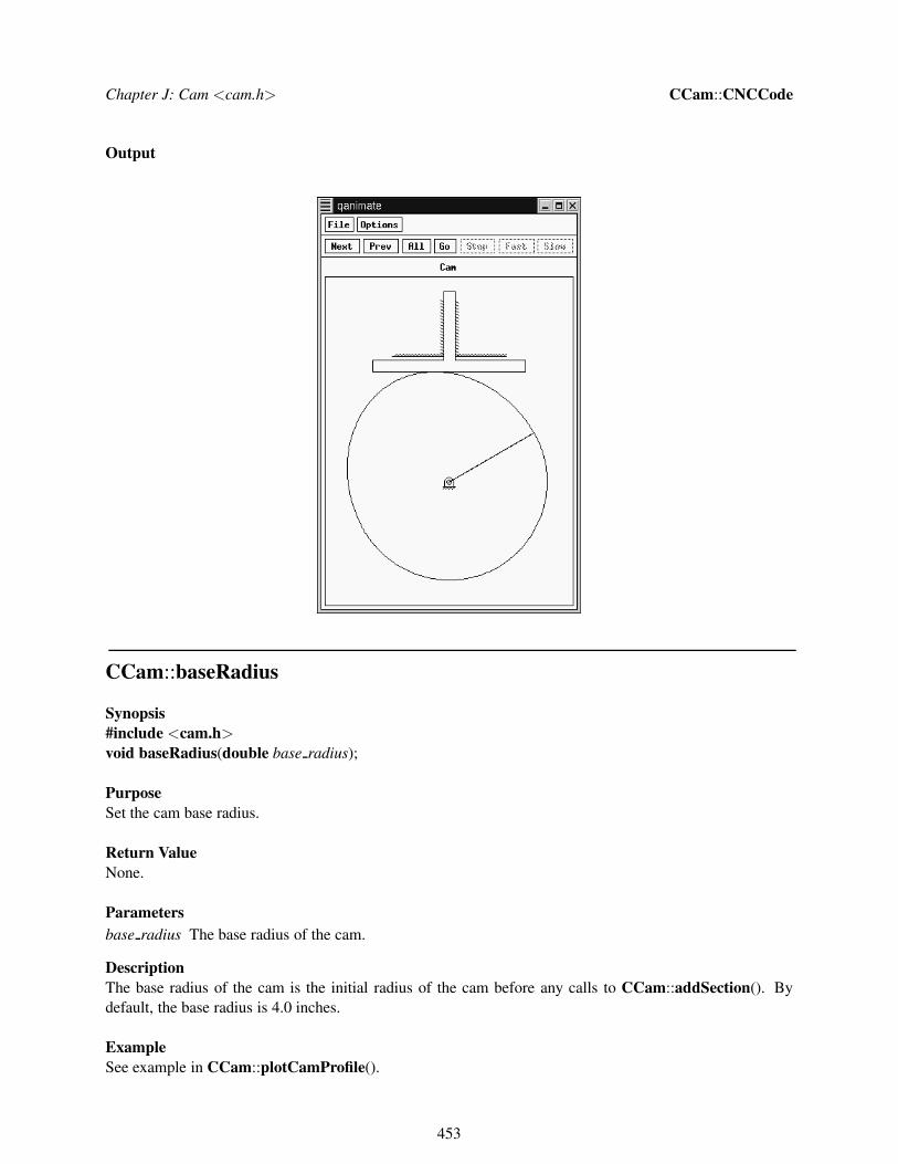
Chapter J: Cam <cam.h> CCam::CNCCode
Output
CCam::baseRadius
Synopsis
#include <cam.h>void baseRadius(double base radius);
Purpose
Set the cam base radius.
Return Value
None.
Parameters
base radius The base radius of the cam.
Description
The base radius of the cam is the initial radius of the cam before any calls to CCam::addSection(). By
default, the base radius is 4.0 inches.
Example
See example in CCam::plotCamProfile().
453

Chapter J: Cam <cam.h> CCam::cutDepth
See Also
CCam::addSection();
CCam::CNCCode
Synopsis
#include <cam.h>void CNCCode(string t filename);
Purpose
Set the filename for CNC code output.
Return Value
None.
Parameters
filename The name of the CNC code file to be created.
Description
This function sets the name of the CNC code file to be created. The file is created at the point when
CCam::makeCam() is called.
Example
#include <cam.h>
int main() {
class CCam cam;
int steps = 360;
cam.followerType(CAM_FOLLOWER_TRANS_FLAT, 0);
cam.cutter(.25, 2, 2);
cam.cutDepth(1.75);
cam.feedrate(10.5);
cam.spindleSpeed(2000);
cam.cutterOffset(1.0, 1.0, 0);
cam.addSection(90, .5, CAM_MOTION_HARMONIC);
cam.addSection(90, -.5, CAM_MOTION_HARMONIC);
cam.addSection(CAM_DURATION_FILL, 0, CAM_MOTION_HARMONIC);
cam.CNCCode("../output/CNCCode.txt");
cam.makeCam(steps);
}
Output
See Also
CCam::makeCam();
References
Vickers, G. W., Ly, M. H. and Oetter, R. G., 1990, Numerically Controlled Machine Tools, Ellis Horwood,
New York, NY.
454

Chapter J: Cam <cam.h> CCam::cutter
CCam::cutDepth
Synopsis
#include <cam.h>void cutDepth(double cut depth);
Purpose
Set the cut depth for CNC code generation.
Return Value
None.
Parameters
cut depth The depth of the cutter during cam manufacturing.
Description
This function sets the cutter depth to be used during cam manufacturing and is used during the creation of
the CNC code. This parameter does not effect the shape of the cam profile and only needs to be set if CNC
code will be generated. By default, the cut depth is 0.75 inch.
Example
See example in CCam::CNCCode().
See Also
CCam::CNCCode(), CCam::cutter(), CCam::cutterOffset(), CCam::feedrate(), and CCam::spindleSpeed().
CCam::cutter
Synopsis
#include <cam.h>void cutter(double cutter radius, double cutter length, int tool num);
Purpose
Set the cutter parameters for CNC code generation.
Return Value
None.
Parameters
cutter radius The radius (in inches) of the cutter used for manufacturing of the cam.
cutter length The length (in inches) of the cutter used for manufacturing the cam.
tool num The tool number of the cutter used.
Description
This function sets the parameters for the cutter used to generate CNC code. Figure 6.5 illustrates the cutter
parameters. The cutter length should be less than the depth set in CCam::cutDepth(). The CNC machine
to be used supports multiple tools, tool num can be used to specify the correct cutter. These parameters do
455

Chapter J: Cam <cam.h> CCam::deleteCam
not effect the shape of the cam profile and only need to be set if CNC code is to be created. By default the
cutter radius is 0.125 in., the cutter length is 1.0 in., and the tool number is 1.
Example
See example in CCam::CNCCode().
See Also
CCam::CNCCode(), CCam::cutDepth(), CCam::cutterOffset(), CCam::feedrate(), and CCam::spindleSpeed().
CCam::cutterOffset
Synopsis
#include <cam.h>void cutterOffset(double x offset, double y offset, double z offset);
Purpose
Set the cutter home position offset for CNC code generation.
Return Value
None.
Parameters
x offset The x coordinate of the cutter home position offset.
y offset The y coordinate of the cutter home position offset.
z offset The z coordinate of the cutter home position offset.
Description
The CNC home position offset may be changed if the CNC home position does not coincide with the de-
sired location of the cam center. As shown in Figure 6.6, the home position offset is measured from the old
home position to the new home position. It is important that these parameters be chosen properly, incorrect
selection can cause damage to the tools and CNC machine. These parameters do not effect the shape of the
cam profile and only need to be set if CNC code is to be created. By default, all offsets are zero.
Example
See example in CCam::CNCCode().
See Also
CCam::CNCCode(), CCam::cutDepth(), CCam::cutter(), CCam::feedrate(), and CCam::spindleSpeed().
CCam::deleteCam
Synopsis
#include <cam.h>void deleteCam();
456

Chapter J: Cam <cam.h> CCam::followerType
Purpose
Remove data from a previously used instance of the CCam class.
Return Value
None.
Parameters
None.
Description
This function frees all memory associated with previously allocated cam sections and data arrays. This
function allows for reuse of a single instance of the CCam class to create multiple cams.
CCam::feedrate
Synopsis
#include <cam.h>void feedrate(double feedrate);
Purpose
Set the feedrate for CNC code generation.
Return Value
None.
Parameters
feedrate The feedrate in inches per minute for machining.
Description
The feedrate, in inches per minute, is the rate at which the workpiece is moved during machining. This
parameter does not effect the shape of the cam profile and only needs to be set if CNC code is to be created.
By default, the feedrate is 18.3 in/min.
Example
See example in CCam::CNCCode().
See Also
CCam::CNCCode(), CCam::cutDepth(), CCam::cutter(), CCam::cutterOffset(), and CCam::spindleSpeed().
CCam::followerType
Synopsis
#include <cam.h>int followerType(int follower type, ... /* [double e], [double e, double rf], [double m, double f],
[double m, double A, double rf] */);
457

Chapter J: Cam <cam.h> CCam::followerType
Syntax
int followerType(CAM FOLLOWER TRANS FLAT, double e)
int followerType(CAM FOLLOWER TRANS ROLL, double e, double rf
int followerType(CAM FOLLOWER OSC FLAT, double m, double f)
int followerType(CAM FOLLOWER OSC ROLL, double m, double A, double rf)
Purpose
Set the cam follower type.
Return Value
This function returns 0 on success and -1 on failure.
Parameters
e For a translating follower, the distance from the cam center to the line of follower motion, as shown in
Figures 6.1 and 6.2. By default, e is zero.
rf The roller radius for a roller follower, as shown in Figures 6.2 and 6.4. By default, rf is 1.0 inch.
f For a flat-faced oscillating follower, the follower face offset measured from the follower pivot point, as
showin in Figure 6.3. By default, f is 4.0 inches.
A For an oscillating roller follower, the length of the arm connecting the pivot point and roller center, as
shown in Figure 6.4. By default, A is 10.0 inches.
m For oscillating followers, the distance between the cam center and the follower pivot point, as shown in
Figures 6.3 and 6.4. By default, m is 15.0 inches.
Description
This function is used to select the follower type and set the necessary related parameters. For a trans-
lating flat-faced follower, e is positive for an offset to the right of the cam. For a translating roller fol-
lower, e is positive for offsets to the left of the cam. For oscillating followers, m is positive when the
follower pivot point is to the right of the cam. All dimensions are in inches. By default, the follower type is
CAM FOLLOWER TRANS FLAT.
Example 1
#include <cam.h>
int main() {
class CCam cam;
int steps = 360;
CPlot plot;
cam.followerType(CAM_FOLLOWER_TRANS_FLAT, 0);
cam.baseRadius(5);
cam.addSection(90, .5, CAM_MOTION_HARMONIC);
cam.addSection(90, -.5, CAM_MOTION_HARMONIC);
cam.addSection(CAM_DURATION_FILL, 0, CAM_MOTION_HARMONIC);
cam.makeCam(steps);
cam.plotCamProfile(&plot);
}
458

Chapter J: Cam <cam.h> CCam::followerType
Output
-6
-5
-4
-3
-2
-1
0
1
2
3
4
5
6
-6 -5 -4 -3 -2 -1 0 1 2 3 4 5 6
y [in
]
x [in]
Cam Profile
Example 2
#include <cam.h>
int main() {
class CCam cam;
int steps = 360;
CPlot plot;
cam.followerType(CAM_FOLLOWER_TRANS_ROLL, .5, 1);
cam.baseRadius(5);
cam.addSection(90, .5, CAM_MOTION_HARMONIC);
cam.addSection(90, -.5, CAM_MOTION_HARMONIC);
cam.addSection(CAM_DURATION_FILL, 0, CAM_MOTION_HARMONIC);
cam.makeCam(steps);
cam.plotCamProfile(&plot);
}
Output
459

Chapter J: Cam <cam.h> CCam::followerType
-5
-4
-3
-2
-1
0
1
2
3
4
5
-5 -4 -3 -2 -1 0 1 2 3 4 5
y [in
]
x [in]
Cam Profile
Example 3
#include <cam.h>
int main() {
class CCam cam;
int steps = 360;
CPlot plot;
cam.followerType(CAM_FOLLOWER_OSC_FLAT, 10, 1);
cam.baseRadius(5);
cam.addSection(60, 3, CAM_MOTION_CYCLOIDAL);
cam.addSection(120, -3, CAM_MOTION_CYCLOIDAL);
cam.addSection(CAM_DURATION_FILL, 0, CAM_MOTION_HARMONIC);
cam.makeCam(steps);
cam.plotCamProfile(&plot);
}
Output
460

Chapter J: Cam <cam.h> CCam::followerType
-6
-5
-4
-3
-2
-1
0
1
2
3
4
5
6
-6 -5 -4 -3 -2 -1 0 1 2 3 4 5 6
y [in
]
x [in]
Cam Profile
Example 4
#include <cam.h>
int main() {
class CCam cam;
int steps = 360;
CPlot plot;
cam.followerType(CAM_FOLLOWER_OSC_ROLL, 10, 10, 1);
cam.baseRadius(5);
cam.addSection(60, 3, CAM_MOTION_CYCLOIDAL);
cam.addSection(120, -3, CAM_MOTION_CYCLOIDAL);
cam.addSection(CAM_DURATION_FILL, 0, CAM_MOTION_HARMONIC);
cam.makeCam(steps);
cam.plotCamProfile(&plot);
}
Output
461

Chapter J: Cam <cam.h> CCam::getCamAngle
-6
-5
-4
-3
-2
-1
0
1
2
3
4
5
6
-6 -5 -4 -3 -2 -1 0 1 2 3 4 5 6
y [in
]
x [in]
Cam Profile
CCam::getCamAngle
Synopsis
#include <cam.h>int getCamAngle(double angle[:]);
Purpose
Get the cam angular position data.
Return Value
This function returns 0 on success and -1 on failure.
Parameters
angle A double array of size steps+1 for the cam angular position data.
Description
This function copies an internal array containing the angular position of the cam into angle. The angle
array should be of size steps+1, where steps is the number of steps specified in CCam::makeCam(). This
function should only be called after CCam::makeCam().
Example
#include <cam.h>
int main() {
class CCam cam;
int steps = 360;
double angle[steps+1];
462

Chapter J: Cam <cam.h> CCam::getCamProfile
cam.followerType(CAM_FOLLOWER_TRANS_FLAT, 0);
cam.addSection(90, 1, CAM_MOTION_HARMONIC);
cam.addSection(90, -1, CAM_MOTION_HARMONIC);
cam.addSection(CAM_DURATION_FILL, 0, CAM_MOTION_HARMONIC);
cam.makeCam(steps);
cam.getCamAngle(angle);
}
See Also
CCam::getCamProfile(), CCam::getFollowerAccel(), CCam::getFollowerPos(), CCam::getFollowerVel,
CCam::getTransAngle(), CCam::makeCam().
CCam::getCamProfile
Synopsis
#include <cam.h>int getCamProfile(double x[:], double y[:]);
Purpose
Get the cam profile data.
Return Value
This function returns 0 on success and -1 on failure.
Parameters
x A double array of size steps+1 for the x coordinates of the cam profile.
y A double array of size steps+1 for the y coordinates of the cam profile.
Description
This function copies internal arrays containing the cam profile into x and y. The x and y arrays should be
of size steps+1, where steps is the number of steps specified in CCam::makeCam(). This function should
only be called after CCam::makeCam().
Example
#include <cam.h>
int main() {
class CCam cam;
class CPlot plot;
int steps = 360;
double x[steps+1], y[steps+1];
cam.followerType(CAM_FOLLOWER_TRANS_FLAT, 0);
cam.addSection(90, 1, CAM_MOTION_HARMONIC);
cam.addSection(90, -1, CAM_MOTION_HARMONIC);
cam.addSection(CAM_DURATION_FILL, 0, CAM_MOTION_HARMONIC);
cam.makeCam(steps);
cam.getCamProfile(x, y);
plotxy(x, y, "Cam Profile", "x", "y", &plot);
plot.sizeRatio(-1);
463

Chapter J: Cam <cam.h> CCam::getFollowerAccel
plot.plotting();
}
Output
-0.2
0
0.2
0.4
0.6
0.8
1
1.2
-0.4 -0.3 -0.2 -0.1 0 0.1 0.2 0.3 0.4
y
x
Cam Profile
See Also
CCam::makeCam().
CCam::getFollowerAccel
Synopsis
#include <cam.h>int getFollowerAccel(double accel[:]);
Purpose
Get the cam follower acceleration data.
Return Value
This function returns 0 on success and -1 on failure.
Parameters
accel A double array of size steps+1 for the cam acceleration data.
Description
This function copies an internal array containing the follower acceleration data into accel. The accel array
should be of size steps+1, where steps is the number of steps specified in CCam::makeCam(). This func-
tion should only be called after CCam::makeCam().
Example
#include <cam.h>
464

Chapter J: Cam <cam.h> CCam::getFollowerJerk
int main() {
class CCam cam;
class CPlot plot;
int steps = 360;
double angle[steps+1], accel[steps+1];
cam.followerType(CAM_FOLLOWER_TRANS_FLAT, 0);
cam.addSection(90, 1, CAM_MOTION_HARMONIC);
cam.addSection(90, -1, CAM_MOTION_HARMONIC);
cam.addSection(CAM_DURATION_FILL, 0, CAM_MOTION_HARMONIC);
cam.makeCam(steps);
cam.getCamAngle(angle);
cam.getFollowerAccel(accel);
plotxy(angle, accel, "Follower Acceleration", "Angle", "in/sˆ2", &plot);
plot.plotting();
}
Output
-2
-1.5
-1
-0.5
0
0.5
1
1.5
2
0 50 100 150 200 250 300 350 400
in/s
^2
Angle
Follower Acceleration
See Also
CCam::getCamAngle(), CCam::getCamProfile(), CCam::getFollowerPos(), CCam::getFollowerVel,
CCam::getFollowerJerk(), CCam::getTransAngle(), CCam::makeCam().
CCam::getFollowerJerk
Synopsis
#include <cam.h>int getFollowerJerk(double jerk[:]);
Purpose
Get the cam follower jerk data.
Return Value
465

Chapter J: Cam <cam.h> CCam::getFollowerPos
This function returns 0 on success and -1 on failure.
Parameters
jerk A double array of size steps+1 for the cam jerk data.
Description
This function copies an internal array containing the follower jerk data into jerk. The jerk array should be
of size steps+1, where steps is the number of steps specified in CCam::makeCam(). This function should
only be called after CCam::makeCam().
Example
#include <cam.h>
int main() {
class CCam cam;
class CPlot plot;
int steps = 360;
double angle[steps+1], jerk[steps+1];
cam.followerType(CAM_FOLLOWER_TRANS_FLAT, 0);
cam.addSection(90, 1, CAM_MOTION_HARMONIC);
cam.addSection(90, -1, CAM_MOTION_HARMONIC);
cam.addSection(CAM_DURATION_FILL, 0, CAM_MOTION_HARMONIC);
cam.makeCam(steps);
cam.getCamAngle(angle);
cam.getFollowerJerk(jerk);
plotxy(angle, jerk, "Follower Jerk", "Angle", "in/sˆ3", &plot);
plot.plotting();
}
Output
-4
-3
-2
-1
0
1
2
3
4
0 50 100 150 200 250 300 350 400
in/s
^3
Angle
Follower Jerk
See Also
CCam::getCamAngle(), CCam::getCamProfile(), CCam::getFollowerPos(), CCam::getFollowerVel,
466

Chapter J: Cam <cam.h> CCam::getFollowerPos
CCam::getFollowerAccel(), CCam::getTransAngle(), CCam::makeCam().
CCam::getFollowerPos
Synopsis
#include <cam.h>int getFollowerPos(double pos[:]);
Purpose
Get the cam follower position data.
Return Value
This function returns 0 on success and -1 on failure.
Parameters
pos A double array of size steps+1 for the follower position data.
Description
This function copies an internal array containing the follower position data into pos. The pos array should be
of size steps+1, where steps is the number of steps specified in CCam::makeCam(). This function should
only be called after CCam::makeCam().
Example
#include <cam.h>
int main() {
class CCam cam;
class CPlot plot;
int steps = 360;
double angle[steps+1], pos[steps+1];
cam.followerType(CAM_FOLLOWER_TRANS_FLAT, 0);
cam.addSection(90, 1, CAM_MOTION_HARMONIC);
cam.addSection(90, -1, CAM_MOTION_HARMONIC);
cam.addSection(CAM_DURATION_FILL, 0, CAM_MOTION_HARMONIC);
cam.makeCam(steps);
cam.getCamAngle(angle);
cam.getFollowerPos(pos);
plotxy(angle, pos, "Follower Position", "Angle", "in", &plot);
plot.sizeRatio(-1);
plot.plotting();
}
Output
467

Chapter J: Cam <cam.h> CCam::getFollowerVel
4
4.2
4.4
4.6
4.8
5
0 50 100 150 200 250 300 350 400
in
Angle
Follower Position
See Also
CCam::getCamAngle(), CCam::getCamProfile(), CCam::getFollowerAccel(), getFollowerVel(),
CCam::getTransAngle(), CCam::makeCam().
CCam::getFollowerVel
Synopsis
#include <cam.h>int getFollowerVel(double vel[:]);
Purpose
Get the cam follower velocity data.
Return Value
This function returns 0 on success and -1 on failure.
Parameters
vel A double array of size steps+1 for the follower velocity data.
Description
This function copies an internal array containing the follower velocity data into vel. The vel array should be
of size steps+1, where steps is the number of steps specified in CCam::makeCam(). This function should
only be called after CCam::makeCam().
Example
#include <cam.h>
int main() {
class CCam cam;
class CPlot plot;
int steps = 360;
468

Chapter J: Cam <cam.h> CCam::makeCam
double angle[steps+1], vel[steps+1];
cam.followerType(CAM_FOLLOWER_TRANS_FLAT, 0);
cam.addSection(90, 1, CAM_MOTION_HARMONIC);
cam.addSection(90, -1, CAM_MOTION_HARMONIC);
cam.addSection(CAM_DURATION_FILL, 0, CAM_MOTION_HARMONIC);
cam.makeCam(steps);
cam.getCamAngle(angle);
cam.getFollowerVel(vel);
plotxy(angle, vel, "Follower Velocity", "Angle", "in", &plot);
plot.sizeRatio(-1);
plot.plotting();
}
Output
-1
-0.5
0
0.5
1
0 50 100 150 200 250 300 350 400
in
Angle
Follower Velocity
See Also
CCam::getCamAngle(), CCam::getCamProfile(), CCam::getFollowerAccel(), CCam::getFollowerPos(),
CCam::getTransAngle(), CCam::makeCam().
CCam::makeCam
Synopsis
#include <cam.h>int makeCam(int steps)
Purpose
Generate the cam data and write CNC code to a file.
Return Value
This function returns 0 on success and -1 on failure.
Parameters
469

Chapter J: Cam <cam.h> CCam::makeCam
steps The number of steps used in calculating the cam profile and other results.
Description
This function is called to perform the actual calculations necessary to generate the results. It should be called
after all other member functions have been called except for CCam::animation(), CCam::getCamAngle(),
CCam::getCamProfile(), CCam::getFollowerAccel(), CCam::getFollowerPos(), CCam::getFollowerVel(),
CCam::getTransAngle(), CCam::plotCamProfile(), CCam::plotFollowerAccel(), CCam::plotFollowerPos(),
CCam::plotFollowerVel(), and CCam::plotTransAngle(). The cam is divided into steps segments, giving
steps+1 data points for the range of cam positions between 0 and 360 deg., inclusive. The results are
stored in internal arrays for later plotting or access by the user. If a CNC file name was specified using
CCam::CNCCode(), CNC code is written to the specified file.
Algorithm
When the CCam class is ready to calculate the cam profile, a loop is started. The variable φ starts at 0◦ and
each time through the loop it is increased by 360◦/steps. The loop ends just before φ exceeds the number of
degrees specified by the duration for the section.
Each time through the loop (for each value of phi), the position, velocity, and acceleration of the follower is
calculated based on the type of motion specified by the user (harmonic or cycloidal). This loop is repeated
for each section of the cam. The equations used in the calculations are shown below where L is the Lift over
the duration of the section (in inches for a translating follower and radians for an oscillating follower), β is
the section duration (in radians) and φ is the cam position relative to the beginning of the section (in radians).
The equations for harmonic motion are: (Erdman and Sandor, pp. 371-2)
y =L
2
[
1− cos
(
πφ
β
)]
v =πL
2βω sin
(
πφ
β
)
a =π2L
2β2ω2 cos
(
πφ
β
)
jerk =π3L
2β3ω3 sin
(
πφ
β
)
The equations for cycloidal motion are: (Erdman and Sandor, pp. 372-3)
y = L
[
φ
β−
1
2πsin
(
2πφ
β
)]
v =L
βω
[
1− cos
(
2πφ
β
)]
a =2πL
β2ω2 sin
(
2πφ
β
)
jerk =4π2L
β3ω3 cos
(
2πφ
β
)
For translating followers the above equations produce the linear position, velocity and acceleration of the
follower. For oscillating followers, the equations produce the angular position, angular velocity and angular
470

Chapter J: Cam <cam.h> CCam::makeCam
acceleration of the follower. Once the position, velocity, and acceleration are calculated for a given value of
φ, the coordinates of the cam profile and cutter center are calculated.
For a translating flat-faced follower, the angle between the direction of follower translation and the contact
point of the cam and follower is: (Erdman and Sandor, pp. 392)
θ = arctan
(
1
L
dL
dφ
)
= arctan
(
v
Lω
)
The distance between the cam center and the point of contact is:
R =L
cos θ
The coordinates of the cam profile with respect to the reference radial is:
xcam = R cos (φtotal + θ)
ycam = R sin (φtotal + θ)
The angle between the direction of follower translation and the center of the cutter is:
γ = arctan
(
R sin θ
L+ rc
)
The distance between the cam center and cutter center is:
c =L+ rccos γ
The coordinates of the cutter center with respect to the reference radial is:
xcutter = c cos (γ + φtotal)
ycutter = c sin (γ + φtotal)
For an oscillating flat-faced follower, the angel between the normal to the follower face and the point of
contact is: (Erdman and Sandor, pp. 394)
θ = arctan
[(
(dζ/dφ)
1− (dζ/dφ)
)
m cos ζ
f −m sin ζ
]
= arctan
[(
(v/ω)
(1− v/ω)
)
m cos ζ
f −m sin ζ
]
The distance between the cam center and the contact point is:
471

Chapter J: Cam <cam.h> CCam::makeCam
R =f +m sin ζ
cos θ
The coordinates of the cam profile with respect to the reference radial is:
xcam = R cos
(
φtotal + θ +π
2+ ζ
)
ycam = R sin
(
φtotal + θ +π
2+ ζ
)
The coordinates of the cutter center with respect to the reference radial is:
xcutter =√
c2x + c2y cos
(
φtotal + θ +π
2+ ζ − arctan
cxcy
)
ycutter =√
c2x + c2y sin
(
φtotal + θ +π
2+ ζ − arctan
cxcy
)
where
cx = R+ rc cos θ
cy = rc sin θ
For a translating roller follower the angle between the contact point of the cam and follower and the cam
center is:
α = arctan
[
L(dL/dφ)
m2 + L2 −m(dL/dφ)
]
= arctan
[
L(v/ω)
m2 + L2 −m(v/ω)
]
The pressure angle is:
δ = α− ψ
where
ψ = arctan(m
L)
The distance between the cam and follower centers is
F =√
L2 +m2
The coordinates of the cam profile with respect to the reference radial are:
472

Chapter J: Cam <cam.h> CCam::makeCam
xcam =√
Rx2 +Ry
2 cos(φtotal + ψ + arctan(Ry/Rx)
ycam =√
Rx2 +Ry
2 sin(φtotal + ψ + arctan(Ry/Rx)
where
Rx = F − rf cosα
Ry = rf sinα
The coordinates of the cutter location with respect to the reference radial are:
xcutter =√
c2x + c2y cos(φtotal + ψ + arctan(cy/cx)
ycutter =√
c2x + c2y sin(φtotal + ψ + arctan(cy/cx)
where
cx = F + (rc − rf ) cosα
cy = (rf − rc) sinα
For an oscillating roller follower, angle between the follower center and the cam/follower contact point is
α = arctan
[
(A sin γ) (dζ/dφ)
L− (A cos γ) (dζ/dφ)
]
= arctan
[
(A sin γ) (v/ω)
L− (A cos γ) (v/ω)
]
where
L = (A2 +m2 − 2Am cos(ζ))
γ = arcsin(m sin(ζ)/L)
The initial follower angle is
ζ0 = cos−1((A2 +m2 − (rb + rf )2)/(2mA)
The pressure angle is
δ = γ + α+−π
2
The coordinates of the cam profile with respect to the reference radial are:
473

Chapter J: Cam <cam.h> CCam::plotCamProfile
xcam =√
R2x +R2
y cos[φtotal + π − γ − ζ + arctan(Ry
Rx)]
ycam =√
R2x +R2
y sin[φtotal + π − γ − ζ + arctan(Ry
Rx)]
where
Rx = L− rf cosα
Ry = rf sinα
The coordinates of the cutter center with respect to the reference radial are:
xcutter =√
c2x + c2y cos[φtotal + π − γ − ζ + arctan(cycx
)]
ycutter =√
c2x + c2y sin[φtotal + π − γ − ζ + arctan(cycx
)]
cx = L+ (rc − rf ) cosα
cy = (rf − rc) sinα
References
Erdman, A. G. and Sandor, G. N., 1997, Mechanism Design Analysis and Synthesis, Vol. 1, 3rd ed., Prentice
Hall, Englewood Cliffs, NJ.
CCam::plotCamProfile
Synopsis
#include <cam.h>int plotCamProfile(CPlot *plot);
Syntax
plotCamProfile(&plot)
Purpose
Plot the cam profile data.
Return Value
This function returns 0 on success and -1 on failure.
Parameters
&plot A pointer to a CPlot class variable for formatting the plot of the cam profile.
Description
Plot the cam profile. This function should only be called after CCam::makeCam().
Example
474

Chapter J: Cam <cam.h> CCam::plotFollowerAccel
#include <cam.h>
int main() {
class CCam cam;
class CPlot plot;
int steps = 360;
cam.followerType(CAM_FOLLOWER_TRANS_FLAT, 0);
cam.baseRadius(5);
cam.addSection(90, 1, CAM_MOTION_HARMONIC);
cam.addSection(90, -1, CAM_MOTION_HARMONIC);
cam.addSection(CAM_DURATION_FILL, 0, CAM_MOTION_HARMONIC);
cam.makeCam(steps);
cam.plotCamProfile(&plot);
}
Output
-7
-6
-5
-4
-3
-2
-1
0
1
2
3
4
5
6
7
-7 -6 -5 -4 -3 -2 -1 0 1 2 3 4 5 6 7
y [in
]
x [in]
Cam Profile
See Also
CCam::makeCam().
CCam::plotFollowerAccel
Synopsis
#include <cam.h>int plotFollowerAccel(CPlot *plot);
Syntax
plotFollowerAccel(&plot)
Purpose
Plot the cam follower acceleration vs. the cam angular position.
475

Chapter J: Cam <cam.h> CCam::plotFollowerJerk
Return Value
This function returns 0 on success and -1 on failure.
Parameters
&plot A pointer to a CPlot class variable for formatting the plot of the cam follower acceleration.
Description
Plot the cam follower acceleration. This function should only be called after CCam::makeCam().
Example
#include <cam.h>
int main() {
class CCam cam;
class CPlot plot;
int steps = 360;
cam.followerType(CAM_FOLLOWER_TRANS_FLAT, 0);
cam.baseRadius(5);
cam.addSection(90, 1, CAM_MOTION_HARMONIC);
cam.addSection(90, -1, CAM_MOTION_HARMONIC);
cam.addSection(CAM_DURATION_FILL, 0, CAM_MOTION_HARMONIC);
cam.makeCam(steps);
cam.plotFollowerAccel(&plot);
}
Output
-2
-1.5
-1
-0.5
0
0.5
1
1.5
2
0 50 100 150 200 250 300 350
acce
lera
tion
[in/s
^2]
theta [deg]
Acceleration vs. Theta
See Also
CCam::makeCam().
CCam::plotFollowerJerk
476

Chapter J: Cam <cam.h> CCam::plotFollowerJerk
Synopsis
#include <cam.h>int plotFollowerJerk(CPlot *plot);
Syntax
plotFollowerJerk(&plot)
Purpose
Plot the cam follower jerk vs. the cam angular position.
Return Value
This function returns 0 on success and -1 on failure.
Parameters
&plot A pointer to a CPlot class variable for formatting the plot of the cam follower jerk.
Description
Plot the cam follower jerk. This function should only be called after CCam::makeCam().
Example
#include <cam.h>
int main() {
class CCam cam;
class CPlot plot;
int steps = 360;
cam.followerType(CAM_FOLLOWER_TRANS_FLAT, 0);
cam.baseRadius(5);
cam.addSection(90, 1, CAM_MOTION_HARMONIC);
cam.addSection(90, -1, CAM_MOTION_HARMONIC);
cam.addSection(CAM_DURATION_FILL, 0, CAM_MOTION_HARMONIC);
cam.makeCam(steps);
cam.plotFollowerJerk(&plot);
}
Output
477

Chapter J: Cam <cam.h> CCam::plotFollowerPos
-4
-3
-2
-1
0
1
2
3
4
0 50 100 150 200 250 300 350
jerk
[m/s
^3]
theta [deg]
Jerk vs. Theta
See Also
CCam::makeCam().
CCam::plotFollowerPos
Synopsis
#include <cam.h>int plotFollowerPos(CPlot *plot);
Syntax
plotFollowerPos(&plot)
Purpose
Plot the cam follower position vs. the cam angular position.
Return Value
This function returns 0 on success and -1 on failure.
Parameters
&plot A pointer to a CPlot class variable for formatting the plot of the cam follower position.
Description
Plot the cam follower position. This function should only be called after CCam::makeCam().
Example
#include <cam.h>
int main() {
class CCam cam;
class CPlot plot;
int steps = 360;
cam.followerType(CAM_FOLLOWER_TRANS_FLAT, 0);
478

Chapter J: Cam <cam.h> CCam::plotFollowerVel
cam.baseRadius(5);
cam.addSection(90, 1, CAM_MOTION_HARMONIC);
cam.addSection(90, -1, CAM_MOTION_HARMONIC);
cam.addSection(CAM_DURATION_FILL, 0, CAM_MOTION_HARMONIC);
cam.makeCam(steps);
cam.plotFollowerPos(&plot);
}
Output
5
5.2
5.4
5.6
5.8
6
0 50 100 150 200 250 300 350
posi
tion
[in]
theta [deg]
Position vs. Theta
See Also
CCam::makeCam().
CCam::plotFollowerVel
Synopsis
#include <cam.h>int plotFollowerVel(CPlot *plot);
Syntax
plotFollowerVel(&plot)
Purpose
Plot the cam follower velocity vs. the cam angular position.
Return Value
This function returns 0 on success and -1 on failure.
Parameters&plot A pointer to a CPlot class variable for formatting the plot of the cam follower velocity.
Description
Plot the cam follower velocity. This function should only be called after CCam::makeCam().
479

Chapter J: Cam <cam.h> CCam::plotTransAngle
Example
#include <cam.h>
int main() {
class CCam cam;
class CPlot plot;
int steps = 360;
cam.followerType(CAM_FOLLOWER_TRANS_FLAT, 0);
cam.baseRadius(5);
cam.addSection(90, 1, CAM_MOTION_HARMONIC);
cam.addSection(90, -1, CAM_MOTION_HARMONIC);
cam.addSection(CAM_DURATION_FILL, 0, CAM_MOTION_HARMONIC);
cam.makeCam(steps);
cam.plotFollowerVel(&plot);
}
Output
-1
-0.5
0
0.5
1
0 50 100 150 200 250 300 350
velo
city
[in/
s]
theta [deg]
Vel vs. Theta
See Also
CCam::makeCam().
CCam::plotTransAngle
Synopsis
#include <cam.h>int plotTransAngle(CPlot *plot);
Syntax
plotTransAngle(&plot)
Purpose
Plot the cam transmission angle vs. the cam angular position.
480

Chapter J: Cam <cam.h> CCam::spindleSpeed
Return Value
This function returns 0 on success and -1 on failure.
Parameters
&plot A pointer to a CPlot class variable for formatting the plot of the cam transmission angle.
Description
Plot the cam transmission angle. This function should only be called after CCam::makeCam().
Example
#include <cam.h>
int main() {
class CCam cam;
class CPlot plot;
int steps = 360;
cam.followerType(CAM_FOLLOWER_TRANS_FLAT, 0);
cam.baseRadius(5);
cam.addSection(90, 1, CAM_MOTION_HARMONIC);
cam.addSection(90, -1, CAM_MOTION_HARMONIC);
cam.addSection(CAM_DURATION_FILL, 0, CAM_MOTION_HARMONIC);
cam.makeCam(steps);
cam.plotTransAngle(&plot);
}
Output
78
80
82
84
86
88
90
0 50 100 150 200 250 300 350
Tra
nsm
issi
on A
ngle
[deg
]
theta [deg]
Transmission Angle vs. Theta
See Also
CCam::makeCam().
CCam::spindleSpeed
481

Chapter J: Cam <cam.h> CCam::spindleSpeed
Synopsis
#include <cam.h>void spindleSpeed(double spindle speed);
Purpose
Set the spindle speed for CNC code generation.
Return Value
None.
Parameters
spindle speed The spindle speed for the cutter in RPM (revolution per minute).
Description
The spindle speed is the rotational speed of the cutter in RPM. This parameter does not effect the shape of
the cam profile and only needs to be set if CNC code is to be created. By default, the spindle speed is 3036
RPM.
Example
See example in CCam::CNCCode().
See Also
CCam::CNCCode(), CCam::cutDepth(), CCam::cutter(), CCam::cutterOffset(), and CCam::feedrate().
482

Chapter J: Cam <cam.h> cam.ch
cam.ch
Synopsis
cam.ch [-acceleration]
[-animate]
[-base radius]
[-cncfile filename]
[-cutter radius length num]
[-depth depth]
[-feedrate rate]
[-follower follower type [e] [e rf] [m f] [m A rf]]
[-offset x y z]
[-omega omega]
[-output display]
[-position]
[-profile]
-steps num
[-section duration displacement motion type]
[-spindle speed]
[-transangle]
[-velocity]
Syntax
As many of the optional arguments as desired can be used. The minimum number of arguments required
to produce meaningful results are steps, two sections, and at least one of the output options (-acceleration,
-animate, -position, -profile, -transangle, -velocity).
Purpose
This program provides a command line interface to the design capabilities of the CCam class.
Return Value
This program returns 0 on successful completion, or -1 if there is an error.
Arguments
steps The number of steps used in calculating the cam. See CCam::makeCam().
acceleration Plot the follower acceleration. See CCam::plotFollowerAccel().
animate Animate the cam using xlinkage. See CCam::animation().
base The base radius of the cam. See CCam::baseRadius.
cncfile The name of a file for CNC code output. See CCam::CNCCode().
cutter The cutter parameters for CNC code generation. See CCam::cutter().
depth The cutter depth for CNC code generation. See CCam::cutDepth().
feedrate The feedrate for CNC code generation. See CCam::feedrate.
483

Chapter J: Cam <cam.h> cam.ch
follower The follower type and related parameters. See CCam::followerType().
offset The cutter home position offset CNC code generation. See CCam::cutterOffset().
omega The angular velocity of the cam. See CCam::angularVel().
output The output type for plots and animation. This can be CAM OUTPUT DISPLAYor CAM OUTPUT STREAM.
File output is not supported.
position Plot the follower position. See CCam::plotFollowerPos().
profile Plot the cam profile. See CCam::plotCamProfile().
section The parameters for a new cam section. See CCam::addSection().
spindle The cutter spindle speed for CNC code generation. See CCam::spindleSpeed().
transangle Plot the transmission angle. See CCam::plotTransAngle().
velocity Plot the follower velocity. See CCam::plotFollowerVel().
Description
The program functions as a command line interface to the design capabilities of the CCam class. It was
developed primarily for use internally by the Web-based cam design tools.
Example 1
cam.ch -section 90 .75 CAM_MOTION_HARMONIC -section 90 -.75
CAM_MOTION_HARMONIC -section CAM_DURATION_FILL 0 CAM_MOTION_HARMONIC
-steps 300 -profile -animate 30
Output
484

Chapter J: Cam <cam.h> cam.ch
Example 2
cam.ch -section 60 .5 CAM_MOTION_CYCLOIDAL -section 30 0
CAM_MOTION_CYCLOIDAL -section 210 -.5 CAM_MOTION_CYCLOIDAL -section
CAM_DURATION_FILL 0 CAM_MOTION_HARMONIC -follower CAM_FOLLOWER_TRANS_ROLL
1 1.5 -base 4.5 -steps 500 -position
Output
485

Chapter J: Cam <cam.h> cam.ch
See Also
CCam class.
486

Index
addSection, 448, see CCam
angularAccel, see CFourbar, see CCrankSlider, see
CGearedFivebar, see CFourbarSlider, see CWattSixbarI,
see CWattSixbarII, see CStevSixbarI, see CStevSixbarIII
angularAccels, see CFourbar
angularPos, see CFourbar, see CCrankSlider, see CGeared-
Fivebar, see CFourbarSlider, see CWattSixbarI,
see CWattSixbarII, see CStevSixbarI, see CStevSixbarIII
angularPoss, see CFourbar
angularVel, see CFourbar, see CCrankSlider, see CGeared-
Fivebar, see CFourbarSlider, see CWattSixbarI,
see CWattSixbarII, see CStevSixbarI, see CStevSixbarIII,
448, see CCam
angularVels, see CFourbar
animation, 2, see CFourbar, see CCrankSlider, see
CGearedFivebar, see CFourbarSlider, see CWattSixbarI,
see CWattSixbarII, see CStevSixbarI, see CStevSixbarIII,
448, see CCam
baseRadius, 448, see CCam
C/C++, 2
cam.ch, 483
CAM DURATION FILL, 449, 450
CAM FOLLOWER OSC FLAT, 449
CAM FOLLOWER OSC ROLL, 449
CAM FOLLOWER TRANS FLAT, 449
CAM FOLLOWER TRANS ROLL, 449
CAM MOTION CYCLOIDAL, 449, 450
CAM MOTION HARMONIC, 449, 450
CCam, 448, 448
˜CCam, 448
addSection, 448, 450
angularVel, 448, 450
animation, 448, 452
baseRadius, 448, 453
CCam, 448
CNCCode, 448, 454
cutDepth, 448, 455
cutter, 448, 455
cutterOffset, 448, 456
deleteCam, 448, 456
feedrate, 448, 457
followerType, 448, 457
getCamAngle, 448, 462
getCamProfile, 448, 463
getFollowerAccel, 449, 464
getFollowerJerk, 449, 465
getFollowerPos, 449, 467
getFollowerVel, 449, 468
getTransAngle, 449
makeCam, 449, 469
plotCamProfile, 449, 474
plotFollowerAccel, 449, 475
plotFollowerJerk, 449, 476
plotFollowerPos, 449, 478
plotFollowerVel, 449, 479
plotTransAngle, 449, 480
spindleSpeed, 449, 481
CCrankSlider, 293
angularAccel, 294
angularPos, 296
angularVel, 297
animation, 298
couplerCurve, 299
couplerPointAccel, 301
couplerPointPos, 302
couplerPointVel, 303
displayPosition, 304
forceTorque, 305
forceTorques, 307
getJointLimits, 310
plotCouplerCurve, 311
plotForceTorques, 312
setAngularVel, 315
setCouplerPoint, 314
setGravityCenter, 314
setInertia, 315
setLinks, 316
setMass, 316
487

Chapter J: Cam <cam.h>
setNumPoints, 317
sliderAccel, 317
sliderPos, 319
sliderVel, 320
transAngle, 321
uscUnit, 322
CFourbar, 239
angularAccel, 241
angularAccels, 243
angularPos, 244
angularPoss, 245
angularVel, 247
angularVels, 248
animation, 250
couplerCurve, 258
couplerPointAccel, 261
couplerPointPos, 262
couplerPointVel, 263, 357
displayPosition, 265
displayPositions, 267
forceTorque, 267
forceTorques, 269
getAngle, 272
getJointLimits, 272
grashof, 274
plotAngularAccels, 275
plotAngularPoss, 276
plotAngularVels, 278
plotCouplerCurve, 279
plotForceTorques, 280
plotTransAngles, 281
printJointLimits, 282
setAngularVel, 283
setCouplerPoint, 284
setGravityCenter, 285
setInertia, 285
setLinks, 286
setMass, 286
setNumPoints, 287
synthesis, 287
transAngle, 289
transAngles, 290
uscUnit, 291
CFourbarSlider, 344
angularAccel, 345
angularPos, 347
angularVel, 349
animation, 351
couplerPointAccel, 353
couplerPointPos, 355
displayPosition, 359
setAngularVel, 361
setCouplerPoint, 360
setLinks, 362
setNumPoints, 362
sliderAccel, 363
sliderPos, 364
sliderVel, 366
uscUnit, 368
CGearedFivebar, 323
angularAccel, 324
angularPos, 326
angularVel, 328
animation, 329
couplerCurve, 331
couplerPointAccel, 333
couplerPointPos, 335
couplerPointVel, 336
displayPosition, 337
plotCouplerCurve, 339
setAngularVel, 342
setCouplerPoint, 341
setLinks, 342
setNumPoints, 343
uscUnit, 343
CGI, 223
CGI Programming, 219
CNCCode, 448, see CCam
complexsolvePP(), 7
complexsolvePR(), 6
complexsolveRP(), 8
complexsolveRR(), 6
complexsolveRRz(), 9
copyright, ii
COUPLER LINK3, 238
COUPLER LINK4, 238
COUPLER LINK5, 238
COUPLER LINK6, 238
COUPLER LINK7, 238
couplerCurve, see CFourbar, see CCrankSlider, see
CGearedFivebar
couplerPointAccel, see CFourbar, see CCrankSlider,
see CGearedFivebar, see CFourbarSlider, see
CWattSixbarI, see CWattSixbarII, see CStevSixbarI,
see CStevSixbarIII
488

Chapter J: Cam <cam.h>
couplerPointPos, see CFourbar, see CCrankSlider, see
CGearedFivebar, see CFourbarSlider, see CWattSixbarI,
see CWattSixbarII, see CStevSixbarI, see CStevSixbarIII
couplerPointVel, see CFourbar, see CCrankSlider, see
CGearedFivebar, see CFourbarSlider, see CWattSixbarI,
see CWattSixbarII, see CStevSixbarI, see CStevSixbarIII
CStevSixbarI, 408
angularAccel, 409
angularPos, 411
angularVel, 413
animation, 415
couplerPointAccel, 417
couplerPointPos, 419
couplerPointVel, 421
displayPosition, 423
setAngularVel, 426
setCouplerPoint, 425
setLinks, 426
setNumPoints, 427
uscUnit, 427
CStevSixbarIII, 429
angularAccel, 430
angularPos, 432
angularVel, 433
animation, 435
couplerPointAccel, 437
couplerPointPos, 439
couplerPointVel, 440
displayPosition, 442
setAngularVel, 445
setCouplerPoint, 444
setLinks, 445
setNumPoints, 446
uscUnit, 446
cutDepth, 448, see CCam
cutter, 448, see CCam
cutterOffset, 448, see CCam
CWattSixbarI, 369
angularAccel, 370
angularPos, 372
angularVel, 373
animation, 375
couplerPointAccel, 377
couplerPointPos, 379
couplerPointVel, 381
displayPosition, 383
setAngularVel, 386
setCouplerPoint, 385
setLinks, 386
setNumPoints, 387
uscUnit, 387
CWattSixbarII, 388
angularAccel, 389
angularPos, 391
angularVel, 393
animation, 395
couplerPointAccel, 398
couplerPointPos, 400
couplerPointVel, 401
displayPosition, 401
getIORanges, 403
setAngularVel, 405
setCouplerPoint, 404
setLinks, 405
setNumPoints, 406
uscUnit, 406
deleteCam, 448, see CCam
displayPosition, see CFourbar, see CCrankSlider, see
CGearedFivebar, see CFourbarSlider, see CWattSixbarI,
see CWattSixbarII, see CStevSixbarI, see CStevSixbarIII
displayPositions, see CFourbar
embeddable, 2
features, 1
feedrate, 448, see CCam
followerType, 448, see CCam
forceTorque, see CFourbar, see CCrankSlider
forceTorques, see CFourbar, see CCrankSlider
FOURBAR CRANKCRANK, 241
FOURBAR CRANKROCKER, 240
FOURBAR INVALID, 240
FOURBAR INWARDINWARD, 241
FOURBAR INWARDOUTWARD, 241
FOURBAR LINK1, 240
FOURBAR LINK2, 240
FOURBAR LINK3, 240
FOURBAR LINK4, 240
FOURBAR OUTWARDINWARD, 241
FOURBAR OUTWARDOUTWARD, 241
FOURBAR ROCKERCRANK, 241
FOURBAR ROCKERROCKER, 241
getAngle, see CFourbar
getCamAngle, 448, see CCam
getCamProfile, 448, see CCam
489

Chapter J: Cam <cam.h>
getFollowerAccel, 449, see CCam
getFollowerJerk, 449, see CCam
getFollowerPos, 449, see CCam
getFollowerVel, 449, see CCam
getIORanges, see CWattSixbarII
getJointLimits, see CFourbar, see CCrankSlider
getTransAngle, 449
grashof, see CFourbar
HTML, 220
tags, 223
linkage, 9, 237
M DEG2RAD(), 237
M FT2M, 237
M LB2N, 237
M LBFT2NM, 237
M LBFTSS2KGMM, 237
M RAD2DEG(), 237
M SLUG2KG, 237
makeCam, 449, see CCam
object-oriented, 2
plotAngularAccels, see CFourbar
plotAngularPoss, see CFourbar
plotAngularVels, see CFourbar
plotCamProfile, 449, see CCam
plotCouplerCurve, see CFourbar, see CCrankSlider,
see CGearedFivebar
plotFollowerAccel, 449, see CCam
plotFollowerJerk, 449, see CCam
plotFollowerPos, 449, see CCam
plotFollowerVel, 449, see CCam
plotForceTorques, see CFourbar, see CCrankSlider
plotting, 2
plotTransAngle, 449, see CCam
plotTransAngles, see CFourbar
printJointLimits, see CFourbar
qanimate, 196
QANIMATE OUTPUTTYPE DISPLAY, 237
QANIMATE OUTPUTTYPE FILE, 238
QANIMATE OUTPUTTYPE STREAM, 238
setAngularVel, see CFourbar, see CCrankSlider, see
CGearedFivebar, see CFourbarSlider, see CWattSixbarI,
see CWattSixbarII, see CStevSixbarI, see CStevSixbarIII
setCouplerPoint, see CFourbar, see CCrankSlider, see
CGearedFivebar, see CFourbarSlider, see CWattSixbarI,
see CWattSixbarII, see CStevSixbarI, see CStevSixbarIII
setGravityCenter, see CFourbar, see CCrankSlider
setInertia, see CFourbar, see CCrankSlider
setLinks, see CFourbar, see CCrankSlider, see CGeared-
Fivebar, see CFourbarSlider, see CWattSixbarI,
see CWattSixbarII, see CStevSixbarI, see CStevSixbarIII
setMass, see CFourbar, see CCrankSlider
setNumPoints, see CFourbar, see CCrankSlider, see
CGearedFivebar, see CFourbarSlider, see CWattSixbarI,
see CWattSixbarII, see CStevSixbarI, see CStevSixbarIII
sliderAccel, see CCrankSlider
seeCFourbarSlider, 363
sliderPos, see CCrankSlider
seeCFourbarSlider, 364
sliderVel, see CCrankSlider
seeCFourbarSlider, 366
spindleSpeed, 449, see CCam
synthesis, see CFourbar
transAngle, see CFourbar, see CCrankSlider
transAngles, see CFourbar
unwrap(), 16
uscUnit, see CFourbar, see CCrankSlider, see CGeared-
Fivebar, see CFourbarSlider, see CWattSixbarI,
see CWattSixbarII, see CStevSixbarI, see CStevSixbarIII
490