Ch 7: Loglinear Models

I Logistic regression and other models in Ch 3–6, 8–10 distinguishbetween a response variable Y and explanatory vars x1, x2, etc.

I Loglinear models for contingency tables treat all variables asresponse variables, like multivariate analysis.

Ex. Survey of high school seniors (see text):

IY1: used alchohol? (yes, no)

IY2: cigarettes? (yes, no)

IY3: marijuana? (yes, no)

Interested in patterns of dependence and independence among thethree variables:

I Any variables independent?I Strength of associations?I Interactions?

400

I Loglinear models treat cell counts as Poisson and use log link fcn.

Motivation: In I⇥ J table, X and Y are independent if

Pr(X = i, Y = j) = Pr(X = i)Pr(Y = j) for all i, ji.e., ⇡

ij

= ⇡

i+⇡+j

For expected cell frequencies,

µ

ij

= n⇡

ij

(general form)= n⇡

i+⇡+j

(under independence)

=) log(µij

) = �+ �

X

i

+ �

Y

j

�

X

i

: effect of classification in row i (I- 1 nonredundant parameters)

�

Y

j

: effect of classification in col j (J- 1 nonredundant parameters)

Loglinear model of independence: treats X and Y symmetrically.Unlike, e.g., logistic regr where Y = response, X = explanatory.

401

Note: For a Poisson loglinear model,

df = number of Poisson counts - number of parameters

Here number of Poisson counts = number cells in table.

Think of dummy variables for each variable.Number of dummies is one less than number of levels of variable.Products of dummy variables correspond to “interaction” terms.

402

For an I⇥ J contingency table:

I Indep. model: log(µij

) = �+ �

X

i

+ �

Y

j

(df = (I- 1)(J- 1))

no. cells = IJ

no. parameters = 1 + (I- 1) + (J- 1) = I+ J- 1df = IJ- (I+ J- 1) = (I- 1)(J- 1)

I Saturated model: log(µij

) = �+ �

X

i

+ �

Y

j

+ �

XY

ij

(df = 0)

Parameter Nonredundant� 1�

X

i

I- 1�

Y

j

J- 1�

XY

ij

(I- 1)(J- 1)Total: IJ

403

Note: Log-odds-ratio comparing levels i and i

0 of X and j and j

0 of Y is

log✓µ

ij

µ

i

0j

0

µ

ij

0µ

i

0j

◆= logµ

ij

+ logµ

i

0j

0 - logµ

ij

0 - logµ

i

0j

=��+ �

X

i

+ �

Y

j

+ �

XY

ij

�+��+ �

X

i

0 + �

Y

j

0 + �

XY

i

0j

0�

-��+ �

X

i

+ �

Y

j

0 + �

XY

ij

0�-��+ �

X

i

0 + �

Y

j

+ �

XY

i

0j

�

= �

XY

ij

+ �

XY

i

0j

0 - �

XY

ij

0 - �

XY

i

0j

.

For the independence model this is 0, and the odds-ratio is e

0 = 1.

For the saturated model, the odds-ratio, expressed in terms of of theparameters of the loglinear model, is

µ

ij

µ

i

0j

0

µ

ij

0µ

i

0j

= exp��

XY

ij

+ �

XY

i

0j

0 - �

XY

ij

0 - �

XY

i

0j

.

Substituting the MLEs of the saturated model (perfect fit) justreproduces the empirical odds ratio

n

ii

0njj

0n

ij

0ni

0j

.404

Income and Job Satisfaction

Income Job SatisfactionDissat Little Moderate Very

<5K 2 4 13 35K–15K 2 6 22 415K–25K 0 1 15 8>25K 0 3 13 8

Originally used Pearson’s chisquare test: X2 = 11.5, df = 9 (G2 = 13.5).

With income scores x = 3, 10, 20, 35, used VGAM package to fit baselinecategory logit model

log✓⇡

j

⇡4

◆= ↵

j

+ �

j

x, j = 1, 2, 3.

and later, cumulative logit model

logit⇥Pr(Y 6 j)

⇤= ↵

j

+ �x, j = 1, 2, 3.

405

Using dummy variables, the model

log(µij

) = �+ �

I

i

+ �

S

j

can be expressed as

log(µij

) = �+ �

I

1z1 + �

I

2z2 + �

I

3z3 + �

S

1w1 + �

S

2w2 + �

S

3w3

where we take �

I

4 = �

S

4 = 0 and

z1 =

�1, inc < 5K,0, otherwise,

w1 =

�1, very dissat0, otherwise,

z2 =

�1, 5K 6 inc < 15K,0, otherwise,

w2 =

�1, a little sat.0, otherwise,

z3 =

�1, 15K 6 inc < 25K,0, otherwise,

w3 =

�1, moderately sat.0, otherwise,

406

> sattab

Job Satisfaction

Income Dissat Little Moderate Very

<5K 2 4 13 3

5K--15K 2 6 22 4

15K--25K 0 1 15 8

>25K 0 3 13 8

> jobsat <- as.data.frame(sattab)

> names(jobsat)

[1] "Income" "Job.Satisfaction"

[3] "Freq"

> names(jobsat)[2] <- "Satis"

407

> jobsat

Income Satis Freq

1 <5K Dissat 2

2 5K--15K Dissat 2

3 15K--25K Dissat 0

4 >25K Dissat 0

5 <5K Little 4

6 5K--15K Little 6

7 15K--25K Little 1

8 >25K Little 3

9 <5K Moderate 13

10 5K--15K Moderate 22

11 15K--25K Moderate 15

12 >25K Moderate 13

13 <5K Very 3

14 5K--15K Very 4

15 15K--25K Very 8

16 >25K Very 8

408

> levels(jobsat$Income)

[1] "<5K" "5K--15K" "15K--25K" ">25K"

> levels(jobsat$Satis)

[1] "Dissat" "Little" "Moderate" "Very"

> options(contrasts=c("contr.SAS","contr.poly"))

> jobsat.indep <-

glm(Freq ~ Income + Satis, family=poisson,

data=jobsat)

409

> summary(jobsat.indep)

Call:

glm(formula = Freq ~ Income + Satis, family = poisson, data = jobsat)

Deviance Residuals:

Min 1Q Median 3Q Max

-1.4547 -1.0228 0.0152 0.5880 1.0862

Coefficients:

Estimate Std. Error z value Pr(>|z|)

(Intercept) 1.67e+00 2.75e-01 6.07 1.3e-09

Income<5K -8.70e-02 2.95e-01 -0.29 0.7682

Income5K--15K 3.48e-01 2.67e-01 1.31 0.1914

Income15K--25K 3.91e-15 2.89e-01 0.00 1.0000

SatisDissat -1.75e+00 5.42e-01 -3.23 0.0012

SatisLittle -4.96e-01 3.39e-01 -1.46 0.1431

SatisModerate 1.01e+00 2.44e-01 4.14 3.5e-05

410

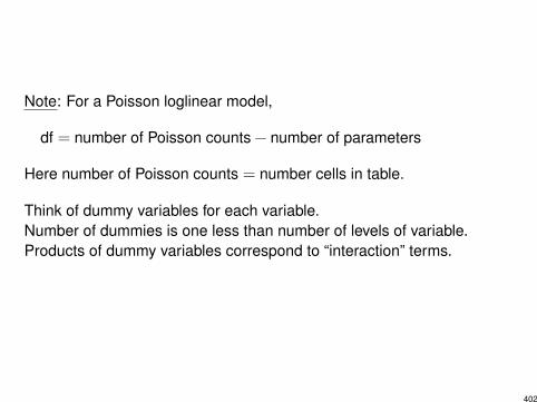
(Dispersion parameter for poisson family taken to be 1)

Null deviance: 90.242 on 15 degrees of freedom

Residual deviance: 13.467 on 9 degrees of freedom

AIC: 77.07

Number of Fisher Scoring iterations: 5

NA

> chisqstat(jobsat.indep)

[1] 11.524

411

> jobsat.saturated <- update(jobsat.indep, . ~ Income*Satis)

> anova(jobsat.indep, jobsat.saturated, test="Chisq")

Analysis of Deviance Table

Model 1: Freq ~ Income + Satis

Model 2: Freq ~ Income + Satis + Income:Satis

Resid. Df Resid. Dev Df Deviance Pr(>Chi)

1 9 13.5

2 0 0.0 9 13.5 0.14

> ## Set contrasts back to R defaults

> options(contrasts=c("contr.treatment","contr.poly"))

412

Loglinear Models for Three-Way TablesHere two-factor terms represent conditional log odds ratios at a fixedlevel of the third variable.

Ex. 2 ⇥ 2 ⇥ 2 table. Consider the model

log(µijk

) = �+ �

X

i

+ �

Y

j

+ �

Z

k

+ �

XZ

ik

+ �

YZ

jk

.

Called the model of X-Y conditional independence; denoted (XZ, YZ).

IX and Y are conditionally independent, given Z:

log(✓XY(k)) = 0 =) ✓

XY(k) = 1

I the X-Z odds ratio is the same at all levels of Y:

log(✓X(j)Z) = �

XZ

11 + �

XZ

22 - �

XZ

12 - �

XZ

21| {z }does not depend on j

Similarly, Y-Z odds ratio same at all levels of X. Model has nothree-factor interaction.

413

Ex. Consider the loglinear model

log(µijk

) = �+ �

X

i

+ �

Y

j

+ �

Z

k

+ �

XY

ij

+ �

XZ

ik

+ �

YZ

jk

.

Each pair of variables is conditionally dependent, but association (asmeasured by odds ratios) is the same at all levels of third variable.

Called the model of homogeneous association (or model of nothree-factor interaction; denoted (XY,XZ, YZ).

414

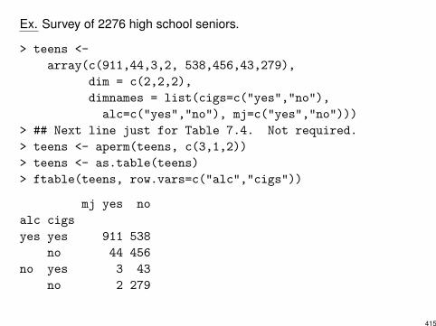
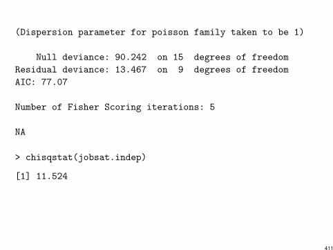
Ex. Survey of 2276 high school seniors.

> teens <-

array(c(911,44,3,2, 538,456,43,279),

dim = c(2,2,2),

dimnames = list(cigs=c("yes","no"),

alc=c("yes","no"), mj=c("yes","no")))

> ## Next line just for Table 7.4. Not required.

> teens <- aperm(teens, c(3,1,2))

> teens <- as.table(teens)

> ftable(teens, row.vars=c("alc","cigs"))

mj yes no

alc cigs

yes yes 911 538

no 44 456

no yes 3 43

no 2 279

415

> teens.df <- as.data.frame(teens)

> teens.df

mj cigs alc Freq

1 yes yes yes 911

2 no yes yes 538

3 yes no yes 44

4 no no yes 456

5 yes yes no 3

6 no yes no 43

7 yes no no 2

8 no no no 279

> teens.df <-

transform(teens.df,

cigs = relevel(cigs, "no"),

alc = relevel(alc, "no"),

mj = relevel(mj, "no"))

416

> teens.AC.AM.CM <-

glm(Freq ~ alc*cigs + alc*mj + cigs*mj,

family=poisson, data=teens.df)

> ### Another way:

> ## teens.AC.AM.CM <-

> ## glm(Freq ~ alc*cigs*mj - alc:cigs:mj,

> ## family=poisson, data=teens.df)

> summary(teens.AC.AM.CM)

417

Call:

glm(formula = Freq ~ alc * cigs + alc * mj + cigs * mj, family = poisson,

data = teens.df)

Coefficients:

Estimate Std. Error z value Pr(>|z|)

(Intercept) 5.6334 0.0597 94.36 < 2e-16

alcyes 0.4877 0.0758 6.44 1.2e-10

cigsyes -1.8867 0.1627 -11.60 < 2e-16

mjyes -5.3090 0.4752 -11.17 < 2e-16

alcyes:cigsyes 2.0545 0.1741 11.80 < 2e-16

alcyes:mjyes 2.9860 0.4647 6.43 1.3e-10

cigsyes:mjyes 2.8479 0.1638 17.38 < 2e-16

(Dispersion parameter for poisson family taken to be 1)

Null deviance: 2851.46098 on 7 degrees of freedom

Residual deviance: 0.37399 on 1 degrees of freedom

AIC: 63.42

418

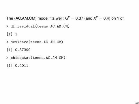
The (AC,AM,CM) model fits well: G2 = 0.37 (and X

2 = 0.4) on 1 df.

> df.residual(teens.AC.AM.CM)

[1] 1

> deviance(teens.AC.AM.CM)

[1] 0.37399

> chisqstat(teens.AC.AM.CM)

[1] 0.4011

419

Note: As a LRT, goodness-of-fit on previous slide is comparing tosaturated model.

> teens.ACM <- update(teens.AC.AM.CM, . ~ alc*cigs*mj)

> anova(teens.AC.AM.CM, teens.ACM, test="Chisq")

Analysis of Deviance Table

Model 1: Freq ~ alc * cigs + alc * mj + cigs * mj

Model 2: Freq ~ alc + cigs + mj + alc:cigs + alc:mj + cigs:mj + alc:cigs:mj

Resid. Df Resid. Dev Df Deviance Pr(>Chi)

1 1 0.374

2 0 0.000 1 0.374 0.54

420

And none of the interaction terms can be dropped:

> drop1(teens.AC.AM.CM, test="Chisq")

Single term deletions

Model:

Freq ~ alc * cigs + alc * mj + cigs * mj

Df Deviance AIC LRT Pr(>Chi)

<none> 0 63

alc:cigs 1 188 249 187 <2e-16

alc:mj 1 92 153 92 <2e-16

cigs:mj 1 497 558 497 <2e-16

421

Note: drop1() does LRTs comparing to simpler models. Test statistic isthe usual

-2(L0 - L1) = deviance0 - deviance1

and df is difference in number of nonredundant parameters.

E.g., to test for conditional independence of A and C given M:

> teens.AM.CM <- update(teens.AC.AM.CM, . ~ alc*mj + cigs*mj)

> anova(teens.AM.CM, teens.AC.AM.CM, test="Chisq")

Analysis of Deviance Table

Model 1: Freq ~ alc + mj + cigs + alc:mj + mj:cigs

Model 2: Freq ~ alc * cigs + alc * mj + cigs * mj

Resid. Df Resid. Dev Df Deviance Pr(>Chi)

1 2 187.8

2 1 0.4 1 187 <2e-16

422

Table 7.4 gives fitted values for several different models fit to these data.

> teens.AM.CM <-update(teens.AC.AM.CM, . ~ alc*mj + cigs*mj)

> teens.AC.M <-update(teens.AC.AM.CM, . ~ alc*cigs + mj)

> teens.A.C.M <-update(teens.AC.AM.CM, . ~ alc + cigs + mj)

> teens.ACM <-update(teens.AC.AM.CM, . ~ alc*cigs* mj)

> table.7.4 <-data.frame(predict(teens.A.C.M, type="response"))

> table.7.4 <-cbind(table.7.4, predict(teens.AC.M, type="response"))

> table.7.4 <-cbind(table.7.4, predict(teens.AM.CM, type="response"))

> table.7.4 <-cbind(table.7.4, predict(teens.AC.AM.CM, type="response"))

> table.7.4 <-cbind(table.7.4, predict(teens.ACM, type="response"))

423

> table.7.4 <- signif(table.7.4, 3)

> table.7.4 <-

cbind(teens.df[,c("alc","cigs","mj")],

table.7.4)

> names(table.7.4) <-

c("alc","cigs","mj",

"(A,C,M)","(AC,M)","(AM,CM)","(AC,AM,CM)","(ACM)")

424

> table.7.4

alc cigs mj (A,C,M) (AC,M) (AM,CM) (AC,AM,CM) (ACM)

1 yes yes yes 540.0 611.0 909.00 910.00 911

2 yes yes no 740.0 838.0 439.00 539.00 538

3 yes no yes 282.0 211.0 45.80 44.60 44

4 yes no no 387.0 289.0 555.00 455.00 456

5 no yes yes 90.6 19.4 4.76 3.62 3

6 no yes no 124.0 26.6 142.00 42.40 43

7 no no yes 47.3 119.0 0.24 1.38 2

8 no no no 64.9 162.0 180.00 280.00 279

425

In (AC,AM,CM) model, AC odds-ratio is the same at each level of M.With 1 = yes and 2 = no for each variable, the estimated conditional ACodds ratio is

µ̂11kµ̂22k

µ̂12kµ̂21k= exp

⇣�̂

AC11 + �̂

AC22 - �̂

AC12 - �̂

AC21

⌘= e

2.0545 = 7.8

A 95% CI is

e

2.05±(1.96)(0.174) =�e

1.71, e2.40� = (5.5, 11.0)

The commons odds-ratio is reflected in the fitted values for the model:

(910)(1.38)(44.6)(3.62)

= 7.8(539)(280)(455)(42.4)

= 7.8

Similar results hold for AM and CM conditional odds-ratios in this model.

426

In (AM,CM) model, �ACij

= 0, and conditional AC odds-ratio (given M) ise

0 = 1 at each level of M, i.e., A and C are conditionally indep. given M.Again, this is reflected in the fitted values for this model.

(909)(0.24)(45.8)(4.76)

= 1(439)(180)(555)(142)

= 1

The AM odds-ratio is not 1, but it is the same at each level of C:

(909)(142)(439)(4.76)

= 61.87(45.8)(180)(555)(0.24)

= 61.87

Similarly, the CM odds-ratio is the same at each level of A:

(909)(555)(439)(45.8)

= 25.14(4.76)(180)(142)(0.24)

= 25.14

427

Standardized residuals may help understand lack of fit.Text uses standardized Pearson residuals.rstandard() computes standardized deviance resids. by defaultbut has type = "pearson" option.

See Section 7.2.2 for example and discussion.

428

Note:

I Loglinear models extend to any number of dimensions.

I Loglinear models treat all variables symmetrically.

Logistic regression models treat Y as response and other variablesas explanatory. More natural approach when there is a singleresponse.

429

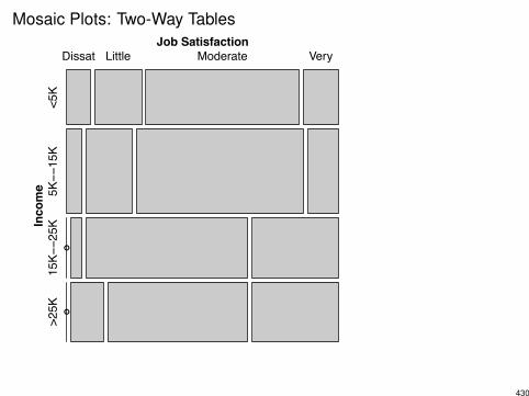
Mosaic Plots: Two-Way Tables

●

●

Job SatisfactionIn

com

e>25K

15K−−25K

5K−−15K

<5K

Dissat Little Moderate Very

430

The previous plot was produced by the commands

> library(vcd)

> mosaic(sattab)

The same plot could have been produced with

> mosaic(~ Income + Satis, data = jobsat)

You might prefer to view the plot with a different orientation:

> mosaic(sattab, split_vertical = TRUE)

431

● ●

IncomeJo

b Sa

tisfa

ctio

n<5KVery

Moderate

Little

Dissat

5K−−15K 15K−−25K >25K

432

Recall:

> (sat.chisq <- chisq.test(sattab))

Pearson's Chi-squared test

data: sattab

X-squared = 11.524, df = 9, p-value = 0.2415

> round(sat.chisq$expected, 1)

Job Satisfaction

Income Dissat Little Moderate Very

<5K 0.8 3.0 13.3 4.9

5K--15K 1.3 4.6 20.6 7.5

15K--25K 0.9 3.2 14.5 5.3

>25K 0.9 3.2 14.5 5.3

> mosaic(sattab, split_vertical = TRUE, main = "Observed")

> mosaic(sattab, split_vertical = TRUE, type = "expected",

main = "Expected")433

Observed

● ●

Income

Job

Satis

fact

ion

<5K

Very

Moderate

LittleDissat 5K−−15K 15K−−25K >25K

ExpectedIncome

Job

Satis

fact

ion

<5K

Very

Moderate

LittleDissat 5K−−15K 15K−−25K >25K

434

> round(sat.chisq$stdres, 1)

Job Satisfaction

Income Dissat Little Moderate Very

<5K 1.4 0.7 -0.2 -1.1

5K--15K 0.8 0.9 0.6 -1.8

15K--25K -1.1 -1.5 0.2 1.5

>25K -1.1 -0.2 -0.7 1.5

Same as the standardized (i.e., ”adjusted”) Pearson residuals fromfitting loglinear model of independence:

> round(rstandard(jobsat.indep, type = "pearson"), 1)

1 2 3 4 5 6 7 8 9 10 11

1.4 0.8 -1.1 -1.1 0.7 0.9 -1.5 -0.2 -0.2 0.6 0.2

12 13 14 15 16

-0.7 -1.1 -1.8 1.5 1.5

435

This example isn’t the best here because Pearson’s chi-square testdoes not provide any evidence against independence.

> mosaic(sattab, gp = shading_Friendly)

> mosaic(sattab, residuals = sat.chisq$stdres,

gp = shading_hcl,

gp_args = list(p.value = sat.chisq$p.value,

interpolate = c(2,4)))

436

−1.28

0.00

1.25

Pearsonresiduals:

●●

●●

Job SatisfactionIn

com

e>2

5K15

K−−2

5K5K−−

15K

<5K

DissatLittle Moderate Very

437

−1.77

0.00

1.51

p−value =0.241

●●

●●

Job SatisfactionIn

com

e>2

5K15

K−−2

5K5K−−

15K

<5K

DissatLittle Moderate Very

438

Hair and Eye Color

Data from vcd package.

> ftable(Eye ~ Sex + Hair, data = HairEyeColor)

Eye Brown Blue Hazel Green

Sex Hair

Male Black 32 11 10 3

Brown 53 50 25 15

Red 10 10 7 7

Blond 3 30 5 8

Female Black 36 9 5 2

Brown 66 34 29 14

Red 16 7 7 7

Blond 4 64 5 8

439

Hair and Eye Color (ctd)

Collapsing across Sex.

> haireye <- margin.table(HairEyeColor, 1:2)

> haireye

Eye

Hair Brown Blue Hazel Green

Black 68 20 15 5

Brown 119 84 54 29

Red 26 17 14 14

Blond 7 94 10 16

> (he.chisq <- chisq.test(haireye))

Pearson's Chi-squared test

data: haireye

X-squared = 138.29, df = 9, p-value < 2.2e-16

440

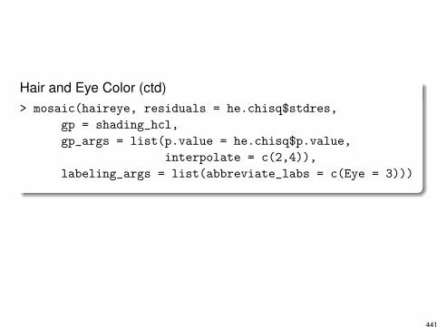
Hair and Eye Color (ctd)> mosaic(haireye, residuals = he.chisq$stdres,

gp = shading_hcl,

gp_args = list(p.value = he.chisq$p.value,

interpolate = c(2,4)),

labeling_args = list(abbreviate_labs = c(Eye = 3)))

441

−8.33

−4.00−2.00 0.00 2.00 4.00

9.97

p−value =<2e−16

EyeHair

Blon

dR

edBr

own

Blac

kBrw Blu Hzl Grn

442

Teen Survey Datacigsmj

alc

no

noyes

yes

yes no

noyes

443

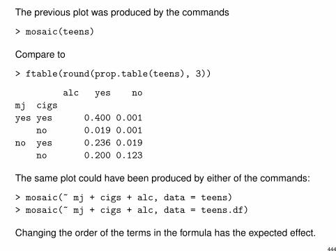
The previous plot was produced by the commands

> mosaic(teens)

Compare to

> ftable(round(prop.table(teens), 3))

alc yes no

mj cigs

yes yes 0.400 0.001

no 0.019 0.001

no yes 0.236 0.019

no 0.200 0.123

The same plot could have been produced by either of the commands:

> mosaic(~ mj + cigs + alc, data = teens)

> mosaic(~ mj + cigs + alc, data = teens.df)

Changing the order of the terms in the formula has the expected effect.444

Standardized residuals from two loglinear models.

> table.7.8 <- teens.df[,c("alc","cigs","mj","Freq")]> table.7.8 <- cbind(table.7.8,

round(predict(teens.AM.CM, type = "response"),1))> table.7.8 <- cbind(table.7.8,

round(rstandard(teens.AM.CM, type = "pearson"),2))> table.7.8 <- cbind(table.7.8,

round(predict(teens.AC.AM.CM, type = "response"),1))> table.7.8 <- cbind(table.7.8,

round(rstandard(teens.AC.AM.CM, type = "pearson"),2))> names(table.7.8) <-

c("A","C","M","Obs","(AM,CM)","StdRes","(AC,AM,CM)","StdRes")

445

> table.7.8

A C M Obs (AM,CM) StdRes (AC,AM,CM) StdRes

1 yes yes yes 911 909.2 3.7 910.4 0.63

2 yes yes no 538 438.8 12.8 538.6 -0.63

3 yes no yes 44 45.8 -3.7 44.6 -0.63

4 yes no no 456 555.2 -12.8 455.4 0.63

5 no yes yes 3 4.8 -3.7 3.6 -0.63

6 no yes no 43 142.2 -12.8 42.4 0.63

7 no no yes 2 0.2 3.7 1.4 0.63

8 no no no 279 179.8 12.8 279.6 -0.63

I Number nonredundant standardized residuals = residual df.

I Model (AM,CM): Residual df = 2

I Model (AC,AM,CM): Residual df = 1

446

vcdExtra package works from fitted loglinear model.Uses unadjusted Pearson residuals, or optionally, standardizeddeviance residuals.

Here is the default, using unadjusted Pearson residuals:

> library(vcdExtra)

> mosaic(teens.AM.CM, ~ mj + cigs + alc)

> mosaic(teens.AC.AM.CM, ~ mj + cigs + alc)

447

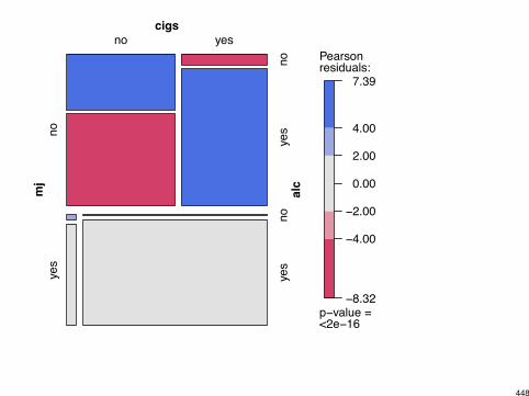
−8.32

−4.00

−2.00

0.00

2.00

4.00

7.39

Pearsonresiduals:

p−value =<2e−16

cigsmj

alc

yes

yes

no

nono yes

yes

no

448

−0.324

0.000

0.524

Pearsonresiduals:

p−value =0.527

cigsmj

alc

yes

yes

no

nono yes

yes

no

449

With the standardized deviance residuals:

> mosaic(teens.AM.CM, ~ mj + cigs + alc,

residuals_type = "rstandard")

> mosaic(teens.AC.AM.CM, ~ mj + cigs + alc,

residuals_type = "rstandard")

450

−15.0

−4.0 −2.0 0.0 2.0 4.0

12.4rstandard

p−value =<2e−16

cigsmj

alc

yes

yes

no

nono yes

yes

no

451

−0.653

0.000

0.633rstandard

p−value =0.0743

cigsmj

alc

yes

yes

no

nono yes

yes

no

452

And finally, with the standardized Pearson residuals (note that the titleon the legend is not correct):

> mosaic(teens.AM.CM, ~ mj + cigs + alc,

residuals = rstandard(teens.AM.CM, type = "pearson"))

> mosaic(teens.AC.AM.CM, ~ mj + cigs + alc,

residuals = rstandard(teens.AC.AM.CM, type = "pearson"))

I have suggested a patch to make the selection of Pearson vs devianceand non-standardized vs standardized residuals more straightforward.

453

−12.8

−4.0 −2.0 0.0 2.0 4.0

12.8

Pearsonresiduals:

p−value =<2e−16

cigsmj

alc

yes

yes

no

nono yes

yes

no

454

−0.633

0.000

0.633

Pearsonresiduals:

p−value =0.0732

cigsmj

alc

yes

yes

no

nono yes

yes

no

455

7.3 The Loglinear-Logit Connection

The loglinear model (XY,XZ, YZ), i.e.,

log(µijk

) = �+ �

X

i

+ �

Y

j

+ �

Z

k

+ �

XY

ij

+ �

XZ

ik

+ �

YZ

jk

,

I treats variables symmetrically

I permits association for each pair of vars.

I allows no three-factor association (i.e., implies homogeneousassociation)

456

Suppose Y is binary and let

⇡

ik

= P(Y = 1|X = i,Z = k).

Treat Y as response. If model (XY,XZ, YZ) holds, then

logit(⇡ik

) = log⇣

⇡

ik

1 - ⇡

ik

⌘= log

⇣P(Y = 1|X = i,Z = k)

P(Y = 2|X = i,Z = k)

⌘

= log(µi1k)- log(µ

i2k)

= (�+ �

X

i

+ �

Y

1 + �

Z

k

+ �

XY

i1 + �

XZ

ik

+ �

YZ

1k )

- (�+ �

X

i

+ �

Y

2 + �

Z

k

+ �

XY

i2 + �

XZ

ik

+ �

YZ

2k )

= (�Y1 - �

Y

2 )| {z }↵

+(�XY

i1 - �

XY

i2 )| {z }�

X

i

+(�YZ

1k - �

YZ

2k )| {z }�

Z

k

= ↵+ �

X

i

+ �

Z

k

i.e., logit model for Y has additive main effects and no interaction.

457

UCB Admissions

Recall the UCB admissions data.

Gender Male Female

Admit Admitted Rejected Admitted Rejected

Dept

A 512 313 89 19

B 353 207 17 8

C 120 205 202 391

D 138 279 131 244

E 53 138 94 299

F 22 351 24 317

Let A = admission (yes/no) be response var. Logit model:

logit(⇡ik

) = ↵+ �

G

i

+ �

D

k

The corresponding loglinear model is (AG,AD,DG):

log(µijk

) = �+ �

A

i

+ �

G

j

+ �

D

k

+ �

AG

ij

+ �

AD

ik

+ �

DG

jk

458

UCB Admissions (ctd)

Both models have deviance G

2 = 20.20 (df = 5):

> UCB.logit <-

glm(cbind(Admitted, Rejected) ~ Gender + Dept,

family = binomial, data = UCBw)

> c(deviance(UCB.logit), df.residual(UCB.logit))

[1] 20.204 5.000

> UCB.loglin <-

glm(Freq ~ Admit*Gender + Admit*Dept + Gender*Dept,

family = poisson, data = UCBdf)

> c(deviance(UCB.loglin), df.residual(UCB.loglin))

[1] 20.204 5.000

459

UCB Admissions (ctd)

The df for testing fit are the same for each model:

Logit model Treats table as indep. binomial variates on responseA at 12 combinations of levels of D and G:

no. obs. =

no. param. =

(residual) df =

Loglinear model Treats table as 24 indep. Poisson variates:

no. obs. =

no. param. =

(residual) df =

460

UCB Admissions (ctd)

Controlling for D (department), estimated odds ratio for effected of G onA (odds of admission for males divided by odds for females), is

exp(�̂G

1 - �̂

G

2 ) = = .905

Identical to

exp��̂

AG

11 + �̂

AG

22 - �̂

AG

12 - �̂

AG

21�=

> coef(UCB.logit)

(Intercept) GenderFemale DeptB DeptC

0.582051 0.099870 -0.043398 -1.262598

DeptD DeptE DeptF

-1.294606 -1.739306 -3.306480

461

> coef(UCB.loglin)

(Intercept) AdmitRejected

6.271499 -0.582051

GenderFemale DeptB

-1.998588 -0.403220

DeptC DeptD

-1.577903 -1.350005

DeptE DeptF

-2.449820 -3.137871

AdmitRejected:GenderFemale AdmitRejected:DeptB

-0.099870 0.043398

AdmitRejected:DeptC AdmitRejected:DeptD

1.262598 1.294606

AdmitRejected:DeptE AdmitRejected:DeptF

1.739306 3.306480

GenderFemale:DeptB GenderFemale:DeptC

-1.074820 2.665133

GenderFemale:DeptD GenderFemale:DeptE

1.958324 2.795186

GenderFemale:DeptF

2.002319

462

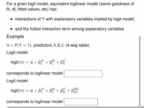
For a given logit model, equivalent loglinear model (same goodness offit, df, fitted values, etc) has:

I interactions of Y with explanatory variables implied by logit model;

I and the fullest interaction term among explanatory variables

Example

⇡ = P(Y = 1), predictors A,B,C (4-way table).

Logit model

logit(⇡) = ↵+ �

A

i

+ �

B

j

+ �

C

k

corresponds to loglinear model .

Logit model

logit(⇡) = ↵+ �

A

i

+ �

B

j

+ �

C

k

+ �

BC

jk

corresponds to loglinear model .463

Remarks

I When there is a single binary response, it is simpler to approachdata directly using logit models.

I Similar remarks hold for a multi-category response Y:I Baseline-category logit model has a matching loglinear model.I With a single response, it is simpler to use the baseline-category

logit model.

I Loglinear models have advantage of generality — can handlemultiple responses, some of which may have more than twooutcome categories.

464

7.4 Independence Graphs and Collapsibility

Independence graph: a graphical representation for conditionalindependence.

I Vertices (or nodes) represent variables.

I Connected by edges: a missing edge between two variablesrepresents a conditional independence between the variables.

I Different models may produce the same graph.

I Graphical models: subclass of loglinear models

I Within this class there is a unique model for each independencegraph.

I For any group of variables having no missing edges, graphical modelcontains the highest order interaction term for those variables.

465

Independence Graphs for a 4-Way Table (Variables W, X, Y, Z)

Model(s) Graph

(WX,WY,WZ, YZ)(WX,WYZ)⇤ X W

Y

Z(WX,WY,WZ,XZ, YZ)

(WX,XZ,WYZ)(WXZ,WY, YZ)(WXZ,WYZ)⇤

X

W

Z

Y

(WX,WY,WZ)⇤ X W

Y

Z(WX,XY, YZ)⇤ W X Y Z

⇤ Graphical models.

466

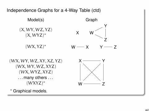
Independence Graphs for a 4-Way Table (ctd)

Model(s) Graph

(X,WY,WZ, YZ)(X,WYZ)⇤ X W

Y

Z(WX, YZ)⇤ W X Y Z

(WX,WY,WZ,XY,XZ, YZ)(WX,WY,WZ,XYZ)(WX,WYZ,XYZ). . . many others . . .

(WXYZ)⇤ W

X Y

Z⇤ Graphical models.

467

Collapsibility Conditions for Three-Way Tables

For a three-way table, the XY marginal and conditional oddsratios are identical if either Z and X are conditonallyindependent or if Z and Y are conditionally independent.

I Conditions say control variable Z is either:

I conditionally independent of X given Y, as in model (XY, YZ);

I or conditionally independent of Y given X, as in (XY,XZ).

I I.e., XY association is identical in the partial tables and themarginal table for models with independence graphs

X Y Z Y X Z

or even simpler models.

468

Teen Survey

A = alcohol use, C = cigarette use, M = marijuana use.

The model of AC conditional independence, (AM,CM), hasindependence graph

A M C

Consider AM association, treating C as control variable.Since C is conditionally independent of A, the AM conditional oddsratios are the same as the AM marginal odds ratio collapsed over C.

(909.24)(142.16)(438.84)(4.76)

=(45.76)(179.84)(555.16)(0.24)

=(955)(322)(994)(5)

= 61.9

See Tables 7.4 and 7.5, or next slide.

> exp(coef(teens.AM.CM)[5])

alcyes:mjyes

61.873

469

> AM.CM.fitted <- teens

> AM.CM.fitted[,,] <- predict(teens.AM.CM, type="response")

> AM.CM.fitted[,"yes",]

alc

mj yes no

yes 909.24 4.7604

no 438.84 142.1596

> AM.CM.fitted[,"no",]

alc

mj yes no

yes 45.76 0.23958

no 555.16 179.84043

> AM.CM.fitted[,"yes",] + AM.CM.fitted[,"no",]

alc

mj yes no

yes 955 5

no 994 322470

Teen Survey

I Similarly, CM association is collapsible over A.I The AC association is not collapsible, because M is conditionally

dependent with both A and C in model (AM,CM).

Thus, A and C may be marginally dependent, even thoughconditionally independent.

(909.24)(0.24)(45.76)(4.76)

=(438.84)(179.84)(555.16)(142.16)

=

(1348.08)(180.08)(600.92)(146.92)

= 2.75 6= 1

471

> AM.CM.fitted["yes",,]

alc

cigs yes no

yes 909.24 4.76042

no 45.76 0.23958

> AM.CM.fitted["no",,]

alc

cigs yes no

yes 438.84 142.16

no 555.16 179.84

> AM.CM.fitted["yes",,] + AM.CM.fitted["no",,]

alc

cigs yes no

yes 1348.08 146.92

no 600.92 180.08

472

Collapsibility Conditions for Multiway Tables

If the variables in a model for a multiway table partition intothree mutually exclusive subsets, A, B, C, such that Bseparates A and C (that is, if the model does not containparameters linking variables from A directly to variables fromC), then when the table is collapsed over the variables in C,model parameters relating variables in A and modelparameters relating variables in A with variables in B areunchanged.

A B C

473

Teen Survey Data> data(teens)

> ftable(R + G + M ~ A + C, data = teens)

R White Other

G Female Male Female Male

M Yes No Yes No Yes No Yes No

A C

Yes Yes 405 268 453 228 23 23 30 19

No 13 218 28 201 2 19 1 18

No Yes 1 17 1 17 0 1 1 8

No 1 117 1 133 0 12 0 17

474

Teen Survey Data (ctd)

Text suggests loglinear model (AC, AM, CM, AG, AR, GM, GR).

C

M

A

G

R

The set {A, M} separates sets {C} and {G, R}.I.e., C is conditionally independent of G and R given M and A.Thus (as verified on the next slide):

Collapsing over G and R, the conditional associations betweenC and M and between C and A are the same as with themodel (AC, AM, CM) fitted earlier.

> teens.df <- as.data.frame(teens)

> ACM <- margin.table(teens, 1:3)

> ACM.df <- as.data.frame(ACM)

475

> teens.m6 <-

glm(Freq ~ A*C + A*M + C*M + A*G + A*R + G*M + G*R,

family = poisson, data = teens.df)

> AC.AM.CM <- glm(Freq ~ A*C + A*M + C*M,

family = poisson, data = ACM.df)

> coef(teens.m6)

(Intercept) ANo CNo MNo

5.97841 -5.75073 -3.01575 -0.38955

GMale ROther ANo:CNo ANo:MNo

0.13584 -2.66305 2.05453 3.00592

CNo:MNo ANo:GMale ANo:ROther MNo:GMale

2.84789 0.29229 0.59346 -0.26929

GMale:ROther

0.12619

> coef(AC.AM.CM)

(Intercept) ANo CNo MNo

6.81387 -5.52827 -3.01575 -0.52486

ANo:CNo ANo:MNo CNo:MNo

2.05453 2.98601 2.84789

476