Ch-4 Production Theory
45
Ch 4 THE THEORY OF PRODUCTION Production theory forms the foundation for the theory of supply Managerial decision making involves four types of production decisions: 1. Whether to pro duce or to shut down 2. How much ou tput t o pr oduce 3. What i nput combi nati on to use 4. What type of technology to use Ch 5 Ch 4
-
Upload
jituhirapara1990 -
Category
Documents
-
view
221 -
download
0
Transcript of Ch-4 Production Theory

8/6/2019 Ch-4 Production Theory
http://slidepdf.com/reader/full/ch-4-production-theory 1/45
Ch 4 THE THEORY OFPRODUCTION
Production theory forms thefoundation for the theory of supply
Managerial decision making involvesfour types of production decisions:
1. Whether to produce or to shut
down
2. How much output to produce
3. What input combination to use
4. What type of technology to use
Ch 5
Ch 4

8/6/2019 Ch-4 Production Theory
http://slidepdf.com/reader/full/ch-4-production-theory 2/45
Production involves transformation
of inputs such as capital,
equipment, labor, and land into
output - goods and services
In this production process, the
manager is concerned with
efficiency in the use of the inputs
- technical vs. economical
efficiency

8/6/2019 Ch-4 Production Theory
http://slidepdf.com/reader/full/ch-4-production-theory 3/45
Two Concepts of Efficiency
Economic efficiency:
occurs when the cost of producing
a given output is as low as possible
Technological efficiency:
occurs when it is not possible to
increase output without increasing
inputs
8/6/2019 Ch-4 Production Theory
http://slidepdf.com/reader/full/ch-4-production-theory 4/45
The objective of efficiency willprovide us with some basic rules
about the manner in which firms
should utilize inputs to produce
goods and services

8/6/2019 Ch-4 Production Theory
http://slidepdf.com/reader/full/ch-4-production-theory 5/45
You will see that basic productiontheory is simply an application of
constrained optimization:the firm attempts either to minimizethe cost of producing a given levelof output
or
to maximize the output attainablewith a given level of cost.
Both optimization problems lead tosame rule for the allocation of inputs and choice of technology

8/6/2019 Ch-4 Production Theory
http://slidepdf.com/reader/full/ch-4-production-theory 6/45
Production Function
A production function is a table or amathematical equation showing themaximum amount of output that can beproduced from any specified set of inputs,
given the existing technology
f 2(x)f
1(x)
f 0(x)
x
Q Improvement of technology
f 0
(x) - f 2
(x)
Q = output
x = inputs

8/6/2019 Ch-4 Production Theory
http://slidepdf.com/reader/full/ch-4-production-theory 7/45
Production Function continued
Q = f(X1, X
2, …, X
k)
where
Q = output
X1, …, X
k= inputs
For our current analysis, let’s reduce theinputs to two, capital (K) and labor (L):
Q = f(L, K)

8/6/2019 Ch-4 Production Theory
http://slidepdf.com/reader/full/ch-4-production-theory 8/45
Production Table
Units of K Employed Output Quantity (Q)
8 37 60 83 96 107 117 127 128
7 42 64 78 90 101 110 119 120
6 37 52 64 73 82 90 97 104
5 31 47 58 67 75 82 89 954 24 39 52 60 67 73 79 85
3 17 29 41 52 58 64 69 73
2 8 18 29 39 47 52 56 52
1 4 8 14 20 27 24 21 17
1 2 3 4 5 6 7 8
Units of L Employed
Same Q can be produced with differentcombinations of inputs, e.g. inputs are substitutable
in some degree
8/6/2019 Ch-4 Production Theory
http://slidepdf.com/reader/full/ch-4-production-theory 9/45
All of these outputs are assumed to
be technically efficient
But which one is economically efficient?
That is the question facing the DM

8/6/2019 Ch-4 Production Theory
http://slidepdf.com/reader/full/ch-4-production-theory 10/45
Types of Production Functions
Production function with one variable
input
Production function with two variable
inputs Production function with all variable
inputs
8/6/2019 Ch-4 Production Theory
http://slidepdf.com/reader/full/ch-4-production-theory 11/45
Short-Run and Long-Run Production
In the short run some inputs are
fixed and some variable
e.g. the firm may be able to vary
the amount of labor, but cannotchange the amount of capital
in the short run we can talk about
factor productivity

8/6/2019 Ch-4 Production Theory
http://slidepdf.com/reader/full/ch-4-production-theory 12/45
In the long run all inputs become
variable e.g. the long run is the period in
which a firm can adjust all inputsto changed conditions
in the long run we can talk aboutreturns to scale (compare latter
with economies of scale, which
is a cost related concept)
8/6/2019 Ch-4 Production Theory
http://slidepdf.com/reader/full/ch-4-production-theory 13/45
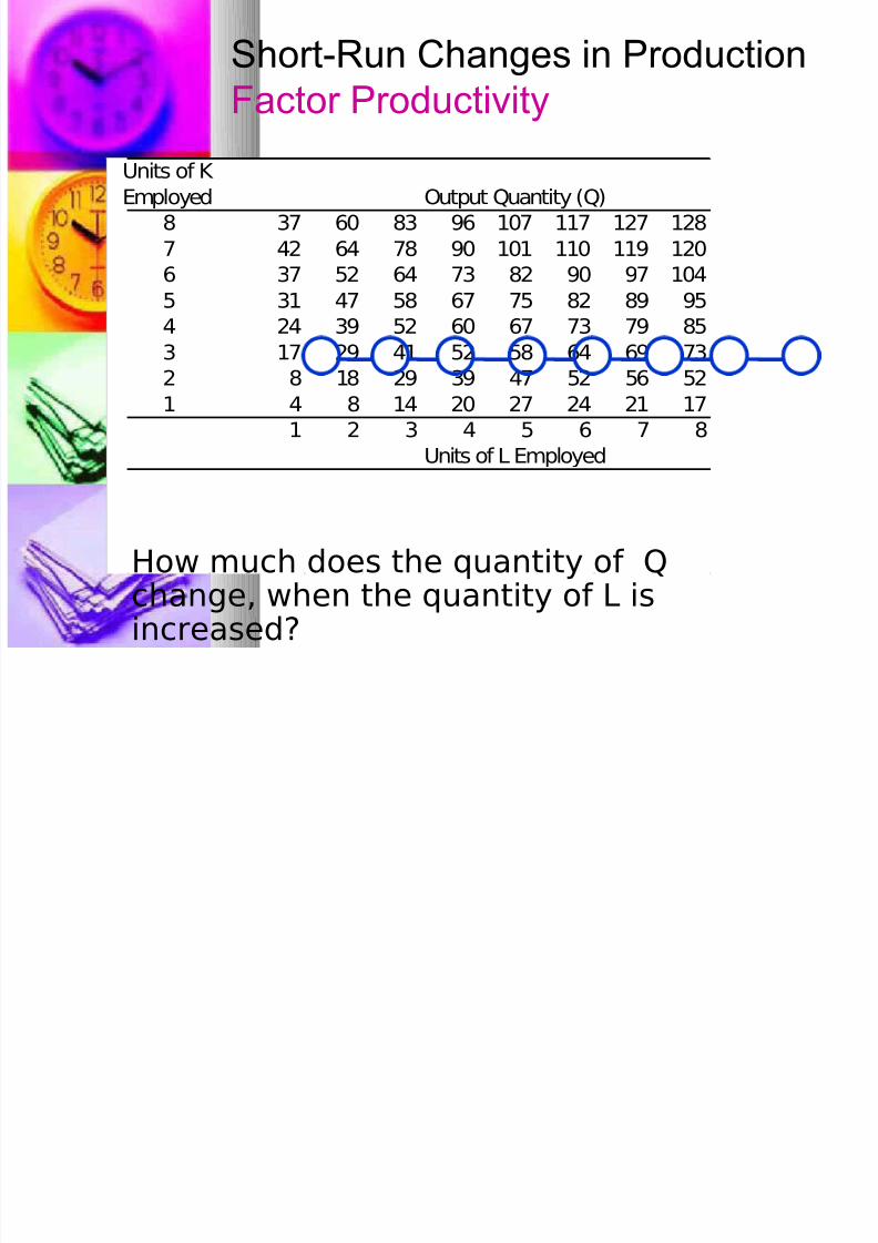
Short-Run Changes in Production
Factor Productivity
Units of K
Employed Output Quantity (Q)
8 37 60 83 96 107 117 127 128
7 42 64 78 90 101 110 119 120
6 37 52 64 73 82 90 97 104
5 31 47 58 67 75 82 89 954 24 39 52 60 67 73 79 85
3 17 29 41 52 58 64 69 73
2 8 18 29 39 47 52 56 52
1 4 8 14 20 27 24 21 17
1 2 3 4 5 6 7 8
Units of L Employed
How much does the quantity of Q
change, when the quantity of L isincreased?

8/6/2019 Ch-4 Production Theory
http://slidepdf.com/reader/full/ch-4-production-theory 14/45
Long-Run Changes in Production
Returns to Scale
Units of K
Employed Output Quantity (Q)
8 37 60 83 96 107 117 127 128
7 42 64 78 90 101 110 119 120
6 37 52 64 73 82 90 97 104
5 31 47 58 67 75 82 89 954 24 39 52 60 67 73 79 85
3 17 29 41 52 58 64 69 73
2 8 18 29 39 47 52 56 52
1 4 8 14 20 27 24 21 17
1 2 3 4 5 6 7 8
Units of L Employed
How much does the quantity of Q change,when the quantity of both L and K is
increased?

8/6/2019 Ch-4 Production Theory
http://slidepdf.com/reader/full/ch-4-production-theory 15/45
Relationship Between Total, Average,and Marginal Product: Short-Run
Analysis
Total Product (TP) = total quantity of
output
Average Product (AP) = total product
per total input
Marginal Product (MP) = change in
quantity when one additional unit of
input used
8/6/2019 Ch-4 Production Theory
http://slidepdf.com/reader/full/ch-4-production-theory 16/45
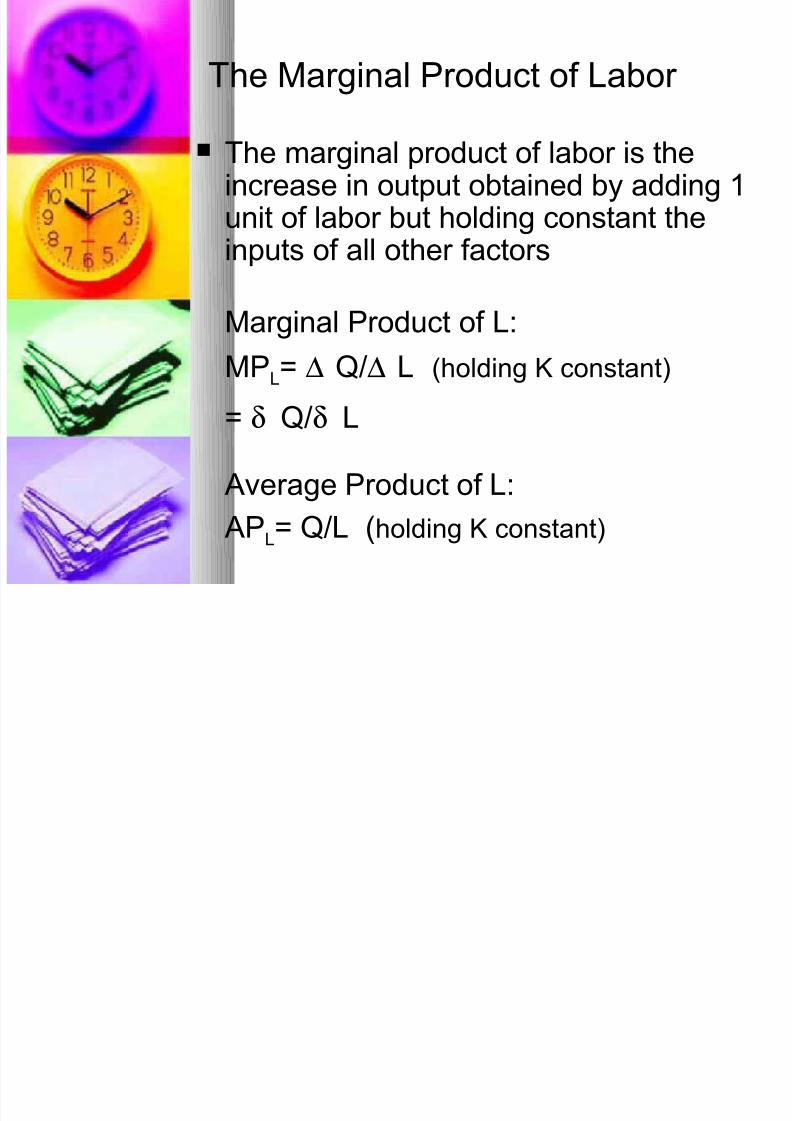
The Marginal Product of Labor
The marginal product of labor is theincrease in output obtained by adding 1unit of labor but holding constant theinputs of all other factors
Marginal Product of L:
MPL= ∆ Q/∆ L (holding K constant)
= δ Q/δ L
Average Product of L:
APL= Q/L (holding K constant)

8/6/2019 Ch-4 Production Theory
http://slidepdf.com/reader/full/ch-4-production-theory 17/45
Short-Run Analysis of Total,Average, and Marginal Product
If MP > AP thenAP is rising
If MP < AP thenAP is falling
MP = AP when APis maximized
TP maximizedwhen MP = 0

8/6/2019 Ch-4 Production Theory
http://slidepdf.com/reader/full/ch-4-production-theory 18/45
Law of Diminishing Returns(Diminishing Marginal Product)
Holding all factors constant except one, thelaw of diminishing returns says that:
As additional units of a variable input arecombined with a fixed input, at some pointthe additional output (i.e., marginalproduct) starts to diminish e.g. trying to increase labor input without
also increasing capital will bringdiminishing returns
Nothing says when diminishing returns willstart to take effect, only that it will happenat some point
All inputs added to the production processare exactly the same in individual
productivity
8/6/2019 Ch-4 Production Theory
http://slidepdf.com/reader/full/ch-4-production-theory 19/45
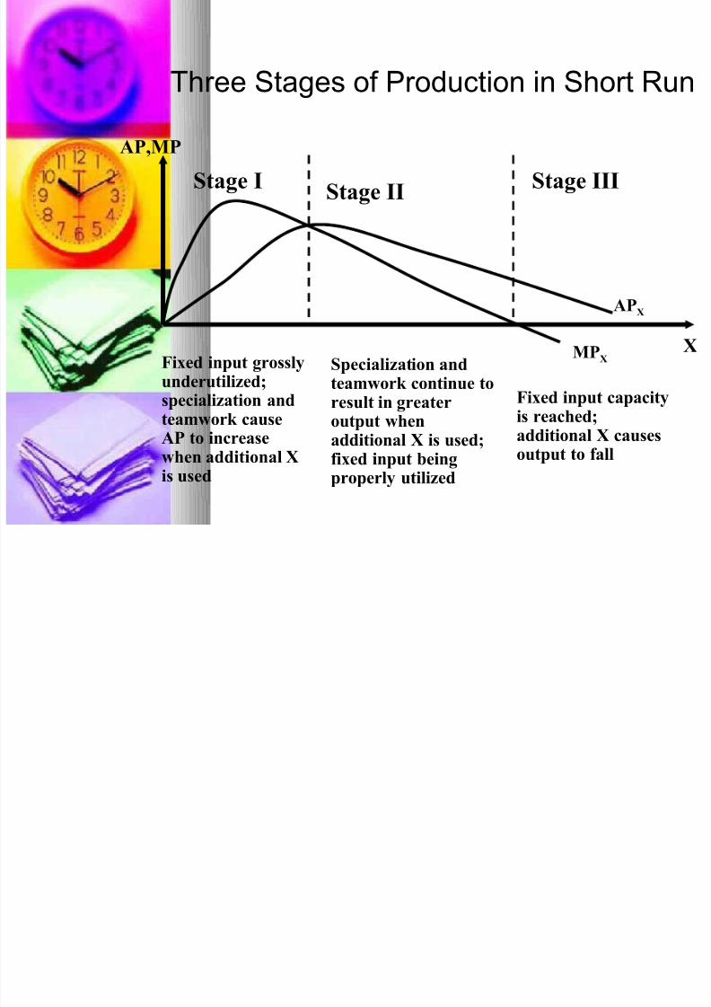
Three Stages of Production in Short Run
AP,MP
X
Stage IStage II
Stage III
APX
MPX
Fixed input grosslyunderutilized;specialization andteamwork causeAP to increasewhen additional Xis used
Specialization andteamwork continue toresult in greateroutput whenadditional X is used;fixed input beingproperly utilized
Fixed input capacityis reached;additional X causesoutput to fall

8/6/2019 Ch-4 Production Theory
http://slidepdf.com/reader/full/ch-4-production-theory 20/45
Stage-1 Stage-2 Stage-3Qu
a
n
ti
t
y
Input-L
L1 L2 L3
TP
MP
AP
Increasing
Return
Decreasing
Return
NegativeReturn
Stage-2 is rational and Stage-1 and 3 are irrational
8/6/2019 Ch-4 Production Theory
http://slidepdf.com/reader/full/ch-4-production-theory 21/45
How to Determine the OptimalInput Usage
We can find the answer to this fromthe concept of derived demand
The firm must know how many units of output it could sell, the price of theproduct, and the monetary costs of employing various amounts of theinput L
Let us for now assume that the firm isoperating in a perfectly competitivemarket for its output and its input

8/6/2019 Ch-4 Production Theory
http://slidepdf.com/reader/full/ch-4-production-theory 22/45

8/6/2019 Ch-4 Production Theory
http://slidepdf.com/reader/full/ch-4-production-theory 23/45
Optimal Decision Rule:
A profit maximizing firm operating in
perfectly competitive output and input
markets will be using optimal amount
of an input at the point at which themonetary value of the input’s marginal
product is equal to the additional cost
of using that input (L)
- in other words, when MRP = MLC
8/6/2019 Ch-4 Production Theory
http://slidepdf.com/reader/full/ch-4-production-theory 24/45
Production in the Long-Run
All inputs are now considered to be
variable (both L and K in our case) How to determine the optimal
combination of inputs?
To illustrate this case we will use productionisoquants.
An isoquant is a curve showing all possible
combinations of inputs physically capable of
producing a given fixed level of output.
It is also known as Iso-Product Curve, Equal
Product Curve, Production Indifference Curve

8/6/2019 Ch-4 Production Theory
http://slidepdf.com/reader/full/ch-4-production-theory 25/45
Example 2 Production Table
Units of K
Employed Output Quantity (Q)
8 37 60 83 96 107 117 127 128
7 42 64 78 90 101 110 119 120
6 37 52 64 73 82 90 97 1045 31 47 58 67 75 82 89 95
4 24 39 52 60 67 73 79 85
3 17 29 41 52 58 64 69 73
2 8 18 29 39 47 52 56 52
1 4 8 14 20 27 24 21 171 2 3 4 5 6 7 8
Units of L
IsoquantUnits of K Employed

8/6/2019 Ch-4 Production Theory
http://slidepdf.com/reader/full/ch-4-production-theory 26/45
An Isoquant
Graph of Isoqua
0
1
2
3
4
5
6
7
1 2 3 4 5 6 7X
Y
8/6/2019 Ch-4 Production Theory
http://slidepdf.com/reader/full/ch-4-production-theory 27/45
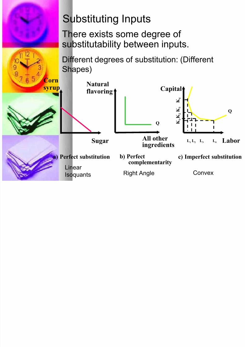
Substituting Inputs
There exists some degree of
substitutability between inputs.
Different degrees of substitution: (Different
Shapes)
Sugar
a) Perfect substitution b) Perfectcomplementarity
All otheringredients
Naturalflavoring
Q
Q
Capital
LaborL1 L2 L3 L4
K1
K2
K3
K4
Corn
syrup
c) Imperfect substitution
Linear
Isoquants Right Angle Convex

8/6/2019 Ch-4 Production Theory
http://slidepdf.com/reader/full/ch-4-production-theory 28/45
Substituting Inputs continued
In case the two inputs are
imperfectly substitutable, theoptimal combination of inputs
depends on the degree of
substitutability and on the relative
prices of the inputs

8/6/2019 Ch-4 Production Theory
http://slidepdf.com/reader/full/ch-4-production-theory 29/45
Substituting Inputs continued
The degree of imperfection insubstitutability is measured with marginalrate of technical substitution (MRTS):
MRTS = ∆ L/∆ K
(in this MRTS some of L is removed from
the production and substituted by K tomaintain the same level of output)

8/6/2019 Ch-4 Production Theory
http://slidepdf.com/reader/full/ch-4-production-theory 30/45
Law of Diminishing Marginal Rateof Technical Substitution:
Table 7.8 Input Combinatio
for Isoquant Q = 52
C ombination L K
A 6 2
B 4 3
C 3 4
D 2 6
E 2 8

8/6/2019 Ch-4 Production Theory
http://slidepdf.com/reader/full/ch-4-production-theory 31/45
Law of Diminishing Marginal Rate of Technical Substitution continued
0
1
2
3
4
5
6
7
2 3 4 6 8X
Y
∆ X = 2∆ Y = -1
∆ X = 1
∆ Y = -1
∆ X = 1
∆Y =- 2
A
BC
DE

8/6/2019 Ch-4 Production Theory
http://slidepdf.com/reader/full/ch-4-production-theory 32/45
MRTS = ∆ L/ ∆ K = - MP L /MP K
Units of K
Employed Output Quantity (Q)
8 37 60 83 96 107 117 127 128
7 42 64 78 90 101 110 119 120
6 37 52 64 73 82 90 97 1045 31 47 58 67 75 82 89 95
4 24 39 52 60 67 73 79 85
3 17 29 41 52 58 64 69 73
2 8 18 29 39 47 52 56 52
1 4 8 14 20 27 24 21 171 2 3 4 5 6 7 8
Units of L
8/6/2019 Ch-4 Production Theory
http://slidepdf.com/reader/full/ch-4-production-theory 33/45
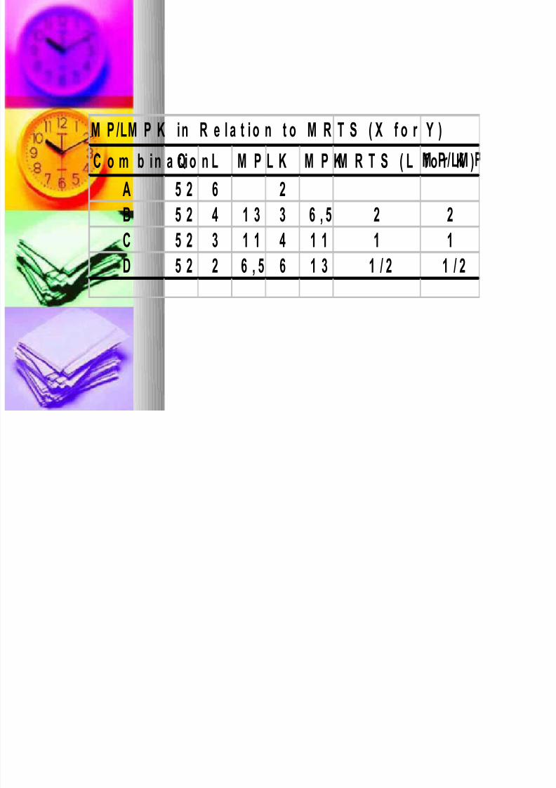
M P L/ M P K in R e l a t i o n t o M R T S ( X f o r Y )
C o m b i n a t i o nQ L M P L K M P KM R T S ( L f o r K )M P L/ M
A 5 2 6 2B 5 2 4 1 3 3 6 , 5 2 2
C 5 2 3 1 1 4 1 1 1 1
D 5 2 2 6 , 5 6 1 3 1 / 2 1 / 2
8/6/2019 Ch-4 Production Theory
http://slidepdf.com/reader/full/ch-4-production-theory 34/45
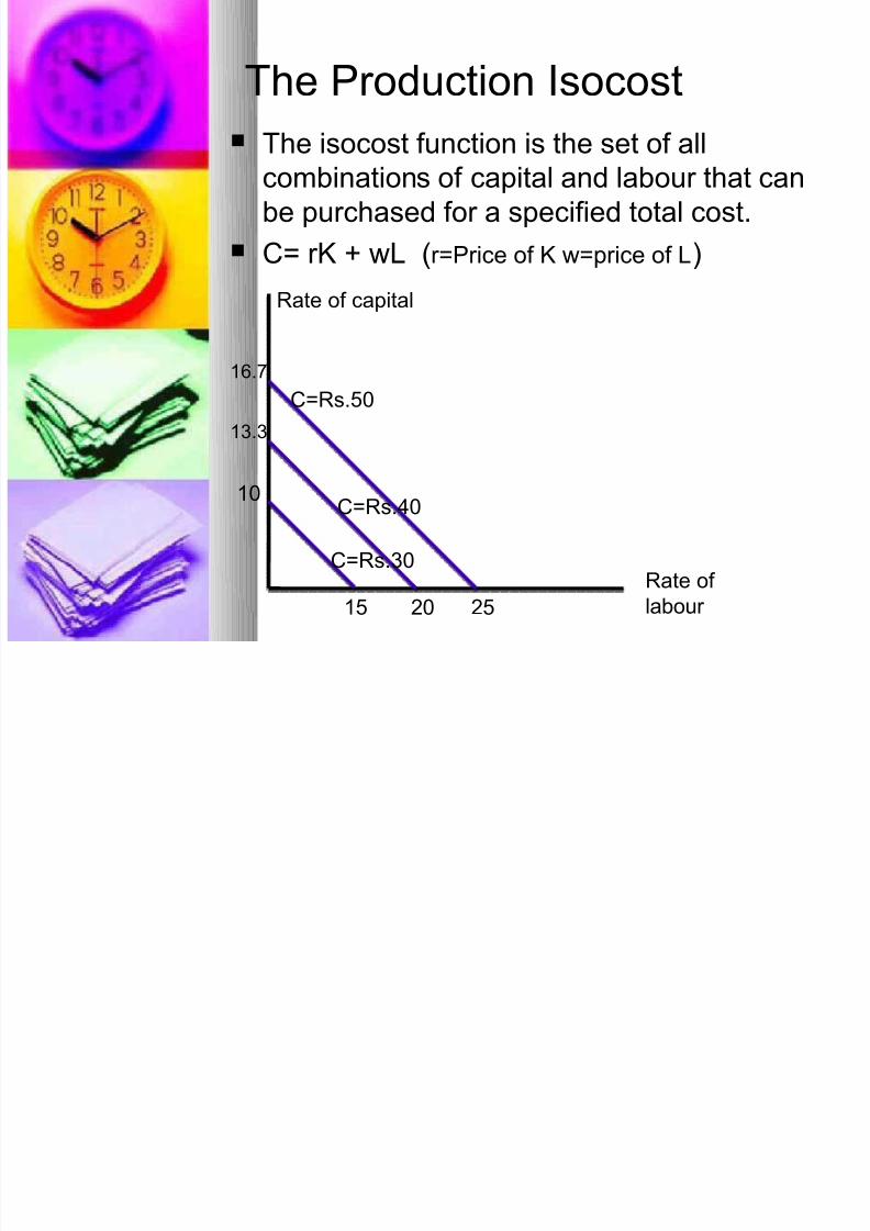
The Production Isocost
The isocost function is the set of allcombinations of capital and labour that can
be purchased for a specified total cost.
C= rK + wL (r=Price of K w=price of L)
Rate of capital
Rate of
labour
16.7
13.3
10
15 20 25
C=Rs.50
C=Rs.40
C=Rs.30
8/6/2019 Ch-4 Production Theory
http://slidepdf.com/reader/full/ch-4-production-theory 35/45
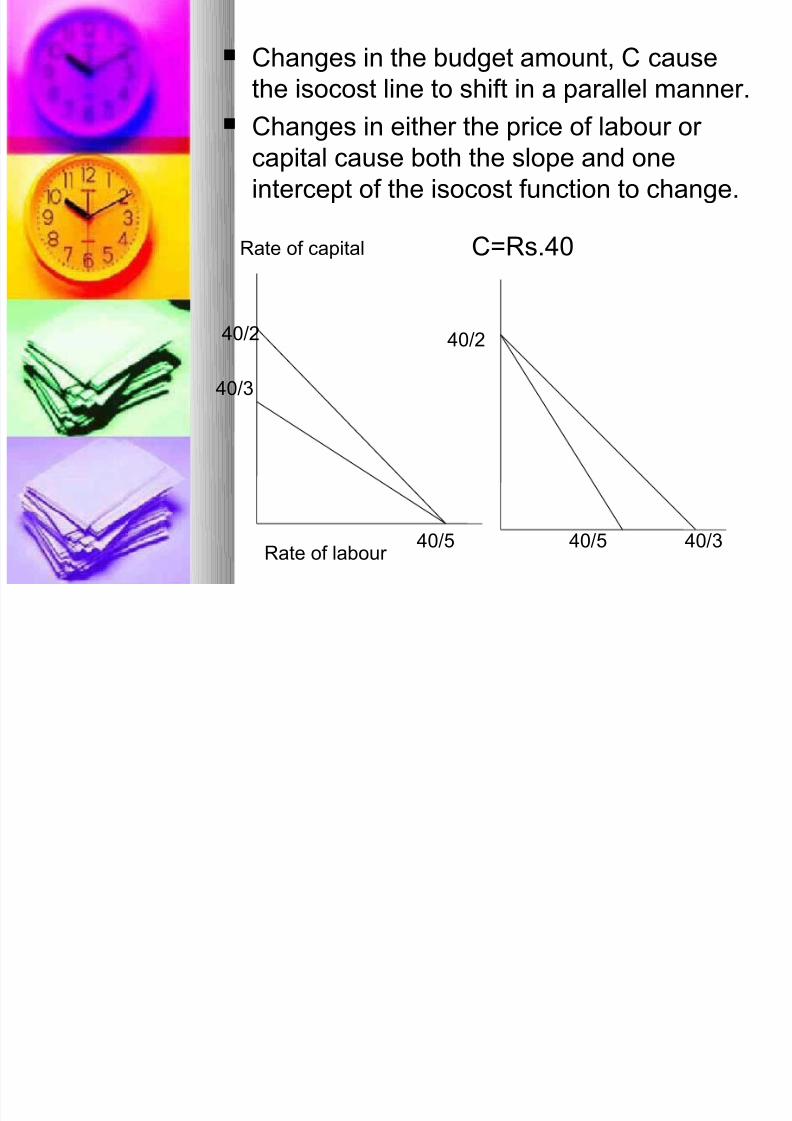
Changes in the budget amount, C cause
the isocost line to shift in a parallel manner.
Changes in either the price of labour or
capital cause both the slope and one
intercept of the isocost function to change.
Rate of capital
Rate of labour
C=Rs.40
40/2
40/3
40/5
40/2
40/5 40/3
8/6/2019 Ch-4 Production Theory
http://slidepdf.com/reader/full/ch-4-production-theory 36/45
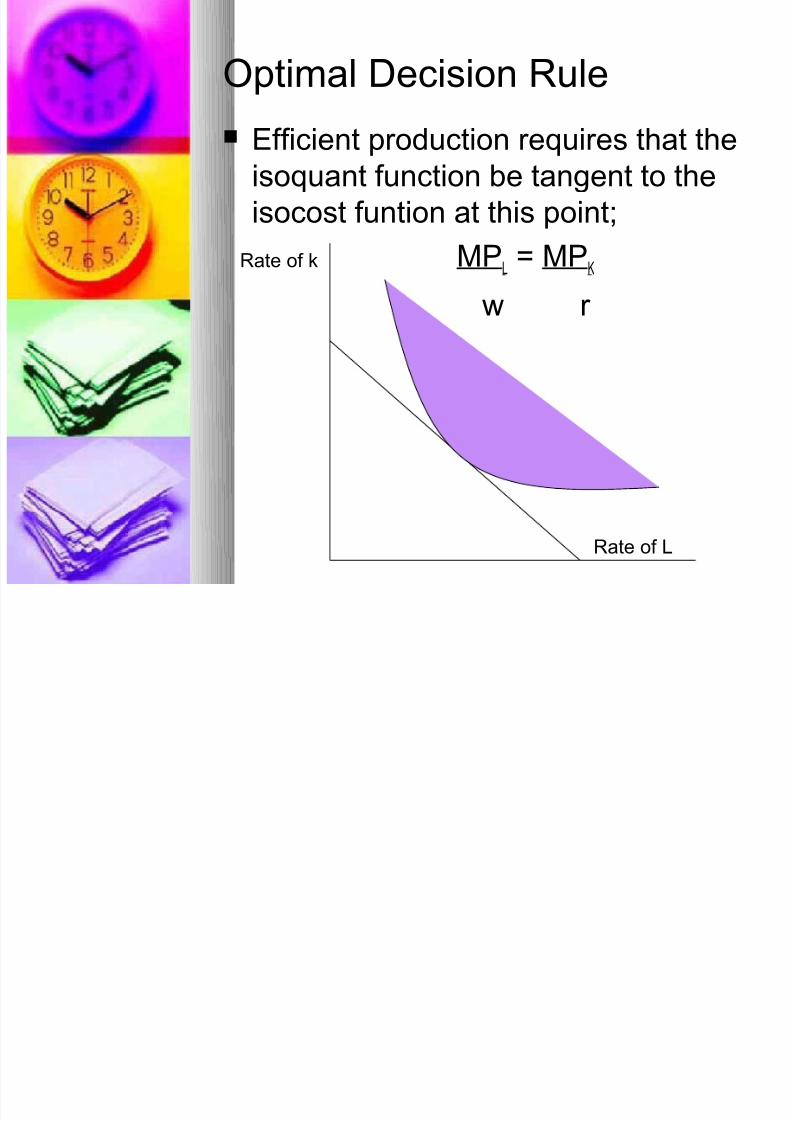
Optimal Decision Rule
Efficient production requires that theisoquant function be tangent to the
isocost funtion at this point;
MPL= MP
K
w r
Rate of L
Rate of k
8/6/2019 Ch-4 Production Theory
http://slidepdf.com/reader/full/ch-4-production-theory 37/45
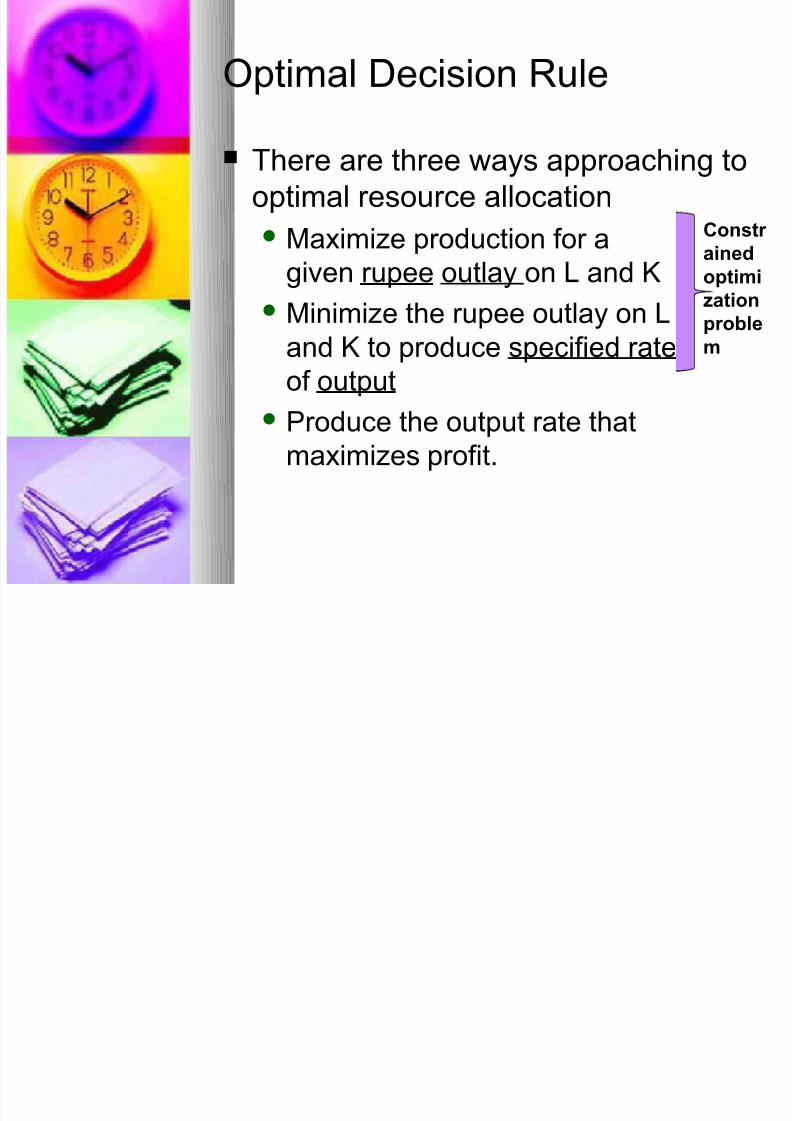
Optimal Decision Rule
There are three ways approaching to
optimal resource allocation
Maximize production for a
given rupee outlay on L and KMinimize the rupee outlay on L
and K to produce specified rate
of output
Produce the output rate thatmaximizes profit.
Constr
ained
optimization
proble
m

8/6/2019 Ch-4 Production Theory
http://slidepdf.com/reader/full/ch-4-production-theory 38/45
Optimal Decision Rule
a
b
c
d
Rs.100
Rs.150
20
10
Rate of K
Rate of L

8/6/2019 Ch-4 Production Theory
http://slidepdf.com/reader/full/ch-4-production-theory 39/45
Optimal decision Rule
If the condition for efficient
production is not met, there is some
way to substitute one input for the
other that will result in an increase atno change in total cost.
Profit maximization requires that
inputs be hired until MRPK=r and
MRPL=w

8/6/2019 Ch-4 Production Theory
http://slidepdf.com/reader/full/ch-4-production-theory 40/45
Economies of Scale
Economies of ScaleA given rate of input of K and L
defines the scale of production.
Change in Scale
Proportionate changes in both inputs
Return to scale
The magnitude of the change in the
rate of output relative to the change inscale.
For eg. P.F. is Q= f(K,L) then
hQ= f( K, L)ƛ ƛh factor change in output when ƛ factor change in both variable
8/6/2019 Ch-4 Production Theory
http://slidepdf.com/reader/full/ch-4-production-theory 41/45

8/6/2019 Ch-4 Production Theory
http://slidepdf.com/reader/full/ch-4-production-theory 42/45
Sources of Economies of
Scale
Reasons for increase
in ROS
Technologies Specialization of
labour
Inventory economy
(increase or replacement)
Reasons for decrease
in ROS
Poor mgt. with thegrowth of the firm.
Transportation cost
Employing large no.
of local labour force.
8/6/2019 Ch-4 Production Theory
http://slidepdf.com/reader/full/ch-4-production-theory 43/45
Economies of Scope
It refers to per-unit cost reductions
that occur when a firm produces two
or more products instead of just one.
Firm can make use of its;Excess capacity
Unique skill or comparative
advantage in marketing to develop
complementary products.
For eg. :- P&G sells all kinds of cleaning
products as well some are complementary such
as laundry det., bleach, and fabric softeners.

8/6/2019 Ch-4 Production Theory
http://slidepdf.com/reader/full/ch-4-production-theory 44/45
Measure of economies of scale
S =TC(QA) + TC(QB) – TC(QA,QB)
TC(QA,QB)
8/6/2019 Ch-4 Production Theory
http://slidepdf.com/reader/full/ch-4-production-theory 45/45
Estimating production function