Ch. 3 - Measurements as Random Variables

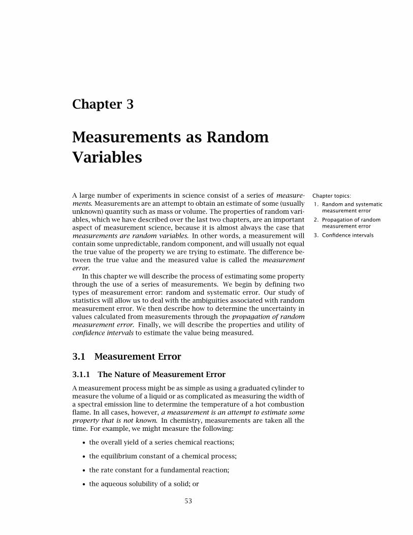
Chapter 3

Measurements as RandomVariables

A large number of experiments in science consist of a series of measure- Chapter topics:

1. Random and systematicmeasurement error

2. Propagation of randommeasurement error

3. Confidence intervals

ments. Measurements are an attempt to obtain an estimate of some (usuallyunknown) quantity such as mass or volume. The properties of random vari-ables, which we have described over the last two chapters, are an importantaspect of measurement science, because it is almost always the case thatmeasurements are random variables. In other words, a measurement willcontain some unpredictable, random component, and will usually not equalthe true value of the property we are trying to estimate. The difference be-tween the true value and the measured value is called the measurementerror.

In this chapter we will describe the process of estimating some propertythrough the use of a series of measurements. We begin by defining twotypes of measurement error: random and systematic error. Our study ofstatistics will allow us to deal with the ambiguities associated with randommeasurement error. We then describe how to determine the uncertainty invalues calculated from measurements through the propagation of randommeasurement error. Finally, we will describe the properties and utility ofconfidence intervals to estimate the value being measured.

3.1 Measurement Error

3.1.1 The Nature of Measurement Error

A measurement process might be as simple as using a graduated cylinder tomeasure the volume of a liquid or as complicated as measuring the width ofa spectral emission line to determine the temperature of a hot combustionflame. In all cases, however, a measurement is an attempt to estimate someproperty that is not known. In chemistry, measurements are taken all thetime. For example, we might measure the following:

• the overall yield of a series chemical reactions;

• the equilibrium constant of a chemical process;

• the rate constant for a fundamental reaction;

• the aqueous solubility of a solid; or

53

54 3. Measurements as Random Variables

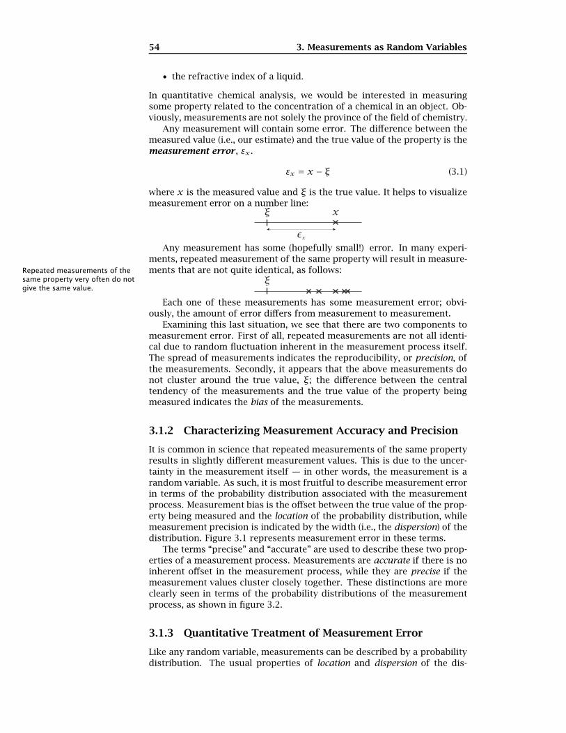
• the refractive index of a liquid.

In quantitative chemical analysis, we would be interested in measuringsome property related to the concentration of a chemical in an object. Ob-viously, measurements are not solely the province of the field of chemistry.

Any measurement will contain some error. The difference between themeasured value (i.e., our estimate) and the true value of the property is themeasurement error , εx .

εx = x − ξ (3.1)

where x is the measured value and ξ is the true value. It helps to visualizemeasurement error on a number line:

ξ x

εxAny measurement has some (hopefully small!) error. In many experi-

ments, repeated measurement of the same property will result in measure-ments that are not quite identical, as follows:Repeated measurements of the

same property very often do notgive the same value.

ξ

Each one of these measurements has some measurement error; obvi-ously, the amount of error differs from measurement to measurement.

Examining this last situation, we see that there are two components tomeasurement error. First of all, repeated measurements are not all identi-cal due to random fluctuation inherent in the measurement process itself.The spread of measurements indicates the reproducibility, or precision, ofthe measurements. Secondly, it appears that the above measurements donot cluster around the true value, ξ; the difference between the centraltendency of the measurements and the true value of the property beingmeasured indicates the bias of the measurements.

3.1.2 Characterizing Measurement Accuracy and Precision

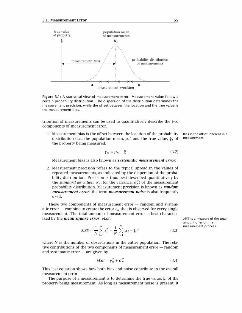
It is common in science that repeated measurements of the same propertyresults in slightly different measurement values. This is due to the uncer-tainty in the measurement itself — in other words, the measurement is arandom variable. As such, it is most fruitful to describe measurement errorin terms of the probability distribution associated with the measurementprocess. Measurement bias is the offset between the true value of the prop-erty being measured and the location of the probability distribution, whilemeasurement precision is indicated by the width (i.e., the dispersion) of thedistribution. Figure 3.1 represents measurement error in these terms.

The terms “precise” and “accurate” are used to describe these two prop-erties of a measurement process. Measurements are accurate if there is noinherent offset in the measurement process, while they are precise if themeasurement values cluster closely together. These distinctions are moreclearly seen in terms of the probability distributions of the measurementprocess, as shown in figure 3.2.

3.1.3 Quantitative Treatment of Measurement Error

Like any random variable, measurements can be described by a probabilitydistribution. The usual properties of location and dispersion of the dis-

3.1. Measurement Error 55

ξ µx

true valueof property

population meanof measurements

probability distributionof measurements

measurement bias

measurement precision

Figure 3.1: A statistical view of measurement error. Measurement value follow acertain probability distribution. The dispersion of the distribution determines themeasurement precision, while the offset between the location and the true value isthe measurement bias.

tribution of measurements can be used to quantitatively describe the twocomponents of measurement error.

1. Measurement bias is the offset between the location of the probability Bias is the offset inherent in ameasurement.distribution (i.e., the population mean, µx) and the true value, ξ, of

the property being measured.

γx = µx − ξ (3.2)

Measurement bias is also known as systematic measurement error.

2. Measurement precision refers to the typical spread in the values ofrepeated measurements, as indicated by the dispersion of the proba-bility distribution. Precision is thus best described quantitatively bythe standard deviation, σx , (or the variance, σ 2

x ) of the measurementprobability distribution. Measurement precision is known as randommeasurement error ; the term measurement noise is also frequentlyused.

These two components of measurement error — random and system-atic error — combine to create the error εx that is observed for every singlemeasurement. The total amount of measurement error is best character-ized by the mean square error , MSE : MSE is a measure of the total

amount of error in ameasurement process.

MSE = 1N

N∑i=1

ε2i =

1N

N∑i=1

(xi − ξ)2 (3.3)

where N is the number of observations in the entire population. The rela-tive contributions of the two components of measurement error — randomand systematic error — are given by

MSE = γ2x + σ 2

x (3.4)

This last equation shows how both bias and noise contribute to the overallmeasurement error.

The purpose of a measurement is to determine the true value, ξ, of theproperty being measurement. As long as measurement noise is present, it


method #1 is moreprecise

than method #2but less accurate

method #1 is moreprecise than method #2

10 20 30 40 50 60 70 80 90

10 20 30 40 50 60 70 80

ξ

ξ

Measurement value

Measurement value

Prob

abil

ity

den

sity

Prob

abil

ity

den

sity

probability distributionfor measurement method #1

measurementmethod #1

probability distributionfor measurement method #2

measurementmethod #2

(a)

(b)

Figure 3.2: Comparison of accuracy and precision of two measurement processeson the basis of the probability distribution of the measurements.


is impossible to know exactly the value of ξ, since random noise is inher-ently unpredictable. However, statistical methods described in this text —confidence intervals, linear regression, hypothesis testing, etc. — allow usto draw conclusions about the value of ξ even with the presence of ran-dom measurement error. Indeed, we might say that the entire purpose ofstatistical data analysis is to allow us to account for the effects of randomfluctuation when drawing conclusions from data.

Measurement bias, however, must be corrected before we can draw mean- Bias must usually be eliminatedfrom the data before statisticalanalysis is performed.

ingful conclusions about our data. We may correct for measurement biasin two ways:

1. We can modify the measurement procedure to eliminate the bias. Inpractice, it is not necessary to completely eliminate the bias; it is suf-ficient to reduce it to levels where the overall measurement error isdominated almost completely by noise. In other words, we reduce thebias, γx , so that

γx � σxEquation 3.4 is relevant in this regard. For example, if we desire that99% of the mean square error, MSE , is due to random error, then weneed to reduce the bias until γ2

x < 0.01σ 2x , or until γx < 0.1σx.

2. Instead of eliminating the bias, we can account for it empirically byapplying a mathematical correction factor to the data. In the simplestcase, we obtain a separate estimate gx of the bias γx and subtract thatestimate from each measurement. For example, in analytical chem-istry it is common to measure the instrument response to the solventin order to correct for inherent instrument offset — the measuredresponse to this “blank” is subtracted from all other measurements.

In some cases, bias correction may not be trivial. For example, it isnot unusual for the measurement bias to exhibit a functional depen-dence on the value of the property being measured: γx = f(x). A biascorrection procedure would be more involved in such a case.

Throughout this text, unless stated otherwise, we assume that measure- Note that statistics can be usedto test for significant bias in aset of measurements, if the truevalue, ξ, of the property beingmeasured is known.

ment bias has been eliminated or corrected in some fashion (i.e., we assumeµx = ξ), so that we will be dealing solely with the effects of random mea-surement error.

Before moving on, let’s do two examples to apply what we’ve learned sofar.

Example 3.1

An overzealous Highway Patrol officer has miscalibrated his radar gunso that there is a bias of +4 mph in the measurements of car speed. If acar is traveling at the speed limit of 65 mph, what is the probability thatthe radar gun will give a measurement greater than 65 mph? Assumethat the measurement precision, as specified by the standard deviationof measurements, is 2.5 mph.

We are given the information that the true car speed — the quantity beingmeasured — is 65 mph: ξ = 65 mph. We need the mean µx and standarddeviation σx of the probability distribution of the radar gun measurements.The question states outright that σx = 2.5, and from eqn. 3.2,

µx = γx + ξ = +4+ 65 = 69 mph


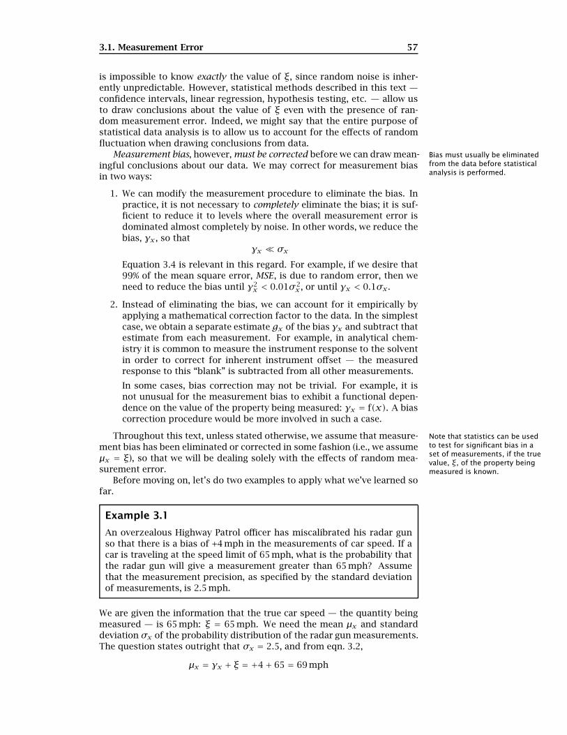
We must find the probability that a single measurement will give a mea-

60 62 64 66 68

µx = 69

ξ = 65

70 72 74 76 78 80

P(x > 65mph)

surement greater than 65 mph, so

P(x > 65 mph) = P(z >

65− µxσx

)= P

(65− 69

2.5

)

= P(z > −1.6)

From eqn. 1.16 on p. 20 (and the z-tables in the appendix)

P(z > −1.6) = 1− P(z > +1.6)= 0.9452

So there is a 94.52% probability that the measured car speed will be greaterthan 65 mph, even though the true car speed is constant at 65 mph. Thisshows the effect of measurement bias: even though the car is traveling atthe speed limit, there is a high probability that the driver will be flaggedfor speeding. If the radar gun exhibited no bias in its measurements, thenQuestion: why would the

probability be 50% if there wereno measurement bias?

there would only be a 50% chance that the measurement would registerabove 65 mph.

Example 3.2

A certain chemist has scrupulously corrected for all systematic errors,and has improved measurement precision as best as she could while at-tempting to weigh a precipitate of silver sulfide. The actual (unknown)mass of the dry precipitate is 122.1 mg. If the relative standard devia-tion (RSD) of the measurement is 2.0%, what is the probability that themeasured mass will have a relative error worse than ±5.0%?

As with so many disciplines in science, one of the most frustrating aspectof statistics is the language barrier. The basic concepts are actually not ter-ribly difficult, but it can be challenging to penetrate the sometimes arcaneterminology that is used. If you are having trouble with a question, oftenthe real barrier is not knowing exactly what information is given or what isasked.

Before we can answer this particular question, we need to recall the defi-nition of relative standard deviation, RSD, from the first chapter (see p. 14):if the value of µx is known, then RSD = σx/µx ; otherwise, it is σx/x (orsometimes σx/x, depending on the context). Knowing the value of the RSDallows us to calculate the standard deviation of the mass measurements,which is needed to solve this problem.

As with the previous example, we need the true value, ξ, and the meanµx and standard deviation σx of the measurement probability distribution.Since measurement bias has been eliminated,

µx = ξ = 122.1 mg

and since RSD = 0.02 (i.e., 2%),

σx = 0.02 · 122.1 = 2.442 mg

We need to find the probability that the relative error is worse than±5.0%. What does this mean? We know that the error εx is simply thedifference between a measurement and the true value: εx = x − ξ. To de-termine the error that corresponds to a relative error of ±5.0%, you should


ask yourself what is meant by ‘relative’ error: relative to what? It mustbe relative to the actual value ξ, which is also the mean of the probabilitydistribution, µx , so that the corresponding error εx is given by:

εx = ±0.05 · 122.1 = ±6.1 mg

So when the question asks “what is the probability that the relative erroris worse than ±5.0%?”, what is really wanted is the probability that themeasurement error will be worse than ±6.1 mg,

P(εx < −6.1)+ P(εx > +6.1) = P(x < 122.1− 6.1)+ P(x > 122.1+ 6.1)= P(x < 116.0)+ P(x > 128.2)

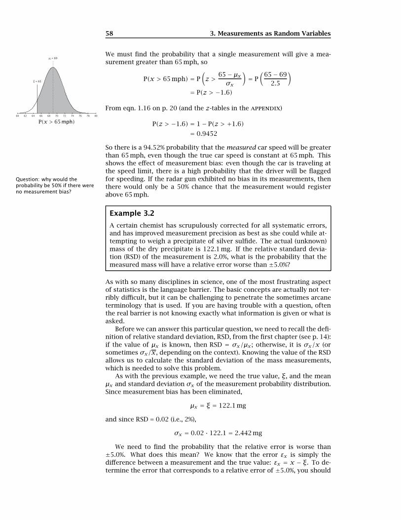
Whew! We’ve finally ‘translated’ the question. We are looking for the sum

110 115 120 125 130 135

116.0

122.1

128.2

P(x < 116.0)+ P(x > 128.2)

of the area in the two tails P(x < 116.0 mg) and P(x > 128.2 mg). Nowthe problem is much easier to solve. If you are familiar with the materialin section 1.3 (hint, hint!), you should be able to understand the followingmanipulations.

P(x < 116.0)+ P(x > 128.2) = P(z <

116.0− 122.12.442

)+ P

(z >

128.2− 122.12.442

)

= P(z < −2.5)+ P(z > +2.5)= 2 · P(z > +2.5)= 0.0124

So, finally, we calculate a 1.24% probability that the relative error is worsethan ±5.0%.

3.1.4 Propagation of Random Measurement Error

Many experiments involve measurements; however, sometimes it is not the ‘Propagation of randommeasurement error’ is oftenshortened to ‘propagation oferror.’

measured value itself that is needed, but some value calculated form themeasurement. For example, we might measure the diameter d of somecoins but we are actually interested in the circumference c = πd of thecoins. The desired property may even required calculations involving two(or more) measurements. If we are interested in the density of an object,we could measure its massm and volume V to calculate the density ρ = m

V .Measurements that contain noise are random variables that must be de- Propagation or error refers to the

determination of the uncertaintyin a value calculated from one ormore random variables.

scribed using probability distributions, sample statistics, etc., because ofthe uncertainty inherent in a random variable. Moreover, any value calcu-lated using one or more random variables is also a random variable. Forexample, if a measured diameter d is a random variable, it has some ‘un-certainty’ associated with it; that uncertainty is the random measurementerror, as quantified by the standard deviation σd. Now, when calculatinga circumference c = πd, that uncertainty necessarily transfers to the cal-culated value — it can’t just disappear! In other words, the calculated cir-cumference c has its own standard deviation σc due to the random mea-surement error in d. We say that the random error has propagated to thecalculated value. We will now describe how to determine the magnitude ofthe propagated error.

Let y be a value calculated from one or more random variables:

y = f(a, b, c, . . . )


where a, b, and c represent random variables. Since y is a function of oneor more random variables, y itself is a random variable whose variance isgiven by

σ 2y =

(∂y∂a

)2

σ 2a +

(∂y∂b

)2

σ 2b +

(∂y∂c

)2

σ 2c + · · · (3.5)

The previous expression depends on the following two assumptions:

1. The errors in the random variables are independent.

2. The calculated value y is a linear function of the variables.

Both of these assumptions are violated routinely. If the first assumptionis violated, knowledge of the measurement error covariance can be used todetermine σy . Violation of the second assumption is not too serious if therelative standard deviations of the measured variables are small (less than10% is pretty safe).

Equation 3.5 is the general expression for propagation of error. How-ever, this expression can be simplified for some common situations. Thesesituations will now be described, and the use of these equations in er-ror propagation calculations will be demonstrated using several examples.Each of the following equations were derived from eqn. 3.5.

Case 1: Addition or Subtraction of Random Variables

When two (or more) random variables are either added or subtracted:

y = a+ bor y = a− b

the variances of the variables are added to determine the variance in thecalculated value.

σ 2y = σ 2

a + σ 2b (3.6a)

σy =√σ 2a + σ 2

b (3.6b)

Remember this rule: variances are additive when two variables are addedor subtracted (as long as the errors are independent). It is a common mis-take to assume that the standard deviations are additive, but they are not:σy ≠ σa + σb.

Case 2: Multiplication or Division of Random Variables

This case is the one that applies to calculating a density of an object frommass and volume measurements. When two random variables are multi-plied or divided,

y = a · by = a

bthen either of the following equations may be used to calculate σy

RSD2y = RSD2

a + RSD2b (3.7a)

σy = y ·√(

σaa

)2

+(σbb

)2

(3.7b)


The first expression is simpler to remember and calculate. In fact, as we willsee, it is simpler to do many error propagation calculations using relativestandard deviation (RSD) values instead of using the standard deviation (σ ).

Case 3: Multiplication or Division of a Random Variable by a Constant

This case is the one that applies to calculating a circumference from a mea-sured diameter, using c = πd. In this last expression, we are not multiply-ing two random variables together, because π is not random. Thus, thiscase is different than the previous one.

When a random variable is multiplied or divided by a constant value, k,

y = k · athe standard deviation of the calculated value y is simply the standard de-viation, σa, of the random variable multiplied by the same constant value.

σy = k · σa (3.8a)

RSDy = RSDa (3.8b)

These equations also apply is a random variable is divided by a constant.For example,

y = yj= k ·y

where k = 1/j. Applying eqn 3.8 gives σy = σa/j.

Case 4: Raising a Random Variable to the kth Power

Let a be a random variable and k be a constant; if we calculate y such that

y = akthen the standard deviation σy can be calculated from

RSDy = |k| · RSDa (3.9a)

σy = |k| ·y · σaa

(3.9b)

It is worth noting that taking the inverse or root of a random variable areboth covered by this case:

y = 1a= a−1 ⇒ RSDy = RSDa

y = √y = y 12 ⇒ RSDy = 1

2RSDa

Case 5: Logarithm/Antilogarithm of a Random Variable

If we calculate the logarithm of a random variable (y = loga), then

σy = RSDaln(10)

σy = 0.434 · RSDa (3.10)

while if we calculate the antilogarithm of a random variable (y = 10a),

σa = RSDyln(10)

RSDy = 2.303 · σa (3.11)


Table 3.1: Useful expressions governing random error propagation in calculations.The simplest expression may be for σy directly, or for RSDy

Case σy RSDyy = a+ by = a− b σ 2

y = σ 2a + σ 2

b

y = a× by = a÷ b RSD2

y = RSD2a + RSD2

b

y = ka(k is a constant)

σy = kσa RSDy = RSDa

y = ak(k is a constant)

RSDy = |k|RSDa

y = loga σy = 0.434 · RSDa

y = 10a RSDy = 2.303σz

Summary and Applications

Table 3.1 summarizes the most useful expressions for propagation of errorcalculations. All of these expressions can be derived from eqn. 3.5. In somecases, the expression for σy is easier to remember or use, while in othersthe calculation of RSDy is simpler.

Being adept at error propagation calculations takes time and practice.First you must master the mechanics: which equation should be used, andwhen? Then you must learn to recognize when an error propagation calcu-lation is appropriate. The first step is really not too difficult to learn; theexamples presented in this section will get you started. The second stepcan be tricky. Real life situations rarely come with a signpost that shouts“error propagation needed here!” Just keep in mind that whenever you per-form a mathematical operation on a measured value, you may need to do arandom error propagation calculation.

With that in mind, let’s do a few examples. The first few will be fairlysimple, and are designed to give you practice in identifying which “case”applies from table 3.1.

Example 3.3

The density of a stainless steel ball bearing is determined in the fol-lowing manner. Its mass is measured in an analytical balance and itsvolume is determined by the displacement of a liquid in a graduatedcylinder. The following measurements were obtained (along with thestandard deviation of these measurements):m = 2.103 g σm = 0.01 gV = 0.34 mL σV = 0.05 mL

Calculate the density and its standard deviation.

First we calculate the density: ρ = 2.1030.34 = 6.185 g/mL. In this calculation,

we divide one measured value by another — since they are both randomvariables, this is Case 2. In order to determine the standard deviation ofthis value, we must use eqn. 3.7.


This problem will be easier if we calculate the relative standard devia-tions of the measurements first.

RSDm = σmm = 0.012.103

= 0.0047551

RSDV = σVV = 0.050.34

= 0.14706

Now we can determine the RSD of the calculated density, and then calculatethe standard deviation of the density:

Note that RSD2m � RSD2

V .RSDρ =√

RSD2m + RSD2

V =√

0.00475512 + 0.147062

= 0.14714

σρ = ρ · RSDρ = 6.185 · 0.14714

= 0.91 g/mL

So the density of the ball bearing is 6.19 g/mL with a standard deviation of0.91 g/mL.

Notice in the last calculation that RSDρ ≈ RSDV . This suggests that if Propagation of error revealswhich measurement contributesthe most to the overalluncertainty.

we wish to decrease the uncertainty in the calculated density we shouldimprove the precision of the volume measurement. Propagation of errorcalculations can be useful in pinpointing the major contributor(s) of uncer-tainty in a value calculated from several measurements.

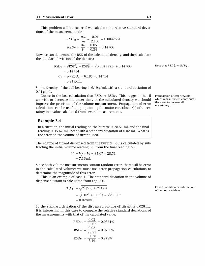
Example 3.4

In a titration, the initial reading on the burette is 28.51 mL and the finalreading is 35.67 mL, both with a standard deviation of 0.02 mL. What isthe error on the volume of titrant used?

The volume of titrant dispensed from the burette, Vt , is calculated by sub-tracting the initial volume reading, Vi, from the final reading, Vf .

Vt = Vf − Vi = 35.67− 28.51

= 7.16 mL

Since both volume measurements contain random error, there will be errorin the calculated volume; we must use error propagation calculations todetermine the magnitude of this error.

This is an example of case 1. The standard deviation in the volume ofdispensed titrant is calculated from eqn. 3.6.

Case 1: addition or subtractionof random variables

σ(Vt) =√σ 2(Vf )+ σ 2(Vi)

=√

0.022 + 0.022) =√

2 · 0.02

= 0.028 mL

So the standard deviation of the dispensed volume of titrant is 0.028 mL.It is interesting in this case to compare the relative standard deviations ofthe measurements with that of the calculated value.

RSDVf =0.02

35.67= 0.0561%

RSDVi =0.02

28.51= 0.0702%

RSDVt =0.0287.16

= 0.279%


Notice that the RSD of the calculated value is quite a bit larger than those ofthe initial measurements. This situation sometimes happens when one ran-dom variable is subtracted from another. In particular, it is always desirableto avoid a situation when the difference between two large measurementsis calculated.

For example, imagine that you want to determine the mass of a feather,and you have the following options:

• Place the feather directly on the scale and measure it

• Measure the mass of an elephant, then place the feather on top of theelephant and mass them both. Calculate the mass of the feather bydifference.

Putting aside the problem of weighing an elephant, which of these methodsThe precision of the calculateddifference between two largemeasurements is often verypoor.

would you prefer? Propagation of error predicts that the precision of thefeather’s mass obtained by the second method would be quite poor becauseyou are taking the different between two large measured values. This is abasic principle in measurement science.

The next example is slightly more complicated in that a value is calcu-lated from a measurement in two steps. The key to applying the simplifyingequations in table 3.1 is that the error should be propagated for each stepof the calculation.

Example 3.5

The solubility of calcium carbonate in pure water is measured to be6.1× 10−8 mol/L at 15 ◦C. This measurement is performed with 7.2%RSD. Calculate the standard deviation of the solubility product, Ksp thatwould be calculated from this measurement.

Calcium carbonate dissolves according toCaCO3 � Ca2+ + CO2−

3The solubility product Ksp is calculated from the molar solubility s as fol-lows:

Ksp =√

2 · s=√

2(6.1× 10−8) = 3.49× 10−4

This calculation actually proceeds in two steps:

Step 1: First multiply the molar solubility by two: y = 2 · sCase 3: multiplication of arandom variable by a constantvalue. This is case 3 — multiplication of a random variable by a constant

value — and so the relative standard deviation remains unchanged:

RSDy = RSDs = 0.072

Step 2: Now we must take the square root: Ksp = √yCase 4: raising a randomvariable to a constant power.

This is case 4, since√y = y 1

2 .

RSDKsp =12

RSDy = 0.5(0.072)

= 0.036

σ(Ksp) = Ksp · RSDKsp = (3.49× 10−4)(0.036)

= 1.256× 10−5


So from the solubility measurement we find that, at this temperature,

Ksp = 3.49× 10−4 and σ(Ksp) = 0.13× 10−4.

In our final example we have a four step calculation using two measuredvalues.

Example 3.6

A cylinder has a measured diameter of 0.25 cm and a length of 250.1 cm.The standard deviation of the first measurement, made with a microme-ter, is 50 microns; the standard deviation of the second measurement is0.3 cm. Calculate the volume from these measurements, and determinethe error in this value.

The volume of the cylinder is calculated using the following equation.

V = πr 2l

Again, we do the random error propagation in steps.

Step 1: Calculate the radius of the circular base: r = d2 Case 3: multiplication of a

random variable by a constant.This is an example of case 3:

r = 0.252

= 0.125 cm

RSDr = RSDd = 0.00500.25

= 0.02

Step 2: Square the radius: y = r2 Case 4: raising a randomvariable to a constant power

This is an example of case 4:

y = 0.1252 = 0.0156 cm2

RSDy = 2 · RSDr = 2(0.02)= 0.04

Step 3: Calculate the area of the circular base: A = π ·y Case 3: multiplication of arandom variable by a constant.

This is case 3 again:

A = π · 0.0156 = 0.0491 cm2

RSDA = RSDy = 0.04

Step 4: Finally, we can calculate the volume: V = A · l Case 2: multiplying two randomvariables together.

This is case 2, since both A and l are random variables.

V = 0.0491 · 250.1 = 12.277 cm3

RSDV =√

RSD2a + RSD2

l =√

0.042 +(

0.3250.1

)2

=√

0.042 + 0.00122 = 0.04001

σV = V · RSDV = 12.277(0.04001)

= 0.4913 cm3


So the volume of the cylinder is 12.28 cm3 with a standard deviationof 0.49 cm3. The major contributor to the uncertainty in the calculatedvolume was the uncertainty in the calculated base circular area, which inturn resulted from random error in the diameter measurement. Thus, todecrease the standard deviation of the calculated volume, the precisionof the diameter measurement must be improved. The error propagationcalculation reveals that improving the precision of the length measurementwould have very little effect on the uncertainty of the calculated volume.

If you wish, you use eqn. 3.5 directly for this calculation. Since

V = πr 2l = π4d2l

and the random variables are the measured values for d and l, applyingeqn. 3.5 yields

σ 2V =

(π2dl)2

σ 2d +

(π4d2)2

σ 2l

= 9645 · 0.0052 + 0.002409 · 0.32

= 0.2411+ 0.0002168 = 0.2413168

σV = 0.4912 cm3

Again it is apparent that the value of σd largely determines the uncer-tainty in the calculated value. Those of you who feel comfortable with par-tial derivatives may prefer to use eqn. 3.5 directly in this manner. In mostcases, it is just as fast (or even faster) to do the propagation calculations ina stepwise manner, using the simplified expressions in table 3.1, and thereis generally less chance of error.

3.2 Using Measurements as Estimates

If the purpose of obtaining measurements is to provide an estimate of anunknown property of some object or system, we must deal with the factthat any estimate will contain a certain amount of measurement error. Evenif all measurement bias has been eliminated, the presence of random errorwill introduce some uncertainty into any single estimate of the property. Asingle measurement value by itself is of limited use in estimating a systemproperty; we also need to indicate somehow the precision, or uncertainty,of this estimate.

A common way to indicate precision is to obtain repeated measure-ments, perhaps under a variety of typical experimental conditions, andthen report both the measurement mean (as the estimate of the systemproperty) and the standard error of the mean (to indicate the estimate’suncertainty). I will now describe how to use a confidence interval to es-timate a property’s true value. The confidence interval is a very usefulestimation method because it accounts for the effects of random error onthe estimate.

3.2.1 Point Estimates and Interval Estimates

Let’s consider an example. The data were originally given in example 2.2on page 44.

3.2. Using Measurements as Estimates 67

Example 3.7

The levels of cadmium, which is about ten times as toxic as lead, in soilis determined by atomic absorption. In five soil samples, the followinglevels were measured:

8.6, 3.6, 6.1, 5.5, 8.4 ppbWhat is the concentration of cadmium in the soil?

The process for the analysis of cadmium in soil would be something likethe following:

1. Collect the samples to be analyzed.

2. Store them in suitable containers and transport them to the labora-tory.

3. Dissolve or extract the soil samples.

4. Use atomic absorption instrument to measure the concentration ofcadmium in the solution.

Performing this entire process repeatedly does not yield the same estimateof cadmium concentration because (i) the cadmium in the soil is not dis-tributed evenly, so that different soil samples will contain different levelsof cadmium; and (ii) even assuming bias has been eliminated, random er-ror will be present in steps 2–4 in the measurement procedure. In orderto account for these effects on our estimate of the “true” concentration ofcadmium in soil, it is necessary to perform measurements repeatedly andthen use sample statistics to provide our estimate.

The important sample statistics for these data are

x = 6.44 ppb

sx = 2.10 ppb

s(x) = sx√5= 0.94 ppb

We use the measurement mean x to estimate the true value ξ of the prop- x �→ µxµx = ξ (no measurement bias)Hence, x �→ ξerty being measured. Of course, the measurement mean actually estimates

the mean µx of the population of measurements, but if we assume no biasin the measurement process (i.e., µx = ξ) then x provides an unbiasedestimate of both µx and ξ.

Sample statistics are sometimes called point estimates of population pa- x is a point estimate of µx.rameters, because they provide a single number representing a “guess” atthe true value of the parameter. Point estimates are simple to interpret,but they have one major disadvantage: they give no indication of the un-certainty of the estimate.

To see why it is important to indicate uncertainty, imagine that the max-imum safe level of cadmium in soil is 8.0 ppb. Can you state with certaintythat the actual concentration of cadmium is below this level? Our bestguess (so far!) of the concentration of cadmium in the soil is 6.44 ppb, butso what? We need an indication of the uncertainty of this estimate.

The standard deviation of the estimate certainly says something aboutits uncertainty. In this case, the standard error of the measurement meanis 0.94 ppb. So what does that tell us? Is the soil cadmium concentrationabove 8.0 ppb?


truevalue

truevalue

pointestimate interval

estimate

Figure 3.3: Comparison of a point estimate and an interval estimate of a populationparameter.

Instead of a single point estimate, it is better by far to provide an inter-val estimate of the true value. An interval estimate is a range of numberswithin which the population parameter is likely to reside. The location andwidth of this range will depend on the point estimate, the standard errorand the number of measurements, so that providing an interval estimateis equivalent to providing all these parameters. Figure 3.3 contrasts thephilosophy of a point estimate and an interval estimate.

An interval estimate always has a confidence level (CL) associated withit. The confidence level is the probability that the interval contains theparameter being estimated. For example, for our cadmium measurements,we might report an interval estimate as follows:

[Cd] = 6.4± 1.5 ppb (90% CL)

The confidence level in this estimate is indicated: there is a 90% proba-bility that the range contains the true cadmium concentration, assuming nomeasurement bias. The interval estimate given here is called a confidenceinterval (CI). It is important to realize that the interval depends on the levelof confidence that is chosen; a higher confidence level (for example, 95%)will give a wider confidence interval.

Confidence intervals are much superior to point estimates as an indi-cation of the values of population parameters. A glance at this confidenceinterval shows that we can be at least “90% confident” that the level of cad-mium in the soil is not 8 ppb or higher; confidence intervals do not requirestatistical expertise to interpret (although some knowledge of statistics isneeded to appreciate them fully). The object of the rest of this chapter is tolearn how to construct and report confidence intervals, and to understandwhy they work.

3.2.2 Confidence Intervals

Introduction

In this section, we will discover how to construct confidence intervals, andexplain why they work. During these explanations, we will sometimes referto a particulate measurement process, described below.


Imagine that we are measuring the concentration of an analyte. Thetrue (but unknown) concentration of the analyte is 50ppm, and the truestandard deviation is 5 ppm. Four measurements of the concentrationare obtained. The following table shows the values of the measurements,as well as other important information.

measurements, ppm: 48.1, 53.3, 59.2, 51.0sample statistics, ppm: x = 53.12, sx = 4.61, s(x) = 2.30true values, ppm: µx = 50, σx = 5, σ(x) = 2.50

The entire process — obtaining a group of four measurements — is re-peated ten more times to generate ten more sample means, each onea mean of mean of four measurements. These data are shown later infig. 3.5.

Example measurement processto illustrate interval estimates.

All measurements are obtainedfrom a population that isnormally distributed with meanµx = 50ppm and standarddeviation σx = 5ppm.

The difference between the sample standard deviation, sx , and the standard s(x) = sx√n

sx �→ σxs(x) �→ σ(x)

error of the mean, s(x), should be emphasized again: sx is an estimate ofσx, which is the standard deviation of the individual measurements, x,while the standard error is an estimate of σ(x), which in this case is thestandard deviation of the mean of 4 measurements.

Prediction Intervals

Before tackling confidence intervals, it is instructive to look at a closely re-lated interval, the prediction interval. The purpose of the prediction inter-val is to indicate the probable range of future values of a random variable.Consider the following problem.

Example 3.8

For a normally distributed variable with a mean of 50 ppm and a stan-dard deviation of 5 ppm, find a range of values that will contain thesample mean of four measurements with a probability of 80%.

Let’s restate the problem. We want to determine x1 and x2 such that

P(x1 < xn < x2) = 1−αwhere n = 4 and α = 0.2, which is the probability that the sample meanfalls outside the values of x1 and x2. Figure 3.4 shows the situation. Notethat we are interested in the probability distribution of the sample mean xnof 4 measurements, not the distribution of the individual measurements, x(which is also shown in the figure as a reference).

We use the z-tables to solve this problem. We must find the z-score zα/2such that

P(x1 < xn < x2) = P(x1 − µxσ(xn)

<x − µxσ(xn)

<x2 − µxσ(xn)

)

= P(−zα/2 < z < zα/2)= 1−α = 0.8

In other words, the value zα/2 is the z-score that gives a right-tail area ofα/2:

P(z > zα/2) = α2


30 35 40 45 50 55 60 65 70

X1 X2

mean of 4 measurements

individual measurements

0.8

Figure 3.4: Figure for example 3.8. We must find the values of x1 and x2 such thatP(x1 < xn < x2) = 1 − α = 0.8. The sampling distribution for the mean of fourmeasurements must be used. The dotted line in the figure shows the distributionof the individual measurements.

For this example, then, we seek z0.1, which is the z-score that gives a right-tail area of 0.1. From the z-tables, the desired value is z0.1 = 1.28. Thismeans that x1 is 1.28 standard deviations below the mean and x2 is 1.28standard deviations above the mean.

−z0.1 = x1 − µxσ(xn)

x1 = µx − z0.1 · σ(xn) = 50− 1.28(

5√4

)

= 46.8 ppm

Likewise,

x1 = µx + z0.1 · σ(xn) = 50+ 1.28(

5√4

)

= 53.2 ppm

Thus our answer: the interval 46.8–53.2 ppm will contain the mean of 4measurements, xn, with 80% probability.

Consider the meaning of the interval found for the last example: thereis a 80% probability that the mean of any four measurements will fall withinthis interval. This range of numbers is called a prediction interval, becauseit can be used to predict where future measurement means will fall.

A prediction interval is a rangeof values that predicts futureobservations with statedprobability.

We calculated our prediction interval by using the z-tables. In other

Important: whenever you usethe z-tables, you are making anassumption of normality. It turnsout that you also make thisassumption when you uset-tables or F -tables, both ofwhich will be introduced later inthis text.

words, we assumed that the mean of four measurements, xn, follows anormal distribution. The central limit theorem provides justification forthis assumption: it states that the probability distribution of the samplemean xn tends to become more normal as the sample size n increases.If the individual measurements x follow a normal distribution — which isoften the situation — then xn follows a normal distribution for any samplesize n. Thus, we will always assume that the sample means are normally


distributed. This assumption is reasonably valid, unless the sample sizeis quite small and the distribution of the individual measurements is quitedifferent than a normal distribution.

A general expression for the prediction interval (PI) with confidence 1−αof a future sample mean x is given by

PI for x = µx ± zα/2 · σ(x) (3.12)

where 1 − α is the probability that the sample mean x lies within the in-terval. In example 3.8 we had α = 0.20 and zα/2 = z0.10 = 1.28. Thus,the prediction interval for the sample mean of four measurements can bewritten as

50.0± 3.2 ppm (80% CL)

meaning that the sample mean would fall within 3.2 ppm of the true mea-surement mean, µx = 50.0 ppm.

Now, the central limit theorem tells us how the standard error of thesample mean, σ(xn), is related to the standard deviation of the individualmeasurements, σx (eqn. 2.9). Using this information, we can also write theprediction interval (eqn. 3.12) as

PI for x = µx ± zα/2 · σx√nwhere n is the number of measurements in the sample mean. It is worthemphasizing the following points about prediction intervals:

• the prediction interval is for the mean of n measurements;

• the width of the prediction interval will depend on both the samplesize n and on the value chosen for α (where the confidence level is1 − α). Increasing sample size narrows the interval, while increasingconfidence levels will widen the prediction interval.

• the prediction interval calculated by eqn. 3.12 assumes that the sam-ple means are normally distributed.

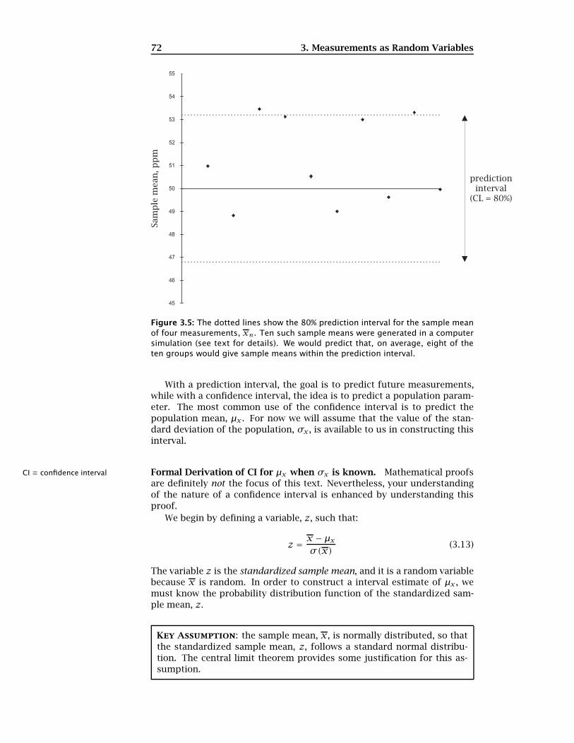
We can illustrate prediction intervals using the measurement processdescribed earlier on page 69. Using a random number generator, 40 mea-surements were generated with µx = 50 and σx = 5. These measurementswere then grouped into 10 samples of four measurements, and the mean xof each sample was calculated, giving a total of ten sample means. Figure3.5 displays the results, along with the 80% prediction interval (as dashedlines). On average — in other words, if this experiment were to be repeatedmany times — eight of the ten sample means should fall within the predic-tion interval.

Interval Estimate of the Population Mean, µx

The step from a prediction interval (PI) to a confidence interval (CI)is a smallone, but an important one. As we will see, the equations used to constructconfidence intervals are almost identical to those used for prediction inter-vals, but the purpose is quite different:

Interval prediction intervals confidence intervals

Purpose

provide a range of valuesthat contain future values ofa variable, with confidencelevel 1−α

provide a range of valuesthat contain the true valueof a population parameter,with confidence level 1−α


45

46

47

48

49

50

51

52

53

54

55

predictioninterval

(CL = 80%)

Sam

ple

mea

n, p

pm

Figure 3.5: The dotted lines show the 80% prediction interval for the sample meanof four measurements, xn. Ten such sample means were generated in a computersimulation (see text for details). We would predict that, on average, eight of theten groups would give sample means within the prediction interval.

With a prediction interval, the goal is to predict future measurements,while with a confidence interval, the idea is to predict a population param-eter. The most common use of the confidence interval is to predict thepopulation mean, µx . For now we will assume that the value of the stan-dard deviation of the population, σx, is available to us in constructing thisinterval.

Formal Derivation of CI for µx when σx is known. Mathematical proofsCI ≡ confidence interval

are definitely not the focus of this text. Nevertheless, your understandingof the nature of a confidence interval is enhanced by understanding thisproof.

We begin by defining a variable, z, such that:

z = x − µxσ(x)

(3.13)

The variable z is the standardized sample mean, and it is a random variablebecause x is random. In order to construct a interval estimate of µx , wemust know the probability distribution function of the standardized sam-ple mean, z.

Key Assumption: the sample mean, x, is normally distributed, so thatthe standardized sample mean, z, follows a standard normal distribu-tion. The central limit theorem provides some justification for this as-sumption.


To construct a confidence interval, we define a value zα/2 such that

P(z > zα/2) = α2which means

P(−zα/2 < z < +zα/2) = 1−αThe key to constructing a confidence interval is the ability to determinethe value zα/2 that satisfies the above expressions. Since we are assumingthat the sample mean x is normally distributed, we may use the z-tables todetermine the value of zα/2 (as we did in example 3.8).

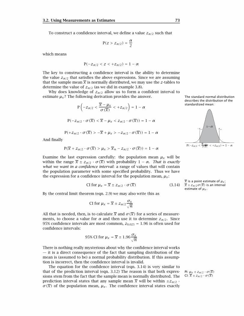
Why does knowledge of zα/2 allow us to form a confident interval toestimate µx? The following derivation provides the answer. The standard normal distribution

describes the distribution of thestandardized mean:

zα/2−zα/2

1 α−

P(−zα/2 < x−µxσ(x) < +zα/2) = 1−α

P(−zα/2 < x − µxσ(x)

< +zα/2)= 1−α

P(−zα/2 · σ(x) < x − µx < zα/2 · σ(x)) = 1−α

P(+zα/2 · σ(x) > −x + µx > −zα/2 · σ(x)) = 1− αAnd finally

P(x + zα/2 · σ(x) > µx > xn − zα/2 · σ(x)) = 1− αExamine the last expression carefully: the population mean µx will bewithin the range x ± zα/2 · σ(x) with probability 1 − α. That is exactlywhat we want in a confidence interval: a range of values that will containthe population parameter with some specified probability. Thus we havethe expression for a confidence interval for the population mean, µx :

x is a point estimate of µx;x ± zα/2σ(x) is an intervalestimate of µx .

CI for µx = x ± zα/2 ·σ(x) (3.14)

By the central limit theorem (eqn. 2.9) we may also write this as

CI for µx = x ± zα/2 σx√nAll that is needed, then, is to calculate x and σ(x) for a series of measure-ments, to choose a value for α and then use it to determine zα/2. Since95% confidence intervals are most common, z0.025 = 1.96 is often used forconfidence intervals:

95% CI for µx = x ± 1.96σx√n

There is nothing really mysterious about why the confidence interval works— it is a direct consequence of the fact that sampling distribution of themean is (assumed to be) a normal probability distribution. If this assump-tion is incorrect, then the confidence interval is invalid.

The equation for the confidence interval (eqn. 3.14) is very similar tothat of the prediction interval (eqn. 3.12) The reason is that both expres- PI: µx ± zα/2 · σ(x)

CI: x ± zα/2 · σ(x)sions stem from the fact that the sample mean is normally distributed. Theprediction interval states that any sample mean x will be within ±zα/2 ·σ(x) of the population mean, µx . The confidence interval states exactly


the same thing; the difference is that where the prediction interval (as de-fined by eqn. 3.12) is concerned with predicting future values of x from aknown value of µx , the confidence interval is used to predict the value ofµx from the known value of x.

We will illustrate confidence intervals by using the measurements men-tioned described at the beginning of this section, on p. 69:

measurements: 48.1, 53.3, 59.2, and 51.9 ppmpopulation parameters: µx = 50 ppm, σx = 5 ppm

Recall that the 80% prediction interval for the sample mean of four mea-surements was earlier (example 3.8) determined to be 50.0±3.2 ppm. If weknow that σx = 5 ppm, then the 80% confidence interval is calculated fromeqn. 3.14:

80% CI for µx = x ± z0.10 ·σ(x)= 53.12± 1.28

(5√4

)

= 53.1± 3.2 ppm

As you can see, the confidence interval does indeed contain the true valueof µx = 50 ppm — although there was a 20% probability that µx was notwithin the interval — and the width of the confidence interval was the sameas the width of the prediction interval, as would be expected.

Figure 3.6 compares the 80% prediction interval and the 80% confidenceintervals from ten sample means generated by computer simulation (asdescribed earlier on page 71). The widths of the prediction and confidenceintervals are the same, so that if the sample mean is within the predictioninterval, then the population mean will be within the confidence interval.

Example 3.9

The concentration of 7 aliquots of a solution of sulfuric acid were mea-sured by titration with sodium hydroxide and found to be 9.8, 10.2, 10.4,9.8, 10.0, 10.2, and 9.6 mM. Assume that the measurements follow a nor-mal probability distribution with a standard deviation of 0.3 mM. Calcu-late a confidence interval for the acid concentration, with a confidencelevel of 95%.

The sample mean, x, and standard error of the mean, σ(x), for the sevenmeasurements can be calculated easily enough.

x = 10.00 mM

σ(x) = σx√n= 0.3√

7= 0.11 mM

For a 95% confidence interval (i.e., α = 0.05) we need the z-score z0.025 =1.96. From eqn. 3.14 we can calculate the confidence interval.

95% CI for µx = 10.00± 1.96 · 0.11

= 10.00± 0.22 mM

We assume no bias in the measurements (γx = 0; ξ = µx) and so theconfidence interval contains the true concentration of sulfuric acid:

[H2SO4] = 10.00± 0.22 mM (95% CL)


45

46

47

48

49

50

51

52

53

54

55

Sam

ple

mea

n, p

pm

Figure 3.6: This is the same data from fig. 3.5: ten sample means were generatedby computer simulation (see text on p. 71 for details). The dotted lines show the80% prediction interval generated by eqn. 3.12, while the error bars on each datapoint show the 80% confidence intervals calculated by eqn. 3.14.

The confidence interval is a powerful method of estimating the truevalue of a measured property. Due to the presence of random measure-ment error, we cannot state with certainty exactly what the concentrationof sulfuric acid is, but we can declare, with stated certainty, that the true(unknown) concentration is within specified range of concentrations. No-tice that there are two significant figures in the second number of the in-terval, and the same number of decimal places in the point estimate (i.e.,the sample mean). It is also perfectly acceptable to use a single significantfigure for the second number: [H2SO4] = 10.0± 0.2 mM.

General Expression: CI for µx when σx is known. The key to the validityof eqn. 3.14 for the confidence interval is that x is a normally distributedvariable. We may generalize eqn. 3.14 for any normally-distributed vari-

a z σ± ·α 2 a/

These twomust match

Confidence Intervals

able, a:

CI for µa = a± zα/2 · σa (3.15)

Applying this general expression to the sample mean (i.e., a = x) giveseqn. 3.14. However, this equation can be used to construct an intervalestimate for the mean µ of any normally distributed variable.

For example, through linear regression we might obtain an estimate b1

for the slope of a line, β1. The point estimate b1 is a sample statistic (i.e., The sample statistic b1 is anestimate of the populationparameter β1:

b1 �→ β1

Linear regression is covered inthe next chapter.

a random variable) and it is often justified to assume that it is normallydistributed. Applying eqn. 3.15 allows us to construct an interval estimateof the true slope β1:

CI for β1 = b1 ± zα/2 ·σ(b1)


A common mistake is to divide the standard deviation by√n, resulting in

the following interval estimate, which is incorrect.

CAREFUL! CI for β1 �= b1 ± zα/2 · σ(b1)√n

The reason we commonly divide by√n is because the central limit theorem

states that the standard error of the sample mean is given by σ(x) = σx√n .

Confidence Interval for µx when σx is not known. The previous methodfor constructing confidence intervals can only be used if the standard de-

When σx is not known — theusual situation — eqn. 3.14cannot be used. viation σx of the entire population of measurements is known. That is

usually not the case; instead, we must use the sample standard deviationsx to provide an estimate of σx. We need to find an expression for an in-terval estimate of µx using the sample statistics x and sx . The steps toderiving such as expression are basically the same as when σx is known(p. 73), so it is helpful to be very comfortable with that material.

To start, we define the variable t as

t = x − µxs(x)

(3.16)

This variable is the studentized sample mean; sometimes called a t-statistic.The studentized mean is similar to the standardized mean (eqn. 3.13), ex-The studentized value of

any random variable x isgiven by x−µxsx

cept σx is not known. The denominator is the sample standard error of themean: s(x) = sx√

n .The ability to construct a confidence interval depends on the ability to

determine the value tα/2 such that

P(t > tα/2) = α2

=+∞∫tα/2

p(t)dt

or, in other words,

P(−tα/2 < t < tα/2) = 1−α

=+tα/2∫−tα/2

p(t)dt

where p(t) is the probability distribution function of the t-statistic. Thisfunction must be known in order to determine tα/2.

Since the studentized sample mean (eqn. 3.16) is very similar to thestandardized sample mean (eqn. 3.13), we might hope that t follows a stan-dard normal distribution, like z. However, even if the sample mean x is nor-mally distribution, t does not follow a normal distribution. That is becausethe standardized mean z is calculated using only one random variable (thesample mean, x) while the studentized mean t is calculated with two vari-ables (x and s(x)). The principle of random error propagation predicts thatthe t-statistic is more variable than the z-statistic, since t is affected by thevariability in both sample statistics.

It turns out that if the sample mean x follows a normal distribution (aspredicted by the central limit theory), then the studentized sample mean t


-4 -3 -2 -1 0 1 2 3 4

ν = 1

ν = 3

ν = 10

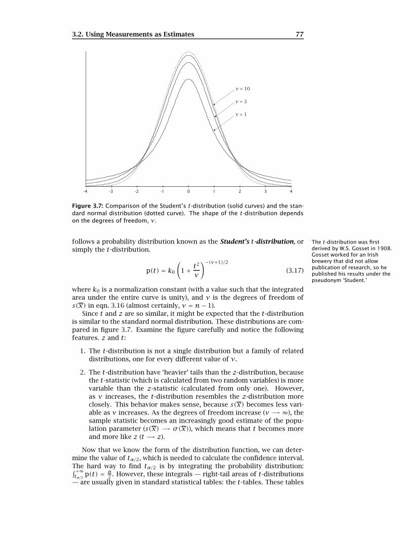
Figure 3.7: Comparison of the Student’s t-distribution (solid curves) and the stan-dard normal distribution (dotted curve). The shape of the t-distribution dependson the degrees of freedom, ν.

follows a probability distribution known as the Student’s t-distribution, orsimply the t-distribution.

p(t) = k0

(1+ t

2

ν

)−(ν+1)/2

(3.17)

where k0 is a normalization constant (with a value such that the integratedarea under the entire curve is unity), and ν is the degrees of freedom ofs(x) in eqn. 3.16 (almost certainly, ν = n− 1).

The t-distribution was firstderived by W.S. Gosset in 1908.Gosset worked for an Irishbrewery that did not allowpublication of research, so hepublished his results under thepseudonym ‘Student.’

Since t and z are so similar, it might be expected that the t-distributionis similar to the standard normal distribution. These distributions are com-pared in figure 3.7. Examine the figure carefully and notice the followingfeatures. z and t:

1. The t-distribution is not a single distribution but a family of relateddistributions, one for every different value of ν.

2. The t-distribution have ‘heavier’ tails than the z-distribution, becausethe t-statistic (which is calculated from two random variables) is morevariable than the z-statistic (calculated from only one). However,as ν increases, the t-distribution resembles the z-distribution moreclosely. This behavior makes sense, because s(x) becomes less vari-able as ν increases. As the degrees of freedom increase (ν �→ ∞), thesample statistic becomes an increasingly good estimate of the popu-lation parameter (s(x) �→ σ(x)), which means that t becomes moreand more like z (t �→ z).

Now that we know the form of the distribution function, we can deter-mine the value of tα/2, which is needed to calculate the confidence interval.The hard way to find tα/2 is by integrating the probability distribution:∫+∞tα/2 p(t) = α

2 . However, these integrals — right-tail areas of t-distributions— are usually given in standard statistical tables: the t-tables. These tables


are structured somewhat differently than the z-tables that given right-tailareas for the standard normal distribution.

The standard normal distribution is a single, unique function (i.e., a nor-mal distribution with µ = 0 and σ = 1), and so a single table can be givento find the value of zα/2 for any value of α. By contrast, the t-distribution isnot a single distribution but a family of related distributions, one for eachdistinct value of ν. For this reason, it is not possible to have a single t-tableto find tα/2 for all possible values of α. Instead, t-tables give the valuesof tα/2 for specific values of α and ν. Inspect the t-table on page A–2 andcompare it to the z-table on page A–1. You must be thoroughly familiarwith the manner in which either table is used.

So now we can derive a confidence interval to estimate the populationmean, µx , from the sample mean, x, and an estimate of its standard error,s(x).

Key Assumption: if the sample mean x is normally distributed, thenthe studentized sample mean, t = x−µx

s(x) follows Student’s t-distribution.The central limit theorem helps justify this assumption.

Once tα/2 can be determined, it is possible to calculate an interval estimate.An expression can be derived as follows.

P(−tα/2 < x − µxs(x)

< +tα/2)= 1−α

P(−tα/2 · s(x) < x − µx < tα/2 · s(x)) = 1− α

P(+tα/2 · s(x) > −x + µx > −tα/2 · s(x)) = 1−αSo that, in the end,

P(x + tα/2 · s(x) > µx > xn − tα/2 · s(x)) = 1− α

This last expression shows that a (1−α) confidence interval for µx — whenσx is not known — is given by

CI for µx = x ± tα/2 · s(x) (3.18)

We can generalize this expression: a confidence interval can be con-structed to estimate the population mean, µa, of a normally distributedvariable from a normally-distributed point estimate a and the sample stan-dard deviation sa of the point estimate:

CI for µa = a± tα/2 · sa (3.19)

It is not hard to see that eqn. 3.18 is a form of this equation with a = x.Let’s use the measurements described on page 69 to show how to con-

struct an interval estimate of µx from a series of measurements.

measurements: 48.1, 53.3, 59.2, and 51.9 ppmsample statistics: x = 53.12 ppm, sx = 4.61 ppm


An 80% confidence interval is calculated as follows.

80% CI for µx = x ± t0.10 · s(x)= 53.12± 1.6377

(4.61√

4

)

= 53.1± 3.8 ppm

Thus, our interval estimate is 53.1 ± 3.8 ppm (80% CL), which does indeedcontain the true concentration of 50 ppm. To determine the value of t0.10

from the t-table, the degrees of freedom, ν, must be known. Since fourmeasurements (n = 4) were used to calculate the standard deviation, sx ,we know that ν = n− 1 = 3.

Figure 3.8 shows 80% confidence intervals calculated using eqn. 3.18.Note that the intervals have different width, since the value of s(x) willchange from sample to sample. In the figure, seven of the ten intervalscontain µx . On average — if the experiment were continued indefinitely –eight out the ten sample means would contain the true mean (solid line),assuming that the sample mean follows a normal probability distribution.

Example 3.10

In the previous example (example 3.9), a 95% confidence interval for theconcentration of sulfuric acid in a solution was calculated, given theinformation that σx = 0.3 mM. Calculate another 95% confidence intervalfor this concentration, this time without assuming any prior knowledgeof σx.

We must calculate the confidence interval entirely from sample statis-tics, since we presumably do not know the value of σx .

x = 10.00 mM

sx = 0.28 mM

s(x) = sx√n= 0.28√

7= 0.11 mM

Since ν = n− 1 = 6,

t0.025 = 2.447

CI for µx = 10.00± 2.447 · 0.11

= 10.00± 0.26 mM (95% CL)

So if we assume no measurement bias, we can say that

[H2SO4] = 10.00± 0.26 mM (95% CL)

Notice that two significant figures were given for the second part of theconfidence interval, and an equivalent number of decimal places were keptin the first part. See section 2.2 for more details.


45

46

47

48

49

50

51

52

53

54

55

Sam

ple

mea

n, p

pm

Figure 3.8: Forty measurements were collected from a normally distributed pop-ulation with µx = 50 and σx = 10 (see p. 69). These values were grouped intoten samples of four measurements each (see text on p. 71). The figure shows theconfidence intervals (calculated from eqn. 3.18) for each of the ten samples.

3.3 Summary and Skills

Measurements usually contain two types of error: random and systematicmeasurement error. The magnitude of the random measurement error, asindicated by the standard deviation of the measurements, is characteristicof measurement precision; the amount of systematic measurement error isthe bias, which indicates the accuracy of the measurements. Bias and stan-dard deviation are statistical concepts that can be related to the probabilitydistribution of the measurements.

Two very important skillsdeveloped in this chapter:

1. Ability to do errorpropagation calculations.

2. Ability to calculateconfidence intervals toestimate µx

If a measurement contains random error, then so too will any value de-rived (i.e., calculated) from that measurement. In some cases, two or moremeasurements are used to calculate the desired result. The procedure todetermine the standard deviation of the derived value is called propagationof (random) error. The error propagation method presented in this chapterassumes that (i) the error of the measurements in the calculation are inde-pendent of one another; and (ii) the calculated value is a linear function ofthe measurements.

Confidence intervals are widely used to estimate population parame-ters. Any confidence interval has an associated confidence level (1−α) thatstates the probability that the population parameter is within the inter-val. In this chapter, methods to calculate confidence intervals for µx weregiven for two situations: (i) the situation when σx is known, and (ii) themore common situation when σx is unknown. Both methods depend onassuming that the sample mean follows a normal probability distribution,an assumption that is somewhat justified by the central limit theorem.

Ch. 3 - Measurements as Random Variables

Documents

Transcript of Ch. 3 - Measurements as Random Variables