Ch. 2: Compression Basics Multimedia...

Ch. 2: Compression Basics Multimedia Systems

Prof. Thinh Nguyen (Based on Prof. Ben Lee’s Slides) Oregon State University

School of Electrical Engineering and

Computer Science

Outline

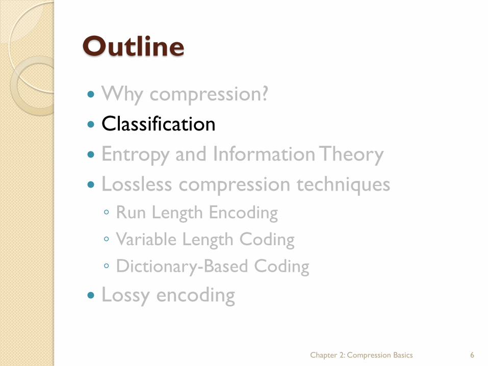
Why compression?

Classification

Entropy and Information Theory

Lossless compression techniques

◦ Run Length Encoding

◦ Variable Length Coding

◦ Dictionary-Based Coding

Lossy encoding

Chapter 2: Compression Basics 2

Why Compression?

100,000

10,000

1,000

100

10

1

1Page 1Page 1Image 1Slide 5 Minute Presentation

Uncompressed Compressed

0.1

0.01

0.001

MB

4.5M

4K

2K

2:1

468K

32K

15:1

1.6M

20:1

60:1

18M

4:1

11M

53M

5:1

342M

70:1

4.9M

1.1G

25:1

46M

620M

37G

Text Fax Computer Image

SVGA

35MM Slide

Audio CD-

Quality Stereo

Videoconf -erence

ISDN Video-Quality

TV-Quality

HDTV High-

Quality

79K

Complexity Example

“NTSC” Quality Computer Display ◦ 640 480 pixel image

◦ 3 bytes per pixel (Red, Green, Blue)

◦ 30 Frames per Second

Bandwidth requirement ◦ 26.4 MB/second

◦ Exceeds bandwidth of almost all disk drives

Storage requirement ◦ CD-ROM would hold 25 seconds worth

◦ 30 minutes would require 46.3 GB

Some form of compression required!


Compression Methods

JPEG for still images

MPEG (1/2/4) for audio/video playback and VoD (retrieval mode applications)

DVI (Digital Visual Interactive) for still and continuous video applications (two modes of compression) ◦ Presentation Level Video (PLV) - high quality

compression, but very slow. Suitable for applications distributed on CD-ROMs

◦ Real-time Video (RTV) - lower quality compression, but fast. Used in video conferencing applications.


Outline

Why compression?

Classification






Lossy encoding


Classification (1)

Compression is used to save storage space, and/or to reduce communications capacity requirements.

Classification ◦ Lossless

No information is lost.

Decompressed data are identical to the original uncompress data.

Essential for text files, databases, binary object files, etc.

◦ Lossy Approximation of the original data.

Better compression ratio than lossless compression.

Tradeoff between compression ratio and fidelity.

e.g., Audio, image, and video.

Classification (2)

Entropy Coding

◦ Lossless encoding

◦ Used regardless of media’s specific characteristics

◦ Data taken as a simple digital sequence

◦ Decompression process regenerates data completely

◦ e.g., run-length coding, Huffman coding, Arithmetic coding

Source Coding

◦ Lossy encoding

◦ Takes into account the semantics of the data

◦ Degree of compression depends on data content

◦ e.g., content prediction technique - DPCM, delta modulation

Hybrid Coding (used by most multimedia systems)

◦ Combine entropy with source encoding

◦ e.g., JPEG, H.263, DVI (RTV & PLV), MPEG-1, MPEG-2, MPEG-4

Symbol Codes

Mapping of letters from one alphabet to another

ASCII codes: computers do not process English

language directly. Instead, English letters are first mapped into bits, then processed by the computer.

Morse codes

Decimal to binary conversion

Process of mapping from letters in one alphabet to letters in another is called coding.

9

Symbol Codes

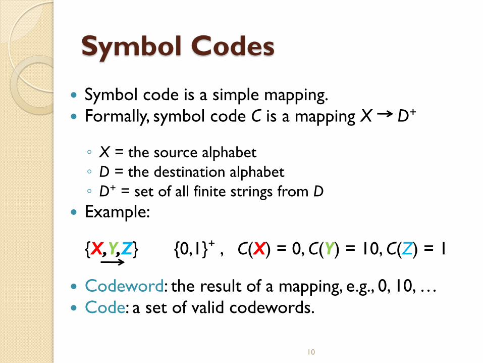
Symbol code is a simple mapping.

Formally, symbol code C is a mapping X D+

◦ X = the source alphabet

◦ D = the destination alphabet

◦ D+ = set of all finite strings from D

Example:

{X,Y,Z} {0,1}+ , C(X) = 0, C(Y) = 10, C(Z) = 1

Codeword: the result of a mapping, e.g., 0, 10, …

Code: a set of valid codewords.

10

Symbol Codes

Extension: C+ is a mapping X+ D+

formed by concatenating C(xi) without punctuation

◦ Example: C(XXYXZY) = 001001110

Non-singular: x1≠x2 → C(x1) ≠C(x2)

Uniquely decodable: C+ is non-singular

◦ That is C+(x+) is unambiguous

11

Prefix Codes

Instantaneous or Prefix code:

◦ No codeword is a prefix of another

Prefix → uniquely decodable → non-

singular

Examples:

C1 C2 C3 C4

W 0 00 0 0

X 11 01 10 01

Y 00 10 110 011

Z 01 11 1110 0111

12

Code Tree

Form a D-ary tree where D = |D|

◦ D branches at each node

◦ Each branch denotes a symbol di in D

◦ Each leaf denotes a source symbol xi in X

◦ C(xi) = concatenation of symbols di along the path from the root to the

leaf that represents xi

◦ Some leaves may be unused

X

W

Y

Z

0

1

1

0 0

0

1

1

C(WWYXZ) =

13

Outline

Why compression?

Classification






Lossy encoding



Entropy and Information

Theory Exploit statistical redundancies in the data to be

compressed.

The average information per symbol in a file, called entropy H, is defined as

where, pi is the probability of the ith distinct symbol.

Entropy is the lower bound for lossless compression, i.e., when the occurring probability of each symbol is fixed, each symbol should be represented with at least with H bits on average.

H = pii

å log2

1

pi

Entropy


The closer the compressed bits per symbol to entropy, the better the compression.

For example, in an image with uniform distribution of gray-level intensity, i.e., pi = 1/256, then the number of bits needed to code each gray level is 8 bits. The entropy of this image is 8. No compression in this case!

We can show that, for an optimal code, the length of a codeword i, Li , satisfies

log2(1/Pi) Li log2 (1/Pi) + 1 Thus, average length of a code word, E[L], satisfies

H(X) E[L] H(X) + 1

Entropy and Compression

In compression, we are interested in constructing an optimum code, i.e., one that gives the minimum average length for the encoded message.

Easy if the probability of occurrence for all the symbols are the same, e.g., last example.

But if symbols have different probability of occurrence…, e.g., Alphabet.

See Huffman and Arithmetic coding.


Outline

Why compression?

Classification






Lossy encoding


Lossless Compression

Techniques Run length encoding (RLE)

Variable Length Coding (VLC)

◦ Huffman encoding

◦ Arithmetic encoding

Dictionary-Based Coding

◦ Lempel-Ziv-Welch (LZW) encoding


Run-Length Encoding

Redundancy is exploited by not transmitting consecutive pixels or character values that are equal.

The value of long runs can be coded once, along with the number of times the value is repeated (length of the run).

Particularly useful for encoding black and white images where the data units would be single bit pixels, e.g., fax.

Methods ◦ Binary RLE

◦ Packbits


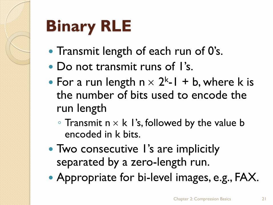
Binary RLE

Transmit length of each run of 0’s.

Do not transmit runs of 1’s.

For a run length n 2k-1 + b, where k is the number of bits used to encode the run length

◦ Transmit n k 1’s, followed by the value b encoded in k bits.

Two consecutive 1’s are implicitly separated by a zero-length run.

Appropriate for bi-level images, e.g., FAX.


Binary RLE


What if stream started with 1? It would start with 0000!

Suppose 4 bits are used to represent the run length

0 . . . 0 1 0 . . . 0 1 1 0 . . . 0 1 0 . . . 0 1 1 0 . . . 0

14 9 20 30 11

1110 1001 0000 1111 0101 1111 1111 0000 0000 1011

All 1’s indicate the next group

is part of the same run

91 bits

40 bits!

Binary RLE Performance

Worst case behavior:

◦ If each transition requires k-bits to encode, and we can have a transition on each bit, k-1 of those bits are wasted. Bandwidth expanded by k times!

Best case behavior:

◦ A sequence of 2k-1 consecutive 0 bits can be represented using k bits. Compression ratio is roughly 2k-1/k e.g., if k = 8, 2k -1 = 255

255:8 » 32:1 compression (lossless).


RLE - Packbits

Used by Apple Macs.

One of the standard forms of compression available in TIFF format (TIFF compression type 32773). ◦ TIFF = Tag Image File format.

Each run is encoded into bytes as follows:


Value0 Valuen-1 ...

Header

Byte Trailer

Bytes

0: Literal run

1: Fill run

Count


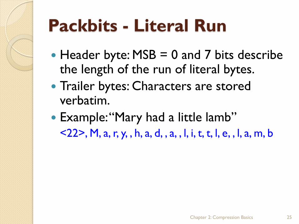
Packbits - Literal Run

Header byte: MSB = 0 and 7 bits describe the length of the run of literal bytes.

Trailer bytes: Characters are stored verbatim.

Example: “Mary had a little lamb”

<22>, M, a, r, y, , h, a, d, , a, , l, i, t, t, l, e, , l, a, m, b


Packbits - Fill Run

Header byte: MSB = 1 and 7 bits describe the length of

the run.

Trailer byte: Byte that should be copied

Example: “AAAABBBBB”

<128+4>A<128+5>B

What about for “ABCCCCCCCCCDEFFFFGGG”?

<129>A<129>B<137>C<129>D<129>E<132>F<131>G

Packbits Performance

Worst case behavior ◦ If entire image is transmitted without

compression, the overhead is a byte (for the header byte) for each 128 bytes.

◦ Alternating runs add more overhead

◦ Poorly designed encoder could do worse.

Best case behavior ◦ If entire image is redundant, then 2 bytes are used

for each 128 consecutive bytes. This provides a compression ratio of 64:1.

Achieves a typical compression ratio of 2:1 to 5:1.


Huffman Coding

Input values are mapped to output values

of varying length, called variable-length

code (VLC):

Most probable inputs are coded with

fewer bits.

No code word can be prefix of another

code word.


Huffman Code Construction

Initialization: Put all nodes (values,

characters, or symbols) in an sorted list.

Repeat until the list has only one node:

◦ Combine the two nodes having the lowest

frequency (probability). Create a parent node

assigning the sum of the children’s

probabilities and insert it in the list.

◦ Assign code 0, 1 to the two branches, and

delete children from the list.


Example of Huffman Coding


P(000) = .5

P(001) = .2

P(010) = .1

P(011) = .08

P(100) = .05

P(101) = .04

P(110) = .03

.5

.2

.1

.08

.07

.05

1.0 0

1

0

1

.5

.3

.2

0

1

.5

.2

.12

.1

.08

0

1

.5

.2

.18

.12

0

1

.5

.5

0

1

000 0

001 11

010 1000

011 1001

100 1011

101 10100

110 10101

Huffman Decoding


P(000) = .5

P(001) = .2

P(010) = .1

P(011) = .08

P(100) = .05

P(101) = .04

P(110) = .03

.5

.2

.1

.08

.07

.05

1.0 0

1

0

1

.5

.3

.2

0

1

.5

.2

.12

.1

.08

0

1

.5

.2

.18

.12

0

1

.5

.5

0

1

000 0

001 11

010 1000

011 1001

100 1011

101 10100

110 10101


Efficiency of Huffman Coding

Entropy H of the previous example:

◦ 0.5 + 0.2 2.32 + 0.1 3.21 + 0.08 3.64 + 0.05 4.32 + 0.04

4.64 + 0.03 5.06 = 2.129

Average number of bits E[L] used to encode a symbol:

◦ 10.5 + 20.2 + 40.1 + 40.08 +4 0.05 + 50.04 + 50.03 =

2.17

Efficiency (2.129/2.17) of this code is 0.981. Very close

to optimum!

If we had simply used 3 bits

◦ 3 (0.5 +0.2 +0.1 +0.08 +0.05 +0.04 +0.03) = 3

So Huffman code is better!


Adaptive Huffman Coding

The previous algorithm requires the statistical knowledge, which is

often not available (e.g., live audio, video)

Even if it’s available, it could be heavy overhead if the coding table is

sent before the data.

◦ This is negligible if the data file is large.

Solution - adjust the Huffman tree on the fly, based on data

previously seen.

Encoder

Initial_code();

while ((c=getc(input))!=eof {

encode (c,output);

update_tree(c);

}

Decoder

Initial_code();

while ((c=decode(input)) !=eof){

putc (c,output);

update_tree(c);

}


Adaptive Huffman Coding

initial_code() assigns symbols with some initially agreed-upon codes without knowing the frequency counts for them.

◦ e.g., ASCII

update_tree() constructs an adaptive Huffman tree.

◦ Huffman tree must maintain its sibling property All nodes (internal and leaf) are arranged in the order of increasing

counts => from left to right, bottom to top.

◦ When swap is necessary, the farthest nodes with count N is swapped with the nodes whose count has just been increased to N+1.


Adaptive Huffman Coding (1)

A B C D 1. w=1 2. w=2 3.w=2 4.w=2

E

8. w=10

9. w=17

5. w=3

7. w=7

6. w=4

A B C D 1. w=2 2. w=2 3.w=2 4.w=2

E

8. w=10

9. w=18

5. w=4

7. w=8

6. w=4

Hit on A

Sibling Property

Increasing order

of weights



2nd hit on A

1 0

0

0 1

1

D B C A 1. w=2 2. w=2 3.w=2 4.w=3

E

8. w=10

9. w=19

5. w=4

7. w=9

6. w=5

1 0

Encoded symbols:

A=011, B=001, C=010

D = 000, E =1

Farthest from A with

count = N = 2

Swap A B C D 1. w=2+1 2. w=2 3.w=2 4.w=2

E

8. w=10

9. w=18

5. w=4

7. w=8

6. w=4



2 more hits on A

Encoded symbols:

A=10, B=1111, C=110

D = 1110, E =0

0 1

1

1

1

0

0

0

D B 1. w=2 2. w=2

E 8. w=10

C 3. w=2

4. w=4 A 5. w=5

6. w=6

7. w=11

9. w=21

D B C A 1. w=2 2. w=2 3.w=2 4.w=3+2

E

8. w=10

9. w=19

5. w=4

7. w=9

6. w=5 Swap

E

8. w=10

9. w=19

7. w=11

6. w=6

Swap

D B 1. w=2 2. w=2

A 5. w=5

C 3. w=2

4. w=4

Adaptive Huffman Coding -

Initialization Initially there is no tree.

Symbols sent for the first time use fixed code: ◦ e.g., ASCII

Any new node spawned from “New”.

Except for the first symbol, any symbol sent afterwards for the first time is preceded by a special symbol “New”. ◦ Count for “New” is always 0.

◦ Code for symbol “New” depends on the location of the node “New” in the tree.

Code for symbol sent for the first time is ◦ code for “New” + fixed code for symbol

All other codes are based on the Huffman tree.



Initialization - Example

New w=0

“A” w=1

• Initially, there is no tree.

• Send AABCDA

• Update tree for “A”

0 1

Suppose we are sending AABCDAD…

◦ Fixed code: A = 00001, B = 00010, C = 00011, D = 00100, …

◦ “New” = 0

Output = 00001 • Decode 00001 = A


• Send AABCDA


Output = 1 • Decode 1 = A


New w=0

“A” w=1

0 1

w=1 w=1

New w=0

“A” w=2

0 1

New w=0

“A” w=2

0 1

w=2 w=2



• Send AABCDA

• Update tree for “B” Output = 0 00010

• Decode 0 00010 = B

• Update tree for “B”

• Send AABCDA

• Update tree for “C” Output = 00 00011

• Decode 00 00011 = C

• Update tree for “C”

“A” w=2

0 1

New w=0

“B” w=1

0 1

w=1

w=3

“A” w=2

0 1

“B” w=1

0 1

New w=0

w=1

w=3

“A” w=2

0 1

“B” w=1

0 1

New w=0

“C” w=1

0 1

w=1

w=2

w=4

“A” w=2

0 1

“B” w=1

0 1

New w=0

“C” w=1

0 1

w=1

w=2

w=4


Initialization - Example • Send AABCDA

• Update tree for “D” Output = 000 00100 • Decode 000 00100 = D

• Update tree for “D”

“A” w=2

0 1

“B” w=1

0 1

“C” w=1

0 1

New w=0

“D” w=1

0 1

w=1

w=2

w=3

w=5

“A” w=2

0 1

“B” w=1

0 1

“C” w=1

0 1

New w=0

“D” w=1

0 1

w=1

w=2

w=3

w=5

“A” w=2

0 1

“B” w=1

0 1

“C” w=1

0 1

New w=0

“D” w=1

0 1

w=1

w=2

w=3

w=5

“A” w=2

0 1

“B” w=1

0 1

“C” w=1

0 1

New w=0

“D” w=1

0 1

w=1

w=2

w=3

w=5

Exchange Exchange



• Send AABCDA

• Update tree for “A” Output = 0 • Decode 0 = A


00001 1 000010 0000011 00000100 0

A A B C D A

“A” w=3

0 1

“B” w=1

0 1

“C” w=1

0 1

New w=0

“D” w=1

0 1

w=1

w=2

w=3

w=6

“A” w=3

0 1

“B” w=1

0 1

“C” w=1

0 1

New w=0

“D” w=1

0 1

w=1

w=2

w=3

w=6

Final transmitted code

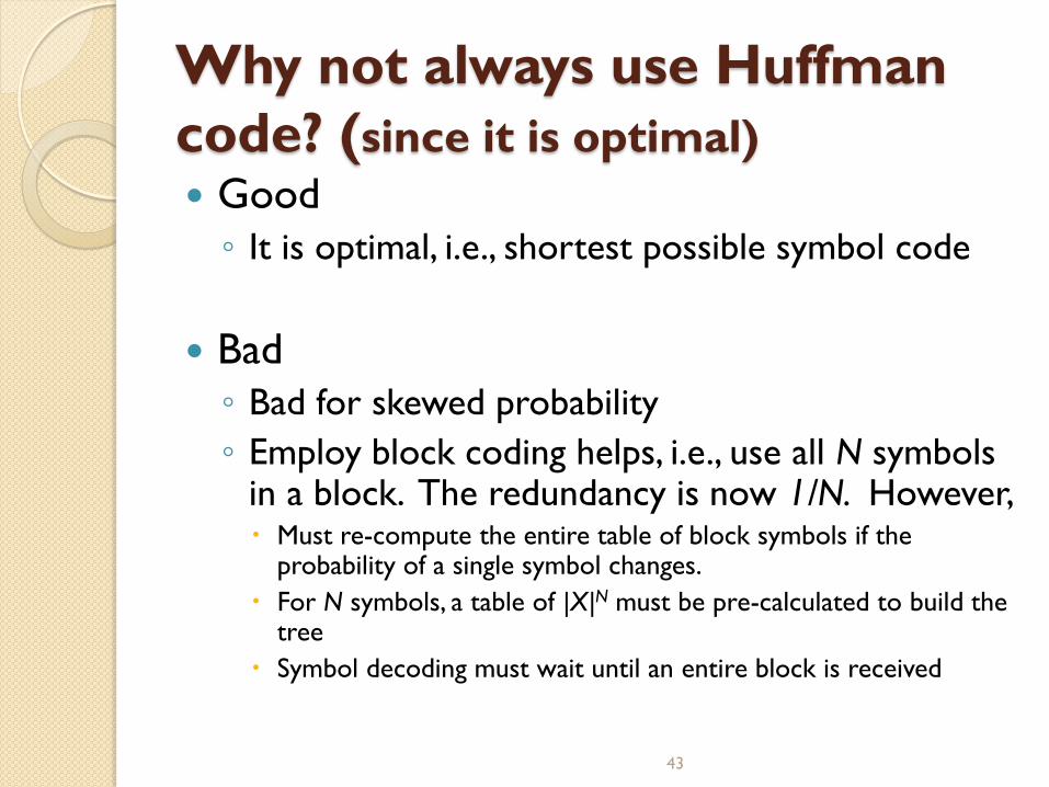
Why not always use Huffman

code? (since it is optimal)

Good

◦ It is optimal, i.e., shortest possible symbol code

Bad

◦ Bad for skewed probability

◦ Employ block coding helps, i.e., use all N symbols in a block. The redundancy is now 1/N. However, Must re-compute the entire table of block symbols if the

probability of a single symbol changes.

For N symbols, a table of |X|N must be pre-calculated to build the tree

Symbol decoding must wait until an entire block is received

43

Arithmetic Coding

Developed by IBM (too bad, they didn’t patent it)

Majority of current compression schemes use it

Good:

◦ No need for pre-calculated tables of big size

◦ Easy to adapt to change in probability

◦ Single symbol can be decoded immediately without waiting for the entire block of symbols to be received.

44

Arithmetic Coding

Each symbol is coded by considering prior data ◦ Relies on the fact that coding efficiency can be

improved when symbols are combined.

◦ Yields a single code word for each string of characters.

◦ Each symbol is a portion of a real number between 0 and 1.

Arithmetic vs. Huffman ◦ Arithmetic encoding does not encode each

symbol separately; Huffman encoding does.

◦ Compression ratios of both are similar.



Arithmetic Coding Example

Example: P(a) = 0.5, P(b) = 0.25, P(c) = 0.25

Coding the sequence “b,a,a,c”

Binary rep. of

final interval

[0.0111, 0.011101)

b a a c


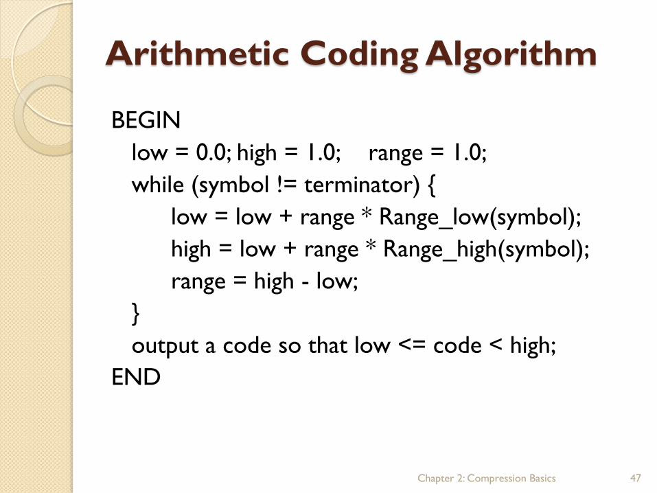
Arithmetic Coding Algorithm

BEGIN

low = 0.0; high = 1.0; range = 1.0;

while (symbol != terminator) {

low = low + range * Range_low(symbol);

high = low + range * Range_high(symbol);

range = high - low;

}

output a code so that low <= code < high;

END


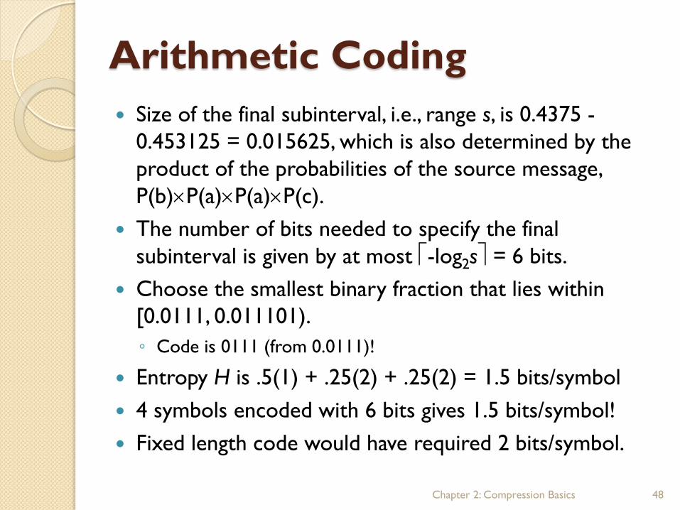
Arithmetic Coding

Size of the final subinterval, i.e., range s, is 0.4375 -

0.453125 = 0.015625, which is also determined by the

product of the probabilities of the source message,

P(b)P(a)P(a)P(c).

The number of bits needed to specify the final

subinterval is given by at most -log2s = 6 bits.

Choose the smallest binary fraction that lies within

[0.0111, 0.011101).

◦ Code is 0111 (from 0.0111)!

Entropy H is .5(1) + .25(2) + .25(2) = 1.5 bits/symbol

4 symbols encoded with 6 bits gives 1.5 bits/symbol!

Fixed length code would have required 2 bits/symbol.


Code Generator for Encoder

BEGIN code = 0; k = 1; while (value(code) < low) { assign 1 to the kth binary fraction bit; if (value(code) > high) replace the kth bit by 0; k = k + 1; } END


For the previous example low = 0.4375 and high = 0.453125. ◦ k = 1: NIL < low, 0.1 (0.5) > high => continue (0.0)

◦ k = 2: 0.0 (0.0) < low, 0.01 (0.25) < high => continue (0.01)



◦ K =5: 0.0111 (0.4375) = low => terminate

Output code is 0111 (from 0.0111)

Code Generator Example


Decoding

BEGIN

get binary code and convert to decimal value = value(code);

do {

find a symbol so that

Range_low(symbol) <= value < Range_high(symbol)

output symbol;

low = Range_low(symbol);

high = Range_high(symbol);

range = high - low;

value = [value - low] / range

}

until symbol is a terminator

END


Decoding Example

.4375 [.4375-.25]/P(b) =.75

a

c 0

0.5

1.0

0.25

b

0.75

= a

a

c 0

0.5

1.0

0.25

b

[.5-.5]/P(a) = 0

= c

a

c

0

0.5

1.0

0.25

b 0.4375

= b

a

c 0

0.5

1.0

0.25

b

[.75-.5]/P(a) =.5

= a

Arithmetic Coding

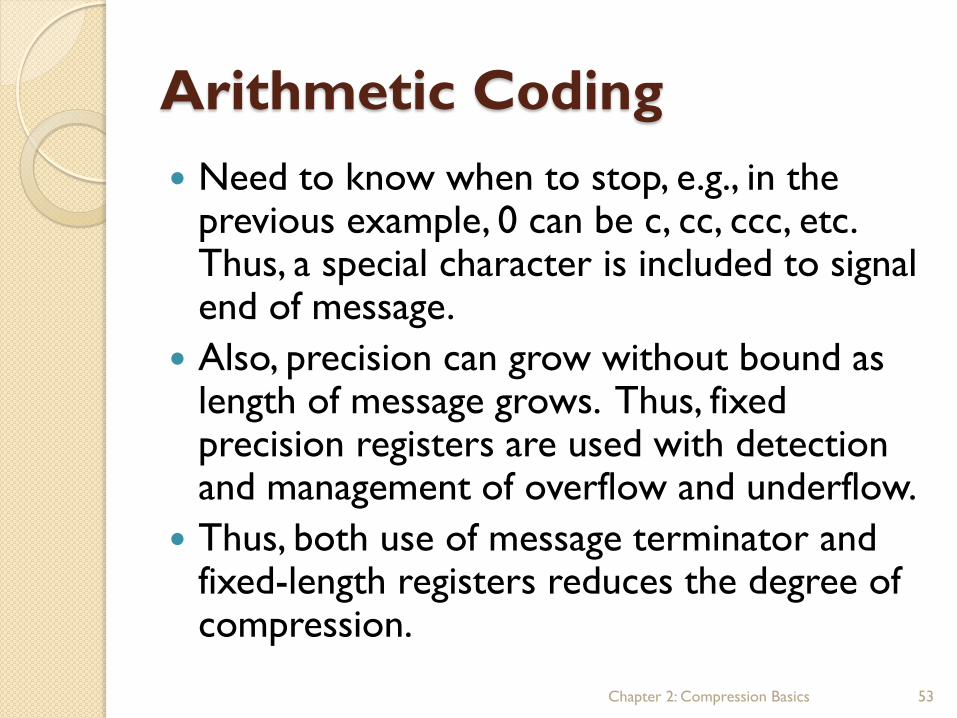
Need to know when to stop, e.g., in the previous example, 0 can be c, cc, ccc, etc. Thus, a special character is included to signal end of message.

Also, precision can grow without bound as length of message grows. Thus, fixed precision registers are used with detection and management of overflow and underflow.

Thus, both use of message terminator and fixed-length registers reduces the degree of compression.


Dictionary Coding

index pattern

1 a

2 b

3 ab

…

n abc

Encoder

codes the

index

Encoder Indices

Decoder

Both encoder and decoder are assumed to have the same dictionary (table)

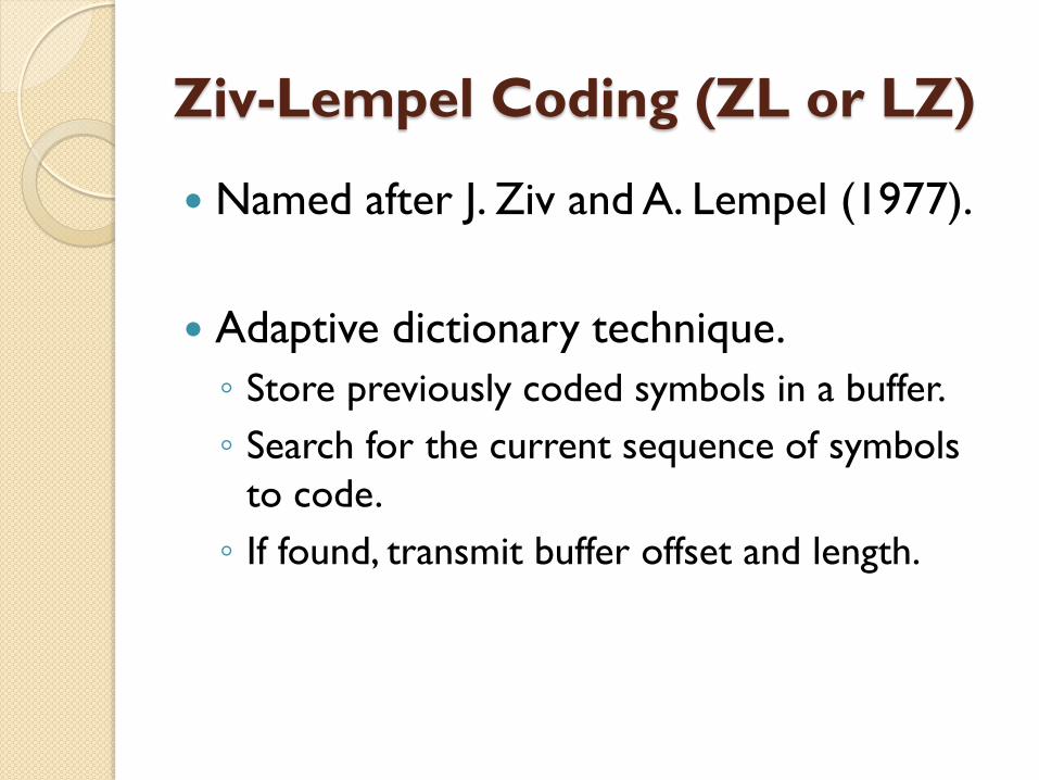
Ziv-Lempel Coding (ZL or LZ)

Named after J. Ziv and A. Lempel (1977).

Adaptive dictionary technique.

◦ Store previously coded symbols in a buffer.

◦ Search for the current sequence of symbols

to code.

◦ If found, transmit buffer offset and length.

LZ77

a b c a b d a c a b d e e e f c

Search buffer Look-ahead buffer

Output triplet <offset, length, next>

1 2 3 4 5 6 7 8

3

8 0 1 3 d 0 e 2 f

2

Transmitted to decoder:

If the size of the search buffer is N and the size of the alphabet is M we need

bits to code a triplet.

Variation: Use a VLC to code the triplets! PKZip, Zip, Lharc,

PNG, gzip, ARJ

Drawbacks of LZ77

Repetetive patterns with a period longer

than the search buffer size are not found.

If the search buffer size is 4, the sequence

a b c d e a b c d e a b c d e a b c d e …

will be expanded, not compressed.

Lempel-Ziv-Welch Coding

Patterns that occur frequently can be substituted by single bytes. ◦ e.g. “begin”, “end”, “if”…

Dynamically builds a dictionary of phrases from the input stream (in addition to the dictionary of 256 ASCII characters).

Checks to see if a phase is recorded in the dictionary ◦ If not, add the phase in the dictionary

◦ Otherwise, output a code for that phrase.

Can be applied to still images, audio, video.

A good choice for compressing text files (used in GIF, .Z, and .gzip compression algorithms).



LZW Compression

s = first input character

while ( not EOF ) {

c = next input character;

if s+c exists in the dictionary

s = s+c;

else {

output the code for s;

add s+c to the dictionary;

s = c;

{

}

output code for s;

Example: Input string is "^WED^WE^WEE^WEB^WET".

19-symbol input has been

reduced to 7-symbol + 5-code output!

s c Output Index Symbol

^ W ^ 256 ^W

W E W 257 WE

E D E 258 ED

D ^ D 259 D^

^ W

^W E 256 260 ^WE

E ^ E 261 E^

^ W

^W E

^WE E 260 262 ^WEE

E ^

E^ W 261 263 E^W

W E

WE B 257 264 WEB

B ^ B 265 B^

^ W

^W E

^WE T 260 266 ^WET

T EOF T


LZW Decompression

s = NIL

While (not EOF) {

k = next input code;

entry = dictionary entry for k;

output entry;

if (s != NIL)

add s + entry[0] to dictionary;

s = entry;

}

Example: Compressed string is

"^WED<256>E<260><261><257>B<260>T".

Decompressor builds its own dictionary,

so only the code needs to be sent!

s k Output Index Symbol

NIL ^ ^

^ W W 256 ^W

W E E 257 WE

E D D 258 ED

D <256> ^W 259 D^

<256> E E 260 ^WE

E <260> ^WE 261 E^

<260> <261> E^ 262 ^WEE

<261> <257> WE 263 E^W

<257> B B 264 WEB

B <260> ^WE 265 B^

260 T T 266 ^WET


LZW Algorithm Details (1)

Example: Input string is

“ABABBABCABBABBAX”.


NIL A A

A B B 256 AB

B <256> AB 257 BA

<256> <257> BA 258 ABB

<257> B B 259 BAB

B C C 260 BC

C <258> ABB 261 CA

<258> <262> ??? 262 ???

… … … … …


A B A 256 AB

B A B 257 BA

A B

AB B 256 258 ABB

B A

BA B 257 259 BAB

B C B 260 BC

C A C 261 CA

A B

AB B

ABB A 258 262 ABBA

A B

AB B

ABB A

ABBA X 262 263 ABBAX

X … X … …

Compressed string is

“AB<256><257>BC<258><262>X…”.

=>

<262> = ABBA =A + BB + A

Whenever encoder encounters Character + String +

Character…, it creates a new code and use it right away

before the decoder has a chance to create it!

Not yet in the dictionary!


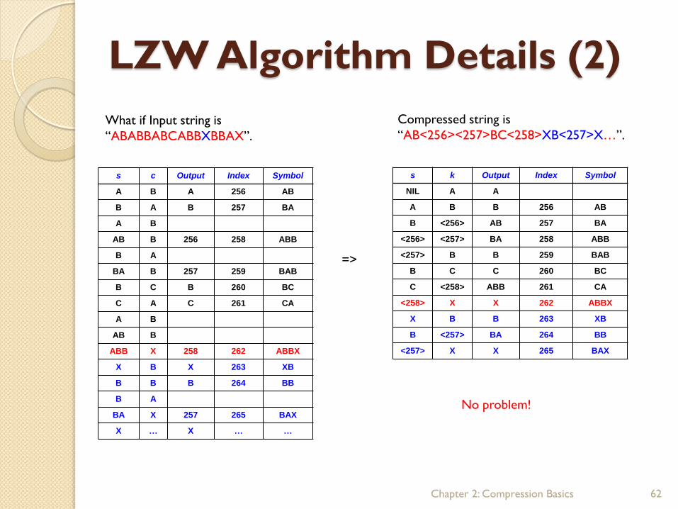
LZW Algorithm Details (2)

What if Input string is

“ABABBABCABBXBBAX”.


NIL A A

A B B 256 AB

B <256> AB 257 BA

<256> <257> BA 258 ABB

<257> B B 259 BAB

B C C 260 BC

C <258> ABB 261 CA

<258> X X 262 ABBX

X B B 263 XB

B <257> BA 264 BB

<257> X X 265 BAX


A B A 256 AB

B A B 257 BA

A B

AB B 256 258 ABB

B A

BA B 257 259 BAB

B C B 260 BC

C A C 261 CA

A B

AB B

ABB X 258 262 ABBX

X B X 263 XB

B B B 264 BB

B A

BA X 257 265 BAX

X … X … …


“AB<256><257>BC<258>XB<257>X…”.

=>

No problem!

Modified LZW Decompression


s = NIL

While (not EOF) {

k = next input code;

entry = dictionary entry for k;

/* Exception Handler */

if (entry == NULL)

entry = s + s[0];

output entry;

if (s != NIL)

add s + entry[0] to

dictionary;

s = entry;

}


A A

A B B 256 AB

B <256> AB 257 BA

<256> <257> BA 258 ABB

<257> B B 259 BAB

B C C 260 BC

C <258> ABB 261 CA

<258> <262> ABBA 262 ABBA

ABBA X X 263 ABBAX


“AB<256><257>BC<258><262>X…”.

ABB + A

s

s[0]; first character of s

Outline

Why compression?

Classification






Lossy encoding


Lossy Encoding

Coding is lossy ◦ Consider sequences of symbols S1, S2, S3, etc., where

values are not zeros but do not vary very much. We calculate difference from previous value => S1, S2-S1, S3-

S2 etc.

e.g., Still image ◦ Calculate difference between nearby pixels or pixel

groups.

◦ Edges characterized by large values, areas with similar luminance and chrominance are characterized by small values.

◦ Zeros can be compressed by run-length encoding and nearby pixels with large values can be encoded as differences.

Ch. 2: Compression Basics Multimedia...

Documents

Transcript of Ch. 2: Compression Basics Multimedia...