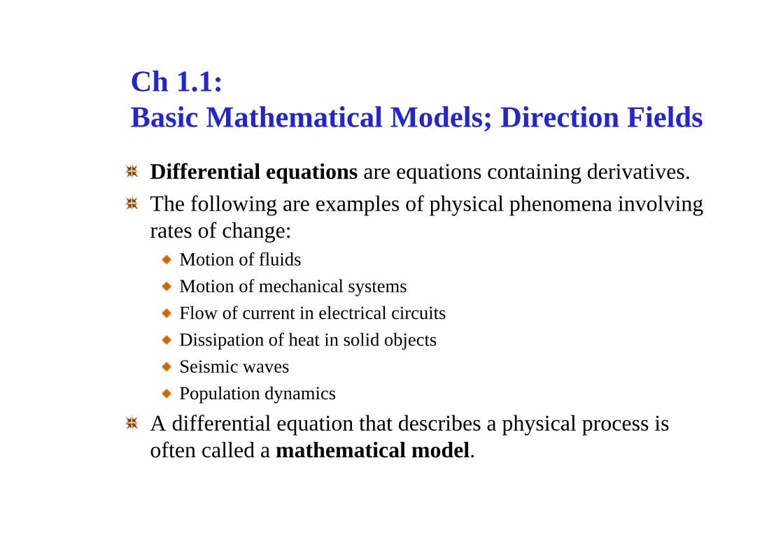
Ch 1.1: Basic Mathematical Models; Direction Fields

Differential equations are equations containing derivatives. The following are examples of physical phenomena involving rates of change:

Motion of fluidsMotion of mechanical systemsFlow of current in electrical circuitsDissipation of heat in solid objects Seismic wavesPopulation dynamics

A differential equation that describes a physical process is often called a mathematical model.

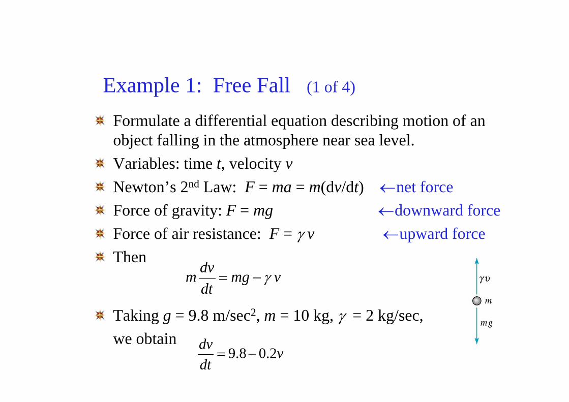
Example 1: Free Fall (1 of 4)

Formulate a differential equation describing motion of an object falling in the atmosphere near sea level. Variables: time t, velocity vNewton’s 2nd Law: F = ma = m(dv/dt) ←net forceForce of gravity: F = mg ←downward forceForce of air resistance: F = γ v ←upward forceThen

Taking g = 9.8 m/sec2, m = 10 kg, γ = 2 kg/sec, we obtain

vmgdtdvm γ−=

vdtdv 2.08.9 −=

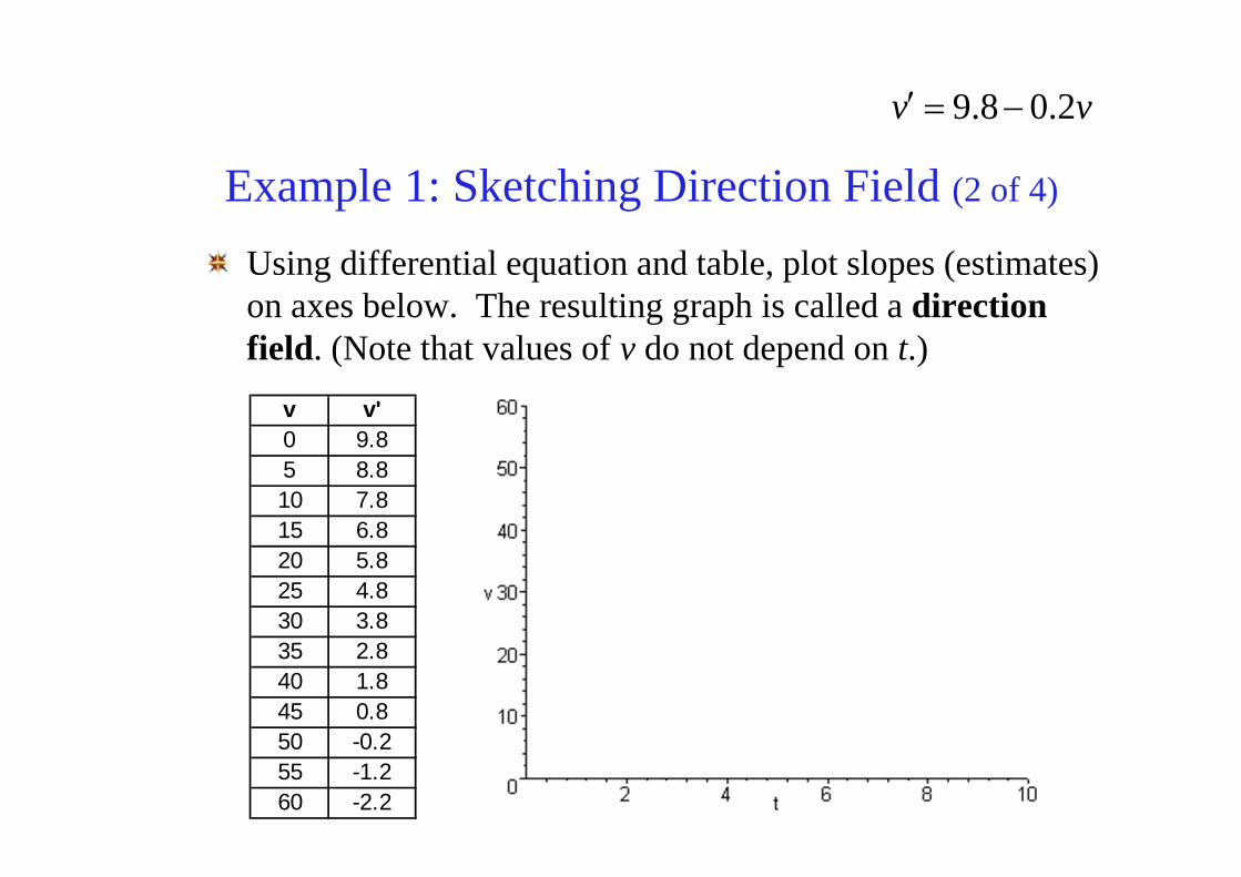
Example 1: Sketching Direction Field (2 of 4)

Using differential equation and table, plot slopes (estimates) on axes below. The resulting graph is called a direction field. (Note that values of v do not depend on t.)

v v'0 9.85 8.810 7.815 6.820 5.825 4.830 3.835 2.840 1.845 0.850 -0.255 -1.260 -2.2

vv 2.08.9 −=′

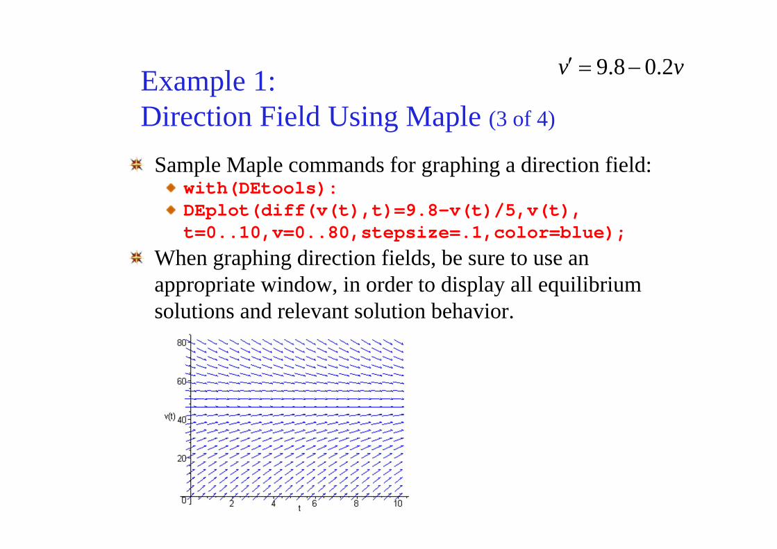
Example 1: Direction Field Using Maple (3 of 4)

Sample Maple commands for graphing a direction field:with(DEtools):DEplot(diff(v(t),t)=9.8-v(t)/5,v(t),t=0..10,v=0..80,stepsize=.1,color=blue);

When graphing direction fields, be sure to use an appropriate window, in order to display all equilibrium solutions and relevant solution behavior.

vv 2.08.9 −=′

Example 1: Direction Field & Equilibrium Solution (4 of 4)

Arrows give tangent lines to solution curves, and indicate where soln is increasing & decreasing (and by how much). Horizontal solution curves are called equilibrium solutions. Use the graph below to solve for equilibrium solution, and then determine analytically by setting v' = 0.

492.08.9

02.08.9:0Set

=⇔

=⇔

=−⇔=′

v

v

vv

vv 2.08.9 −=′

Equilibrium SolutionsIn general, for a differential equation of the form

find equilibrium solutions by setting y' = 0 and solving for y :

Example: Find the equilibrium solutions of the following.

,bayy −=′

abty =)(

)2(352 +=′+=′−=′ yyyyyyy

Example 2: Graphical AnalysisDiscuss solution behavior and dependence on the initial value y(0) for the differential equation below, using the corresponding direction field.

yy −=′ 2

Example 3: Graphical AnalysisDiscuss solution behavior and dependence on the initial value y(0) for the differential equation below, using the corresponding direction field.

35 +=′ yy

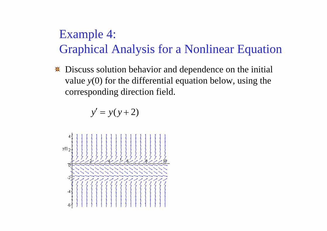
Example 4: Graphical Analysis for a Nonlinear Equation

Discuss solution behavior and dependence on the initial value y(0) for the differential equation below, using the corresponding direction field.

)2( +=′ yyy

Example 5: Mice and Owls (1 of 2)

Consider a mouse population that reproduces at a rate proportional to the current population, with a rate constant equal to 0.5 mice/month (assuming no owls present).When owls are present, they eat the mice. Suppose that the owls eat 15 per day (average). Write a differential equation describing mouse population in the presence of owls. (Assume that there are 30 days in a month.) Solution:

4505.0 −= pdtdp

Example 5: Direction Field (2 of 2)

Discuss solution curve behavior, and find equilibrium soln.

4505.0 −=′ pp

Example 6: Water Pollution (1 of 2)

A pond contains 10,000 gallons of water and an unknown amount of pollution. Water containing 0.02 gram/gal of pollution flows into pond at a rate of 50 gal/min. The mixture flows out at the same rate, so that pond level is constant. Assume pollution is uniformly spread throughout pond.Write a differential equation for the amount of pollution at any given time.Solution (Note: units must match)

yy

yy

005.01min

gal50gal10000

grammin

gal50galgram02.

−=′

⎟⎠⎞

⎜⎝⎛⎟⎟⎠

⎞⎜⎜⎝

⎛−⎟⎠⎞

⎜⎝⎛⎟⎟⎠

⎞⎜⎜⎝

⎛=′

Example 6: Direction Field (2 of 2)

Discuss solution curve behavior, and find equilibrium soln.

yy 005.01−=′

Ch 1.2: Solutions of Some Differential Equations

Recall the free fall and owl/mice differential equations:

These equations have the general form y' = ay - bWe can use methods of calculus to solve differential equations of this form.

4505.0,2.08.9 −=′−=′ ppvv

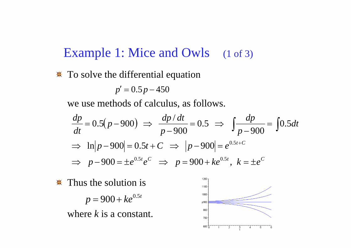
Example 1: Mice and Owls (1 of 3)

To solve the differential equation

we use methods of calculus, as follows.

Thus the solution is

where k is a constant.

4505.0 −=′ pp

( )

CtCt

Ct

ekkepeep

epCtp

dtp

dpp

dtdppdtdp

±=+=⇒±=−⇒

=−⇒+=−⇒

=−

⇒=−

⇒−=

+

∫∫

,900900

9005.0900ln

5.0900

5.0900/9005.0

5.05.0

5.0

tkep 5.0900+=

Example 1: Integral Curves (2 of 3)

Thus we have infinitely many solutions to our equation,

since k is an arbitrary constant. Graphs of solutions (integral curves) for several values of k, and direction field for differential equation, are given below.Choosing k = 0, we obtain the equilibrium solution, while for k ≠ 0, the solutions diverge from equilibrium solution.

,9004505.0 5.0 tkeppp +=⇒−=′

Example 1: Initial Conditions (3 of 3)

A differential equation often has infinitely many solutions. If a point on the solution curve is known, such as an initial condition, then this determines a unique solution.In the mice/owl differential equation, suppose we know that the mice population starts out at 850. Then p(0) = 850, and

t

t

etp

kkep

ketp

5.0

0

5.0

50900)(:Solution50

900850)0(900)(

−=

=−+==

+=

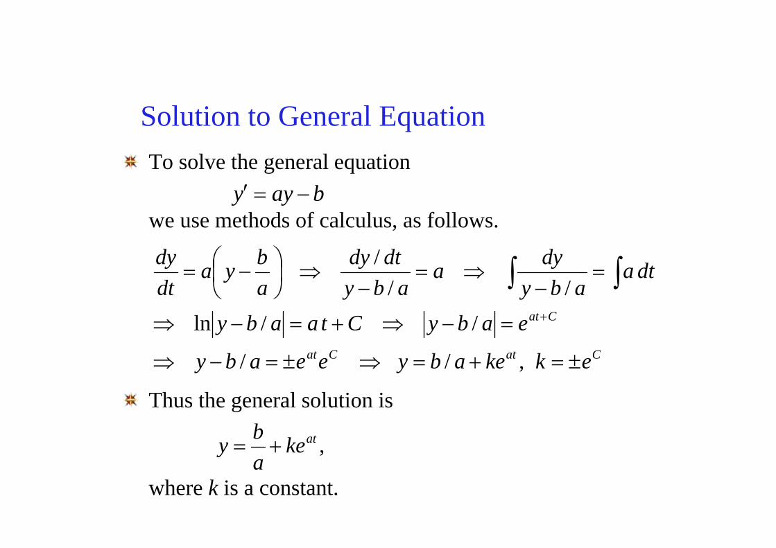
Solution to General EquationTo solve the general equation

we use methods of calculus, as follows.

Thus the general solution is

where k is a constant.

bayy −=′

CatCat

Cat

ekkeabyeeaby

eabyCtaaby

dtaaby

dyaaby

dtdyabya

dtdy

±=+=⇒±=−⇒

=−⇒+=−⇒

=−

⇒=−

⇒⎟⎠⎞

⎜⎝⎛ −=

+

∫∫

,//

//ln//

/

,atkeaby +=

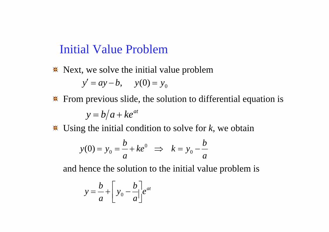
Initial Value ProblemNext, we solve the initial value problem

From previous slide, the solution to differential equation is

Using the initial condition to solve for k, we obtain

and hence the solution to the initial value problem is

ateaby

aby ⎥⎦

⎤⎢⎣⎡ −+= 0

0)0(, yybayy =−=′

atkeaby +=

abykke

abyy −=⇒+== 0

00)0(

Equilibrium SolutionRecall: To find equilibrium solution, set y' = 0 & solve for y:

From previous slide, our solution to initial value problem is:

Note the following solution behavior:If y0 = b/a, then y is constant, with y(t) = b/aIf y0 > b/a and a > 0 , then y increases exponentially without boundIf y0 > b/a and a < 0 , then y decays exponentially to b/a If y0 < b/a and a > 0 , then y decreases exponentially without boundIf y0 < b/a and a < 0 , then y increases asymptotically to b/a

abtybayy

set=⇒=−=′ )(0

ateaby

aby ⎥⎦

⎤⎢⎣⎡ −+= 0

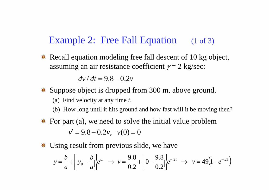
Example 2: Free Fall Equation (1 of 3)

Recall equation modeling free fall descent of 10 kg object, assuming an air resistance coefficient γ = 2 kg/sec:

Suppose object is dropped from 300 m. above ground. (a) Find velocity at any time t. (b) How long until it hits ground and how fast will it be moving then?

For part (a), we need to solve the initial value problem

Using result from previous slide, we have

0)0(,2.08.9 =−=′ vvv

vdtdv 2.08.9/ −=

( )ttat eveveaby

aby 2.2.

0 1492.08.90

2.08.9 −− −=⇒⎥⎦

⎤⎢⎣⎡ −+=⇒⎥⎦

⎤⎢⎣⎡ −+=

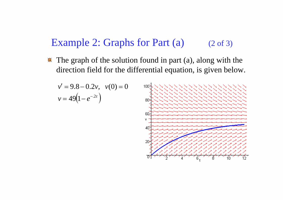
Example 2: Graphs for Part (a) (2 of 3)

The graph of the solution found in part (a), along with the direction field for the differential equation, is given below.

( )tevvvv

2.1490)0(,2.08.9

−−=

=−=′

Example 2Part (b): Time and Speed of Impact (3 of 3)

Next, given that the object is dropped from 300 m. above ground, how long will it take to hit ground, and how fast will it be moving at impact? Solution: Let s(t) = distance object has fallen at time t. It follows from our solution v(t) that

Let T be the time of impact. Then

Using a solver, T ≅ 10.51 sec, hence

24524549)(2450)0(24549)(4949)()(

2.

2.2.

−+=⇒−=⇒=

++=⇒−==′−

−−

t

tt

ettsCsCettsetvts

30024524549)( 2. =−+= − TeTTs

( ) ft/sec01.43149)51.10( )51.10(2.0 ≈−= −ev

Ch 1.3: Classification of Differential Equations

The main purpose of this course is to discuss properties of solutions of differential equations, and to present methods of finding solutions or approximating them.To provide a framework for this discussion, in this section we give several ways of classifying differential equations.

Ordinary Differential EquationsWhen the unknown function depends on a single independent variable, only ordinary derivatives appear in the equation. In this case the equation is said to be an ordinary differential equations (ODE). The equations discussed in the preceding two sections are ordinary differential equations. For example,

4505.0,2.08.9 −=−= pdtdpv

dtdv

Partial Differential EquationsWhen the unknown function depends on several independent variables, partial derivatives appear in the equation. In this case the equation is said to be a partial differential equation (PDE). Examples:

equation) (wave ),(),(

equation)(heat ),(),(

2

2

2

22

2

2

22

ttxu

xtxua

ttxu

xtxu

∂∂

=∂

∂∂

∂=

∂∂α

Systems of Differential EquationsAnother classification of differential equations depends on the number of unknown functions that are involved.If there is a single unknown function to be found, then one equation is sufficient. If there are two or more unknown functions, then a system of equations is required. For example, predator-prey equations have the form

where u(t) and v(t) are the respective populations of prey and predator species. The constants a, c, α, γ depend on the particular species being studied.

Systems of equations are discussed in Chapter 7.

uvcvdtdvuvuadtdu

γα

+−=−=

//

Order of Differential EquationsThe order of a differential equation is the order of the highest derivative that appears in the equation.Examples:

We will be studying differential equations for which the highest derivative can be isolated:

tuu

edt

yddt

ydtyy

yy

yyxx

t

sin

1

02303

22

2

4

4

=+

=+−

=−′+′′=+′

( ))1()( ,,,,,,)( −′′′′′′= nn yyyyytfty K

Linear & Nonlinear Differential EquationsAn ordinary differential equation

is linear if F is linear in the variables

Thus the general linear ODE has the form

Example: Determine whether the equations below are linear or nonlinear.

tuuutuuutdt

ydtdt

ydtyytyeyyy

yyxxyyxx

y

cos)sin()6(sin)5(1)4(

023)3(023)2(03)1(2

2

2

4

4

2

=+=+=+−

=−′+′′=−′+′′=+′

( ) 0,,,,,, )( =′′′′′′ nyyyyytF K

)(,,,,, nyyyyy K′′′′′′

)()()()( )1(1

)(0 tgytaytayta n

nn =+++ − L

Solutions to Differential Equations

A solution φ(t) to an ordinary differential equation

satisfies the equation:

Example: Verify the following solutions of the ODEttyttyttyyy sin2)(,cos)(,sin)(;0 321 =−===+′′

( ))1()( ,,,,,)( −′′′= nn yyyytfty K

( ))1()( ,,,,,)( −′′′= nn tft φφφφφ K

Solutions to Differential Equations

Three important questions in the study of differential equations:

Is there a solution? (Existence)If there is a solution, is it unique? (Uniqueness)If there is a solution, how do we find it?

(Analytical Solution, Numerical Approximation, etc)

Ch 1.4: Historical Remarks

The development of differential equations is a significant part of the general development of mathematics. Isaac Newton (1642-1727) was born in England, and is known for his development of calculus and laws of physics (mechanics), series solution to ODEs, 1665 –1690.Gottfried Leibniz (1646-1716) was born in Leipzig, Germany. He is known for his development of calculus (1684), notation for the derivative (dy/dx), method separation of variables (1691), first order ODE methods (1694).

The Bernoullis

Jakob Bernoulli (1654-1705) & Johann Bernoulli (1667-1748) were both raised in Basel, Switzerland.They used calculus and integrals in the form of differential equations to solve mechanics problems. Daniel Bernoulli (1700-1782), son of Johann, is known for his work on partial differential equations and applications, and Bessel functions.

Leonard Euler (1707-1783)

Leonard Euler (pronounced “oiler”), was raised in Basel, Switzerland, and was the most prolific mathematician of all time. His collected works fill more than 70 volumes.He formulated problems in mechanics into mathematical language and developed methods of solution. “First great work in which analysis is applied to science of movement” (Lagrange).He is known also for his work on exactness of first order ODEs (1734), integrating factors (1734), linear equations with constant coefficients (1743), series solutions to differential equations (1750), numerical procedures (1768), PDEs (1768), and calculus of variations (1768).

Joseph-Louis Lagrange (1736-1813).

Lagrange was raised in Turin, Italy. He was mostly self taught in beginning, and became math professor at age 19. Lagrange most famous for his Analytical Mechanics (1788) work on Newtonian mechanics.Lagrange showed that the general solution of a nth order linear homogenous ODE is a linear combination of nindependent solutions (1762-65). He also gave a complete development of variation of parameters (1774-75), and studied PDEs and calculus of variations.

Pierre-Simon de Laplace (1749-1827).

Laplace was raised in Normandy, France, and was preeminent in celestial mechanics (1799-1825).Laplace’s equation in PDEs is well known, and he studied it extensively in connection with gravitation attraction.The Laplace transform is named after him.

The 1800s

By the end of the 1700s, many elementary methods of solving ordinary differential equations had been discovered.In the 1800s, interest turned to theoretical questions of existence and uniqueness, and series expansions (Ch 5). Partial differential equations also became a focus of study, as their role in mathematical physics became clear. A classification of certain useful functions arose, called Special Functions. This group included Bessel functions, Chebyshev polynomials, Legendre polynomials, Hermite polynomials, Hankel polynomials.

The 1900s – Present

Many differential equations resisted solution by analytical means. By 1900, effective numerical approximation methods existed, but usefulness was limited by hand computation. In the last 50 years, development of computers and robust algorithms have enabled accurate numerical solutions to many differential equations to be generated.Also, creation of geometrical or topological methods of analysis for nonlinear equations occurred which helped foster qualitative understanding of differential equations. Computers and computer graphics have enabled new study of nonlinear differential equations, with topics such as chaos, fractals, etc.