CFD simulations of two-phase flows passing through a...

CFD simulations of two-phase flows passing through a distributor

MARIANNE SJÖSTRAND Department of Applied Mechanics Division of Fluid Dynamics

CHALMERS UNIVERSITY OF TECHNOLOGY Göteborg, Sweden 2008 Master’s Thesis 2008:66

MASTER’S THESIS 2008:66


MARIANNE SJÖSTRAND

Department of Applied Mechanics Division of Fluid Dynamics

CHALMERS UNIVERSITY OF TECHNOLOGY Göteborg, Sweden 2008


MARIANNE SJÖSTRAND ©MARIANNE SJÖSTRAND 2008

Master’s Thesis 2008:66

ISSN 1652-8557

Department of Applied Mechanics Division of Fluid Dynamics

Chalmers University of Technology

SE-412 96 Göteborg Sweden

Telephone: + 46 (0)31-772 1000

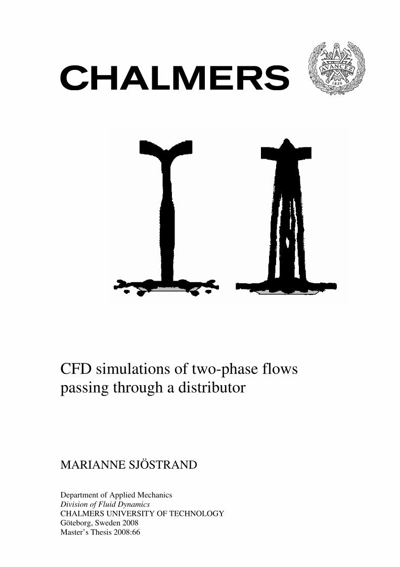
Cover: Overlay of the liquid phase for two different flows passing through a distributor. At left the global flow is lower than at right. Picture obtained for a VOF simulation, see Chapter 3.

Chalmers reproservice Göteborg, Sweden 2008

I

ABSTRACT

This report deals with numerical simulations of two-phase flows in an air/water distributor. The flows are turbulent, unsteady and the liquid phase is under different shapes along the flow: jet, layer, droplets.

The objective of this study is to establish the correct physical models for CFD simulations in order to reproduce experimental data at a wide range of water and air flows.

First, a mesh sensitivity study was made and an optimal cell size was determined for a 2D axisymmetric relevant case.

The influence of different two-phase flow settings has been studied. Nine CFD simulations on a simplified 3D geometry have been performed, with a fine mesh. Two flows having different associated Weber numbers (<1 and ~30) have been considered. VOF simulations have been compared with Euler/Euler simulations. Euler/Euler simulations have been performed with two different liquid phase characteristic lengths. The differences in the results are not significant but they are clearer for the case where the Weber number is less than one, i.e. the case where the surface tension effects are stronger.

Finally, entire simulations of the flow have been performed for eight different operating conditions among the experimental data and using an Euler/Euler model. The Euler/Euler model is more adapted for the simulation of a dispersed flow. The simulated cases can be classified as follow:

Weber ~ 30

Weber ~ 10

Weber < 3

The post-treatment of simulations results consists in comparing the simulations’ water distribution downstream the distributor with the experimental data. This comparison shows that for Weber ~ 30 the CFD simulations are predictive.

Key words: VOF, Euler/Euler, two-phase flows, CFD, Weber number

CHALMERS, Applied Mechanics, Master’s Thesis 2008:66 III

Contents

ABSTRACT I

CONTENTS III

PREFACE V

ACKNOWLEDGEMENTS V

NOTATIONS VII

USEFUL VOCABULARY IX

1 INTRODUCTION 1

1.1 Background 1

1.2 Problem definition and purpose 1

1.3 Structure of the report 2

2 PRESENTATION OF THE FLOWS 3

2.1 The distributor 3

2.2 The whole domain 3

2.3 Material properties 5

2.4 Inlet volume flow rates 5

2.5 Inlet Reynolds Numbers 6

2.6 Weber number calculation at the ejection 6

2.7 Experimental observations of the flow 7

2.8 Time scales of the simulations 8

3 CFD SETTINGS TO RESOLVE AN UNSTEADY, TWO-PHASE, TURBULENT FLOW 11

3.1 The multiphase models 11 3.1.1 Basic notions in two-phase flows 11 3.1.2 The VOF model 12 3.1.3 The Euler/Euler model 13

3.2 The RNG k-ε turbulence model 16 3.2.1 The Reynolds Averaged Navier Stokes (RANS) approach 16 3.2.2 The Boussinesq Approach 17 3.2.3 RNG k-ε model 17 3.2.4 The wall effect treatment 19

3.3 The transient solver 20 3.3.1 Presentation of the resolution schemes 20 3.3.2 Variable time step for VOF simulations 20 3.3.3 Adaptive time stepping for Euler/Euler simulations 21

CHALMERS, Applied Mechanics, Master’s Thesis 2008:66 IV

4 PRELIMINARY STUDIES 23

4.1 Estimation of the optimized grid: mono-phase 2D simulations 23 4.1.1 Purposes of the study 23 4.1.2 Approach 23 4.1.3 Main results 24

4.2 Comparison of VOF simulations and Euler/Euler simulations 26 4.2.1 Purposes of the study 26 4.2.2 Overlay and reference surfaces 27 4.2.3 Estimation of the establishment flow time 28 4.2.4 Qualitative results for the high air flow case “V1 v9” 29 4.2.5 Qualitative results for the air flow case “V1 v3” 30 4.2.6 Post-treatment to compare the VOF and the Euler/Euler cases 32 4.2.7 Quantitative results of the case “V1 v9” simulations 33 4.2.8 Quantitative results of the case “V1 v3” simulations 34 4.2.9 Conclusions of the quarter of geometry study 35

5 SIMULATIONS OF THE ENTIRE GEOMETRY 37

5.1 Presentation of the simulations 37 5.1.1 The simulated cases 37 5.1.2 Numerical settings 38 5.1.3 The boundary conditions 39

5.2 Post-treatment of the results 40 5.2.1 Establishment state 40 5.2.2 Calculation of the error 40 5.2.3 Some qualitative results 42

5.3 Quantitative results 43 5.3.1 Cases We<3 43 5.3.2 Cases Weber ~ 7 47 5.3.3 Cases Weber ~ 27 48

CONCLUSIONS 49

REFERENCES 51

APPENDICES 53

CHALMERS, Applied Mechanics, Master’s Thesis 2008:66 V

Preface

In this study, CFD simulations of air/water two-phase flows through a distributor equipped with a deflector have been done. The study has been carried out from February 2008 to August 2008. The aim of this work is a better understanding of the possibilities of the two-phase CFD simulations for flow where the liquid phase is under different forms.

The study has been carried out at the European research center of technology of TOTAL FRANCE with Marie-Noelle Moutaillier as a supervisor.

Acknowledgements

This practice of nearly six months at the TOTAL research center is for me the end of my engineer studies and the beginning of a new way of life. I spent a really nice time and I learned a lot. For this reason I’d like to thank the persons that made this possible:

• Marie-Noelle Moutaillier who spent a lot of her time to explain me things and support me. She has been very involved in the study and it has therefore been a pleasure to work with such a dynamic person.

• Sebastien Kraemer, my desk co-worker, who also helped me many times and has been very friendly. Olivier Mir, the other student of the CFD section, should not be forgotten with his good jokes.

• All the people of the PR department for their welcome.

• Chalmers’ turbulence master program teachers.

• My family and friends.

CHALMERS, Applied Mechanics, Master’s Thesis 2008:66 VI

CHALMERS, Applied Mechanics, Master’s Thesis 2008:66 VII

Notations

Index

i or j ∈[1,2,3] indicates a component of a vector --

g Refer to a gas --

l Refer to a liquid --

Roman upper case letters

CN Courant number --

Cε2 Constant --

Cµ Constant --

D Characteristic length of the dispersed phase m

F Volume force kg.m.s-2

Kair/water Interphase momentum exchange coefficient kg.m-3

.s-1

Kwater Curvature of the water phase --

P Pressure bars

Pk Turbulent kinetic energy production rate by

the mean flow

kg.m-1

.s-3

R Interaction force between the two phases kg.m-2

s-2

ReD Relative Reynolds number --

Sij Strain rate of the mean velocity s-1

T Temperature C°

U Time averaged velocity m/s

UR Relative velocity m/s

V Water volume flow rate m3/s

Vfluid Fluid velocity m/s

Vmax Maximal velocity of air or water m/s

We Weber number --

Roman lower case letters

cij 3*3 matrix of coefficients --

d0 pipe diameter m

g gravity m.s-2

m& Mass exchange term s-1

n Water surface normal vector m-1

sij Strain rate of the fluctuation s-1

CHALMERS, Applied Mechanics, Master’s Thesis 2008:66 VIII

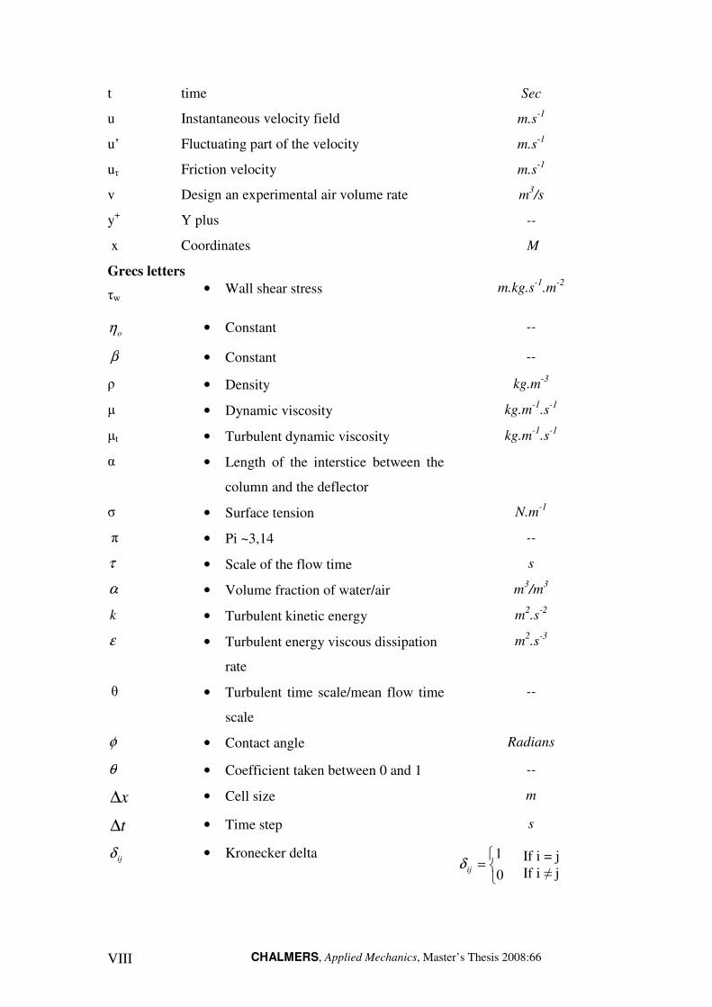
t time Sec

u Instantaneous velocity field m.s-1

u’ Fluctuating part of the velocity m.s-1

uτ Friction velocity m.s-1

v Design an experimental air volume rate m3/s

y+ Y plus --

x Coordinates M

Grecs letters

τw • Wall shear stress m.kg.s

-1.m

-2

oη • Constant --

β • Constant --

ρ • Density kg.m-3

µ • Dynamic viscosity kg.m-1

.s-1

µt • Turbulent dynamic viscosity kg.m-1

.s-1

α • Length of the interstice between the

column and the deflector

σ • Surface tension N.m-1

π • Pi ~3,14 --

τ • Scale of the flow time s

α • Volume fraction of water/air m3/m

3

k • Turbulent kinetic energy m2.s

-2

ε • Turbulent energy viscous dissipation

rate

m2.s

-3

θ • Turbulent time scale/mean flow time

scale

--

φ • Contact angle Radians

θ • Coefficient taken between 0 and 1 --

x∆ • Cell size m

t∆ • Time step s

ijδ • Kronecker delta

=0

1ijδ

If i = j If i ≠ j

CHALMERS, Applied Mechanics, Master’s Thesis 2008:66 IX

USEFUL VOCABULARY

CERT European research center of technology of TOTAL

CFD Computational Fluid Dynamics

Euler/Euler Two-phases model

RNG Renormalization Group method used in a k ε model of turbulence

VOF Volume of fluid (two-phases model)

CHALMERS, Applied Mechanics, Master’s Thesis 2008:66 1

1 Introduction

1.1 Background

The object of the study presented is a good understanding of how to simulate an air and water flow passing through a distributor. The water flow has the particularity to be of different shapes through and downstream the distributor: jets, layers and droplets. This particularity makes, in theory, the usual two-phase CFD models not adapted for the simulation of the whole domain of interest.

1.2 Problem definition and purpose

This study is based on experimental data of air and water flows passing through a distributor. Experiments have been carried out in a previous work. The object of this report is to be able to reproduce with CFD simulations those experiments. The experimental results allow the validation of the CFD simulations.

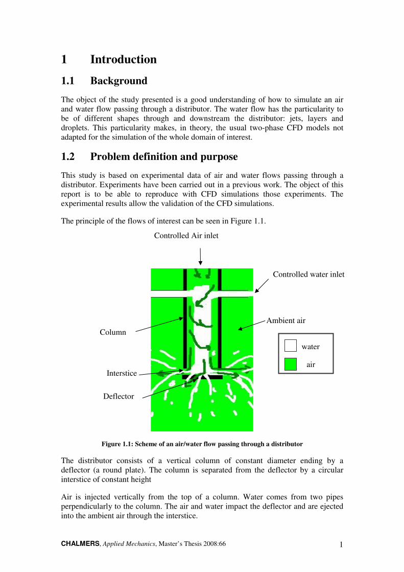
The principle of the flows of interest can be seen in Figure 1.1.

Figure 1.1: Scheme of an air/water flow passing through a distributor

The distributor consists of a vertical column of constant diameter ending by a deflector (a round plate). The column is separated from the deflector by a circular interstice of constant height

Air is injected vertically from the top of a column. Water comes from two pipes perpendicularly to the column. The air and water impact the deflector and are ejected into the ambient air through the interstice.

Column

Controlled water inlet

Ambient air

Controlled Air inlet

water

air

Deflector

Interstice


Depending on the water and air inlet velocities, different phenomena like swirling or spreading of water above the water inlets could appear. The flows are always turbulent at the inlets and unsteady.

1.3 Structure of the report

In Chapter 2 the flows of interest will be presented and discussed. The characteristics of those flows relevant to perform CFD simulation will be pointed out.

In Chapter 3, the models used for the CFD simulations will be presented.

In Chapter 4, we will focus on preliminary CFD studies that have been realized before the entire simulations. Those preliminary studies represent an essential part of this work and have allowed the establishment of the whole settings for the final simulations.

In Chapter the results of nine simulations of the entire geometry will be compared to experimental data. It will then be possible to draw conclusions about this work.


2 Presentation of the flows

2.1 The distributor

In Figure 2.1, the geometry of the experimental distributor can be seen. The distributor is mainly constituted by a column followed by a deflector, as explained in Section 1.2. Air comes from the top of the column after passing an elbow. Water comes in the column by two entrances from flexible pipes.

Figure 2.1: Detailed scheme of the distributor (left view), with air and water path line (right view)

The height of the gap is called α. The other lengths are expressed in function of α. In the Figure 2.1, ones can see that there are large scale differences. For example the distance between the water entrance and the deflector is about thirty times the distance between the column and the deflector.

2.2 The whole domain

We are also interested in the domain downstream the distributor. The way the water is distributed downstream is quantified thanks to a collector. In Figure 2.2 the whole domain is shown. The distributor is placed on the top. After passing the distributor, the flow arrives into ambient air. At a distance of about thirty times the distance between the column and the deflector (i.e. 30*α) a collector is placed. The collector, shown in Figure 2.3, allows the quantification of the quantity of water falling on different area downstream the deflector.

Column

Deflector

Interstice/Gap, height=α

Elbow

Flexible pipe

Water inlet: Ø ~3.α

Water inlet

Air inlet

Ø ~4 α

Distance between water entrances and

the deflector ~ 30.α

Column Ø ~ 10.α


Figure 2.2: Scheme of the distributor in the whole domain of interest

The collector is constituted by 14 recipients. The recipients have concentric ring shapes. The depth of the recipients is about twenty times the distance column/deflector α. In Figure 2.3, one can see the collector from the top.

Figure 2.3: Top view of the collector

The recipients are named by a number. The recipient N°1 is the recipient at the center of the collector and recipient N°14 is the recipient at the edge.

The volumes of water collected in each recipient during a fixed delay constitute the data base that allows comparison with the CFD simulations that is presented in Chapter 5.

Ambient atmosphere:

Distributor

Collector Width of the collector:~250.α

Recipient’s height: ~20. α

Recipient N°1

Recipient N°14


2.3 Material properties

The liquid considered is water at 20° C and atmospheric pressure:

ρwater = 998 kg/m3 and µwater = 0,001 kg/(m s)

The gas is air at 20° C and atmospheric pressure:

ρair = 1,225 kg/m3 and µair = 1.78*10-5 kg/(m s)

The surface tension between water and air is: σ = 0.072 N/m

2.4 Inlet volume flow rates

Different flow rates of air and water have been studied experimentally during a previous study.

4 volumes flow rates of water have been tested; they will be referred to as follow:

V1 < V2 < V3 < V4

9 air volume flow rates have been tested, with a similar notation:

v1<v2 < v3 < v4< v5 < v6 < v7 < v8 < v9

Those volume flow rates constitute the different possibilities of inlets conditions for the CFD simulations.

Remark:

In this report the cases will be named by their water volume rate followed by their air volume rate. For example the case with the water inlet volume rate of “V1” and the air volume rate of “v3” will be called case “V1 v3”.


2.5 Inlet Reynolds Numbers

For an internal flow, the flow is considered to be turbulent for Re > 2300, [3]. The operating conditions are atmospheric pressure and 20 °C. The Reynolds numbers are calculated for one fluid with the diameter of the pipe as a characteristic length, see equation (2.1) and Table 2.1.

µ

ρ diameterpipeUinlet

_**Re_ = (2.1)

Table 2.1: Reynolds numbers at the inlets

Air volume flow rate [m3/s]

Inlet Reynolds number

Water volume flow rate [m3/s]

Inlet Reynolds Number

v1 5200 V1 8782 v2 8700 V2 14072 v3 17400 V3 21158 v4 26100 V4 28243 v5 34800 v6 43500 v7 52200 v8 69600 v9 87000

The Table 2.1 shows that the inlet flows of both air and water are turbulent. A turbulence model will be used for the simulations, see part 3 for more details. The range of Reynolds numbers varies from 5000 to 90 000. From an experiment to another the level of turbulence will not be the same, this could have an impact on the simulations accuracy, for example on the y+ calculation.

2.6 Weber number calculation at the ejection

The Weber number, see equation (2.2), characterizes the relative importance of the aerodynamical forces compared to the surface tension forces. The surface tension σ is a cohesive force which tends to reduce the surface creation of a given liquid volume.

σ

ρ DUWe

g ** 2

= (2.2)

If We >>1 the surface tension effects could be neglected.

At the column outlet (i.e. at the ejection) we can estimate a characteristic length D as the length of the gap between the column and the deflector: i.e. α. The mean velocity is computed by dividing the sum of the water and air volume rates by the passing section area.


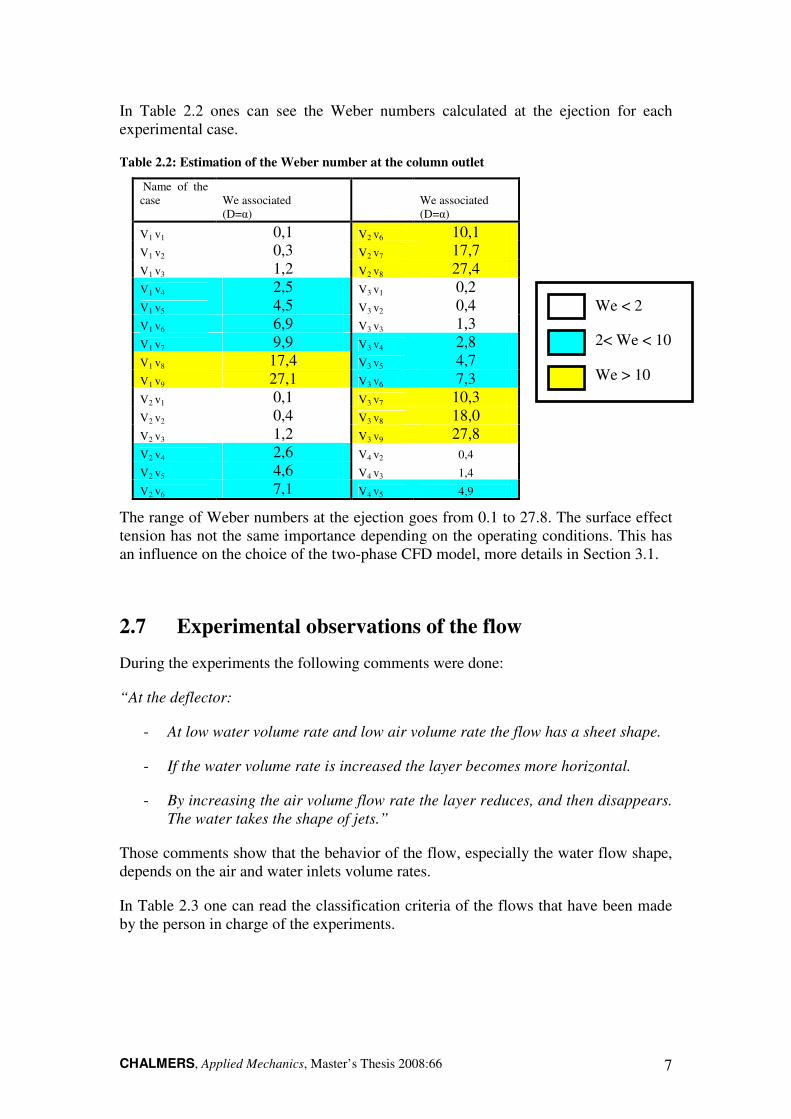
In Table 2.2 ones can see the Weber numbers calculated at the ejection for each experimental case.

Table 2.2: Estimation of the Weber number at the column outlet

Name of the case

We associated (D=α)

We associated (D=α)

V1 v1 0,1 V2

v6 10,1 V1

v2 0,3 V2 v7 17,7

V1 v3 1,2 V2

v8 27,4 V1

v4 2,5 V3 v1 0,2

V1 v5 4,5 V3

v2 0,4 V1

v6 6,9 V3 v3 1,3

V1 v7 9,9 V3

v4 2,8 V1

v8 17,4 V3 v5 4,7

V1 v9 27,1 V3

v6 7,3 V2

v1 0,1 V3 v7 10,3

V2 v2 0,4 V3

v8 18,0 V2

v3 1,2 V3 v9 27,8

V2 v4 2,6 V4

v2 0,4

V2 v5 4,6 V4

v3 1,4

V2 v6 7,1 V4

v5 4,9

The range of Weber numbers at the ejection goes from 0.1 to 27.8. The surface effect tension has not the same importance depending on the operating conditions. This has an influence on the choice of the two-phase CFD model, more details in Section 3.1.

2.7 Experimental observations of the flow

During the experiments the following comments were done:

“At the deflector:

- At low water volume rate and low air volume rate the flow has a sheet shape.

- If the water volume rate is increased the layer becomes more horizontal.

- By increasing the air volume flow rate the layer reduces, and then disappears.

The water takes the shape of jets.”

Those comments show that the behavior of the flow, especially the water flow shape, depends on the air and water inlets volume rates.

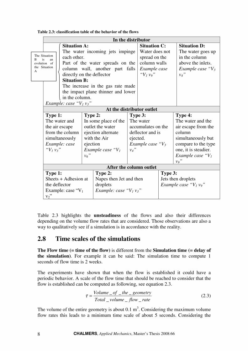
In Table 2.3 one can read the classification criteria of the flows that have been made by the person in charge of the experiments.

We < 2

2< We < 10

We > 10


Table 2.3: classification table of the behavior of the flows

In the distributor

Situation A:

The water incoming jets impinge each other. Part of the water spreads on the column wall, another part falls directly on the deflector Situation B:

The increase in the gas rate made the impact plane thinner and lower in the column.

Example: case “V1 v3”

Situation C:

Water does not spread on the column walls Example case

“V1 v9”

Situation D:

The water goes up in the column above the inlets. Example case “V3

v4”

At the distributor outlet

Type 1:

The water and the air escape from the column simultaneously Example: case

“V1 v3”

Type 2:

In some place of the outlet the water ejection alternate with the Air ejection Example case “V1

v6”

Type 3:

The water accumulates on the deflector and is ejected. Example case “V3

v4”

Type 4:

The water and the air escape from the column simultaneously but compare to the type one, it is steadier. Example case “V1

v9”

After the column outlet

Type 1:

Sheets + Adhesion at the deflector Example: case “V1 v2”

Type 2:

Napes then Jet and then droplets Example: case “V1 v3”

Type 3:

Jets then droplets Example case “V1 v9”

Table 2.3 highlights the unsteadiness of the flows and also their differences depending on the volume flow rates that are considered. Those observations are also a way to qualitatively see if a simulation is in accordance with the reality.

2.8 Time scales of the simulations

The Flow time (= time of the flow) is different from the Simulation time (= delay of

the simulation). For example it can be said: The simulation time to compute 1 seconds of flow time is 2 weeks.

The experiments have shown that when the flow is established it could have a periodic behavior. A scale of the flow time that should be reached to consider that the flow is established can be computed as following, see equation 2.3.

rateflowvolumeTotal

geometrytheofVolume

___

___=τ (2.3)

The volume of the entire geometry is about 0.1 m3. Considering the maximum volume flow rates this leads to a minimum time scale of about 5 seconds. Considering the

The Situation B is an evolution of the Situation A


minimum volume flow rate this leads to a maximum time scale of about 100 seconds. Hopefully it has been observed by CFD that the real flow time of establishment of the flow is much lower. To get a good estimation we should only consider the column volume which is about 0.001 m3. This leads to a theoretical minimum time scale of simulation of 0.2 seconds and a maximum of about 4 seconds.

In absence of other indicators1, it is good to simulate at least 2 time scales of flow. To be sure that the flow is fully developed, monitoring of the volume fraction of water at the column outlet have been made.

To perform an unsteady simulation the software needs a time step, t∆ . It could be established by the software as it is presented in the Part 3.3 or it can be fixed by the user. A good estimation of the suitable time step is given by the following relation (2.4):

maxV

xt

∆=∆

(2.4)

Where x∆ is the length of the cell in the flow direction and Vmax is the maximal velocity. For the simulations Vmax can be estimated as the mean velocity in the interstice between the column and the deflector. The minimum cell length in the gap is about α/10. The time step will be around 10-4 seconds for most of the simulations of the entire geometry.

1 As a mass flow balance.


3 CFD settings to resolve an unsteady, two-phase,

turbulent flow

3.1 The multiphase models

There are three main models to resolve a multiphase flow: The Volume Of Fluid approach (VOF), the Euler/Euler (E/E) approach and the Euler/Lagrange approach. In this report we will focus on the VOF and the E/E approaches because they are the models retained during previous investigations.

3.1.1 Basic notions in two-phase flows

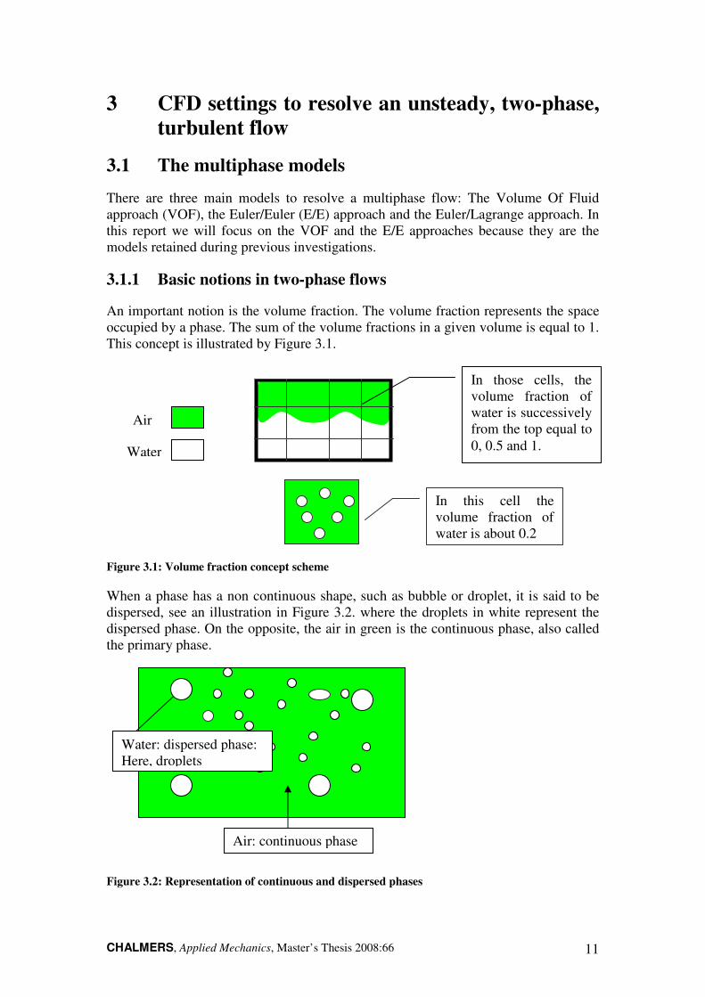
An important notion is the volume fraction. The volume fraction represents the space occupied by a phase. The sum of the volume fractions in a given volume is equal to 1. This concept is illustrated by Figure 3.1.

Figure 3.1: Volume fraction concept scheme

When a phase has a non continuous shape, such as bubble or droplet, it is said to be dispersed, see an illustration in Figure 3.2. where the droplets in white represent the dispersed phase. On the opposite, the air in green is the continuous phase, also called the primary phase.

Figure 3.2: Representation of continuous and dispersed phases

Air: continuous phase

Air

Water

In those cells, the volume fraction of water is successively from the top equal to 0, 0.5 and 1.

In this cell the volume fraction of water is about 0.2

Water: dispersed phase: Here, droplets


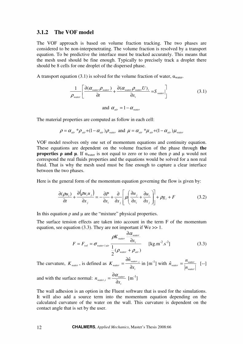
3.1.2 The VOF model

The VOF approach is based on volume fraction tracking. The two phases are considered to be non-interpenetrating. The volume fraction is resolved by a transport equation. To be predictive the interface must be tracked accurately. This means that the mesh used should be fine enough. Typically to precisely track a droplet there should be 8 cells for one droplet of the dispersed phase.

A transport equation (3.1) is solved for the volume fraction of water, αwater.

=

∂

∂+

∂

∂water

i

iwaterwaterwaterwater

water

Sx

U

t

)()(1 ραρα

ρ (3.1)

and waterair αα −= 1

The material properties are computed as follow in each cell:

waterairairair ραραρ )1(* −+= and waterairairair µαµαµ )1(* −+=

VOF model resolves only one set of momentum equations and continuity equation. These equations are dependent on the volume fraction of the phase through the

properties ρ and µ. If αwater is not equal to zero or to one then ρ and µ would not correspond the real fluids properties and the equations would be solved for a non real fluid. That is why the mesh used must be fine enough to capture a clear interface between the two phases.

Here is the general form of the momentum equation governing the flow is given by:

( )Fg

x

u

x

u

xx

P

x

uu

t

ui

j

i

i

j

jij

jii ++

∂

∂+

∂

∂

∂

∂+

∂

∂−=

∂

∂+

∂

∂ρµ

ρρ )( (3.2)

In this equation ρ and µ are the “mixture” physical properties.

The surface tension effects are taken into account in the term F of the momentum equation, see equation (3.3). They are not important if We >> 1.

)(2

1/

airwater

i

water

water

airwatervol

xK

FF

ρρ

αρ

σ

+

∂

∂

== [kg.m-2.s-2] (3.3)

The curvature, waterK , is defined as i

iwater

waterx

nK

∂

∂=

,ˆin [m-1] with

water

water

watern

nn =ˆ [--]

and with the surface normal: i

water

iwaterx

n∂

∂=

α, [m-1]

The wall adhesion is an option in the Fluent software that is used for the simulations. It will also add a source term into the momentum equation depending on the calculated curvature of the water on the wall. This curvature is dependent on the contact angle that is set by the user.


Figure 3.3: Contact angle

The contact angle is the angle Φ made by a drop of liquid in presence of a gas and a solid, see Figure 3.3. This angle depends on the liquid, gas and solid surface, properties. If Φ< 90° the surface is hydrophilic, water spreads easily. On the contrary if Φ > 90° the surface is hydrophobic. At the column outlet the contact angle creates a curvature that can have importance on the droplets formation.

3.1.3 The Euler/Euler model

The Eulerian model is used for the modeling of separate miscible phases. The two phases could be present in the same cell of calculation without being an interface. An Eulerian treatment is used for each phase.

A mass conservation, equation (3.4), is solved for the water phase, with the constraint that the sum of the volume fractions is equal to one.

0)()(1

=

∂

∂+

∂

∂

i

iwaterwaterwaterwater

water x

u

t

ραρα

ρ (3.4)

1=+ airwater αα

Contrary to the VOF model, the following momentum equation is valid for the velocity field of air (with α=αair and ρ=ρair) and for the velocity field of water (with α=αwater and ρ=ρwater). This leads to three equations for the air phase and three equations for the water phase. Six equations are solved for the mean flow, see equation (3.5).

( )iiiij

j

j

i

j

j

i

jij

jii FRgx

u

x

u

x

u

xx

P

x

uu

t

u+++

∂

∂−

∂

∂+

∂

∂

∂

∂+

∂

∂−=

∂

∂+

∂

∂αρδµαµα

αραρ

3

2)( (3.5)

“R” is the interaction force between the two phases. “P” is the pressure shared by the two phases. “F” refers to other forces like external body forces; lift force, virtual mass force. They are optional in fluent and negligible in our case.

If the equations are solved for water then )(* ,,/ wateriairiwaterairi uuKR −= .

The term Kair/water is computed following the equation (3.6). airwaterwaterair KK // = so if

the equations are solved for air then )(* ,,/ airiwateriwaterairi uuKR −= .

p

waterwaterair

waterair

fK

τ

ραα=/ [kg/m3s] (3.6)

Gas (air)

Liquid (water)

Solid (wall)

Φ


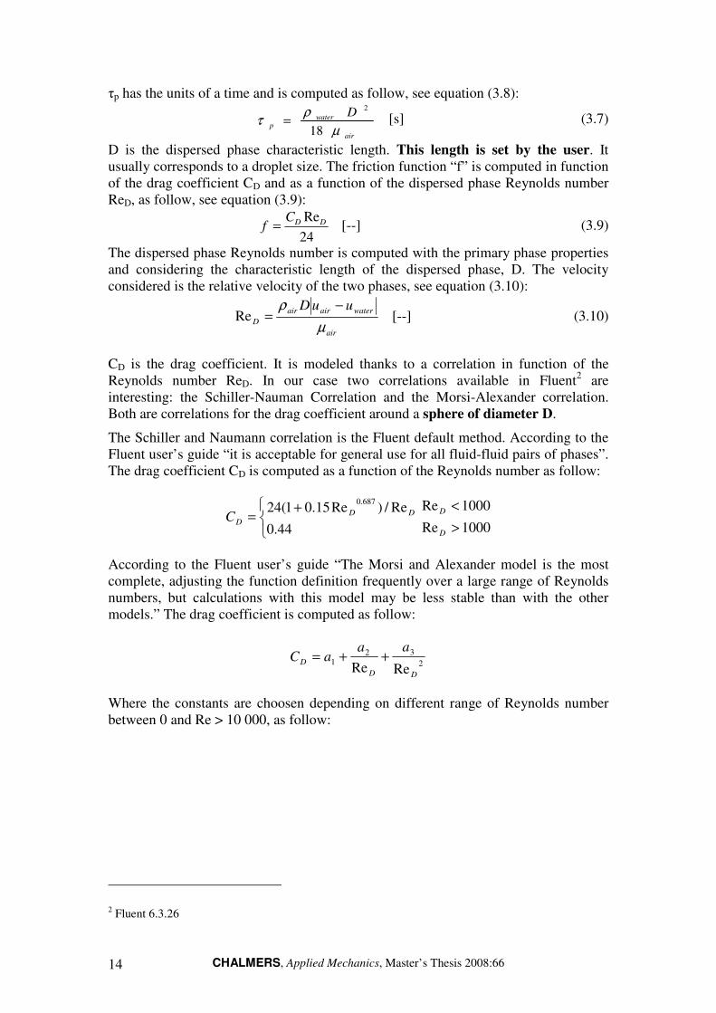
τp has the units of a time and is computed as follow, see equation (3.8):

air

waterp

D

µ

ρτ

18

2

= [s] (3.7)

D is the dispersed phase characteristic length. This length is set by the user. It usually corresponds to a droplet size. The friction function “f” is computed in function of the drag coefficient CD and as a function of the dispersed phase Reynolds number ReD, as follow, see equation (3.9):

24

ReDDCf = [--] (3.9)

The dispersed phase Reynolds number is computed with the primary phase properties and considering the characteristic length of the dispersed phase, D. The velocity considered is the relative velocity of the two phases, see equation (3.10):

air

waterairair

D

uuD

µ

ρ −=Re [--] (3.10)

CD is the drag coefficient. It is modeled thanks to a correlation in function of the Reynolds number ReD. In our case two correlations available in Fluent2 are interesting: the Schiller-Nauman Correlation and the Morsi-Alexander correlation. Both are correlations for the drag coefficient around a sphere of diameter D.

The Schiller and Naumann correlation is the Fluent default method. According to the Fluent user’s guide “it is acceptable for general use for all fluid-fluid pairs of phases”. The drag coefficient CD is computed as a function of the Reynolds number as follow:

+

=44.0

Re/)Re15.01(24687.0

DDDC

1000Re

1000Re

>

<

D

D

According to the Fluent user’s guide “The Morsi and Alexander model is the most complete, adjusting the function definition frequently over a large range of Reynolds numbers, but calculations with this model may be less stable than with the other models.” The drag coefficient is computed as follow:

2

321

ReReDD

D

aaaC ++=

Where the constants are choosen depending on different range of Reynolds number between 0 and Re > 10 000, as follow:

2 Fluent 6.3.26


3

Ri is increased if D is decreased. The physic sense of this is that has less drag effect on a big droplet whereas small droplets are easily dragged by the air flow.

The setting of “D” by the user is important. For a two-phase flow where the liquid phase is really formed by droplets “D” could be taken to be a droplet size. In our case the flow has not the same shape into the distributor and downstream the distributor. The shape of the liquid phase depends also on the considered case, as it is explained in the Chapter Two. This form of the Euler/Euler model does not take into account the surface tension effects.

3 Fluent user’s guide.


3.2 The RNG k-ε turbulence model

3.2.1 The Reynolds Averaged Navier Stokes (RANS) approach

When the flow is turbulent the number of unknowns into the Reynolds Averaged Naviers-Stokes equations exceeds the number of equations. For this reason two equations are added which are models for the turbulent kinetic energy calculation (k) and the turbulent viscous dissipation calculation (ε).

The principle of the RANS approach is to consider the instantaneous velocity field ui as the sum of a mean U (time averaged) and a fluctuating part u’: ui= Ui +ui’as it is illustrated in Figure 3.2.

The total velocity

-4,0E-01

-2,0E-01

0,0E+00

2,0E-01

4,0E-01

6,0E-01

8,0E-01

1,0E+00

1,2E+00

1,4E+00

0

0,0

5

0,1

0,1

5

0,2

0,2

5

0,3

0,3

5

0,4

0,4

5

time [-]

Ve

loc

ity

[-] the instantenous

velocity U'

the fluctating part u'

The mean velocity U

Figure 3.4: Overlay of the Reynolds decomposition of the velocity

By replacing the instantaneous velocity ui by the sum of the mean and the fluctuating part of the instantaneous velocity into the Navier-Stokes equations and time

averaging, the terms ''jiuu appear. These terms are called Reynolds stresses. They

must be modeled to close the RANS equations.

By means of mathematical operations well described in the literature, two equations are established: one for the turbulent kinetic energy k and one for the turbulent kinetic energy dissipation rate ε. Modeling assumptions are made to resolve the set of equations.

u’

u

U

� u=U+u’


3.2.2 The Boussinesq Approach

The kinetic energy k associated with the turbulence is defined as :

++=

2'3

2'2

2'1

2

1uuuk [m2/s2] (3.11)

The turbulent viscous dissipation rate of kinetic energy ε is defined as:

ijij ss**2ρ

µε = [m2/s3] (3.12)

with

∂

∂+

∂

∂=

i

j

j

i

ijx

U

x

US

2

1 and

∂

∂+

∂

∂=

i

j

j

i

ijx

u

x

us

''

2

1 [s-1]

Turbulence enhances transport of momentum similar to the molecular transport of momentum by viscosity. By analogy the Reynolds stresses could be related to the mean flow by the effect of a modeled “turbulent viscosity” µt, see equation (3.13):

ijij

k

k

ijtji kx

USuu δρδµρ

3

2)

3

22(* −

∂

∂−=− (3.13)

The idea is that µt [kg/(m.s)], the turbulent dynamic viscosity, can be expressed as a product of a turbulent velocity scale u’ [m/s] and a length scale l [m], i.e.:

lut '**ρµ ∝

If one velocity scale and one length scale suffice to describe the effects of turbulence dimensional analysis yields:

ερµ µ

2k

Ct = with ku =' and ε

2/3k

l =

3.2.3 RNG k-ε model

The k-ε model proposes to resolve a transport equation for k and a transport equation for ε. The RNG k ε model proposes improvements for the calculation of the ε transport equation.

The following equation is solved for k; the turbulent kinetic energy:

( )ρεµα

ρρ−+

∂

∂

∂

∂=

∂

∂+

∂

∂k

j

effk

jj

jP

x

k

xx

kU

t

k )( (3.14)

With 22 ijtk SP µ= [kg.m/s3], the turbulent kinetic energy production rate by the mean

flow.

kα and εα are the inverse effective Prandtl numbers for k and ε, respectively.

They are calculated using a formula derived analytically by the RNG theory (if they


are taken constant kα = εα =1.39). The scale elimination procedure in RNG theory

results in an “analytically-derived differential formula for effective viscosity that accounts for low-Reynolds-number effects” for the calculation of the effective

viscosity: teff µµµ += and leads toε

ρµ µ

2k

Ct = for high Reynolds flow.4

The following equation is solved for ε, the turbulent viscous dissipation rate of kinetic energy, see equation (3.15):

( ) ( ) ( )ρεεε

µαρερε

εεε

*

21 CPCkxxx

U

tk

j

eff

jj

j−+

∂

∂

∂

∂=

∂

∂+

∂

∂ (3.15)

The constants: 42.11 =εC , *

2εC , are derived using the Renormalization Group method.

Compared to a standard k-ε model a RNG k-ε model introduce a new variable η as

flow

turbulentkS

τ

τ

εη == . ijij SSS 2= [s-1] with

∂

∂+

∂

∂=

i

j

j

i

ijx

U

x

US

2

1 [s-1] is the inverse

of the time scale related to the mean flow deformation and ε

k [s] is the turbulent time

scale representing the largest turbulent structures.

If η>1 the mean flow changes are faster than the turbulence, on the contrary if η < 1 the turbulence time scale is the smallest time scale, turbulence changes are faster than mean flow changes.

This ratio is taken into account in the turbulent kinetic dissipation rate by the

variable *

2εC , computed following the equation (3.16):

3

3

2

*

21

1

βη

η

ηρηµ

εε+

−

+=o

C

CC (3.16)

38.4=oη , 012.0=β 68.12 =εC

By this way according to the Fluent user’s guide “the RNG model is more responsive to the effects of rapid strain and streamline curvature than the standard k-ε model, which explains the superior performance of the RNG model for certain classes of flows.”

4 More details, in the Fluent user’s guide.


Before the deflector the flow changes direction very rapidly and Reynolds numbers can be low because of the small size of the gap:

The model k ε RNG is used by default. The computations are made for industrial applications and need rapid calculations. The RNG method seems to be the best for our calculation.

Remark: VOF and Euler/Euler specificities

For a VOF simulation the k-ε equations are resolved for the mixture.

For an Euler/Euler simulation the k ε equations can be solved for each phase at

each cell with the option per phase or only for the primary phase, by taken into account the influence of the dispersed phase on the primary phase, with the option dispersed. The option per phase has been tested and it is too much time consuming. The turbulence resolution is a limitation of the Euler/Euler simulation presented here.

3.2.4 The wall effect treatment

y+ is a dimensionless number that allows using similarity properties for boundary layers. Indeed a wall has an effect on the velocity and turbulence that must be modeled.

It is therefore important to use the good relation at the good place. The nodes of the mesh placed near the wall boundary conditions should therefore satisfy y+ criteria corresponding to the near-wall modeling approaches. They should have goods y to get good y+ values.

To resolve the boundary layer, wall treatments are proposed by fluent. In our cases, unsteady, two-phases and time consuming it is very difficult to design a proper grid in accordance with the wall treatment model, i.e. with the good y+. However the boundary layer has never enough time to become developed in particularly in the gap between the deflector and the column.

Because most of the experimental cases have a low air-Reynolds number in the interstice a low Reynolds number wall treatment is used.

The setting of the y+ is a limitation of the following simulations and seems to be the cause of convergence problems. It has been remarked that the residuals of the turbulence properties were higher than the others.

Deflector

Flow higher component direction

Column

Area of rapid strain and streamline curvature


3.3 The transient solver

3.3.1 Presentation of the resolution schemes5

General equation for transport of a scalar (for example α, k, ε, U, V, W:

( ) φφφρρφ Sxx

Uxt ii

i

i

+∂

∂Γ

∂

∂=

∂

∂+

∂

∂)()( (3.17)

In order to be solved this equation (3.17) is integrated in time and in space. What is important to notice is that an assumption is made. The time step is small enough to consider that the scalar is constant over the time step, see equation (3.18)

tdt PP

tt

t

p ∆−+=∫∆+

])1([ 01 φθθφφ (3.18)

If θ =0 the scheme is said to be explicit. If 10 ≤< θ the scheme is said to be implicit, with a particularity if θ =0.5 the scheme is called Crank-Nicolson. If θ =1 the scheme is said to be fully implicit.

Implicit methods tolerate much larger time step for comparable accuracy. The Crank Nicholson Method should be preferred because it is more accurate (2nd order accurate due to θ =0.5) however it requires more intermediate iterative stages.

In all the simulations presented here the implicit method has been used.

3.3.2 Variable time step for VOF simulations

The Courant Number, CN, see equation (3.19), is a dimensionless number that compares the time step in a calculation to the time needed by a fluid element to travel across a control volume:

fluidcell Vx

tCN

/∆

∆= (3.19)

Typically for a good simulation CN should be equal to 2. Fluent is able to increase or decrease the time step to respect this criteria.

This method is used for the quarter of volume VOF simulations presented in Chapter 4.

5 Ref [1] chapter 8

• Index 0 means old time value. • Index1 means new time value. • Index p means that the value is taken at

the point (cells) P.

• θ is taken between 0 and 1


3.3.3 Adaptive time stepping for Euler/Euler simulations

For an Euler/Euler simulation, instead of the CN the software estimates the truncation error:

• After one time step the truncation error associated with the time step is calculated. It is an estimation of the difference between the calculated variable in one cell and the variable that should have been computed with a perfect accordance to the new values of the neighborhood cells variables.

If the truncation error value is under a fixed value (0.01 by default) the time step is increased. On the contrary if the truncation error is above the limit value, the time step is decreased.

This method has been used for the simplified Euler/Euler simulations presented in the Chapter 4.

Unfortunately it is too time consuming to use it efficiently for the entire Euler/Euler simulation presented in Chapter 5. It has been used when there where convergence problems.


4 Preliminary studies

Before trying to realize entire simulations it is important for the user to be acquainted with the problem and the software possibilities. In this chapter are presented CFD studies that have been performed before simulations of the entire geometry. The principle is to solve simpler flows to focus on one aspect of the problem. This is also the occasion for a novice to get acquainted with the software without having to deal with a heavy geometry. Those studies are the ground of the entire simulations presented in Chapter 5.

4.1 Estimation of the optimized grid: mono-phase 2D

simulations

4.1.1 Purposes of the study

In simulations performed before this study, the number of cells in height of the interstice between the deflector and the column was 4. This number seems too low to describe correctly the flow but has the advantage of reducing the calculation time. In 3D it is not possible to have a very fine mesh. A fine mesh reduces the theoretical time step, see section 2.4; and increases the number of cells. This adds calculation time.

A 2D axi-symmetric study on an air flow has been performed to get an idea of a reasonable number of cells in the interstice.

4.1.2 Approach

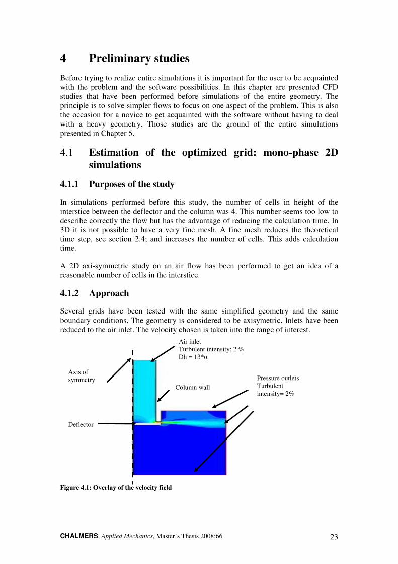
Several grids have been tested with the same simplified geometry and the same boundary conditions. The geometry is considered to be axisymetric. Inlets have been reduced to the air inlet. The velocity chosen is taken into the range of interest.

Figure 4.1: Overlay of the velocity field

Axis of symmetry

Deflector

Air inlet Turbulent intensity: 2 % Dh = 13*α

Pressure outlets Turbulent intensity= 2%

Column wall


In Figure 4.1, the contour of the velocity field obtained is shown and the boundary conditions are presented. By looking at this picture it can be seen that the pressure outlet above the deflector is too close from the interstice. For the entire simulation this will be taken into account and the top pressure outlet will be placed further away.

In Figure 4.2, two tested grid are presented. On the left hand side there is a grid with ten cells in the interstice. On the right hand side there is a grid with forty cell in the interstice. This second grid is considered to give the best results and is therefore the reference of this study.

Figure 4.2: Example of tested grids

4.1.3 Main results

In Figure 4.3 the radial velocity predicted by 4 different grids, at the interstice (the gap), is presented. The important characteristics of those grids are given in the legendary at right. A coarse grid with four cells at the interstice, the reference grid with forty cells at the interstice, a grid with eleven cells refined near the wall and a grid with ten cells of the same height are compared. The grid with eleven cells allows comparing the importance of the near wall refinement.

Figure 4.3: Comparison of the radial velocity at the column outlet

Optimized grid 10 cells of α/10 in the gap

A fine grid: 40 cells of α/100 mm in the gap

α4

1 α

4

2 α4

3 α


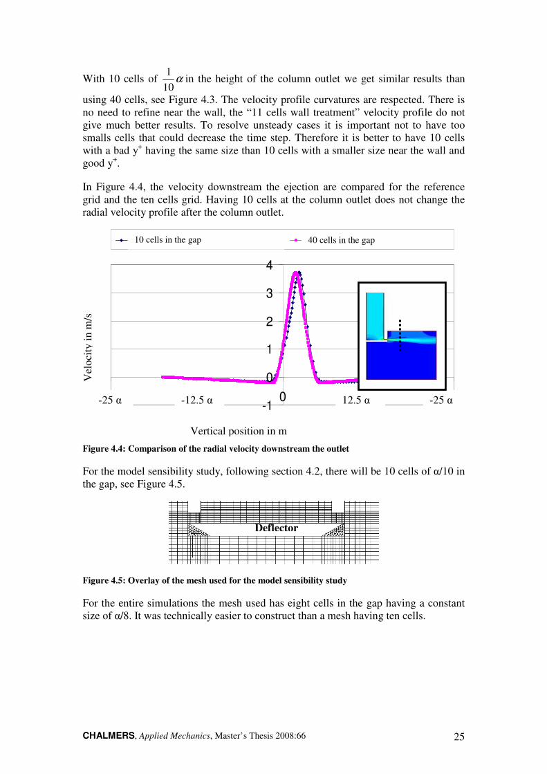
With 10 cells of α10

1in the height of the column outlet we get similar results than

using 40 cells, see Figure 4.3. The velocity profile curvatures are respected. There is no need to refine near the wall, the “11 cells wall treatment” velocity profile do not give much better results. To resolve unsteady cases it is important not to have too smalls cells that could decrease the time step. Therefore it is better to have 10 cells with a bad y+ having the same size than 10 cells with a smaller size near the wall and good y+.

In Figure 4.4, the velocity downstream the ejection are compared for the reference grid and the ten cells grid. Having 10 cells at the column outlet does not change the radial velocity profile after the column outlet.

Figure 4.4: Comparison of the radial velocity downstream the outlet

For the model sensibility study, following section 4.2, there will be 10 cells of α/10 in the gap, see Figure 4.5.

Figure 4.5: Overlay of the mesh used for the model sensibility study

For the entire simulations the mesh used has eight cells in the gap having a constant size of α/8. It was technically easier to construct than a mesh having ten cells.

Deflector

-1

0

1

2

3

4

-0,1 -0,05 0 0,05 0,1

position verticale

vit

es

se

en

m/s

10 cellules dans l'interstices 40 cellules dans l'interstice10 cells in the gap 40 cells in the gap

Vel

ocit

y in

m/s

-25 α -12.5 α 12.5 α -25 α

Vertical position in m


4.2 Comparison of VOF simulations and Euler/Euler

simulations

The mesh used for the following simulations is presented in Appendix N°2.

4.2.1 Purposes of the study

The objective of this study is to compare VOF simulations and Euler/Euler simulations for two different inlet conditions. The geometry is considered to have two symmetry planes. We focus on the interior of the distributor and the column outlet, see Figure 4.6.

The tested cases are the case “V1 v3” and the case “V1 v9”. Those cases have the same water volume rate V1 and different air volume rate. For the case “V1 v9” the surface tension is expected to be negligible We >> 1 whereas for the case “V1 v3” it should be predominating We < 1 as presented in the Table 2.2.

The settings that are compared are presented in Table 4.1.

Table 4.1: Compared case settings

V1 v9

Case name Model Diameter of the dispersed

phase D

CD correlation Contact angle

D= α*2.5 E/E Α*2.5 S. N. -- D= α/2 E/E α/2 S. N. --

D= α*2.5 M.A. E/E Α*2.5 M. A. -- VOF 90 V.o.F -- -- 90°

VOF 120 V.o.F -- -- 120°

V1 v3

Case name Model Diameter of the dispersed

phase D

CD correlation Contact angle

D= α*2.5 E/E α*2.5 S. N. -- D= α/2 E/E α/2 S. N. -- VOF 90 V.o.F -- -- 90°

VOF 120 V.o.F -- -- 120°

For the Euler/Euler simulations, two diameters of the dispersed phase and the correlation for the drag coefficient are tested. The influence of the correlation on the time of calculation is observed. The comparison with the VOF simulations should help us to choose the best characteristic length of the dispersed phase, i.e. “D”, to set into future Euler/Euler simulations.

For the VOF simulations two different contact angles (90° and 120°) between the water and the wall are tested. It highlights the importance of the surface tension effect at the wall.


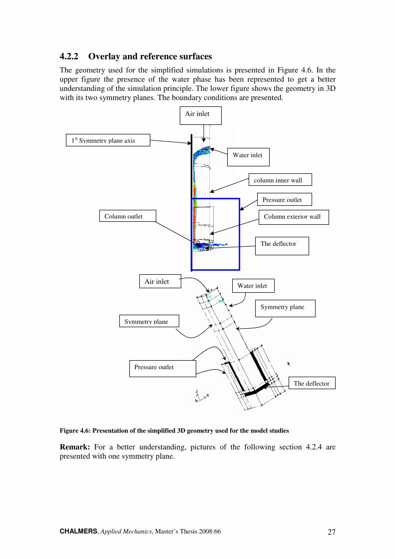
4.2.2 Overlay and reference surfaces

The geometry used for the simplified simulations is presented in Figure 4.6. In the upper figure the presence of the water phase has been represented to get a better understanding of the simulation principle. The lower figure shows the geometry in 3D with its two symmetry planes. The boundary conditions are presented.

Figure 4.6: Presentation of the simplified 3D geometry used for the model studies

Remark: For a better understanding, pictures of the following section 4.2.4 are presented with one symmetry plane.

The deflector

Column outlet

Pressure outlet

1st Symmetry plane axis

Water inlet

Air inlet

column inner wall

Column exterior wall

Symmetry plane

Symmetry plane

The deflector

Pressure outlet

Water inlet Air inlet


4.2.3 Estimation of the establishment flow time

During the simulation the column outlet has been monitored as a function of the flow time to see if a fully developed state is reached. On the following Figure 4.7 and Figure 4.8, ones can see those monitors. When a fully developed state is reached it is possible to proceed to the post treatment of the results.

Figure 4.7: History of the volume area weighted volume fraction of air at the column outlet, case

“V1 v3”

Figure 4.8: History of the area weighted velocity of water at the column outlet, case “V1 v9”

The simulation flow time necessary for the slower case “V1 v3”, see Figure 4.7, is

around 0.5 sec. It is about three times the delay needed for the faster case “V1 v9”, see Figure 4.8.

Remark: Depending on the cases the simulation times are included between ten and twenty days for each simulation. The “Morsi and Alexander” correlation does not

increase the simulation time. The VOF. simulations are faster than the Euler/Euler simulations (fewer equations for the same number of cells).

Fully developed state

Fully developed state


It is difficult to be more descriptive about the simulation cost. The simulations are sometimes stopped for various reasons: sharing of the calculation licenses with the other users, divergence of the calculation, technical problems.

4.2.4 Qualitative results for the high air flow case “V1 v9”

Here overlays of the results for the high air flow rate case are presented. figures of the VOF simulation are followed by figures of the Euler/Euler simulations.

Figure 4.9: Contours of volume fraction of water for two VOF simulations with different contact

angle, case “V1 v9”

In Figure 4.9 the presence of water in the distributor is represented for the two VOF simulations. The shape of the water phase is similar. The influence of the contact angle can be seen at the wall, as indicated on the figure. For a contact angle of 90° the water spreads more easily whereas the contact surface is bigger than for the case VOF 120 °.

Figure 4.10: Volume fraction of Water, Euler simulations with different values of the dispersed

phase characteristic length and correlations for the drag coefficient, case “V1 v9”

In Figure 4.10 the presence of water is represented for the three Euler/Euler simulations. The shape of the water phase is similar.

90°

D =α*2.5 D =α/2 D =α*2.5 M. and A. correlation

120°

Wall of the column

Deflector

Water spreads on the column wall The contact surface is bigger for the VOF 90° case


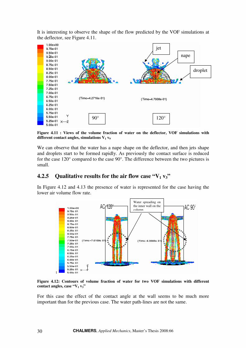
It is interesting to observe the shape of the flow predicted by the VOF simulations at the deflector, see Figure 4.11.

Figure 4.11 : Views of the volume fraction of water on the deflector, VOF simulations with

different contact angles, simulations V1 v9

We can observe that the water has a nape shape on the deflector, and then jets shape and droplets start to be formed rapidly. As previously the contact surface is reduced for the case 120° compared to the case 90°. The difference between the two pictures is small.

4.2.5 Qualitative results for the air flow case “V1 v3”

In Figure 4.12 and 4.13 the presence of water is represented for the case having the lower air volume flow rate.

Figure 4.12: Contours of volume fraction of water for two VOF simulations with different

contact angles, case “V1 v3”

For this case the effect of the contact angle at the wall seems to be much more important than for the previous case. The water path-lines are not the same.

90° 120°

jet

nape

droplet

Water spreading on the inner wall on the column


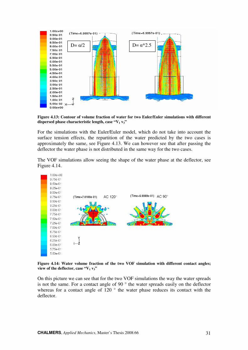
Figure 4.13: Contour of volume fraction of water for two Euler/Euler simulations with different

dispersed phase characteristic length, case “V1 v3”

For the simulations with the Euler/Euler model, which do not take into account the surface tension effects, the repartition of the water predicted by the two cases is approximately the same, see Figure 4.13. We can however see that after passing the deflector the water phase is not distributed in the same way for the two cases.

The VOF simulations allow seeing the shape of the water phase at the deflector, see Figure 4.14.

Figure 4.14: Water volume fraction of the two VOF simulation with different contact angles;

view of the deflector, case “V1 v3”

On this picture we can see that for the two VOF simulations the way the water spreads is not the same. For a contact angle of 90 ° the water spreads easily on the deflector whereas for a contact angle of 120 ° the water phase reduces its contact with the deflector.

D= α/2 D= α*2.5


4.2.6 Post-treatment to compare the VOF and the Euler/Euler cases

The objective is to compare the water radial velocity at the column outlet.

It is difficult to compare a VOF simulation with an Euler/Euler simulation, because the resolved variables are not the same. For an Euler/Euler case the velocity of each phase is computed for each cell whereas for a VOF case only one velocity is computed for each cell, (see Chapter 3).

For the Euler/Euler simulations the water velocity is calculated by taken into account only the cells where 0.1 < αwater ≤ 1, in order to take into account in the calculation only the cells for which the amount of water is significant. As in our case the interface between air and water is distinct for Euler/Euler simulation (Figure 4.15 and Figure 4.16), the influence of the value of 0.1 for αwate is negligible. The area-weighted average of the water radial-velocity is then computed for the cells in the range. The Figure 4.15 shows that at the column outlet only few cells have a water volume fraction superior to 0 and inferior to 0,1 for an Euler/Euler simulation.

Figure 4.15 : Volume fraction of water contours at the column outlet, E/E simulation

For a VOF simulation the cells taken into account for the calculation of the radial surface verify 0,5 < αwater<1. On these cells we can consider that water is predominating into the mixture and therefore the velocity is the water velocity. The area-weighted average of the radial-velocity is then computed. The detailed data are in appendix n°2. The Figure 4.15 shows that at the column outlet almost no cells have a volume fraction superior to zero and inferior to 0,5 for a VOF simulation.

Figure 4.16 : Volume fraction of water at the column outlet, VOF simulation


4.2.7 Quantitative results of the case “V1 v9” simulations

Table 4.1 allows the comparison of the averaged (time and space) radial velocities and velocity magnitudes at the column outlet. To compute the area average water velocity only the cells where there is effectively water are considered, as it is explained in section 4.2.6. For these operating conditions, the simulated flow stabilizes rapidly. The values reported in Table 4.1 have been computed by making a sampling of about ten values taken at regular intervals between the flow time 0.45 and 0.5 sec, because the flow is established but periodic, see Figure 4.7 and Figure 4.8. At these times the simulation has reached a fully developed state.

Table 4.1 : Comparison of the radial velocity and the velocity magnitude at the column outlet for

five different settings and for the inlet conditions V1 v9

Water

Air

Simulation name Radial

Velocity m/s

Velocity magnitude

m/s Radial

Velocity m/s

Velocity magnitude

m/s D=α*2.5 S.N. 1,85 2,23 23,04 24,12 D=α*2.5 S.N. 1,61 2,01 23,77 25,05 D=α/2 MA 1,64 2,03 23,89 25,20 VOF 120 1,96 2,01 22,00 22,74 VOF 90 1,87 1,94 21,80 22,91

The simulation “VOF 90” is taken as the reference to calculate the difference in the velocities predicted by the different models. The “Difference” in percent is calculated with the following relation, see equation (4.1).

( )100*

_

_

refVrad

VradrefVradDifference

−= (4.1)

Table 4.2 Differences of the simulations water radial velocities in percent compared to the VOF

90 simulation, case “V1 v9”

Simulation name Difference

Case D=α*2.5 S.N. -1 %

Case D=α*2.5 S.N. -13 %

Case D=α/2 MA -12 %

VOF 120 +4,8 %

VOF 90 0

Table 4.2 presents the difference in percent of the simulation water radial velocity compared to the VOF 90 simulation. The velocities predicted by the model are similar with at most 13 % of difference. The “Differences” are not especially marked.

The E/E D= α/2 S.N. compare to the VOF 90° gives a closer water radial velocity.

For the Euler/Euler simulations, multiplying D by 5 reduces the velocity of ~12 %.


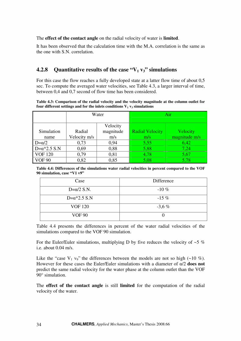
The effect of the contact angle on the radial velocity of water is limited.

It has been observed that the calculation time with the M.A. correlation is the same as the one with S.N. correlation.

4.2.8 Quantitative results of the case “V1 v3” simulations

For this case the flow reaches a fully developed state at a latter flow time of about 0,5 sec. To compute the averaged water velocities, see Table 4.3, a larger interval of time, between 0,4 and 0,7 second of flow time has been considered.

Table 4.3: Comparison of the radial velocity and the velocity magnitude at the column outlet for

four different settings and for the inlets conditions V1 v3 simulations

Water

Air

Simulation name

Radial Velocity m/s

Velocity magnitude

m/s Radial Velocity

m/s Velocity

magnitude m/s D=α/2 0,73 0,94 5,55 6,42 D=α*2.5 S.N 0,69 0,88 5,88 7,24 VOF 120 0,79 0,81 4,78 5,67 VOF 90 0,82 0,85 5,08 5,78

Table 4.4: Differences of the simulations water radial velocities in percent compared to the VOF

90 simulation, case “V1 v9”

Case Difference

D=α/2 S.N. -10 %

D=α*2.5 S.N -15 %

VOF 120 -3,6 %

VOF 90 0

Table 4.4 presents the differences in percent of the water radial velocities of the simulations compared to the VOF 90 simulation.

For the Euler/Euler simulations, multiplying D by five reduces the velocity of ~5 % i.e. about 0.04 m/s.

Like the “case V1 v9” the differences between the models are not so high (~10 %). However for these cases the Euler/Euler simulations with a diameter of α/2 does not predict the same radial velocity for the water phase at the column outlet than the VOF 90° simulation.

The effect of the contact angle is still limited for the computation of the radial velocity of the water.


4.2.9 Conclusions of the quarter of geometry study

This study does not give irrefutable results due to the lack of precision of the results6 compared to the low level of differences (~ 10 %) between the models. However, interesting and clear tendencies can be underlined:

• By looking at the views of the VOF simulations it can be remarked that for the case “V1 v3” the contact angle change the shape of the water spreading on the inner wall of the column. As expected for the angle 120 ° the surface is more hydrophobic and leads to a reduction of the surface of spreading.

• Using a dispersed phase diameter D of α*2.5 instead of α/2 decreases the water ejection velocity for both operating conditions. For the case “V1 v9” this decrease is more important than for the case “V1 v3”. Indeed, the aerodynamical forces are more important for the case “V1 v9”.

• For the case “V1 v9” the model E/E D=α/2 has only 1 % of difference with the

VOF simulation. For the case “V1 v3” the difference reaches 10%. This seems to indicate that for a case where the Weber number at the column outlet is important (~27) the model influence between a VOF and an E/E D= α/2 is not significant.

After this part of the study we can hope that if a case has an estimated We > 10 the simulation with an Euler/Euler two-phases model and with a diameter of about α/2 should give the same water repartition in the collector as the experiments.

6 The clip of the surface may induce small errors for the comparison between E/E and VOF models. The number of point used to make the mean in time is only about 10.


5 Simulations of the entire geometry

5.1 Presentation of the simulations

5.1.1 The simulated cases

In this chapter the results of nine simulations concerning eight different operating conditions are presented. The following Table 5.1 presents the simulations that have been performed. They are sorted in function of their Weber number calculated at the column outlet, (see Chapter 2 Table 2.2).

Table 5.1: Presentation of the entire simulation performed

Case Diameter D

for the E./E.

simulations

Mesh

number

We

1 V1 v2 Α 1 0.3

2 V1 v3 Α 2 1.2

3 V1 v3VOF AC=90° -- 2 1.2

4 V2 v3 Α 2 1.2

5 V3 v4 Α 2 2.8

6 V1 v6 Α 2 6.9

7 V3 v6 Α 2 7.3

8 V1 v9 Α 2 27.1

9 V2 v9 Α 2 27.4

Eight of the nine simulations use an Euler/Euler model with a dispersed phase characteristic length D=α. This length corresponds to the distance between the column and the deflector. It should be underlined that it is also a possible size of droplet formed downstream the deflector.

A VOF simulation has been realized for the case “V1 v3”. The mesh used for this simulation is too coarse to use the VOF model. This case is an illustration of the results of a bad use of a VOF.

The meshes used are presented in Appendix N°2 & Appendix N°3

Remark: The mesh N°1 has 979 313 cells, the mesh N°2 has only 458 267 cells. The second mesh has been elaborated to reduce the calculation time. The second mesh is acceptable but results could still be improved by refining or improving the mesh.

We~7

We ~27

We<3


5.1.2 Numerical settings

The previous Figure 5.1 is a screen print of the settings used to resolve the flow with the software FLUENT V.6.3.26, for an Euler/Euler simulation.

Figure 5.1: Numerical setting to resolve the Euler/Euler cases

The turbulence model used is a k ε RNG with a dispersed k ε multiphase. This means that the turbulence of the water phase is not solved, (see Chapter three). The unsteady formulation is 1st Order Implicit which is the most stable scheme of resolution but is only first order accurate.

Figure 5.2 is a screen print of the solver interface.

Figure 5.2: Resolution of the equations


The equations solved are the flow, the volume fraction and the turbulence equations. Under-relaxation is used with low values for the under-relaxation factor. This helps the solver to avoid divergence. The resolution scheme is “phase coupled” SIMPLE. And the discretization scheme used for each equation is ‘”first order upwind”. This scheme is less accurate than for example a “second order upwind” but it is less time consuming.

5.1.3 The boundary conditions

In Figure 5.4, we can see the geometry used for the simulations. The type of boundaries conditions is also listed.

Figure 5.3 : Overlay of the geometry used for the simulations

Air inlet: Velocity inlet. Turbulent intensity: 5% Hydraulic diameter: ~α*3

Water inlet: Velocity inlet For the E/E cases

Dispersed phase diameter: α For the VOF cases

Turbulent intensity: 5% Hydraulic diameter: ~α*2

Recipients of the collector: walls

Pressure outlets: For air

Turbulent intensity: 2% Hydraulic diameter: 0.01 m

Wall


5.2 Post-treatment of the results

5.2.1 Establishment state

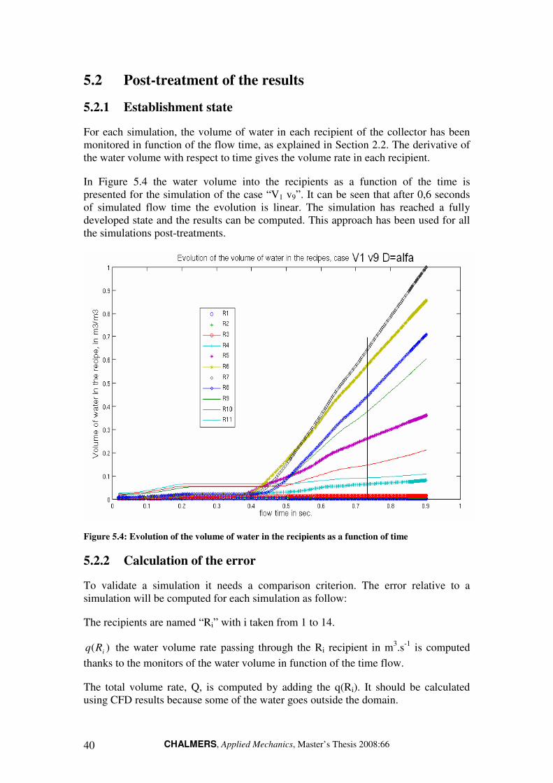
For each simulation, the volume of water in each recipient of the collector has been monitored in function of the flow time, as explained in Section 2.2. The derivative of the water volume with respect to time gives the volume rate in each recipient.

In Figure 5.4 the water volume into the recipients as a function of the time is presented for the simulation of the case “V1 v9”. It can be seen that after 0,6 seconds of simulated flow time the evolution is linear. The simulation has reached a fully developed state and the results can be computed. This approach has been used for all the simulations post-treatments.

Figure 5.4: Evolution of the volume of water in the recipients as a function of time

5.2.2 Calculation of the error

To validate a simulation it needs a comparison criterion. The error relative to a simulation will be computed for each simulation as follow:

The recipients are named “Ri” with i taken from 1 to 14.

)( iRq the water volume rate passing through the Ri recipient in m3.s-1 is computed

thanks to the monitors of the water volume in function of the time flow.

The total volume rate, Q, is computed by adding the q(Ri). It should be calculated using CFD results because some of the water goes outside the domain.


Pexp(Ri) is the fraction of the entire mass flow rate in the Ri recipient is computed for the experiment and for the CFD as follow:

exp

exp

*)()(

Q

SRqRP ii

i = [--] andCFD

iiCFD

iCFDQ

SRqRP

*)()( = . [--]

Pexp(Ri) and PCFD(Ri) are dimensionless and they can be compared. The error for one recipient is expressed as follows:

100*)(

))()(()(

exp

exp

i

iiCFD

iRP

RPRPabsRError

−=

The global error is expressed as follows:

∑=i

i

Q

RiqRErrorError

exp

)(*)(

The global error of a simulation is the mass-weighted averaged of the error in each recipient.


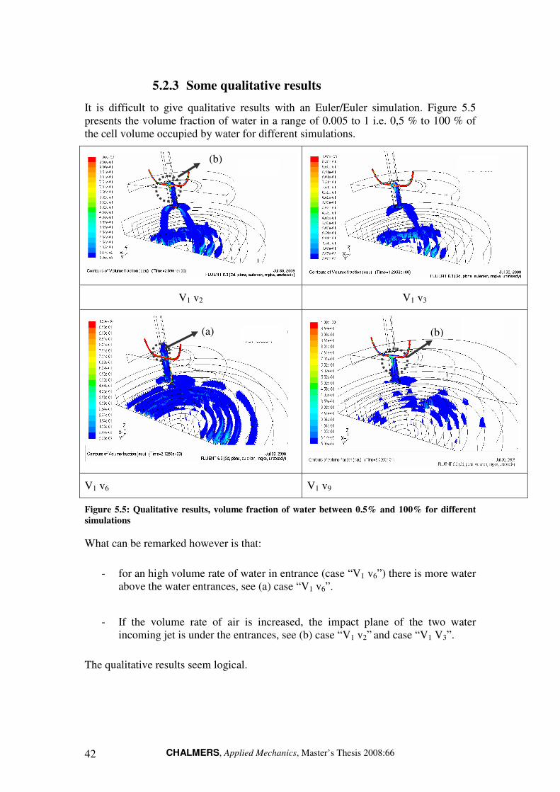
5.2.3 Some qualitative results

It is difficult to give qualitative results with an Euler/Euler simulation. Figure 5.5 presents the volume fraction of water in a range of 0.005 to 1 i.e. 0,5 % to 100 % of the cell volume occupied by water for different simulations.

V1 v2 V1 v3

V1 v6 V1 v9

Figure 5.5: Qualitative results, volume fraction of water between 0.5% and 100% for different

simulations

What can be remarked however is that:

- for an high volume rate of water in entrance (case “V1 v6”) there is more water above the water entrances, see (a) case “V1 v6”.

- If the volume rate of air is increased, the impact plane of the two water incoming jet is under the entrances, see (b) case “V1 v2” and case “V1 V3”.

The qualitative results seem logical.

(a) (b)

(b)


5.3 Quantitative results

5.3.1 Cases We<3

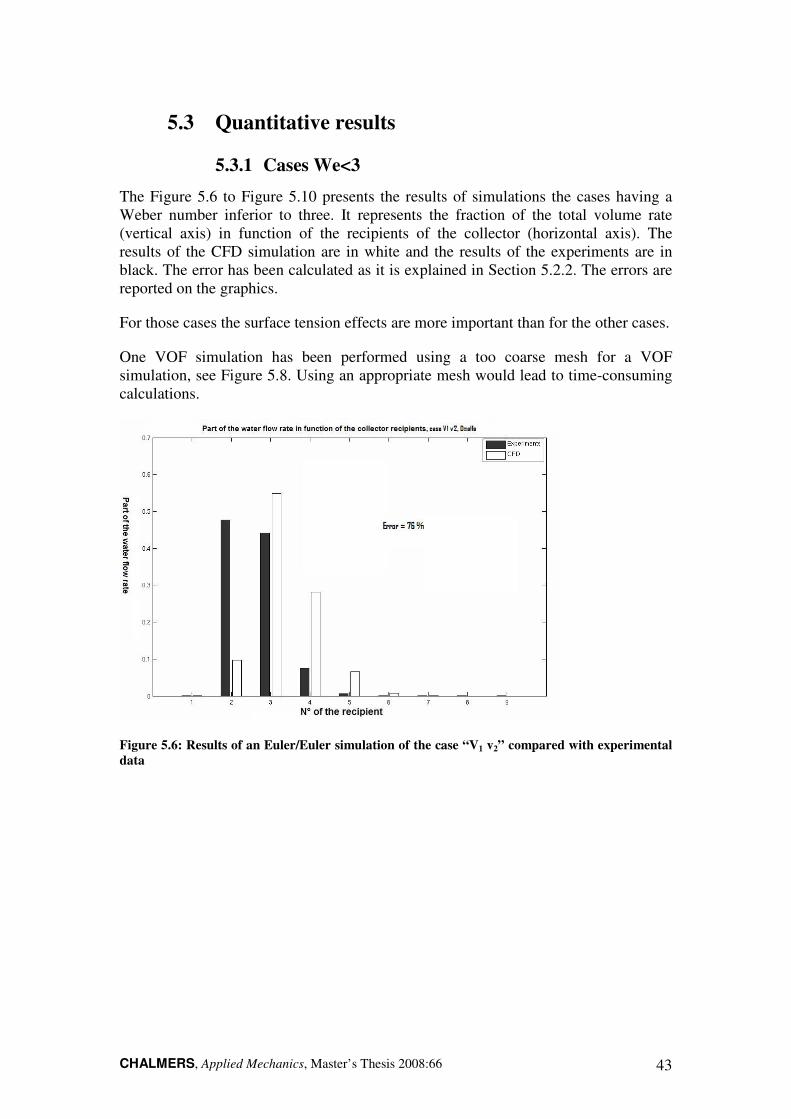
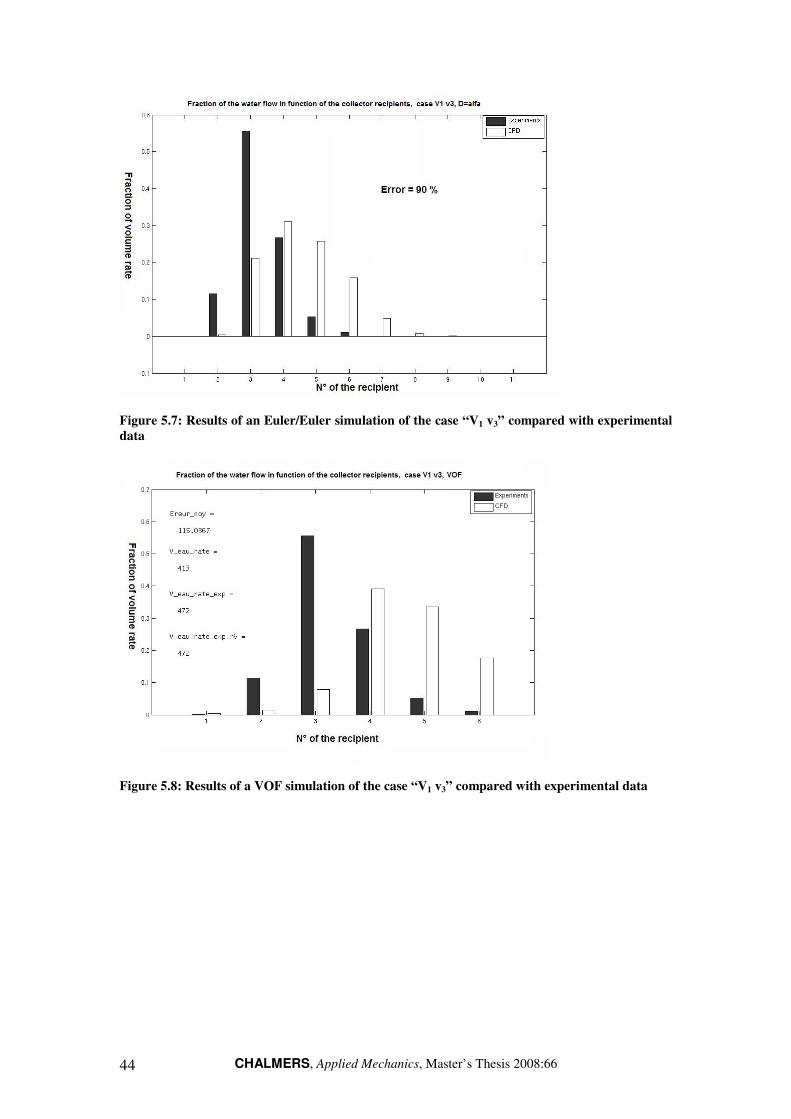
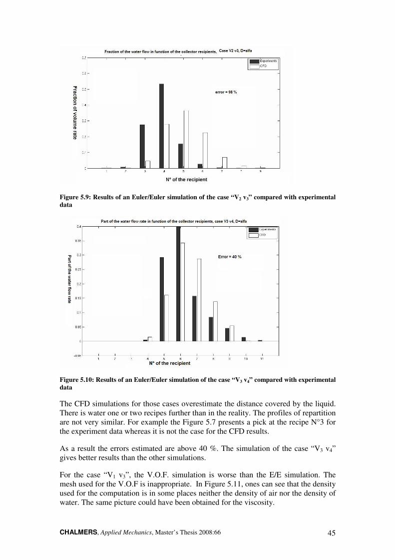
The Figure 5.6 to Figure 5.10 presents the results of simulations the cases having a Weber number inferior to three. It represents the fraction of the total volume rate (vertical axis) in function of the recipients of the collector (horizontal axis). The results of the CFD simulation are in white and the results of the experiments are in black. The error has been calculated as it is explained in Section 5.2.2. The errors are reported on the graphics.

For those cases the surface tension effects are more important than for the other cases.

One VOF simulation has been performed using a too coarse mesh for a VOF simulation, see Figure 5.8. Using an appropriate mesh would lead to time-consuming calculations.

Figure 5.6: Results of an Euler/Euler simulation of the case “V1 v2” compared with experimental

data



data

Figure 5.8: Results of a VOF simulation of the case “V1 v3” compared with experimental data



data


data

The CFD simulations for those cases overestimate the distance covered by the liquid. There is water one or two recipes further than in the reality. The profiles of repartition are not very similar. For example the Figure 5.7 presents a pick at the recipe N°3 for the experiment data whereas it is not the case for the CFD results.

As a result the errors estimated are above 40 %. The simulation of the case “V3 v4” gives better results than the other simulations.

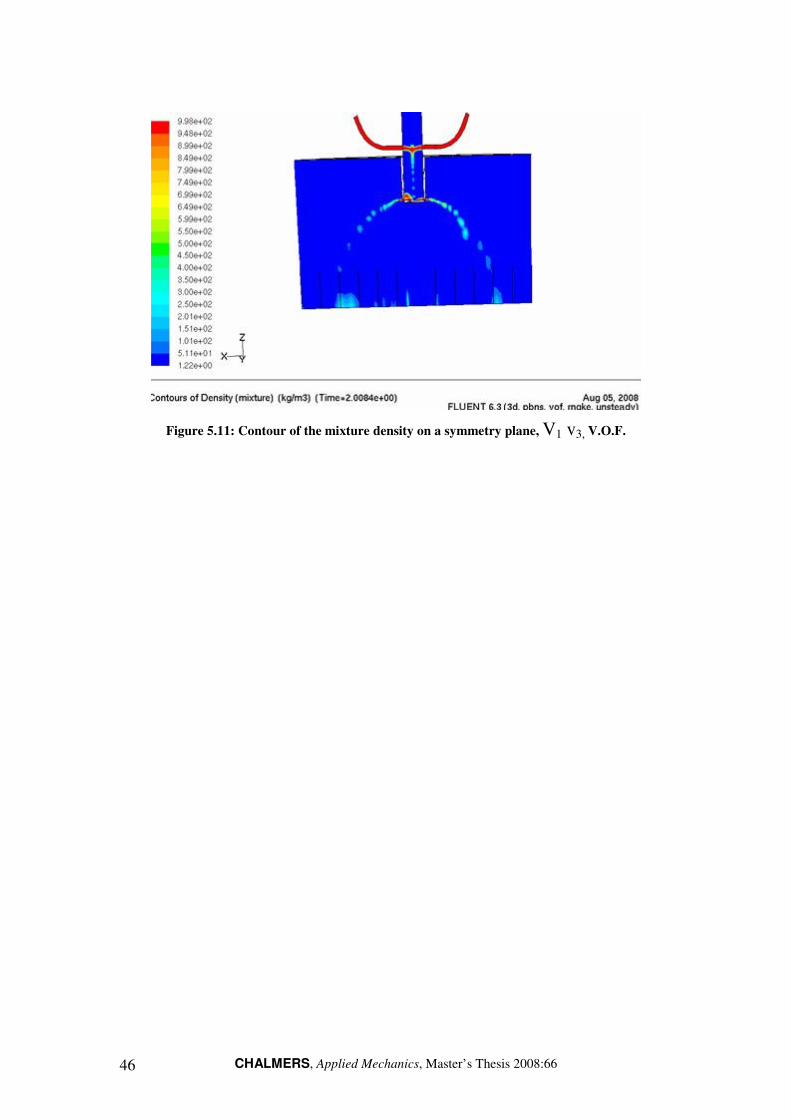
For the case “V1 v3”, the V.O.F. simulation is worse than the E/E simulation. The mesh used for the V.O.F is inappropriate. In Figure 5.11, ones can see that the density used for the computation is in some places neither the density of air nor the density of water. The same picture could have been obtained for the viscosity.


Figure 5.11: Contour of the mixture density on a symmetry plane, V1 v3, V.O.F.


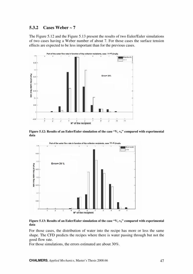
5.3.2 Cases Weber ~ 7

The Figure 5.12 and the Figure 5.13 present the results of two Euler/Euler simulations of two cases having a Weber number of about 7. For those cases the surface tension effects are expected to be less important than for the previous cases.


data


data

For those cases, the distribution of water into the recipe has more or less the same shape. The CFD predicts the recipes where there is water passing through but not the good flow rate. For those simulations, the errors estimated are about 30%.


5.3.3 Cases Weber ~ 27

The Figure 5.14 and the Figure 5.15 present the results of two Euler/Euler simulations of two cases having a Weber number of about 27. For those cases the surface tension effects are expected to be negligible.


data


data

The distribution of water predicted by the CFD simulation is similar to the experimental data. Fore those cases the error is inferior to 16 %. We can say that the CFD is predictive.


Conclusions

The CFD simulations of the flow in a distributor equipped with a deflector leads to the following conclusions:

� The different operating conditions can be classified as function of a Weber number calculated at the interstice between the column and the deflector.

� As expected a VOF simulation of the flow with an inappropriate mesh gives bad results.

� An Euler/Euler simulation with a characteristic droplet length as a setting leads to the following results:

• If We < 3, the CFD overestimates the liquid repartition downstream the distributor

• If We ~ 7, the liquid repartition obtained by CFD is similar to the experimental data, the results could allow a qualitative comparison between different experiments.

• If We ~ 27, the results are in agreement with experimental data. The CFD is predictive.

Before any extrapolation of those results it is important to remark that they are specific for air and water and for a given geometry.


References

Book

Number of the reference Reference

[1] Versteeg & Malalasekera : “An introduction to computational Fluid Dynamics: the final volume method”, edition person, Harlow, England, 1995, 257 pages

Lectures notes


[2] Colin Catherine: « Transferts avec changement de phases », Master « dynamique des fluides, énergétique et transferts » of the fluid mechanics institute of Toulouse, 2006, 100 pages

Notice


[3] Fluent User’s guide for Fluent 6.3.26


Appendices


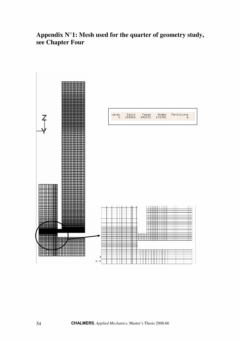
Appendix N°1: Mesh used for the quarter of geometry study,

see Chapter Four

Deflector


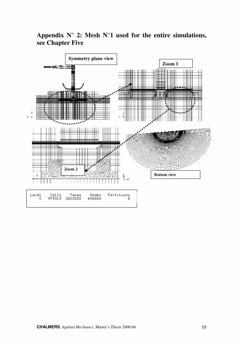
Appendix N° 2: Mesh N°1 used for the entire simulations,

see Chapter Five

Bottom view

Zoom 1

Zoom 2

Symmetry plane view


Appendix N°3: Mesh N°2 used for the entire simulation, see

Chapter Five.

Bottom view

View close to the deflector

CFD simulations of two-phase flows passing through a...

Documents

Transcript of CFD simulations of two-phase flows passing through a...