CFD simulation and analysis of a gas to water two-phase ... · PDF fileThe closest simulation...

CFD simulation and analysis of a gas to water two-phase closed thermosyphon-based heat exchanger

J. B. Ramos1, A. Z. Chong1, C. Tan1, J. Matthews1, M. A. Boocock2 & H. Jouhara2 1Faculty of Advanced Technology, University of South Wales, UK 2Econotherm (UK) Ltd, associate company of Spirax-Sarco Engineering plc, UK

Abstract

Wickless heat pipes are devices with high reliability and heat transfer potential per unit area. Owed to that fact, their application range has been widened in the past 20 years. In the process industry, they are usually coupled to waste heat recovery devices, namely heat exchangers. Heat-pipe-based heat exchangers offer many advantages when compared to conventional waste heat recovery systems, such as increased reliability and reduced cost of production. The design of such devices, however, is not a straightforward process due to the complex modes of heat transfer mechanisms involved. In this paper, the characterisation of a cross-flow heat pipe based heat exchanger is made via the use of ANSYS Fluent, a CFD solver. A design tool with the purpose of predicting the performance of the test unit is also developed and validated through comparison between the CFD model and previous experimental results. Keywords: heat recovery, heat exchangers, heat pipes, thermosyphons, CFD, effectiveness.

1 Introduction

The heat pipe is a heat transfer device with a high heat transfer potential. It consists of a sealed evacuated tube partially filled with a working fluid. The working fluid is responsible for the high heat transfer rates, as a large amount of energy can be transferred via the latent heat in the fluid through phase change.

www.witpress.com, ISSN 1743-3533 (on-line) WIT Transactions on Engineering Sciences, Vol 83, © 2014 WIT Press

Advanced Computational Methods and Experiments in Heat Transfer XIII 217

doi:10.2495/HT140201

Heat pipes have a proven track record in many areas, including space applications [1], computer and electronics [2], ventilation and air conditioning [3, 4], including dehumidification devices [5] heating systems [6, 7], solar energy systems [8], water desalination [9] and nuclear energy [10]; however, waste heat recovery seems to be the preferred application for heat-pipe-equipped heat exchangers [3], partly due to some specific characteristics, namely, the simple structure, high efficiency, compact build, reversibility and the lack of energy input requirement. Heat pipes are physically divided in three sections: the evaporator, located on the lower section of the pipe, where heat is added to the system; the condenser, located on the upper section of the pipe, where heat is removed from it; and the adiabatic section, located between the two. Theoretically, no heat transfer takes place in the adiabatic section. Logically, a heat exchanger equipped with heat pipes can be divided in the same way, the hotter flow used in the lower part (evaporator) and the colder flow used in the upper part (condenser). The basic working principle of a heat pipe consists of a continuous cycle of evaporation/condensation of the working fluid (the name given to the fluid inside the pipe) triggered by a difference in temperature. In the evaporator, the heat supplied to the pipe is absorbed by the working fluid; this triggers the evaporation of the fluid and forces the phase change process, flowing up to the condenser section in a gas form. The wall of the heat pipe is cooler in the condenser section, due to the colder fluid flowing on the shell side. Upon making contact with the cooler surface, the working fluid condenses, giving up its latent heat to the wall of the heat pipe and, due to the force of gravity, flowing back down in a liquid form to the evaporator. There is one characteristic that ought to be mentioned and that is one that substantially alters the behaviour of a heat pipe: the existence (or lack) of a wick structure. The wick usually consists of a sintered structure located on the inside wall of the heat pipe. It applies a capillary pressure to the fluid, allowing it to flow towards the evaporator even when turned upside down and against the force of gravity. Wickless heat pipes are technically named two-phase closed thermosyphons or gravity-assisted heat pipes and are the type used in this paper.

1.1 Literature

Heat pipes have been thoroughly investigated in the past decade [11]. However, due to the intricacies in simulating the phase change process inside the pipe, there are only a handful of Computational Fluid Dynamics (CFD) simulation studies available on the topic and most of them two dimensional. More so, most of the studies were done at temperatures below 50ºC, as the researchers often aim at studying the application of heat pipes in refrigeration or air conditioner units. For the sake of comparison, in industrial waste heat recovery, the temperature of an exhaust can rise to 300ºC and the pipes usually have more than 2 metres length. The closest simulation of the two-phase flow within a heat pipe has been developed by Fadhl et al. [12]. In his two dimensional study, he was able to


218 Advanced Computational Methods and Experiments in Heat Transfer XIII

accurately simulate the actual boiling and condensation processes inside the pipe through user-defined functions using the Volume of Fluid (VoF) method in ANSYS FLUENT. However, simulating the phase change process, even in a two-dimensional study is not an easy matter, and that is the main reason the VoF method is not yet widely used to simulate bundles of pipes or heat pipe-equipped heat exchangers. Instead, most recent papers treat the heat pipe as a single entity, as Annamalai and Ramalingam [13] did when investigating a wicked heat pipe; in an effort to create a better correlation, who chose not to simulate the evaporation and boiling processes inside the pipe, assuming the inner side of the pipe to be composed of a single phase of vapour and the wick structure to be a liquid phase throughout the inner wall of the pipe. Good agreement was found between the predicted surface temperature and the experimental results. Legierski et al. [14] also conducted a study in a horizontal wicked heat pipe in a low temperature environment (< 100ºC). The variation of thermal conductivity through time was investigated, and the simulation, once again, proved to be very close to the experimental results. The thermal conductivity of the pipe was estimated to range between 15,000 and 30,000 W/m K, a value achieved after 20–30 seconds of operation. So it is possible to have good agreement between a CFD study and experimental data without simulating the two-phase flow. There are even applications within the CFD solver that allow the user to simulate the heat exchanger; in fact, Drosatos et al. [15] have used this macro heat exchanger approach in their heat pipe based heat exchanger experiments and achieved very accurate sets of data. The working fluid outlet temperatures and the conjugated heat flux deviated by less than 3.6% and 5.7%, respectively. In addition, CFD simulation can also be used in order to increase the performance of an existing heat exchanger, even when equipped with heat pipes, as has been proven by Selma et al. [17]. The improvement in performance resulting from changes in the pipe diameter and the angle between the pipes was investigated within the CFD simulation and then applied to the heat exchanger under investigation. The limitations seem to always be the same, a limited temperature range that does not take into account waste heat applications (0–40ºC). The present paper produces a CFD simulation predicting the heat transfer performance of a heat exchanger equipped with heat pipes, assuming the heat pipes are solid materials with a constant thermal conductivity. The advantage of this method is a lower simulation time and high adaptability, with possibility of being used in other heat exchanger designs equipped with heat pipes. The numerical model presented in this paper is a replica of a real heat exchanger used in an experimental rig that was built with the purpose of investigating the behaviour of an actual air-to-water heat exchanger equipped with heat pipes. The model predictions are then compared to the experimental results in an effort to prove the new method (using a constant conductivity) has the potential to size heat pipe based heat exchangers operating at higher temperatures.



2 Physical problem description

The heat exchanger being simulated in this paper is based on an experimental rig that aimed at characterising an air-to-water heat pipe based heat exchanger. In Figure 1 the heat exchanger can be seen rotated 90º to the right. As can be observed, the three sections are clearly shown, the evaporator (0.6 m on the left), the condenser (0.2 m on the right) and the adiabatic section composing the sections in the middle. The thermocouples were placed in key locations, namely in all the inlets and outlets and on the surface of the pipes at 0.6 m intervals.

Figure 1: Representative schematic of the heat pipe heat exchanger and respective thermocouple locations (represented by the circles). The evaporator is located on the left and the evaporator on the right.

The heat exchanger is equipped with a set of 6 vertical heat pipes in a staggered arrangement. The pipes are two-phase closed thermosyphons measuring 2.0 m and having a diameter of 28.0 mm. The pipes are made of carbon steel, filled with distilled water to about a third of their total length. The surrounding wall of the heat pipes has an average thickness of 2.5 mm. In the evaporator section, the pipes are swept 3 at a time by the hot air (looking at Figure 2, the hot air flows from the bottom to the top of the picture). In the condenser, the pipes are swept as shown in Figure 2. Following the arrows, the flow takes a u-turn, sweeping the pipes in order.

Figure 2: Cross-section of the Condenser part of the Heat Exchanger (top view all dimensions in mm).



The principal purpose of this simulation is to prove that by equating the heat pipe to a solid rod of constant conductivity, the other modes of heat transfer inside the heat pipe can be neglected. The temperature and mass flow rate of hot incoming air varied from 50ºC to 300ºC and 0.05 kg/s to 0.2 kg/s, respectively. The water inlet was kept at a constant mass flow rate of 0.07 kg/s and constant temperature at 10ºC.

2.1 Numerical model

ANSYS Fluent was used to develop a numerical model to simulate the external heat flow over the pipes on both the air side (evaporator) and water side (condenser). The model was developed in order to access the possibility of using constant conductivity as a boundary condition in heat pipe simulation for future heat exchanger modelling. The mesh was first built and sized. Afterwards, the full range of simulations attempted the repetition of the experimental results and finally the results were compared with the experimental results. The standard k-epsilon (k-ε) turbulence model was used for all the tested results. It is the most used model in practical engineering flow calculations due to its robustness and reasonable accuracy for a wide range of turbulent flows. It is a semi-empirical model based on model transport equations for the turbulence kinetic energy (k) and its dissipation rate (ε). In order to use the standard k-ε, the flow has to be fully turbulent. The pressure-velocity scheme used was coupled as it offers a better result for a single-phase flow, more consistent and efficient at steady-state [16]. This is due to the fact that the algorithm solves the pressure-based continuity and momentum equations simultaneously.

2.2 Mesh selection

There were three meshing levels generated: coarse, medium and fine. In the case of hexahedrons or tetrahedrons meshes, the maximum skewness should be lower than 0.7, while in triangular elements, it must be inferior to 0.8 [17].

Table 1: Mesh dependency.

Level No of Cells Type of cells Max. Skewness Time/iter (s) Coarse 191,299 Hex + Tetra 0.68 0.5–1 Medium 825,904 Hex + Tetra 0.70 10–12 Fine 1,518,970 Hex + Tetra 0.57 24–26

Two evaporator inlet conditions were considered to which the experimental results were compared to the simulated results. The results provided by the fine mesh were the most acceptable in the end and the limit guaranteed for grid independency. The medium mesh gave unexpected results, less accurate than the experimental.



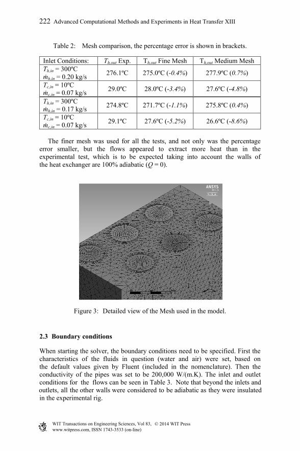
Table 2: Mesh comparison, the percentage error is shown in brackets.

Inlet Conditions: Th,out Exp. Th,out Fine Mesh Th,out Medium Mesh Th,in = 300ºC ṁh,in = 0.20 kg/s 276.1ºC 275.0ºC (-0.4%) 277.9ºC (0.7%)

Tc,in = 10ºC ṁc,in = 0.07 kg/s 29.0ºC 28.0ºC (-3.4%) 27.6ºC (-4.8%)

Th,in = 300ºC ṁh,in = 0.17 kg/s 274.8ºC 271.7ºC (-1.1%) 275.8ºC (0.4%)

Tc,in = 10ºC ṁc,in = 0.07 kg/s 29.1ºC 27.6ºC (-5.2%) 26.6ºC (-8.6%)

The finer mesh was used for all the tests, and not only was the percentage error smaller, but the flows appeared to extract more heat than in the experimental test, which is to be expected taking into account the walls of the heat exchanger are 100% adiabatic (Q = 0).

Figure 3: Detailed view of the Mesh used in the model.

2.3 Boundary conditions

When starting the solver, the boundary conditions need to be specified. First the characteristics of the fluids in question (water and air) were set, based on the default values given by Fluent (included in the nomenclature). Then the conductivity of the pipes was set to be 200,000 W/(m.K). The inlet and outlet conditions for the flows can be seen in Table 3. Note that beyond the inlets and outlets, all the other walls were considered to be adiabatic as they were insulatedin the experimental rig.



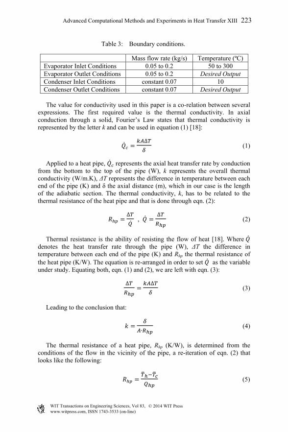
Table 3: Boundary conditions.

Mass flow rate (kg/s) Temperature (ºC) Evaporator Inlet Conditions 0.05 to 0.2 50 to 300 Evaporator Outlet Conditions 0.05 to 0.2 Desired Output Condenser Inlet Conditions constant 0.07 10 Condenser Outlet Conditions constant 0.07 Desired Output

The value for conductivity used in this paper is a co-relation between several expressions. The first required value is the thermal conductivity. In axial conduction through a solid, Fourier’s Law states that thermal conductivity is represented by the letter k and can be used in equation (1) [18]:

�̇�𝑐 = 𝑘𝐴∆𝑇𝛿

(1) Applied to a heat pipe, �̇�𝑐 represents the axial heat transfer rate by conduction from the bottom to the top of the pipe (W), k represents the overall thermal conductivity (W/m.K), ΔT represents the difference in temperature between each end of the pipe (K) and δ the axial distance (m), which in our case is the length of the adiabatic section. The thermal conductivity, k, has to be related to the thermal resistance of the heat pipe and that is done through eqn. (2):

𝑅ℎ𝑝 = ∆𝑇�̇�

, �̇� = ∆𝑇𝑅ℎ𝑝

(2)

Thermal resistance is the ability of resisting the flow of heat [18]. Where �̇� denotes the heat transfer rate through the pipe (W), ΔT the difference in temperature between each end of the pipe (K) and Rhp the thermal resistance of the heat pipe (K/W). The equation is re-arranged in order to set �̇� as the variable under study. Equating both, eqn. (1) and (2), we are left with eqn. (3):

∆𝑇𝑅ℎ𝑝

= 𝑘𝐴∆𝑇𝛿

(3) Leading to the conclusion that:

𝑘 = 𝛿

𝐴∙𝑅ℎ𝑝 (4)

The thermal resistance of a heat pipe, Rhp (K/W), is determined from the conditions of the flow in the vicinity of the pipe, a re-iteration of eqn. (2) that looks like the following:

𝑅ℎ𝑝 = 𝑇�ℎ−𝑇�𝑐𝑄ℎ𝑝

(5)



𝑇�𝑐 and 𝑇�ℎ represent the average temperature in both the evaporator and the condenser sections (K) and Qhp is the heat flow through the heat pipe (W). Since the heat exchanger is equipped with 6 heat pipes, the use of the Total Resistance, RT (K/W), is advised. Following the electric circuit analogy, the heat pipes are assumed to be thermal resistances arranged in parallel and the Total Thermal Resistance becomes the following:

𝑅𝑇 = 1

1𝑅ℎ𝑝1

+ 1𝑅ℎ𝑝2

+ 1𝑅ℎ𝑝3

+ 1𝑅ℎ𝑝4

+ 1𝑅ℎ𝑝5

+ 1𝑅ℎ𝑝6

(6)

Assuming all the heat pipes offer the same resistance to heat transfer:

𝑅𝑇 =𝑅ℎ𝑝𝑛

(7) where n represents the number of heat pipes in the heat exchanger. The total resistance is related to the heat flow of the entire heat exchanger through equation (2), which leads to the determination of Rhp which in turn allows the calculation of k as a boundary condition in the CFD simulation.

3 Results and discussion

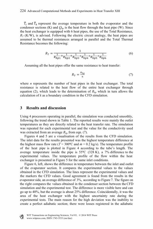
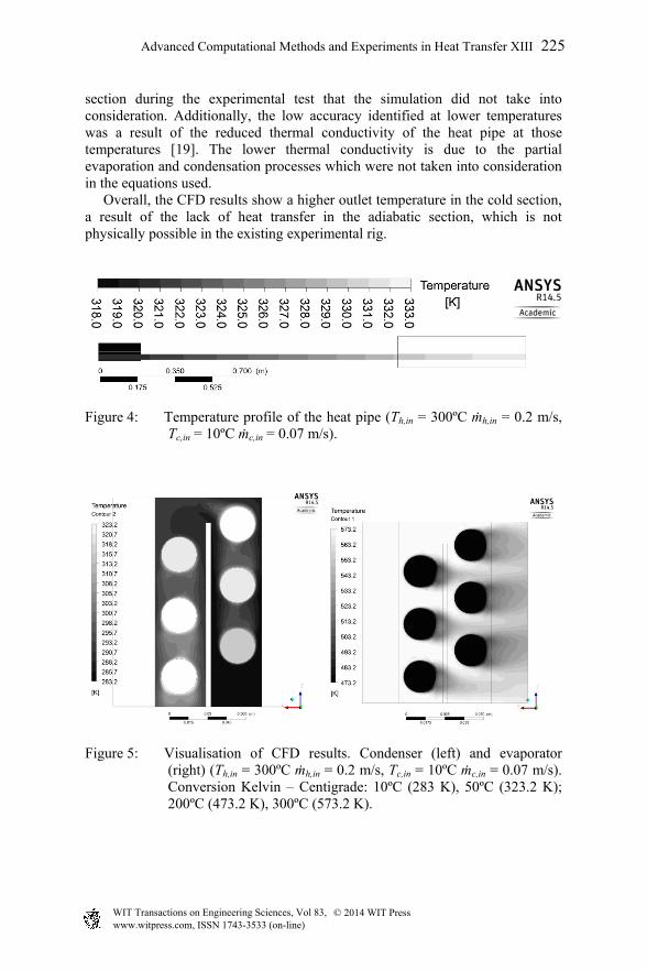
Using 4 processors operating in parallel, the simulation was conducted smoothly, following the trend shown in Table 1. The reported results were mainly the outlet temperatures as they are directly related to the heat transfer rate. The simulation was repeated for each experimental test and the value for the conductivity used was extracted from an average Rhp from eqn. (7). Figures 4 and 5 are a visualisation of the results from the CFD simulation. The inlet data for the results presented was the highest temperature difference at the highest mass flow rate (T = 300ºC and ṁ = 0.2 kg/s). The temperature profile of the heat pipe is plotted in Figure 4 according to the tube’s length. The average temperature inside the pipe is 55ºC (328 K), a 7% difference to the experimental values. The temperature profile of the flow within the heat exchanger is presented in Figure 5 for the same inlet conditions. Figure 6, left, shows the difference in temperature between the inlet and outlet of the evaporator section. It compares the experimental values to the values obtained in the CFD simulation. The lines represent the experimental values and the markers the CFD values. Good agreement is found from the results in the evaporator side, an average difference of 3%, according to Figure 7. The figure on the right compares the values obtained in the condenser section between the CFD simulation and the experimental test. The difference is more visible here and can go up to 40%, but the average is about 25% difference. Coincidentally, it was the area of the heat exchanger with the highest uncertainty rate during the experimental tests. The main reason for the high deviation was the inability to create a perfect adiabatic section; there were losses registered in the adiabatic



section during the experimental test that the simulation did not take into consideration. Additionally, the low accuracy identified at lower temperatures was a result of the reduced thermal conductivity of the heat pipe at those temperatures [19]. The lower thermal conductivity is due to the partial evaporation and condensation processes which were not taken into consideration in the equations used. Overall, the CFD results show a higher outlet temperature in the cold section, a result of the lack of heat transfer in the adiabatic section, which is not physically possible in the existing experimental rig.

Figure 4: Temperature profile of the heat pipe (Th,in = 300ºC ṁh,in = 0.2 m/s, Tc,in = 10ºC ṁc,in = 0.07 m/s).

Figure 5: Visualisation of CFD results. Condenser (left) and evaporator (right) (Th,in = 300ºC ṁh,in = 0.2 m/s, Tc,in = 10ºC ṁc,in = 0.07 m/s). Conversion Kelvin – Centigrade: 10ºC (283 K), 50ºC (323.2 K); 200ºC (473.2 K), 300ºC (573.2 K).



Figure 6: Difference in temperature in the evaporator and condenser sections.

Figure 7: Percentage difference between outlet temperatures in the condenser section.

4 Conclusion

CFD has been used to simulate the behaviour of a heat pipe based heat exchanger through the assumption that the heat pipes are solid devices of constant conductivity. The model results proved to be within an average of 20% of the experimental results assuming a constant conductivity for all the results. The creation of a relation between thermal resistance of the heat pipe and inlet conditions is suggested in order to perfect the model.

Acknowledgements

Special thanks are due to Mr. Stefan Munteanu and to Mr. Peter Blackwell for the fast and flawless way the experimental rig was prepared. Thanks are also due to Mr. David Jenkins, Mr. Hassan Mroue and Mr. Michael Jones for their overall helpfulness.

0

50

100

150

200

250

300

0 10 20 30 40 50 60

Ti-T

o Eva

p. (o C

)

Frequency of Fan (Hz)

5

10

15

20

25

30

35

0 10 20 30 40 50 60

To-

Ti C

ond.

(o C)


0%

1%

2%

3%

4%

5%

6%

7%

0 10 20 30 40 50 60

%di

ff. C

FD/e

xp.


0%

10%

20%

30%

40%

0 10 20 30 40 50 60

%di

ff. C

FD/e

xp.




Nomenclature

A (m2) Heat Transfer Area k (W/(m.K)) Constant of Thermal Conductivity ṁ (kg/s) Mass Flow Rate �̇� (W) Heat Transfer Rate R (K/W) Thermal Resistance T (oC) Temperature 𝑇� (oC) Average Temperature ΔT (oC) Difference in Temperature U (W/(m2.K)) Overall Heat Transfer Coefficient δ (m) Distance (used in Conduction) Ɛ (-) Effectiveness

Subscripts c Condenser side/Cold side h / e Hot side/Evaporator side hp Heat pipe/Thermosyphon i Inlet n Number of pipes o Outlet T Total w Water Abbreviations CFD Computational Fluid Dynamics HPHE Heat pipe Heat Exchanger k-ε k-epsilon turbulence method NTU Number of Transfer Units VoF Volume of Fraction

References

[1] Dong, S.J., Li, Y.Z. & Wang, J., Fuzzy incremental control algorithm of loop heat pipe cooling system for spacecraft applications, Computers & Mathematics with Applications, 64 (2012) 877-886.

[2] Wang, J.C., 3-D numerical and experimental models for flat and embedded heat pipes applied in high-end VGA card cooling system, International Communications in Heat and Mass Transfer, 39 (2012) 1360-1366.

[3] Jouhara, H. & Robinson, A.J., An experimental study of small-diameter wickless heat pipes operating in the temperature range 200C to 450C., Applied Thermal Engineering, 30 (2011) 1041-1048.



[4] Chaudhry, H.N., Hughes, B.R. & Ghani S.A., A review of heat pipe systems for heat recovery and renewable energy applications, Renewable and Sustainable Energy Reviews, 16 (2012) 2249-2259.

[5] Yau, Y.H. & Ahmadzadehtalatapeh, M., A review on the application of horizontal heat pipe heat exchangers in air conditioning systems in the tropics, Applied Thermal Engineering, 30 (2010) 77-84.

[6] Wang, Z., Duan, Z., Zhao, X., & Chen, M., Dynamic performance of a façade-based solar loop heat pipe water heating system, Solar Energy, 86 (2012) 1632-1647.

[7] Zhang, X., Zhao, X., Xu, J. & Yu, X., Characterization of a solar photovoltaic/loop-heat-pipe heat pump water heating system, Applied Energy, 102 (2013) 1229-1245.

[8] Nithyanandam K. & Pitchumani, R., Computational studies on a latent thermal energy storage system with integral heat pipes for concentrating solar power, Applied Energy, 103 (2013) 400-415.

[9] Jouhara, H., Anastasov, V. & Khamis, I., Potential of heat pipe technology in nuclear seawater desalination, Desalination, 249 (2009) 1055-1061.

[10] Laubscher, R. & Dobson, R.T., Theoretical and experimental modelling of a heat pipe heat exchanger for high temperature nuclear reactor technology, Applied Thermal Engineering, 61 (2013) 259-267.

[11] Vasiliev, L.L., Heat pipes in modern heat exchangers, Applied Thermal Engineering, 25 (2005) 1-19.

[12] Fadhl, B., Wrobel, L.C. & Jouhara, H., Numerical modelling of the temperature distribution in a two-phase closed thermosyphon, Applied Thermal Engineering, 60 (2013) 122-131.

[13] Annamalai, A. & Ramalingam, V., Experimental Investigation and Computational Fluid Dynamics of a Air Cooled Condenser Heat Pipe, Thermal Science, 15 (2011) 759-772.

[14] Legierski, J., Wieçek, B. & de Mey, G., Measurements and simulations of transient characteristics of heat pipes, Microelectronics Reliability, 46 (2006) 109-115.

[15] Drosatos, P., Nikolopoulos, N., Agraniotis, M., Itskos, G., Grammelis, P. & Kakaras, E., Decoupled CFD simulation of furnace and heat exchangers in a lignite utility boiler, Fuel, 117, Part A (2014) 633-648.

[16] FLUENT 6.3 Us er’s Gu ide, Fl uent Inc . Online: http://aerojet.engr.ucdavis.edu/fluenthelp/html/ug/node998.htm

[17] Selma, B., Désilets, M. & Proulx, P., Optimization of an industrial heat exchanger using an open-source CFD code, Applied Thermal Engineering, (2013).

[18] Incropera, F. & Dewitt, D., Fundamentals Of Heat And Mass Transfer, 4th Ed, John Wiley & Sons, 1996.

[19] Khazaee, I, Hosseini, R. & Noie, S.H., Experimental investigation of effective parameters and correlation of geyser boiling in a two-phase closed thermosyphon, Applied Thermal Engineering, (2010).



CFD simulation and analysis of a gas to water two-phase ... · PDF fileThe closest simulation...

Documents

Transcript of CFD simulation and analysis of a gas to water two-phase ... · PDF fileThe closest simulation...