CFD Performance of Turbulence Models for Flow from ...

Washington University in St. Louis Washington University in St. Louis

Washington University Open Scholarship Washington University Open Scholarship

Engineering and Applied Science Theses & Dissertations McKelvey School of Engineering

Summer 8-17-2017

CFD Performance of Turbulence Models for Flow from Supersonic CFD Performance of Turbulence Models for Flow from Supersonic

Nozzle Exhausts Nozzle Exhausts

Han Ju Lee Washington University in St. Louis

Follow this and additional works at: https://openscholarship.wustl.edu/eng_etds

Part of the Engineering Commons

Recommended Citation Recommended Citation Lee, Han Ju, "CFD Performance of Turbulence Models for Flow from Supersonic Nozzle Exhausts" (2017). Engineering and Applied Science Theses & Dissertations. 260. https://openscholarship.wustl.edu/eng_etds/260

This Thesis is brought to you for free and open access by the McKelvey School of Engineering at Washington University Open Scholarship. It has been accepted for inclusion in Engineering and Applied Science Theses & Dissertations by an authorized administrator of Washington University Open Scholarship. For more information, please contact [email protected].

https://openscholarship.wustl.edu/

https://openscholarship.wustl.edu/eng_etds

https://openscholarship.wustl.edu/eng_etds

https://openscholarship.wustl.edu/eng

https://openscholarship.wustl.edu/eng_etds?utm_source=openscholarship.wustl.edu%2Feng_etds%2F260&utm_medium=PDF&utm_campaign=PDFCoverPages

http://network.bepress.com/hgg/discipline/217?utm_source=openscholarship.wustl.edu%2Feng_etds%2F260&utm_medium=PDF&utm_campaign=PDFCoverPages

https://openscholarship.wustl.edu/eng_etds/260?utm_source=openscholarship.wustl.edu%2Feng_etds%2F260&utm_medium=PDF&utm_campaign=PDFCoverPages

mailto:[email protected]

WASHINGTON UNIVERSITY IN ST. LOUIS

School of Engineering and Applied Science

Department of Mechanical Engineering and Materials Science

Thesis Examination Committee:

Ramesh K. Agarwal, Chair

Qiulin Qu

Mark Meacham

CFD Performance of Turbulence Models for Flow from Supersonic Nozzle Exhausts

A Thesis presented to

the School of Engineering &

Applied Science of Washington University in

partial fulfillment of the

requirements for the degree

of Master of Science

August 2017

St. Louis, Missouri

ii

Table of Contents List of Figures ................................................................................................................................ iv

List of Tables ................................................................................................................................. vi

Acknowledgments......................................................................................................................... vii

ABSTRACT OF THE THESIS ..................................................................................................... ix

Chapter 1 Introduction ............................................................................................................... 1

Chapter 2 Turbulence Models ................................................................................................... 3

2.1 Shear Stress Transport k-ω Model ............................................................... 3

2.2 Spalart-Allmaras Model ............................................................................... 4

2.3 Wray-Agarwal Model .................................................................................. 5

2.4 Standard k-ε Model ...................................................................................... 6

2.5 Yang-Shih Low Reynolds Number k-ε Model ............................................. 7

Chapter 3 Compressibility Correction ....................................................................................... 9

3.1 Compressibility Correction for k-ε Models .................................................. 9

3.2 Compressibility Correction for SST k-ω model ........................................ 11

3.3 Compressibility Correction for WA Model ............................................... 12

Chapter 4 Supersonic Nozzle Exhaust Test Cases .................................................................. 15

4.1 Putnam Nozzle ........................................................................................... 15

4.2 Seiner Nozzle ............................................................................................. 15

4.3 Eggers Nozzle ............................................................................................ 16

Chapter 5 Results and Discussion ........................................................................................... 18

5.1 Grid Generation, Solver Specification and Convergence .......................... 18

5.2 Putnam Nozzle Results .............................................................................. 20

5.3 Seiner Nozzle Results ................................................................................ 24

5.3.1 Results without Compressibility Correction .............................................. 24

5.3.2 Results with Compressibility Correction for k-ε and SST k-ω Models ..... 28

5.3.3 Results with Compressibility Correction for Wray-Agarwal Model ......... 33

5.4 Eggers Nozzle Results ............................................................................... 34

iii

5.4.1 Results without Compressibility Correction .............................................. 35

5.4.2 Results with Compressibility Correction SST k-ω, k-ε and Low Reynolds

Number k-ε Models ..................................................................................................... 39

5.4.3 Results with Compressibility Correction for WA Model .......................... 45

Chapter 6 Conclusions ............................................................................................................. 49

Chapter 7 References ............................................................................................................... 51

Vita ................................................................................................................................................ 53

iv

List of Figures Fig. 1 Putnam nozzle geometry from Ref. [2]. ............................................................................. 16

Fig. 2: Seiner nozzle geometry from Ref. [16]. ............................................................................ 16

Figure 3 Eggers nozzle geometry from Ref. [20] ......................................................................... 17

Figure 4 Original and adapted grids for the Putnam nozzle. ........................................................ 19

Figure 5 Original and adapted grids for the Seiner nozzle. .......................................................... 19

Figure 6 Original and Adapted grids for Eggers Nozzle .............................................................. 20

Figure 7 Variation in Pressure ΔP/P0 along the axis at a distance 15.24 cm above the centerline

of Putnam nozzle........................................................................................................................... 21

Figure 8 Variation in Mach number along the axis at a distance 15.24 cm above the centerline of

Putnam nozzle. .............................................................................................................................. 21

Figure 9 Mach contours in Putnam nozzle exhaust using the SST k-ω model. ............................ 22

Figure 10 Zoomed-in Mach contours in Putnam nozzle exhaust using SST k-ω model. ............. 22

Figure 11 Pressure contours in Putnam nozzle exhaust using SST k-ω model. ........................... 23

Figure 12 Zoomed-in pressure contours in Putnam nozzle exhaust using SST k-ω model. ......... 23

Figure 13 Variation in Mach number along the centerline from the jet exit for Seiner nozzle

using various standard baseline turbulence models. ..................................................................... 25

Figure 14 Mach contours in Seiner nozzle exhaust using SST k-w model. .................................. 26

Figure 15 Zoomed-in Mach contours in Seiner nozzle exhaust using SST k-w model. ............... 26

Figure 16 Pressure contours in Seiner nozzle exhaust using SST k-w model. ............................ 27

Figure 17 Zoomed-in pressure contours in Seiner nozzle exhaust using SST k-w model. ........... 27


using various standard turbulence models with Sarkar’s compressibility correction. .................. 28


using k- ε model with various values of α1 in Sarkar’s compressibility correction. ..................... 29


using different low Reynolds number k- ε models with and without Sarkar’s compressibility

correction. ..................................................................................................................................... 31

Figure 21 Comparison of Skin Friction coefficient on the wall of Seiner nozzle using various

versions of k- ε models with and without Sarkar’s compressibility correction; x = 0 is the jet

exit................................................................................................................................................. 32


using Wray-Agarwal model with Sarkar’s compressibility correction. ........................................ 34

Figure 23 Variation in u/u_exit along the centerline from the jet exit for Eggers nozzle using

various baseline turbulence models without compressibility correction. ..................................... 36

Figure 24 Variation in u/u_exit along the radial direction at x/r_exit=3.06 for Eggers nozzle

using various baseline turbulence models without compressibility correction. ........................... 37



v






various turbulence models with and without Sarkar’s compressibility correction. ...................... 41


using k-ε, low Reynold number k-ε turbulence model and SA models with and without Sarkar’s

compressibility correction. ............................................................................................................ 41


using SST k-ω and Wray-Agarwal turbulence models with and without compressibility

correction. ..................................................................................................................................... 42






correction. ..................................................................................................................................... 43






correction. ..................................................................................................................................... 44


using k-ε, low Reynold number k-ε turbulence model and SA models with and without Sarkar




correction. ..................................................................................................................................... 45


Wray-Agarwal turbulence models with two different compressibility corrections. ..................... 47


using Wray-Agarwal turbulence models with two different compressibility corrections. ........... 47





vi

List of Tables Table 1 Nozzle internal coordinates for Eggers nozzle [20]......................................................... 17

vii

Acknowledgments This Master’s thesis represents how I have grown to be a scientist and what I have

learned through my research experience at Washington University in St. Louis. This place has

allowed me to learn and share ideas with one of the most brilliant group of people I have ever

known. I would like to use this opportunity to express gratitude to all the people who have

guided and supported me throughout 5 years I have spent at Washington University in St. Louis.

First, I would like to thank my advisor, Dr. Agarwal, for his helpful guidance,

encouragement and deep knowledge. It would have taken me much longer time and effort to

finish this research without him. Moreover, I thank him for making thoughtful comments to

improve this manuscript as well. This thesis would have lacked in many ways without him.

Moreover, it was Tim Wray’s expertise in ANSYS programs and research methods that

gave the momentum to my research. Tim taught me how to use ANSYS programs and solved

many problems that I could not have solved. I am also grateful for the long hours he spent to

teach me every single detail needed for research, from what to do when certain errors occur to

what to check to create a sound mesh. I wish him the best as he starts his scholastic journey this

year after finishing PhD under Dr. Agarwal.

Last but not least, I am indebted to my parents for their financial as well as emotional

support for my entire academic career. My father’s useful advice in deciding which path to

follow as well as my mother’s heartwarming letters strengthened me to plow through difficult

times during my academic career.

Washington University in St. Louis Han Ju Lee

August 2017

viii

Dedicated to my parents, Chang Lyoul Lee and Kyoung Sook Kim.

ix

ABSTRACT OF THE THESIS

CFD Performance of Turbulence Models for Flow from Supersonic Nozzle Exhausts

by

Han Ju Lee

Master of Science in Aerospace Engineering

Washington University in St. Louis, 2017

Research Advisor: Professor Ramesh K. Agarwal

The goal of this thesis is to compare the performance of several eddy-viscosity turbulence

models for computing supersonic nozzle exhaust flows. These flows are of relevance in the

development of future supersonic transport airplane. Flow simulations of exhaust flows from

three supersonic nozzles are computed using ANSYS Fluent. Simulation results are compared to

experimental data to assess the performance of various one- and two-equation turbulence models

for accurately predicting the supersonic plume flow. One particular turbulence model of interest

is the Wray-Agarwal (WA) turbulence model. This is a neat model which has demonstrated

promising results mimicking the strength of two equation k-ω model while being a one equation

model. Compressibility corrections are implemented for CFD simulations with SST k-ω, k-ε and

low Reynolds versions of k-ε models which improved the results compared to the baseline

models without compressibility correction. A compressibility correction for WA model is also

developed to compare the performance of a compressibility correction to WA model with the

compressibility correction to other models. Results show that the standard eddy-viscosity models

can capture the shock structure and shear layer of the plume accurately when the thickness of the

shear layer is small compared to plume diameter. However, when thickness of the shear layer is

relatively large, a compressibility correction should be implemented to predict the supersonic jet

x

flow. However, the use of compressibility correction consistently overestimates the length of

potential core on the centerline of the plume although it improves the prediction of the velocity

profile in other regions of the flow field such as the mixing region. Also, it is speculated that an

accurate prediction of boundary layer profile at the nozzle exit has an influence in the model’s

ability to predict the length of potential core as well as the shear layer growth rate. No single

model appears to capture all features of the plumes’ flow fields without or with compressibility

correction. In particular, WA model shows an excellent potential for computation of supersonic

nozzles’ exhaust flows; however further improvements and investigations in WA model are

warranted.

1

Chapter 1

Introduction Accurate prediction of engine exhaust plumes from supersonic nozzles using

computational fluid dynamics (CFD) software has become a topic of great interest in recent years

because of its relevance in the development of future supersonic transport airplanes. This renewed

interest in supersonic flight can also be noticed in the outcomes of AIAA Sonic Boom Prediction

Workshop [1], where numerous codes have been applied to predict the sonic booms of several

model supersonic bodies to test their prediction capability. However, there have been limited

investigations of the effect of the engine plume on the boom signature and the supersonic flight

vehicle. The goal of this thesis is to partially address this problem by studying the plume flow from

supersonic nozzles by numerical simulation. The particular focus is on assessing the performance

of several widely used eddy-viscosity turbulence models for computing exhaust flows from

supersonic nozzles as well as on developing and evaluating a compressibility correction for the

recently developed Wray-Agarwal (WA) turbulence model. The insights gained from this work

could perhaps be useful in the simulation of the flow field of the complete supersonic flight

vehicles including the engine exhausts.

Flow simulations are conducted using the commercial CFD solver ANSYS Fluent. The three

supersonic nozzle exhaust flows for which the experimental data [2, 3, 4] is available are

considered. In what follows in rest of the thesis, one of them is referred to as the jet exhaust flow

from Putnam nozzle [2], one as an underexpanded jet exhaust flow from Seiner nozzle [3] and the

third one as the fully expanded jet exhaust flow from Egger nozzle [4]. Four eddy-viscosity

turbulence models are considered: the two-equation k-ε model [5], the two-equation Shear Stress

2

Transport (SST) k-ω [6] model, the one-equation Spalart-Allmaras (SA) model [7], and the one-

equation Wray-Agarwal (WA) model [8]. Three additional low Reynolds number versions of k-ε

model by Yang and Shih [9], Launder and Sharma [10], and Abid [11] are also considered for

exhaust flow from Seiner nozzle and Eggers nozzle [3]. Compressibility correction of Sarkar et al.

[12] is applied to the two-equation k-ε and the three low Reynolds number versions of k-ε model

as well as to the WA model to improve the predictions for the underexpanded jet exhaust flow

from Seiner nozzle. For WA model, compressibility correction is formed following the approach

of Wilcox [13]. Since WA model has been derived from k-ω turbulence model, the compressibility

correction for WA model can be easily derived following the derivation of compressibility

correction for two-equation k-ω turbulence model [13]. Sarkar et al’s compressibility correction

[12] has also been implemented for the SST k-ω model [15]. All nozzles, Putnam, Seiner and

Eggers are axisymmetric exiting an axisymmetric jet either in a supersonic free stream or in a

quiescent freestream. The freestream condition affects the development of the mixing layer and

the nature of the mixing layer influences the accuracy of the computations using different

turbulence models. Results show that all turbulence models perform quite well without

compressibility correction when the thickness of the jet mixing layer is smaller compared to the

jet diameter which is the case with the Putnam nozzle. However, compressibility corrections

become necessary for accurately computing a thicker mixing layer which is the case with the

Seiner nozzle and Eggers nozzle where the flows exhaust into the quiescent freestream, creating a

thick shear layer. The results also indicate that an accurate prediction of the boundary layer velocity

profile at the nozzle exit is also necessary to capture the supersonic exhaust plume characteristics

accurately.

3

Chapter 2

Turbulence Models

2.1 Shear Stress Transport k-ω Model The SST k-ω turbulence model is a two-equation eddy viscosity model combining the best

characteristics of the k-ω and k-ε turbulence models. Near solid boundaries, it behaves like a

regular k-ω model directly integrable to the wall without repairing additional corrections as is the

case with most k-ε models. In the free stream and shear layers, its behavior returns to a k-ε type

model. This avoids strong freestream sensitivity common to k-ω type models. The full

formulation of the model has been given by Menter [6]. The following equations are the transport

equations for k and ω solved in Fluent in conjunction with the Reynolds Averaged Navier-Stokes

(RANS) equations [14].

𝐷𝜌𝑘

𝐷𝑡= 𝜏𝑖𝑗

𝜕𝑢𝑖𝜕𝑥𝑗

− 𝛽∗𝜌𝜔𝜅 +𝜕

𝜕𝑥𝑗[(𝜇 + 𝜎𝑘𝜇𝑡)

𝜕𝑘

𝜕𝑥𝑗]

(1)

𝐷𝜌𝜔

𝐷𝑡=𝛾

𝜈𝑡𝜏𝑖𝑗𝜕𝑢𝑖𝜕𝑥𝑗

− 𝛽∗𝜌𝜔2 +𝜕

𝜕𝑥𝑗[(𝜇 + 𝜎𝜔𝜇𝑡)

𝜕𝜔

𝜕𝑥𝑗] + 2(1 − 𝐹1)𝜌𝜎𝜔2

1

𝜔 𝜕𝑘

𝜕𝑥𝑗 𝜕𝜔

𝜕𝑥𝑗 (2)

The turbulent eddy-viscosity is computed from:

𝜈𝑡 =𝑘

ω max (1𝛼∗𝜔;

𝛺𝐹2𝛼1𝜔

) , 𝛺 = √2𝑊𝑖𝑗𝑊𝑖𝑗 , 𝑊𝑖𝑗 =

1

2(𝜕𝑢𝑖𝜕𝑥𝑗

−𝜕𝑢𝑗

𝜕𝑥𝑖) (3)

Each model constant is blended between an inner and outer constant by:

𝜑1 = 𝐹1𝜑1 + (1 − 𝐹1)𝜑2 (4)

The remaining function definitions are given by the following equations:

𝐹1 = 𝑡𝑎𝑛ℎ(𝑎𝑟𝑔14) (5)

4

𝑎𝑟𝑔1 = min [max (√𝑘

0.09𝜔𝑑,500𝜈

𝑑2𝜔) ,

4𝜌𝑘

𝜎𝜔2𝐶𝐷𝑘𝑑2 ] (6)

𝛼∗ = 𝛼0∗(𝛼0∗ +

𝑅𝑒𝑡𝑅𝑘

1 +𝑅𝑒𝑡𝑅𝑘

) (7)

𝐶𝐷𝑘 = max(2𝜌1

𝜎𝜔2

1

𝜔

𝜕𝑘

𝜕𝑥𝑗

𝜕𝜔

𝜕𝑥𝑗, 10−10) (8)

𝐹2 = 𝑡𝑎𝑛ℎ(𝑎𝑟𝑔22) (9)

𝑎𝑟𝑔2 = max (2

√𝑘

0.09𝜔𝑑,500𝜈

𝑑2𝜔) (10)

The model constants are given in [6].

2.2 Spalart-Allmaras Model The Spalart-Allmaras (SA) turbulence model is the most commonly used one-equation

eddy-viscosity turbulence model. It was derived for application to aerodynamic flows using

empiricism and arguments of dimensional analysis. The full formulation of the model is given by

Spalart and Allmaras [7]. The following equation is the transport equation for modified eddy

viscosity solved in Fluent in conjunction with RANS equations [14].

𝐷𝜈

𝐷𝑡 = 𝑐𝑏1 𝑆 ̃𝜈 +

1

𝜎 [∇. ((𝜈 + 𝜈) ∇𝜈) + 𝑐𝑏2(∇�̃�)

2]

−[𝑐𝑤1𝑓𝑤] [𝜈

𝑑]2

(11)

The turbulent eddy-viscosity is given by the equation:

𝜈𝑡 = 𝜈 𝑓𝑣1. (12)

Near wall blocking is accounted for by the damping function fv1.

𝑓𝑣1 = 𝜒3

𝜒3 + 𝑐3𝑣1, 𝜒 ≡

𝜈

𝑣. (13)

5

The remaining function definitions are given by the following equations:

�̃� ≡ Ω +𝜈

𝜅2𝑑2𝑓𝑣2, 𝑓𝑣2 = 1 −

𝜒

1 − 𝜒𝑓𝑣1 (14)

𝑓𝑤 = 𝑔[1 + 𝑐6𝑤3𝑔6 + 𝑐6𝑤3

]1/6 , (15)

𝑔 = 𝑟 + 𝑐𝑤2(𝑟6 − 𝑟), (16)

𝑟 ≡𝜈

�̃� 𝜅2𝑑2, (17)


2.3 Wray-Agarwal Model The Wray-Agarwal (WA) turbulence model is a one-equation eddy-viscosity model

derived from k-ω closure. It has been applied to several canonical cases [8] and has shown

improved accuracy over the SA model and competitiveness with the SST k-ω model. An important

distinction between the WA model and previous one-equation k-ω models is the inclusion of the

cross diffusion term in the ω-equation and a blending function which allows smooth switching

between the two destruction terms. The undamped eddy-viscosity R = k/ω is determined by:

𝜕𝑅

𝜕𝑡+ 𝑢𝑗

𝜕𝑅

𝜕𝑥𝑗=𝜕

𝜕𝑥𝑗[(𝜎𝑅𝑅 + 𝜈)

𝜕𝑅

𝜕𝑥𝑗] + 𝐶1𝑅𝑆 + 𝑓1𝐶2𝑘𝜔

𝑅

𝑆

𝜕𝑅

𝜕𝑥𝑗

𝜕𝑆

𝜕𝑥𝑗

− (1 − 𝑓1)𝐶2𝑘𝜀𝑅2(

𝜕𝑆𝜕𝑥𝑗


𝑆2)

(18)

The turbulent eddy-viscosity is given by the equation:

𝜈𝑇 = 𝑓𝜇𝑅 (19)

The wall blocking effect is accounted for by the damping function fμ.

𝑓𝜇 =𝜒3

𝜒3 + 𝐶𝑤3, 𝜒 =

𝑅

𝜈 (20)

Here S is the mean strain given as:

6

𝑆 = √2𝑆𝑖𝑗𝑆𝑖𝑗 , 𝑆𝑖𝑗 =1

2(𝜕𝑢𝑖𝜕𝑥𝑗

+𝜕𝑢𝑗

𝜕𝑥𝑖) (21)

While the C2kω term is active, Eq. (18) behaves as a one equation model based on the

standard k-ω equations. The inclusion of the cross diffusion term in the derivation causes the

additional C2kε term to appear. This term corresponds to the destruction term of one equation

models derived from standard k-ε closure. The presence of both terms allows the new model to

behave either as a one equation k-ω or one equation k-ε model based on the switching function f1.

The blending function was designed so that the k-ω destruction term is active near the solid

boundaries and away from the wall near the end of the log-layer the k-ε destruction term becomes

active. The model constant Cb =1.66 controls the rate at which f1 switches.

𝑓1 = 𝑡𝑎𝑛ℎ(𝑎𝑟𝑔14) (22)

𝑎𝑟𝑔1 = min(𝐶𝑏𝑅

𝑆𝜅2𝑑2, (𝑅 + 𝜈

𝜈)2

) (23)


2.4 Standard k-ε Model The standard k-ε model is the first two-equation k-ε model published in the turbulence

modeling literature and has been extensively applied and modified for computing wide range of

industrial flows. This model is included in Fluent [14] as a standard k-ε model and employs the

wall function for computational efficiency. The transport equation for turbulence kinetic energy k

is an exact equation while the transport equation for turbulent dissipation (𝜀) is formulated using

physical reasoning. The following are the transport equations for k and ε developed by Launder

and Spalding [5, 15].

𝜕𝜌𝑘

𝜕𝑡+𝜕𝜌𝑢𝑖𝑘

𝜕𝑥𝑖= −𝜌𝑢𝑖𝑢𝑗

𝜕𝑢𝑖𝜕𝑥𝑖

+𝜕

𝜕𝑥𝑖[𝜌 (𝜈𝑙 +

𝑐𝜇𝑘2

𝜎𝑘𝜖)𝜕𝑘

𝜕𝑥𝑖] − 𝜌𝜀 (24)

7

𝜕𝜌𝜀

𝜕𝑡+𝜕𝜌𝑢𝑖𝜀

𝜕𝑥𝑖= −𝐶𝜀1𝜌𝑢𝑖𝑢𝑗


𝜀

𝑘+𝜕


𝑐𝜇𝑘2

𝜎𝜀𝜖)𝜕𝜀

𝜕𝑥𝑖] − 𝐶𝜀2𝜌

𝜀2

𝑘 (25)

𝜇𝑡 =𝜌𝐶𝜇𝑘

2

𝜀 (26)


2.5 Yang-Shih Low Reynolds Number k-ε Model Standard k-ε turbulence model described in section 2.4 above employs the wall functions

to predict the behavior of flow in proximity of the wall. However, there is no universal wall

function that can predict complex flows. The need for more accurate prediction of near wall

behavior has resulted in several low Reynolds Number versions of k-ε model [9, 10, 11] among

several others. The variant of low Reynolds number k-ε model described in this section uses a

Kolmogorov time scale near the wall to solve the transport equations all the way down to the wall

without singularity while behaving like a standard k-ε model away from the wall using a damping

function [9]. The transport equations for k and ε are given by:

𝜌�̇� + 𝜌𝑈𝑗𝑘,𝑗 = [(𝜇 +𝜇𝑇𝜎𝑘) 𝑘,𝑗]

,𝑗

− 𝜌𝑢𝑖𝑢𝑗𝑈𝑖,𝑗 − 𝜌𝜀 (27)

𝜌𝜀̇ + 𝜌𝑈𝑗𝜖,𝑗 = [(𝜇 +

𝜇𝑇𝜎𝜖)𝜖,𝑗

]

,𝑗

+−𝜌𝐶1𝜖⟨𝑢𝑖𝑢𝑗⟩𝑈𝑖,𝑗 − 𝐶2𝜖𝜌𝜀

𝑇𝑡+ 𝜌𝐸

(28)

The source term E in Eq. (28) is given as:

E = νν𝑇𝑈𝑖,𝑗𝑘𝑈𝑖,𝑗𝑘

(29)

This model uses the two time scales, the Kolmogorov time scale near the wall and k/ε away from

the wall.

𝑇𝑡 =𝑘

𝜀+ 𝑇𝑘

(30)

𝑇𝑘 = 𝑐𝑘 (𝜈

𝜖)

12

(31)

The turbulent eddy viscosity is given by the equation:

8

𝜈𝑇 = 𝑐𝜇𝑓𝜇𝑘𝑇𝑡 (32)

where 𝑓𝜇 is the damping function used to account for the wall effect. The damping function is

defined as a function of Ry defined as:

𝑅𝑦 =

𝑘1/2𝑦

𝜈

(33)

The damping function 𝑓𝜇 is defined by:

𝑓𝜇 = [1 − exp(−𝑎1𝑅𝑦 − 𝑎3𝑅𝑦

3 − 𝑎5𝑅𝑦5)]1/2

(34)


9

Chapter 3

Compressibility Correction

3.1 Compressibility Correction for k-ε Models A need for compressibility correction has been repeatedly demonstrated after it was first

devised by Sarkar et al[12]. Sarkar divides the dissipation, ε, into two components, namely the

solenoidal (εs) dissipation and the compressible dilatational dissipation (εd). He shows that while

the solenoidal dissipation remains constant, the dilatational dissipation is heavily affected when

turbulent Mach number changes. Thus, Sarkar argues that the dissipation behaves as a function

of turbulent Mach number, Mt. Although there is also a pressure dilatation term that directly

affects the production of turbulent kinetic energy, k, it has been shown that the main

compressibility effect comes from the dilatation dissipation term.

In this thesis, Sarkar’s compressibility correction [12] is included in the SST k- ω, k-ε

model and the low Reynold number k-ε models of Yang and Shih [9], Abid [11] and Launder &

Sharma [10]. Also, a compressibility correction for WA model is derived using the approach for

compressibility correction for k- ω model [13]. There are compressibility corrections already

employed in some CFD codes. For example, the SST k-ω model in ANSYS Fluent has a built-in

compressibility correction term. However, it does not include the entire correction that is given

in Ref. [15]. Moreover, turbulence models that approximate the pressure-diffusion and pressure-

dilatation terms are relatively few and are not widely used; therefore compressibility correction

is generally not included in these models.

As mentioned above, Sarkar’s compressibility correction has two parts: dilatation

dissipation and the pressure dilatation (PD). It has been shown that these two terms contribute to

10

the reduction of turbulent kinetic energy in high Mach number flows. The reduction in turbulent

kinetic energy decreases the growth rate of shear layer to correctly capture the compressibility

effect observed at high Mach numbers. The terms used in the Sarkar’s corrections are given

below [18]:

𝑃𝐷 = −𝜌𝑢𝑖𝑢𝑗𝜕𝑢𝑖𝜕𝑥𝑖

(−𝛼2𝑀𝑡2) +

𝑅𝑒𝐿𝑀∞

𝜌𝜀(𝛼3𝑀𝑡2) (35)

Γ = 𝛼1𝑀𝑡2

(36)

𝑀𝑡 =√2𝑘

𝑎 , 𝑎 = √

𝛾𝑝

𝜌 (37)

Eqs. (38-40) are transport equations for standard k-ε model and its turbulent viscosity

used in this thesis. The constants in Eqs. (35-37) are𝛼1, 𝛼2, and 𝛼3; the values of these constants

were determined by comparing the calculations with DNS results for compressible turbulence

[12]. Although these values of constants perform reasonably well for many flows, the values are

not universal and require corrections depending on the type of flow. In this thesis, different

values of 𝛼1 have been tested for accurately capturing the mixing layer and potential core of the

exhaust. Since the pressure dilatation term has not been shown to have a large influence in

compressibility correction, the influence of different values of 𝛼2 and 𝛼3 is not tested. To include

the Sarkar’s compressibility correction, PD and the dilatation dissipation terms are added to the

corresponding k equations in a turbulence model. As an example, the following equations show

the Sarkar’s compressibility correction applied to a low Reynolds version of k-ε model [18].

𝜕𝜌𝑘




+𝜕


𝑐𝜇𝑘2


𝜕𝑥𝑖] − 𝜌𝜀(1 + Γ) + 𝑃𝐷 (38)

𝜕𝜌𝜀



𝜕𝑢𝑖

𝜕𝑥𝑖

𝜀

𝑘+

𝜕


𝑐𝜇𝑘2


𝜕𝑥𝑖] − 𝑓2𝐶𝜀2𝜌

𝜀

𝑘[𝜀 − 2𝜈𝑙 (

𝜕√𝑘

𝜕𝑥𝑖)2

] (39)

𝑓2 = 1.0 − 0.3 exp(−(𝑘2

𝜈𝑙𝜀)

2

) (40)

11

In eqns. (41)-(43), pressure dilatation term PD and dilation dissipation term are added

to k transport equation of Launder and Sharma model [10] to include the Sarkar’s compressibility

correction. The following equations show the Sarkar’s compressibility correction applied to

Launder and Sharma low Reynolds number k-ε model.

𝜕𝜌𝑘




+𝜕


𝑐𝜇𝑘2


𝜕𝑥𝑖] − 𝜌𝜀(1 + Γ) + 𝑃𝐷

− 2𝜈𝑙 (𝜕√𝑘

𝜕𝑥𝑖)

2

(41)

𝜕𝜌𝜀




𝜀

𝑘+𝜕


𝑐𝜇𝑘2


𝜕𝑥𝑖] − 𝑓2𝐶𝜀2𝜌

𝜀2

𝑘+ 𝐸

(42)

𝐸 = 𝜈𝜈𝑡 (𝜕2𝑈

𝜕𝑦2)

2

(43)

3.2 Compressibility Correction for SST k-ω model For SST k-ω turbulence model, the transport equations with compressibility corrections

have been derived by Suzen and Hoffman [15]. They start with Jones Launder k-ε model with

compressibility correction applied in the same manner as described in Eqns. (38-40). From

Jones-Lounder k-ε model, following Mentor’s derivation of SST k-ω model from standard k-ε

model, they derive the SST k-ω model with compressibility correction as shown in Eqns. (44)

and (45).

𝜕𝜌𝑘




− 𝜌𝜔𝛽∗𝑘[1 + 𝛼1𝑀𝑡2(1 − 𝐹1)] + (1 − 𝐹1)𝑃𝐷

+𝜕

𝜕𝑥𝑖[(𝜇 + 𝜎𝑘𝜇𝑡)

𝜕𝑘

𝜕𝑥𝑖]

(44)

𝜕𝜌𝑤

𝜕𝑡+𝜕𝜌𝑢𝑖𝜔



𝛾

𝜈𝑡− (1 − 𝐹1)

𝑃𝐷

𝜈𝑡− 𝛽𝜌𝜔2 + (1 + 𝐹1)𝛽

∗𝛼1𝑀𝑡2𝜌𝜔2

+ 2𝜌𝜎𝜔21

𝜔(1 − 𝐹1)

𝜕𝑘

𝜕𝑥𝑖

𝜕𝜔

𝜕𝑥𝑖+𝜕

𝜕𝑥𝑖[(𝜇 + 𝜎𝜔𝜇𝑡)

𝜕𝜔

𝜕𝑥𝑖]

(45)

12

3.3 Compressibility Correction for WA Model The method used to derive the WA model from Wilcox k-ω model by Wray and Agarwal

is used to obtain the compressibility correction for WA model following the approach of Wilcox

[13] in deriving the compressibility correction for k-ω model. To apply the compressibility terms

to k-ω model, Wilcox modified the closure coefficients β and β* to vary with Mt as shown in

Eqns. (46-47). The compressibility function can be switched to either Sarkar’s [12] or Wilcox’s

[13] and are shown in Eqns. (48-49).

With R defined as k/ ω in WA model, the substantial derivative can be obtained as [8]:

Bradshaw’s Relation is defined as:

With substitution of k and ω from Wilcox [13] transport equations for k and ω in Eq. (50)

transport equations and employing the of Bradshaw’s relation (51) to relate the turbulent kinetic

energy and turbulent shear stress, the R equation can be obtained as shown in Eq. (52). The

coefficients in rectangle in front of the production term of the standard WA equation were

calibrated by computing the canonical cases in paper by Wray and Agarwal [8]. It is important to

note the inclusion of closure coefficients β and β* from Wilcox k-ω model in the production term

β = β0 − β0∗𝐹(𝑀𝑡) (46)

β∗ = β0∗ [1 + 𝜉∗𝐹(𝑀𝑡) (47)

Sarkar : 𝜉∗ = 1 𝐹(𝑀𝑡) = 𝑀𝑡

2

(48)

Wilcox: 𝜉∗ =3

2 𝑀𝑡0 =

1

4

F(𝑀𝑡) = [𝑀𝑡2 −𝑀𝑡0

2 ]𝐻(𝑀𝑡 −𝑀𝑡0) (49)

D𝑅

Dt=1

𝜔

D𝑘

Dt−𝑘

𝜔2D𝜔

D𝑡 (50)

|−�́��́�̅̅̅̅ | = 𝜈𝑡 |𝜕𝑢

𝜕𝑦| = 𝑎1𝑘 (51)

13

of WA equation. The only term that contains β and β* is the production term while the

destruction terms and the diffusion term remain unchanged from the original WA equation.

Therefore, as was the case in compressibility correction for k-ω model by Wilcox, β and β* in R

equation can be switched according to Eq. (46-47) to obtain a compressibility correction. The

compressibility corrected form of WA equation is shown in Eq. (53) where F(Mt) is the two

types of compressibility correction functions given in Eq. (48) and Eq. (49). In this thesis, the

compressibility correction of Sarkar et al. [12] and Wilcox [13] are employed. Different values

of compressibility coefficients, CComp , are tested to obtain the best results when compared

against the experimental data.

Since the definition of Mt contains turbulent kinetic energy, k, a treatment to change k

into a usable form in R equation is needed. We utilize a modified Bradshaw relation to relate k

and R. The original Bradshaw can also be used. However, as will be shown later, capturing the

boundary layer profile is important in the prediction of supersonic exhaust with shear layer,

therefore the modified Bradshaw relation is used here to improve the capturing of the boundary

layer effect. The modified Bradshaw relation [19] is defined as follows:

D𝑅

D𝑡= (𝑎1 +

𝛽∗𝑓𝜇

𝑎1+𝛽𝑓𝜇

𝑎1− 𝛼𝑎1) 𝑅𝑆 +

∂

∂y(𝜎𝑅𝑅

𝜕𝑅

𝜕𝑦) + 𝑓1𝐶2𝑘𝜔

𝑅

𝑆

𝜕𝑅

𝜕𝑥𝑗

𝜕𝑆

𝜕𝑥𝑗

− (1 − 𝑓1)𝐶2𝑘𝜀𝑅2(



𝑆2)

(52)

D𝑅

D𝑡= −𝐶𝑐𝑜𝑚𝑝𝐹(𝑀𝑡)RS + 𝐶1𝑅𝑆 +

∂

∂y(𝜎𝑅𝑅

𝜕𝑅

𝜕𝑦) + 𝑓1𝐶2𝑘𝜔

𝑅

𝑆

𝜕𝑅

𝜕𝑥𝑗

𝜕𝑆

𝜕𝑥𝑗

− (1 − 𝑓1)𝐶2𝑘𝜀𝑅2(



𝑆2)

(53)

14

𝑀𝑡 =√2𝑘

𝑎 𝑤ℎ𝑒𝑟𝑒 𝑘 = √�̃�2 + 𝑘𝛼2 (54)

�̃� =𝑓𝜇𝑅

𝑎1|𝜕𝑢

𝜕𝑦| (55)

𝑘𝛼 = ν𝑆𝛼 (56)

𝑆𝛼 =2𝐶𝛼𝑓𝛼3𝜈

(

√𝑢𝑖

2

2

1 +𝜇𝑇𝜇)

2 (57)

𝐶𝛼 = √𝐶𝜇2 +𝜈

𝑅 + 𝜈 , 𝑓𝛼 = 1 − exp (−

𝜇𝑇36𝜇

) (58)

15

Chapter 4

Supersonic Nozzle Exhaust Test Cases

4.1 Putnam Nozzle The first test case considered corresponds to the experiment of Putnam and Capone [2].

The Putnam nozzle geometry is obtained from a report by Putnam. The data was generated at

the NASA LaRC 4x4 foot supersonic tunnel. The case is run at a freestream Mach number of

2.2, Reynolds number of 1.86x106 based on the model maximum diameter of 15.24 cm, and

Nozzle Pressure Ratio (NPR) of 8.12. “Nozzle 6” of Ref. [2] is used in this study. Figure 1

shows the nozzle geometry. CFD analysis of the Putnam nozzle is performed at free stream

Mach number of 2.2, total temperature of 312K and NPR of 8.12. Flow conditions at the nozzle

inlet are calculated using the isentropic relations with inlet Mach number of 0.3. At the inlet,

boundary condition are set as a total pressure of 9.92 x 105 Pa, static pressure of 8.85x104 Pa, and

total temperature of 553 R. Jet exit is set as x = 0.

4.2 Seiner Nozzle The second case considered corresponds to the experiment of Seiner et al. [3]. The

geometry of the Seiner nozzle is obtained from open source by NASA [3]. The data for the nozzle

was obtained for a jet exit Mach number M=2.0. The Reynolds number based on the jet exit

diameter is Re =1.3x106. The jet from this nozzle is discharged into a near quiescent freestream.

Figure 2 shows the nozzle geometry. Boundary conditions at the nozzle inlet are total pressure of

7.03 x 105 Pa, NPR of 7.82, Mach number of 0.3, and static temperature of 300K. The freestream

boundary condition is set at standard atmospheric pressure and room temperature. Jet exit is set as

x = 0 along the centerline.

16

4.3 Eggers Nozzle The final case tested corresponds to the experiment of Eggers [4]. This axisymmetric

supersonic nozzle discharges a perfectly expanded isothermal free jet at Mach 2.22 with NPR of

11. The jet from this nozzle is discharged into a near quiescent freestream as well. Figure 3

shows the nozzle geometry. Boundary conditions for the nozzle inlet are Mach number of 0.3

and static temperature of 291K. Free stream boundary condition was set at standard atmospheric

pressure and room temperature. Nozzle throat is set as x=0 along the centerline. For evaluation

of simulation results, experimental velocity data normalized by exit velocity at the centerline is

used. Table 1 tabulates the internal coordinates for geometry of the nozzle.

Fig. 1 Putnam nozzle geometry from Ref. [2].

Fig. 2: Seiner nozzle geometry from Ref. [16].

17

Figure 3 Eggers nozzle geometry from Ref. [20]

Table 1 Nozzle internal coordinates for Eggers nozzle [20]

x (in) r (in)

-.5230 .6250

-.5200 .5469

-.4900 .5080

-.4500 .4724

-.3000 .3987

-.1500 .3640

0.0000 .3535

.0354 .3570

.0707 .3623

.1414 .3747

.2828 .3995

.4242 .4242

.5656 .4461

.7070 .4638

.9191 .4850

1.1312 .4977

1.3433 .5027

1.5625 .5041

18

Chapter 5

Results and Discussion

5.1 Grid Generation, Solver Specification and Convergence The mesh generation software ANSYS ICEM is used to construct the computational

domain and mesh. Grids for Putnam, Seiner and Eggers nozzle are shown in figures 4, 5 and 6,

respectively. An adaptive grid feature in ANSYS Fluent based on density gradients is utilized for

meshing the computational domain. This method assumes that the maximum error occurs in the

maximum gradient region. Therefore, a converged solution with a lower number of cells is

obtained at first for the adaptive grid algorithm in ANSYS Fluent to recognize the high gradient

region so that more cells can be added in the region of interest e.g. a shear layer region. Figures

4, 5 and 6 show the original and adapted grids for the Putnam nozzle, the Seiner nozzle and the

Eggers nozzle, respectively. The Figures show that the adaptive grid algorithm in ANSYS Fluent

creates more cells in regions of interest e.g. in the shock cell and shear layer regions. The final

number of cells in the mesh for Putnam nozzle is 8.99x105. The final number of cells in the mesh

for Seiner nozzle is 2.09x105. The final number of cells in the mesh for Eggers Nozzle is

2.36x105. For all cases, second order upwind scheme is used. SST k-ω model is also run with a

third order MUCSL scheme. However, no noticeable difference between the results from second

order and the third order schemes is observed. The initial convergence criteria for various

residuals is set at 1x 10-6. However, the residual values many times did not reach a value of 10-6,

therefore the solution was determined converged when the drag coefficient on the wall became

constant over a large number of iterations.

19

Figure 4 Original and adapted grids for the Putnam nozzle.

Figure 5 Original and adapted grids for the Seiner nozzle.

20

Figure 6 Original and Adapted grids for Eggers Nozzle

5.2 Putnam Nozzle Results

In case of Putnam nozzle, the freestream Mach number is close to the Mach number at

the jet exhaust, therefore this case does not exhibit a strong thick mixing layer. Variation in

computed ΔP/P0 and Mach number profiles at 15.24cm above the centerline of the nozzle are

compared with the experimental data in Fig. 7 and Fig. 8 respectively using the standard k-ε, SA,

SST k-ω models with and without compressibility correction, and the WA model without

compressibility correction. All models capture the shock structure quite well. ΔP/P0 and Mach

number profiles from the simulation also agree very well with the experimental results. Figures 9

and 10 show the Mach number contours in the Putnam nozzle exhaust obtained with the SST k-ω

model. Figures 11 and 12 show the static pressure contours in the Putnam nozzle exhaust

obtained with the SST k-ω model.

21

Figure 7 Variation in Pressure ΔP/P0 along the axis at a distance 15.24 cm above the centerline of Putnam nozzle.

Figure 8 Variation in Mach number along the axis at a distance 15.24 cm above the centerline of Putnam nozzle.

22

Figure 9 Mach contours in Putnam nozzle exhaust using the SST k-ω model.

Figure 10 Zoomed-in Mach contours in Putnam nozzle exhaust using SST k-ω model.

23

Figure 11 Pressure contours in Putnam nozzle exhaust using SST k-ω model.

Figure 12 Zoomed-in pressure contours in Putnam nozzle exhaust using SST k-ω model.

24

5.3 Seiner Nozzle Results

5.3.1 Results without Compressibility Correction

CFD simulations for Seiner nozzle are conducted with SA model, SST k-ω model with

and without compressibility correction, the standard k-ε model with and without compressibility

correction, low Reynolds number k-ε models of Yang and Shih, Abid, and Launder and Sharma

with and without compressibility correction and the Wray-Agarwal(WA) model with and

without compressibility correction.

The baseline turbulence models without compressibility correction, namely the SST k-ω,

standard k-ε, Wray-Agarwal and SA model results are compared with the experimental data in

Fig. 13. Although all the baseline turbulence models except the WA model show the expected

oscillatory behavior in the exhaust plume, Fig. 13 shows that the standard turbulence models in

ANSYS Fluent fail to capture the strength and location of the internal shock structure of the

exhaust plume from the Seiner nozzle. It should be noted that the WA model correctly captures

the peak location of the shock oscillation although not the amplitude. However, the strength of

the shock structure in the exhaust plume is completely different compared to all other baseline

models. The baseline models show faster shear layer growth rate causing the Mach number to

drop faster than the experimental data. This behavior is expected since the baseline models do

not include the compressibility effects. To allow for slow growth rate of shear layer,

compressibility correction is needed since it inhibits the shear layer growth rate. Therefore,

Sarkar’s compressibility correction [12] is applied to the baseline models to accurately capture

the shear layer growth observed in the experimental data. Figures 14 and 15 show the Mach

number contours in the Seiner nozzle exhaust obtained with the SST k-ω model. Figures 16 and

25

17 show the static pressure contours in the Seiner nozzle exhaust obtained with the SST k-ω

model.

Figure 13 Variation in Mach number along the centerline from the jet exit for Seiner nozzle using various standard

baseline turbulence models.

26

Figure 14 Mach contours in Seiner nozzle exhaust using SST k-w model.

Figure 15 Zoomed-in Mach contours in Seiner nozzle exhaust using SST k-w model.

27

Figure 16 Pressure contours in Seiner nozzle exhaust using SST k-w model.

Figure 17 Zoomed-in pressure contours in Seiner nozzle exhaust using SST k-w model.

28

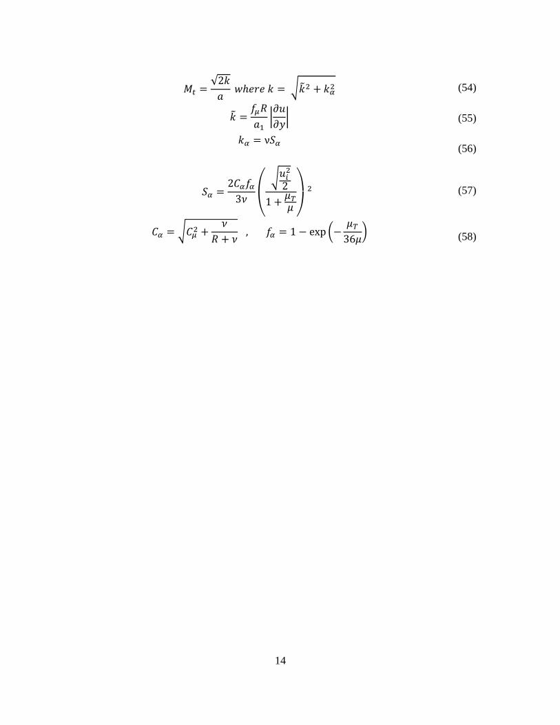
5.3.2 Results with Compressibility Correction for k-ε and SST k-ω Models

Simulations for Seiner nozzle are conducted with standard k-ε model with compressibility

correction, the SST k-ω model with compressibility correction, and the Yang - Shih low

Reynolds number k-ε model with and without compressibility correction. Figure 18 compares the

results obtained from each turbulence model. SST k-ω model with compressibility correction

fails to match the experimental data. The k-ε model with compressibility correction and Yang-

Shih low Reynolds number k-ε model with and without compressibility correction give results in

closer agreement with the experimental data. Results in Fig. 18 show that k-ε model with

compressibility correction performs relatively well in capturing the mixing layer and the length

of the potential core.

Figure 18 Variation in Mach number along the centerline from the jet exit for Seiner nozzle using various standard

turbulence models with Sarkar’s compressibility correction.

29

The importance of capturing the near wall boundary layer profile has been highlighted in

the literature by the results of low Reynolds number k-ε model. Figure 18 shows that the low

Reynolds number k-ε model compressibility correction performs almost as well as the standard

k-ε model with compressibility correction. To evaluate the effect of changing the coefficient of

the dilation dissipation term 𝛼1 in compressibility correction, values of 𝛼1 = 0.5, 0.7, and 1.5

were tested against the reference value of 1.0 in the standard k-ε model. Results are presented in

Fig. 19. As 𝛼1 is increased, the length of the potential core also increases. This is expected since

the effect of compressibility correction increases with increase in the value of 𝛼1. Results in Fig.

19 show that the model with 𝛼1 of 0.5 captures the mixing layer and length of the potential core

better than the model with other values of the coefficient. However, even the best result using the

standard k-ε model with compressibility correction fails to capture the experimental results and

the USM3D results [16].

Figure 19 Variation in Mach number along the centerline from the jet exit for Seiner nozzle using k- ε model with various

values of α1 in Sarkar’s compressibility correction.

30

The results from using the low Reynolds number k-ε models of Yang-Shih, Abid, and

Launder-Sharma with compressibility correction are shown in Fig. 20. This Figure shows that

the compressibility corrected models surprisingly deviate from the experimental data or do not

show any significant improvement. The models with compressibility correction predict either a

longer or same potential core length, and nearly the same mixing layer velocity decay rate. It has

been noted by Gross et al. [17] that Sarkar’s compressibility correction underpredicts the skin

friction by 18 % at Mach 4. From Fig. 13, it can be seen that the SST k-ω baseline model

captures the length of potential core quite accurately compared to the experimental data. The fact

that SST k-ω performs the best in capturing the length of the potential core agrees with the

conventional knowledge that SST k-ω model predicts the wall boundary layer character

accurately for wide range of Mach numbers and geometries. Figure 21 compares the skin friction

data employing the Abid’s low Reynolds number k-ε model with and without compressibility

correction, SST k-ω model, and k-ε model with and without compressibility correction. These

models are chosen for comparison since they capture the length of the potential core quite well.

Figure 21 shows that Abid’s low Reynolds number k-ε model with compressibility correction

overpredicts the skin friction compared to the model without compressibility correction.

However, this phenomena is prevented for the standard k-ε model since it uses a wall function to

calculate the skin friction coefficient. The skin friction coefficient calculated by the k-ε model

matches well with that of SST k-ω model while the skin friction coefficient calculated from

Abid’s low Reynold number k-ε model fails to match that from the SST k-ω model. This results

indicates that the standard k-ε model does not perform well because it requires wall function

while the low Reynolds number k-ε models do not perform well since the compressibility

31

correction makes the models overpredict the skin friction coefficient resulting in longer potential

core.

Figure 20 Variation in Mach number along the centerline from the jet exit for Seiner nozzle using different low Reynolds

number k- ε models with and without Sarkar’s compressibility correction.

32

Figure 21 Comparison of Skin Friction coefficient on the wall of Seiner nozzle using various versions of k- ε models with

and without Sarkar’s compressibility correction; x = 0 is the jet exit.

SST k-ω model with compressibility correction has been previously used to simulate the

jet exhaust from Eggers nozzle which also shows significantly thicker shear layer due to a large

velocity difference between the freestream and the jet exhaust [18]. The model has been shown

to accurately capture the mixing layer and the length of the potential core using the USM3D flow

solver [18]. SST k-ω model without the Sarkar’s compressibility correction and with the

compressibility correction embedded in Fluent was also employed. However, as shown in Figs.

13 and 18, the Fluent simulation using SST k-ω model with and without compressibility

correction fails to agree with the experimental data and USM3D results. The difference between

the flow solver USM3D and ANSYS Fluent is that USM3D code uses a method proposed by

Suzen and Hoffman [15] where the Sarkar’s compressibility correction is only applied in the free

shear layer and is turned-off near the wall. SST k-ω model with compressibility correction

embedded in Fluent also turns the correction on and off depending on the distance to the wall.

33

However, the correction term in Fluent does not include pressure dilation and dilation dissipation

which are included in Sarkar’s correction. Similar effect can be achieved with a wall function

utilized by the standard k-ε model since the method proposed by Suzen and Hoffman [15] also

completely turns-off the compressibility correction in the near wall region. However, there is

inherent difference in the use of wall function vs. the calculation of transport equation down to

the wall. It can be concluded that a blending function applied to the compressibility correction

only in the shear flow region may be needed to correctly capture the mixing layer growth and the

length of the potential core.

5.3.3 Results with Compressibility Correction for Wray-Agarwal Model

The method to obtain the compressibility correction for Wray-Agarwal model was

described in Section 3.3. To compare the effects of two compressibility corrections, that of

Sarkar and Wilcox, they are tested against each other. However, application of different forms of

the compressibility correction is not limited to these two because the type of compressibility

correction can easily be switched as suggested in Eq. (53). Moreover, different coefficients in the

compressibility correction are tested to closely match the experimental results. The major

difference between the compressibility correction of Sarkar and Wilcox is the existence of a

Heaviside function in Wilcox’s formulation that turns off the compressibility term near the wall.

As mentioned in the previous section, compressibility correction can have a negative effect on

the boundary layer profile. In Fig. 22, Mach number profile is plotted against a normalized

distance at the centerline for WA model with either the Wilcox correction or Sarkar correction.

The compressibility coefficient, Ccomp, is plotted with different values of 0.01, 0.05 and 0.3. It is

evident from this figure that compressibility corrected WA model based on either Wilcox or

Sarkar correction gives almost the same results. Also, Ccomp of 0.05 in WA model matches the

34

SST k-ω results with compressibility correction the best. However, like SST k-ω and k-ε models

with compressibility correction, WA model does not perfectly capture the experimental results

along the centerline.

Figure 22 Variation in Mach number along the centerline from the jet exit for Seiner nozzle using Wray-Agarwal model

with Sarkar’s compressibility correction.

5.4 Eggers Nozzle Results Eggers nozzle is another case with shear layer similar to that in case of Seiner nozzle

results. This case provides experimental data in radial direction at various horizontal locations

along the x-axis that allows for a more detailed and better comparison of results from various

turbulence models. Simulations for Eggers nozzle were conducted with SA model, SST k-ω

model with and without compressibility correction, the standard k-ε model with and without

compressibility correction, Launder and Sharma low Reynold number k-ε models with and

35

without compressibility correction and the Wray-Agarwal model with and without

compressibility correction.

5.4.1 Results without Compressibility Correction

Results from baseline turbulence models without compressibility correction in Fig. 23

show the normalized velocity at the centerline of the nozzle obtained from k-ε, Launder-Sharma

Low Reynolds k-ε, Yang-Shih Low Reynolds k-ε, SST k-ω, and Wray –Agarwal turbulence

models without compressibility correction. Results indicate that all models except for SST k- ω

fail to capture the length of potential core. However, k- ε variant models including both the Low

Reynolds k-ε models capture the centerline profile very well downstream. A good performance

of low Reynolds k-ε models is also expected since they performed very well in the case of Seiner

nozzle. Figure 24 shows the radial velocity profile at the exit of the nozzle. The results from Fig.

24 show that the velocity profiles from different models are very similar to each other at the exit

of the nozzle. It confirms the expectation that there will not be much difference in velocity

profiles at the exit.

It is worthy to pay attention to Figures 25, 26 and 27. Figure 25 shows the radial velocity

profile at x/rexit = 26.93. Figure 26 shows the radial velocity profile at x/rexit = 51.96. Figure 27

shows the radial velocity profile at x/rexit=121.3. All figures indicate that, although Wray-

Agarwal turbulence model like other models fails to capture the exhaust plume characteristic

along the centerline, it captures the radial velocity profiles very well. Figures 23 and 25 show

that the results from Wray-Agarwal turbulence model are slightly higher than the experimental

value along the axis. However, away from the centerline, the velocity profiles quickly capture

the experimental results. The next best baseline model that captures the experimental results well

is the Launder-Sharma Low Reynolds k-ε model. Although Launder-Sharma Low Reynolds k- ε

36

model performs better in capturing the experimental radial velocity profile at x/rexit = 51.96 in

Fig. 26, Wray-Agarwal again outperforms in capturing experimental radial velocity profile at

x/rexit =121.3 as shown in Fig. 27. SST k-ω and SA turbulence models without compressibility

correction fail to capture the experimental results.

Figure 23 Variation in u/u_exit along the centerline from the jet exit for Eggers nozzle using various baseline turbulence

models without compressibility correction.

37

Figure 24 Variation in u/u_exit along the radial direction at x/r_exit=3.06 for Eggers nozzle using various baseline

turbulence models without compressibility correction.



38





39

5.4.2 Results with Compressibility Correction SST k-ω, k-ε and Low

Reynolds Number k-ε Models

In this section, the effects of compressibility correction for SST k-ω, k-ε and Low

Reynold number k-ε are examined. All compressibility correction compared in this section use

the Sarkar’s compressibility coefficient of 0.1. As was mentioned in section 5.3.2, there are

multiple variables that affect the results in case of thick shear layer. In particular, the need for

compressibility correction and accurate prediction of boundary layer profile near the nozzle exit

was highlighted. Also, the results for Seiner nozzle indicate that the compressibility correction

has a negative effect on the boundary layer which results in the overall inaccuracy for turbulence

models in prediction of supersonic jet exhaust. Therefore, while compressibility correction is

needed in shear layer to accurately capture the plume characteristics, it should be carefully

turned off to decrease the negative effect it has on the boundary layer near nozzle exit.

Like previous results for Seiner nozzle, low Reynolds number k-ε models with

compressibility correction did not improve the accuracy of the result in predicting the length of

potential core as shown in Fig. 28. Surprisingly the models with compressibility correction

produced more inaccurate results in predicting the length of the potential core. However, the

compressibility correction’s beneficial effect in the prediction of the velocity profile can be

demonstrated when comparing the radial velocity profile results and experimental data. As

mentioned in section 5.4.1, the velocity profiles predicted from different turbulence models are

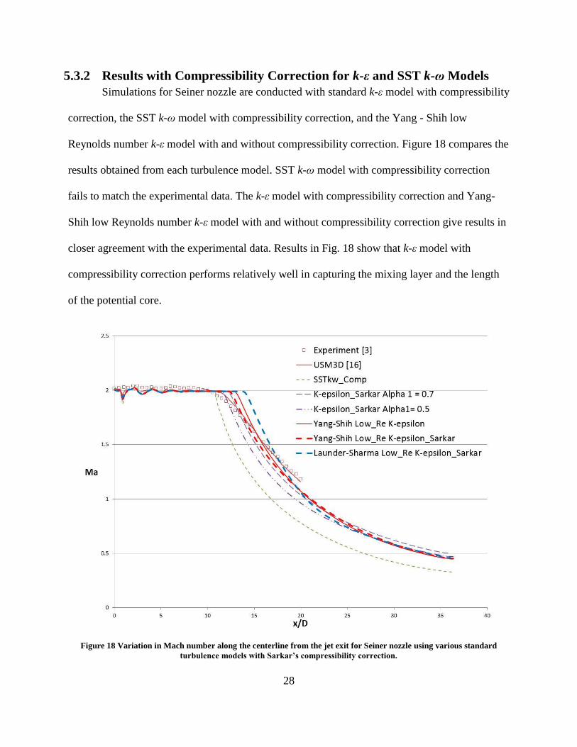
very similar at the exit of the nozzle as shown in Figs 29 and 30. Fig 32 shows how SST k-ω

model with Sarkar’s compressibility correction improves the results remarkably in capturing the

experimental results compared to the baseline model without compressibility correction. Figure

32 shows the radial velocity profile at x/rexit = 26.93. In this figure, while SST k-ω model with

40

compressibility correction goes right through the experimental data profile, SST k-ω without the

compressibility correction slightly underpredicts the data. Figures 34 and 36 show the radial

velocity profile using the SST k-ω model with and without compressibility correction at x/rexit =

51.96 and x/rexit = 121.3, respectively. In these two figures, the difference between the

performance of the compressibility corrected SST k-ω and the its baseline model becomes

greater, showing the beneficial effect of the compressibility correction.

It is worth noting that the compressibility correction may have a negative effect in

predicting the experimental data in some cases if the compressibility correction is not turned-off

in the wall boundary layer near the nozzle exit. Figures 33 and 35 show the radial velocity

profiles obtained using the k-ε and low Reynold number k-ε turbulence model at x/rexit = 51. 96

and x/rexit = 121.3, respectively. The velocity profiles obtained from these two models with

compressibility correction actually deviate from the experimental data. This phenomena may be

due to the fact that the compressibility correction has a negative effect in the prediction of

boundary layer near the jet exit. The fact that these two models do not have the ability to turn-off

the compressibility correction near the wall may cause the inaccuracy in prediction of the radial

velocity profile. This argument is further supported by examining the Wray-Agarwal model

results in Fig. 34 and 36. In these two figures, the Sarkar’s compressibility correction which

applies the correction to all the region including the boundary layer performs considerably worse

than the Wilcox compressibility correction which turns off the correction near the wall via the

Heaviside function.

41

Figure 28 Variation in u/u_exit along the centerline from the jet exit for Eggers nozzle using various turbulence models

with and without Sarkar’s compressibility correction.

Figure 29 Variation in u/u_exit along the radial direction at x/r_exit=3.06 for Eggers nozzle using k-ε, low Reynold

number k-ε turbulence model and SA models with and without Sarkar’s compressibility correction.

42

Figure 30 Variation in u/u_exit along the radial direction at x/r_exit=3.06 for Eggers nozzle using SST k-ω and Wray-

Agarwal turbulence models with and without compressibility correction.



43





44




number k-ε turbulence model and SA models with and without Sarkar compressibility correction.

45



5.4.3 Results with Compressibility Correction for WA Model

In this section, the effects of compressibility correction for Wray-Agarwal turbulence

model with two compressibility corrections are compared along with the SST k-ω model with

compressibility correction. The form of compressibility correction is switched between that by

Sarkar and that by Wilcox. The results from Wray-Agarwal model with and without

compressibility correction suggest correction that Wray-Agarwal turbulence model with Wilcox

compressibility correction performs the best.

Figure 36 shows the normalized velocity profile along the centerline. It shows that none

of the models correctly captures the length of the potential core. However, the best agreement is

obtained either from the Wray Agarwal model without compressibility correction or from Wray-

Agarwal with Wilcox compressibility correction. Figures 38, 39 and 40, which show the radial

46

velocity profiles at x/rexit = 26.93, x/rexit =51.96 and, x/rexit =1212.3, respectively, demonstrate that

the Wray-Agarwal turbulence model with Wilcox compressibility correction formation captures

the experimental results very well. WA model performs better in capturing the radial velocity

profile than the SST k-w model with Sarkar’s compressibility correction as can be seen in Figs.

32, 34, and 36. As mentioned in section 5.4.2, Sarkar’s compressibility correction does not

inhibit the presence of the correction near the nozzle wall which may be the cause of inaccuracy

in the simulation.

An interesting observation from the results in that the Wray-Agarwal model without the

compressibility correction always outperforms the results from the WA model with the

compressibility correction. In Fig 38, it can be seen that the velocity profile from Wray-Agarwal

model starts off slightly higher than the experimental data but quickly captures the experimental

data and performs better than all other models from Fig. 40. It can be seen that the WA model

without the compressibility correction performs as accurately as the model with Wilcox

compressibility correction.

47

Figure 37 Variation in u/u_exit along the centerline from the jet exit for Eggers nozzle using Wray-Agarwal turbulence

models with two different compressibility corrections.

Figure 38 Variation in u/u_exit along the radial direction at x/r_exit=26.93 for Eggers nozzle using Wray-Agarwal

turbulence models with two different compressibility corrections.

48





49

Chapter 6

Conclusions In this thesis, three benchmark axisymmetric supersonic exhaust jet flows have been

computed using ANSYS Fluent with a number of eddy viscosity turbulence models. Four

baseline eddy-viscosity turbulence models (SA, SST k-ω, standard k-ϵ and WA) and their

compressibility corrected forms, and the low Reynold number k-ε models by Yang-Shih, Abid,

Launder-Sharma with Sarkar compressibility correction were employed in the computations. An

auto adapted mesh was used to refine the grid in areas of large density gradients. For the Putnam

nozzle, all baseline turbulence models were able to correctly predict the jet shear layer and the

shock structures in the plume. The inclusion of Sarkar’s compressibility correction in the

turbulence models did not show further improvement in the results. A thicker shear layer exists

in exhaust jet from Seiner nozzle. In this case, the baseline turbulence models were not able to

correctly capture the growth of shear layer and the length of the potential core of the jet. The

inclusion of compressibility corrections improved results somewhat but still satisfactory results

could not be obtained. The good performance of low Reynolds k-ε models indicates that accurate

prediction of boundary layer profile at jet exit is needed in the prediction of shear layer mixing

rate and potential core length. It was shown that the compressibility correction may have a

negative effect on simulation of boundary layer by computing the skin friction on the nozzle wall

using various models. Finally, it was shown for Eggers nozzle that the models that do not have

the ability to turn-off the compressibility correction in boundary layer performed worse than

their baseline models without compressibility correction in several cases. Combined with the

knowledge that the compressibility correction may have a negative effect on the boundary layer

profile accuracy, the computation for two case reconfirmed that capturing boundary layer profile

50

at the nozzle exit is important in capturing the shear layer mixing rate and the length of the

potential core.

Another highlight of the thesis is the performance of the WA model. Although it did not

capture the Mach number profile in Seiner nozzle quite well, it performed very well for Eggers

nozzle. In evaluation of the results with WA model, it was found that the WA model with

Wilcox compressibility correction performed the best in capturing the velocity profile in shear

layer. However, all of the models were not able to capture the length of the potential core even

for the Eggers nozzle.

This study shows the importance of compressibility corrections in the accurate prediction of

compressible mixing layers and jet core length. However, improvements are needed in

turbulence modeling of compressible shear layer flows for accurate predictions of this class of

flow fields.

51

Chapter 7

References [1]“1st AIAA Sonic Boom Prediction Workshop.” http://lbpw.larc.nasa.gov/ [retrieved October 2015]

[2] Putnam, L. E. and Capone, F. J., “Experimental Determination of Equivalent Solid Bodies to Represent

Jets Exhausting into a Mach 2.20 External Stream,” NASA-TN-D-5553, Dec. 1969.

[3] Seiner, J. M., Dash, S. M., and Wolf, D. E., “Analysis of Turbulent Underexpanded Jets, Part II: Shock

Noise Features Using SCIPVIS,” AIAA Journal, Vol. 23, No. 5, May 1985, pp. 669-677.

[4] Eggers, J. M., “Velocity Profiles and Eddy viscosity Distributions Downstream of a Mach 2.22 Nozzle

Exhausting to Quiescent Air,” NASA TN D-3601, September 1966

[5] Chien, K. Y., “Predictions of Channel and Boundary-Layer Flows with a Low-Reynolds-Number

Turbulence Model,” AIAA Journal, Vol. 20, No. 1, 1982, pp. 33-38.

[6] Menter, F. R., “Two-Equation Eddy-Viscosity Turbulence Models for Engineering Applications,”

AIAA J., Vol. 32, No. 8, August 1994, pp. 1598-1605.

[7] Spalart, P. R. and Allmaras, S. R, “A One Equation Turbulence Model for Aerodynamic Flows,” AIAA

Paper 1992-0439, 1992.

[8] Wray, T. J. and Agarwal, R. K., “A New Low Reynolds Number One Equation Turbulence Model Based

on a k-ω Closure,” AIAA Journal, Vol. 58, No. 8, pp. 2216-2227.

[9] Yang, Z. and Shih, T.H., “New Time Scale Based Model for Near-Wall Turbulence,” AIAA Journal,

Vol.31, No.7, 1993, pp.1191-1197.

[10] Launder, B. E. and and Sharma, B. I., “Application of the Energy Dissipation Model of Turbulence to

the Calculation of Flow Near a Spinning Disc,” Letters in Heat and Mass Transfer, Vol. 1, No. 2, 1974, pp.

131-138.

[11] Abid R., “ Evaluation of Two-Equation Turbulence Models for Predicting Transitional flows,” Int. J.

Eng Sci, Vol.31, 1993, pp.831–40.

52

[12] Sarkar, S., Erlebacher, G., Hussaini, M. Y., and Kreiss, H. O., “The Analysis and Modelling of

Dilatational Terms in Compressible Turbulence,” Journal of Fluid Mechanics, 1991. Vol. 227, pp. 473-493.

[13] Wilcox, D. C. “Dilatation-Dissipation Corrections for Advanced Turbulence Models,” AIAA J. Vol.

30, 1992, pp. 2639–2646.

[14] ANSYS® Fluent, Release 15.0, Help System, Theory Guide, ANSYS, Inc.

[15] Suzen, Y. B. and Hoffmann, K. A., “Investigation of Supersonic Jet Exhaust Flow by One- and Two-

Equation Turbulence Models,” AIAA Paper 98-0322, 36th AIAA Aerospace Sciences Meeting, Reno,

Nevada, 1998.

[16] Carter, M. B., Elmiligui, A. A., Campbell, R. L., and Nayani, S. N., “USM3D Prediction of Supersonic

Nozzle Flow,” 32nd AIAA Applied Aerodynamics Conference, 2014.

[17] Gross, N., Blaisdell, G.A., and Lyrintzis, A.S., “Analysis of Modified Compressibility Corrections for

Turbulence Models,” AIAA Paper 2011-279, 2011.

[18] Pandya, M.J., Abdol-Hamid, K.S., and Frink, N. T.: “Enhancement of USM3D Unstructured Flow

Solver for High-Speed High-Temperature Shear Flows.” AIAA 2009-1329, January 2009.

[19] M. M. Rahman, T. Siikonen, and R. K. Agarwal. "Improved Low-Reynolds-Number One-Equation

Turbulence Model," AIAA Journal, Vol. 49, No. 4, 2011, pp. 735-747.

[20] Shoemaker, J. “Performance of Seven Semicircular Lift-Producing Nozzles,” NASA TN D-2731,

1965.

53

Vita Han Ju Lee 701 limit Ave 2S, University City, MO 63130 | 314-570-5707 | hanjulee@@wustl.edu

Education

Washington University in St. Louis Expected to Graduate: Summer 2017

BS/MS Aerospace Engineering 3.80 Overall GPA /3.91 Major GPA

Honors and Awards

2016 Tau Beta Pi Engineering Honor Society

2015 Pi Tau Sigma Mechanical Engineering Honorary

2015 Summer Undergraduate Research Award

2010-2016 6 Dean’s list

Research Experience

Graduate Researcher

Turbulence model research, Advisor: Dr. Agarwal Washington University in St. Louis

Fall 2016- SP2017

• Developed a compressibility correction for Wray Agarwal(WA) turbulence model

• Coded the correction into ANSYS Fluent using C language based user defined function

• Demonstrated the correction for WA model performs better than other compressibility correction forms in the literature by performing both 2D and 3D supersonic jet flow simulations

• Script in preparation for submission at AIAA SciTech 2018

Undergraduate Researcher

Supersonic Nozzle CFD Research, Advisor: Dr. Agarwal Washington University in St. Louis

Fall 2014- SP2016

• Built 2D axi-symmetric hybrid meshes using ANSYS ICEM

• Applied various realistic boundary conditions and simulated supersonic jet cases using ANSYS Fluent

• Studied two supersonic nozzle configurations and analyzed an ability of various turbulence models to capture the compressibility effect at high Mach number in the plume with multiple shock cells using ICEM and ANSYS FLUENT

Publications

• Hanju Lee, Tim Wray, and Ramesh K. Agarwal. "CFD Performance of Turbulence Models for Flow from Supersonic Nozzle Exhausts", 34th AIAA Applied Aerodynamics Conference, AIAA Aviation, (AIAA 2016-3433)

• Lee, Han Ju; Strahan, Nick; and Boyd, Emily, "Turbocharger Jet Engine Build and Engineering Analysis" (2016). Mechanical Engineering and Materials Science Independent Study. Paper 13.

Presentations

• CFD Performance of Turbulence Models for Flow from Supersonic Nozzle Exhausts, Han Ju Lee, Tim Wray and Ramesh K. Agarwal, 34th AIAA Applied Aerodynamics Conference; 2016 June 14, Washington D.C.

54

• CFD Performance of Turbulence Models for Flow from Supersonic Nozzle Exhausts, Han Ju Lee, Tim Wray and Ramesh K. Agarwal, Poster session presented at : Washington University in St. Louis Undergraduate Research Symposium; 2016 Oct 29; St. Louis, MO

CFD Performance of Turbulence Models for Flow from ...

Documents

Transcript of CFD Performance of Turbulence Models for Flow from ...