CFD Modeling of Thermoelectric Air Duct System for Cooling of

Building Envelope.

by

Syaza Yasmin Bt Mohamad Yusoff

16031

Dissertation submitted in partial fulfilment of

the requirements for the

Bachelor of Engineering (Hons) (Mechanical)

JANUARY 2016

Universiti Teknologi PETRONAS

Bandar Seri Iskandar

31750 Tronoh

Perak Darul Ridzuan

i

CERTIFICATION OF APPROVAL

CFD Modeling of Thermoelectric Air Duct System for Cooling of Building

Envelope.

by

Syaza Yasmin Bt Mohamad Yusoff

16031

A project dissertation submitted to the

Mechanical Engineering Programme

Universiti Teknologi PETRONAS

in partial fulfillment of the requirement for the

BACHELOR OF ENGINEERING (Hons)

(MECHANICAL ENGINEERING)

Approved by,

____________________

(Khairul Habib)

UNIVERSITI TEKNOLOGI PETRONAS

TRONOH, PERAK

January 2016

ii

CERTIFICATION OF ORIGINALITY

This is to certify that I am responsible for the work submitted in this project, that the

original work is my own except as specified in the references and acknowledgements,

and that the original work contained herein have not been undertaken or done by

unspecified sources or persons.

_____________________________________

SYAZA YASMIN BT MOHAMAD YUSOFF

iii

ACKNOWLEDGEMENT

In the name of Allah, the Most Gracious, the Most Merciful. Praise to Him the

Almighty that in his will and given strength, the author managed to complete this final

year project within the time required.

Many thanks to the supervisor, Dr. Khairul Habib, for his supervision, support, and

advice not only in project matter but also for the future life and employment. With his

guidance, the project can properly be done without a lot of problem.

The author would like to express gratitude to Kashif Irshad and Salman bin Kashif for

their willingness in teaching all necessary knowledge, procedures and helped to

understand more on the cooling system. These people are so kind and helped a lot in

completing this report. Thanks to all fellow friends and everyone who have directly or

indirectly lent a helping hand here and there. Not forgetting author’s parents and

family, who had always given support in completing this project.

May Allah bless and pay them all.

iv

Contents

CERTIFICATION OF APPROVAL ............................................................................ i

CERTIFICATION OF ORIGINALITY ...................................................................... ii

ACKNOWLEDGEMENT .......................................................................................... iii

List of Figures ............................................................................................................. vi

List of Tables.............................................................................................................. vii

ABSTRACT .............................................................................................................. viii

CHAPTER 1 ................................................................................................................ 1

INTRODUCTION ....................................................................................................... 1

1.1 Background of Study ..................................................................................... 1

1.2 Problem Statement ........................................................................................ 2

1.3 Objective ....................................................................................................... 2

1.4 Scope of Study ............................................................................................... 2

1.5 Relevancy and Feasibility of Study ............................................................... 3

CHAPTER 2 ................................................................................................................ 4

LITERATURE REVIEW............................................................................................. 4

2.1 ThermoElectric Cooler System ..................................................................... 4

2.2 ThermoElectric Configurations ..................................................................... 6

2.3 ThermoElectric Applications ........................................................................ 7

2.4 CFD Simulation Validation and Verification. ............................................... 8

CHAPTER 3 .............................................................................................................. 10

METHODOLOGY ..................................................................................................... 10

3.1 Research Methodology Procedure ............................................................... 10

3.2 Project Activities ......................................................................................... 11

3.3 Tools and Equipment ................................................................................... 13

3.4 Project Key Milestones ............................................................................... 13

3.5 Project Gantt Chart ...................................................................................... 14

v

3.6 Experimental Setup ..................................................................................... 15

3.6.1 Test Room ................................................................................................ 15

3.7 Thermoelectric Air Duct Description .......................................................... 15

3.8 Governing Equation. ................................................................................... 16

3.8.1 Standard k-ε Model .................................................................................. 18

3.9 Simulation Work ......................................................................................... 18

Chapter 4 .................................................................................................................... 21

Result and Discussions ............................................................................................... 21

4.1 Mesh Independence Study ........................................................................... 21

4.2 Effects of the TE-AD system on temperature gradient. .............................. 22

4.3 Effects of the TE-AD system on pressure and air velocity. ........................ 22

4.4 Effects of different air velocity on temperature gradient. ........................... 23

4.5 Comparison of simulation and experimental results. .................................. 25

CONCLUSION AND RECOMMENDATION ......................................................... 26

References .................................................................................................................. 27

APPENDICES ........................................................................................................... 30

vi

List of Figures

Figure 2.1 A Thermoelectric Module [4]. .................................................................... 4

Figure 3.1 Research Methodology Flow Process. ...................................................... 10

Figure 3.2. Project Activities ..................................................................................... 11

Figure 3.3. Simulation Work Flow Chart (ANSYS Fluent)....................................... 12

Figure 3.4. Test room equipped with TE-AD [24] .................................................... 15

Figure 3.5. Breakout Section View of TE-AD ........................................................... 16

Figure 3.6. Temperature Definitions for Thin Wall Model ....................................... 18

Figure 3.7. Named Selections .................................................................................... 19

Figure 4.1. Temperature Data Point ........................................................................... 21

Figure 4.2. Mesh Independence Study. ...................................................................... 22

Figure 4.3. Pressure and Air Velocity Contour for Hot and Cold air duct ................ 23

Figure 4.4. Data Plane in the air duct. ........................................................................ 23

Figure 4.5. Temperature distribution across data plane for various inlet velocity. .... 24

Figure 4.6. Variation of temperature gradient when the TE-AD system operated at 5-

6 A from experimental study [24]. ..................................................................... 25

vii

List of Tables

Table 3.1. Project Gantt Chart.................................................................................... 14

Table 3.2. Range of geometrical and operating parameters for CFD analysis. ......... 16

Table 3.3. Boundary Conditions ................................................................................ 20

Table 4.1. Temperature Contour Calculation ............................................................. 22

Table 4.2. Temperature Gradient for Different Air Velocity ..................................... 24

Table 4.3. Comparison of experimental and simulation data .................................... 25

viii

ABSTRACT

A multi-stage of thermoelectric modules is used in an air duct as a cooling system. The

ThermoElectric Air Duct (TE-AD) system is installed with 24 ThermoElectric

Modules (TEMs) installed with heat sink, cold plate and exhaust fan for air circulation.

To simplify the TE-AD system, a three-dimensional model is proposed and

implemented in a Computational Fluid Dynamics (CFD) simulation environment

(FLUENT). An analysis of results, obtained in the experimental study of the TE-AD

system for cooling of building envelope, shows that temperature gradient of 3.0-5.3°C

between interior and the exterior of the building envelope was achieved. The current

supplied to the TEMs are constant while the air flow rate is varied to investigate the

factor on the performance of the thermoelectric. Using the TE-AD simulation model,

it can be implemented to various CFD models of heat sources to predict the system

performance for optimization.

1

CHAPTER 1

INTRODUCTION

1

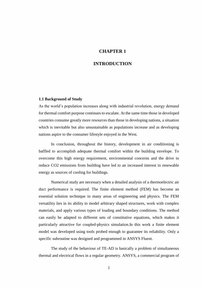
1.1 Background of Study

As the world’s population increases along with industrial revolution, energy demand

for thermal comfort purpose continues to escalate. At the same time those in developed

countries consume greatly more resources than those in developing nations, a situation

which is inevitable but also unsustainable as populations increase and as developing

nations aspire to the consumer lifestyle enjoyed in the West.

In conclusion, throughout the history, development in air conditioning is

baffled to accomplish adequate thermal comfort within the building envelope. To

overcome this high energy requirement, environmental concerns and the drive to

reduce CO2 emissions from building have led to an increased interest in renewable

energy as sources of cooling for buildings.

Numerical study are necessary when a detailed analysis of a thermoelectric air

duct performance is required. The finite element method (FEM) has become an

essential solution technique in many areas of engineering and physics. The FEM

versatility lies in its ability to model arbitrary shaped structures, work with complex

materials, and apply various types of loading and boundary conditions. The method

can easily be adapted to different sets of constitutive equations, which makes it

particularly attractive for coupled-physics simulation.In this work a finite element

model was developed using tools probed enough to guarantee its reliability. Only a

specific subroutine was designed and programmed in ANSYS Fluent.

The study of the behaviour of TE-AD is basically a problem of simultaneous

thermal and electrical flows in a regular geometry. ANSYS, a commercial program of

2

finite element method, solves this type of problems with high accuracy as stated a lot

of validated tests.

. This air-conditioning system, TE-AD (thermoelectric air duct) system use

TEMs (thermoelectric modules) to lower the temperature of the airflow. This study

aims to analyse energy efficiency of the TE-AD system for cooling of building

envelope.

1.2 Problem Statement

Performance of the TE-AD system is directly affected by the ambient temperature and

different flow velocity. In experimental study, the quantitative description of the flow

distribution using measurement is limited to number of points, time, range of problems

and operating conditions. The ANSYS finite element program has a large library of

elements that support structural, thermal, fluid, acoustic, and electromagnetic analyses,

as well as coupled-field elements that simulate the interaction between the above

fields. Examples of ANSYS coupled-physics capabilities include thermal-structural,

fluid-structure, electromagnetic-thermal, thermal-electric, structural-thermal-electric,

piezoelectric, piezoresistive, magneto-structural, and electrostatic-structural analyses

[1]. Using this features, TE-AD model can be adapted into the Ansys Fluent to generate

a general 3-D finite element formulation that can be used to test for various boundary

conditions.

1.3 Objective

In conjunction with above problem statement, the objective is to:

1 To study all temperature dependent characteristics of the TE-AD using

ANSYS CFD-Fluent simulation.

2 To validate the CFD computation result with experimental result.

1.4 Scope of Study

The main scope of this research is to study flow patterns and temperature profile

inside the air duct and to simplify the temperature profile for optimization of the

system performance

3

1.5 Relevancy and Feasibility of Study

The limited number of thermocouple and other measuring device attached to the

system makes it difficult to observe what is happening inside the duct. As a solution

of the problem, using as much as many constraint in geometry modelling available in

the simulation software and taking into considerations all parameter obtained from the

experimental setup to resemble the system and predict flow pattern inside the air duct.

This simulation requires steps to adhere to and proper parameter to be set in

order for the simulation to solve for a converged solution. The project can be

completed in time, given every error can be solve and the value from the experiment

is applicable in the simulation.

4

CHAPTER 2

LITERATURE REVIEW

2

2.1 ThermoElectric Cooler System

In 1821, thermo-electrics effect cause by thermal gradient formed between two

dissimilar conductors was discovered by Thomas Johann Seebeck [2]. This

temperature differences conversion into electricity is the call Seebeck effect.

Semiconductor material inside a Peltier effect device are solid-state energy converters

that can generate heat (or removed) at the junction when electrical current applied to

the material [3].

A TEMs is a circuit containing thermoelectric materials arranged in certain

configurations that either generate electricity from direct heat or convert electricity

into temperature gradient [4]. As illustrated in Figure 2.1, TECs (thermoelectric

coolers) using TEMs to transfer the heat rejected which normally installed with a heat

sink to dissipate the heat to the environment. Cold plate side where the heat is absorbed

cause the enclosure temperature at the side to reduce. For higher temperature gradient

required, the modules can be arranged into multiple columns and rows to achieve the

effect.

Figure 2.1 A Thermoelectric Module [5].

5

In the early 1900’s, metals were still considered to exhibit the best

thermoelectric properties. It had been shown mathematically that a good

thermoelectric material should have a high Seebeck coefficient, high electrical

conductivity, and low thermal conductivity. These characteristics minimize the

thermal effects of Joule heating and dampen the effects of the parasitic heat path which

is opposite the direction of heat pumping. In quantitative terms, it was shown that

practical refrigeration and power generation would be possible with materials, which

hadn’t been invented yet, possessing optimal properties.

With the invention of the transistor, in 1949, came a new type of material called

the semiconductor. It was found that semiconductors could meet the parametric needs

far better than metals, and a new material, bismuth telluride (Bi2Te3) was developed

and found to have advantageous properties near room temperature. Also, because we

typically operate a thermoelectric device thermally in parallel, and electronically in

series, there is a necessity to have materials that transport heat in opposite directions

with respect to current direction. Bi2Te3 is given the ability to be used for the two

inversely related branches by doping it into extrinsic semiconductors.

Due to the state of materials sciences at the time, thermoelectric refrigeration

and power generation efficiencies were significantly worse than their vapor-

compression counterparts. Thermocouples, on the other hand, do not require efficient

thermal to electric energy transformation. For this reason, they have been used and

developed for much longer than Thermoelectric generator and cooler. As materials

sciences advanced, increased efficiencies translated to using ThermoElectric Devices

(TED’s) in commercial and industrial applications requiring small dimensions, gravity

independence, and a solid state/maintenance free design.

In the analysis of TEMs, four different heat effects can be described. These are

Peltier cooling, Peltier heating, Joule heat, and Fourier heat. Joule heat, occurs when

the electrical current is passed through an electrical resistance. It is accepted that half

of this heat is transported from the cold surface and the other part is transported from

the hot surface. Fourier heat, can be defined as the heat transfer from hot surface to

cold surface by conduction.

To achieve a satisfactory thermal comfort there are many limitations to which

TEC is able to operate efficiently. TEC performance are measured with the flexibility

6

of the system to balance the heat transfer by the modules and the ability to optimize

the temperature difference between the enclosure area and the ambient temperature.

The main problem in TEC is to reduce the heat flux across the hot and the cold space

that mostly occurs in the material which separates the flow in the air duct system.

High capital cost and poor power performance of TEC causing current

applications of thermoelectric technology restricted for large enclosure cooling [6].

Other restrictions includes:

Fluctuating environment.

Small scale cooling

Small temperature gradient

Reversible heating and cooling using same modules

Space constraints

Thermoelectric cooling will be considered economically feasible if the coefficient

of performance is about average of vapour compression cooling or higher [7].

Compared to vapour compression cooling which uses rotating equipment in the

compressor, TEC have no moving parts thus results to higher reliability and noise free

operation. TEC cooling can operate using compact and smaller equipment with higher

cooling density. Reversible heating and cooling can be achieved using same modules

by reversing the electrical current flow. Besides, the cooling power can be control

proportional to input power. TEC is flexible in design to meet particular requirements

and refrigerant free system.

2.2 ThermoElectric Configurations

The temperature of the cold side and the cooling capacity of a TEC can be decreased

by multistage TECs. An analytical method was developed for two-stage TECs for

predicting the performance of the module [8]. The performance of a refrigerator with

multistage TECs was investigated by Pan et al. [9]. The performance comparison of

single-stage and multistage TECs was investigated [10]. A three-dimensional model

was developed for the performance optimization of two-stage TECs [11]. Putra et al.

[12] investigated the performance of 5- and 6- stage TECs for cryogenic applications.

7

2.3 ThermoElectric Applications

One of earliest application of TECs are made for cooling small enclosure [13]. In

France, thermoelectric cooling for thermal comfort are used in railroad cabs and

submarines. Under operating condition of 3 ampere, experimental findings of a lab-

scale ceiling, natural convection type TE-AC (thermoelectric air conditioning) with a

natural convection on fin at the cold side and a forced heat convection at the heat sink

at the hot side of the TEMs, the experiment accomplished maximum cooling capacity

of 169 W.

An investigation of thermoelectric air-conditioners compared to vapour

compression and absorption air-conditioner made shows that TE-AC have the highest

purchasing and operating cost under same period of time with highest efficiency at

COP of 0.38-0.45 [14]. A compact TE-AC experiment conducted under operating

condition of 1 A, the cooling capacity of 29 W is achieved. The experiment setup meets

the requirement of 80% acceptability criteria with ANSI/ASHRAE Standard 55

(standard for indoor thermal comfort) with coefficient of performance of 0.34 [15].

Cosnier et al. [16] experimentally studied model of a TEC system using a series

of TEMs. The cold side of the modules is attached with fins forced convected to the

air circulation while the hot sides are in contact with heat sink with fluid as the

medium. Operating under 4 ampere the coefficient of performance of 1.5 to 2 is

achieved, with cooling capacity of 50 W per module. Khire et al [17] proposed TEC

to be implemented for cooling of building envelope for domestic level.

These studies highlight the benefit of the PVMs (photovoltaic modules) to

supply the power to TEC [18]. Kraemer et al. [19] stated that solar cells does not

optimize the lower solar radiation frequency. Several design have been patented using

abundant heat energy from solar radiation to its advantage in thermoelectric

applications. Wahab et al. [20] designed and tested a solar thermoelectric refrigerator.

According to the results, the inside temperature of the refrigerator was decreased from

27°C to 5°C in 44 minutes with a COP of 0.16. Dai [21] also found that the COP value

of a photovoltaic driven TEC was approximately 0.3. Min and Rowe [4] showed that,

for 5°C refrigerator inside temperature and 25°C environment temperature, the COP

value of the thermoelectric refrigerator was between 0.3 and 0.5. Khattab and El

Shenawy [22] investigated to drive TECs by TEGs. It was shown that five TEGs were

able to drive one TEC for Egypt climatic conditions.

8

Yilmazoglu [23] numerical model for prototype thermoelectric heating and

cooling unit is investigated under various TEC voltage differences. Temperature

gradient of 9.1°c and 2.8°c occurred in the hot and cold side air duct.

Different studies made to this day shown that for small scale air-conditioning

system using TEMs technology make it feasible to do small cooling job. A number of

studies suggest application TEMs for small-scale air condition to be powered by

PVMs.

2.4 CFD Simulation Validation and Verification.

Verification and validation provide a framework for rigorously assessing the accuracy

of CFD simulations. Verification deals purely with the mathematics of a chosen set of

equations and can be thought of as solving the equations right. Validation, on the other

hand, entails a comparison to experimental data, that is, real-world observations, and

is concerned with solving the right equations. With regards to the sequence,

verification must be performed first for quantitative validation comparisons to be

meaningful. Error types that are quantified in verification activities include coding

errors, that is, mistakes, incomplete iterative convergence error, round off error, far-

field boundary error, temporal convergence error, and grid convergence (or

discretization) error. This last source of error is related to the adequacy of the

computational mesh employed and is the focus of the current effort.

Carpenter et al. conducted a careful study of the grid convergence behaviour for

a two-dimensional hypersonic blunt-body flow [24]. Their study employed higher-

order methods and omitted any flux limiting at the shock wave. Although the

numerical schemes they employed were formally third and fourth order, they found

that the spatial order of accuracy always reverted to first order on sufficiently refines

meshes. Their findings indicate that even without the use of flux limiters to reduce the

spatial order of accuracy at discontinuities, the information is passed through the shock

wave in a first-order manner (at least in two dimensions and higher). Similar results

have been observed by other authors.

Previous work by Roy et al. and Roy verified the presence of both first- and

second-order errors for a laminar hypersonic blunt body flow when a formally second-

order numerical scheme was used in conjunction with flux limiting at the shock wave.

9

It was shown that the use of a mixed-order numerical scheme resulted in non-

monotonic convergence of certain flow properties as the mesh was refined. This

nonmonotonic grid convergence behaviour was found to occur when the first- and

second-order error terms were of opposite sign, thus leading to error cancellation.

Nonmonotonic grid convergence has been observed by a number of other authors. For

example, Celik and Karatekin examined the flow over a backward-facing step using

the k–ε turbulence model with wall functions [25]. These authors found significant

nonmonotonicity in both the velocity and turbulent kinetic energy profiles as the grid

was refined. The main goal of this work is to explore, in detail, the behaviour of a

mixed first- and second-order numerical scheme as the grid is refined. A secondary

goal is to develop an error estimator that can be applied to such schemes. The test

problem used is the Mach 8 inviscid flow of a calorically perfect gas (° D 1.4) over a

spherically blunted cone. This flow field contains a strong bow shockwave where the

formally second-order spatial discretization reduces to first order.

10

CHAPTER 3

METHODOLOGY

3

The methodology describes the flow of this study process in achieving optimized

solution for the TE-AD system.

3.1 Research Methodology Procedure

Shown in Figure 3.1, is the summary of the process involved in this study.

Figure 3.1 Research Methodology Flow Process.

Identification of Objectives/Problem Statement

Research and Literature Review on Related Topic

Selection of Parameter for the Simulation

Generating 3D Modelling for the Simulation

Run Simulation Solver

Improvements on Model on Encountered Issues

Observation and Analysis of Data

Proposing Optimized Solution

11

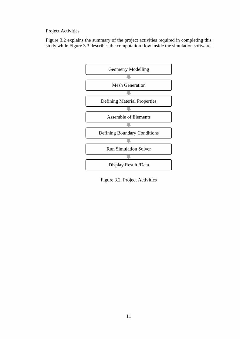
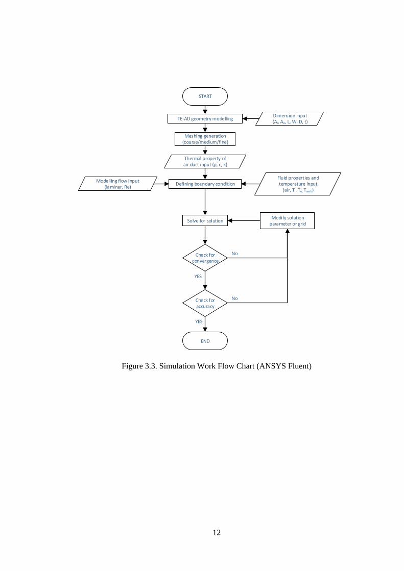
Project Activities

Figure 3.2 explains the summary of the project activities required in completing this

study while Figure 3.3 describes the computation flow inside the simulation software.

Figure 3.2. Project Activities

Geometry Modelling

Mesh Generation

Defining Material Properties

Assemble of Elements

Defining Boundary Conditions

Run Simulation Solver

Display Result /Data

12

START

TE-AD geometry modelling

Thermal property of air duct input (ρ, c, κ)

Dimension input (Ai, Ao, L, W, D, t)

Meshing generation (course/medium/fine)

Defining boundary conditionModelling flow input

(laminar, Re)

Fluid properties and temperature input

(air, Ti, To, Tamb)

Solve for solution

Check for convergence

Modify solution parameter or grid

No

Check for accuracy

No

YES

END

YES

Figure 3.3. Simulation Work Flow Chart (ANSYS Fluent)

13

3.2 Tools and Equipment

ANSYS computational fluid dynamics (CFD) Fluent simulation software and Microsoft

Excel is utilized to predict the impact of fluid flow throughout the TE-AD system.

3.3 Project Key Milestones

• Phase I

- CFD Simulation (Week 11-19)

• Phase II

- Mesh Independence Study (Week 14-20)

14

3.4 Project Gantt Chart

Table 3.1. Project Gantt Chart

Activity

Week

FYP 1 FYP 2

1 2 3 4 5 6 7 8 9 10 11 12 13 14 15 16 17 18 19 20 21 22 23 24 25 26 27 28

Project Title Selection

Preliminary Research

Research on TE-AD

Analysis on common

boundary condition

Software familiarization

CFD Simulation

Mesh Independence Study

Data Analysis

Problem Resolution

Result evaluation and

discussion

15

3.5 Experimental Setup

It was noted that at an applied voltage of 5 V and input current of 6 A, each TEM

module generates 25 W cooling power. Thus, for a cooling load of 589 W, the number

of TEMs required was 24 units which can provide up to 600 W of cooling power at

the given configuration, which was slightly higher than the required cooling load. The

ambient air was circulated inside the test room via the TE-AD system installed on the

north side of the room with the help of a fan as shown in Figure 3.5.

3.5.1 Test Room

Stated by Irshad et. al the experimental process and data collection was conducted at

4°23'11"N 100°58'47"E, Perak, Malaysia under tropical climate. The test room

dimension is 2.8 m wide, 2.7m deep, and 2.5m high as shown in Figure 3.4. The test

room installed with windows (0.304m x 0.22m) with a door (0.821m x 2m).

Figure 3.4. Test room equipped with TE-AD [26]

3.6 Thermoelectric Air Duct Description

The TE-AD is mounted on the wall of the building envelope exterior. The modules

arranged in 8 rows and 3 columns in Figure 3.5. The entire face of the air duct are built

using aluminium sheet with a frame as the foundation. Aluminium foil is wrapped

around the air duct to act as the insulation to reduce the heat flux between the duct

enclosure and the ambient space.

16

Figure 3.5. Breakout Section View of TE-AD

Table 3.2. Range of geometrical and operating parameters for CFD analysis.

Geometrical parameters Range

Entrance length of duct /mm 1070

Width of duct /mm 330

Depth of duct /mm 330

Duct aspect ratio (W/H) 1

3.7 Governing Equation.

The numerical model for fluid flow and heat transfer through an air duct is

developed under the following assumptions:

1. The fluids maintain single-phase, incompressible turbulent flow across the

duct.

2. Steady 2D fluid flow and heat transfer.

3. Both thermally and hydraulically fully developed flow (steady-state

conditions).

4. The thermo-physical properties of both the fluid (air) and the cold plate

(aluminum) are constant (temperature independent).

5. Negligible radiation heat transfer

17

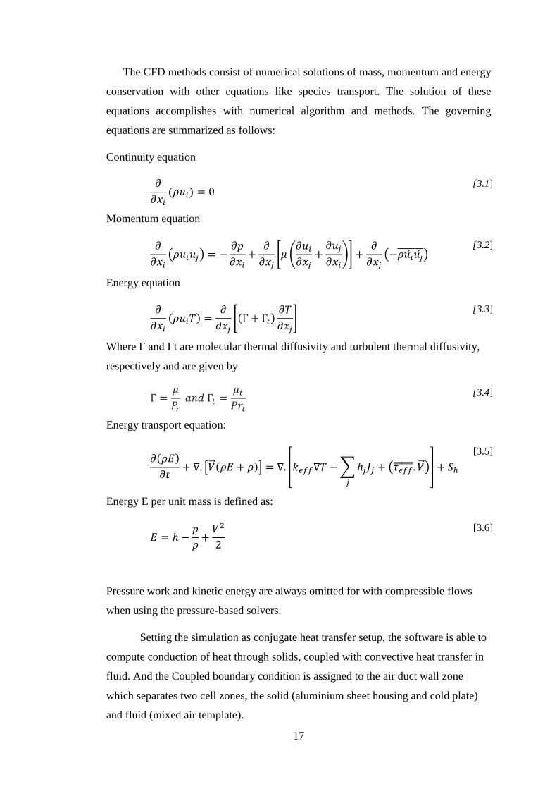
The CFD methods consist of numerical solutions of mass, momentum and energy

conservation with other equations like species transport. The solution of these

equations accomplishes with numerical algorithm and methods. The governing

equations are summarized as follows:

Continuity equation

𝜕

𝜕𝑥𝑖(𝜌𝑢𝑖) = 0

[3.1]

Momentum equation

𝜕

𝜕𝑥𝑖(𝜌𝑢𝑖𝑢𝑗) = −

𝜕𝑝

𝜕𝑥𝑖+

𝜕

𝜕𝑥𝑗[𝜇 (

𝜕𝑢𝑖

𝜕𝑥𝑗+

𝜕𝑢𝑗

𝜕𝑥𝑖)] +

𝜕

𝜕𝑥𝑗(−𝜌𝑢𝑖 𝑢��

) [3.2]

Energy equation

𝜕

𝜕𝑥𝑖

(𝜌𝑢𝑖𝑇) =𝜕

𝜕𝑥𝑗[(Γ + Γ𝑡)

𝜕𝑇

𝜕𝑥𝑗]

[3.3]

Where Γ and Γt are molecular thermal diffusivity and turbulent thermal diffusivity,

respectively and are given by

Γ =𝜇

𝑃𝑟 𝑎𝑛𝑑 Γ𝑡 =

𝜇𝑡

𝑃𝑟𝑡

[3.4]

Energy transport equation:

𝜕(𝜌𝐸)

𝜕𝑡+ ∇. [�� (𝜌𝐸 + 𝜌)] = ∇. [𝑘𝑒𝑓𝑓∇𝑇 − ∑ℎ𝑗𝐽𝑗 + (𝜏𝑒𝑓𝑓 . �� )

𝑗

] + 𝑆ℎ

[3.5]

Energy E per unit mass is defined as:

𝐸 = ℎ −

𝑝

𝜌+

𝑉2

2

[3.6]

Pressure work and kinetic energy are always omitted for with compressible flows

when using the pressure-based solvers.

Setting the simulation as conjugate heat transfer setup, the software is able to

compute conduction of heat through solids, coupled with convective heat transfer in

fluid. And the Coupled boundary condition is assigned to the air duct wall zone

which separates two cell zones, the solid (aluminium sheet housing and cold plate)

and fluid (mixed air template).

18

3.7.1 Standard k-ε Model

Turbulence energy k has its own transport equation:

𝜕(𝜌𝑘)

𝜕𝑡+

𝜕(𝜌��𝑖𝑘)

𝜕𝑥𝑖= −𝜌��𝑖��𝑗

𝜕��𝑖

𝜕𝑥𝑗− 𝜌𝜀 +

𝜕

𝜕𝑥𝑗[(𝜇 +

𝜇𝑡

𝜎𝑘)

𝜕𝑘

𝜕𝑥𝑗]

[3.7]

This requires a dissipation rate, ε, which is entirely modeled phenomenologically

(not derived) as follows:

𝜕(𝜌𝜀)

𝜕𝑡+

𝜕(𝜌��𝑖𝜀)

𝜕𝑥𝑖=

𝜕

𝜕𝑥𝑗[(𝜇 +

𝜇𝑡

𝜎𝜀)

𝜕𝜀

𝜕𝑥𝑗] + ∁1𝜀𝑃𝑘

𝜀

𝑘− ∁2𝜀𝜌

𝜀2

𝑘

[3.8]

Dimensionally, the dissipation rate is related to k and a turbulence length scale:

𝜀~

𝑘3/2

𝐿𝑡

[3.9]

Together with the k equation, eddy viscosity can be expressed as:

𝜇𝑡 = 𝜌∁𝜇𝐿𝑡√𝑘 = 𝜌∁𝜇

𝑘2

𝜀

[3.10]

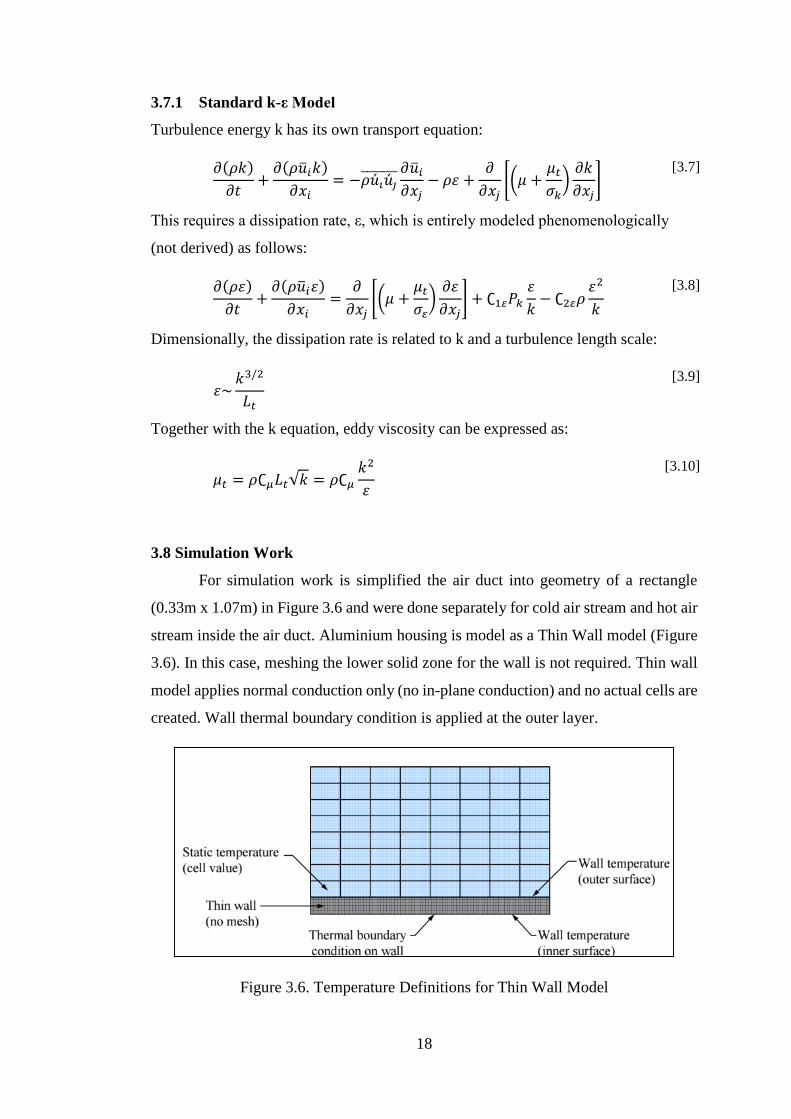
3.8 Simulation Work

For simulation work is simplified the air duct into geometry of a rectangle

(0.33m x 1.07m) in Figure 3.6 and were done separately for cold air stream and hot air

stream inside the air duct. Aluminium housing is model as a Thin Wall model (Figure

3.6). In this case, meshing the lower solid zone for the wall is not required. Thin wall

model applies normal conduction only (no in-plane conduction) and no actual cells are

created. Wall thermal boundary condition is applied at the outer layer.

Figure 3.6. Temperature Definitions for Thin Wall Model

19

Natural convection occurs when heat is added to fluid and fluid density varies with

temperature. Flow is induced by force of gravity acting on density variation. When

gravity term is included, pressure gradient and body force term in the momentum

equation are re-written as:

−

𝜕𝑝

𝜕𝑥+ 𝜌𝑔 →

𝜕��

𝜕𝑥+ (𝜌 − 𝜌0)𝑔

[3.11]

Where,

�� = 𝑝 − 𝜌0𝑔𝑥 [3.12]

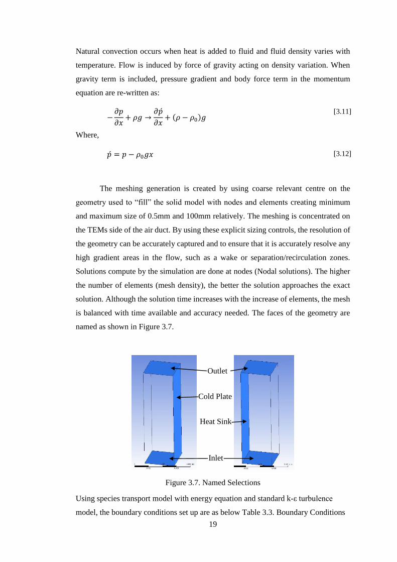
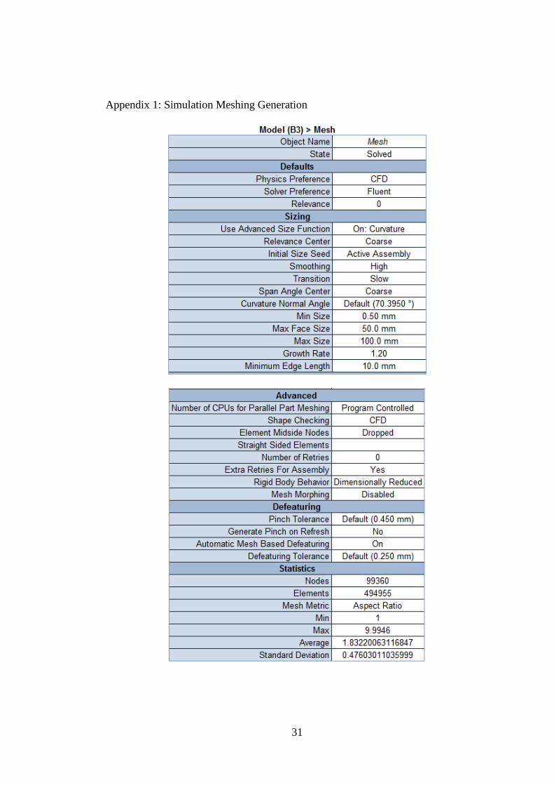
The meshing generation is created by using coarse relevant centre on the

geometry used to “fill” the solid model with nodes and elements creating minimum

and maximum size of 0.5mm and 100mm relatively. The meshing is concentrated on

the TEMs side of the air duct. By using these explicit sizing controls, the resolution of

the geometry can be accurately captured and to ensure that it is accurately resolve any

high gradient areas in the flow, such as a wake or separation/recirculation zones.

Solutions compute by the simulation are done at nodes (Nodal solutions). The higher

the number of elements (mesh density), the better the solution approaches the exact

solution. Although the solution time increases with the increase of elements, the mesh

is balanced with time available and accuracy needed. The faces of the geometry are

named as shown in Figure 3.7.

Figure 3.7. Named Selections

Using species transport model with energy equation and standard k-ε turbulence

model, the boundary conditions set up are as below Table 3.3. Boundary Conditions

Outlet

Inlet

Cold Plate

Heat Sink

20

Table 3.3. Boundary Conditions

Operating Parameter Range

Cold plate temperature 283.15 k

Heat sink temperature 400k

Inlet velocity Magnitude 0.5 m/s

Outlet gauge pressure 1 atm

Insulated wall heat flux 0 w/ m2

Insulation Sheet External emissivity 0.03

Before the simulation is started, grid check is performed to avoid problems due

to incorrect mesh connectivity and maximum cell skewness are observed to be below

1. All physical dimensions are initially assumed to be in meters. The model grid are

scaled accordingly. Energy underrelaxation factor are set between 0.95 and 1, because

for problems with conjugate heat transfer, when the conductivity ratio is very high,

smaller values of the energy underrelaxation factor practically stall the convergence

rate. For problems with conjugate heat transfer, when the conductivity ratio is very

high, smaller values of the energy underrelaxation factor practically stall the

convergence rate.

Node-based gradients with unstructured tetrahedral meshes is used. The node-

based averaging scheme is known to be more accurate than the default cell-based

scheme for unstructured meshes, most notably for triangular and tetrahedral meshes

[1]. While monitoring convergence with residuals history, residual plots can show

when the residual values have reached the specified tolerance. After the simulation,

residuals have decreased by at least 3 orders of magnitude to at least 10-3. For the

segregated solver, the scaled energy residual must decrease to 10-6. Also, the scaled

species residual may need to decrease to 10-5 to achieve species balance.

To conclude, the simulation was solved under steady state conditions with

pressure-based solver and operating conditions of negative gravitational acceleration

in y-axis direction. Energy equation, standard k-ε turbulence and species transport

model were used. Both simulation, the solution converged under 300 number of

iterations performed by SIMPLE algorithm.

21

Chapter 4

Result and Discussions

4 Result and Discussions

4.1 Mesh Independence Study

Grid convergence is the term used to describe the improvement of results by

using successively smaller cell sizes for the calculations. A calculation should

approach the correct answer as the mesh becomes finer, hence the term grid

convergence. The normal CFD technique is to start with a coarse mesh and gradually

refine it until the changes observed in the results are smaller than a pre-defined

acceptable error.

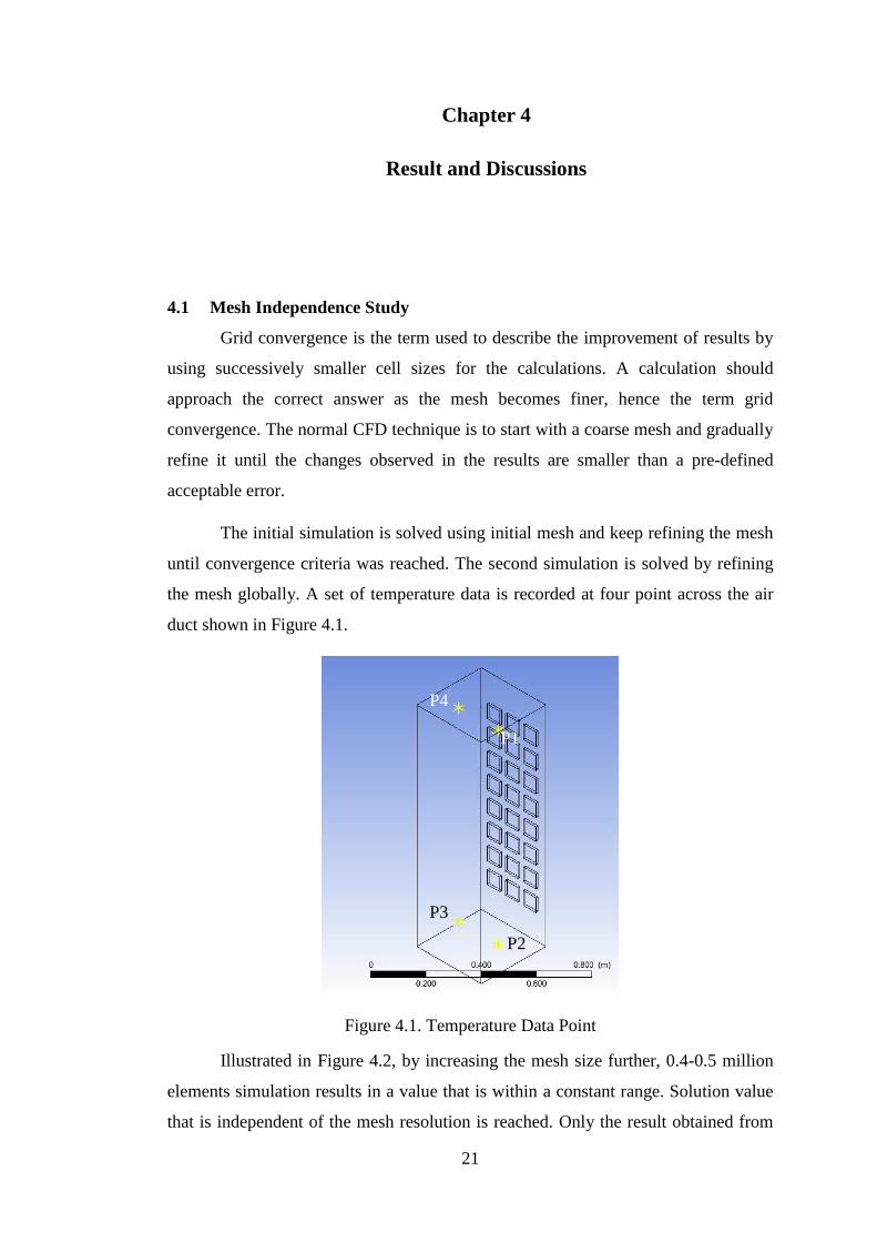
The initial simulation is solved using initial mesh and keep refining the mesh

until convergence criteria was reached. The second simulation is solved by refining

the mesh globally. A set of temperature data is recorded at four point across the air

duct shown in Figure 4.1.

Figure 4.1. Temperature Data Point

Illustrated in Figure 4.2, by increasing the mesh size further, 0.4-0.5 million

elements simulation results in a value that is within a constant range. Solution value

that is independent of the mesh resolution is reached. Only the result obtained from

P1

P4

P3

P2

22

the simulation meshing generation with no of elements above 400k is acceptable. This

step is applied for every simulation computed in the ANSYS Fluent.

Figure 4.2. Mesh Independence Study.

4.2 Effects of the TE-AD system on temperature gradient.

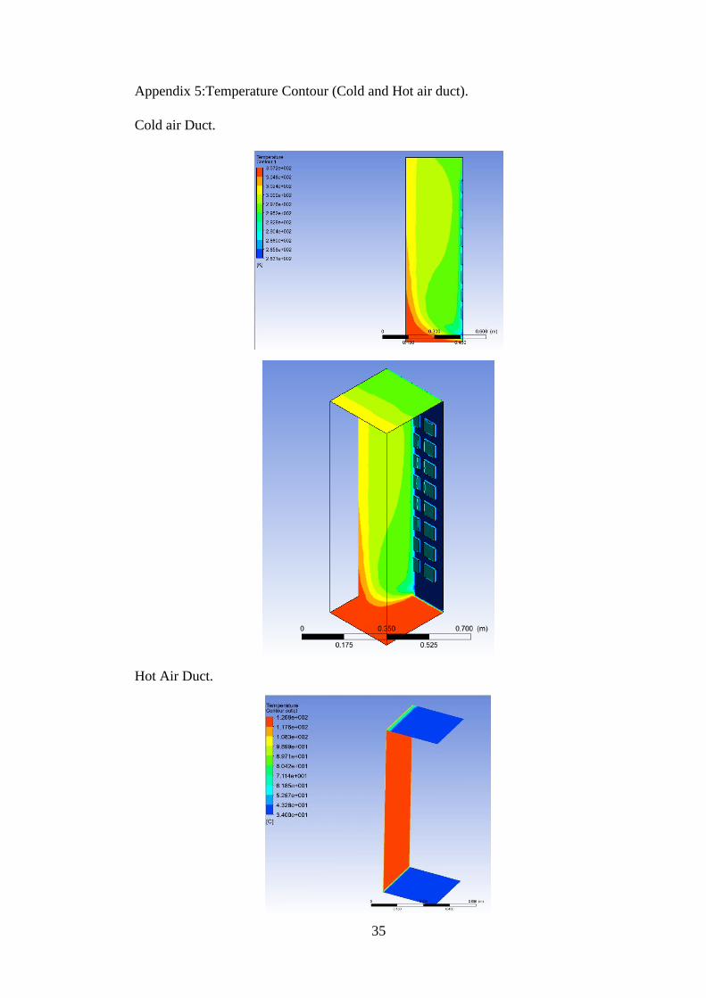
The summary of the temperature profile calculation are as shown in Table 4.1.

Temperature Contour Calculation. Refer to Appendix 5 for the temperature contour

inside the air duct.

Table 4.1. Temperature Contour Calculation

Air Duct Cold Hot

Temperature (min), K 283.2 307.2

Temperature (max), K 307.2 400

Average Temperature (Inlet), K 307.2 307.2

Average Temperature (Outlet), K 303.4 310.1

Temperature gradient between Inlet and

Outlet, K

3.8 2.9

4.3 Effects of the TE-AD system on pressure and air velocity.

The specified boundary conditions for air velocity and outlet pressure cause

the solutions to solve the simulation under constant pressure and velocity in Figure

4.3.

294

296

298

300

302

304

306

308

0 100000 200000 300000 400000 500000 600000Tem

per

atu

re,

deg

ree

celc

ius

No of elements

Mesh Independence Study

P1(edge) P2(edge) P3(middle) P4(middle)

23

Figure 4.3. Pressure and Air Velocity Contour for Hot and Cold air duct

4.4 Effects of different air velocity on temperature gradient.

Using plane distributed along the air duct, the average temperature on each

plane is taken in Figure 4.4.

Figure 4.4. Data Plane in the air duct.

24

Figure 4.5. Temperature distribution across data plane for various inlet velocity.

The effect of air velocity on temperature gradient measured in cold air duct

was investigated. In Table 4.2, for different air velocity the temperature gradient vary

between 8.913 and 2.297 degrees.

Table 4.2. Temperature Gradient for Different Air Velocity

Inlet Velocity,m/s 0.05 0.1 0.2 0.3 0.4 0.5

Temperature

Gradient, degree 8.913 7.969 6.596 4.981 3.78 2.297

296

298

300

302

304

306

308

0 2 4 6 8 10 12 14

Tem

per

atu

re,

K

Plane0.05 m/s 0.1 m/s 0.2 m/s 0.4 m/s 0.5 m/s

25

4.5 Comparison of simulation and experimental results.

Figure 4.6. Variation of temperature gradient when the TE-AD system operated at 5-

6 A from experimental study [26].

To calculate the mean of distribution,

𝜇 = ∑[𝑥. 𝑃(𝑥)] [4.1]

The simulated and the experimental results of the TE-AD system were

compared and found in good agreement. Since the optimum performance of the TE-

AD system was found in the current range of 5-6 A under inlet velocity of 0.4 m/s, so

experimental results of indoor temperature for this range were compared with

simulated results and presented in Table 4.3. Results show that the temperature

difference between experimental and simulation data was less than ±0.4 °C.

Table 4.3. Comparison of experimental and simulation data

Experimental Simulation

Temp. gradient,

°C 4.2 3.8

Percentage

error, % 9.5

0

2

4

6

8

10

12

14

0 1 2 3 4 5 6

freq

uen

cy

Temperature Gradient, degree

Temperature Gradient Frequency

26

CHAPTER 4

CONCLUSION AND RECOMMENDATION

The purpose of the simulations is to replicate the same setup as the

experimental and to observe the behaviour of the performance under different

conditions. The TE-AD simulation model provide detailed temperature profiles in the

air duct and velocity contours as well as the temperature drop in the air duct. In

comparison to the benchmark experimental analyses, the results validate the accuracy

of the simulation model. According to the simulation study, it was possible to cool

down air flows by 4°C for the assigned boundary conditions. The study shows that it

is possible to use TECs as an alternative method for HVAC applications with properly

designed air duct system.

Nonetheless, the verification and validation procedures and methodology are

recommended for use. Use of such procedures and methodology should be helpful in

guiding future developments in CFD through documentation, verification, and

validation studies and in transition of CFD codes to design through establishment of

credibility. Presumably, with a sufficient number of documented, verified, and

validated solutions along with selected verification studies a CFD code can be

accredited for a certain range of applications. The contribution of the present work is

in providing procedures and methodology for the former, which hopefully will help

lead to the better future simulation. Although validation is made for assessing the

model uncertainty by using the experimental data under same operating conditions,

much more work can be integrated into the simulation for additional error source and

alternative error by using user defined function for the temperature input and material

selection to account for fluctuating environment and different materials of the air duct

for the system optimization.

As suggested by many previous study, integrating this TE-AD system with

photovoltaic modules provide utilization of solar energy, especially in cooling

applications in tropical climate.

27

References

[1] "ANSYS Release 9.0 Documentation," 2004. [Online].

[2] W. R. Fahrner and S. Schwertheim, "Semiconductor thermoelectric

generators," Stafa-Zuerich, Trans Tech, 2009.

[3] G. S. Nolas and J. Sharp, "Historical Development," Thermoelectrics: basic

principles and new materials developments, pp. 1-33, 2001.

[4] D. M. Rowe, "Thermoelectric Module Design Theories," in Thermoelectrics

handbook macro to nano, Boca Raton, CRC/Taylor & Francis, 2006, pp. 1-16.

[5] "Frequently Asked Questions About Our Cooling And Heating Technology,"

[Online]. Available: http://tellurex.com/wp-content/uploads/2014/04/peltier-

faq.pdf. [Accessed October 2015].

[6] D. R. Brown, J. A. Dirks, N. Fernandez and T. E. Stout, "The Prospects of

Alternatives to Vapor Compression Technology for Space Cooling and Food

Refrigeration Applications," 2010.

[7] L. G. Stokholm, "Reliability of thermoelectric cooling systems," in

Proceedings of Xth International Conference on Thermoelectrics, Cardiff,

1991.

[8] M. Ma and J. Yu, "An analysis on a two-stage cascade thermoelectric cooler

for electronics cooling applications," International Journal of Refrigeration,

no. http://dx.doi.org/10.1016/j.ijrefrig, 2013.

[9] Y. Pan, B. Lin and J. Chen , "Performance analysis and parametric optimal

design of an irreversible multi-couple thermoelectric refrigerator under various

operating conditions," vol. 84, pp. 882-892, 2007.

[10] G. Karimi, J. Culham and V. Kazerouni, "Performance analysis of multi-stage

thermoelectric coolers," International Journal of Refrigeration, vol. 34, pp.

2129-2135, 2011.

28

[11] X. Wang, Q. Wang and J. Xu, "Performance analysis of two-stage TECs

(thermoelectric coolers) using a three dimensional heat-electricity coupled

model," Energy, no. energy.2013.10.047, 2013.

[12] N. Putra, A. Sukyono, D. Johansen and F. Iskandar, "The characterization of a

cascade thermoelectric cooler in a cryosurgery device, Cryogenics," vol. 50,

pp. 759-764, 2010.

[13] J. Stockolm, L. Pujol-Soulet and P. Sternat, "Prototype thermoelectric air

conditioning of a passenger railway coach," in 4th Intern Conf on

Thermoelectric Energy Conversion, Arlington, 1982.

[14] S. Riffat and G. Qiu, "Comparative investigation of thermoelectric air-

conditioners versus vapour compression and absorption air-conditioners,"

Applied Thermal Engineering, vol. 24, p. 1979–1993, 2004.

[15] S. Maneewan, W. Tipsaenprom and C. Lertsatitthanakorn, "Thermal Comfort

Study of a Compact Thermoelectric Air Conditioner," Journal of Electronic

Materials, vol. 39, p. 1659–1664, 2010.

[16] M. Cosnier, G. Fraisse and L. L, "An experimental and numerical study of a

thermoelectric air-cooling and air-heating system," International Journal of

Refrigeration, vol. 31, pp. 1051-1062, 2008.

[17] R. Khire, A. Messac and S. VanDessel, "Design of thermoelectric heat pump

unit for active building envelope," International Journal of Heat and Mass

Transfer, vol. 48, p. 4028–4040, 2005.

[18] S. Van, "Feasibility of photovoltaic-Thermoelectric hybrid modules," Applied

Energy, vol. 88, pp. 2785-2790, 2011.

[19] D. Kraemer, L. Hu, A. Muto, X. Chen, G. Chen and M. Chiesa, "Photovoltaic-

thermoelectric hybrid systems:A general optimization methodology," Appl.

Phys. Lett. Applied Physics Letters, p. 243503, 2008.

[20] S. Abdul Wahab, A. Elkamel , A. Al-Damkhi, I. Al-Habsi, H. Al-Rbai'ey, A.

Al-Battashi, A. Al-Tamimi, K. Al-Mamari and M. Chutani, "Design and

29

experimental investigation of portable solar thermoelectric refrigerator,"

Renewable Energy, vol. 34, pp. 30-34, 2009.

[21] Y. Dai, R. Wang and L. Ni, "Experimental investigation and analysis on a

thermoelectric refrigerator driven by solar cells," Solar Energy Materials &

Solar Cells, vol. 77, pp. 377-391, 2003.

[22] N. Khattab and E. El Shenawi, "Optimal operation of thermoelectric cooler

driven by solar thermoelectric generator," Energy Conversion and

Management, vol. 47, pp. 407-426, 2006.

[23] M. Yilmazoglu, "Experimental and numerical investigation of a prototype

thermoelectric heating and cooling unit," Energy and Buildings (2015), no.

http://dx.doi.org/10.1016/j.enbuild.2015.12.046.

[24] M. Capenter and J. Casper, "Accuracy of Shock Capturing in Two Spatial

Dimensions," AIAA Journal, vol. 37, no. 9, pp. 1072-1079, 1999.

[25] I. Celik and O. Karatekin, "Numerical Experiments on Application of

Richardson Extrapolation with Nonuniform Grids," Journal of Fluids

Engineering, vol. 119, no. 3, pp. 584-590, 1997.

[26] K. Irshad, K. Habib, N. Thirumalaiswamy and B. B. Saha, "Performance

analysis of a thermoelectric air duct system for energy-efficient buildings,"

Energy, pp. 1009-1017, 2015.

[27] M. A. Ghazali and R. A. M. Abdul, "The Performance of Three Different Solar

Panels for Solar Electricity Applying Solar Tracking Device under the

Malaysian Climate Condition," Energy and Environment Research, 2012.

30

APPENDICES

Appendix 1: Simulation Meshing Generation

Appendix 2: Simulation Mesh

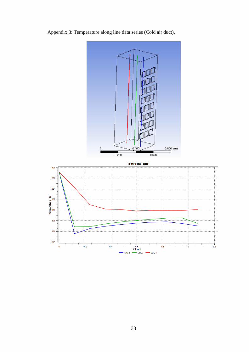
Appendix 3: Temperature along line data series.

Appendix 4: Pressure along line data series (Cold air duct).

Appendix 5:Temperature Contour (Cold air duct).

31

Appendix 1: Simulation Meshing Generation

32

Appendix 2: Simulation Mesh

33

Appendix 3: Temperature along line data series (Cold air duct).

34

Appendix 4: Pressure along line data series (Cold air duct).

35

Appendix 5:Temperature Contour (Cold and Hot air duct).

Cold air Duct.

Hot Air Duct.