* Corresponding author.

1944-3994/1944-3986 © 2020 Desalination Publications. All rights reserved.

Desalination and Water Treatment www.deswater.com

doi: 10.5004/dwt.2020.26211

201 (2020) 95–109October

CFD for the optimization of ventilation mode of an aeration tank

W. Wei*, Ch. Lou, J. Wei, X. Zhao, Y. ChangState Key Laboratory of Eco-hydraulics in Northwest Arid Region of China, Xi’an University of Technology, Xi’an, Shaanxi 710048, China, Tel. +86 15596886263; email: wwl_p@126.com (W. Wei), Tel. +86 18292878016; email: 1398469272@qq.com (Ch. Lou), Tel. +86 18629352022; email: Jwei1995@126.com (J. Wei), Tel. +86 15191913820; email: XZhao@126.com (X. Zhao), Tel. +8613991987708; email: 564391746@qq.com (Y. Chang)

Received 18 September 2019; Accepted 7 June 2020

a b s t r a c tThis paper is concerned with a numerical simulation of gas–liquid two-phase flow in an aeration tank using an Euler–Euler multiphase flow model with the renormalized group (RNG) k–ε turbu-lent model (in FLUENT6.3.26), by which the variations of air volume fraction (AVF) and turbulence kinetic energy (TKE) along water depth and the distributions of velocities of gas and liquid phases were obtained. By analyzing the change of physical parameters of the aeration tank under various operating conditions, the optimal spacing of 0.13 m between the aeration pipes was obtained, and also the relationship between the change of AVF and ventilation velocity in the aeration tank was obtained so as to define a better range of ventilation velocity of 6.25–8.25 m/s. The research results show that the optimal design parameters can be determined by comparing the hydraulic characteris-tics simulated by the mathematical model, and have a more direct guiding significance for the design of practical aeration tanks.

Keywords: Numerical simulation; Flow field; Air volume fraction; Euler–Euler multiphase flow model; Aeration tank

1. Introduction

Aeration tank is an important part of activated sludgetreatment system, and its cost accounts for a large proportion of the total cost of sewage treatment system. The efficiency of sewage treatment system largely depends on the optimi-zation of structure and operation mode of an aeration tank. It is of great theoretical significance and engineering value to analyze the various factors affecting the aeration efficiency of an aeration tank based on the properties of gas–liquid two-phase flow fields. In recent years, many scholars have studied the behavior of gas–liquid two-phase flow in an aeration tank, and further focus on the residence time, size distribution of bubbles, regularity of bubble breakup and polymerization, and the improvement of related mathemat-ical models [1–3]. With the development of computational

fluid dynamics (CFD) along with biological dynamics mod-els, we have well simulated the gas–liquid flows and the biochemical process in aeration tanks. By adding tracer par-ticles into an aeration tank model, and then monitoring the movement of the tracer particles, we can accurately obtain the residence time of oxygen in the aeration tank [4,5]. In a real biological reaction process of an aeration tank, besides the traditional ammonia nitrogen, the change of tempera-ture is also a very intuitive tracking parameter for reflecting the flow fields [6]. In terms of the biological reaction in an aeration tank, the efficiency of oxygen mass transfer is the most important factor to be studied. The bio-kinetic model can be used to simulate the transfer law between oxygen and floc, and sewage, which can truly reflect the interaction process between sewage and oxygen in the aeration tank [7]. In CFD, gas–liquid two-phase flow in aeration tank is often

W. Wei et al. / Desalination and Water Treatment 201 (2020) 95–10996

simplified to be a bubble plume; Yang [8] used a two-phase flow model to simulate a bubble plume, and analyzed the simulation results in detail by combining with the related experiments. As far as simulation is concerned, different turbulence models and different meshing methods also have a great difference in capturing bubble plume flows [9]. In the prediction of bubble diameter distribution and void fraction, the drag coefficient between gas and liquid phases has a great impact on the fine simulation of bubble plume, and Cheng [10] used a better drag coefficient model to obtain a more precise result. With the development of experimen-tal technology, the measurement of bubble plume is becom-ing more and more accurate; the whole flow pattern and its development, and turbulent diffusion near the plume can be accurately measured [11]. The process of formation and development of bubbles in a plume generator [12], and the breakup, aggregation, and diameter distribution of bubbles in the rising process can also be captured [13]. Different multi-phase models were used to simulate the physical plume model, and the results were compared with plume experiments, which provide a basis for optimization of the multi-phase model by considering the influence of various factors [14,15]. From the aspect of improving the mathemat-ical model, some researchers mainly focus on the turbulence models and multiphase flow models, and then compare the difference [16,17] between the different turbulence models, and the multiphase flow models. In addition, in order to truly reflect the law of bubble coalescence and collapse in water, some scholars added a mathematical model reflect-ing bubble coalescence in the multi-phase flow model, which better simulated the real motion state [18]. Shean et al. [19] proposed a model tested by experiments, which pro-vides a method to improve the operating stability of aerated tanks through better modeling of the dynamic pulp height changes that result from changes in air flow rate. Terashima et al. [20] conducted CFD calculations to simulate the hydraulics in different aeration tanks, and the calculated values of the volumetric oxygen mass transfer coefficient were compared with experimentally measured data. The results of the calculations indicate that the coarse-bubble diffusers, fine-pore diffusers, and slitted membrane diffus-ers have bubble sizes of 7–8, 5–6 mm, and approximately 3 mm, respectively. Herrmann-Heber et al. [21] performed a numerical simulation in investigating the mass transfer of pulsed aeration modes in comparison to constant flow aer-ation in a test geometry, by which the effects of flow rate, pulsation frequency, and bubble size and injection depth on mass transfer were studied. The oxygen transfer efficien-cies derived from the simulations are in good agreement with the experimental results from Alkhalidi et al. [22].

In this paper, from the view point of the air–liquid flow field in an aeration tank, various factors affecting the behavior of aeration were studied by solving the Euler–Euler multiphase flow model with the RNG k–ε turbulent model. The aeration process of the aeration tank was simplified as a gas–liquid plume, which can reduce a lot of simulation work. According to the simulation results under the same discharge of aeration mass per unite time, we determined the better spacing between aeration pipes and the better size and density of ventilation holes in the aeration pipes of the aeration tank, and also obtained the relationship between

the changes of AVF and ventilation velocity in the aeration tank so as to define a better range of ventilation velocity. The results of the study will have a more direct guiding significance for practical aeration tanks.

2. Mathematical model

In the Euler–Euler method, all phases are taken as a continuous medium, and they penetrate and dissolve each other. Since the volume occupied by one phase can no lon-ger be occupied by other phases, the concept of volume fraction has been introduced, which represents the ratio of the space occupied by one phase to the space of the total multiphase in a mesh. The volume fraction is a continuous function of time and space, and the sum of volume frac-tions of all the phases equals to 1, that is, Σn

q = 1αq = 1, where αq is the volume fraction of q phase; q represents a phase, and n denotes the total number of the phases.

A set of equations can be derived from the conservation equations of mass and momentum for all phases, which is called a multiphase flow model. In FLUENT software, there are three kinds of multiphase flow models: volume of fluid (VOF) model, mixture model, and Euler–Euler multiphase model. The conservation equations of the Euler–Euler mul-tiphase model are the continuity and momentum equations, described as follows [23–25]:

Continuity equation:

∂∂( ) + ∇ ⋅ ( ) =

=∑t

v mq q q q q pqq

n

α ρ α ρ� �

1 (1)

where vq is the velocity of q phase; ρq is the physical density of q phase; mpq is the mass transfer from p phase to q phase. Therefore, from the conservation of mass, the following equations can be obtained:

m mpq qp= − (2)

mpp = 0 (3)

Momentum equation:

∂∂( ) + ∇ ⋅ ( ) = − ∇ +∇ ⋅ + +( ) +

=tv v v P R m vq q q q q q q q pq pq pq

p

n

α ρ α ρ α τ� � � �

� �1∑∑

+ +( )α ρq q q q vm qF F F� � �

lift , , (4)

where τ is the pressure strain tensor of q phase, expressed as:

τ α µ α λ µ= ∇ +( ) + −

∇ ⋅q q q q

Tq q q qv v v I 2

3 (5)

where μq and λq are the shear force and volume viscosity of q phase, respectively;

Fq is the external volume force of q phase;

F qlift , is the lift force of q phase;

Fvm q, the virtual mass force of q phase;

Rpq is the interaction force between p and q phases, and P is the pressure of q phase; vpq the relative

97W. Wei et al. / Desalination and Water Treatment 201 (2020) 95–109

velocity between p and q phases, defined as follows: if mpq > 0 (the mass transfer of p phase to q phase), v vpq q= ; if mpq < 0 (the mass transfer of q to p phase), v vpq q= , and v vpq qp= .

In Eq. (4), the interaction force,

Rpq, can be expressed as:

R K v vpqp

n

pq p qp

n

= =∑ ∑= −( )

1 1 (6)

where Kpq(=Kqp) stands for the momentum exchange coeffi-cient between p and q phases.

And the lift force,

Flift, acting on the second phase par-ticles (droplets and bubbles), is mainly due to the velocity gradient of main phase flow field, and can be written as:

F v v vq p p q qlift = − − × ∇×( )0 5. ρ α (7)

In general, the lift force is not important relative to drag force; therefore, in most cases, it is ignored.

In multiphase flow, when the second phase accelerates relative to the main phase, the effect of virtual mass force appears. When the inertia of the main phase mass encounters the accelerated particle, the virtual mass force,

Fvm, in Eq. (4), is applied to the particle, and is expressed as:

Fdqvdt

dpvdtvm p q

q p= −

0 5. α ρ (8)

with the expression of dq/dt as:

dqdt t

vpφ φ

φ( )

=∂( )∂

+ ⋅∇( ) (9)

For liquid–liquid flows, the second phase is assumed to appear in the form of droplet or bubble. The exchange coef-ficient, Kpq, in Eq. (6),of liquid–liquid or gas–liquid mixture type can be written as:

Kf

pqp p

p

=α ρ

τ (10)

in which τp represents the particle relaxation time, and is

defined as τρ

µpp p

q

d=

2

18, with a diameter of droplet or bubble of

p-phase; and f stands for the definition of traction function, it is different for different exchange coefficient models, but almost all definitions contain a drag coefficient (CD) based on the relative Reynolds number (Re). In Schiller and Naumann model [26], f, can be expressed as:

fCD=

Re24

(11)

where CD is determined as:

CD =+( ) ≤

>

24 1 0 15 1000

0 44 1000

0 687. Re / Re Re

. Re

.

(12)

where the relative Re of the main phase q to the second phase p is described as:

Re =−ρ

µq p q p

q

v v d

(13)

The relative Re of the second phase p to the r phase is written as:

Re =−ρ

µrp r p rp

rq

v v d

(14)

where μrq = αpμp + αrμr is the mixing viscosity of p and r phases.

The momentum Eq. (4) needs to be closed by a turbu-lent model, such as standard k–ε model or RNG k–ε model. The RNG k–ε model can better handle flow streamlines with curvature so as to effectively improve the accuracy of com-putation [18], therefore, it was used here, which consists of the following equations [18,27]:

∂∂( ) + ∇ ⋅ ( ) = ∇ ⋅ ∇ ⋅

+ −

tk v k k Gq q q q q

q

kk q q qα ρ α ρ

µ

σα ρ ε

, (15)

∂∂( ) + ∇ ⋅ ( ) = ∇ ⋅ ∇ ⋅

+ −

tv

kC G Cq q q q q

qk q qα ρ ε α ρ ε

µ

σε

εα ρ

εε ε

1 2, qqε( )

(16)

µ α ρεµq q qCk

=2

(17)

where k is the TKE, ε is the TKE dissipation rate; Gk,q is the turbulence production of q phase, and

G v v vk q t q q qT

q, , ( )= ∇ ⋅ + ∇ ⋅ ⋅∇ ⋅µ

; Cμ, σk, C2ε and σε are empirical constants and have a value of 0.085, 0.7179, 1.68, and 0.7179, respectively; and other parameters are: C1ε = C1–η(1–η/η0)/(1 + βη3), C1 = 1.42, η = Sk/s, S = (2Si,jSi,j)1/2,

η0 = 4.38, β = 0.0015, and S u x u xi j i j j i, = ∂ ∂ + ∂ ∂( ) 2 , in which

ui and uj are the velocity components of vm in i- and j-direc-tions, respectively; and the subscripts i, j = 1, 2, 3.

3. Validation of the Euler model

In order to validate the ability of the selected CFD method for the solution of the hydrodynamic character-istics of gas–liquid two-phase flow in an aeration tank, the related experiments in Pfleger et al. [28] and Ali et al. [29] was numerically simulated by the Euler model. The main body of the device is a rectangular box made of plexiglass, at a corner of its bottom is a ventilation hole, and the air is sucked from a compressor and filtered through silica gel bed. From the point of view of fluid dynamics, the flow in the test physi-cal model is a typical buoyancy plume driven by going-up movement of gas bubbles, and was simulated by the Euler

W. Wei et al. / Desalination and Water Treatment 201 (2020) 95–10998

method to validate its ability for the simulation of gas–liquid two-phase flow in an aeration tank.

The size of the simplified test model is 0.20 m × 0.30 m × 0.02 m. The diameter and height of the circular ventilator are 0.01 m and 0.02, respectively. The initial water depth in the rectangular box is 0.30 m. The gas flow rates are 2 and 3 lpm, and their corresponding aeration velocities are 0.425 and 0.637 m/s, respectively. The computational domain used in the simulation is shown in Fig. 1.

A combination of structured grid and unstructured grid was used to divide the computational area. The unstruc-tured grid was used to divide the area near the circular ven-tilator, and the structured grid was used to divide the other area of the aeration tank. The grid sizes in the horizontal and vertical directions are 0.0035 and 0.005 m, respectively. The total independence grid number of the computational area is 28,589, as shown in Fig. 2.

Velocity value determined by the specific working conditions was given as the boundary condition of the air inlet. In this simulation, because the ventilation velocity is relatively small, the influence of bubble overflow on water surface is also small; therefore, to reduce the amount of com-puter calculation, degassing boundary condition was used at the top surface. At the bottom and surrounding solid walls of the tank, wall function method was used. The finite vol-ume method (FVM)was used to discretize the test aeration tank, and the Phase Coupled SIMPLE algorithm was used to solve the coupling of velocity and pressure. The calcula-tion time step is 0.002 s. After the convergence of calculation results, the characteristic parameters have been extracted for analysis.

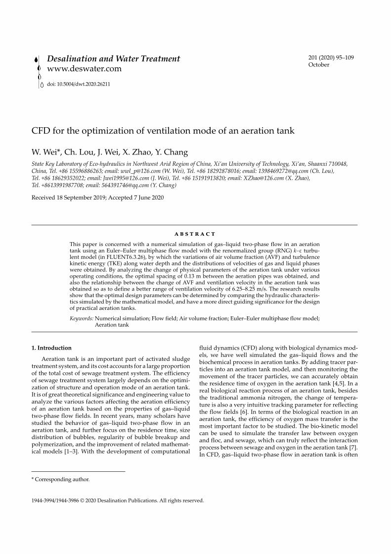
The accuracy of the simulation can be verified as fol-lows. The simulation values of liquid velocity along the two lines of x = 0.0121 m and y = 0.254 m in the character-istic cross-section of z = 0.01 m of the aeration tank under the degassing boundary conditions are compared with the

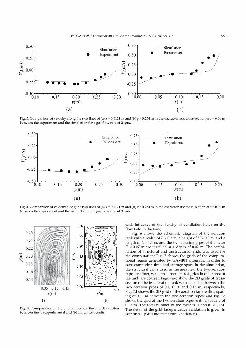
experimental ones, as shown in Figs. 3 and 4, with the gas flow rates of 2 and 3 lpm, respectively. It can be seen that, there is a little error between the simulated and experi-mental values near the wall, which may be caused by the deviation between the experimental free water surface and the simulated water surface under the degassing boundary condition; but the calculated simulation values are totally in good agreement with the experimental ones under the different aeration velocities, and reflect the distribution law of flow fields in the aeration tank. Fig. 5 shows a compar-ison between the simulated and experimental streamlines in the middle section of the aeration tank. It can be seen that the simulated streamlines are in good agreement with the experimental ones from Pfleger et al. [28] and Ali et al. [29], and the heights of the rotation center by the simula-tion and experiment are both near y = 0.17 m; therefore, the selected Euler model has the ability to capture the flow field structures of gas–liquid two-phase flow in an aeration tank.

4. Numerical simulation of an aeration tank

In running of an aeration tank, there are many factors affecting the aeration behavior, such as aeration mode, aer-ation velocity, installation depth of aeration pipe, layout of ventilation holes, and so on. In section 4 (Numerical simu-lation of an aeration tank), we will simulate the influence of different ventilation hole sizes, different aeration pipe spac-ing, and different aeration velocities on aeration behavior for a plug-flow aeration tank. TKE and volume fraction of gas are the main factors affecting the oxygen mass transfer in an aeration tank; TKE reflects the intensity of the mix-ing of gas and liquid, and volume fraction of gas reflects the concentration of oxygen in the aeration tank, therefore, the two main factors have been analyzed for the optimi-zation of the aeration tank in sections 4.2–4.5 (Influence of the spacing between aeration pipes on the flow fields in the

(a) (b)

(c)

Fig. 1. Computation domain. (a) 3D area, (b) view from side, and (c) view from top.

(a) (b)

(c)

Fig. 2. Grid of the computational domain. (a) 3D grid, (b) 2D grid of vertical section, and (c) 2D grid of cross-section.

99W. Wei et al. / Desalination and Water Treatment 201 (2020) 95–109

tank–Influence of the density of ventilation holes on the flow field in the tank).

Fig. 6 shows the schematic diagram of the aeration tank with a width of B = 0.3 m, a height of H = 0.3 m, and a length of L = 1.5 m, and the two aeration pipes of diameter D = 0.07 m are installed at a depth of 0.02 m. The combi-nation of structural and unstructured grids was used for the computation; Fig. 7 shows the grids of the computa-tional region generated by GAMBIT program. In order to save computing time and storage space in the simulation, the structural grids used in the area near the two aeration pipes are finer, while the unstructured grids in other area of the tank are coarser. Figs. 7a–c show the 2D grids of cross- section of the test aeration tank with a spacing between the two aeration pipes of 0.1, 0.13, and 0.15 m, respectively; Fig. 7d shows the 3D grid of the aeration tank with a spac-ing of 0.13 m between the two aeration pipes; and Fig. 7e shows the grid of the two aeration pipes with a spacing of 0.13 m. The total number of the meshes is about 310,224.The detail of the grid independence validation is given in section 4.1 (Grid independence validation).

(a) (b)

Fig. 3. Comparison of velocity along the two lines of (a) x = 0.0121 m and (b) y = 0.254 m in the characteristic cross-section of z = 0.01 m between the experiment and the simulation for a gas flow rate of 2 lpm.

(a) (b)

Fig. 4. Comparison of velocity along the two lines of (a) x = 0.0121 m and (b) y = 0.254 m in the characteristic cross-section of z = 0.01 m between the experiment and the simulation for a gas flow rate of 3 lpm.

(a) (b)

Fig. 5. Comparison of the streamlines on the middle section between the (a) experimental and (b) simulated results.

W. Wei et al. / Desalination and Water Treatment 201 (2020) 95–109100

4.1. Grid independence validation

Poor grid quality will easily lead to divergence of the calculation, or lead to less accuracy of simulation results; therefore, the generation of high-quality grid for the whole aeration tank is a very important task. Because the ventila-tion hole is much smaller compared with the whole testing model region, and the flow field near the ventilation hole has a greater influence on the whole flow field, an appropriate grid density and a high-quality grid near the ventilation holes need to be required. In the generation of grid, the whole aer-ation tank region is divided into two blocks, which use struc-tured and unstructured meshes, respectively. The region near

the ventilation hole is separated into unstructured meshes, and the rest are structured meshes.

Different mesh densities also have a greater influence on the discretization error; the smaller the mesh density is, the more detailed information is captured by a mathematical model, and the smaller is the error of equation discretiza-tion. However, over-dense meshes require much computing time and produce more truncation errors. Therefore, it is necessary to quantitatively estimate the mesh densities and grid quality, considering both the calculation cost and the accuracy of the calculation results. If the deviation of the simulation results is so smaller that it can be neglected in a certain range of number of meshes, the grid is independent,

(a) (b) Fig. 6. Schematic diagram of the aeration tank: (a) total body of the tank and (b) view from side.

(a) (b) (c)

(d) (e)

0 0.1 0.2 0.30

0.1

0.2

0.3

y (m)

z(m

)

0 0.1 0.2 0.30

0.1

0.2

0.3

y (m)

z(m

)

0 0.1 0.2 0.30

0.1

0.2

0.3

z(m

)

y (m)

Fig. 7. Grids of the computational region: 2D grids of cross-section with a spacing of aeration pipes of (a) 0.1 m, (b) 0.13 m, and (c) 0.15 m, (d) 3D grid of the tank with a spacing of aeration pipes of 0.13 m, and (e) 3D grid of the aeration pipes with a spacing of 0.13 m.

101W. Wei et al. / Desalination and Water Treatment 201 (2020) 95–109

and the numerical simulation results will be reliable. The geometric parameters of the testing aeration tank are shown in Table 1.

Three different numbers of grids of the tank in Table 2 are used for the grid independence validation under the same simulation method and the same boundary and ini-tial conditions, as shown in Table 3. After the calculations about grid-independence have been finished, an appro-priate range of mesh number can be determined to reduce the error of simulation results caused by mesh density. To quantitatively compare the influence of different grid den-sities on the simulation results, the average velocity over cross-sections along z-axis was selected to be compared.

Fig. 8 shows the variations of average velocity of liq-uid over cross-sections along z-axis under three different grid densities (Grid 1, Grid 2, and Grid 3). It can be seen that the grid density has a greater influence on the change of simulated physical parameters; the simulation results of Grid 1 are obviously different from that of Grid 2, but the simulation results of Grid 2 are nearly the same with that of Grid 3, which shows that Grid 2 of 310,224 meshes meets a grid independent solution. Therefore, Grid 2 was used in the following simulation in the aeration tank under dif-ferent working conditions.

4.2. Influence of the spacing between aeration pipes on the flow fields in the tank

In the design of an aeration tank, a better spacing between aeration pipes should be defined. The aeration tank model consists of a box and two aeration pipes; the ventila-tion holes on the aeration pipes are symmetrically and evenly distributed. Here, the influence of three different spaces, 0.1, 0.13, and 0.15 m, between aeration pipes, on the flow fields in the tank was analyzed, with the other parameters fixed. Figs. 9a–c show the distributions of velocity value along a line at x = 0.3, 0.6, 0.9, and 1.2 m in the plane of z = 0.075 m, from which we can see that the distributions of velocity value are evenly distributed along the flow direction, the flow velocity values near each ventilation hole are basically the same, which indicates that the calculations in the whole region have reached a stable state. Due to the cause by the influence of inlet flow direction, the distributions of veloc-ity value along the line and near water entrance has a little difference from each other for the three spaces between the aeration pipes. Fig. 9 gives a brief analysis of the flows in the aeration tank, and shows that the flows in the aeration tank are a basically symmetrical distribution.

In order to further explain the change of flow fields due to different spaces between the aeration pipes, the varia-tions of gas volume fraction and TKE along water depth are analyzed in Figs. 10 and 11, respectively. Fig. 10 shows the variation of volume fraction of gas, and Fig. 11 shows the change of TKE along the water depth under three different spaces: 0.1, 0.13 and 0.15 m of aeration pipes, respectively.

Fig. 10 shows that the variations of volume fraction of gas phase are basically the same along the water depth under the three spaces between the two aeration pipes, which indicates that the different spaces have little effect on the change of gas volume fraction. The reason is that, the smaller size of ventilation hole makes the aeration velocity become higher and causes shorter time of air residence in the aeration tank, so that the influence of different arrange-ments of aeration pipes on the flow field is made to become small. Fig. 11 shows that the distributions of TKE are dif-ferent due to the different patterns resulted from the differ-ent spaces between the two aeration pipes, which indicates that the different spaces have an effect on the distributions of TKE. The reason is that the magnitude of TKE is closely

Table 1Geometric parameters of the aeration tank (in m)

Geometric parameters Symbols

Length L 1.5Width B 0.3Height H 0.3Effective depth of water h 0.225Water head over import weir ∇H 0.038Diameter of aeration pipe D 0.07Diameter of ventilation holes r 0.0006

Table 3Boundary conditions and mathematical model for the grid independence validation

Ventilation hole Velocity import

Top exit Pressure exitVelocity at import, m/s 10Turbulence model RNG k–ε modelMultiphase flow model Euler model

Table 2Three different grids of the tank

Grid Elements

Grid 1 198,544Grid 2 310,224Grid 3 351,558

Fig. 8. Comparison of the calculation results between different grid densities.

W. Wei et al. / Desalination and Water Treatment 201 (2020) 95–109102

related to the value of velocity so that the higher aeration velocity resulting from the smaller ventilation hole size under different spaces has greater effect on the distributions of TKE. From Fig. 11, the specific value of TKE is relatively larger with a space of 0.13 m; therefore, the behavior of aera-tion is best with a spacing of 0.13 m of aeration pipes, which is more conducive to gas–liquid mixing, and further to dif-fusion and transfer of oxygen in the aeration tank.

Figs. 12 and 13 show the variations of average veloc-ity of gas and liquid phase along z-direction, respectively, under three different spaces 0.1, 0.13 and 0.15 m of aera-tion pipes. Because the slip velocity between gas and liquid phases is very small, the variation laws of the calculated average velocity of gas and liquid phases are basically the same; in addition, near the free water surface, due to the relatively smaller hydrostatic pressure and the overflow of air, the velocity of gas phase is greater, which makes the liquid to move faster and nearly at the same velocity with gas. Because of the effect of turbulent viscosity of gas and liquid, the upward movement of gas–liquid mixture leads to the movement of its surrounding liquid. Gas and liquid mixture diffuses in planes; therefore, the closer the gas and liquid mixture runs to the water surface, the greater is the gas volume fraction. In the vicinity of the ventilation holes, the bubbles do not disperse due to the great gas spill-over velocity, and form a stable column with a relatively smaller diffusion in the horizontal direction. Gas and liquid are not

(a)

(b)

(c)

00.3

0.60.9

1.21.5

00.150.30

0.05

0.1

0.15

0.2

x (m)y (m)

wat

erve

loci

ty(m

/s)

00.3

0.60.9

1.21.5

00.150.30

0.05

0.1

0.15

0.2

x (m)y (m)

wat

erve

loci

ty(m

/s)

00.3

0.60.9

1.21.5

00.150.30

0.05

0.1

0.15

0.2

x (m)y (m)

wat

erve

loci

ty(m

/s)

Fig. 9. Distributions of liquid velocity value along a line at x = 0.3, 0.6, 0.9, and 1.2 m in the plane of z = 0.075 m under three different spaces: (a) 0.1 m, (b) 0.13 m, and (c) 0.15 m, between the two aeration pipes.

0.1 0.12 0.14 0.16 0.18 0.2 0.220

0.02

0.04

0.06

0.08

0.1

0.12d = 0.1md = 0.13md = 0.15m

R=0.6mm

z (m)

Airv

olum

efra

ction

Fig. 10. Variation of the AVF along water depth in z-direction.

0.1 0.12 0.14 0.16 0.18 0.2 0.220

0.001

0.002

0.003

0.004d=0.1md=0.13md=0.15m

z (m)

κ(m

2 /s2 )

R = 0.6mm

Fig. 11. Variation of the TKE along water depth in z-direction.

0.1 0.12 0.14 0.16 0.18 0.2 0.220

0.02

0.04

0.06

0.08

d = 0.1md = 0.13md = 0.15m

R=0.6mm

z (m)

Air

velo

city

(m/s

)

Fig. 12. Variation of the average velocity of gas phase along the z-direction.

103W. Wei et al. / Desalination and Water Treatment 201 (2020) 95–109

completely mixed, which makes the average volume frac-tion of cross section be smaller.

4.3. Influence of size of the ventilation holes on the flow fields in the tank

In section 4.2 (Influence of the spacing between aeration pipes on the flow fields in the tank), the optimum spacing was obtained as 0.13 m. In section 4.3 (Influence of size of the ventilation holes on the flow fields in the tank), we will discuss the effects of different diameters of aeration pipes on the aeration behavior with a spacing of 0.13 m between the two aeration pipes.

In section 4.2 (Influence of the spacing between aeration pipes on the flow fields in the tank), it was concluded that the excessive ventilation velocity is unfavorable to the aeration behavior; therefore, we consider enlarging the ventilation hole in the aeration pipes under the same aeration mass per unit time, and with a space of 0.13 m between the aeration pipes. The three different diameters of 1.2, 1.8, and 2.4 mm of ventilation hole, are chosen to be simulated, respectively, by which the variations of the AVF and TKE along z-direction are respectively shown in Figs. 14 and 15.

From Figs. 14 and 15, we can see that, under different sizes of ventilation holes, the changes of TKE are basically the same, that is, their difference is negligible, which indicates that the gas–liquid mixing effect inside aeration tank under the three ventilation holes is basically the same; and the gas volume fractions are different, specifically with a diameter of 1.2 mm of ventilation hole, the gas volume fraction is relatively maximum. Therefore, the comprehensive analysis shows that under the three ventilation holes, the aeration behavior is best when the diameter of ventilation hole is 1.2 mm.

4.4. Influence of different ventilation velocities on flow fields in the tank

In section 4.3 (Influence of size of the ventilation holes on the flow fields in the tank), all the analysis and discus-sion were performed under the same ventilation condition, and it was obtained that the aeration behavior is best with a diameter of 1.2 mm of the ventilation holes. In section 4.4 (Influence of different ventilation velocities on flow fields in

the tank), we change the ventilation velocity with a diame-ter of 1.2 mm of the ventilation holes to study the effect of different values of ventilation velocity on the behavior of aeration. We select a range of ventilation velocity from 1.25 to 10 m/s to be simulated. Fig. 16 shows the variation trends of the volume fraction of gas phase at different ventilation velocities of 1.25, 2.5, 3.75, 1.25, 5, 6.25, and 7.5 m/s.

As can be seen from Fig. 16, the volume fraction of gas phase varies with different ventilation velocities, but they become nearly the same when the ventilation rates are in a range of 6.25–7.5 m/s, which indicates that in this range of ventilation velocity, the aeration behaviors become almost consistent, that is, the increase of ventilation velocity will not improve the aeration behavior further obviously. In addition, the relationship between the ventilation velocity and the gas volume fraction in the aeration tank is not a sim-ple linear relationship. Based on the statistical analysis of gas volume fractions calculated at different aeration rates, the relationship between the variation of ventilation veloc-ity and the gas volume fraction in the range of aeration rate was obtained here, by which we can predict the best venti-lation velocity corresponding to the maximum of AVF. Fig. 17 shows the fitting curve for the variation of the ventilation velocity with the change of volume fraction of gas phase. The equation for the fitting curve is as follows:

0.1 0.12 0.14 0.16 0.18 0.2 0.220

0.02

0.04

0.06

0.08d = 0.1md = 0.13md = 0.15m

z (m)

wat

erve

loci

ty(m

/s) R=0.6mm

Fig. 13. Variation of the average velocity of liquid phase along the z-direction.

0.1 0.12 0.14 0.16 0.18 0.2 0.220

0.03

0.06

0.09

0.12

R=1.2mmR=1.8mmR=2.4mm

d = 0.13m

Air

volu

me

frac

tion

z (m)

Fig. 14. Variation of AVF along z-direction.

0.1 0.12 0.14 0.16 0.18 0.2 0.220

0.001

0.002

0.003

0.004R=1.2mmR=1.8mmR=2.4mm

d = 0.13m

κ(m

2 /s2 )

z (m)

Fig. 15. Distribution of TKE along z-direction.

W. Wei et al. / Desalination and Water Treatment 201 (2020) 95–109104

y x x= − + +0 0004 0 0069 0 00262. . . (18)

where x represents the ventilation velocity, and y the gas volume fraction, and when x = 8.625, the maximum of y gets to 0.0324.

We can see from Fig. 17 that, with the ventilation veloc-ity in the range of 1.25–10 m/s, in the core area of the aera-tion tank, the variation of ventilation velocity with volume fraction of gas phase follows a quadratic curve; and after the ventilation rate of 7 m/s, the change range of AVF with the increasing of ventilation velocity is very small, and when ventilation velocity equals to 8.625 m/s, the maximum of AVF gets to 0.0324. Therefore, we think that the ventilation rate of 8.625 m/s can achieve the best aeration behavior.

Fig. 18 shows the variation of TKE along water depth under different ventilation velocities in the tank at 1.25, 2.5, 3.75, 1.25, 5, 6.25, and 7.5 m/s; it can be seen that the larger the ventilation velocity is, the larger is the corresponding calculated TKE. But the difference of the distributions of TKE is small at different ventilation velocities. Compared with Fig. 17, in this range of velocity from 1.25 to 7.5 m/s, Fig. 18 shows that the TKE is less affected by ventilation velocity than AVF.

At different ventilation velocities, the corresponding calculated physical parameters are different. Table 4 shows the statistical calculated physical parameters at different ventilation velocities. The TKE and AVF have been already analyzed in detail above, so only the average velocities of liquid and gas phases are analyzed here for these ventilation velocities of 1.25, 2.5, 3.75, 1.25, 5, 6.25, and 7.5 m/s. From Table 4, it can be seen that with the increase of ventilation velocity, the average velocities of gas and liquid phases increase, and the larger the ventilation velocity is, the more obvious is the difference of velocity between the gas and liquid phases.

4.5. Influence of the density of ventilation holes on the flow field in the tank

Based on the results in Sections 4.2–4.4 (Influence of the spacing between aeration pipes on the flow fields in the tank–Influence of different ventilation velocities on flow fields in the tank), the influence of the number of ventilation

holes will be studied on the flow fields with a constant spacing of 0.12 m between the two aeration pipes.

Similar to the analysis in section 4.2 (Influence of the spacing between aeration pipes on the flow fields in the tank), the variations of gas volume fraction and TKE in a typical region are selected as analysis indexes. With the increasing of number of the ventilation holes, the aeration velocity is reduced under the same amount of aeration mass per unit time. The upward movement of liquid in the aer-ation tank is mainly caused by the aeration from ventila-tion holes; therefore, the decrease of ventilation velocity has a greater influence on the upward movement of liquid so that the average velocity of liquid phase in each horizontal cross-section is chosen as another reference variable.

Figs. 19a–c indicate a comparison of the volume frac-tion of gas between before and after increasing the number of ventilation holes, under different ventilation hole sizes, respectively, from which we can see that the distribution of air in the fluid becomes more uniform when the number of ventilation holes is increased with a constant amount of aer-ation mass per unit time.

Compared with the case of greater number of venti-lation holes, the case of smaller number forms wider air columns, which is because the relatively larger ventilation velocity caused by the smaller number of ventilation holes causes a larger fluctuation so as to make the gas columns relatively more stable and more intense near water surface;

0.1 0.12 0.14 0.16 0.18 0.2 0.220

0.03

0.06

0.09

0.12

0.15 v = 1.25m/sv = 2.5m/sv = 3.75m/sv = 5m/sv = 6.25m/sv = 7.5m/s

z (m)

Air

volu

me

fract

ion

Fig. 16. Variation of AVF at different ventilation rates.

Fig. 17. Change of AVF with ventilation velocity.

0.12 0.14 0.16 0.18 0.2 0.220

0.001

0.002

0.003

0.004v = 1.25m/sv = 2.5m/sv = 3.75m/sv = 5m/sv = 6.25m/sv = 7.5m/s

κ(m

2 /s2 )

z (m)

Fig. 18. Variation of TKE along water depth with different ventilation rates.

105W. Wei et al. / Desalination and Water Treatment 201 (2020) 95–109

after increasing the hole number, the air columns become finer, but the contact area between gas and liquid in the tank is increased so as to make air diffusion more uniform, which is more conducive to the transfer of oxygen. At the same time, we also observe that the volume fraction of gas phase near the inlet is relatively higher, which indicates that the inlet velocity has a certain effect on the diffusion of air in liquid.

The decrease of aeration velocity has a greater influence on the upward movement of liquid in the tank; therefore, in the following study, the sectional average velocity of liquid phase is selected as another reference variable. Fig. 20 shows the variation of the average liquid velocity in water-depth direction under different ventilation hole sizes.

As shown in Fig. 20, after increasing the number of venti-lation holes, the variations of the sectional average velocity of

Table 4Statistical calculated physical parameters at different ventilation velocities

Statistical calculated physical parameters at different ventilation velocities

Ventilation velocities (m/s) 1.25 2.5 3.75 5.0 6.25 7.5

VOF of gas phase (%) 1.139 1.543 2.447 2.540 2.876 2.912Average of TKE (m2/s2) 0.00113 0.00117 0.00118 0.00121 0.00122 0.00123Average of velocity of gas phase (m/s) 0.0256 0.0257 0.0262 0.0266 0.0271 0.0275Average of velocity of liquid phase (m/s) 0.00261 0.0264 0.0268 0.0271 0.0273 0.0279

(a)

(b)

(c)

Fig. 19. Comparison of the gas volume fraction between the two cases of 9 and 18 ventilation holes for different ventilation hole sizes: (a) 1.2 mm, (b) 1.8 mm, and (c) 2.4 mm.

W. Wei et al. / Desalination and Water Treatment 201 (2020) 95–109106

the liquid along water depth under different ventilation hole sizes (1.2, 1.8 and 2.4 mm) are not obviously different, which indicates that in the range of ventilation velocity correspond-ing to the increased number of ventilation holes, the change of ventilation velocity is not enough to make the liquid flow velocity have an obvious difference.

Fig. 21 shows that, under different ventilation hole sizes (1.2, 1.8 and 2.4 mm), the variation of TKE of the liquid along water depth is similar to that of the velocity of liquid phase; the variations of the calculated TKE are basically the same, and the difference can be neglected. It shows that there is no obvious difference for the turbulence in the entire aeration tank under the three different ventilation velocities.

Fig. 22 shows the variation of the calculated gas volume fraction along water depth in a typical area. Under the differ-ent ventilation hole sizes (1.2, 1.8 and 2.4 mm), the variation trends of gas volume fraction are the same, but the calcu-lated values are obviously different; that is, the smaller the ventilation hole size is, the larger is the ventilation velocity, thus the larger is the calculated gas volume fraction.

In order to more accurately describe the air distribution in the aeration tank after increasing the number of ventila-tion holes, it is necessary to conduct a more comprehensive analysis of the change of flow fields under the same size but different number of ventilation holes with a constant amount of aeration mass per unit time. Figs. 23a–c show the comparison of the variations of gas volume fraction along water depth between the initial and increased number of ventilation holes under a diameter of 1.2, 1.8, and 2.4 mm of ventilation holes, respectively. From Figs. 23a–c, it can be seen that the volume fraction of gas phase increases signifi-cantly after the increasing of the ventilation hole sizes, espe-cially in the area above 0.19 m-water-depth. This is because near the free water surface, the static water pressure acting on the dissolved air decreases, and the ventilation holes are arranged densely, which makes the diffusion range of air in this area increase so as to make the volume fraction of air be larger.

From the above analysis, the flow field in the aeration tank has changed greatly with the increase of number of the ventilation holes. In order to more accurately show the change of flow fields in the aeration tank under different ventilation hole sizes, a statistical analysis of the variation of

physical parameters is made in a typical area under different diameters of 1.2,1.8, and 2.4 mm of the ventilation holes, as shown in Table 5.

From Table 5, we can see that the volume fraction of gas varies significantly with the change of ventilation hole size; the volume fraction of gas increases 31.8% at 1.2 mm-radius ventilation holes relative to 1.8 mm-radius, and increases 40.8% relative to 2.4 mm-radius, respectively; but the aver-age velocities of liquid and gas phases and TKE do not change significantly with the change of ventilation hole size. Therefore, increasing the number of ventilation holes is equivalent to increasing the contact area between gas and liquid in the tank, which is more conducive to the transfer and diffusion of oxygen, and can also change the efficiency of sewage treatment.

5. Discussions and future study plan

Numerical simulation and experimental methods are dependent upon each other; experiment is the main way to investigate a new basic phenomenon, taking a large amount of observation data as the foundation, still, the validation for a numerical simulation result must use the measured (in a prototype or a model) data. Doing numerical simula-tion in advance can obtain the preliminary results, which

Fig. 20. Variation of the liquid velocity.

z0.1 0.12 0.14 0.16 0.18 0.2 0.220

0.001

0.002

0.003

0.004R=1.2mmR=1.8mmR=2.4mm

z (m)

κ(m

2 /s2 )

Fig. 21. Variation of the TKE.

0.1 0.12 0.14 0.16 0.18 0.2 0.220

0.02

0.04

0.06

0.08R=1.2mmR=1.8mmR=2.4mm

z (m)

Air

volu

me

frac

tion

Fig. 22. Variation of the AVF with different radius of ventilation holes.

107W. Wei et al. / Desalination and Water Treatment 201 (2020) 95–109

can make the corresponding experiment plan be more purposeful, and often reduces the number of systematical experiments; therefore, it is much useful for the design of experimental device [30].

Here, an experimentally validated numerical sim-ulation method has been used to study influences of the spacing between aeration pipes, and size and number of ventilation holes in the aeration pipes on the variation of aeration behavior under the same discharge of aeration mass per unite time. Next, further study will be done to validate the test model made of organic glass by an exper-imental method. Acoustic Doppler velocimetry (ADV) will be used to measure velocities of the test model under the

various working conditions. The measured velocities can be further compared with the simulation results, by which the reliability of the simulation results can be validated. After validating the CFD model, it can predict the flow fields in aeration tanks, and the predicted results can be used to optimize the aeration tanks.

The real motion in the aeration tank is the mixture of gas, solid, and liquid phases, but here it was simplified as a gas–liquid two-phase flow; to obtain simulation results close to the real motion state, detailed simulation, and experimental studies are further needed. The flow in the aeration tank includes biochemical reactions; therefore, it has some limitations to study only from the perspective of

(a) (b)

(c) Number of vents in each pipe=9, Number of vents in each pipe=18

Fig. 23. Comparison of AVF with different radii of the ventilation holes: (a) 1.2 mm, (b) 1.8 mm, and (c) 2.4 mm.

Table 5Physical parameters for the case of different radii (r) of ventilation holes

Physical parameters for the case of radii of 1.2, 1.8, and 2.4 mm

Physical parameters

Volume fraction of gas phase (%)

Average velocity of gas phase (m/s)

Average velocity of water phase (m/s)

Average value of TKE (m2/s2)

1.2 mm-radius 1.389 0.261 0.256 0.001131.8 mm-radius 1.054 0.247 0.252 0.001172.4 mm-radius 0.986 0.251 0.257 0.00118

W. Wei et al. / Desalination and Water Treatment 201 (2020) 95–109108

flow fields. The results of the flow field research can provide some preliminary bases for the study of the combination of flow field and biological field in the future. In the real motion state of bubbles plume, the movement of bubbles in water results in coalescence and fragmentation to a certain extent; therefore, the interaction between bubbles and water needs to be further studied.

6. Conclusions

A plug-flow aeration tank was simulated by using the Euler multiphase flow model combined with the RNG k–ε turbulence model, by which the variations of AVF and TEK along water depth, and the distribution of velocities of gas and liquid phases were obtained. According to the principle of oxygen transfer, the AVF and TKE are the main analysis indexes to evaluate the aeration behavior.

The influences of spacing between the aeration pipes, and the size and number of ventilation holes in the aera-tion pipes on the variation of aeration behavior were sim-ulated under the same discharge of aeration mass per unite time. The optimum spacing between the aeration pipes was defined as 0.13 m; and with a constant amount of aeration mass per unit time, the size and number of ventilation holes influence the value of aeration velocity; that is, the larger the aeration velocity is, the larger is the AVF of the simulated gas phase, the more turbulent is the flow, and the better is the aeration behavior. However, the too higher aeration velocity of 10 m/s is not conducive to the operation of the aeration tank.

In addition, taking the ventilation velocity as an inde-pendent variable and fixing other conditions, the relation-ship between the changes of AVF and ventilation velocity in the aeration tank was obtained by the simulation results, from which it can be seen that the AVF does not increase significantly when the ventilation velocity is above 6.25 m/s; therefore, and the optimal range of ventilation velocity from 6.25 to 8.625 m/s was defined. Using the relationship, we can predict the best ventilation velocity corresponding to the maximum of AVF.

Acknowledgment

Financial support of this study was from the National Natural Science Foundation of China (Grant No. 51578452 and No. 51178391) and the scientific research projects of Shaanxi Province (2020SF-354, 2016GY-180, 15JS063).

Symbols

d — Spacing between aeration pipes, mC1ε, C2ε — Model parameters in Eq. (16)Cμ — Model parameter in Eq. (17) with a value of

0.085

Fq — External volume force, N

F qlift , — Lift force, N

Fvm q, — Virtual mass force, Nk — Turbulent energy, m2/s2

mpq — Mass transfer from p to q phasemqp — Mass transfer from q to p phase

P — Pressure shared by all phases, kg/(m × s2)Gk,q — Turbulence production of q phase in Eq. (15)

and (16)S — Parameter for computing C1εSi,j — Parameter for computing C1ε

Rqp ,

Rpq — Interaction force between p and q phases, Nui, uj — Velocity components of vm, m/s v vpq qp, — Relative velocities of between p and q phases,

m/svq — Velocity of q phase, m/svp — Velocity of p phase, m/s

Greek letters

αq — Volume fraction of q phaseβ — Constant of 0.015 for computing C1εε — Turbulent energy dissipation rate, m2/s3

η — Parameter for computing C1εη0 — Constant of 4.38 for computing C1ελq — Volume viscosity of q phaseμ — Molecular kinematic viscosity, kg/(m × s)μq — Shear force viscosity of q phase, kg/(m × s)ρq — Physical density of q phase, kg/m3

σk — Model parameter in Eq. (15) with a value of 0.7197

σε — Model parameter in Eq. (16) with a value of 0.7197

τ — Pressure-strain tensor of q phase, kg/(m × s2)

Subscripts

i,j — Direction, i = 1, 2, and 3; j = 1, 2, and 3p — p phaseq — q phasek — Turbulent energyε — Turbulent energy dissipation ratev — Velocityvm — Virtual mass force of a phase

Abbreviations

AVF — Air volume fractionADV — Acoustic Doppler velocimetryCFD — Computational Fluid Dynamics FVM — Finite volume methodRe — Reynolds numberRNG — Renormalized groupSIMPLE — Semi-implicit method for pressure-linked

equationsTKE — Turbulent kinetic energyVOF — Volume of fluid

References[1] A.V. Kulkarni, S.V. Badgandi, J.B. Joshi, Design of ring and

spider type spargers for bubble column reactor: experimental measurements and CFD simulation of flow and weeping, Chem. Eng. Res. Des., 87 (2009) 1612–1630.

[2] N.A. Kazakis, A.A. Mouza, S.V. Paras, Experimental study of bubble formation at metal porous spargers: effect of liquid

109W. Wei et al. / Desalination and Water Treatment 201 (2020) 95–109

properties and sparger characteristics on the initial bubble size distribution, Chem. Eng. J., 137 (2008) 265–281.

[3] B. Xiao, F. Zhang, G. Rong, Influence of the bubble size on numerical simulation of the gas-liquid flow in aeration tanks, China Environ. Sci., 32 (2012) 2006–2010.

[4] M. Gresch, M. Armbruster, D. Braun, W. Gujer, Effects of aeration patterns on the flow field in wastewater aeration tanks, Water Res., 45 (2011) 810–818.

[5] E.M. Cachaza, M.E. Díaz, F.J. Montes, M.A. Galán, Unified study of flow regimes and gas holdup in the presence of positive and negative surfactants in a non-uniformly aerated bubble column, Chem. Eng. Sci., 66 (2011) 4047–4058.

[6] M. Ahnert, V. Kuehn, P. Krebs, Temperature as an alternative tracer for the determination of the mixing characteristics in wastewater treatment plants, Water Res., 44 (2010) 1765–1776.

[7] Y. Le Moullec, C. Gentric, O. Potier, J.P. Leclerc, CFD simulation of the hydrodynamics and reactions in an activated sludge channel reactor of wastewater treatment, Chem. Eng. Sci., 65 (2010) 492–498.

[8] C.L. Yang, Study on Screw Aeration Equipment by Numerical Calculation of Gas-Liquid Two-Phase Flow and Experiment, PHD Thesis, Beijing University of Chemical Technology, Beijing, China, 2011.

[9] J. Wang, Numerical Simulations of Effects of Thermal Stratification and Water Depth on Flow Around Water-Lifting Aerator, PHD Thesis, Xi’an University of Architecture and Technology, Xi’an, China, 2010.

[10] P. Cheng, Numerical Simulation and Experimental Investigation of Quad-Nozzle Jet Aerator Performance, PHD Thesis, Chongqing University, Chongqing, China, 2009.

[11] B.L. Smith, On the modelling of bubble plumes in a liquid pool, Appl. Math. Model., 22 (1998) 773–797.

[12] N.G. Deen, T. Solberg, B.H. Hjertager, Large eddy simulation of the gas-liquid flow in a square cross-sectioned bubble column, Chem. Eng. Sci., 56 (2001) 6341–6349.

[13] C. Labordeboutet, F. Larachi, N. Dromard, O. Delsart, D. Schweich, CFD simulation of bubble column flows: Investigations on turbulence models in RANS approach, Chem. Eng. Sci., 64 (2009) 4399–4413.

[14] N. Yang, Z.Y. Wu, J.H. Chen, Y.H. Wang, J.H. Li, Multi-scale analysis of gas-liquid interaction and CFD simulation of gas-liquid flow in bubble columns, Chem. Eng. Sci., 66 (2011) 3212–3222.

[15] T.Y. Amiri, J.S. Moghaddas, Y. Moghaddas, A jet mixing study in two phase gas-liquid systems, Chem. Eng. Res. Des., 89 (2011) 352–366.

[16] E.B Ni, M. Boucker, B.L. Smith, Euler-Euler large eddy simulation of a square cross-sectional bubble Column using the Neptune CFD Code, Sci. Technol. Nucl. Install., 2009 (2009) 1–8.

[17] B.A. Ali, S. Pushpavanam, Analysis of unsteady gas-liquid flows in a rectangular tank: comparison of Euler-Eulerian and

Euler-Lagrangian simulations, Int. J. Multiphase Flow, 37 (2011) 268–277.

[18] W.L. Wei, Y.L. Liu, Theory of Multiphase Flow Simulation with Applications in Wastewater Treatment Engineering, 1st ed., Xi’an Shanxi Science and Technology Publishing House, Xi’an, City, China,2016.

[19] B. Shean, K. Hadler, S. Neethling, J.J. Cilliers, A dynamic model for level prediction in aerated tanks, Miner. Eng., 125 (2018) 140–149.

[20] M. Terashima, M. So, R. Goel, H. Yasui, Determination of diffuser bubble size in computational fluid dynamics models to predict oxygen transfer in spiral roll aeration tanks, J. Water Process Eng., 12 (2016) 120–126.

[21] R. Herrmann-Heber, S.F. Reinecke, U. Hampel, Dynamic aeration for improved oxygen mass transfer in the wastewater treatment process, Chem. Eng. J., 386 (2020) 1–26, doi: 10.1016/j.cej.2019.122068.

[22] A.A. Alkhalidi, H.B. Al Ba’ba’a, R.S. Amano, Wave generation in subsurface aeration system: a new approach to enhance mixing in aeration tank in wastewater treatment, Desal. Water Treat., 57 (2016) 27144–27151.

[23] S. Becker, A. Sokolichin, G. Eigenberger, Gas-liquid flow in bubble columns and loop reactors: Part II. Comparison of detailed experiments and flow simulations, Chem. Eng. Sci., 49 (1994) 5747–5762.

[24] G. Hu, I. Celik, Eulerian-Lagrangian based large-eddy simulation of a partially aerated flat bubble column, Chem. Eng. Sci., 63 (2008) 253–271.

[25] H.R. Bravo, J.S. Gulliver, M. Hondzo, Development of a commercial code-based two-fluid model for bubble plumes, Environ. Modell. Softw., 22 (2007) 536–547.

[26] L. Schiller, L. Naumann, A drag coefficient correlation, Z. Ver. Dtsch. Ing., 77 (1935) 318–320.

[27] W.-l. Wei, H.-c. Dai, Turbulence Model Theory and Engineering Applications, Shanxi Science Technology Press, Xi’an City, China, 2006.

[28] D. Pfleger, S. Gomes, N. Gilbert, H.-G. Wagner, Hydrodynamic simulations of laboratory scale bubble columns fundamental studies of the Eulerian-Eulerian modelling approach, Chem. Eng. Sci., 54 (1999) 5091–5099.

[29] B.A. Ali, C.S. Kumar, S. Pushpavanam, Analysis of liquid circulation in a rectangular tank with a gas source at a corner, Chem. Eng. J., 144 (2008) 442–452.

[30] W. Wei, Y. Liu, B. Lv, Numerical simulation of optimal submergence depth of impellers in an oxidation ditch, Desal. Water Treat., 57 (2016) 8228–8235.