CFD Analysis of the Cool Down Behaviour of Molten Salt Thermal

Proceedings of the ASME 2nd International Conference on Energy Sustainability ES2008

August 10-14, 2008, Jacksonville, Florida, USA

ES2008-54101

CFD ANALYSIS OF THE COOL DOWN BEHAVIOUR OF MOLTEN SALT THERMAL STORAGE SYSTEMS

Jan Schulte-Fischedick* German Aerospace Center (DLR), Institute of

Technical Thermodynamics

*currently at SCHOTT-Solarthermie GmbH, Erich-Schott-Straße 14, 95 666 Mitterteich,

Germany email: [email protected]

Rainer Tamme German Aerospace Center (DLR), Institute of

Technical Thermodynamics, Pfaffenwaldring 38/40, 70569 Stuttgart,

Germany, email: [email protected]

Ulf Herrmann Flagsol GmbH, Agrippinawerft 22,

D-50678 Koeln, Germany, email: [email protected]

Proceedings of ES2008 Energy Sustainability 2008

August 10-14, 2008, Jacksonville, Florida USA

ES2008-54101

ABSTRACT CFD analysis has been conducted to obtain information on

heat losses, velocity and temperature distribution of large molten salt Thermal Energy Storage (TES) systems. A two-tank 880 MWh storage system was modeled according to the molten salt TES containment design proposed for the 50 MWel commercial parabolic trough solar thermal power plants in Spain.

Heat losses were established using the Finite Element Method (FEM), and used to determine the boundary conditions for the subsequent two- and three-dimensional Computational Fluid Mechanics (CFD) calculations. The investigations reveal that a high heat loss flux occurs at the lower edges of the salt storage tanks (between side wall and bottom plate). Thus the maximum temperature difference can be found at this location, resulting in the onset of local solidification within 3.25 days in the case of the empty cool tank. As a consequence, the detailed design of the lower edge has a large impact on both the overall heat losses and the period until the onset of local solidification.

INTRODUCTION

As a result of the revival of concentrated solar power plant technology, TES has obtained large attention in research and development. Several options are currently being investigated.

In cases where commercial parabolic trough plants operated with synthetic oil are equipped with a TES system, the two-tank molten salt sensible heat storage system is usually selected. Its feasibility was proven in the frame of the Solar Two project, in which a molten salt TES was operated as part of a tower power plant for 14 months. This demonstration plant used 1400 t of a binary salt mixture, composed of 60 wt.-% NaNO3 and 40 wt.-% KNO3, enough for 3 h full-load operation of the 10 MWel steam cycle [1].

In the case of the first two commercial trough power plants in Spain – ANDASOL-1 and ANDASOL-2 – a TES system is projected, allowing for 7.5 h full-load operation of the 50 MWel turbo set. During charging salt is taken from the cold tank, heated in heat exchangers and stored in the hot tank. The heat necessary for the charging process is taken from thermo-oil bypassing the steam cycle. During discharging this process is reversed. A salt storage mass of 28000 t is required to reach the demanded capacity of 7.5 hours full-load operation of the power plant. [2]

As this amount is twenty times larger than in the case of the Solar Two system important design aspects arise. Especially the fluid dynamic behaviour of large liquid reservoirs and its influence on the cool down times until the onset of local solidification need consideration.

1 Copyright © 20xx by ASME

Copyright © 2008 by ASME

The principal flow inside enclosures was investigated by Evans et al. [3], who used a glycerine-water mixture heated from the side wall of a cylindrical tank. They found, that the resulting vertical (upward) flow is confined to a small boundary zone near the heated wall, while the downward stream spreads over a large volume in the centre of the tank. Papanicolaou and Belessiotis [4] investigated numerically the cool down behaviour of large underground storage tanks. Filled initially with hot (60 °C) water, the tank was left to interact with the surrounding soil (-10 °C). A similar velocity distribution like in the case of Evans et al. was found, but with reversed direction, as the investigated problem was a cool down process. With increasing time they observed a transition from a convection into a conduction based regime. The main phases are successively (i) sidewall boundary formation, (ii) built-up of stratification, and (iii) final smoothing out of remaining disturbances towards a final equilibrium state.

Unfortunately, no general empirical solutions exist for the heat transfer in enclosures. Several equations have been proposed that are restricted to special ranges of aspect ratios, Rayleigh and Prantl numbers and are limited to special heating or cooling configurations [5]. The design of most practical applications is thus left to the application of Computational Fluid Dynamics (CFD) [6].

The presented CFD calculations were conducted to establish a basic knowledge of the fluid mechanical effects to evaluate ruling the cool down behaviour of the molten salt. This has to be recognized as a precondition for improving the tank design. As the heating system projected for the salt storage tanks is only able to raise the temperature of molten salt, but not to re-melt large volumes of solid salt economically, any freezing has to be avoided. Thus it is important to know the locations where local freezing has to be expected as well as the cool down times until the onset of local solidification. The former shall be the basis for the detailed design of insulation. The latter is used to determine an appropriate operation strategy during shutdown periods.

BASIC CONCEPT OF THE PROJECTED TWO-TANK TES

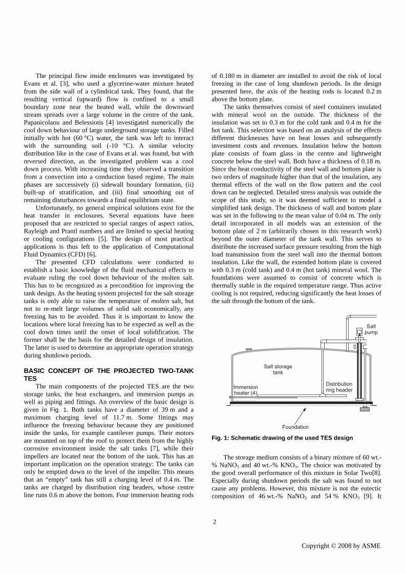
The main components of the projected TES are the two storage tanks, the heat exchangers, and immersion pumps as well as piping and fittings. An overview of the basic design is given in Fig. 1. Both tanks have a diameter of 39 m and a maximum charging level of 11.7 m. Some fittings may influence the freezing behaviour because they are positioned inside the tanks, for example cantilever pumps. Their motors are mounted on top of the roof to protect them from the highly corrosive environment inside the salt tanks [7], while their impellers are located near the bottom of the tank. This has an important implication on the operation strategy: The tanks can only be emptied down to the level of the impeller. This means that an “empty” tank has still a charging level of 0.4 m. The tanks are charged by distribution ring headers, whose centre line runs 0.6 m above the bottom. Four immersion heating rods

of 0.180 m in diameter are installed to avoid the risk of local freezing in the case of long shutdown periods. In the design presented here, the axis of the heating rods is located 0.2 m above the bottom plate.

The tanks themselves consist of steel containers insulated with mineral wool on the outside. The thickness of the insulation was set to 0.3 m for the cold tank and 0.4 m for the hot tank. This selection was based on an analysis of the effects different thicknesses have on heat losses and subsequently investment costs and revenues. Insulation below the bottom plate consists of foam glass in the centre and lightweight concrete below the steel wall. Both have a thickness of 0.18 m. Since the heat conductivity of the steel wall and bottom plate is two orders of magnitude higher than that of the insulation, any thermal effects of the wall on the flow pattern and the cool down can be neglected. Detailed stress analysis was outside the scope of this study, so it was deemed sufficient to model a simplified tank design. The thickness of wall and bottom plate was set in the following to the mean value of 0.04 m. The only detail incorporated in all models was an extension of the bottom plate of 2 m (arbitrarily chosen in this research work) beyond the outer diameter of the tank wall. This serves to distribute the increased surface pressure resulting from the high load transmission from the steel wall into the thermal bottom insulation. Like the wall, the extended bottom plate is covered with 0.3 m (cold tank) and 0.4 m (hot tank) mineral wool. The foundations were assumed to consist of concrete which is thermally stable in the required temperature range. Thus active cooling is not required, reducing significantly the heat losses of the salt through the bottom of the tank.

Salt storagetank

Distributionring header

Immersionheater (4)

Foundation

Saltpump

Fig. 1: Schematic drawing of the used TES design

The storage medium consists of a binary mixture of 60 wt.-% NaNO3 and 40 wt.-% KNO3. The choice was motivated by the good overall performance of this mixture in Solar Two[8]. Especially during shutdown periods the salt was found to not cause any problems. However, this mixture is not the eutectic composition of 46 wt.-% NaNO3 and 54 % KNO3 [9]. It



solidifies within a temperature range between 240 °C and 222 °C in the case of pure salts. Even a localised solidification is considered a major risk, because it may have a significant impact on the flow characteristics and thereby on the operation of the TES. Therefore the avoidance of any local solidification was the goal of the design. The simulations presented in the following aim to clarify, how much time remains from the beginning of a standstill of the power plant until the onset of freezing which was defined by a lower temperature limit of 240 °C.

The TES layout described above raises the full-load operation from 2000 to 3600 hours per year [2]. The specific investment cost to be expected amounts to approximately 30 - 40 US$/kWhth [10].

DESCRIPTION OF THE MODELS USED The reported investigations were conducted with different

models using the Finite Element Method (FEM), and both two- and three-dimensional Computational Fluid Dynamics. The principal investigations in this work were done with the help of the CFD-models. However, due to limitation in computational resources a detailed reproduction of the problem in 3D-CFD was not possible. In addition the used FEM-package allows adding self-programmed functions enabling extensive investigations of the different heat transfer modes. Thus the FEM model was used to establish the heat losses distinguished in locations (side wall, cap and into the soil). These founded the basis for the arrangement of the appropriate boundary conditions of the CFD models. It has to be stressed that FEM and CFD models are not conjugated, but form complete problems fully satisfying energy conservation and temperature continuity.

The models are described in the following. The fluid properties as well as the heat conductivity cannot be presented here due to a non-disclosure agreement. FEM model

All FEM calculations were conducted with the commercially available software package Ansys 8.1 and its internal programming language APDL facilitating parameters studies. The FEM model for the heat loss calculation comprises all solid parts of the storage tank except the concrete foundation. This includes the steel wall and the different insulation materials of bottom, side, and cover. The respective heat loss fluxes were integrated into the model by using convective boundary conditions. Self-programmed additions to the model, based on empirical equations, allowed to reproducing the different types of convection inside and outside the tank. Thus the effects of different temperatures were correctly implemented into the FEM model.

Fig. 2: schematic drawing of the outer bottom region of the 2D- models (both FEM and CDF) with included convective and conductive heat transfer modes. Not included is the heat transfer over the cap (radiative heat exchange from the salt surface to the cap, conduction through the cap and mixed convection on the outer surface).

Inside the tank, the molten salt is driven by buoyancy forces. For the case of natural convection within enclosures no general equations are available. Thus the heat loss through the wetted part of the circumferential side wall was assumed to be the main drive of the salt motion. This hypothesis was later confirmed by CFD calculations. Based on a comparative evaluation of equations describing the natural convection along a vertical, cylindrical wall, the choice fell on the one proposed by Aydin et al. [11]. It is applicable for both laminar and turbulent flows within a large range of Rayleigh-numbers from 10 to 1016 and Prantl-numbers from 10-3 to 103. However, during the course of the calculations (both FEM and CFD), the temperature difference in the boundary layer at the side wall was found to be as low as approximately 1 K due to the thick insulation. Thus any error in this equation has only a negligible effect on the heat loss determination. The heat transfer coefficients obtained were also used to derive the wall temperatures at the bottom of the tank and the surface of the liquid salt.

Besides the convectional heat transfer from the molten salt to the steel wall, heat is transferred via radiation exchange between the salt surface and the non-wetted areas of the salt wall and cover. This was integrated in the FEM model by the matrix method included in Ansys, conducting an identification of the radiation form factors of the corresponding areas via ray-tracing prior to thermal calculation.

Outside the tank, the heat transfer to the ambient air is ruled by mixed convection, both forced (wind) and natural. These effects were accounted for by equations recommended by [12] for the case of a vertical cylinder. The integration of the wind allowed for additional investigations on its effect on the



heat losses, demonstrating a parabolic rule. However, these investigations are beyond the scope of this report. In the following, a standard wind velocity of 1 m/s was taken.

Heat conduction into the concrete foundation and the soil was described by conduction into a semi-infinite body [12]. This is a simplified assumption that may not reproduce the true heat flux deviation at the outer boundary of the tank. However, this was chosen to keep the required computational resources low while maintaining the principal effects. 2D-CFD model

All CFD calculations, both two- and three-dimensional, were solved with the commercial software package Fluent 6.1.22. Fluent does not offer a programming language like APDL, so all models had to be built up separately by the graphical pre-processor Gambit.

Two-dimensional CFD calculations were conducted by employing an axisymmetric cross-section of the tank. This includes salt and all solids, except for the concrete foundation and all non-wetted areas of the wall and the cover. By omitting the latter, an explicit modeling of the radiation exchange between the salt surface and the steel cover was replaced by boundary conditions described later. This procedure saves one order of magnitude of calculation expenditures. On the other hand, it neglects the heat conduction along the steel container, amounting for approximately 0.6 % of the total heat losses. This is clearly negligible compared to typical errors of CFD calculations, being in the range of 20-30 % [13].

The heat transfer at the outside of the solid parts was not modeled explicitly, but represented by the same boundary conditions already used in the FEM model. In Fluent, this is possible by applying a constant temperature, a constant heat flux or a convective boundary condition. The latter was used in all cases as it enables temperature dependent heat fluxes. In the case of the modeled part of the tank wall, the heat transfer coefficients were calculated via empirical correlations for mixed convection [12] using the mean side wall temperature obtained from the FEM calculations. The use of a mean temperature neglects temperature variations along the outer surface. However, the variation along the side wall was found to be in an interval of 3 K around the mean temperature of 55°C. The heat transfer is nearly solely dominated by the thick insulation, so that any deviation from the mean temperature has only a negligible effect on the heat transfer coefficients.

The heat conduction equation for the heat flux into the soil was re-arranged to fit into the convective boundary scheme of Fluent. In the case of the non-wetted (and not explicitly modeled) parts of the tank, the entire heat transfer from the salt surface to the ambient in terms of heat loss was identified as a function of the temperature via FEM and linearized within the temperature interval of 230 °C to 300 °C. The mean error was less than 0.5 %.

To consider the effects of different charging levels, models of the full, half-filled and empty tank (level of 0.4 m) were built. In all models the overall node density was adjusted to

consider all relevant effects. The criterion used for this adaptation was the temperature difference with increasing time. The mean temperature obtained from CFD calculations was compared to the analytically calculated result of an energy balance. In addition the minimum temperature located in the lower, outer perimeter of the tank was used to determine an optimum grid density: the node density was increased step by step until no further change in the minimum temperature was observed.

To select an optimum turbulence model, the comparison between the mean temperatures calculated via CFD and analytically via an energy balance was used. Thus it was found that in the case of the half-filled and empty tank the Realizable k-ε model gave the best results, in the case of the full tank the Standard k-ε one. 3D-CFD

The effects of the fittings on the flow and the cool down behaviour cannot be evaluated using two dimensional models. Due to reasons described later, the influence of the heating elements was of special interest. Thus a 3D-modell was developed incorporating the four elements, equally spaced along the circumference of the tank. To reduce the time of calculation, only a quarter of the tank was modeled. The intersections were coupled by periodic boundary conditions. Originally it was planned to set the corresponding heating element in the midst of the modeled quarter. However, thus the end of the heating rod was positioned near the tip of the quarter. Thus the generated geometric boundaries proved to be difficult resulting in instabilities in meshing. Alternatively, the corresponding heating element was cut in half, and each half was placed into one of the intersections of the modeled quarter.

The thermal boundary conditions were the same as in the 2D calculations.

With respect to calculation time the node density was only half of the one used in the two-dimensional case. The same approach in qualifying the grid mesh demonstrated that the used grid was not dense enough to give reliable results. Thus these calculations are not used to establish the absolute temperature difference between mean and minimum temperature, which was found directly below the heating rods (described later). Instead, the temperature difference between minimum temperatures in the region not influenced by the heating elements and in immediate vicinity of the elements was determined and superimposed on the results from the 2D-CFD investigations.

Calculations were conducted using a parallel architecture. However, computational efforts were still high, so that only the case of the half-filled tank was exemplarily calculated. Like the 2D case, the Realizable k-ε turbulence model was chosen.

RESULTS The investigation of the salt storage tanks was conducted

in three steps. As no experimental data of a comparable case



was available, a FEM model was used to establish the occurring heat loss fluxes. In the second step the behaviour of the storage medium was investigated by means of two-dimensional Computational Fluid Dynamics (CFD). Finally, the influence of the fittings attached to the tank was described by a three-dimensional CFD- model. Determination of the heat losses (FEM)

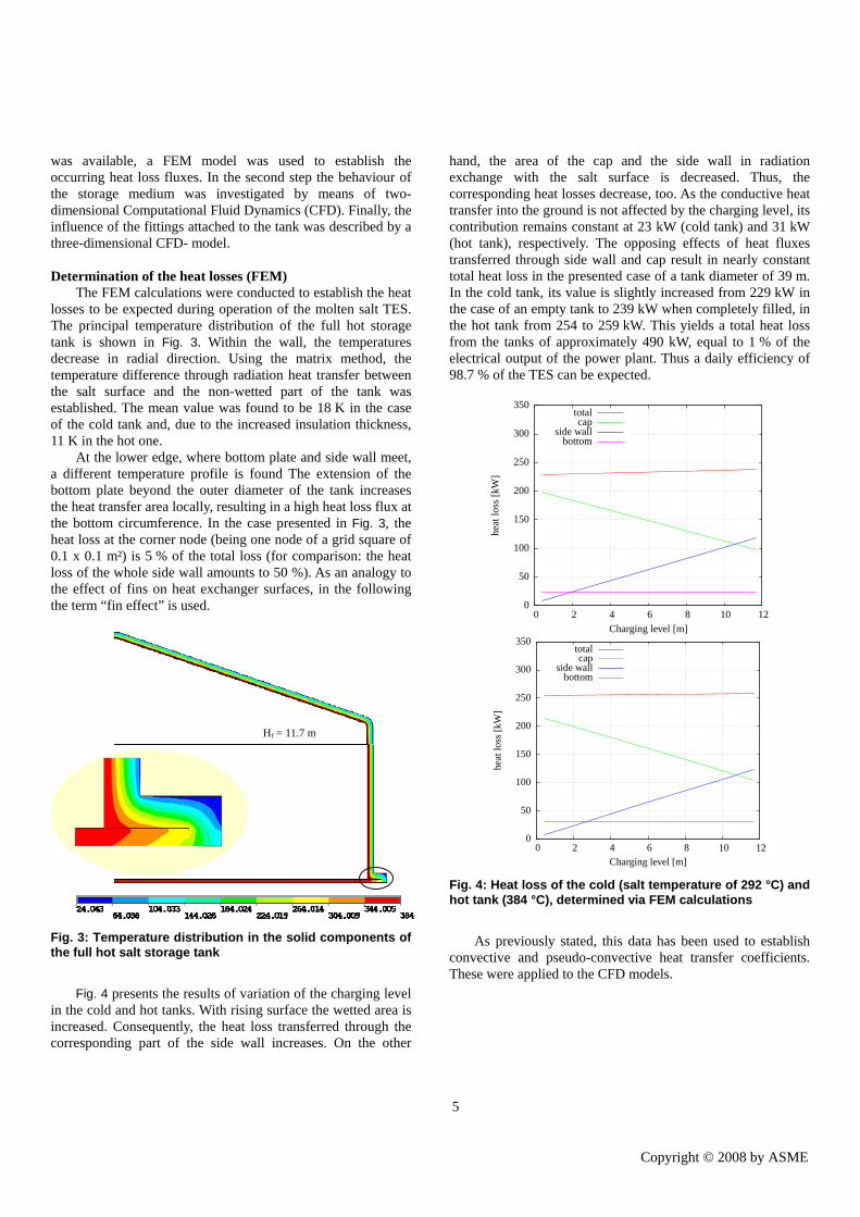
The FEM calculations were conducted to establish the heat losses to be expected during operation of the molten salt TES. The principal temperature distribution of the full hot storage tank is shown in Fig. 3. Within the wall, the temperatures decrease in radial direction. Using the matrix method, the temperature difference through radiation heat transfer between the salt surface and the non-wetted part of the tank was established. The mean value was found to be 18 K in the case of the cold tank and, due to the increased insulation thickness, 11 K in the hot one.

At the lower edge, where bottom plate and side wall meet, a different temperature profile is found The extension of the bottom plate beyond the outer diameter of the tank increases the heat transfer area locally, resulting in a high heat loss flux at the bottom circumference. In the case presented in Fig. 3, the heat loss at the corner node (being one node of a grid square of 0.1 x 0.1 m²) is 5 % of the total loss (for comparison: the heat loss of the whole side wall amounts to 50 %). As an analogy to the effect of fins on heat exchanger surfaces, in the following the term “fin effect” is used.

Fig. 3: Temperature distribution in the solid components of the full hot salt storage tank

Fig. 4 presents the results of variation of the charging level in the cold and hot tanks. With rising surface the wetted area is increased. Consequently, the heat loss transferred through the corresponding part of the side wall increases. On the other

Hf = 11.7 m

hand, the area of the cap and the side wall in radiation exchange with the salt surface is decreased. Thus, the corresponding heat losses decrease, too. As the conductive heat transfer into the ground is not affected by the charging level, its contribution remains constant at 23 kW (cold tank) and 31 kW (hot tank), respectively. The opposing effects of heat fluxes transferred through side wall and cap result in nearly constant total heat loss in the presented case of a tank diameter of 39 m. In the cold tank, its value is slightly increased from 229 kW in the case of an empty tank to 239 kW when completely filled, in the hot tank from 254 to 259 kW. This yields a total heat loss from the tanks of approximately 490 kW, equal to 1 % of the electrical output of the power plant. Thus a daily efficiency of 98.7 % of the TES can be expected.

bottomside wall

captotal

Charging level [m]

heat

loss

[kW

]

121086420

350

300

250

200

150

100

50

0

bottomside wall

captotal

Charging level [m]

heat

loss

[kW

]

121086420

350

300

250

200

150

100

50

0

Fig. 4: Heat loss of the cold (salt temperature of 292 °C) and hot tank (384 °C), determined via FEM calculations

As previously stated, this data has been used to establish convective and pseudo-convective heat transfer coefficients. These were applied to the CFD models.



Evaluation of the principal flow characteristics during cool down (2D-CFD)

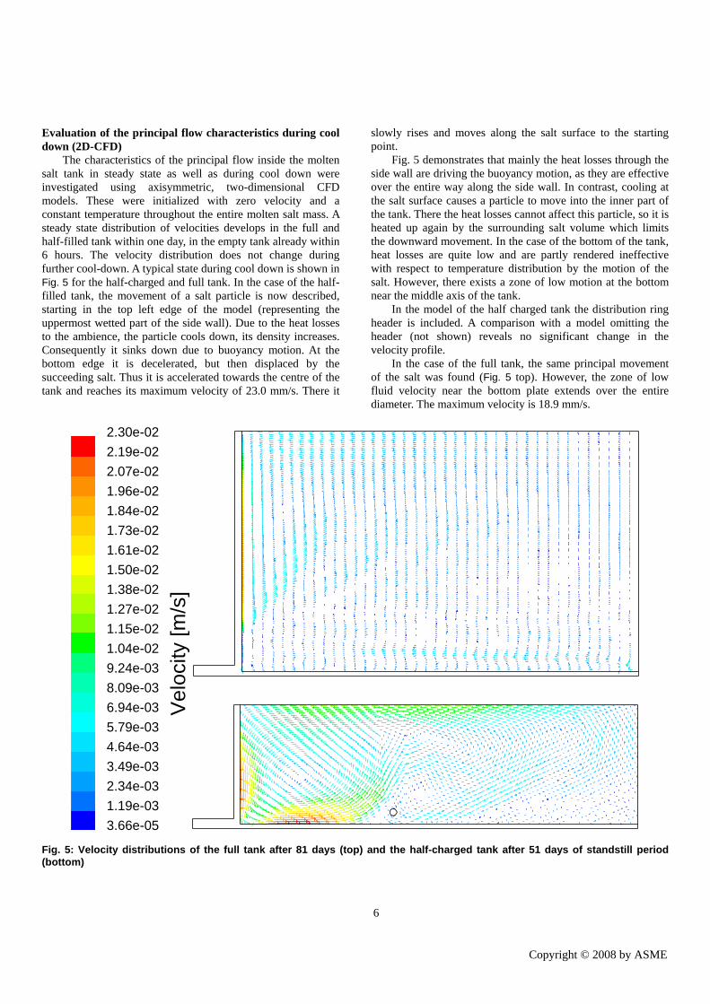
The characteristics of the principal flow inside the molten salt tank in steady state as well as during cool down were investigated using axisymmetric, two-dimensional CFD models. These were initialized with zero velocity and a constant temperature throughout the entire molten salt mass. A steady state distribution of velocities develops in the full and half-filled tank within one day, in the empty tank already within 6 hours. The velocity distribution does not change during further cool-down. A typical state during cool down is shown in Fig. 5 for the half-charged and full tank. In the case of the half-filled tank, the movement of a salt particle is now described, starting in the top left edge of the model (representing the uppermost wetted part of the side wall). Due to the heat losses to the ambience, the particle cools down, its density increases. Consequently it sinks down due to buoyancy motion. At the bottom edge it is decelerated, but then displaced by the succeeding salt. Thus it is accelerated towards the centre of the tank and reaches its maximum velocity of 23.0 mm/s. There it

slowly rises and moves along the salt surface to the starting point.

Fig. 5 demonstrates that mainly the heat losses through the side wall are driving the buoyancy motion, as they are effective over the entire way along the side wall. In contrast, cooling at the salt surface causes a particle to move into the inner part of the tank. There the heat losses cannot affect this particle, so it is heated up again by the surrounding salt volume which limits the downward movement. In the case of the bottom of the tank, heat losses are quite low and are partly rendered ineffective with respect to temperature distribution by the motion of the salt. However, there exists a zone of low motion at the bottom near the middle axis of the tank.

In the model of the half charged tank the distribution ring header is included. A comparison with a model omitting the header (not shown) reveals no significant change in the velocity profile.

In the case of the full tank, the same principal movement of the salt was found (Fig. 5 top). However, the zone of low fluid velocity near the bottom plate extends over the entire diameter. The maximum velocity is 18.9 mm/s.

2

2

2

2

2

2

2

2

3

3

3

3

3

3

3

2.30e-02

2.19e-02

2.07e-02

1.96e-02

1.84e-02

1.73e-02

1.61e-02

1.50e-02

1.38e-02

1.27e-02

1.15e-02

1.04e-02

9.24e-03

8.09e-03

6.94e-03

5.79e-03

4.64e-03

3.49e-03

2.34e-03

1.19e-03

3.66e-05

Vel

ocity

[m/s

]

Fig. 5: Velocity distributions of the full tank after 81 days (top) and the half-charged tank after 51 days of standstill period (bottom)



In the empty tank, the velocity profile is characterized by several cells of rotating salt (see streamlines at the top of Fig. 6). Like in the other cases, these cells are driven by cooling of the side wall. The velocity distribution is regular with a

maximum of 7.0 mm/s. Zones of low velocity do not occur, neither near the side wall (presented in Fig. 6 on the bottom) nor in the inner parts (not shown).

7.02e-036.67e-036.33e-035.98e-035.63e-035.28e-034.93e-034.58e-034.23e-033.88e-033.54e-033.19e-032.84e-032.49e-032.14e-031.79e-031.44e-031.09e-037.46e-043.97e-044.87e-05

Velo

city

[m/s

]

Fig. 6: Streamlines (top) and velocity distribution (bottom) after 84 hours cool down of the empty tank. Streamlines are distorted in vertical direction to fully present all details



In the following, only the half filled tank is described in detail, in the other two cases the description is confined to characteristic data.

When investigating sites where local solidification has to be expected one has to look for volumes, where low velocities appear along with high heat loss fluxes. In the half-filled tank, these can be found at the lower edge of the salt volume and at the salt surface close to the wall (see Fig. 5 on the bottom). The temperature distribution at these locations after 51 days is presented in Fig. 7. Near the bottom plate the heat loss fluxes to the ambience via the side wall and into the soil are superimposed. These are significantly increased by the fin effect. Consequently, this is the location where the lowest temperature in the entire tank occurs. After 51 days a temperature of 239 °C is reached, which is within the solidification interval.

At the salt surface close to the wall, only a low decrease in temperature can be observed. Here, the high heat loss flux results in a decrease in temperature as well. However, the corresponding particles sink quickly to the bottom of the tank due to buoyancy, resulting only in a short dwell time. Thus the temperature difference at the surface is limited in this case.

Between the two locations presented in Fig. 7, the isothermal lines are parallel to the steel surface. The mean temperature difference at the wall is 1 K, thus confirming the statement in section 0.

Beside the inspection of intermediate states, the course of temperatures was monitored during the entire calculation. The mean as well as the minimum temperatures of the half-charged and empty tank are presented in Fig. 8. As stated previously, pseudo steady state behaviour is reached one day after initialisation in the case of the half-charged tank. From this point in time onward, the relative temperature distribution does not changed any more. This is demonstrated by a constant temperature difference of 8.2 K between the minimum and the mean temperature curves. Besides CFD calculation, the mean temperature difference was calculated by an energy balance, thus allowing for an estimation of the error. This was found to be low (3 K after 51 days). Using an energy balance, a cooling rate of 0.95 K/d can be determined. Using the mean temperature of the energy balance and the temperature difference between mean and minimum temperature as obtained from CFD, the local solidification in the half filled tank was identified to start after 46 days of standstill of the power plant. In the case of the empty tank the cooling rate is 13.4 K/d, the onset of local solidification is reached within 3.5 days.

222222222222222222222

520519.5519.1518.7518.2517.8517.3516.8516.4516515.5515514.6514.2513.7513.3512.8512.3511.9511.5511

T [K]

Fig. 7: Temperature distribution at the side wall of the salt volume near the bottom plate (left) and the salt surface (right)

minimum (CFD)mean (CFD)

analytical

t [d]

Tsa

lt[◦

C]

706050403020100

300

290

280

270

260

250

240

minimum (CFD)mean (CFD)

analytical

t [d]

Tsalt

[◦C

]

543210

300

290

280

270

260

250

240

230

220

Fig. 8: Course of characteristic temperatures during cool down of the molten salt: half charged (top) and empty tank (down)

In all cases considered, the minimum temperature occurs at the lower edge. The data characterizing the cool down behavior in dependence of the charging level is summarized in

Table 1. These data demonstrates that especially the empty tank (equal to a charging level of 0.4 m) is prone to local solidification. This is based on the heat losses being nearly independent on the charging level of the tank (see Fig. 4).



Table 1: Characteristic data of the cool down behaviour of the empty, half and fully charged tank: maximum temperature difference ΔTmax, mean cooling rate and onset of solidification at the lower edge in the region not influenced by the heating elements and in immediate vicinity of the elements; the data written in italics is based on the assumption of a temperature distribution comparable to the half-charged tank.

Charging level

Charging level

[m]

ΔTmax [K]

Cooling rate [K/d]

Onset of local

solidification [d] (2D-

CFD)

Onset of solidification at heating elements [d] (3D-CFD)

Empty 0.4 5.1 13.4 3.5 3.25 Half 5.85 8.2 0.95 46 43 full 11.7 10.8 0.47 87 81

Calculation of the effects of the heating elements on natural convection (3D- CFD)

Having investigated the principal behavior of the natural convection inside the storage tank, the influence of the fittings was analyzed. As the distribution ring header is a rotationally symmetric component, it was implemented in the two dimensional CFD simulation. The direct comparison between the velocity (Fig. 5 on the bottom) and temperature distribution to those obtained from the same model without header revealed that the header does not have any impact. The same has to be expected from the vertical distribution pipe as well as the pipes of the cantilever pump. The distribution pipe has a diameter comparable to the ring header. The pipes of the cantilever pumps are located in a part of the tank that exhibits streamlines mainly orientated in parallel to the pipes. Only the impeller casing may cause some turbulence, but this result in an increased mixing of the salt and consequently in reduced temperature gradients.

The case of the heating elements is different. Their axis is positioned only 0.2 m above the bottom plate near the lower edge, where the high heat loss flux due to the fin effect occurs (see section 0). Below the heating elements low velocities have to be expected, resulting in an increased temperature difference. Thus an additional model was implemented to investigate the effect of the heating elements on the temperature distribution. The results in the case of a standstill period of four days are presented in Fig. 9. As expected, the use of the projected heating element configuration results in an additional temperature difference of 3 K right below the fixture of the elements. In the previous section it was established that the temperature distribution relative to the mean temperature does not change with increasing cooling time. The cooling rate in the half charged tank was determined to be 0.95 K (Table 1), so the onset of solidification takes place after 43 days of standstill. Assuming an identical temperature difference of 3 K in the full and empty tank, the

onset of solidification has to be expected after 81 and 3.25 days respectively.

561560.6560.2559.8559.4559558.6558.2557.8557.4557556.6556.2555.8555.4555554.6554.2553.8553.4553

ZY

X

T [K

]

T = 283 °C

Tmin = 280 °C Fig. 9: Temperature distribution in the half-filled tank four days after the start of cool down.

CONCLUSIONS In the present report numerical calculations by means of

FEM and CFD were conducted to investigate the behavior of the molten salt storage medium during standstill periods. The results indicate that the charging level exerts only a marginal influence on the heat losses. Its effect on the flux through the side wall is nearly annihilated by the flux over the cap. The extension of the bottom plate necessary to meet structural requirements results in a significant increase in heat loss flux density based on the fin effect. In the presented case (extension of 2 m beyond the outer diameter of the tank) this amounts to 5 % of the total heat losses.

Consequently, the fin effect exerts a large impact on velocity and temperature distribution. The lower edge (contact area of side wall and bottom plate) is the location, where the highest temperature difference was discovered in all calculated cases (empty, half-full and full tank). This is where the onset of local solidification has to be expected. Outside the immediate vicinity of the heating elements, the following periods until the onset of local solidification were obtained: 3.5 days in the case of the empty, 46 days in the half-full and 87 days in the full tank. A three-dimensional CFD simulation revealed that in the vicinity of the heating elements an additional temperature difference of 3 K compared to the locations outside the vicinity of the elements occurs in the half-full tank. Consequently, freezing starts right below the support of the elements already after 43 days. Assuming that the same temperature difference holds for the empty and the full case, the onset at this location has to be expected after 3.25 and 81 days, respectively.

The reaction time on standstills can be regarded as sufficient in the case of full and half-full tank, but not in the empty tank. However, the case of an empty cool tank does not



appear during normal operation. If a standstill occurs, while the TES is fully charged (corresponding to an empty cool tank), there are several options to reduce the risk of freezing. However, this case might occur due to technical faults. Keeping the long demanded operation time of 25 years in mind, an emergency bypass is thus recommended, allowing e.g. an equalization of the charging levels in both tanks.

The high sensitivity of both heat losses and temperature differences on the structural design of the lower edge illuminates a seemingly contradictory statement on the heat loss: although heat loss is in principle not desired, it constitutes the driving force of the buoyancy motion. This leads to a good mixing of cool and hot salt, ensuring a homogeneous temperature distribution. Hence, large temperature differences can only evolve in areas, where a large heat loss flux density appears along with low fluid velocities. This is particularly obvious in the vicinity of the heating elements, whose support is in the influence zone of the fin effect.

Therefore, the authors recommend to thoroughly proceed the presented investigations, once the detailed tank design has been determined. This should include all support elements necessary to meet structural requirements (like support fins to resist lateral forces), as well as the detailed geometry of the insulation. Thus the optimum design can be found, offering both low heat losses and low temperature differences inside the molten salt storage medium.

ACKNOWLEDGEMENTS The authors express their gratitude to the German Federal

Ministry for the Environment, Nature Conservation and Nuclear Safety for supporting these investigations as part of the Project “ANDA F&E” (contract number 16UM0027-31). Special thanks are given to Piyawan Woratat, who contributed to the three-dimensional CFD-analysis during their internship.

REFERENCES [1] Kearney, D., Price, H., 2004, “Assessment of Thermal Energy Storage for Parabolic Trough Solar Power Plants”, Proceedings of 2004 Solar Conference, Portland Oregon, published on CD-ROM. [2] Geyer, M., Herrmann, U., Sevilla, A., Nebrera, J.A., Zamory, A.G., 2006, “Dispatchable Solar Electricity for Summerly Peak Loads from the Solar Thermal Projects ANDASOL-1 and ANDASOL-2”, Proceedings SolarPaces 2006 A4 S2, Sevilla, Spain, published on CD-ROM. [3] Evans, L.B., Reid, R. C., Drake, E. M., “Transient natural convection in a vertical cylinder“, AIChE J., 14, 2, 1968 No. 2, pp. 251-259. [4] Papanicolaou, E., Belessiotis, V., “Transient hydrodynamic phenomena and conjugate heat transfer during cooling of water in an underground thermal storage tank“, Trans. ASME, 126, 2004, pp. 84-96. [5] Keyhani, M., Kulacki, F.A., “Natural Convection in Enclosures Containing Tube Bundles”, in: Kakac, S., Aung.,

W., “Natural convection – Fundamentals and Applications”, Hemisphere Pub. Washington, 1985, pp. 330-380. [6] Cònsul, R., Rodríguez, I., Pérez-Segarra, C.D., Soria, M., “Virtual Prototyping of Storage Tanks by means of three-dimensional CFD and hHeat Transfer Numerical Simulation, Sol. Energy, 77, 2004, pp. 179-191. [7] Barth, D.L., Pacheco, J.E., Kolb, W.J., Rush, E.E., “Development of a High-Temperature, Long-Shafted, Molten-Salt Pump for Power Tower Applications”, ASME J. Sol. Energy Eng., 124, 2002, pp. 170-175. [8] Pacheco, J.E. (ed.), 2002, “Final Test and Evaluation Results from the Solar Two Project”, Technical Report No. SAND2002-0120, Sandia National Laboratory, Albuquerque, NM. [9] Kofler, A.: “Microthermalanalysis of system NaNO3 – KNO3”, Mh. Chem., 86, 1955, 643-652. [10] Kearney, D., Price, H., 2004, “Assessment of Thermal Energy Storage for Parabolic Trough Solar Power Plants”, Proceedings of 2004 Solar Conference, Portland Oregon, published on CD-ROM. [11] Aydin, O. Guessons, L., “Fundamental correlations for laminar and turbulent free convection from a uniformly heated vertical plate”, Int. J. Heat and Mass Transfer, 44, 2001, pp. 4605-4611. [12] VDI- Gesellschaft für Verfahrenstechnik und Chemieingenieurswesen (eds.), “VDI-Wärmeatlas”, 8th ed., Springer, Berlin, 2002. [13] Anderson, J.D. Jr.: “Computational Fluid Dynamics”, 1st ed., McGraw-Hill, New York, 1995.



CFD Analysis of the Cool Down Behaviour of Molten Salt Thermal

Documents

Transcript of CFD Analysis of the Cool Down Behaviour of Molten Salt Thermal