CFD-analysis of buoyancy-driven flow inside a...

Master Thesis 30 hp

CFD-analysis of buoyancy-driven flow inside a cooling pipe system attached to a reactor pressure vessel

Jens Peterson Supervisors: Johan Renner (IEI, Linköping University), Gustaf Nilsson (Forsmarks Kraftgrupp AB)

Examiner: Matts Karlsson (IEI, Linköping University)

LIU-IEI-TEK-A--14/02093—SE

2014-10-10

ii

Abstract In this work a cooling system connected to a reactor pressure vessel has been studied using the CFD

method for the purpose of investigating the strengths and shortcomings of using CFD as a tool in

similar fluid flow problems within nuclear power plants. The cooling system is used to transport water

of 288K (15°C) into a nuclear reactor vessel filled with water of about 555K (282°C) during certain

operating scenarios. After the system has been used, the warm water inside the vessel will be carried

into the cooling system by buoyancy forces. It was of interest to investigate how quickly the warm

water moves into the cooling system and how the temperature field of the water changes over time.

Using the open source CFD code OpenFOAM 2.3.x and the LES turbulence modelling method, a

certain operating scenario of the cooling system was simulated. A simplified computational domain

was created to represent the geometries of the downcomer region within the reactor pressure vessel

and the pipe structure of the cooling system. Boundary conditions and other domain properties were

chosen and motivated to represent the real scenario as good as possible. For the geometry, four

computational grids of different sizes and design were generated. Three of these were generated using

the ANSA pre-processing tool, and they all have the same general structure only with different cell

sizes. The fourth grid was made by the OpenFOAM application snappyHexMesh, which automatically

creates the volume mesh with little user input.

It was found that for the case at hand, the different computational grids produced roughly the same

results despite the number of cells ranging from 0,14M to 3,2M. A major difference between the

simulations was the maximum size of the time steps which ranged from 0,3ms for the finest ANSA

mesh to 2ms for the snappy mesh, a difference which has a large impact on the total time consumption

of the simulations.

Furthermore, a comparison of the CFD results was made with those of a simpler 1D thermal hydraulic

code, Relap5. The difference in time consumption between the two analyses were of course large and

it was found that although the CFD analysis provided more detailed information about the flow field,

the cheaper 1D analysis managed to capture the important phenomena for this particular case.

However, it cannot be guaranteed that the 1D analysis is sufficient for all similar flow scenarios as it

may not always be able to sufficiently capture phenomena such as thermal shocks and sharp

temperature gradients in the fluid.

Regardless of whether the CFD method or a simpler analysis is used, conservativeness in the flow

simulation results needs to be ensured. If the simplifications introduced in the computational models

cannot be proved to always give conservative results, the final simulation results need to be modified

to ensure conservativeness although no such modifications were made in this work.

iv

Acknowledgements I would like to extend my deepest gratitude to all those who have helped me complete this thesis work.

I can say without a doubt that I could not have reached my goals without the support of a range of

people.

I am grateful to Gustaf Nilsson who has patiently answered my most complicated questions and

helped me solve a multitude of issues. Nicolas Edh has always been accommodating in helping me

with both theoretical questions and practical understanding of various software tools. Karin Eriksson

has been generous with guidance within the project, and all three have been extremely helpful with

feedback on the report. I would also like to thank Johan Renner and Matts Karlsson for their support

and feedback as supervisors during this work, and for their teachings throughout the years at

Linköping University. I deeply appreciate Forsmarks Kraftgrupp AB and the FTM group for giving

me for the opportunity to do this project and for providing me with a pleasant working environment.

Finally, I would like to thank my friends and family for their never-ending support during this work

and my studies.

This work will be distributed within DKC-TS (Distribuerat Kompetenscentra Termohydraulik och

Strömning), a framework for sharing knowledge within the nuclear industry of the Vattenfall AB

concern.

August 2014

Jens Peterson

v

Table of contents Abstract ............................................................................................................................................. ii

Acknowledgements ........................................................................................................................... iv

Table of contents ................................................................................................................................v

Nomenclature .................................................................................................................................. vii

1 Introduction ................................................................................................................................1

1.1 Background ...............................................................................................................................1

1.2 System description ....................................................................................................................2

1.3 Objectives .................................................................................................................................5

1.4 Report structure .........................................................................................................................5

Theoretical background ...............................................................................................................5

Method .......................................................................................................................................5

Results ........................................................................................................................................5

Discussion...................................................................................................................................5

Conclusions ................................................................................................................................5

2 Theoretical background ...............................................................................................................7

2.1 Governing equations for compressible flow ...............................................................................7

2.2 Turbulence ................................................................................................................................9

2.2.1 General description of turbulence .......................................................................................9

2.2.2 LES turbulence model ...................................................................................................... 10

2.2.3 Near-wall resolution concerns ........................................................................................... 12

2.3 Dimensionless numbers ........................................................................................................... 13

2.3.1 The Rayleigh number ....................................................................................................... 13

2.3.2 The Courant number ......................................................................................................... 14

3 Method ..................................................................................................................................... 15

3.1 Model simplifications .............................................................................................................. 15

3.2 Computational mesh ................................................................................................................ 17

3.2.1 Mesh quality ..................................................................................................................... 22

3.3 Initial and boundary conditions................................................................................................ 25

3.3.1 Inlet and outlet boundaries ................................................................................................ 25

3.3.2 Symmetry boundaries ....................................................................................................... 26

3.3.3 Wall boundaries................................................................................................................ 26

3.3.4 Initial conditions ............................................................................................................... 27

3.4 Fluid properties ....................................................................................................................... 27

3.5 Numerical solution properties .................................................................................................. 28

3.5.1 Parallel processing ............................................................................................................ 29

vi

3.5.2 PISO iterative solution procedure ..................................................................................... 29

3.5.3 Further simulation properties ............................................................................................ 30

3.5.4 Sampling of results ........................................................................................................... 31

3.6 Relap5 software ...................................................................................................................... 32

4 Results ...................................................................................................................................... 33

4.1 Visual representation of instantaneous results .......................................................................... 33

4.2 Temperature profiles from the buoyancy driven stage of the simulation ................................... 37

4.2.1 Mesh investigation............................................................................................................ 38

4.2.2 Comparisons with Relap5 profiles .................................................................................... 39

4.2.3 PIMPLE algorithm and wall boundary condition investigation .......................................... 40

5 Discussion................................................................................................................................. 41

5.1 Discussion regarding the simulation results ............................................................................. 41

5.1.1 Computational meshes ...................................................................................................... 41

5.1.2 Comparison with the Relap5 results .................................................................................. 44

5.2 Computational model .............................................................................................................. 46

5.2.1 Geometrical simplifications .............................................................................................. 46

5.2.2 Heat transfer simplifications ............................................................................................. 47

5.2.3 Boundary conditions ......................................................................................................... 48

5.2.4 Initial conditions ............................................................................................................... 50

5.2.5 Choice of turbulence model and numerical solver properties ............................................. 51

5.2.6 Ensuring conservativeness in the results ............................................................................ 52

6 Conclusions .............................................................................................................................. 54

6.1 Future work ............................................................................................................................. 54

7 References ................................................................................................................................ 57

8 Appendix .................................................................................................................................. 59

vii

Nomenclature

Latin characters

Specific heat capacity Rate of production

Model constant Prandtl number

Courant number Rayleigh number

D Pipe opening diameter Reynolds number

Sum of internal and kinetic energy Filtered rate of strain tensor

Energy spectrum function Source term

Force vector Time

Gravitational acceleration vector Temperature

Filter function Stress tensor

Grashof number Velocity components in the x, y, z directions

Specific total enthalpy Characteristic velocity scale

Thermal conductivity Cell volume

Characteristic length scale Distance from leading edge

Mass Current coordinate

Pressure Arbitrary coordinate

Greek characters

Molecular thermal diffusivity Dynamic viscosity

Volume coefficient of expansion Kinematic viscosity

Kronecker delta Density

Cutoff filter width Shear stresses

Rate of dissipation General function

Wavenumber Specific dissipation

Additional subscripts and superscripts

Hydrostatic pressure included x-direction

Sub-grid-scale y-direction

Turbulent z-direction

Effective sub-grid-scale Far away

Shear Wall unit distance

Wall

Abbreviations

CFD Computational Fluid Dynamics

DES Detached Eddy Simulation

IAWPS International Association for the Properties of Water and Steam

LES Large Eddy Simulation

LES-NWM Large Eddy Simulation- Near-Wall-Modelling

LES-NWR Large Eddy Simulation- Near-Wall-Resolution

PISO Pressure Implicit with Splitting of Operators

RANS Reynolds Averaged Navier-Stokes

RSM Reynolds Stress Model

SGS Sub-Grid-Scale

SIMPLE Semi-Implicit Method for Pressure-Linked Equations URANS Unsteady Reynolds Averaged Navier-Stokes

VLES Very Large Eddy Simulation

1 Introduction

1

1 Introduction

1.1 Background The operating safety of nuclear power plants has always been subjected to thorough investigations so

that operational issues of the plants can be prevented. Analyses of critical components within a

Swedish nuclear power plant, such as pipes, pressure vessels, valves, etc. are required in order for the

plant to run in accordance with Swedish law. The results of the analyses need to show that the plant

and its components are in good condition and that they can endure the different operating scenarios

with a large safety margin to failure. The type of calculations made on the components range from

static stress calculations to complicated thermal fatigue calculations.

Although the original components used in today’s nuclear power plants have been designed with

regards to safety, new analyses must be made on certain parts due to updated regulations or structural

changes within the systems. If the plant is to increase its power production capacity, all parts affected

will need to be structurally verified again for the new operating conditions.

The calculations need to be based on conservative estimates of the quantities affecting the component,

such as the pressure or temperature fields. Since some of the operating scenarios investigated involve

large scale failure of components, measurements of these quantities in these scenarios for the power

plants in use do not exist. Instead, estimations must be made. These estimations have to be made

carefully with extra regard to safety, and a way of ensuring this is by introducing a sense of

conservativeness in the estimations. For example, underestimating the pressure fluctuations in a pipe

system may result in an analysis of the pipe system showing that the components will withstand the

forces due to the pressures. The real pressure fluctuations may however subject the pipes to larger

forces, and could cause the components to fail. Instead, all quantities should be estimated in a

conservative manner. By overestimating the load on a component, structural verifications can show

that the component will withstand higher forces than necessary.

Problems arise when it is difficult to make a reasonable estimate. If there is no data available, it is

necessary to make a very conservative assumption, for example estimating a temperature rise to be

infinitely steep. Certain methods of calculating the stresses in the materials may be able to handle this

unrealistic load condition, but not all. In some cases it may not be possible to verify a component’s

structural integrity with the applied method. Instead, other methods of calculation need to be applied

or different estimations of the loads on the component have to be made.

In order to produce more accurate approximations of the load conditions, more thorough analyses of

the operating scenarios are required. This could be done for example by means of vibrational analyses

on a system of interest, or by doing flow calculations on the fluids within the components.

In this thesis, such a flow calculation will be carried out with the computational fluid dynamics (CFD)

method. Using the finite volume numerical solver OpenFOAM, a specific fluid flow problem

involving a pipe system connected to a reactor pressure vessel will be investigated. The temperature of

the fluid within the pipe will be studied during a certain operating condition of the nuclear power

plant, and it is these temperature profiles which can serve as a load condition for future structural

analyses. The CFD method is rarely applied for these types of problems since cheaper, but possibly

less reliable, methods exist. The results of this work are therefore interesting as they can give an

insight to the applicability of the CFD method in similar investigations.

1 Introduction

2

1.2 System description The system studied in this work is part of a fairly comprehensive network of pipes outside of the

reactor pressure vessel. It is built so that it can withstand thermal expansion of the components, which

means the pipes have several repeated 90° bends to make the whole pipe system more flexible. The

pipes are made up of different pipe sections welded together, and it is these welds that are of main

interest when it comes to structural analyses, due to the possibility of cracks existing inside the welds.

In total, there are four of these pipe networks connected to the reactor pressure vessel. They are

distributed around the reactor core, and the pipe structures of each network outside of the vessel are

fairly similar to each other. The four different parts of the cooling system are independent of each

other, although often operated all together or in pairs. Each part is fed by a separate piston pump,

designed to be able to pump a maximum of 22,5 liters of water per second into the vessel at up to 80

bar (8 MPa) of pressure. The pumps are situated well behind a gate valve, which is mounted on each

pipe between 4m and 8m from the reactor pressure vessel. This valve is always locked open and is

only shut when other components in the system need maintenance. When the system is used, the

piston pumps run at maximum speed to pump the cold water into the vessel. The flow of water is

stopped by shutting a check valve further upstream the system.

Figure 1 shows a principle overview of the cooling system studied in this work, and the reactor

pressure vessel to which they are connected. Only the gate valves which are locked open are depicted

in the sketch, while the other components (valves and pumps) positioned further upstream are not

shown.

Figure 1: Principle overview of the four parts of the cooling system connected to the reactor pressure vessel [1].

Certain operating conditions will cause the cooling system to be activated. This can be for example

when the level of water inside the reactor vessel has decreased to some extent and needs to be raised,

or when a problem has occurred with the reactor vessel or connecting systems, and the reactor core

needs to be cooled. Quite simply, it is used in a wide range of operating scenarios. The activation of

the cooling system is often done automatically and the components used to run the system are

continuously tested to ensure safe operation.

The pipe networks are mounted to the vessel with welds and the pipe insert, which is located on the

inside of the vessel, is supported by an intricate suspension system. Figure 2 shows the brackets on the

1 Introduction

3

inside of the vessel wall, as well as the end of the pipe insert pointing downwards. A mechanical

spring, shown in pink in figure 2 and in a cross sectional view in figure 3, holds the pipe insert (green

and orange) in place.

A complex thermal insulation is fitted around the pipe insert, as shown in orange in figure 3. The

insulation surrounds the pipe from outside of the vessel, all the way to the inside where the suspension

is mounted to the pipe. It consists of a series of layered perforated steel cylinders, and the purpose of

this insulation is to reduce the effect of thermal shocks by slowing the heating or cooling of the pipe

insert and the surrounding parts. The water surrounding the pipe insert is allowed to creep into the

insulation, providing a dampening effect for temperature gradients.

Figure 2: CAD model of the pipe insert and its suspension on the inside of the reactor vessel.

Figure 3: A cross section of the thermal insulation (solid orange) surrounding the pipe insert (all green and orange) inside of the reactor vessel. A mechanical spring (pink) holds the pipe insert in place [1].

1 Introduction

4

When the power plant is running, there is a recirculation of the water inside of the reactor pressure

vessel. More specifically, the region between the vessel walls and the core shroud, which covers the

reactor core, is called the downcomer and the water inside of it is continuously pumped down towards

the bottom of the vessel. The reason for this is that the cooler water in the downcomer is supposed to

be dragged to the bottom, where it then can be pumped up through the core. The downward directed

velocity of the water in the downcomer depends on how the power plant is operating, and is usually

between 0,5m/s and 1,6m/s.

The reactor core and its surrounding shroud, as well as other internal components such as steam

separators and steam dryers are positioned in front of the pipe insert. A principle view of the setup is

show shown in figure 4, which is a cross sectional view of a reactor vessel similar to the one studied in

this work.

Figure 4: Principle sketch of a reactor pressure vessel with a similar design as the one studied in this work[2].

When the cooling system is used, it transports 288K (15°C) water into the vessel. If the power plant is

running when the flow of cooling water stops, warm water of about 555K (282°C) will, due to

buoyancy forces, creep up into the pipe insert and continue out into the pipe network outside of the

vessel, gradually heating it up.

The original estimations stated that the fluid and the pipe temperature would rise instantaneously from

288K to 555K for certain operating cases. Earlier analyses for the structural integrity of these systems

have shown good results, and the components have been verified. However, new methods of

calculation with higher accuracy have proven to be more difficult due to the ill posed temperature

assumptions, and so better assumptions are needed.

1 Introduction

5

1.3 Objectives The objectives of this work include creating a robust CFD model of a certain water cooling system

connected to a reactor pressure vessel. For a specified operating condition of the system, the transient

temperature field of the water will be calculated using the CFD method. The results will be compared

to simpler calculations of the temperature field, made with a 1D thermal hydraulic code, to evaluate

the importance of doing time consuming CFD analyses on problems such as this.

Furthermore, the computational model created will be analysed and discussed in terms of accuracy,

credibility and conservativeness. The potential strengths and flaws of the model will be highlighted to

further provide arguments for whether or not the CFD method could be applied to similar problems in

the future.

1.4 Report structure The contents of each following chapter in this report are outlined below.

Theoretical background

The governing equations are given along with a basic description of the turbulence model used in this

work. Useful dimensionless numbers are given and their properties are described.

Method

The general workflow of the project is described here with emphasis on how the CFD model was

created. The geometry, computational meshes, boundary conditions and numerical solver is described

in detail, as well as a brief description of the Relap5 analysis software.

Results

The results of the CFD simulations are presented with instantaneous images of the flow field, as well

as transient temperature plots of the CFD and Relap5 results.

Discussion

A comprehensive discussion is presented here, first with focus on the numerical results from the

simulations, and later with focus on the CFD model and its properties.

Conclusions

The main conclusions of the work are presented here. A short chapter outlining possible future work

for the project is also presented.

2 Theoretical background

7

2 Theoretical background Mathematics is the foundation to the computational fluid dynamics method of analyzing any fluid flow

problem. The equations governing the nature of compressible fluid flow problems are presented in this

chapter, as well as a brief introduction to turbulence and modeling turbulence using the LES method.

2.1 Governing equations for compressible flow The equations governing fluid flow can be expressed as three conservation laws:

Conservation of mass

Conservation of momentum (Newton’s second law)

Conservation of energy (first law of thermodynamics)

The three dimensional unsteady mass conservation law in Cartesian coordinates ( ) can be written

as

( 1 )

where is density, is time, is the velocity vector. Source terms are omitted.

Equation ( 1 ) states that the total mass of an infinitesimal fluid element remains unchanged, and is

commonly referred to as the continuity equation.

The momentum equations, ensuring the conservation of momentum for a fluid element, has its origins

in Newton’s second law of motion,

( 2 )

which states that the sum of the forces on a particle equals the rate of change of the momentum of the

particle. is the mass of the particle, and are the different forces working on this particle.

Focusing on a fluid element instead of a moving particle, and considering fluxes through the faces of

this fluid cell, the conservation laws for the momentum within the fluid cell can be written in vector

notation as

( 3 )

where denotes pressure, is the stress tensor and are source terms.


8

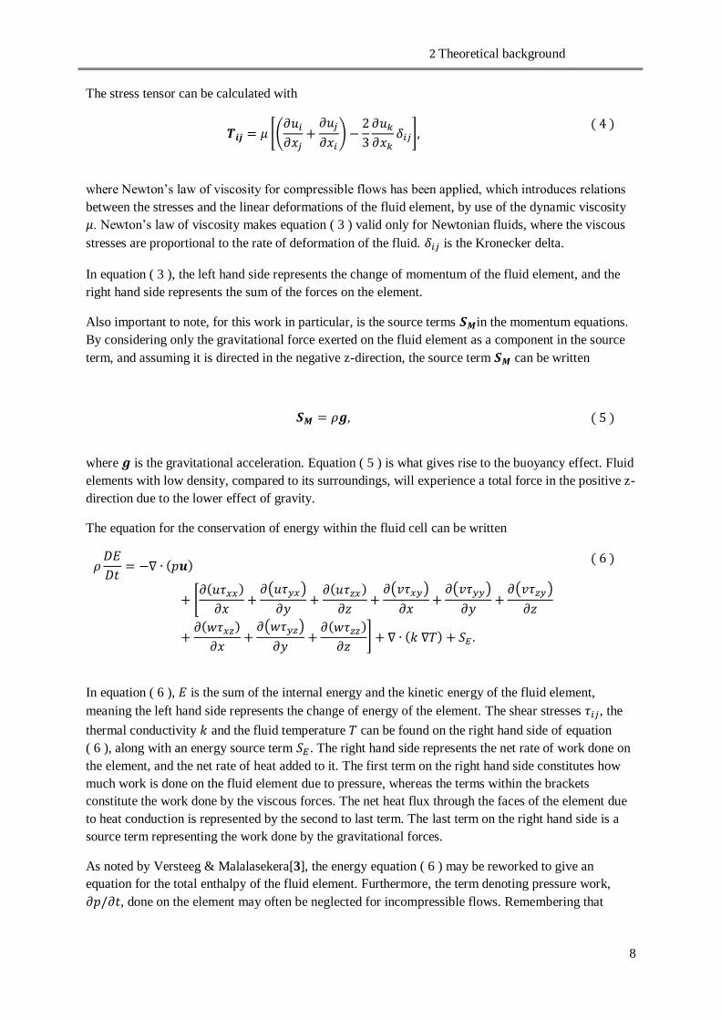
The stress tensor can be calculated with

( 4 )

where Newton’s law of viscosity for compressible flows has been applied, which introduces relations

between the stresses and the linear deformations of the fluid element, by use of the dynamic viscosity

. Newton’s law of viscosity makes equation ( 3 ) valid only for Newtonian fluids, where the viscous

stresses are proportional to the rate of deformation of the fluid. is the Kronecker delta.

In equation ( 3 ), the left hand side represents the change of momentum of the fluid element, and the

right hand side represents the sum of the forces on the element.

Also important to note, for this work in particular, is the source terms in the momentum equations.

By considering only the gravitational force exerted on the fluid element as a component in the source

term, and assuming it is directed in the negative z-direction, the source term can be written

( 5 )

where is the gravitational acceleration. Equation ( 5 ) is what gives rise to the buoyancy effect. Fluid

elements with low density, compared to its surroundings, will experience a total force in the positive z-

direction due to the lower effect of gravity.

The equation for the conservation of energy within the fluid cell can be written

( 6 )

In equation ( 6 ), is the sum of the internal energy and the kinetic energy of the fluid element,

meaning the left hand side represents the change of energy of the element. The shear stresses , the

thermal conductivity and the fluid temperature can be found on the right hand side of equation

( 6 ), along with an energy source term . The right hand side represents the net rate of work done on

the element, and the net rate of heat added to it. The first term on the right hand side constitutes how

much work is done on the fluid element due to pressure, whereas the terms within the brackets

constitute the work done by the viscous forces. The net heat flux through the faces of the element due

to heat conduction is represented by the second to last term. The last term on the right hand side is a

source term representing the work done by the gravitational forces.

As noted by Versteeg & Malalasekera[3], the energy equation ( 6 ) may be reworked to give an

equation for the total enthalpy of the fluid element. Furthermore, the term denoting pressure work,

, done on the element may often be neglected for incompressible flows. Remembering that


9

water is the fluid investigated in this work, and that it is considered incompressible, the pressure work

term can be ignored.

Similar to the equation used in Flores et al. [4], the simplified total enthalpy equation then takes the

form

( 7 )

where is the specific total enthalpy of the fluid cell, is the molecular thermal diffusivity, and is

a new source term.

2.2 Turbulence

2.2.1 General description of turbulence

The issue of turbulence in modern industry is a tough one, to say the least. On one hand, the equations

describing the nature of all fluid flows are clearly stated and ready to be implemented on all problems.

On the other hand, extremely few flow situations can be solved this way even with today’s super

computers of the year 2014, and most of these flow problems are not of industrial interest. Turbulence

is the main reason behind the large amount of computational power required to solve the equations

numerically.

Turbulence is a strictly three-dimensional phenomenon and the nature of turbulence can best be

described as chaotic, with its properties not yet fully understood. At low flow speeds, conditions

remain steady and this is referred to as laminar flow. With increasing flow speed however, the velocity

starts to fluctuate in a chaotic manner and the flow is referred to as turbulent. A useful measure of

exactly how turbulent the flow is, is a non-dimensional parameter named the Reynolds number . It

is defined as the ratio between inertia forces and viscous forces,

( 8 )

where is the characteristic velocity scale and is the characteristic length scale of the flow. is the

kinematic viscosity of the fluid, .

At low Reynolds numbers, flows remain steady (laminar), and at high they become unsteady

(turbulent). The transition between laminar and turbulent flow occurs at a critical Reynolds number,

although the magnitude of this number and the point in space where the transition takes place is

difficult to predict as they depend on a lot of variables in the specific case.

The reasons for the fluctuations in flow speed can be accounted to the chaotic behavior of turbulent

motions. Eddies are always present in turbulent flow fields and they present themselves as rotating

flows within a localized region. The length scales of the eddies can be as large as the characteristic

length scale of the flow field, and small enough for the eddies kinetic energy to be dissipated into heat

by means of molecular viscosity. The largest eddies contain the most energy, which they obtain from

the mean flow. Being that they are unstable they tend to break up, leaving behind smaller eddies. This

process carries on with the larger eddies transferring their energy to the smaller ones continuously.

This idea is called the energy cascade and was introduced by Richardson[5]. Figure 5 shows a

principle diagram of the energy cascade and how the large eddies transfer energy to the smaller ones.


10

It shows the how the energy of an eddy is dependent on the wavenumber of the eddy. Region I is

where the larger, energy-containing eddies form, and region III is where the small eddies dissipate.

The inertial subrange, region II, is where the larger eddies break up and transfer their energy to

successively smaller eddies.

Figure 5: A principle diagram of the energy cascade, showing how the energy spectrum function depends on the

wavenumber of the eddies.

It should be noted that turbulence is a flow property, and not a property of the fluid, and it is unique

for every flow condition. However, it is argued that the smallest scales of turbulence, known as the

Kolmogorov microscales, are universal and behave the same way for all turbulent flows at higher

Reynolds numbers (Versteeg & Malalasekera[3]).

2.2.2 LES turbulence model

Considering the fact that the large eddies contained in a turbulent flow field are highly dependent on

the mean flow and the geometrical features of the fluid domain, and that the small eddies are more of a

universal nature, one may come to the conclusion that interest lies in calculating the dynamics of the

larger eddies, and simply applying a model to capture the behavior of the smaller eddies. This is the

underlying thought of the LES turbulence modelling approach.

Using the LES method in this project was a given from the start. It was of interest to investigate the

possibilities of the LES method and to see what results it could give.

The key to separating the larger eddies from the smaller ones is to use a spatial filter. The filter should

be designed to accurately pick out the smaller scales and leave the larger scales intact. The general

definition of the filtering operation is as follows:

( 9 )


11

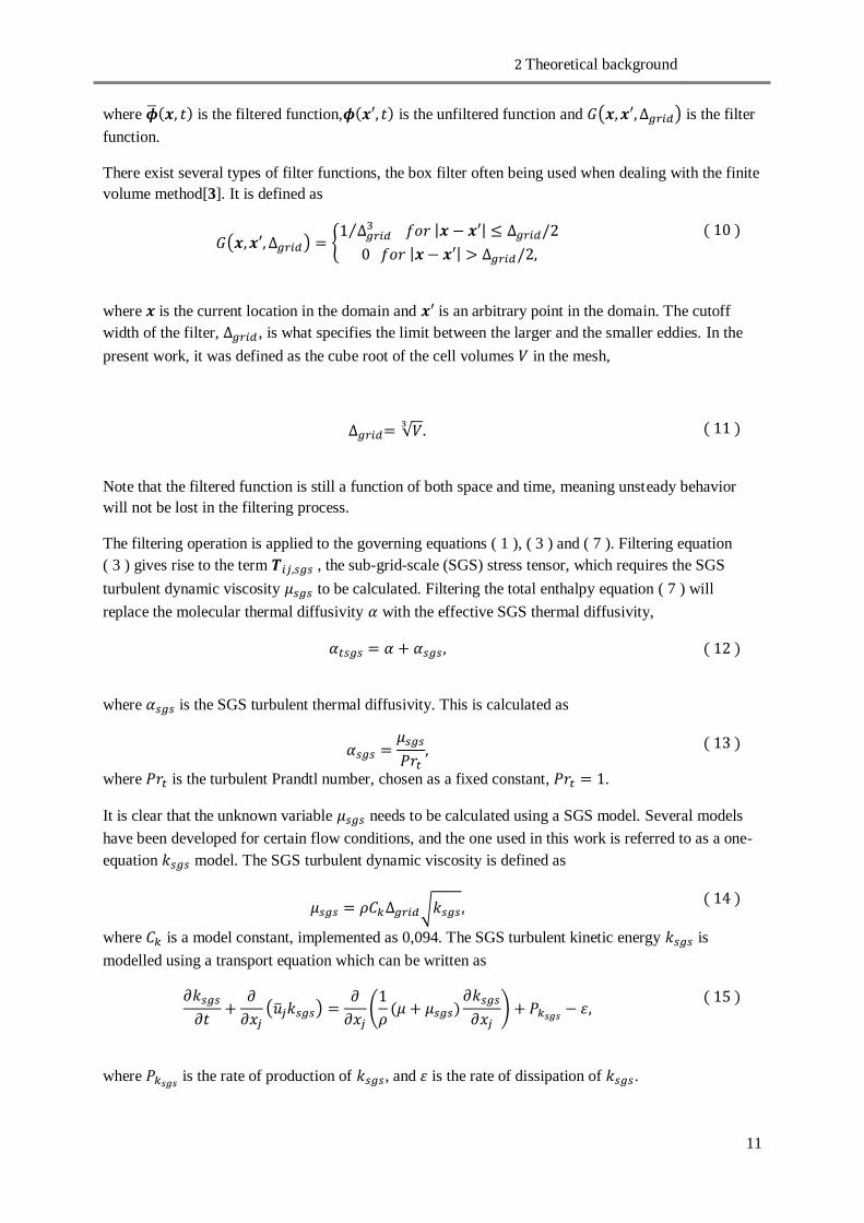
where is the filtered function, is the unfiltered function and is the filter

function.

There exist several types of filter functions, the box filter often being used when dealing with the finite

volume method[3]. It is defined as

( 10 )

where is the current location in the domain and is an arbitrary point in the domain. The cutoff

width of the filter, , is what specifies the limit between the larger and the smaller eddies. In the

present work, it was defined as the cube root of the cell volumes in the mesh,

( 11 )

Note that the filtered function is still a function of both space and time, meaning unsteady behavior

will not be lost in the filtering process.

The filtering operation is applied to the governing equations ( 1 ), ( 3 ) and ( 7 ). Filtering equation

( 3 ) gives rise to the term , the sub-grid-scale (SGS) stress tensor, which requires the SGS

turbulent dynamic viscosity to be calculated. Filtering the total enthalpy equation ( 7 ) will

replace the molecular thermal diffusivity with the effective SGS thermal diffusivity,

( 12 )

where is the SGS turbulent thermal diffusivity. This is calculated as

( 13 )

where is the turbulent Prandtl number, chosen as a fixed constant, .

It is clear that the unknown variable needs to be calculated using a SGS model. Several models

have been developed for certain flow conditions, and the one used in this work is referred to as a one-

equation model. The SGS turbulent dynamic viscosity is defined as

( 14 )

where is a model constant, implemented as 0,094. The SGS turbulent kinetic energy is

modelled using a transport equation which can be written as

( 15 )

where is the rate of production of , and is the rate of dissipation of .


12

Closing this system of equations is done with

( 16 )

( 17 )

where is another model constant, implemented as 1,048. The filtered rate of strain tensor is

calculated with

( 18 )

where is the filtered velocity field.

2.2.3 Near-wall resolution concerns

The LES approach of modelling turbulence is still costly and rarely used in the industry. This is

mainly due to the mesh requirements. Pope[6] notes the distinctions between the different variants of

LES. He notes that LES should resolve most of the turbulent scales in the bulk flow region, and

capture at least 80% of the turbulent kinetic energy here. Failing to do so qualifies the simulation as

VLES (Very Large Eddy Simulation). Depending on whether or not the wall boundary layer is

properly resolved, the simulation can be classified as LES-NWR (LES-Near-Wall-Resolution) or LES-

NWM (LES-Near-Wall-Modelling), and further noting that the mesh required to do LES-NWR causes

the simulation to be extremely costly for high Reynolds number flows. Estimating the amount of

turbulent kinetic energy resolved, compared to the total in the system, is a good way of perceiving if

the mesh is sufficiently fine, although it will not be done in this work.

The LES-NWM often implies the use of so called wall functions, which are designed to model the

effects the wall boundaries have on the flow field. Using a function to model the flow near the wall

will remove the need to resolve the near-wall region with a fine mesh. This of course has a large effect

on the overall simulation cost, and can make an expensive LES simulation comparably cheap.

However, there are some major drawbacks with the usage of these wall functions. Ferziger & Perić[7]

bring up the issues with the models when the flow is not bounded to a wall. For the wall functions to

work properly, the computational mesh needs to have a node at a position close to the wall. The

dimensionless distance y+ measured from the wall is defined as

( 19 )

where is the shear velocity and y is the distance from the wall. From equation ( 19 ) we see that by

placing a node at different distances from the wall, we can effectively control the y+ value. Ferziger &

Perić note that for certain wall functions, the node closest to the wall must be placed such that


13

, otherwise the wall functions will give erroneous results. In separated flow regions, this is of

course very hard to satisfy especially if the flow is unsteady. Different wall functions can be used in

different zones of the wall boundary, but estimating where the flow is attached and where it is

separated is a tedious task. The practical option is to simply use a consistent wall function throughout

the domain, or to use none at all.

2.3 Dimensionless numbers

2.3.1 The Rayleigh number

Along with the Reynolds number ( 8 ) and the y+ number ( 19 ), there exists a large number of

dimensionless numbers which could be useful to study within a fluid flow problem.

The Rayleigh number is one of them, which according to Bergman et al. [8] can give a good

representation of the transition between a laminar boundary layer, and a fully turbulent boundary

layer. The Rayleigh number can be defined as the product between two other dimensionless

numbers, namely the Grashof number and the Prandtl number :

( 20 )

A commonly studied buoyancy driven flow problem is a hot vertical flat plate surrounded by colder

fluid. The hot plate will heat up the fluid close to it and, due to buoyancy forces, cause it to rise

upwards. For the hot plate fluid flow problem, the Rayleigh number is calculated with ([9] )

( 21 )

where is the volume coefficient of expansion, is the density difference between the fluid

far away from the wall and the fluid near the wall, and is the temperature difference

between the fluid near the wall and the fluid far away from the wall. Furthermore, is the distance

from the leading edge of the plate and , , and are all taken to be average values of the

kinematic viscosity, the dynamic viscosity, the specific heat capacity and the thermal conductivity

respectively, for the fluid.

Bergman et al. suggests the critical Rayleigh number for when the boundary layer starts to become

turbulent is above in the case of the hot vertical flat plate, and Holman [9] claims the transition

can begin at values of . Although the hot plate fluid flow problem is very different from the one

studied in this work, equation ( 20 ) can still give a rough hint of how crucial it is to have a properly

resolved boundary layer. Having turbulence very close to a solid boundary puts greater requirements

on the mesh than if the boundary layer is mainly laminar. and has been chosen as the temperature

and density of the warm fluid in this problem (555K and 747 kg/m3), whereas and is chosen as

the properties of the cold fluid (288K and 1002 kg/m3). , the distance from the leading edge of the

plate in equation ( 20 ), has been chosen as the approximate distance between the mouth of the pipe

and the 90° bend inside the pipe insert.


14

2.3.2 The Courant number

The Courant number is of interest to study when it comes to numerical stability and accuracy.

Certain differential schemes used in CFD analyses will not function properly and may give poor

results, if the Courant number is too high. A general consensus is that if values of the Courant number

exceed 1, the numerical stability and accuracy may be compromised. The Courant number depends on

the fluid velocity, the time step size and the computational cell size, and can be calculated in each

computational cell as

( 22 )

where is the velocity in a Cartesian direction, is the time step size and , and are the

lengths of the computational cell in the Cartesian directions.

3 Method

15

3 Method For this work, the CFD method was chosen to be used as the analysis tool for the flow problem

studied. The CFD method has its roots in a number of equations governing fluid flow and can describe

a large number of flow problems. The equations used in this work are presented in the previous

chapter. By creating a computational domain, dividing it into a finite number of smaller volumes and

then solving these conservation equations in each volume, we can basically simulate any type of flow

condition if the right equations are used. The computational domain would of course have to represent

the geometry well, and the conditions set at the boundaries of the domain also have to be realistic for

the flow case. These are the basics of the CFD method. CFD is unfortunately expensive when

compared to simpler fluid flow analysis methods and is therefore not always used in industrial projects

such as this one. Despite this, the method of conducting a CFD analysis of this particular fluid flow

problem was chosen in order to show the possible strengths and shortcomings of the CFD approach.

There are many mistakes which can be made in the preparation work for a CFD calculation, and every

simplification in the model needs to be done with caution. In the following sections of this chapter, the

creation of the computational model is described along with a description of how the simulations were

run.

3.1 Model simplifications A simplified model of the cooling system and the surrounding regions was created for the calculations.

The four pipe inserts are spaced with around 110D, where D is the diameter of the mouth of the pipe.

They were considered to be far away from each other, so only one of the four pipe systems was used

in the model. The suspension system which carries the pipe insert on the reactor pressure vessel wall

was not included in the model, also because it was seen as far away from the mouth of the pipe, with a

distance of 3D. Also not included in the model is the wall of the vessel and the components in front of

the pipe insert, such as the reactor core shroud, which are placed about 7D from the pipe. The thermal

insulation depicted in figure 3 has also not been included in the computational domain. The reason for

this is also to simplify the meshing process and to prevent complications that could arise when trying

to simulate flow through this complex structure.

General geometrical modifications to the pipe, such as the removal of the hole in the lifting eye on top

of the pipe insert, have been made to save further time in the project. The lifting eye structure was

however kept on the pipe insert, as it was thought to cause disturbances in the flow which could affect

how the flow field would behave just below, and inside the pipe. Shown in figure 6-8 is the simplified

computational domain used. It also shows how the pipe structure outside of the vessel was modelled,

where a bend and a downward slope can be noted about 3 m from of the vessel wall. There would be

more bends and the previously mentioned gate valve further down the pipe, although these parts are

not included in the model since they are in fact far away from the reactor. It was assumed that the

warm water would not reach these regions for a very long time, and would probably slow its

movement out of the reactor vessel when it reaches the first pipe bend. Considering the fact that the

pipe after this bend has a 14° downward slope, the warm water should not be able to move down past

the bend due to the buoyancy forces. Heat could still be transported further down into the pipe by

means of convection, conduction and radiation, although it would probably be done at a fairly slow

pace. The pipe in the computational domain was therefore not extended far beyond this downward

pipe bend.

3 Method

16

The size of the computational region representing the inside of the reactor pressure vessel, more

specifically the downcomer, was made sufficiently large enough to capture the flow field of interest.

The flow field of interest would be the jet forming below the pipe insert, during the pump driven stage

of the simulation, and the flow of warm water into the mouth of the pipe, during the buoyancy driven

stage. Trial and error was a method employed to get a good size of the downcomer domain. By

creating an arbitrarily sized domain and studying the results from it, it was possible to determine just

about how small the domain could be kept and still produce reasonable results.

Figure 6: The simplified geometry of the pipe insert used in the simulation.

Figure 7: The simplified geometry used in the simulation.

3 Method

17

Figure 8: The simplified geometry used in the simulation and the placement of the computational domain, compared to the placement of actual components surrounding the downcomer.

Further simplifications in the model include ignoring the effects heat transfer due to radiation. This

was done to simplify the simulation process and not introducing further unknowns in the form of a

radiation model. Heat transfer from the fluid region to the solid region, such as the pipe and the pipe

insert, was also ignored. Capturing the correct heat flux into the pipe would require the solid geometry

to be correctly modelled, and remembering that parts such as the thermal insulation shown in figure 3

was left out of the model, the heat transfer to the surroundings would be quite inaccurate in these

regions compared to the real case.

3.2 Computational mesh Before a computational mesh is created, one must consider the possible flow field in the domain and

try to estimate where a finer mesh is needed. For the problem at hand, this is a complicated task

because two very different flows will be simulated on the same mesh. First, the cooling system will

transport the cold water into the reactor vessel. After that, the cold water will stop flowing and

buoyancy forces will drive the warm water up into the pipe. These are two very different scenarios and

they would both gain from having a unique computational mesh created for each case. The actual

domain could also be changed if one would only consider one of these flows, such as having a smaller

downcomer region for the buoyancy driven flow, or a shorter pipe region for the pump driven flow.

However, since the buoyancy driven flow case is of major interest for this project it was decided that

the computational mesh should be generated with this case in mind and be used for both flow

scenarios. The simulation of the pump driven flow would of course not be optimum with regards to

time and results, but by only creating one mesh rather than two the time consumption for the project

could be kept reasonable.

When considering the possible flow field for the buoyancy driven flow, one can imagine that chaotic

flow structures would form near the mouth of the pipe, where the warm water enters and the cold

water exits. The difference in temperature would be high, especially in the beginning of this flow

scenario when the water in the pipe has not yet started to increase in temperature, and a chaotic mixing

should occur between the warm and cold water. Further into the simulation, it can be imagined that

distinct layers would be seen inside the pipe, with a layer of warm water on top of a layer of cold

water, and a mixing layer in between the two. It should therefore be noted that a well resolved

boundary layer near the walls of the pipe may not be sufficient for capturing the flow physics at hand.

A fine grid concentration is also necessary in the centre of the pipe where the mixing of warm and

3 Method

18

cold water occurs. Since the position of this mixing layer will change over time, a fairly uniform

distribution of cells was used, as shown in figure 9.

Figure 9: The principle mesh structure in a cross section of the pipe.

The downcomer region should also be properly resolved with considerations to the potential flow field

of the buoyancy driven flow. A downward flow in the downcomer is always present and will most

likely be highly disturbed as it passes the pipe insert. The mesh should therefore be refined around and

immediately below the pipe insert to capture this unsteady flow.

The software pre-processing tool ANSA was used for mesh generation in this work. The methods of

meshing with this tool involve creating surface meshes on boundaries of the domain and extruding

these to form the volume mesh. The extrusion of the surface meshes can be done in an ordered

fashion, which creates a properly structured volume mesh, although this method can however not be

used on all geometries as it puts certain requirements on the surface meshes connected to the volume

mesh. Employing ordered meshes can decrease the amount of cells in a mesh, and make it easier to

control the quality of the mesh. However, if the geometry is too complex, a less ordered mesh

generation must take place. This creates a mesh with a more unstructured appearance.

The ANSA meshes were generated using both methods. The inside of the pipe was created with an

ordered mesh of hexahedral cells. The cross section shown in figure 9 is consistent through the entire

pipe. An ordered mesh of hexahedral and pentahedral cells was made just above the mouth of the pipe,

and down to the bottom of the domain. The rest of the domain, which is around the pipe insert and

above it, was given an unordered mesh with tetrahedral and pyramid cells. Creating an ordered mesh

in this region proved to be difficult and would require a lot more time. It was found that the main

complication with using the ordered meshing method in this region was the lifting eye attached to the

pipe insert. Had this been left out of the model, the ordered method could have been used fairly easily.

The region above the pipe insert and near the inlet was kept fairly coarse since the flow here was

expected to be quite steady.

For the purpose of investigating how the results would be affected by simulating using a coarse or a

fine mesh, several meshes were generated. They all had the same basic structure described above, but

differed greatly when it came to the size of the cells in all regions.

In the interest of saving time when it comes to the mesh generation process, another method of

creating a computational mesh was investigated. The utility snappyHexMesh[10] implemented in

OpenFOAM 2.3.x has the ability of automatically creating 3D meshes from well-defined geometries.

It does require some user input, but is essentially a far quicker way of generating a high quality

computational mesh, especially for a complex geometry. The basic process of generating the meshes

can be described as follows:

3 Method

19

1. A base mesh is created without regard to the geometry boundaries.

2. The base mesh is refined by splitting the cells at the geometry boundaries.

3. The cells located outside of the domain boundaries are removed.

4. The vertices of the cells adjacent to the geometry boundaries are snapped to the geometry to

form smooth mesh boundaries.

Further options include refining the mesh in the boundary layer region, although this was not utilized

in the present work. It can be argued that it is more difficult to control the placement of the cells with

the snappyHexMesh utility, since it is text based with no graphical user interface. The mesh

constructed with the utility for this work was not optimal in this respect. More time could be spent on

carefully refining the mesh in regions of interest, but due to time constraints a faster approach was

used. It should be remembered that the geometry used in CFD simulations often needs to be somewhat

modified before the mesh can be generated, by removing small details and smoothing surfaces. These

modifications will still have to be made for the snappyHexMesh utility and could potentially be far

more time consuming than the actual mesh generation process, meaning the snappyHexMesh utility

would not save much time for the user.

In total, four meshes were used in the simulations and the size difference can in one way be quantified

by looking at the number of cells in the mouth of the pipe. Shown in figure 10 are the pipe openings

and the cell distribution for each mesh. It shows that the coarsest ANSA mesh only had 14 cells across

the diameter of the pipe, whereas the finest ANSA mesh had 44 cells. The finest mesh was also the

only one to have a notably different size distribution of cells, with thinner cells near the boundaries.

The mesh generated by snappyHexMesh had only 12 cells across the diameter of mouth of the pipe. It

should be noted that the number of cells in the diameter of the pipe increases as the diameter increases

for the snappyHexMesh grid, but stay the same for the ANSA grid.

3 Method

20

Figure 10: The cell distribution in the mouth of the pipe for the four different meshes investigated. Cells marked grey are surface cells and cells marked blue are volume cells.

Table 1 presents the meshes used in the present work.

Table 1: Cell-count for each mesh.

Mesh name Cells in the diameter of the pipe opening Total number of cells

Coarse (ANSA) 14 0,14M

Medium (ANSA) 28 1,5M

Fine (ANSA) 44 3,2M

Snappy (snappyHexMesh) 12 1,8M

In figure 11, the medium sized ANSA mesh is presented from different views. As mentioned earlier,

the coarser and finer ANSA meshes are similar in design, only with differently sized cells. Figure 12

displays the snappy mesh from different views.

3 Method

21

Figure 11: The medium ANSA mesh of the domain, shown in different cross sections around the pipe insert. Note the ordered mesh region below the mouth of the pipe, and the unordered region above.

3 Method

22

Figure 12: The snappy mesh generated by the snappyHexMesh utility, shown in different cross sections around the pipe insert.

3.2.1 Mesh quality

It is important to have cells of good quality in a computational mesh, otherwise problems with stability

and convergence of the simulation could arise. The two larger ANSA meshes were designed with

quality in mind and the skewness and orthogonality of the cells, as well as the smoothness of the mesh

was checked. The snappyHexMesh utility generally creates cells of very good quality, but this mesh

was also thoroughly checked in order to quantify any issues present.

Exactly how the skewness quantity is defined in OpenFOAM will not be explained in this work but it

can generally be said that it is a measure of how skewed the cell faces are in a computational mesh. A

low value for the skewness indicates good cell quality. An implemented utility in OpenFOAM called

checkMesh is used to check the validity of the computational mesh used in a simulation. If the utility

fails to confirm the mesh to be of good quality, stability issues are prone to occur during the

simulation. The utility fails if the maximum face skewness value of any cell face in the mesh is above

the value 4. All of the meshes investigated in this work passed the checkMesh test.

For the ANSA-generated meshes, the ordered cells within the pipe and below the pipe insert showed

excellent quality with regards to skewness, whereas the unordered cells above the pipe insert were of

somewhat lower quality. The snappy mesh showed excellent skewness qualities throughout the

domain. The cells of highest skewness in the snappy mesh were found along curved boundaries where

3 Method

23

they have changed their configuration during the snapping stage of the meshing process to conform to

the geometrical features.

It is always good to employ several quality quantities when studying a mesh and orthogonality is

another measure of how good a cell shape is. It can be explained by studying figure 13. Considering

vectors from the centre of a cell to the middle of the cell faces, and checking the angle between these

vectors and the normal of the cell faces, one can estimate how good the cell shape is[11]. If the angle

between the vectors is small, a good orthogonality is present.

Figure 13: OpenFOAM's definition of non-orthogonality. The figure shows two 2D cells located in the same plane and the non-orthogonality of the common face between them.

The checkMesh utility views a value above 70° for the non-orthogonality as too high. The

orthogonality was overall good in both meshes, although the lowest quality was found in the pipe

region of the finest mesh (see figure 14). The cells along the boundary here are seen to have a lower

orthogonality, although still within tolerable limits. Again, no major quality concerns were found with

the snappy mesh.

Figure 14: Cells in the pipe region of the fine ANSA mesh, colored by values of non-orthogonality.

Smoothness, also called growth ratio, is a measure of how the volumes of two adjacent cells differ. A

fairly small growth ratio was achieved in practically all regions of the ANSA meshes. Large growth

3 Method

24

ratios are unwanted and the largest was found in the transition region between the ordered and

unordered meshes, where the volume of a hexahedron could be up to nine times as large as its adjacent

pyramid cell, as shown in figure 15. The transition region was therefore deliberately placed at a

distance from the mouth of the pipe to minimize the effect of this poor smoothness (see figure 11).

Figure 15: Cells around the transition region from ordered to unordered grid of the fine ANSA mesh, colored by the smoothness factor.

The snappyHexMesh utility refines by essentially splitting larger cells into smaller ones. One

hexahedral cell is always split into eight smaller hexahedral cells of similar size. This means there will

be some issues when it comes to smoothness in the mesh. As seen in figure 12, the transition regions

between larger and smaller cells was always kept far away from the pipe insert boundaries but is

essentially impossible to rid of completely without having a uniform refinement over the entire

domain. The largest smoothness discrepancy was seen in the pipe region, where such a transition is

placed.

The overall quality of the three larger meshes was considered good. The quality of the coarsest mesh

however was not of major concern as it was only generated to give an extreme example of how the

problem could be meshed and perhaps even solved. This mesh was however checked using the

checkMesh utility in OpenFOAM to make sure no degenerate cells existed.

Mesh quality statistics are presented in table 2.

3 Method

25

Table 2: Mesh quality statistics.

Coarse Medium Fine Snappy

Percentage of cell-faces with skewness < 0,2 93,3 92,2 96,9 99,8

Max skewness of cell-faces 2,54 1,08 1,23 2,75

Percentage of cells with non-orthogonality < 40 92,5 99,9 94,8 99,99

Max non-orthogonality of cells 74,0 60,4 56,5 52,9

Max aspect ratio of cells 15,8 30,9 68,8 5,36

3.3 Initial and boundary conditions It is of critical importance that the boundary conditions in a fluid flow problem are well posed and

physically correct. Badly posed boundary conditions can cause faulty results or rapid divergence of the

calculations, as noted by Versteg & Malalasekera[3]. Choosing the right conditions for each boundary

could be a matter of trial and error. It is not always clear which boundary condition will produce the

most stable and correct solution, and in some cases when the computational domain is badly made, it

may not be possible to set a correct boundary condition. The OpenFOAM software requires the user to

specify boundary conditions for all quantities used in the simulation on all boundaries. All conditions

are presented in table 5 in the appendix and certain selected conditions are described in greater detail

below.

3.3.1 Inlet and outlet boundaries

This domain has two inlets and one outlet. The inlet of the pipe is the one that provides the flow of

cold water through the pipe and into the downcomer during the pump driven flow, and the downcomer

inlet simulates the downward flow in the reactor vessel. Both inlets were chosen as uniform velocity

inlets. The pipe inlet could have been given a varying velocity profile, but it was assumed that the

profile would evolve by itself further downstream the pipe since the pipe is long. The downcomer inlet

had a constant velocity of 0,468 m/s, uniform across the whole face, and the pipe inlet had a uniform

constant velocity of 2,708 m/s during the pump driven flow. The transition between the pump driven

flow and the buoyancy driven flow took place during one second, meaning the pipe inlet velocity was

linearly decreased to 0 m/s over the course of a second, as shown in figure 16. The downcomer

velocity was kept the same. The outlet boundary, which is positioned at the bottom of the downcomer

region, kept a zero gradient velocity condition.

Figure 16: Pipe inlet velocity as a function of time, showing the linear transition from pump driven flow to buoyancy driven flow.

Both inlet boundaries were given zero pressure gradient conditions, whereas the outlet boundary had a

uniform constant pressure of 0 Pa across the whole face. Absolute values of the pressures in the

domain are never used when solving the discretized equations for the problem, but rather pressure

differences and since the thermophysical properties of the simulated water are set to vary with

temperature, and not pressure, it is possible to set a 0 Pa pressure on the outlet even though the

3 Method

26

operating pressure of the reactor vessel is around 7 MPa. This could not have been done had the

simulation utilized an equation of state operating like for example the ideal gas law, which requires an

absolute pressure to calculate certain fluid properties.

The temperature of the pipe inlet boundary was set as 288K, and the downcomer inlet temperature was

555K. The temperature of the pipe inlet can be higher than 288K if the pool from which the water is

pumped has insufficient cooling, although in the interest of simulating the worst case scenario for the

pipe system, having a large temperature difference between the cold water and the warm water is

desirable.

The downcomer outlet was given a temperature boundary condition specified as inletOutlet in

OpenFOAM. This means it is possible to specify the temperature of the fluid coming into the domain

when backflow occurs. A temperature of 555K was chosen as the inlet value on the boundary, since

this was the expected temperature in the downcomer region during the buoyancy driven flow. When

the boundary is working like an outlet, a zero gradient condition was used.

3.3.2 Symmetry boundaries

All four sides of the downcomer region inside the reactor vessel were given symmetry boundary

conditions. Whether or not this is proper usage of the symmetry condition is debatable, although it is

clear that in this particular flow case, the further away the symmetry boundary is placed from the

region of interest, which is the mouth of the pipe, the less it will impact the results. With this in mind,

a brief investigation was made in which the symmetry boundary of the domain closest to where the

pressure vessel side would be located (see purple boundary in figure 17) was changed from a

symmetry boundary condition to a no-slip wall condition (see table 5 in the appendix). The medium

sized mesh was used for the investigation.

3.3.3 Wall boundaries

The inside of the pipe and the outside of the pipe insert were seen as no-slip walls with zero pressure

gradients and a constant velocity of 0m/s in all directions on the faces. No wall functions were used on

any wall boundaries in the domain. Furthermore, all walls in the domain were considered to be

adiabatic, meaning they had zero gradient temperature conditions.

The boundaries of the domain are shown in figure 17.

Figure 17: Boundaries of the computational domain.

3 Method

27

3.3.4 Initial conditions

Providing the solver with a good initial field can greatly reduce the computational costs and give better

convergence for the first time steps of the simulation. In some cases, a good initial guess is required

for the solution to converge at all. In this work, it was decided that a simple initialization would be

used. It was mainly important to quickly form the correct temperature field inside the pipe during the

pump driven stage of the simulation, and also to develop realistic velocity profiles. Therefore a steady

state simulation was done on the domain with the above described boundary conditions and without

the use of a turbulence model. A good convergence was seen and the initialization process was quick.

3.4 Fluid properties Using a correct fluid model is essential for a simulation to be accurate. The fluid in the domain ranges

in temperature between 288K and 555K which means some properties, which are temperature

dependent, will differ greatly within the domain. The fluid model needs to capture these properties of

water pressurized at 7 MPa in a realistic way. Using steam table calculators based on the work of

IAWPS[12] the density , specific heat capacity , thermal conductivity and dynamic viscosity

of the fluid was produced in tables. Unfortunately, it is not possible to import tables of data to

represent the fluid properties into the solver used for the simulations. Instead, these properties were

estimated using polynomials to match curves of the exact data. In figure 18, the polynomial curves are

plotted against the exact data. The polynomials used are presented in table 6 in the appendix.

3 Method

28

Figure 18: The polynomial curves used to estimate the fluid properties , , and , plotted against true property data. The

grey regions mark the temperature operating range for the simulations.

These polynomials used are all of degree five, which may seem high but any lower degree of the

polynomials would result in inaccurate predictions and could affect the results negatively.

3.5 Numerical solution properties The simulations were all carried out using the open source CFD code OpenFOAM 2.3.x. It uses the

finite volume method for solving partial differential equations and has the ability to solve a wide range

of fluid flow problems with the pre-programmed solver applications. The OpenFOAM software has

previously been used at Forsmarks Kraftgrupp AB in other LES analyses ([13]) and it was therefore of

interest for the company to further strengthen their insight in the software. The pre-programmed solver

used in this work was called buoyantPimpleFoam and is mainly designed to simulate transient

compressible fluid flows with heat transfer. The fluid in the current work is water, which is considered

to be an incompressible fluid, so the use of compressible governing equations could be seen as ill

fitted. However, using a solver designed for incompressible flows often implies ignoring the term

in equation ( 1 ), which is obviously not correct in the current flow problem. The system of

equations used in the buoyantPimpleFoam solver is closed using the above mentioned polynomials,

similar to how an equation of state is used.

3 Method

29

3.5.1 Parallel processing

Parallel processing was utilized for all simulations conducted. Performing simulations using the LES

method of modelling turbulence is known to be costly and if proper resolution in both time and space

is wanted, serious computing power is required. The simulations were carried out on a computer

cluster where between 32 and 112 cores were utilized for each simulation, depending on which mesh

was used. The project was aimed to be completed from start to finish in about 6 months. This time

constraint, along with the size of the computer cluster, put a limit on just how thorough well resolved

the LES could be.

It is not always preferable to use as many cores as possible during a simulation, due to the fact that

communication between the cores takes time. Solving a problem on a single core requires no

communication between cores, but instead forces the single core to solve large matrices by itself.

Using parallel processing, the matrices can be divided into smaller ones and dispersed amongst the

cores. Quite simply, a balance needs to be found between reducing the size of the matrices each core

has to solve, and reducing the time consumption of communications between the cores. Trial and error

is the simplest way of finding out just how many cores will produce the fastest result for the current

problem.

An interesting note to make on the topic of computational speed and the solution of these matrices is

how a multigrid approach can effectively decrease the time it takes to solve them. The multigrid

technique can be described as discretizing the system of equations on a mesh much coarser than the

one provided for the solver. After the discretized equations are solved, the solver refines the mesh and

repeats until it finally solves the problem on the specified mesh. This method has proved to increase

convergence speed and is often utilized in CFD codes[3]. However, considering the above discussion

about finding a balance between solving matrices on each separate core and reducing communications,

it is easy to conclude that the first stages of this multigrid technique do not require a large amount of

parallel cores. A method of letting only a small number of cores solve the problem on the coarsened

meshes is implemented in OpenFOAM 2.3.x and was used in this work.

3.5.2 PISO iterative solution procedure

Solving the equations described in chapter 2 was done using an iterative procedure. The equations

have to be discretized, and this is carried out using the computational mesh generated for the problem.

There are several methods for coupling the set of equations to each other, one of which will briefly be

described below.

The PISO (Pressure Implicit with Splitting of Operators) algorithm is a way to couple the velocity

with the pressure in the domain. It was developed by Issa[14] and has its basis in the SIMPLE

algorithm which was developed previously by Patankar & Spalding[15]. The PISO method

implemented in OpenFOAM can be described as follows:

1. The pressure field for the current time step is guessed, often by setting it equal to the previous

time step.

2. The momentum equations, discretized in each cell of the mesh, are solved to obtain the

velocity field.

3. The discretized energy equation is solved.

4. The pressure field is corrected using the obtained velocity field to satisfy continuity.

5. The velocity field is corrected using the newly corrected pressure field.

After this, the PISO algorithm repeats step 4 and 5 simply by correcting the pressure field yet again,

and updating the velocity field for the second time, with the newly corrected pressure field. In

3 Method

30

OpenFOAM, it is possible to set the amount of correcting loops. In the current work, a total of 3

correcting procedures were used to ensure good convergence. Another option is to add a secondary

pressure correction in each correcting loop to further enhance the convergence and make up for the use

of a non-orthogonal mesh. This secondary correction was used since all cells in the computational

meshes were not completely orthogonal. After all specified pressure correctors are done and the

velocity field is updated, the transport equations for other quantities, such as the turbulent quantities,

are solved and the PISO loop finishes.

It is possible to solve the problem using the SIMPLE algorithm, which does not repeat step 4 and 5 as

the PISO algorithm does, but rather checks for convergence. If convergence is not met, the SIMPLE

loop is repeated. For transient simulations, the PISO algorithm is stronger than the SIMPLE algorithm

due to the fact that it requires no additional iterations after it finishes the PISO loop. This also means

no relaxation factors should be used in the PISO loop. A sufficiently small time step is however

required to yield accurate results[16].

If the simulation shows unstable behavior, it is possible to repeat the PISO loop until better

convergence is met. This does of course increase the computational time, but could benefit certain

simulations. When using the coarse computational mesh in this work, it was found that stability was a

major issue possibly due to cells of low quality. By repeating the PISO loop several times until good

convergence was met in each time step, the issues were resolved. This method of repeating the PISO

algorithm is called the PIMPLE method in OpenFOAM, because it is done in the spirit of the SIMPLE

algorithm which does not finalize a time step until convergence is met. It is hard to motivate the use of

the PIMPLE algorithm for the larger meshes as additional PISO loops are costly, but computational

cost for the coarse mesh still managed to be kept low.

To further strengthen the use of the PISO algorithm, as opposed to the tougher convergence criteria of

the PIMPLE algorithm, a simulation was performed in which the PIMPLE algorithm was used on the

medium sized mesh. The PIMPLE algorithm was activated in the beginning of the buoyancy driven

stage of the simulation and it was found to do the PISO loop twice for each time step to achieve

convergence. The computational time did therefore almost double, compared to the original simulation

where only one PISO loop was used for each time step, and due to time constraints in the project, the

PIMPLE simulation was only run for about 100 seconds of the buoyancy driven stage.

3.5.3 Further simulation properties

It should be stressed that the first stage of the simulation, when cold water flows into the reactor, is

only done to give a good starting point for the second stage of the simulation, when buoyancy forces

carry the warm water into the pipe. The first stage is meant to create turbulent structures in the

domain, which the initialization had failed to do since it did not utilize a turbulence model. The

forming of the turbulent structures is a process which may take some time. It was estimated that the

time it takes for a particle to travel from the pipe inlet to the domain outlet was about 2 seconds and

three flow-throughs of a particle, about 6 seconds, were seen as a sufficient simulation time to form

the necessary realistic structures. The pipe inlet flow is decreased over the course of 1 second before

the buoyancy driven stage of the simulation begins. At time 0, the pipe inlet flow is completely

stopped. The lengths of the various simulations are presented in table 3.

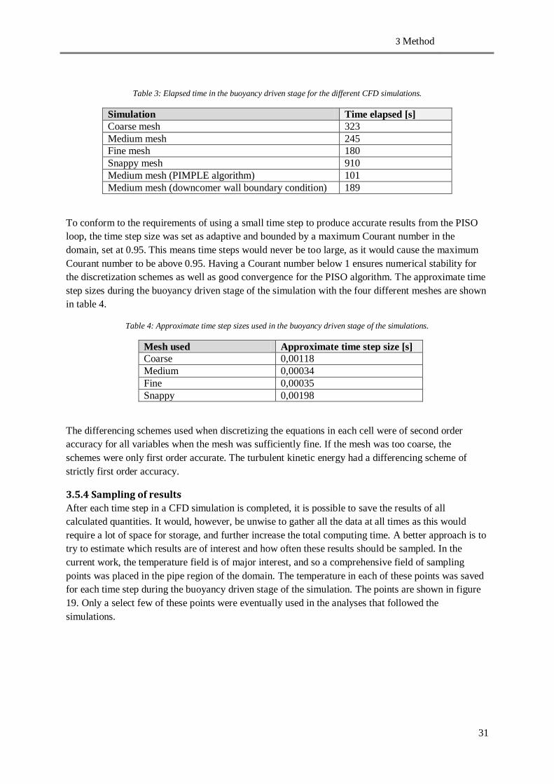
3 Method

31

Table 3: Elapsed time in the buoyancy driven stage for the different CFD simulations.

Simulation Time elapsed [s]

Coarse mesh 323

Medium mesh 245

Fine mesh 180

Snappy mesh 910

Medium mesh (PIMPLE algorithm) 101

Medium mesh (downcomer wall boundary condition) 189

To conform to the requirements of using a small time step to produce accurate results from the PISO

loop, the time step size was set as adaptive and bounded by a maximum Courant number in the

domain, set at 0.95. This means time steps would never be too large, as it would cause the maximum

Courant number to be above 0.95. Having a Courant number below 1 ensures numerical stability for

the discretization schemes as well as good convergence for the PISO algorithm. The approximate time

step sizes during the buoyancy driven stage of the simulation with the four different meshes are shown

in table 4.

Table 4: Approximate time step sizes used in the buoyancy driven stage of the simulations.

Mesh used Approximate time step size [s]

Coarse 0,00118

Medium 0,00034

Fine 0,00035

Snappy 0,00198

The differencing schemes used when discretizing the equations in each cell were of second order

accuracy for all variables when the mesh was sufficiently fine. If the mesh was too coarse, the

schemes were only first order accurate. The turbulent kinetic energy had a differencing scheme of

strictly first order accuracy.

3.5.4 Sampling of results

After each time step in a CFD simulation is completed, it is possible to save the results of all

calculated quantities. It would, however, be unwise to gather all the data at all times as this would

require a lot of space for storage, and further increase the total computing time. A better approach is to

try to estimate which results are of interest and how often these results should be sampled. In the

current work, the temperature field is of major interest, and so a comprehensive field of sampling

points was placed in the pipe region of the domain. The temperature in each of these points was saved

for each time step during the buoyancy driven stage of the simulation. The points are shown in figure

19. Only a select few of these points were eventually used in the analyses that followed the

simulations.

3 Method

32

Figure 19: Location of the points inside the pipe region where values of temperature were sampled during the simulation.

It is of course wise to save restart points at certain time levels, where all fields necessary for a restart

are saved. This was done every 3 seconds. In addition to this, the velocity and temperature fields of the

whole domain were saved about 5 times per second so that a good visualization of these fields could

be made in post-processing.

3.6 Relap5 software To provide a stronger analysis of the method chosen to solve the current fluid flow problem, it is

preferable to approach the problem with different methods. CFD analyses are costly, especially when

using scale-resolving simulations. A cheaper approach is to utilize a code which does not model

complex phenomena such as turbulence.

The Relap5 thermal-hydraulic code was created in 1979 and has been under development ever since. It

is developed by Idaho National Laboratory and is designed to analyze the thermal-hydraulic behavior

of light-water systems[17]. It uses a set of 1D equations coupled with correlations for specific

component’s behaviors. Components such as pumps, valves and other can be represented in the code.

Being that the code is essentially 1D, and the problem investigated in this work is in 3D, some

modifications to the software are needed in order for it to produce useable results. The modifications,

and the general set up of this particular problem, will not be discussed as it is outside of the scope of

this thesis. It is however important to stress that the Relap5 software can be used to analyze the current

flow problem much faster than a CFD tool such as OpenFOAM. Results from a Relap5 simulation run

for 2000 seconds will be presented and compared to the results of the CFD analysis. The results are

sampled in slightly different locations than those sampled in the CFD simulations. This is due to the

way the model is built in Relap5. The pipe section of the model consists of four to six “layers” of cells

as shown in principle in figure 20, and 48 rows of cells, thus making a total of 264 cells.

Figure 20: Principle layout of the 2D computational cells within the pipe, in the Relap5 model.

4 Results

33

4 Results In this chapter, the results from the various simulations are presented. Visualizations of the

instantaneous flow field are shown, along with graphed data of the temperature profiles in the fluid

inside the pipe. The results will be analyzed in the discussion chapter which follows.

4.1 Visual representation of instantaneous results A visualization of the general flow field in the domain can prove to be very useful for analyzing the

results of a simulation. By studying images, or even animations, of parameters such as temperature

and velocities in the domain, one can come to important conclusions regarding the flow problem, or

even the validity of the results. In this section, the general flow field is presented from different views

with images created in the Paraview 4.1.0 post-processing tool[18]. The ranges of the color scales used

in each figure are chosen to highlight temperatures, velocities or y+ values in the domain. Values

above or below the limits of the range are colored according to the maximum or minimum value used

in the range.

Figure 21 shows an instantaneous shape of the cold water jet in the downcomer, during the pump

driven stage of the simulation. Cells of temperature between 288K and 480K are displayed, along with

the boundaries of the pipe structure and two of the sides of the downcomer region. The cells and the

boundaries are colored by temperature.

Figure 21: Cells of the fine mesh with temperature between 288K and 480K, colored by temperature, during a time step in the pump driven flow.

Figure 22 displays a cross section through the middle of the fluid inside the pipe and downcomer

region, along with several cross sections of the fluid inside the pipe. The instantaneous temperature in

each cross section is displayed after about 160 seconds of the buoyancy driven stage has been run. The

image shows how the temperature profiles reach a steadier and diffuse state further away from the pipe

opening.

4 Results

34

Figure 22: Various cross section of the fluid domain, colored by temperature, during a time step in the later stages of the buoyancy driven flow.

In figure 23, a close-up of the pipe insert and downcomer cross section is shown, colored by

instantaneous temperature results during the buoyancy driven stage of the simulation. Two different

temperature scales are used to show more clearly how the cold water exits the pipe opening, and to

show the turbulent mixing near the pipe opening.

Figure 23: Two identical cross sections in the middle of the pipe, colored by temperature of two different scales, during a time step of the buoyancy driven flow. It shows the turbulent motions near the pipe opening and how the cold fluid exits the

opening.

4 Results

35

Figure 24 displays the instantaneous velocity in the y-direction in a cross section in the middle of the

pipe and downcomer. One can note the slightly chaotic motions near the pipe opening, and a more

steady velocity profile far away from the opening.

Figure 24: Velocity in the y-direction in a cross section in the middle of the pipe, during a time step in the buoyancy driven stage of the simulation.

In figure 25, the instantaneous velocity in the z-direction is displayed in several different cross

sections of the downcomer region during the buoyancy driven stage of the simulation. It shows a

recirculation region just beneath the pipe insert and in general how the bluff body of the pipe insert

disrupts the downward flow past it. The image also shows how the lifting eye mounted on the pipe

structure affects the general look of the flow field.

Figure 25: Cross sectional views of the fluid domain, with contours of velocity in the z-direction during a time step in the

buoyancy driven stage of the simulation. The left view shows a cross section in the y-z plane in the middle of the pipe, and the middle view shows a cross section in the x-z plane in the middle of the pipe opening.

4 Results

36

In figure 26 and figure 27, the instantaneous y+ values on the pipe structure are displayed for the fine

and the snappy mesh, during the pump and buoyancy driven stage of the simulations. Different scales

are used to highlight certain regions where higher y+ values can be found.

Figure 26: Different scales of instantaneous y+ values of the walls of the pipe during the pump driven flow (left) and the buoyancy driven flow (right), for the fine mesh. One half of the pipe structure is shown in the top of the figure, and the pipe

insert is shown at the bottom.

Figure 27: Different scales of instantaneous y+ values of the walls of the pipe during the pump driven flow (left) and the buoyancy driven flow (right), for the snappy mesh. One half of the pipe structure is shown in the top of the figure, and the

pipe insert is shown at the bottom.

4 Results

37

4.2 Temperature profiles from the buoyancy driven stage of the simulation As previously stated, interest does not lie in the pump driven flow or the dynamics of the jet forming

below the pipe insert, but rather the temperature profiles of the fluid inside the pipe as buoyancy forces

dominate the flow. In this section, the absolute temperatures as well as temperature differences in

selected points for the different simulations are plotted against time. The points used to sample the

temperatures during the CFD and Relap5 simulations respectively are shown in figure 28. Note the

slight difference in the placement of the OpenFOAM points and the Relap5 points. Studying figure 22,

it is clear that a temperature gradient in the cross section of the fluid in the pipe is practically only

present in the z-direction, which is why the sampling points were not placed at different x-coordinates.

Figure 28: Locations of the temperature sampling points used in the analyses.

4 Results

38

4.2.1 Mesh investigation

In the present work, four different computational meshes were created (see table 1) and used for the

transient simulation. A comparison of the results from the buoyancy driven stage of the simulation

with the different meshes are shown in figure 29, where absolute temperature and temperature

differences between point 1 and point 3 (see figure 28) are plotted against simulation time.

Figure 29: Temperature profiles during the buoyancy driven stage of the simulation, generated by the four different meshes. Left shows the absolute values in points 1,2 and 3 at the chosen location, and right shows the temperature difference between

point 1 and point 3 at the chosen location.

4 Results

39

4.2.2 Comparisons with Relap5 profiles

In figure 30, the temperature profiles generated using the 1D thermal-hydraulic code Relap5 are

compared with the profiles created using the fine mesh and the snappy mesh. Absolute temperature

and temperature differences between point 1 and point 3 (see figure 28) are plotted against simulation

time.

Figure 30: Temperature profiles during the buoyancy driven stage of the simulation, for the Relap5 simulation and the CFD simulations using the fine and snappy mesh. Left shows the absolute values in points 1,2 and 3 at the chosen location, and

right shows the temperature difference between point 1 and point 3 at the chosen location.

4 Results

40

4.2.3 PIMPLE algorithm and wall boundary condition investigation

The results generated from the medium mesh are presented below in figure 31, and compared to the

results from the convergence investigation, in which the PIMPLE algorithm was used (see section

3.5.2), and to the results from the wall boundary investigation in which one of the symmetry

conditions was changed to a no-slip wall condition (see section 3.3.2). Absolute temperature and

temperature differences between point 1 and point 3 (see figure 28) are plotted against simulation

time.

Figure 31: Temperature profiles during the buoyancy driven stage of the simulation, generated by the medium mesh with different settings and boundary conditions, at location C and F.

5 Discussion

41

5 Discussion In the following sections, the results seen in the previous chapter are analysed, followed by a

discussion strictly regarding the setup of the model.

5.1 Discussion regarding the simulation results

5.1.1 Computational meshes

Providing any finite volume CFD solver with a well-made high quality computational mesh well

suited for the flow problem and turbulence model is crucial for acquiring reliable results. Both

experience and talent is required from the user in order to produce an appropriate yet economical grid.

An improper mesh with cells of low quality or a bad distribution of cells in the domain could lead to

stability and convergence problems. Perhaps even worse, a bad mesh could produce results which

could be interpreted as reasonable, but are essentially far from correct.

It is widely known that the LES turbulence model requires a computational mesh far more expensive

than more common turbulence models, such as the k-ε and k-ω models. Completely resolving the

highly unsteady turbulence phenomena is near impossible, especially close to wall boundaries where

the smallest length scales of the turbulent structures are found. In order for LES to be cheap enough to

use in an industrial analysis such as the one investigated in this work, one will have to settle for a

computational mesh which is in theory not sufficiently fine to utilize all the strengths of LES. The

simulations done in this work qualifies as a VLES, and is probably very far from being anything

better. A proper investigation using a two-point correlation method, or studying the energy spectra of

the resolved flow field is required to estimate just how well resolved the turbulence is, as is described

by Davidson [19], but was not done in this work due to time constraints and lack of knowledge.

However, as shown by Smith et al. [13], accurate results can well be achieved with coarser meshes and

creating a very fine mesh is no guarantee of good results.

Furthermore, using a mesh in which the cell sizes vary (such as having a finer spacing near wall

boundaries) can cause erroneous results, as noted by Ghosal & Moin[20]. Using a variable filter width,

as is done in this work (see equation ( 11 )) actually invalidates the standard LES equations which are

derived for a case with a constant filter width. However, Ghosal & Moin also manage to show that the

error introduced from using the standard LES equations along with a variable filter width is of the

same order as the numerical differencing schemes used. In other words, when using a second order

differencing scheme for approximating the derivatives in the simulation, this error will also be of

second order. In any case, any other approach of this problem (either using another set of LES

equations derived for the use of a varying filter width, or using a mesh made up entirely of isotropic

cells) is outside the scope of this work.

Focusing on the computational grids used in the present work, none of them are a perfect match for

modelling turbulence using the LES method. The coarse mesh is obviously far too coarse to resolve

the turbulence sufficiently, and large errors can be expected in the modelling of the turbulent viscosity.

Even the fine mesh, consisting of 3,2M cells, can be considered coarse as it does not provide y+ values

below 1. Figure 26 shows contours of the y+ values on the walls of the pipe for the fine mesh during

the pump and buoyancy driven stages. It is clear that the boundary layer is not sufficiently resolved for

the pump driven stage, which has a Reynolds number of about 315000 in the wider part of the pipe,

and 900000 in the thinner part. y+ values of around 500 can be seen near the expansion from thin to

wide pipe, and values of around 700 are present in the more turbulent region of the mouth of the pipe.

5 Discussion

42

The fine mesh does however seem to be fairly well suited for the buoyancy driven stage, as y+ values

of below 3 can be found in most regions of the inside of the pipe, although some regions showed

values of up to 40. Again, the mouth of the pipe has the highest y+ values, being up to 100. The outside

of the pipe structure is mostly surrounded by an unordered mesh which was not created with good

boundary layer resolution in mind. This leads to high y+ values around the pipe insert, as shown in the

bottom of figure 26. The underside of the pipe insert experience lower shear velocity and have

therefore lower y+ values. It is also interesting to note how the buoyancy driven flow produces lower

shear velocities on the outside of the pipe opening than the pump driven flow does. This is due to

buoyancy forces carrying warm fluid upwards, effectively reducing the downward velocity around the

pipe opening and creating a low velocity wake around it (see figure 25). We can also note how the

lifting eye has an effect on the flow field, in that it disrupts this wake and allows faster moving fluid

close to the pipe, resulting in slightly higher y+ values below the lifting eye.

Using figure 27 to compare the above mentioned y+ values with those of the snappy mesh simulation,

which does not have a refined boundary layer mesh at all, we see the same general features, although

with generally higher y+ values. The y

+ values ranges up to 100 in most of the pipe region during the

buoyancy driven flow, and above 500 near the pipe opening. The y+ values on the outside of the pipe

insert are comparable to those of the fine mesh simulation. During the pump driven flow however, the

y+ values are in the thousands and the mesh is clearly too coarse near the wall boundaries to resolve

the small turbulent structures.

Being that the finest of the meshes, with 3,2M cells and a refined boundary layer, barely manages to

produce adequate y+ values, it may be seen as unnecessary to even begin investigating coarser meshes.

However, the y+ value is not always a good indicator of well resolved flow. Remembering the y

+ value

is linearly dependent on the shear velocity, there will be regions of reversed flow where the shear

velocity, and thus also y+, will be 0. Furthermore, in separated flows with high shear velocity it is

difficult to generate low y+ values even with very fine meshes. So the formulation of the y

+ value is

just not easily applicable to all flow conditions.

Also concerning the coarser meshes, buoyancy effects stem from larger scales meaning the need to

properly resolve all of the small scales may not be of crucial importance. The buoyancy driven stage

of the simulation could then possibly be sufficiently resolved with the coarser meshes. Although, the

results generated from the pump driven stage of the simulation, where buoyancy forces have little

effect on the fluid motions, may still be quite inaccurate due to the low boundary layer resolution.

Using the dimensionless Rayleigh number, we can form an idea of just how turbulent the boundary

layer may be due to the buoyancy effect. Although equation ( 20 ) is derived for the case of a vertical

hot plate immersed in cold water, it can be used to roughly approximate if the boundary layer in the

pipe insert should behave in a turbulent or laminar manner. The local Rayleigh number, based on the

distance between the mouth of the pipe and the 90° bend inside the pipe insert, was computed as

, which is above the critical value suggested by Bergman et al. [8] and Holman [9] for when

the boundary layer starts to become turbulent. This suggests that a well resolved boundary layer is

required to fully capture all the turbulence effects in the domain. Since the length scales of the

turbulent motions near solid boundaries often are small, a very fine boundary layer grid is required,

most likely finer than those provided in the computational meshes used in this work. The validity of

this investigation could be questioned since the equations for calculating the Rayleigh number are

derived for a completely different flow scenario.

5 Discussion

43

Studying figure 29, the temperature profiles in selected points in the pipe region are shown for the

simulations run with the four different meshes. Common characteristics of the flow field generated by

all four meshes include the heavily fluctuating velocity profile near the pipe insert, and a more

dampened steady appearance further down the pipe. Figure 23 shows this in principle as chaotic

motions occupy the pipe insert and the regions around the pipe opening. Figure 24 also provides a

clear picture of how the velocity profile becomes more steady the further away it is from the pipe

opening.

It is also possible to see how the thickness of the warm water layer varies throughout the pipe, by

studying figure 22. It seems to retain a fairly constant thickness all the way from region D to region F,

although the temperature profile takes on a more diffusive appearance further down the pipe. Looking

at figure 24, one can see how the well-defined stratification at region D becomes more diffuse further

down the pipe. More diffusion of course leads to a smoother temperature gradient in the cross section

of the pipe. Coarser computational meshes usually cause more diffusion than fine meshes, and this can

be seen by studying point 3 in figure 29. Point 3 is located at the very bottom of the pipe cross section,

which is occupied by cold water flowing out of the pipe. As the simulation carries on, the bottom of

the pipe slowly warms up, as seen easiest in sample point 3 at location A in figure 29, and this occurs

earlier for the coarser meshes. Unfortunately, the fine mesh simulation was not run for long enough for

point 3 to be heated up, so a good comparison of the differences between the finest and the coarsest

mesh cannot be done. However, by comparing the graphs of the coarse mesh with those of the medium

mesh (which generally seem to be similar to those of the fine mesh), one can see that the “Coarse

mesh 3” point increases in temperature far earlier than the “Medium mesh 3” point does. This

difference could be of importance for a structural analysis, since a clearly stratified temperature field

with high temperatures at the top and low temperatures at the bottom could produce unwanted stresses

in the material. How long this stratification lasts could affect the loads on the pipe structure and the

point in time when the bottom of the pipe starts warming up is therefore of interest. Perhaps an even

more important quality to note is the overall temperature difference between the top and bottom points

in the cross section of the pipe. This gives a good insight in just how severe the temperature gradient

in the pipe’s cross section is.

The temperature difference graphs in figure 29 displays the temperature difference between point 1

and point 3 in the selected locations. In general, the graphs show a larger temperature difference in the

pipe with the coarse mesh than with the finer meshes. So with this in mind, the coarse mesh seems to

produce a temperature field which would cause greater thermal loads on the pipe, than the finer

meshes do, although the general difference between these results can be considered minor.

If we again turn our attention to the absolute values shown to the left in figure 29, and this time focus

on the initial rise in temperature in point 1 of the different locations, we can note several differences

between the meshes. In sections A and C, the coarse mesh results show a higher initial temperature

increase in point 1 than the other results do. However, in section F it is the fine mesh which generates

a higher initial temperature increase. The fine mesh seems to retain a higher temperature in the warm

water front flowing into the pipe. This seems reasonable, remembering that a coarser computational

mesh will produce more diffusive results than a finer. Again, the differences between the mesh results

here are notable but not large enough to be of any major concern for this particular application.

There is a level of uncertainty when comparing results using data in single points, as is done in figure

29, 30 and 31. A layer of warm fluid and a layer of cold fluid are separated by a boundary layer. If this

separating boundary layer is very thin, a sampling point may in one simulation be located in the warm

region of the fluid, and in another simulation located in the cold region, even though the separating

5 Discussion

44

layer may just be located slightly higher or lower in the pipe. Data from more sampling points should

be analysed to make sure this is not the case, although since no large discrepancies are seen in any

comparison of the different CFD simulations, this extra work would probably prove to be unnecessary.

An important factor to consider when designing a computational grid is time. Generating a well-made

mesh can take up a lot of time in a project, but the mesh itself can also put constraints on the

simulation time. A high number of cells in a mesh is of course expensive to use, but one must also

remember that the size of the cells can have a large impact on how big the time steps in a simulation

can be. Since the time step used in this work was adaptive and depended on the largest Courant

number in the domain (see the Courant number equation ( 22 )), it was strongly coupled to the cell

sizes in the mesh. Using very small cells in a region of high velocities leads to the solver having to use

very small time steps in order to conform to the constraint of keeping the maximum Courant number

in the domain below 1. The limiting cells in the ANSA generated meshes used in this work were often

found in the transition zones between the ordered mesh and the unordered mesh (see figure 11).

The time step size during the buoyancy driven stage of the simulation was held fairly constant.

Looking at table 4, we clearly see a major advantage of the snappyHexMesh utility in generating a

computational grid for this particular problem. The solver can take time steps almost six times as large

with the snappy mesh as it can with the medium mesh, and remembering that the snappy and medium

meshes are comparative in size (1,5M and 1,8M cells respectively), the difference in simulation time

between the two meshes is almost solely dependent on the difference in time step size.

Analysing a flow problem such as this one to see how the temperature profile of the pipe evolves from

a fully cooled to fully heated state is of interest. Using the CFD method to do such an analysis is

however very costly in this case, as it would take extremely long for the fluid in the entire pipe to

reach a fully heated state. Briefly studying the simulation results from the snappy mesh in figure 30, it

is clear that the entire pipe will not reach a steady state for a long time. Even after 900 seconds, the

fluid is slowly increasing in temperature. But if such a lengthy analysis is to be done, using the snappy

mesh, in this case, is clearly the best choice.

An improved ANSA mesh could have been made if the lifting eye on the pipe insert was removed in

the model. It would then have been possible to create a fully structured mesh throughout the domain,

and as a result, the transition zones from tetrahedral to hexahedral cells could have been excluded.

This would allow the solver to take larger time steps and thus make the simulation progress faster.

However, the lifting eye does seem to have an impact on the results. Looking at figure 25, one can see

how the lifting eye appears to split the wake beneath the pipe opening. This could potentially have an

important impact on how the cold water exits and the warm water enters the pipe. Studying figure 23,

it can be noted that the cold water exiting the pipe immediately gets pulled underneath the pipe insert.

This effect would most likely also be seen in a model omitting the lifting eye, although it may be of a

different magnitude. Unfortunately, no such model was created to investigate this phenomenon.

5.1.2 Comparison with the Relap5 results

Modelling fluid flow problems involving heat using the 1D code Relap5 is already an accepted

method in the nuclear power plant industry. Geometries very similar to the one studied in this work

have been used in previous analyses regarding the fluid’s transient temperature profiles in the pipes

connected to the reactor pressure vessel. The Relap5 code generally produces results which can be

favourably used in structural analyses on the components. The code has been used extensively at

Forsmarks Kraftgrupp AB and is generally well understood by its users. It is therefore possible to

create useable computational models of flow problems such as this one in the Relap5 software. It

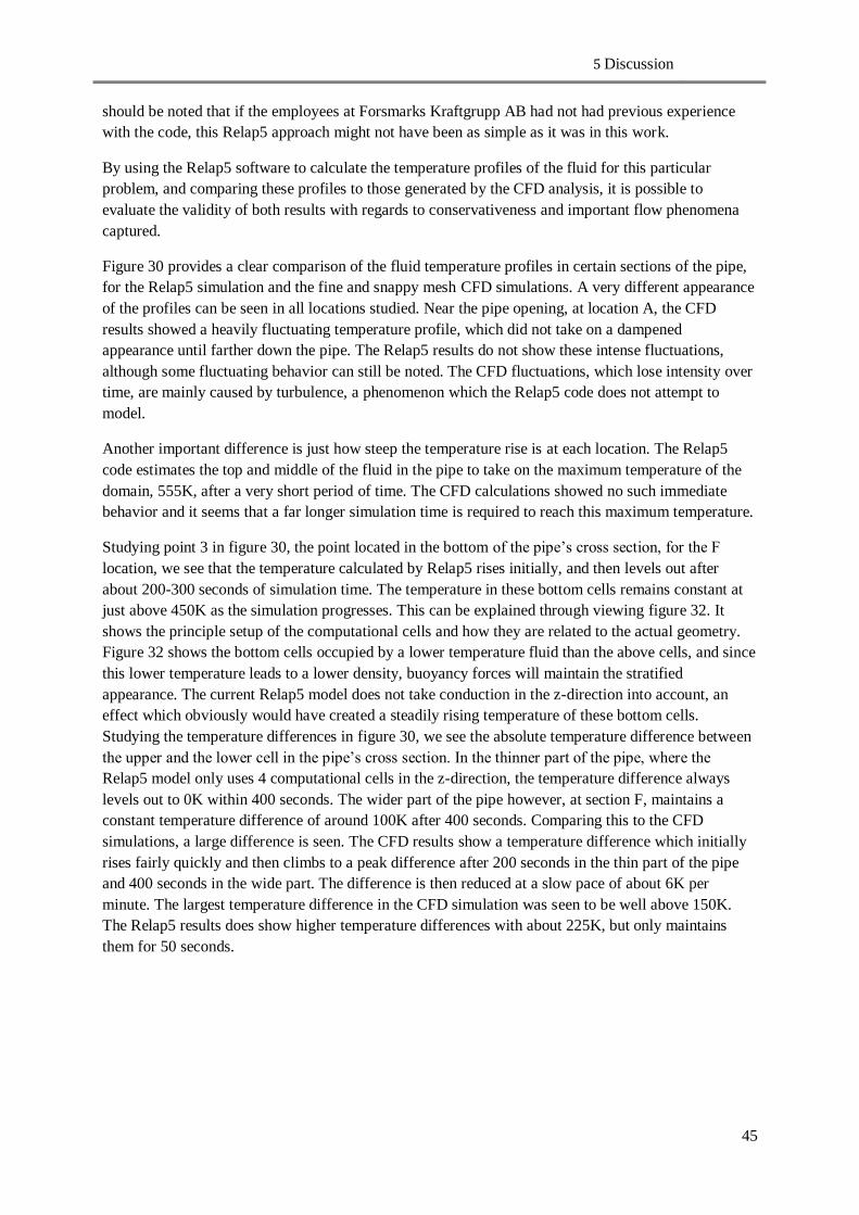
5 Discussion

45

should be noted that if the employees at Forsmarks Kraftgrupp AB had not had previous experience

with the code, this Relap5 approach might not have been as simple as it was in this work.

By using the Relap5 software to calculate the temperature profiles of the fluid for this particular

problem, and comparing these profiles to those generated by the CFD analysis, it is possible to

evaluate the validity of both results with regards to conservativeness and important flow phenomena

captured.

Figure 30 provides a clear comparison of the fluid temperature profiles in certain sections of the pipe,

for the Relap5 simulation and the fine and snappy mesh CFD simulations. A very different appearance

of the profiles can be seen in all locations studied. Near the pipe opening, at location A, the CFD

results showed a heavily fluctuating temperature profile, which did not take on a dampened

appearance until farther down the pipe. The Relap5 results do not show these intense fluctuations,

although some fluctuating behavior can still be noted. The CFD fluctuations, which lose intensity over

time, are mainly caused by turbulence, a phenomenon which the Relap5 code does not attempt to

model.

Another important difference is just how steep the temperature rise is at each location. The Relap5

code estimates the top and middle of the fluid in the pipe to take on the maximum temperature of the

domain, 555K, after a very short period of time. The CFD calculations showed no such immediate

behavior and it seems that a far longer simulation time is required to reach this maximum temperature.

Studying point 3 in figure 30, the point located in the bottom of the pipe’s cross section, for the F

location, we see that the temperature calculated by Relap5 rises initially, and then levels out after

about 200-300 seconds of simulation time. The temperature in these bottom cells remains constant at

just above 450K as the simulation progresses. This can be explained through viewing figure 32. It

shows the principle setup of the computational cells and how they are related to the actual geometry.

Figure 32 shows the bottom cells occupied by a lower temperature fluid than the above cells, and since

this lower temperature leads to a lower density, buoyancy forces will maintain the stratified

appearance. The current Relap5 model does not take conduction in the z-direction into account, an

effect which obviously would have created a steadily rising temperature of these bottom cells.

Studying the temperature differences in figure 30, we see the absolute temperature difference between

the upper and the lower cell in the pipe’s cross section. In the thinner part of the pipe, where the

Relap5 model only uses 4 computational cells in the z-direction, the temperature difference always

levels out to 0K within 400 seconds. The wider part of the pipe however, at section F, maintains a

constant temperature difference of around 100K after 400 seconds. Comparing this to the CFD

simulations, a large difference is seen. The CFD results show a temperature difference which initially

rises fairly quickly and then climbs to a peak difference after 200 seconds in the thin part of the pipe

and 400 seconds in the wide part. The difference is then reduced at a slow pace of about 6K per

minute. The largest temperature difference in the CFD simulation was seen to be well above 150K.

The Relap5 results does show higher temperature differences with about 225K, but only maintains

them for 50 seconds.

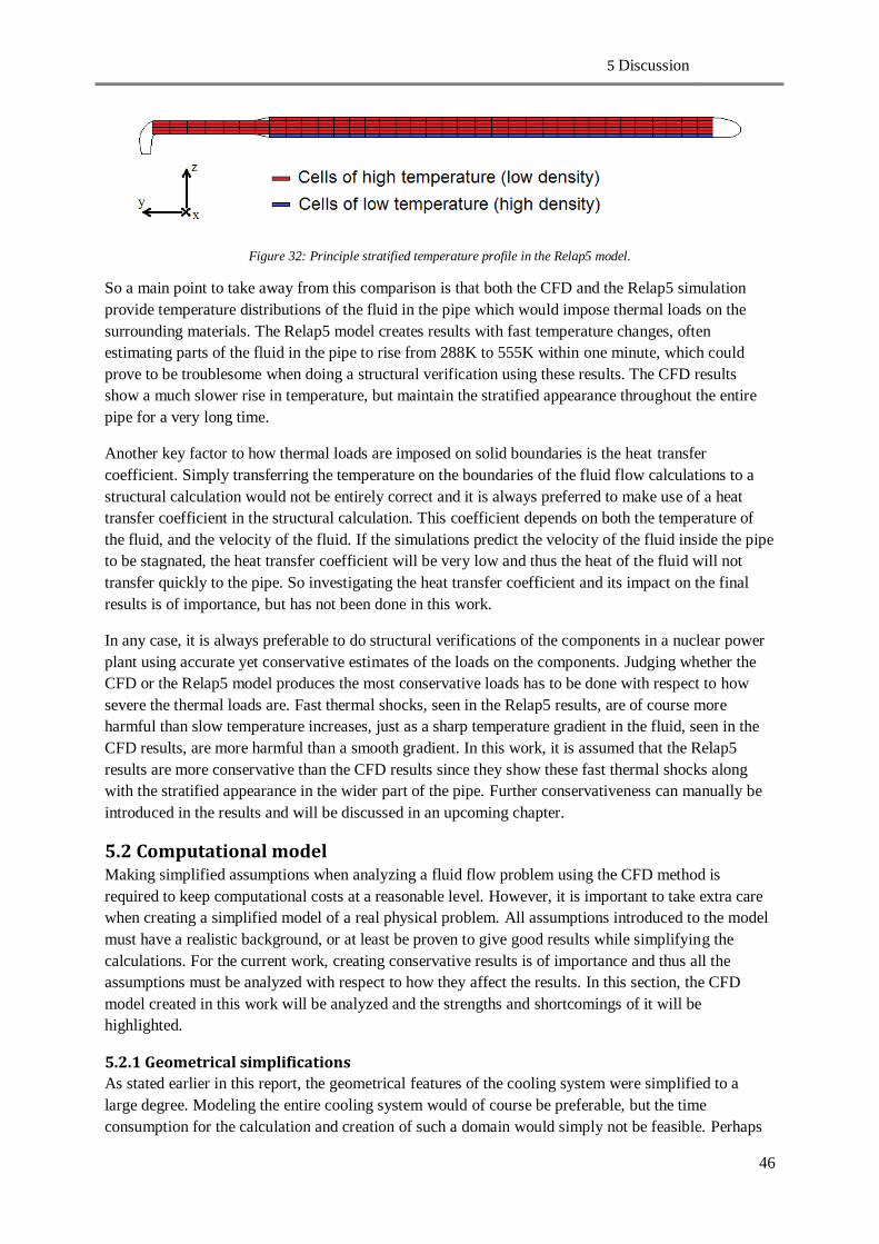
5 Discussion

46

Figure 32: Principle stratified temperature profile in the Relap5 model.

So a main point to take away from this comparison is that both the CFD and the Relap5 simulation

provide temperature distributions of the fluid in the pipe which would impose thermal loads on the

surrounding materials. The Relap5 model creates results with fast temperature changes, often

estimating parts of the fluid in the pipe to rise from 288K to 555K within one minute, which could

prove to be troublesome when doing a structural verification using these results. The CFD results

show a much slower rise in temperature, but maintain the stratified appearance throughout the entire

pipe for a very long time.

Another key factor to how thermal loads are imposed on solid boundaries is the heat transfer

coefficient. Simply transferring the temperature on the boundaries of the fluid flow calculations to a

structural calculation would not be entirely correct and it is always preferred to make use of a heat

transfer coefficient in the structural calculation. This coefficient depends on both the temperature of

the fluid, and the velocity of the fluid. If the simulations predict the velocity of the fluid inside the pipe

to be stagnated, the heat transfer coefficient will be very low and thus the heat of the fluid will not

transfer quickly to the pipe. So investigating the heat transfer coefficient and its impact on the final

results is of importance, but has not been done in this work.

In any case, it is always preferable to do structural verifications of the components in a nuclear power

plant using accurate yet conservative estimates of the loads on the components. Judging whether the

CFD or the Relap5 model produces the most conservative loads has to be done with respect to how

severe the thermal loads are. Fast thermal shocks, seen in the Relap5 results, are of course more

harmful than slow temperature increases, just as a sharp temperature gradient in the fluid, seen in the

CFD results, are more harmful than a smooth gradient. In this work, it is assumed that the Relap5

results are more conservative than the CFD results since they show these fast thermal shocks along

with the stratified appearance in the wider part of the pipe. Further conservativeness can manually be

introduced in the results and will be discussed in an upcoming chapter.

5.2 Computational model Making simplified assumptions when analyzing a fluid flow problem using the CFD method is

required to keep computational costs at a reasonable level. However, it is important to take extra care

when creating a simplified model of a real physical problem. All assumptions introduced to the model

must have a realistic background, or at least be proven to give good results while simplifying the

calculations. For the current work, creating conservative results is of importance and thus all the

assumptions must be analyzed with respect to how they affect the results. In this section, the CFD

model created in this work will be analyzed and the strengths and shortcomings of it will be

highlighted.

5.2.1 Geometrical simplifications

As stated earlier in this report, the geometrical features of the cooling system were simplified to a

large degree. Modeling the entire cooling system would of course be preferable, but the time

consumption for the calculation and creation of such a domain would simply not be feasible. Perhaps

5 Discussion

47

the geometrical simplification which affects the results the most would be to not include the elaborate

suspension system for the pipe insert. The suspension is positioned as close to 3D from the mouth of

the pipe, and continues all the way to the vessel wall. It should be noted that this simplification is

mainly made to decrease the complexity of the meshing stage. Manually creating a computational grid

around this complicated geometrical feature is time consuming and it will increase the difficulty of

maintaining a good mesh quality throughout the domain. Instead, the domain boundary was placed 3D

from the mouth of the pipe, completely leaving out this complicated region of the geometry. It would

definitely be of interest to investigate how much of an impact the suspension system has on the flow

field, and how it will affect the flow of warm water into the pipe insert as this could lead to

conclusions on just how simplified the geometry of a buoyancy driven flow problem can be. Such an

investigation will be left as future work.

The real pipe insert is surrounded by a thermal insulation, which was not included in the

computational domain. Accurately capturing the flow field in such geometries, which are similar to

those of plate heat exchangers, is difficult and resolving the flow dynamics within them would require

a sufficiently fine mesh which would further increase the computational cost. Including the insulation

in the model would introduce another unknown into the problem and just judging whether or not the

modelling of it is correct would require far more work than what is reasonable for this project. Other

solutions to this problem, such as introducing a porous media in place of the thermal insulation, will

be discussed in the future work segment.

It should be pointed out that by ignoring the effect of the thermal insulation, more thermal energy will

be kept inside the pipe, and transported out of the reactor pressure vessel. Therefore, this can be seen

as a simplification made with conservativeness in mind, as the components will be exposed to a larger

heat gradient than they would if the insulation was there.

The distance from the upper boundary of the downcomer region to the pipe insert needed to be long

enough for the flow in the downcomer to develop and become fairly steady. Placing the inlet to the

downcomer region too close to the pipe could create a situation where the flow behaves unrealistically,

whereas too far away would simply be a waste of computing time.

Extending the domain sufficiently below the mouth of the pipe is also an issue to be concerned with.

When simulating the pump driven flow, a jet forms below the mouth of the pipe (see figure 21). The

length of this jet is difficult to estimate without initial simulation tests, but it is almost certain that it

will not be a coherent jet very far below the mouth of the pipe, but rather break up and disperse its

momentum to the fluid around it. It was decided that the coherent jet should be captured in the

domain, as well as some part of the region below the jet where it has broken up. It would be preferable

to extend the domain downwards far enough from the jet so that the flow field regains a stable profile,

although this would also increase the computational time significantly. The flow can be seen to be

very chaotic in appearance even near the outlet of the domain, which could cause some stability issues.

Versteeg & Malalasekera[3] notes that sizeable errors may occur if an outlet boundary (using a zero

gradient velocity condition) is placed in a region where the flow is not fully developed. However,

since the pump driven flow and the flow field in the lower regions of the downcomer are not of

particular interest in this work, having a badly positioned outlet is not a major concern. Furthermore,

stability issues caused by backflow occurring at the outlet were not found to be an issue.

5.2.2 Heat transfer simplifications

The effects radiation has on any fluid flow problem depend on a number of factors such as the

temperature ranges involved in the domain and the magnitude of the other modes of heat transfer:

5 Discussion

48

convection and conduction. If, for example, conduction is negligible and the flow velocities in the

problem are small, meaning heat transfer by convection is small, the radiative heat flux can have a

considerable impact on the total heat fluxes in the domain. However, taking radiation effects into

account when analysing a problem using the CFD method will increase the complexity of the model

and bring further uncertainties into the solution. A separate radiation model must be introduced and

several exist[3], although all require special attention in order to give accurate results. A modification

of the governing equations for the fluid is needed if the fluid itself can absorb and emit radiative

fluxes.

Focusing on the present case, the radiation heat transfer phenomenon could be of major importance

when studying the temperature profiles in the cooling pipe. As seen in figure 22, a stratified field of

warm and cold water occupies the pipe region, and it is reasonable to think that the surrounding pipe

would also have this distinct temperature gradient. The difference between the highest temperature in

the warm layer and the lowest in the cold layer were found to be almost 200K in certain regions of the

pipe. Water is an efficient absorber and emitter of radiative heat fluxes so radiation immediately from

the upper part of the pipe to the lower part would be inhibited, but the temperature of the fluid would

surely be affected. Heat transfer from radiation could result in a smoother temperature gradient in the

cross section of the pipe, although this is only speculation.

A perhaps even greater simplification is to not model heat flux from the fluid to the solid region in the

domain. That is, to take into account the pipe structure being heated or cooled, and also how the

temperature varies through this solid. There are implemented solvers in OpenFOAM 2.3.x which can

couple a fluid and solid domain and the heat transfer between the two. The solid region would

obviously have to be given correctly chosen material properties, as well as a separate computational

mesh adjacent to the fluid region. Using the coupled fluid-solid model approach to capture the

temperature in the structure would however require the geometry of the solids to be accurate. Due to

several geometrical simplifications around the pipe insert, primarily the omitting of the thermal

insulation surrounding the pipe, the conjugate heat transfer would not be accurate here. An alternative

approach could be to consider the effect of heat conduction through the solids only in certain areas,

such as the pipe outside of the reactor pressure vessel, where no insulation is fitted. The geometry in

this region is fairly accurate (apart from omitting the suspension system for the pipe structure) and so

the conjugate heat transfer may produce accurate results. It should be stressed that the inclusion of the

solid region in the model would be done purely to capture the effect it has on the flow field, and not to

do a structural analysis.

5.2.3 Boundary conditions

On the topic of choosing the correct boundary conditions, one must base their choice on experience

and common sense. Whether or not the condition would be a good representation of the real boundary

is not always a trivial question to answer, especially when a boundary has been created in the

computational model which is not present in the problem being modeled. In the current work, the four

parallel sides of the downcomer region were given symmetry boundary conditions. Considering the

placement of the two boundaries situated closest to the internal surface of the reactor pressure vessel

and the reactor core shroud respectively (see figure 33), it is easy to see that a no-slip wall boundary

condition may be better suited. The perhaps best solution, without having to decide which boundary

condition is the most accurate, would be to extend the domain all the way to the vessel and core

shroud walls as depicted in figure 33. This was decided against as it was speculated early on that the

computational cost of the simulations would very high, even with the smaller domain. The same

reasoning was used for not extending the other two symmetry boundaries.

5 Discussion

49

Figure 33: Larger domain boundaries.

The symmetry condition implies there is no flow across the boundary. Considering the buoyancy

driven flow in the simulation, the flow in the downcomer could be seen as fairly stable, at least near

the sides of the computational domain. The bluff body of the pipe insert would of course interrupt the

stable flow and perhaps cause the flow to be directed out through the sides of the domain, and the

symmetry boundary conditions would then be improper. The symmetry boundary imposes an

unphysical constraint on the turbulent structures, even in cases where geometry and the time-averaged

variables are symmetric with respect to the boundary. Periodic boundary conditions would be better

suited as they do not impose any constraints on the resolved turbulence, although these conditions

imply whatever quantities exits one of the boundaries, must enter the other boundary, which of course

is not entirely correct.

A brief investigation was made regarding the boundary condition on the downcomer side closest to the

pressure vessel side (purple in figure 17). In order to further motivate the use of the symmetry

boundary condition, the boundary condition was changed to the perhaps more intuitively chosen no-

slip wall boundary condition as noted in table 5 in the appendix. The purpose of this investigation was

to see if the simulation results depend heavily on which condition is specified on this specific

boundary.

Shown in figure 31 are the temperature profiles of said investigation, along with profiles from a

reference simulation in which the only difference was the boundary condition. We see a very good

agreement between the two cases; only small discrepancies can be noted. The main difference to note

is how the initial temperature rise is slightly higher for the reference case (see location F), although

this difference is only of about 10K, and remains the same throughout the simulations. The time it

takes for the warm water to reach the back of the pipe region (location F in figure 28) is roughly the

same for both cases. So whether the specified boundary condition is a symmetry condition or a no-slip

wall condition does not seem to have a significant impact on the results in any way.

Using wall functions to model the flow field close to walls is an approach used when the mesh is too

coarse to properly resolve the boundary layer. However, wall functions can only model the flow

accurately when used within their operating limits. Having a too coarse or too fine boundary mesh can

cause the functions to perform poorly and it is difficult to create a proper boundary mesh for a

complex geometry. Wall functions especially have troubles modeling a correct flow field when the

5 Discussion

50

flow is detached from solid boundaries and should simply not be used in those regions. Since the flow

in the domain studied in this work was not expected to behave similarly across all wall boundaries, no

wall functions were used. This would probably mean the boundaries would require a much finer mesh

to resolve the flow field properly.

Giving the inlet boundary a uniform steady velocity profile is also questionable, considering the

various components positioned above the pipe insert (see figure 4). The main feedwater system is not

sufficiently far away from the inlet boundary of the computational domain for the flow conditions to

be considered stable. Surely, a fluctuating profile would be present here, and it would also depend on

the current operating scenario of the power plant. Prescribing a stable velocity profile directed

downward on the downcomer inlet could potentially flaw the results. However, a somewhat correct

inlet velocity profile is virtually impossible to obtain without doing costly analyses on the flow field

above the domain, which is obviously out of the scope of this thesis. A simpler solution would be to

apply a mildly fluctuating velocity profile on the inlets to represent the instabilities. However, the

velocity profile discrepancies are not expected to have a large impact on the results.

5.2.4 Initial conditions

The arguably most interesting flow condition in this work is the buoyancy driven flow, as opposed to

the pump driven flow. Since the analyses of cooling systems such as this one are mainly geared

towards studying the temperature field in the fluid, a flow scenario such as the pump driven flow is not

of much interest. Since the fluid velocity inside the pipe is very high during the pump driven flow

(above 2m/s in the slowest region), the temperature within the pipe is predicted to be stable. The

temperature around the pipe insert inside of the reactor pressure vessel can also be assumed to remain

stable during the pump driven flow. The mixing process of water with varying density in the

downcomer and other parts of the nuclear reactor is an interesting topic to study and have analyzed

been in several works ([21], [22],[23]), although is not the focus of this work.

Considering this, the pump driven flow stage can be seen as the creating of initial conditions for the

buoyancy driven flow. Turbulent structures form in the initialization process, both in the pipe region

and in the downcomer region. A long initialization process is preferable as this will mature the

turbulent structures and make the flow field statistically steady state. It is possible to analyze

fluctuating quantities such as velocities and temperature to make sure the flow field has reached a

sufficiently developed state, although this approach was not used in the current work. Instead, it was

assumed that three flow-throughs (6 seconds of simulation time) of a particle from the inlet of the pipe

to the outlet of the downcomer would be sufficient for all relevant turbulent structures to form in the

domain. The temperature distribution in the downcomer region showed no significant change after six

seconds had passed. The linear transition from the pump driven stage to the buoyancy driven stage,

where the inlet velocity is reduced to 0m/s over the course of one second, is also a factor affecting the

initial conditions. The real scenario of halting the flow of cooling water would with all certainty be

very different than the scenario simulated. A check valve installed on the cooling system is the

component which stops the cooling procedure, and the characteristics of this component, such as the

shutting speed, are not easy to approximate. How this flaw in the simulation model impacts the overall

results is hard to tell, but is probably not noteworthy especially far into the buoyancy driven flow.

There are ways to approximate how the velocity changes as the check valve shuts by using simulation

tools such as the Relap5 software, but the linear transition of the inlet velocity was seen as good

enough for simplistic reasons.

5 Discussion

51

5.2.5 Choice of turbulence model and numerical solver properties

Modeling turbulence can be done in numerous ways, and the choice of turbulence model is often a

question of computational costs. Generally, turbulence models which numerically resolve parts of the

turbulent spectrum are more expensive than those which model the entire spectrum. Using the

Reynolds Averaged Navier-Stokes (RANS) equations implies modelling the entire turbulent spectrum,

often by using two-equation models to simulate the turbulent behavior. Applying these equations to

the current problem would require the use of the unsteady RANS (URANS) method of modelling

turbulence, since the problem at hand is inherently transient. Scheurer et al. [22] performed CFD

calculations on a flow problem involving coolant injection into a pressurized water tank, and

compared these with experimental results on a similar domain. They used both an URANS approach

of modelling turbulence, as well as the more costly ω-based Reynolds Stress Model (RSM) approach.

They noted that a modification of the URANS turbulence models is needed when simulating fluid

flow problems which have a stratified temperature field. Extra turbulence production and destruction

terms due to buoyancy effects are needed in the model to achieve accurate results. Furthermore,

Scheurer et al. found that the URANS models could not accurately predict temperature oscillations in

the domain, a phenomenon of great importance in the study of nuclear reactor safety. It is these

oscillations which can cause thermal fatigue of components, and although this particular phenomenon

was not investigated in this work, it is important to take note of their existence and how to capture

them accurately.

Scheurer et al. noted that the RSM model provide good results for their particular flow problem, which

bares many similarities to the current work such as having large density gradients within the fluid, and

a stratified appearance of the temperature field in certain regions of the domain. The work of Höhne &

Kliem [21] also carries these similarities, in which the mixing properties of two fluids with different

densities inside a reactor pressure vessel were investigated. This investigation was carried out using

experiments and compared with CFD results, in which an ω-based RSM was used. The CFD

simulations were found to provide good qualitative results, showing a flow field similar to the

experimental results. However, the authors noted the results lacked accuracy in some local points in

the domain and their recommendation was to use a more advanced turbulence model, such as the

hybrid RANS/LES model DES (Detached Eddy Simulation).

The application of the LES turbulence modelling technique in the current work can be motivated from

several sources, including the above. Mahaffy et al. [24] states that LES is an approach suitable for

flows involving the buoyancy phenomenon, as buoyancy effects take place at large scales and LES,

provided a good computational mesh is used, manages to resolve all large turbulent scales in the flow

field. Ignoring the buoyancy effects stemming from the smaller scales, no additional terms needs to be

included in the turbulence model. LES can be successfully used for moderate Reynolds number flows

even in complex geometries, according to Mahaffy et al., if the CPU resources are sufficient.

In general, it was difficult to find works which dealt with similar flow dynamics as the ones seen in

this project, and also utilized LES turbulence modeling. It was therefore interesting to get some

knowledge on what kind of results could be expected from using LES. Fluctuating temperatures were

seen in all simulations and is, as previously stated, of great importance in thermal fatigue calculations.

Even though Scheurer et al. [22] stated that these fluctuations were not properly captured using the

URANS models, it would still be interesting to compare URANS results with LES results.

Unfortunately, setting up a proper URANS simulation would be too time consuming for this project.

Some previous knowledge of using LES in OpenFOAM exists at Forsmarks Kraftgrupp AB, but the

company is of course always interested in increasing their know-how about the topic.

5 Discussion

52

The LES SGS model used in this work was chosen simply because it was the best suited model

amongst those available for the transient compressible solver buoyantPimpleFoam. A dynamic SGS

model is available, which uses two filtering operations to adapt the model to best fit the local flow

field rather than behaving the same throughout the entire domain. However, initial simulations run

with this model proved to give faulty results such as a negative SGS kinematic viscosity, implying

there is something wrong with the implementation or application of the model. This is unfortunate, as

the dynamic approach of modelling the SGS viscosities could potentially give different predictions of

the flow field and it would then be interesting to compare these results to the results from the SGS

model used here.

Further comparisons which would be interesting are the choice of solver application. The

buoyantPimpleFoam solver was the clear choice for this project, although a possible alternative would

be to use another implemented solver application, called buoyantBoussinesqPimpleFoam which

utilizes the Boussinesq approximation. This was decided against due to the large density differences in

the fluid domain, and how the Boussinesq approximation is only valid for small density differences. It

would of course be possible to create a CFD solver designed for this particular case, but that is beyond

the scope of this thesis.

The iterative solution procedure used in all simulations was PISO, although a brief investigation with

the PIMPLE procedure was made. The PIMPLE method forces the solution to converge below set

convergence levels by repeating the PISO loop several times, rather than just assuming a good

convergence is met, as what is done in the PISO method when the loop is only done once. The

PIMPLE method can then be seen as a way of creating tougher convergence criterions for the solution.

Figure 31 displays the results of the investigation. Although the PIMPLE algorithm was only used for

just over 100 seconds of the buoyancy driven stage in the simulation, the results are extensive enough

to be compared with those of the PISO algorithm. A very good agreement is seen in both graphs

presented, and it can be concluded that the PISO algorithm manages to converge the solution to a

sufficient level.

5.2.6 Ensuring conservativeness in the results

From a perspective concerning if the simplifications of the flow calculation will make the results more

or less conservative, it is hard to make a trustworthy prediction. Geometrical changes such as omitting

the lifting eye and the suspension system of the pipe insert can be considered minor and will probably

have little effect on the general results. It may be possible to create an even further simplified domain

and still achieve the desired results, namely the stratified temperature field and the slow temperature

increase of the fluid within the pipe region. If these two phenomena are seen in the results, one can be

certain that the geometry has not been overly simplified.

It is also difficult to make a good prediction of how changing the heat transfer setup of the problem

would affect the results. It is assumed that including radiation and conjugate heat transfer methods in

the calculations would only have a small impact on the final results. Choices of boundary conditions,

initial conditions and turbulence model were made strictly to be as realistic as possible, while still

being economical. In other words, conservativeness was not the driving force behind how these

choices were made. Therefore, since it is difficult to judge just how conservative the final results are, it

is often preferable to modify the final results to make sure they are conservative. For instance, the

stratified temperature gradient in the pipe region, during the buoyancy driven flow, can be split into

sections of constant temperature as shown in figure 34.

5 Discussion

53

Figure 34: CFD results vs. a more conservative temperature distribution.

This sectioned temperature distribution would put larger stresses on the surrounding material and

therefore make the results more conservative. Similar approaches can be taken for the transient

temperature profiles, as shown in figure 35.

Figure 35: CFD results vs. more conservative temperature profiles.

By having the temperature of the fluid rise in large increments rather than having a smoother profile,

the material surrounding the fluid will be put through a much tougher operating scenario, making the

structural calculations more conservative.

These are just two examples of how results from a fluid flow calculation can be modified to ensure

conservativeness for future structural investigations. The framework for making these modifications

will not be established in this work, but rather left as an option for future projects.

1 Fel! Ogiltigt resultat för tabell.

54

6 Conclusions A robust CFD model of the cooling system has been created using the OpenFOAM 2.3.x software and

simulations of a cooling scenario have been performed. The computational domain was simplified and

it was speculated that the simplifications did not have a significant impact on the results, meaning

detailed geometrical features are not necessary to obtain good results in this particular case.

Four computational meshes were created for the domain, and ranged in size from 0,14M cells to 3,2M

cells. One of the meshes was generated using the OpenFOAM 2.3.x utility snappyHexMesh, which

proved to be far less time consuming than creating a mesh in the ANSA software. The time

consumption for the simulations with each mesh also differed greatly, with the coarse and the snappy

mesh being far more economical than the medium and the fine mesh. Furthermore, it was found that

all meshes produced roughly the same results with only minor differences, pointing towards the case

not being very mesh sensitive.

A main issue is to make sure the results are conservative and, for example, do not underestimate the

intensity of thermal shocks or the sharpness of temperature gradients within the fluid. The calculation

results can be modified in the post-processing stage to become more conservative for use in future

structural calculations, although this has not been done in the present work.

When comparing the CFD results to those of a simpler 1D fluid flow analysis tool, Relap5, it was

found that the CFD tool could capture more interesting, and possibly more realistic, flow phenomena.

Although using the CFD method for analysing these types of problems is far more expensive than the

1D approach, the difference in accuracy may be of great importance. This is especially true in cases

where the 1D code is unable to predict large temperature gradients or fast thermal shocks. However, in

this particular problem it was concluded that the Relap5 software managed to capture the temperature

field well and it was assumed that it gave a conservative estimate of the transient temperature profiles

of the fluid and could therefore be used successfully in similar analyses. A different way to look upon

this is if a Relap5 analysis produces temperature profiles which are too conservative, making a

structural verification impossible to make, the CFD approach can be applied to the problem and

possibly give less conservative results. It should be noted that the heat transfer coefficient should also

be studied to make a definite decision on how the Relap5 results differ from the CFD results.

The general approach used in this work for investigating the CFD method for these types of flow

problems can be seen as successful. It eventually gave a broad scope of the strengths and weaknesses

of the method as well as the LES turbulence modelling approach. It also provided insight on how time

can be saved in the meshing stage simply by considering different software. The evaluation of the

CFD results would be stronger if there were experimental results of the case available in addition to

the Relap5 results. A more solid investigation would perhaps be to analyse a flow scenario which

already has an experimental basis. Overall, a lot of knowledge has been found regarding how to

simulate buoyancy driven flow using the CFD and LES methods.

6.1 Future work From a perspective of improving the simulations’ accuracy and credibility, several changes can be

made. Most of the changes regard the geometrical simplifications made in the current work. A more

complex geometry was avoided in order to simplify the ANSA meshing process. However, through

studying the snappyHexMesh utility, it was found that a complex geometry can be dealt with

automatically, with only minor inputs from the user. It would then be of interest to create a


55

computational domain including the suspension system (see figure 2) and other geometrical features,

and mesh it using the snappyHexMesh utility. In general, the functioning of the snappyHexMesh utility

should be studied further as it could reduce the time cost of any CFD analysis while still providing a

computational mesh of good quality.

With regards to how these types of problems should be dealt with in the future, it would also be

interesting to simplify the geometry further to investigate how sensitive the results are to the

geometrical features, such as the lifting eye on the pipe insert. If it can be found that simple geometries

represent the cases well, a large amount of time can be saved.

Future work also includes creating a framework for how the CFD results should be transferred to a

structural calculation. If conservativeness can be ensured in the CFD results, it would be preferable to

transfer the results directly to a structural calculation setup. However, if the CFD results cannot be

proven to be conservative, it would be recommended to divide the temperature field into sections

along the solid boundaries and the transient temperature data also needs to be modified. A script could

be created to do these tasks with as little user input as possible.


57

7 References

[1] "Forsmark 3 Tryck- och temperaturbelastningar i rörsystem inom RCPB", (2013), Forsmarks

Kraftgrupp AB, internal report

[2] "Reaktorsystem Forsmark 1 & 2 GK 3", (2013), Kärnkraftsäkerhet och Utbildning AB, internal

report

[3] "An Introduction to Computational Fluid Dynamics The Finite Volume Method", H. K. Versteeg

and W. Malalasekera, (2007), 2nd edition, Pearson Education Limited

[4] "CFD simulations of turbulent buoyant atmospheric flows over complex geometry: Solver

development in OpenFOAM", F. Flores, R. Garreaud, and R. C. Muñoz, (2013), Computers &

Fluids, volume 82 p. 1-13

[5] "Weather Prediction by Numerical Process", L. F. Richardson, (1922), Cambridge University

Press

[6] "Turbulent Flows", S. B. Pope, (2000), Cambridge University Press

[7] "Computational Methods for Fluid Dynamics", J. H. Ferziger and M. Perić, (1999), 2nd edition,

Springer-Verlag Berlin Heidelberg

[8] "Fundamentals of Heat and Mass Transfer", T. L. Bergman, A. S. Lavine, F. P. Incropera, and D.

P. DeWitt, (2007), 6th edition, John Wiley & Sons, Inc.

[9] "Heat Transfer", J. P. Holman, (1999), 8th edition, McGraw-Hill, Inc.

[10] "OpenFOAM User Guide", OpenFOAM Foundation, (2013), Version 2.2.2

[11] "Error Analysis and Estimation for the Finite Volume Method with Applications to Fluid Flows",

H. Jasak, (1996), Imperial College London (University of London)

[12] "International Association for the Properties of Water and Steam", http://www.iapws.org/,

Retrieved 2014-08-28

[13] "A CFD benchmarking exercise based on flow mixing in a T-junction", B. L. Smith, J. H.

Mahaffy, and K. Angele, (2013), Nuclear Engineering and Design, volume 264 p. 80-88

[14] "Solution of the Implicitly Discretised Fluid Flow Equations by Operator-Splitting", R. I. Issa,

(1985), Journal of Computational Physics, volume 62 p. 40-65

[15] "A calculation procedure for heat, mass and momentum transfer in three-dimensional parabolic

flows", S. V. Patankar and D. B. Spalding, (1972), International Journal of Heat and Mass

Transfer, volume 15 issue 10 p. 1787–1806


58

[16] "MODELING OF COMPRESSIBLE FLUID PROBLEMS WITH OPENFOAM USING DYNAMIC

MESH TECHNOLOGY", H. J. Aguerrea, S. M. Damiána, J. M. Gimeneza, and N. M. Nigro,

(2013), Mecánica Computacional, volume 32 p. 995-1011

[17] "RELAP5/MOD3 CODE MANUAL VOLUME V: USER'S GUIDELINES", C. D. Fletcher and R.

R. Schultz, (2001), Idaho National Engineering Laboratory and Lockheed Idaho Technologies

Company

[18] "ParaView", http://www.paraview.org, Retrieved 2014-08-28

[19] "Large Eddy Simulations: how to evaluate resolution", Lars Davidson, (2009), International

Journal of Heat and Fluid Flow, volume 30(5) p. 1016-1025, 2009

[20] "The Basic Equations for the Large Eddy Simulation of Turbulent Flows in Complex Geometry",

S. Ghosal and P. Moin, (1995), Journal of Computational Physics, volume 118 p. 24-37

[21] "Modeling of a buoyancy-driven flow experiment in pressurized water reactor using CFD-

methods", T. Höhne and S. Kliem, (2007), Nuclear Engineering and Technology, volume 29 p.

327-336

[22] "Evaluation of Computational Fluid Dynamics Methods for Reactor Safety Analysis", M.

Scheuerer et al., (2005), Condensed Final Summary Report,

http://cordis.europa.eu/documents/documentlibrary/72284491EN6.pdf, Retrieved 2014-08-22

[23] "Experimental studies and CFD calculations for buoyancy driven mixing phenomena", M. J. da

Silva, S. Thiele, T. Höhne, R. Vaibar, and U. Hampel, (2009), Nuclear Engineering and Design,

volume 240 p. 2185–2193

[24] "Best Practice Guidelines for the use of CFD in Nuclear Reactor Safety Applications", J. Mahaffy

et al., (2007), Nuclear Energy Agency

8 Appendix Presented in table 5 is the complete set of boundary conditions specified in the OpenFOAM software.

Table 5: Boundary conditions specified for the different properties in the OpenFOAM software. The “Pressure vessel side” boundary conditions were changed to match the “Walls of pipe” boundary conditions for a brief investigation described in chapter 3.3.2.

Boundary

Walls of pipe zeroGradient fixedValue

value: uniform 0

zeroGradient calculated

(from )

zeroGradient zeroGradient fixedValue

value: uniform (0 0 0)

Downcomer inlet zeroGradient fixedValue

value: uniform 2e-05


(from )

zeroGradient fixedValue

value: uniform 555

fixedValue

value: uniform (0 0 -0.468)

Downcomer outlet zeroGradient inletOutlet

inletValue: uniform 2e-05

value: uniform 0


(from )

fixedValue

value: uniform 0

inletOutlet

inletValue: uniform 555

value: uniform 555

zeroGradient

Pipe inlet zeroGradient fixedValue

value: uniform 2e-05


(from )

zeroGradient fixedValue

value: uniform 555

uniformFixedValue

uniformValue: table (0 (-1.8188903 1.9540089 0.4502707))

(6 (-1.8188903 1.9540089 0.4502707))

(7 (0 0 0))

Downcomer sides symmetry symmetry symmetry symmetry symmetry symmetry symmetry

Pressure vessel side symmetry symmetry symmetry symmetry symmetry symmetry symmetry

Presented in table 6 are the polynomials used to model the density , specific heat capacity , thermal conductivity and dynamic viscosity for the fluid.

Table 6: The polynomials used for modelling the temperature-varying fluid properties. Temperature is denoted T with unit [K].

Property Polynomial

CFD-analysis of buoyancy-driven flow inside a...

Documents

Transcript of CFD-analysis of buoyancy-driven flow inside a...